TRAJECTORY MODELING FOR SATELLITE IMAGE TRIANGULATION · TRAJECTORY MODELING FOR SATELLITE IMAGE...

TRAJECTORY MODELING FOR SATELLITE IMAGE TRIANGULATION

In-seong Jeong, James Bethel

Geomatics Engineering, School of Civil Engineering, Purdue University 550 Stadium Mall Drive, West Lafayette, IN, 47907 –

(ijeong, bethel)@purdue.edu

Commission I, WG I/5 KEY WORDS: Satellite photogrammetry, Sensor model, Mapping, support data, Trajectory model, Leave-one-out cross-validation ABSTRACT: The model components of satellite photogrammetry consist of a trajectory model, projection equations and parameter subset selection. The trajectory model is important because subsequent estimation is performed by making corrections or refinements to this initial path. However, satellite imagery products are provided with diverse formats of support data having different types, representations, frequencies and conventions. Among the three components of the sensor model, the construction of the position and attitude trajectory is closely linked with the availability and type of support data. In order to build a physical sensor model compatible with the metadata, a number of trajectory models have to be set up, and the influence of each trajectory model has to be analyzed. In order to investigate these issues in a practical way that is tied to real data, we show how trajectory models can be implemented based on support data from six satellite image types: Quickbird, Hyperion, SPOT-3, ASTER, PRISM, and EROS-A. Triangulation for each image is implemented to investigate the feasibility and suitability of the different trajectory models. Also, to evaluate the result, we used the leave-one-out cross-validation(LOOCV) method that enables effective use of a group of point observations, and provides independence to the check point selection and distribution. The results show the effectiveness of some of the simple models while indicating that careful use of dense ephemeris information is necessary. These results are based on having a number of high quality ground control points.

1. INTRODUCTION

Experience has shown that there is a natural linkage between the type of metadata supplied with a raw, basic, or level-0 (no geometric correction) satellite image and the physical sensor models used for triangulation of that imagery. As technology evolves, such metadata exhibits higher quality with higher frequency sampling rates. Nevertheless, different vendors and suppliers make different choices about what metadata to provide and about how to present it. Examples of such vendor choices include: reference coordinate system: earth fixed or inertial; data frequency: ranging from a few ephemeris points per image to hundreds; and parameterization of attitude data, presented as Euler angles or as quaternions. Such diversity presents a challenge to sensor model developers in requiring a detailed study of such metadata while constructing a compatible model. In an attempt to highlight these issues and to encourage a movement toward standardization of metadata presentation, we have done a study involving imagery from six medium to high resolution systems with the goal of evaluating different approaches for construction of the initial position and attitude trajectory and its refinement via the triangulation process.

2. MODEL COMPONENTS IN SATELLITE PHOTOGRAMMETRY

A rigorous, physical satellite sensor model can be thought of as having three components: A time-dependent reference or initial trajectory specification; a set of projection equations, usually over-parameterized; and an algorithm to select some subset of the trajectory and projection parameters for use in the actual estimation process. Note that when we speak of a trajectory it means a path through a six dimensional space including both position and attitude.

2.1 (Initial) Trajectory model

As Dowman and Michalis (2003) summarized, unlike frame camera geometry, due to the dynamic nature of pushbroom imaging geometry, each line has its own exterior orientation (EO) parameters. However those parameters cannot be individually considered in the model because information to recover explicitly the parameters of all scan lines is insufficient. Therefore we assume that the EO of adjacent lines is highly correlated and may be modeled by a low order function. This calls for a model to specify an initial trajectory of both position and attitude. This initial trajectory is important since subsequent estimation often entails making corrections or refinements to this initial path. The position and attitude along this trajectory should be a function of time, so that time-tagged line numbers can be unambiguously referenced to it. A trajectory model can be very complete and accurate with only small corrections required, or it can be very rough or simplistic, with significant departures built up during the estimation process. Such an initial trajectory can consist of, for example, Kepler elements or a sequence of discrete positions and attitudes. One may have to distinguish between the camera and the platform if they are not the same entity. Such a trajectory model describes the initial approximation of the time varying exterior orientation of the camera system. 2.2 Projection equations

A rigorous sensor model tries to reflect the geometry and physics of how the image is formed based on the well known collinearity condition. Unlike the frame camera model, the satellite sensor model should contain sufficient parameters to accommodate any permissible scanning motions. These scanning motions may be present in the initial trajectory or they may have to be built up during the estimation process. Also, it is

901

The International Archives of the Photogrammetry, Remote Sensing and Spatial Information Sciences. Vol. XXXVII. Part B1. Beijing 2008

a common strategy to model the small variations from the nominal trajectory as a low order polynomial with regard to scan line time. All of those factors are considered as known, unknown, or observed parameters in the projection equations. These equations treat the parameters of both interior orientation, IO, and EO. Note that this strategy of refining a given trajectory requires external information such as high quality ground control points. 2.3 Parameter subset selection

The photogrammetric projection equations are often over-parameterized and may therefore include highly correlated, or even dependent, parameters which may lead to singularity or solution instability. Including these dependent parameters should not be viewed as flawed model construction, rather it provides flexibility for the user to select an independent subset. This step is such an essential part of the modeling process that we formalize it as a separate process. The selection involves designating some variables as known and fixed, others as completely unknown, and still others as observed with a quantifiable uncertainty. Guidance for the selection process may come from the metadata characteristics, from the experience of the analyst, from the analysis of the dependency pattern of the refinement parameters, or from analysis of columns in the condition equation matrix. 2.3 Relation between the three model components

The three model elements just described are closely related when implementing photogrammetric triangulation. A good quality trajectory model ensures better performance of the projection equations. Often factors considered in the trajectory model become parameter elements in the projection equations. Also the trajectory model influences the parameter subset selection according to the quality of support data used to construct the trajectory. And clearly the parameterization of the projection equations limits the possible range of variables present in the subset model.

3. TWO APPROACHES FOR TRAJECTORY MODEL

As suggested by Ebner (1999) there are generally two approaches for the trajectory model. These are (1) the orientation point approach and (2) the orbital constraint approach. With the orientation point approach, at certain regular or irregular time intervals, position and attitude are determined (usually by auxiliary sensors on the satellite) and provided as orientation points, or ephemeris points. For any scan lines in between the observed points, a low order piecewise interpolation may be used to interpolate a position and attitude. Ebner points out that whereas this reduces the number of unknowns to a manageable number, it leaves much of the trajectory un-tethered to any physical model for the motion. The orbital constraint approach (Ohlhof et al, 1994) assumes that the imaging satellite moves along a smooth mathematical curve. All scan line exposure stations would therefore be constrained on this orbit path. For a short arc, the assumption of a “two-body” orbit may be used. This may be parameterized with six elements of a state vector or, equivalently, six Kepler elements. For more extended arcs additional force model parameters may be used. The basic idea of the orbital constraint was originally introduced in the early days of satellite photogrammetry (Case, 1961). This concept has been exploited in many published sensor models.

Regarding the attitude trajectory, older, strictly nadir looking cameras could derive attitude information from the position trajectory and its relation to the earth. For modern, agile, body-scanning instruments, such assumptions are clearly not valid. These instruments completely decouple the scanning motion from travel along the orbit path. In these cases an explicit sampling of the attitude trajectory, analogous to an orientation point, often coincident with it, is essential.

4. TYPES OF SUPPORT DATA

When deriving trajectory data for a particular satellite, it is important to check the available support data because its characteristics, e.g. quality and sampling rate, may influence the triangulation method (McGlone, 2004). Since there are multiple ways to specify a position and attitude trajectory, the trajectory model chosen for the triangulation is often closely related to the specification in the support data. For example, if ephemeris data is provided at a very low frequency it is usually not a good choice to select the orientation point approach. Conversely, if the data rate and quality are high, it may be convenient to adopt the orientation point approach rather than the orbit constraint approach. According to the decisions of the vendor, each sensor provides different types of support data having different formats, reference coordinate systems, date rates, representation, units, quality, statistical completeness, conventions and other characteristics. This also means that the three model components, described earlier for satellite photogrammetry, are sometimes slightly or greatly influenced by these factors, and have to be modified or adapted according to the support data type. Cooperation between the vendor and the photogrammetric engineer using the data is essential to ensure a complete and rigorous implementation of the sensor model for a specific sensor (de Venecia et al, 2006).

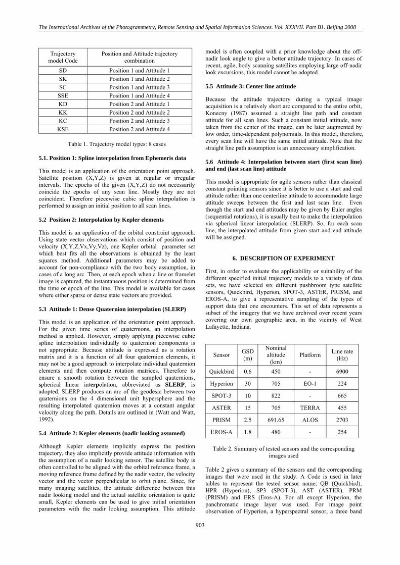
5. OVERVIEW OF TRAJECTORY MODELS

During the course of the triangulation or resection, an initial trajectory model will be refined (for short arcs) by low order polynomial corrections. This is illustrated in Figure 1 where the dotted lines show the initial exposure stations and directions of the optical axis as the sensor moves during scene acquisition. The solid lines show the refined location of exposure stations and refined attitudes.

Figure 1. Initial and refined trajectory illustration In Table 1., eight possibilities for the initial trajectory model are summarized, formed by all combinations of two position trajectory models and four attitude trajectory models. Details of each of these model are as follows.

902


Trajectory model Code

Position and Attitude trajectory combination

SD Position 1 and Attitude 1 SK Position 1 and Attitude 2 SC Position 1 and Attitude 3 SSE Position 1 and Attitude 4 KD Position 2 and Attitude 1 KK Position 2 and Attitude 2 KC Position 2 and Attitude 3

KSE Position 2 and Attitude 4

Table 1. Trajectory model types: 8 cases 5.1. Position 1: Spline interpolation from Ephemeris data

This model is an application of the orientation point approach. Satellite position (X,Y,Z) is given at regular or irregular intervals. The epochs of the given (X,Y,Z) do not necessarily coincide the epochs of any scan line. Mostly they are not coincident. Therefore piecewise cubic spline interpolation is performed to assign an initial position to all scan lines. 5.2 Position 2: Interpolation by Kepler elements

This model is an application of the orbital constraint approach. Using state vector observations which consist of position and velocity (X,Y,Z,Vx,Vy,Vz), one Kepler orbital parameter set which best fits all the observations is obtained by the least squares method. Additional parameters may be added to account for non-compliance with the two body assumption, in cases of a long arc. Then, at each epoch when a line or framelet image is captured, the instantaneous position is determined from the time or epoch of the line. This model is available for cases where either sparse or dense state vectors are provided. 5.3 Attitude 1: Dense Quaternion interpolation (SLERP)

This model is an application of the orientation point approach. For the given time series of quaternions, an interpolation method is applied. However, simply applying piecewise cubic spline interpolation individually to quaternion components is not appropriate. Because attitude is expressed as a rotation matrix and it is a function of all four quaternion elements, it may not be a good approach to interpolate individual quaternion elements and then compute rotation matrices. Therefore to ensure a smooth rotation between the sampled quaternions, spherical linear interpolation, abbreviated as SLERP, is adopted. SLERP produces an arc of the geodesic between two quaternions on the 4 dimensional unit hypersphere and the resulting interpolated quaternion moves at a constant angular velocity along the path. Details are outlined in (Watt and Watt, 1992). 5.4 Attitude 2: Kepler elements (nadir looking assumed)

Although Kepler elements implicitly express the position trajectory, they also implicitly provide attitude information with the assumption of a nadir looking sensor. The satellite body is often controlled to be aligned with the orbital reference frame, a moving reference frame defined by the nadir vector, the velocity vector and the vector perpendicular to orbit plane. Since, for many imaging satellites, the attitude difference between this nadir looking model and the actual satellite orientation is quite small, Kepler elements can be used to give initial orientation parameters with the nadir looking assumption. This attitude

model is often coupled with a prior knowledge about the off-nadir look angle to give a better attitude trajectory. In cases of recent, agile, body scanning satellites employing large off-nadir look excursions, this model cannot be adopted. 5.5 Attitude 3: Center line attitude

Because the attitude trajectory during a typical image acquisition is a relatively short arc compared to the entire orbit, Konecny (1987) assumed a straight line path and constant attitude for all scan lines. Such a constant initial attitude, now taken from the center of the image, can be later augmented by low order, time-dependent polynomials. In this model, therefore, every scan line will have the same initial attitude. Note that the straight line path assumption is an unnecessary simplification. 5.6 Attitude 4: Interpolation between start (first scan line) and end (last scan line) attitude

This model is appropriate for agile sensors rather than classical constant pointing sensors since it is better to use a start and end attitude rather than one centerline attitude to accommodate large attitude sweeps between the first and last scan line. Even though the start and end attitudes may be given by Euler angles (sequential rotations), it is usually best to make the interpolation via spherical linear interpolation (SLERP). So, for each scan line, the interpolated attitude from given start and end attitude will be assigned.

6. DESCRIPTION OF EXPERIMENT

First, in order to evaluate the applicability or suitability of the different specified initial trajectory models to a variety of data sets, we have selected six different pushbroom type satellite sensors, Quickbird, Hyperion, SPOT-3, ASTER, PRISM, and EROS-A, to give a representative sampling of the types of support data that one encounters. This set of data represents a subset of the imagery that we have archived over recent years covering our own geographic area, in the vicinity of West Lafayette, Indiana.

Table 2. Summary of tested sensors and the corresponding

images used Table 2 gives a summary of the sensors and the corresponding images that were used in the study. A Code is used in later tables to represent the tested sensor name; QB (Quickbird), HPR (Hyperion), SP3 (SPOT-3), AST (ASTER), PRM (PRISM) and ERS (Eros-A). For all except Hyperion, the panchromatic image layer was used. For image point observation of Hyperion, a hyperspectral sensor, a three band

Sensor GSD(m)

Nominal altitude

(km) Platform Line rate

(Hz)

Quickbird 0.6 450 - 6900

Hyperion 30 705 EO-1 224

SPOT-3 10 822 - 665

ASTER 15 705 TERRA 455

PRISM 2.5 691.65 ALOS 2703

EROS-A 1.8 480 - 254

903


RGB composite image was used assuming good inter-band coregistration. For ASTER, the VNIR (visible and near-infrared) 3B band was used for test. And for PRISM, CCD 4 (nadir looking image) was used for the test. Next, we have set up eight different initial trajectory models (two for position times four for attitude equals eight) to accommodate the diversity of support data that was given. We then implemented a collinearity-based rigorous sensor model for each sensor with each relevant initial trajectory model (not all trajectory models are possible with all sensors). The objectives of the experiment were to (a) investigate how triangulation results are influenced by the choice of trajectory model, (b) evaluate the applicability of different trajectory models to the specific support data provided with each image, and (c) based on the studies just described, determine a “best” trajectory model considering the image and support data characteristics.

support data interval

Sensor type # of data used time

(sec)

# of scan lines

Dense state vectors

(ECEF) 211 0.02 138

QB Dense

quaternion 211 0.02 138

Dense state vectors

(ECEF) 34 1

(average) 224 HPR

Dense quaternion 34 1

(average) 224

SP3 Sparse

state vectors (ECEF)

1 60 -

AST

Intermediate frequency

state vectors (ECEF)

15 0.8 360

Sparse state vectors

(ECEF) 9 1 2700

PRM Dense

quaternion 61 0.1 270

Sparse state vectors

(ECIN) 6 3.62 920

ERS Euler angles (orbital

reference frame)

2 (start-stop)

- -

Table 3. Used support data for each image in the study

A summary of the support for each image in the study is given in Table 3. The second column makes a distinction between reference coordinate systems: Earth Centered Earth Fixed, ECEF, versus Earth Centered Inertial, ECIN. For sensors having less than 300 lines between ephemeris point pairs, we declare them to be dense support data. The support data of Quickbird, Hyperion and the quaternions of PRISM

belong to this group. A line rate of more than 900 lines between ephemeris point pairs falls into the sparse data category. ASTER falls in between those two cases.

Trajectory model QB HPR SP3 AST PRM ERS

SD SK SC SSE KD KK KC

KSE

Table 4. Applicable trajectory model cases (shaded) according to the given support data

Table 4 shows the applicable trajectory model cases according to the given support data type. Quickbird and Hyperion provide dense support data and thus six trajectory models can be applied. Excluded is the attitude model using start and end Euler angles. For the other sensors, at least two models that utilize Kepler orbital elements are available to use. PRISM can use the dense quaternion interpolation model with 0.1 second rate quaternion data. EROS-A provides Euler angle information such via start and end attitude, and piecewise polynomial coefficients (although undocumented) to account for its non-synchronous scanning motion. For each model, a single image resection was performed using ground control points.

Sensor # of GCP Acquisition method

Quickbird 20 GPS surveying

Hyperion 45 Extracted from 1:24,000 scale map

SPOT-3 53 Extracted from 1:24,000 scale map

ASTER 21 Extracted from 1:24,000 scale map

PRISM 14 GPS surveying EROS-A 22 GPS surveying

Table 5. Number and source of GCP (Ground Control Point)

Table 5 shows the number and source of GCP used in the experiment. The extended, collinearity-based photogrammetric model has the form,

0

0 ( )L L

TA P N L A P N L

L L

x x X XXy y M M M Y Y M M M Y

Z Z Zfλ

− ⎡ Δ⎡ ⎤ ⎛ ⎞ ⎛ ⎞⎛ ⎞ ⎤⎢ ⎥⎜ ⎟ ⎜ ⎟⎜ ⎟⎢ ⎥− = − − Δ⎢ ⎥⎜ ⎟ ⎜ ⎟⎜ ⎟⎢ ⎥⎜ ⎟ ⎜ ⎟ ⎜ ⎟⎢ ⎥⎢ ⎥ Δ− ⎝ ⎠ ⎝ ⎠ ⎝ ⎠⎣ ⎦ ⎣ ⎦

(1)

where the variables are defined as follows, - (x,y) : Image coordinates within line or framelet - (X,Y,Z) : Ground coordinates with respect to ECEF

904


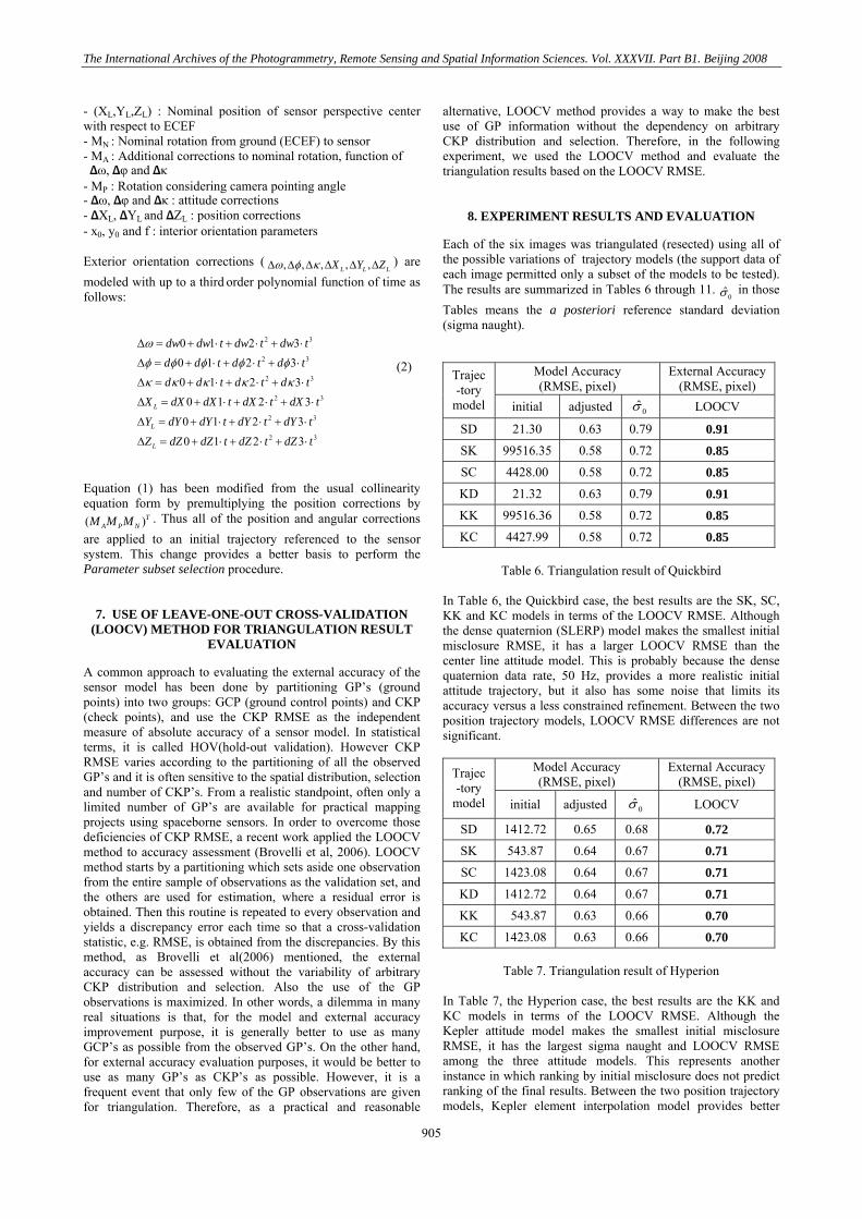
- (XL,YL,ZL) : Nominal position of sensor perspective center with respect to ECEF - MN : Nominal rotation from ground (ECEF) to sensor - MA : Additional corrections to nominal rotation, function of Δω, Δφ and Δκ - MP : Rotation considering camera pointing angle - Δω, Δφ and Δκ : attitude corrections - ΔXL, ΔYL and ΔZL : position corrections - x0, y0 and f : interior orientation parameters Exterior orientation corrections ( , , , , ,L L LX Y Zω φ κΔ Δ Δ Δ Δ Δ ) are modeled with up to a third order polynomial function of time as follows:

2 3

2 3

2 3

2 3

2 3

2 3

0 1 2 30 1 2 30 1 2 3

0 1 2 3

0 1 2 30 1 2 3

L

L

L

dw dw t dw t dw td d t d t d td d t d t d t

X dX dX t dX t dX t

Y dY dY t dY t dY t

Z dZ dZ t dZ t dZ t

ω

φ φ φ φ φκ κ κ κ κ

Δ = + ⋅ + ⋅ + ⋅

Δ = + ⋅ + ⋅ + ⋅

Δ = + ⋅ + ⋅ + ⋅

Δ = + ⋅ + ⋅ + ⋅

Δ = + ⋅ + ⋅ + ⋅

Δ = + ⋅ + ⋅ + ⋅

(2)

Equation (1) has been modified from the usual collinearity equation form by premultiplying the position corrections by

. Thus all of the position and angular corrections are applied to an initial trajectory referenced to the sensor system. This change provides a better basis to perform the Parameter subset selection procedure.

( TA P NM M M )

7. USE OF LEAVE-ONE-OUT CROSS-VALIDATION (LOOCV) METHOD FOR TRIANGULATION RESULT

EVALUATION

A common approach to evaluating the external accuracy of the sensor model has been done by partitioning GP’s (ground points) into two groups: GCP (ground control points) and CKP (check points), and use the CKP RMSE as the independent measure of absolute accuracy of a sensor model. In statistical terms, it is called HOV(hold-out validation). However CKP RMSE varies according to the partitioning of all the observed GP’s and it is often sensitive to the spatial distribution, selection and number of CKP’s. From a realistic standpoint, often only a limited number of GP’s are available for practical mapping projects using spaceborne sensors. In order to overcome those deficiencies of CKP RMSE, a recent work applied the LOOCV method to accuracy assessment (Brovelli et al, 2006). LOOCV method starts by a partitioning which sets aside one observation from the entire sample of observations as the validation set, and the others are used for estimation, where a residual error is obtained. Then this routine is repeated to every observation and yields a discrepancy error each time so that a cross-validation statistic, e.g. RMSE, is obtained from the discrepancies. By this method, as Brovelli et al(2006) mentioned, the external accuracy can be assessed without the variability of arbitrary CKP distribution and selection. Also the use of the GP observations is maximized. In other words, a dilemma in many real situations is that, for the model and external accuracy improvement purpose, it is generally better to use as many GCP’s as possible from the observed GP’s. On the other hand, for external accuracy evaluation purposes, it would be better to use as many GP’s as CKP’s as possible. However, it is a frequent event that only few of the GP observations are given for triangulation. Therefore, as a practical and reasonable

alternative, LOOCV method provides a way to make the best use of GP information without the dependency on arbitrary CKP distribution and selection. Therefore, in the following experiment, we used the LOOCV method and evaluate the triangulation results based on the LOOCV RMSE.

8. EXPERIMENT RESULTS AND EVALUATION

Each of the six images was triangulated (resected) using all of the possible variations of trajectory models (the support data of each image permitted only a subset of the models to be tested). The results are summarized in Tables 6 through 11.

0σ̂ in those Tables means the a posteriori reference standard deviation (sigma naught).

Model Accuracy (RMSE, pixel)

External Accuracy(RMSE, pixel)

Trajec-tory

model initial adjusted 0σ̂ LOOCV

SD 21.30 0.63 0.79 0.91 SK 99516.35 0.58 0.72 0.85 SC 4428.00 0.58 0.72 0.85 KD 21.32 0.63 0.79 0.91 KK 99516.36 0.58 0.72 0.85 KC 4427.99 0.58 0.72 0.85

Table 6. Triangulation result of Quickbird

In Table 6, the Quickbird case, the best results are the SK, SC, KK and KC models in terms of the LOOCV RMSE. Although the dense quaternion (SLERP) model makes the smallest initial misclosure RMSE, it has a larger LOOCV RMSE than the center line attitude model. This is probably because the dense quaternion data rate, 50 Hz, provides a more realistic initial attitude trajectory, but it also has some noise that limits its accuracy versus a less constrained refinement. Between the two position trajectory models, LOOCV RMSE differences are not significant.



Trajec-tory


SD 1412.72 0.65 0.68 0.72 SK 543.87 0.64 0.67 0.71 SC 1423.08 0.64 0.67 0.71

KD 1412.72 0.64 0.67 0.71 KK 543.87 0.63 0.66 0.70 KC 1423.08 0.63 0.66 0.70

Table 7. Triangulation result of Hyperion

In Table 7, the Hyperion case, the best results are the KK and KC models in terms of the LOOCV RMSE. Although the Kepler attitude model makes the smallest initial misclosure RMSE, it has the largest sigma naught and LOOCV RMSE among the three attitude models. This represents another instance in which ranking by initial misclosure does not predict ranking of the final results. Between the two position trajectory models, Kepler element interpolation model provides better

905


LOOCV RMSE than the spline interpolation model does, but their differences are not significant.



Trajec-tory


KK 47.71 0.69 0.74 0.78 KC 662.83 0.69 0.74 0.78

Table 8. Triangulation result of SPOT-3

In Table 8, the SPOT-3 case, the best results come from the KK and KC models in terms of the LOOCV RMSE.



Trajec-tory


KK 1759.43 0.51 0.60 0.73 KC 1764.18 0.51 0.60 0.73

Table 9. Triangulation result of ASTER

In Table 9, the ASTER case, the best results come from the KK and KC models in terms of the LOOCV RMSE.



Trajec-tory

model initial adjusted 0σ̂ initial

KD 143.24 0.85 1.01 1.22 KK 225.64 0.84 0.99 1.22 KC 407.89 0.84 0.99 1.23

Table 10. Triangulation result of PRISM

In Table 10, the PRISM case, the best results come from the KD and KK models in terms of the LOOCV RMSE of check points. In this case, initial misclosure RMSE of the KC model is the largest among other models, but the LOOCV RMSE is not significantly different.



Trajec-tory


KK 102606.11 1.13 1.39 1.99 KC 13534.88 1.17 1.45 2.05

KSE 2720.66 1.04 1.28 1.88

Table 11. Triangulation result of EROS-A In Table 11, the EROS-A case, the best result comes from the KSE model in terms of the LOOCV RMSE. The scan angle excursion in this case was larger than others. That is likely related to the improved performance when the start and end attitudes are specified. In case of the KK and KC models, though it may not fit to EROS-A, a body scanning agile sensor, the RMSE result looks reasonable. This is probably because the Kepler attitude model still provides initial angles within the

convergence range. This was an unexpected but interesting outcome.

9. CONCLUSIONS

The overall accuracy differences between the two position trajectory models are quite small. It is also expected that the RMSE difference may be smaller when denser orientation points are provided. That conclusion, of course, assumes that one has high quality control points, as in this study. If that were not the case, then the conclusions would be quite different. Despite the simplicity of the center line attitude model, the RMSE from that model is the best among others in the case of Quickbird, Hyperion, SPOT and ASTER. Therefore it appears that this simple model can be judged very effective. That the dense attitude information provides a better initial misclosure RMSE, but the final LOOCV RMSE result is not better, is probably due to the presence of a noise component in these observations. Therefore care has to be taken when using this dense attitude information. For sensors making large angle excursions during image acquisition without high frequency attitude sampling, such as Eros, it is desirable to know the start and end attitudes. The experiment shows that even this limited information about the attitude trajectory, only the two points, is sufficient to allow recovery of the full attitude excursion. A general conclusion from this work is a confirmation of our suspicion that standards and consistent presentation of support data are sorely needed for satellite images. Physical sensor modeling has powerful advantages, but they are diminished if the analyst must expend unproductive effort interpreting each vendor’s unique presentation of position and attitude support data. International societies and working groups together with government and industry representatives should cooperate in defining and enforcing such standards.

REFERENCES

Brovelli, M., Crespi, M., Fratarcangeli, F., Giannone, F. and Realini, E, 2006. Accuracy assessment of High Resolution Satellite Imagery by Leave-one-out method. Proceedings of the 7th International Symposium on Spatial Accuracy Assessment in Natural Resources and Environmental Sciences, 5–7 July 2006, Lisbon, Portugal, pp. 533-542. Case, J., 1961. The utilization of constraints in analytical photogrammetry. Photogrammetric Engineering and Remote Sensing, 25(5), pp. 766-788. de Venecia, K., Paderes, F. and Walker, S., 2006. Rigorous Sensor Modeling and Triangulation for OrbView-3. ASPRS 2006 annual conference, Reno Nevada. Dowman, I., and Michalis, P., 2003. Generic rigorous model for along track stereo satellite sensors, Proceedings of ISPRS Workshop 2003: High Resolution Mapping from Space, Hannover, Germany. Ebner, H., Kornus, W., Ohlhof, T. and Putz, E. 1999. Orientation of MOMS-02/D2 and MOMS-2/PPRIRODA imagery, ISPRS Journal of Photogrammetry & Remote Sensing, 54, pp. 332-341. Konecny, G., Lohmann, P., Engel, H. and Kruck, E., 1987. Evaluation of SPOT imagery on analytical photogrammetric

906


instruments. Photogrammetric Engineering and Remote Sensing, 53(9), pp. 1223-1230. McGlone, J., 2004. Manual of Photogrammetry. Fifth edition. American Society of Photogrammetry and Remote Sensing, Bethesda, MD., pp. 884-887. Ohlhof, T., Montenbruck, O. and Gill, E.,1994. A new approach for combined bundle block adjustment and orbit determination

basedonMars-94three-line scanner imagery and radio tracking data, International Archives of Photogrammetry and Remote Sensing, 30(3), pp. 630-639. Watt, A. and Watt, M., 1992. Advanced animation and rendering techniques: theory and practice. ACM Press, New York, NY, pp. 361-368.

907


908

TRAJECTORY MODELING FOR SATELLITE IMAGE TRIANGULATION · TRAJECTORY MODELING FOR SATELLITE IMAGE...

Documents

Transcript of TRAJECTORY MODELING FOR SATELLITE IMAGE TRIANGULATION · TRAJECTORY MODELING FOR SATELLITE IMAGE...