Trajectory Estimation of Bat Flight Using a Multi-View Camera System

Trajectory Estimation of Bat Flight Using a

Multi-View Camera System

Matt J. Bender∗ , Hunter G. McClelland † , Gerardo Bledt ‡ ,

Andrew Kurdila § , Tomonari Furukawa ¶ , and Rolf Mueller ‖

Virginia Tech, Blacksburg, VA, 24060, USA

The high maneuverability and stability of biological fliers has re-ignited research in flap-ping wing flight mechanics in the last 10 years. Research to date has studied the kinemat-ics, dynamics, and aerodynamics of bats to determine how they maneuver. This researchrequires motion capture studies of a specimen in flight to determine wing and body mo-tion. A key difficulty in using motion capture techniques is frequent point occlusion whichis caused by the highly articulated nature of bat wings during flight. In this paper wepresent extended and unscented Kalman filter algorithms that are derived for multi-viewmotion capture experiments with highly redundant camera configurations. Two experi-mental data sets are studied in this paper. The first contains bat ear motion capture dataobtained using two low-distortion cameras; this data is used to validate the Kalman filteralgorithms. The second set includes bat flight data which uses 5 high-distortion camerasthat are employed to estimate inertial trajectory reconstruction.

∗PhD Student, Mechanical Engineering, 144 Durham Hall, Blacksburg, VA 24060, AIAA Student Member†PhD Student, Mechanical Engineering, 144 Durham Hall, Blacksburg, VA 24060‡BS Student, Mechanical Engineering and Computer Science, 144 Durham Hall, Blacksburg, VA 24060§W. Martin Johnson Professor, Mechanical Engineering, 141 Durham Hall, Blacksburg, VA 24060¶Professor, Mechanical Engineering, 225 Goodwin Hall, Blacksburg, VA 24060‖Associate Professor, Mechanical Engineering, 312 ICTAS II, 1075 Life Science Circle, Blacksburg, VA 24060

Director, Taishen Professor, SDU-VT International Laboratory, Shandong University, Jinan, Shandong, China

1 of 13

American Institute of Aeronautics and Astronautics

Nomenclature

α = Flap Angle Measurement

A = State Transition Matrix

C = Coriolis Matrix

d = Distance

f = Frequency

h(·, ·) = Observation Function

h(·) = Measurement Model

Hc0 = Homogeneous Transform from Inertial Basis (0) to Camera Basis (c)

H = Jacobian of the Measurement Model

i = Point Index Variable

I = Identity Matrix

j = Camera Index Variable

K = Camera Calibration Matrix

λ = Z-coordinate of Feature Point in Camera Basis

m = Number of Cameras

M = Mass Matrix

n = Number of Points

Qk = Correction Covariance at time step k

φ = Pixel Coordinates of Feature Point

Π0 = Canonical Projection Matrix

Rk = Prediction Covariance at time step k

� = State Covariance Matrix

τ = Joint Torque Vector

θ = Joint Angle Vector

UT = Unscented Transform

v = Point Velocity

V = Potential Energy Function

v = Measurement Noise Vector

w = Process Noise Vector

x = Point in Inertial Coordinates

xk = State Vector [3n× 1] at time step k

Xk = Matrix of Sample Points

yk = Observation Vector [2nm× 1] at time step k

Yk = Measurement of Predicted Sample Points

I. Introduction

A number of investigators have studied the complexity of flapping flight in bats where experiments arebased on placing markers on bat wings and subsequently collecting video of various flight regimes.1,2

The video is used to reconstruct three dimensional trajectories of the fiducial markers in inertial space.3,4, 5

These trajectories are subsequently used to study the complexity of the highly articulated motion observedduring bat flight,6 and they are likewise used to construct boundary conditions for high-fidelity simulationsof fluid dynamics surrounding flapping wings.7,8, 9, 10

In this paper we address one particular difficulty that arises during the measurement and characteriza-tion of complex, articulated bat motion from multiple image sequences recorded from different viewpoints.Typically, trajectories of fiducial markers experience periodic intervals during which they cannot be seenfrom the view point of a single camera, or even from the points of view of a limited number of cameras.This problem of self-occlusion is pervasive in imaging experiments of large amplitude, highly articulated bat

2 of 13


motion. Evidence suggests that capture volume optimization which accounts for resolution and occlusionsis most sensitive to occlusion rather than camera resolution.11 Examples of such self-occlusion are evidentin Figure Ia, for example.

(a) Two Overlayed Camera Views of a Single Bat In Flight (b) Looking Down The Flight Tunnel

Figure 1. Point occlusions are common in bat flight. Top Left: A downward facing camera which can see theback of the bat and top of the wing in most frames. Bottom Left: A side facing camera which can view thetop, bottom, and side of the bat periodically, but never sees the back. Right: Looking down the flight tunnel15 cameras are visible in this test.

Over the past two years, the investigators have established an experimental setup for capturing bat flightmotion that is based on 30 high-speed, low-cost, low-resolution, video cameras (GoPro Hero 3+ Black, 120fps). The multi-camera imaging facility is depicted in Figure Ib. With this setup, the flight of a bat canbe captured over a distance of about 4 meters. The cameras are arranged on the wall of a cylindrical flighttunnel and capture the flying bat from various viewing directions. In this way, even large deformations orarticulations of the wings do not lead to total occlusion of any wing parts. The authors have developedexperimental protocols wherein roughly 180 distinct marker points are distributed over the upper and lowerwing surfaces, the body, and the head of the bats to provide high-resolution fiducial markers for motionstudies. Figure Ia illustrates the initial form of the data obtained during a typical experiment, from thepoint of view of two different cameras. Since, the facility includes 30 cameras, the loss of observationsdue to self-occlusion that occurs during large displacement, multi-body, articulated motion of bat wings isminimized.

Raw video sequences such as those depicted in Figure Ia are first post-processed to identify correspondenceof fiducial markers among the highly redundant collection of cameras. Pixel coordinates of the identifiedfeature points from redundant camera views are used to estimate inertial trajectories of fiducial markersin three spatial dimensions. The inertial trajectories, in turn, serve as the input for identification of a fullmotion, multi-body dynamics model. By employing a recursive representation of the motion model, anefficient numerical formulation of system kinematics and dynamics is achieved.

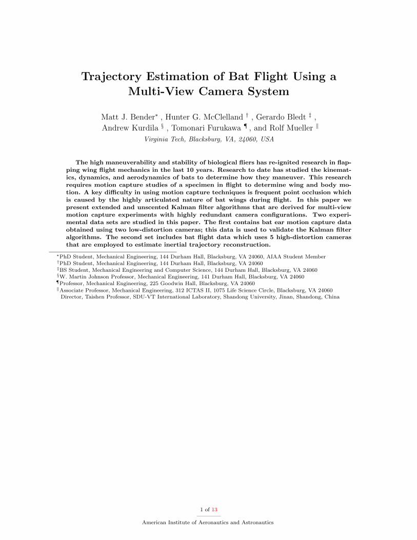
Sample trajectories obtained from the identified motion of the bat wing are depicted in Figure 2a.Figure 2b plots the identified angle motion at the elbow when only a few cameras are used for motionidentification. These plots were created by data obtained from researchers at Brown University as noted in theacknowledgments. This last plot illustrates some of the inherent difficulties that the proposed experimentalfacility has been designed to address. While the overall motion can appear qualitatively correct as in Figure2a, the detailed plot of joint motion illustrates the substantial variance from the mean due to measurementnoise. In addition, substantial portions of the trajectory cannot be identified owing to a lack of observabilityof feature points during some portions of the flight trajectory.

The goal of this research is to derive and test a general methodology for the estimation of fiducial pointmarkers on the wings of bats in flight using a highly redundant, multi-view camera imaging system. Weaccomplish this goal by developing a motion model and sensor model for use in extended and unscented

3 of 13


−40 −20 0 20 −40

−20

0

−20

−10

0

10

Y (cm)

X (cm)

Z (

cm)

Body

Digit 3

Radius

Digit 5

Digit 4

Humerus

(a) Reconstruction of a Bat Wing in Motion

100 200 300 400

−6

−4

−2

0

2

4

Timestep

Angular Displacement (deg) Point Occlusion

(b) Angular Displacement of the Shoulder

Figure 2. Identification of Flapping Motion. Left: A rigid-link, open, kinematic-chain, robotic model has beenfit to the point cloud generated by 3D reconstruction of the motion capture data. Right: One of the identifiedshoulder angles is depicted here. The line is a smooth curve fit for the experimental data. Breaks in this curvefit indicate the regions which could not be identified due to point occlusion.

Kalman filters. We begin in Section II by presenting the full equations of motion of the bat along witha discussion of the difficulties in obtaining various terms in this class of motion models. Then in SectionIII.A we make some simplifying assumptions to arrive at a motion model which is practically implementable.In Section III.B we derive a sensor model which assumes that radial camera distortion is removed priorto incorporation of tracked image points in the Kalman filters. The update laws for the extended andunscented Kalman filters are then presented in Sections III.C and III.D respectively. These filters are usedto perform the seamless data fusion of multiple observations of the fiducial markers to yield estimates ofinertial trajectories.

Our methods are novel due in that they use many low-cost cameras, as opposed to a few high-precisioncameras to estimate bat flight. As discussed previously, for highly occluded motions of bat flight, moreviewing angles are desirable as opposed to more resolution. Ultimately, we wish to understand the kinematicsand dynamics of complex, articulated, multi-body, flapping wing flight and this paper creates a foundationof the numerical methods used to process the raw motion capture footage into inertial trajectories.

II. Dynamics of Bat Flight

While self-occlusion is an inherent issue which makes our problem difficult, bat flight is also difficult tostudy due to complex and uncertain dynamics. The full dynamics of the bat includes complex aerodynamicloads,12 anisotropic wing membrane properties,13 and flexible wing bones.14 To begin modeling bat flight, akey simplifying assumption must be made: the bat bioskeletal system can be represented as a collection ofrigid bodies interconnected by ideal joints. Making this assumption, equations 1 and 2 are prototypical ofmodels that govern the dynamics of a bat in flight

M(θ)θ + C(θ, θ)θ +∂V(θ)

∂θ= τ a(θ, θ) + D(θ)τ c (1)

y = h(θ, θ) (2)

For an n degree of freedom model of bat flight, these equations consist of an n × n nonlinear generalizedmass matrix M(θ), an n×n nonlinear matrix C(θ, θ) used to form centripetal and Coriolis contributions, ascalar potential energy function V (θ), the n−vector τ a(θ, θ) of generalized forces due to aerodynamic loads,the n × n nonlinear control influence matrix D(θ), the input forces and torques τ c, and the n−vector ofgeneralized coordinates θ. The second equation above, Equation 2, expresses how the Cartesian outputs ydepend in a nonlinear fashion on the generalized coordinates θ and their derivatives θ. The specific form of

4 of 13


the entries of Equation 1 has been discussed in control problems15,16 and creation of a bat-inspired roboticmechanism development.17,18

Roughly speaking, the contributions to the equations of motion fall into two categories: geometric andaerodynamic contributions. The mass matrix, centripetal matrix, potential energy, and control influencematrix arise from the underlying problem geometry. That is, these terms can be understood as coordinaterealizations of an evolution law on a suitably defined smooth manifold, and methods for their determinationare well known.19,20 On the other hand, the generalized forces τ a depend inherently on the particular modelused to represent flapping wing aerodynamics. Many alternatives have been studied for these aerodynamiccontributions. An excellent survey of low-order models that have been used to represent aerodynamics offlapping flight mechanics exists.21

In principle, the governing Equations 1 and 2 could used as a motion model for the predictor in a filteringestimate of the inertial trajectories of the fiducial markers. Several issues make an approach based on a directimplementation of this form of the equations of motion intractable. The issues with using this model are thatτ a and τ c are unknown, non-negligible, and un-measureable in real-time. In recent years, computationalfluid dynamics analysis and particle imaging velocimetry (PIV) have been conducted on models of bats andliving specimens to study their aerodynamics. Such studies provide estimates of aerodynamic contributionsfrom computationally intensive batch calculations. These methods are not feasible for on-line estimationof aerodynamic loads. Additionally, EEG and other tests have been conducted to determine control forcesapplied by the muscles during flight maneuvers. Researchers at Brown University have conducted tests whichshow that the stiffness of the wing membrane is actively controlled during flight.22 Like the aerodynamicsstudies, however, the results only give an approximation of the actual values of these controls during flightand, again, are not suitable to build on-line estimates. Since the aerodynamic and control contributionsare significant and unknown, a different motion model will be used for the Kalman filters developed in thispaper.

III. Trajectory Estimation of Bat Flight

Motion tracking has been used widely in recent years to study articulated motion of animals becauseit can estimate posture without the use of mechanical sensors which can constrain motion. Much of thiswork relies on tracking fiducial markers in image space and combining multiple observations using Kalmanor particle filtering.23,24 This section develops the motion and sensor models for Kalman filtering and thenexplicitly details the extended and unscented Kalman filter algorithms.

A. Motion Model

Human motion studies commonly use a random-walk model23,24 due to similar difficulties implementing thefull dynamics as discussed earlier in Section II. For our implementation of Kalman filters for bat flight, weuse a random-walk model as well

xk+1 = xk +w (3)

The motion model does not predict the direction of motion, but rather estimates that the state does notchange dramatically over a typical time step. This is a valid assumption for systems with inertia. Whilethis motion model has a large degree of uncertainty, a conservative estimate for the noise in the system canbe determined by careful study of bats during flight. Our experiment was conducted with great Himalayanleaf-nosed bats (Hipposiderous armiger). The specimen used in this experiment had a wing span of 0.5m.During straight and level flight, flaps its wings at a rate of 4Hz, through an angle of 90 degrees, to createa body velocity of approximately 3ms . The cameras used to capture the motion were recording at 120fps.From this information, we can develop an estimate of the largest motion which will occur between frames.

dm =√d2v + d2f =

√(vffc

)2

+

(αf lwff

1

fc

)2

(4)

In Equation 4, dm is the estimated distance a point can travel, dv is the distance due to forward velocity, dfis the distance due to flapping, vf is the velocity of flight, fc is the camera frame rate, αf is the flap angle,lw is the length of the wingspan, and ff is the frequency of the flap cycle. Assuming this motion is possible

5 of 13


in all directions, there is no cross covariance, and specifying a confidence interval of 95% yields a covarianceof:

Rk =d2m

7.8147I (5)

where I is the n× n identity matrix, and 7.8147 is a scaling factor for a 95% confidence interval in a 3 DOFχ2 cumulative distribution. This covariance is used in the prediction step of the Kalman filters presentedlater. Note that this matrix is constant. The ear motion data uses the same formulation, however, withdifferent characteristic parameter values. The flight speed is zero, ear length is 0.05m, ear motion occurs ata frequency of 10Hz, the ear bends through an angle of 90o, and the camera frame rate is 250fps.

B. Sensor Model

The next portion of the probabilistic filter incorporates the sensor model which will be used for the correctionstep of the algorithm. While the sensor model for a camera is nonlinear, there are well established equationsfor projecting a point in inertial space x into camera pixel coordinates.25 The location of the feature in theimage space φ is known to be

φ =

{ψx

ψy

}=

1

λcKΠ0H

c0x (6)

where λ is the distance from the focal point of the camera to the point x in inertial coordinates, cK is thecamera calibration matrix, Π0 is the canonical projection matrix, and Hc

0 is the homogeneous transformfrom the inertial basis to the camera basis. In our multi-view camera system, the jth camera observation ofthe ith point is thus given by

cjφpi =

cj{ψx

ψy

}pi

=1

cjλpi

cjKΠ0Hcj0 xpi (7)

Given m cameras, all cjφpi will be stacked such that the vector form for all observations of all feature pointsis:

h(xk) =

c1φp1

...

φpn

...

cmφp1

...

φpn

k

=

1

c1λp1,k

c1KΠ0Hc10 xp1,k

...1

c1λpn,k

c1KΠ0Hc10 xpn,k

...

1cmλp1,k

cmKΠ0Hcm0 xp1,k

...1

cmλpn,k

cmKΠ0Hcm0 xpn,k

(8)

In this equation, h is the complete measurement function. As a result, the sensor model in the Kalmanfilters can be expressed with this deterministic model and system noise as

yk = h(xk) + v (9)

The noise vector in this measurement model can be approximated using the errors in the calibrationparameters. The first order approximation of the sensor model covariance is

Qk =∂h(xk)

∂pΣp

∂h(xk)

∂p

T

(10)

where p is the vector of parameters which have uncertainty (e.g. intrinsic and extrinsic parameters of thecalibration), and Σp is a diagonal matrix of parameter covariances. The values for Σp are produced by thecamera calibration.26

Now that we have developed a motion model and sensor model for our experiment, we can present theupdate laws for the extended and unscented Kalman filters.

6 of 13


C. Extended Kalman Filter

The EKF update law is,

xk = Akxk−1 ≡ Mean Prediction (11)

�k = Ak�k−1ATk +Rk ≡ Covariance Prediction (12)

Kk = �kHTk

(Hk�kH

Tk +Qk

)−1

≡ Kalman Gain Calculation (13)

xk = xk +Kk (yk − h(xk)) ≡ State Correction (14)

�k =(I−KkHk

)�k ≡ Covariance Correction (15)

The Jacobian of the sensor model for a single camera measurement of a single point takes the standardform

∂ cjh(xpi)

∂xpi=

1cjλpi

cjKΠ0Hcj0 − cjKΠ0H

cj0 xpi zH

cj0

(zH

cj0 xpi

)−2(16)

where, z =[0 0 1 0

]. The Jacobian for a single camera, which observes multiple points, is then

cjH =

∂ cjh(xp1

)

∂xp10 . . . 0

0. . .

......

. . . 0

0 . . . 0∂ cjh(xpn )∂xpn

(17)

The complete Jacobian for all sensor measurements of all points is:

H =[c1HT ...

cjHT]T

(18)

For this implementation, frequent point occlusions are expected. To account for occlusions, we omit rowsof the sensor model, its Jacobian, and the observation vector. Similarly, we omit rows and columns from thesensor covariance matrix such that the dimensions are consistent. This rescaling procedure eliminates thepoints which are occluded in certain camera views from the correction step of the algorithm. As long as twocameras can view a particular point, the correction will still be meaningful.

D. Unscented Kalman Filter

We wish to compare the performance of the extended Kalman filter to the unscented Kalman filter becausethe latter can often perform better in the presence of non-Gaussian noise or classes of nonlinearities.27 Usingthe same motion model, sensor model, and covariance functions, the UKF update law is,

7 of 13


Xk−1 = UT(xk−1,�k−1) ≡ Unscented Transform of Previous Mean (19)

X∗k = AkXk−1 ≡ Prediction of Sample Points (20)

xk =

2n∑i=0

wm[i](X

∗k[i])

≡ Mean Prediction (21)

�k =

2n∑i=0

wc[i](X

∗k[i] − xk

)(X

∗k[i] − xk

)T+Rk ≡ Covariance Prediction (22)

Xk = UT(xk,�k) ≡ Unscented Transform of Prediction (23)

Yk = H(Xk) ≡ Measurement on Predicted Sample Points (24)

yk =

2n∑i=0

wm[i](Yk[i]

)≡ Measurement Prediction (25)

Sk =

2n∑i=0

wc[i](Yk[i] − yk

) (Yk[i] − yk

)T+Qk ≡ Predicted Measurement Covariance (26)

Kk =

(2n∑i=0

wc[i](Xk[i] − xk

) (Yk[i] − yk

)T)S−1k ≡ Kalman Gain Calculation (27)

xk = xk +Kk (yk − yk) ≡ State Correction (28)

�k = �k −KkSkKTk ≡ Covariance Correction (29)

As in the extended Kalman filter presented above, we account for occlusions by trimming the observationvector yk and reshaping the Kalman gain and sensor covariance matricies, Kk and Qk, respectively.

IV. Results

The EKF and UKF algorithms developed above are applied to two sets of motion capture data: ear motionand straight flapping wing flight. The purpose of considering the ear data is to validate the performanceof the Kalman filters against stereo triangulation performed with data captured using two high qualitycameras. After the performance of the filters is determined for the bat ear data, the results for a flighttrajectory estimation are presented.

A. Bat Ear Data

The first set of motion capture data includes head and ear motions of a great Himalayan leaf-nosed bat(Hipposiderous armiger) echolocating a presented sonar target. The head and ear motion was capturedusing two GigaView cameras having a frame rate of 250 fps and a resolution of 720×1280 pixels. Thesecameras use lenses with minimal lens distortion, so rectification of images was not deemed necessary.

For the ear motion data set, the results of both the EKF and UKF were compared to stereo triangulation.The trajectory reconstruction of all three methods is shown in figure 3a, the error between the EKF and thestereo triangulation is shown in figure 3b, and the error between the UKF and stereo triangulation is shownin figure 3c. The trajectory estimation via the EKF and UKF algorithms are within 1mm of the trajectoriesproduced by the stereo triangulation. Furthermore the errors are approximately constant over the entiredataset. Due to the similarity between the stereo triangulation and Kalman filter reconstructions, we canconclude that the filters converge to the correct trajectory. Furthermore, if the identified trajectories areprojected back into image space, the error between the observation (original point in the image) and theidentified point location can be determined. Figure 4a shows the re-projection of the EKF, UKF, and stereotriangulated trajectories on an original image. Figure 4b, shows the error between these re-projections andthe original image features.

As shown in the figures, all three methods produce re-projections within 5 pixels of the original featurelocations. Note that a 5 pixel reprojection error in image space corresponds to a roughly 2mm uncertaintyin the 3D location of the feature point. Thus, we conclude that the Kalman filter implementation developed

8 of 13


−500

50

−20020490

495

500

505

510

x (mm)

Ear Tip

Ear 3

Ear 1

Ear Points in 3D Coordinates

Ear 4

y (mm)

Ear 2

Head 3

Head 1

Eye

Head 2

z (m

m)

EKFUKFStereo

(a) Ear Marker Inertial Trajectories

2 4 6 8 100

0.5

1

1.5

2

2.5

Timestep

Mag

nitu

de o

f err

or (

mm

)

Error: EKF vs Stereo Triagulation

Ear TipEar 1Ear 2Ear 3Ear 4EyeHead 1Head 2Head 3

(b) Error between EKF and Stereo

2 4 6 8 100

0.5

1

1.5

2

2.5

Timestep

Mag

nitu

de o

f err

or (

mm

)

Error: UKF vs Stereo Triagulation

Ear TipEar 1Ear 2Ear 3Ear 4EyeHead 1Head 2Head 3

(c) Error between UKF and Stereo

Figure 3. EKF, UKF, and stereo triangulation inertial trajectory reconstruction. In (a) the inertial recon-structions using all three methods are shown. In (b) and (c), the error between stereo triangulation and theEKF and UKF reconstructions are shown, respectively. Thus the results of the Kalman filters match the stereoreconstruction well (error < 1mm).

Ear Tip

Ear 1

Ear 2Ear 3

Ear 4

Eye

Head 1

Head 2 Head 3

Image FeaturesStereo ReprojectionEKF ReprojectionUKF Reprojection

(a) Reprojection of Ear Points

−5 0 5−5

0

5

x (pixels)

y (p

ixel

s)

Reprojection Error

EKFUKFStereo

(b) Reprojection Error in Ear Points

Figure 4. Reprojection error of EKF, UKF, and stereo reconstruction methods. The white ear outline in (a)is for visualization only and was not tracked using the outline points. The three head points show minimalmotion which is desirable for studying ear motion. The re-projection error in (b) is within 5 pixels in x and y.

here is satisfactory. This ear motion data was used as an initial training set of data for the development,implementation, and validation of the Kalman filters software and algorithms. The ultimate goal was toproduce inertial trajectory estimates of marker locations for the flapping flight experiments.

B. Bat Flight Data

The second set of data describes the same species of bat flying straight and level through the flight tunnel.The flight motion was recorded with a number of GoPro Hero3+ Black cameras at a frame rate of 120fps and a resolution of 720×1280 pixels. These cameras use the factory lens which contains significantdistortion. The distortion was removed prior to 3D reconstruction using a standard 5 parameter distortionmodel and parameters.28,29,30 For both data sets, feature recognition of fiducial markers was conductedprior to performing inertial trajectory reconstruction.

Two preprocessing steps were necessary before the Kalman filters could be applied to the bat ear motiondata. First radial distortion was removed from the images as mentioned above. Secondly, structure bundleadjustment was performed on the extrinsic parameters computed by the camera calibration toolbox.26 Theinertial trajectories estimated by the Kalman filters are shown in figure 5a. These trajectories are thenprojected into image space and the reprojection error is calculated. Again, this reprojection error is presentedas an uncertainty in the 3D location of the estimated trajectories. Figure 5 plots b-f show the reprojection

9 of 13


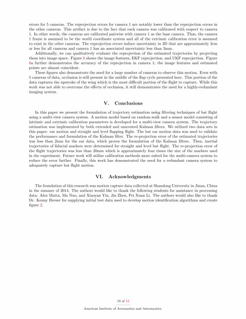
errors for 5 cameras. The reprojection errors for camera 1 are notably lower than the reprojection errors inthe other cameras. This artifact is due to the fact that each camera was calibrated with respect to camera1. In other words, the cameras are calibrated pairwise with camera 1 as the base camera. Thus, the camera1 frame is assumed to be the world coordinate system and all of the extrinsic calibration error is assumedto exist in the other cameras. The reprojection errors induce uncertainty in 3D that are approximately 2cmor less for all cameras and camera 1 has an associated uncertainty less than 3mm.

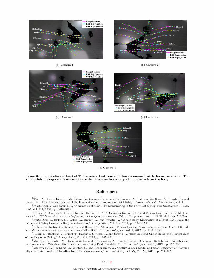
Additionally, we can qualitatively evaluate the reprojection of the estimated trajectories by projectingthem into image space. Figure 6 shows the image features, EKF reprojection, and UKF reprojection. Figure6a further demonstrates the accuracy of the reprojection in camera 1; the image features and estimatedpoints are almost coincident.

These figures also demonstrate the need for a large number of cameras to observe this motion. Even with5 cameras of data, occlusion is still present in the middle of the flap cycle presented here. This portion of thedata captures the upstroke of the wing which is the most difficult portion of the flight to capture. While thiswork was not able to overcome the effects of occlusion, it still demonstrates the need for a highly-redundantimaging system.

V. Conclusions

In this paper we present the formulation of trajectory estimation using filtering techniques of bat flightusing a multi-view camera system. A motion model based on random-walk and a sensor model consisting ofintrinsic and extrinsic calibration parameters is developed for a multi-view camera system. The trajectoryestimation was implemented by both extended and unscented Kalman filters. We utilized two data sets inthis paper: ear motion and straight and level flapping flight. The bat ear motion data was used to validatethe performance and formulation of the Kalman filter. The re-projection error of the estimated trajectorieswas less than 2mm for the ear data, which proves the formulation of the Kalman filters. Then, inertialtrajectories of fiducial markers were determined for straight and level bat flight. The re-projection error ofthe flight trajectories was less than 20mm which is approximately four times the size of the markers usedin the experiment. Future work will utilize calibration methods more suited for the multi-camera system toreduce the error further. Finally, this work has demonstrated the need for a redundant camera system toadequately capture bat flight motion.

VI. Acknowledgments

The foundation of this research was motion capture data collected at Shandong University in Jinan, Chinain the summer of 2014. The authors would like to thank the following students for assistance in processingdata: Alex Matta, Ma Nuo, and Xiaoyan Yin, Jin Zhen, Pei Xuan Li. The authors would also like to thankDr. Kenny Breuer for supplying initial test data used to develop motion identification algorithms and createfigure 2.

10 of 13


−1000

100200

300 −1000

100200

300

400

500

600

700

Digit 4Digit 5

y (mm)

Digit 3

ElbowBody 2

RShoulder

x (mm)

z (m

m)

(a) Inertial Trajectory Reconstruction

−20 −15 −10 −5 0 5 10 15 20−10

−5

0

5

10

15

20

x (mm)

y (m

m)

EKFUKF

(b) Reprojection Error Camera 1

−20 −15 −10 −5 0 5 10 15 20−10

−5

0

5

10

15

20

x (mm)

y (m

m)

EKFUKF

(c) Reprojection Error Camera 2

−20 −15 −10 −5 0 5 10 15 20−10

−5

0

5

10

15

20

x (mm)

y (m

m)

EKFUKF

(d) Reprojection Error Camera 3

−20 −15 −10 −5 0 5 10 15 20−10

−5

0

5

10

15

20

x (mm)

y (m

m)

EKFUKF

(e) Reprojection Error Camera 4

−20 −15 −10 −5 0 5 10 15 20−10

−5

0

5

10

15

20

x (mm)

y (m

m)

EKFUKF

(f) Reprojection Error Camera 6

Figure 5. The inertial trajectories are reconstructed in (a) using both UKF and EKF methods of reconstruction.The blue lines are for visualization of the bat wing. The bat is flying in the negative x direction. Thereprojection errors in each camera are shown in (b) through (f). In these figures the ellipses represents 95%uncertainty ellipses for the EKF (dashed) and UKF (solid) reprojection errors. The re-projection error shownin (b) is less than 3mm while the reprojection errors shown in (c) through (f) are less than 20 mm.

2

11 of 13


Body 2

RShoulder

Elbow

WristDigit 5

Digit 4Digit 3

Image FeaturesEKF ReprojectionUKF Reprojection

(a) Camera 1

Body 2

RShoulder

ElbowWrist

Digit 5

Digit 4

Digit 3


(b) Camera 2

Body 2

RShoulder

Elbow

WristDigit 5

Digit 4

Digit 3


(c) Camera 3

Body 2

RShoulderElbow

Wrist

Digit 5Digit 4

Digit 3


(d) Camera 4

Body 2RShoulder

Elbow

Wrist

Digit 5

Digit 4

Digit 3


(e) Camera 5

Figure 6. Reprojection of Inertial Trajectories. Body points follow an approximately linear trajectory. Thewing points undergo nonlinear motions which increases in severity with distance from the body.

References

1Tian, X., Iriarte-Diaz, J., Middleton, K., Galvao, R., Israeli, E., Roemer, A., Sullivan, A., Song, A., Swartz, S., andBreuer, K., “Direct Measurements of the Kinematics and Dynamics of Bat Flight,” Bioinspiration & Biomimetics, Vol. 1.

2Iriarte-Diaz, J. and Swartz, S., “Kinematics of Slow Turn Maneuvering in the Fruit Bat Cynopterus Brachyotis,” J. Exp.Biol , Vol. 211, 2008, pp. 3478–3489.

3Bergou, A., Swartz, S., Breuer, K., and Taubin, G., “3D Reconstruction of Bat Flight Kinematics from Sparse MultipleViews,” IEEE Computer Science Conference on Computer Vision and Patern Recognition, Vol. 1, IEEE, 2011, pp. 238–245.

4Irarte-Diaz, J., Riskin, D., Willis, D., Breuer, K., and Swartz, S., “Whole-Body Kinematics of a Fruit Bat Reveal theInfluence of Wing Inertia on Body Accelerations,” J. Exp. Biol., Vol. 214, 2011, pp. 1546–1553.

5Hubel, T., Hristov, N., Swartz, S., and Breuer, K., “Changes in Kinematics and Aerodynamics Over a Range of Speedsin Tadarida brasiliensis, the Brazilian Free-Tailed Bat,” J.R. Soc. Interface, Vol. 9, 2012, pp. 1120–1130.

6Riskin, D., Bahlman, J., Hubel, T., Ratcliffe, J., Kunz, T., and Swartz, S., “Bats Go Head-Under-Heels: the Biomechanicsof Landing on a Celing,” J. Exp. Biol., Vol. 212, 2009, pp. 945–953.

7Muijres, F., Bowlin, M., Johansson, L., and Hedenstrom, A., “Vortex Wake, Downwash Distribution, AerodynamicPerformance and Wingbeat Kinematics in Slow-Flying Pied Flycatcher,” J.R. Soc. Interface, Vol. 9, 2012, pp. 292–303.

8Muijres, F. T., Spedding, G., Winter, Y., and Hedenstrom, A., “Actuator Disk Model and Span Efficiency of FlappingFlight in Bats Based on Time-Resolved PIV Measurements,” Journal of Exp. Fluids, Vol. 51, 2011, pp. 511–525.

12 of 13


9Hubel, T., Swartz, D., and Breuer, K., “Wake Structure and Wing Kinematics: The Flight of the Lesser Dog-Faced FruitBat, Cynopterus brachyotis,” J. Exp. Biol., Vol. 213, 2010, pp. 3427–3440.

10Hedenstrom, A., Muijres, F., von Busse, R., Johansson, L., Winter, Y., and Spedding, G., “High Speed Stereo DPIVMeasurement of Wakes of Two Bat Species Flying Freely in a Wind Tunnel,” Journal of Experimental Fluids, Vol. 46, 2009,pp. 923–932.

11Chen, X. and Davis, J., “Camera Placement Considering Occlusion for Robust Motion Caputre,” Stanford UniversityComputer Science Technical Report , 2000.

12Viswanath, K. and Tafti, D. K., “Effect of Stroke Deviation on Forward Flapping Flight,” Vol. 51, 2013, pp. 145–160.13Swartz, S., “Mechanical Properties of Bat Wing Membrane Skin,” Zoology, Vol. 239, 1996, pp. 357–378.14Swartz, S., Skin and Bones: the Mechanical Properties of Bat Wing Tissues, Smithsonian Institution Press, 1998, pp.

109–126.15Bayandor, J., Bledt, G., Dadashi, S., Kurdila, A., Murphy, I., and Lei, Y., “Adaptive control for bioinspired flapping

wing robots,” American Control Conference (ACC), 2013 , June 2013, pp. 609–614.16Dadashi, S., Gregory, J., Lei, Y., Bender, M., Kurdila, A., Bayandor, J., and Muller, R., “Adaptive Control of a Flapping

Wing Robot Inspired by Bat Flight,” AIAA SciTech: Guidance, Navigation, and Control , AIAA, 2014.17Colorado, J., Barrientos, A., Rossi, C., and Breuer, K. S., “Biomechanics of smart wings in a bat robot: morphing wings

using SMA actuators,” Bioinspiration & Biomimetics, Vol. 7, No. 3, 2012, pp. 036006.18Bahlman, J. W., Swartz, S. M., and Breuer, K. S., “Design and characterization of a multi-articulated robotic bat wing,”

Bioinspiration & Biomimetics, Vol. 8, No. 1, 2013, pp. 016009.19Mark W. Spong, Seth Hutchinson, M. V., Robot Modeling and Control .20Bullo, F. and Lewis, A., Geometric Control of Mechanical Systems, Springer, 2004.21Orlowski, C. T. and Girard, A. R., “Modeling and Simulation of Nonlinear Dynamics of Flapping wing Micro Air

Vehicles,” AIAA Journal , Vol. 49, 2011, pp. 969–981.22Swartz, S. M., Groves, M. S., Kim, H. D., and Walsh, W. R., “Mechancial properties of bat wing membrane skin,”

Journal of Zoology, Vol. 239, No. 2, 1996, pp. 357–378.23Hauberg, S., Lauze, F., and Pedersen, K. S., “Unscented Kalman Filtering on Riemannian Manifolds,” Journal of

Mathematical Imaging and Vision, Vol. 46, No. 1, August 2013, pp. 103–120.24Canton-Ferrer, C., Casas, J., and Pardas, M., “Towards a low cost multi-camera marker based human motion capture

system,” Image Processing (ICIP), 2009 16th IEEE International Conference on, Nov 2009, pp. 2581–2584.25Ma, Y., Soatto, S., Koseck, J., and Sastry, S. S., An Invitation to 3-D Vision: From Images to Geometric Models,

Springer, 1st ed., 2004.26Bouguet, J.-Y., “Camera Calibration Toolbox for Matlab,” http://www.vision.caltech.edu/bouguetj/calib_doc/

index.html, Dec. 2013.27Julier, S. J. and Uhlmann, J. K., “A New Extension of the Kalman Filter to Nonlinear Systems,” Proc. SPIE: Signal

Processing, Sensor Fustion, and Target Recognition VI , Vol. 3068, 1997, pp. 182–193.28Zhang, Z., “Flexible camera calibration by viewing a plane from unknown orientations,” Computer Vision, 1999. The

Proceedings of the Seventh IEEE International Conference on, Vol. 1, 1999, pp. 666–673.29Clarke, T. A. and Fryer, J. G., “The Development of Camera Calibration Methods and Models,” The Photogrammetric

Record , Vol. 16, No. 91, 1998, pp. 51–66.30Heikkila, J. and Silven, O., “A four-step camera calibration procedure with implicit image correction,” Computer Vision

and Pattern Recognition, 1997. Proceedings., 1997 IEEE Computer Society Conference on, 1997, pp. 1106–1112.

13 of 13


http://www.vision.caltech.edu/bouguetj/calib_doc/index.html

http://www.vision.caltech.edu/bouguetj/calib_doc/index.html

Trajectory Estimation of Bat Flight Using a Multi-View Camera System

Documents

Transcript of Trajectory Estimation of Bat Flight Using a Multi-View Camera System