Planetary and Space Science 58 (2010) 2044–2049

Contents lists available at ScienceDirect

Planetary and Space Science

0032-06

doi:10.1

� Tel.

E-m

journal homepage: www.elsevier.com/locate/pss

Trajectory and atmospheric structure from entry probes: Demonstration ofa real-time reconstruction technique using a simple direct-to-Earth radio link

Paul Withers �

Center for Space Physics, Boston University, 725 Commonwealth Avenue, Boston, MA 02215, USA

a r t i c l e i n f o

Article history:

Received 19 May 2010

Received in revised form

12 October 2010

Accepted 15 October 2010Available online 23 October 2010

Keywords:

Mars

Atmospheric entry

Accelerometer

Radio science

33/$ - see front matter & 2010 Elsevier Ltd. A

016/j.pss.2010.10.005

: +1 617 353 1531; fax: +1 617 353 6463.

ail address: withers@bu.edu

a b s t r a c t

The reconstruction of the trajectory and atmospheric structure associated with an entry probe has

traditionally relied upon onboard accelerometer measurements. Here we outline an equivalent

reconstruction technique that uses Doppler-shifted direct-to-Earth transmissions instead. A critical

assumption is that the entry probe’s angle of attack is zero. The technique is successfully demonstrated on

the atmospheric entry of the Mars Exploration Rover Opportunity, terminating at parachute deployment.

This technique can be applied in real-time, which supports mission operations and public engagement. It

can also be applied to entry probes that fail during their high-risk atmospheric entry.

& 2010 Elsevier Ltd. All rights reserved.

1. Introduction

Many entry probes maintain a radio link to a receiver whosetrajectory is known and that is capable of recording the frequency ofthe received signals. This receiver can be on Earth, in orbit around theplanetary object that is the target of the entry probe, or flying pastthis planetary object. The trajectory of an entry probe is traditionallyreconstructed from integration of onboard accelerometer measure-ments (Withers and Smith, 2006, and references therein). Oncethe trajectory is obtained, the atmospheric density, pressure, andtemperature along the trajectory can be reconstructed as well(Withers and Smith, 2006, and references therein). Successful recon-struction requires that the accelerometer data is returned to Earth foranalysis. However, the necessary data transmission may not occuruntil some time after atmospheric entry. In the worst case scenario ofa mission that fails during atmospheric entry, the onboard accel-erometer data will be irrevocably lost. In this paper, we use the MarsExploration Rover Opportunity as a case study to investigate whethertrajectory and atmospheric structure associated with an entry probecan be reconstructed from time series of received radio frequencies.Our aim is limited to determining whether or not this concept isviable, thus postponing the development of the concept to a levelsuitable for immediate operational use to future work.

We have identified several reasons why this concept is worthy ofinvestigation. A near-real time trajectory reconstruction provides arapid estimate of landing site location, which is useful for a range of

ll rights reserved.

engineering purposes. It is also useful for the identification of anyanomalous events that may have occurred during entry. A near-real-time atmospheric structure reconstruction provides a rapidassessment of the accuracy of predicted environmental conditions,which is useful for a range of engineering purposes. It also offers atangible data product for engaging the public. Public interest in theatmospheric entry phase of missions is intense, yet few results areavailable until hours or days after entry. If a mission fails duringatmospheric entry (e.g. Beagle 2, Mars Polar Lander), then thistechnique may be able to provide the mission’s only scientific results.

Section 2 introduces the main concept of this work. Section 3outlines how this concept was applied to the atmospheric entry ofOpportunity. Section 4 reports the reconstructed trajectory andatmospheric structure obtained for Opportunity. Section 5 discussesthe implications of this work.

2. Concept

Our objective is to relate the line-of-sight velocity, which can befound from the Doppler shift in the radio signal, to the vectoraerodynamic acceleration. In principle, accomplishment of thisobjective suggests that accelerometer measurements of the aero-dynamic acceleration are no longer needed for trajectory andatmospheric structure reconstruction. However, the establishedaccuracy of reconstructions using accelerometer measurementsmeans that the technique introduced here should be regarded ascomplementary to accelerometer-based techniques. The velocityvector of the entry probe at time t0, v0 , is related to the velocity

0

-2

-4

-6

-8

-10

-12

04:55

:00

04:56

:40

04:58

:20

05:00

:00

05:01

:40

05:03

:20

05:05

:00

05:06

:40

05:08

:20

05:10

:00

Time (UTC)

Gravitational Acceleration

Frictional Deceleration

LOS (Bouncing)

Parachute Deploy

Opportunity EDL Sequencex104+8.434905x109

Sky

Fre

quen

cy (H

z)

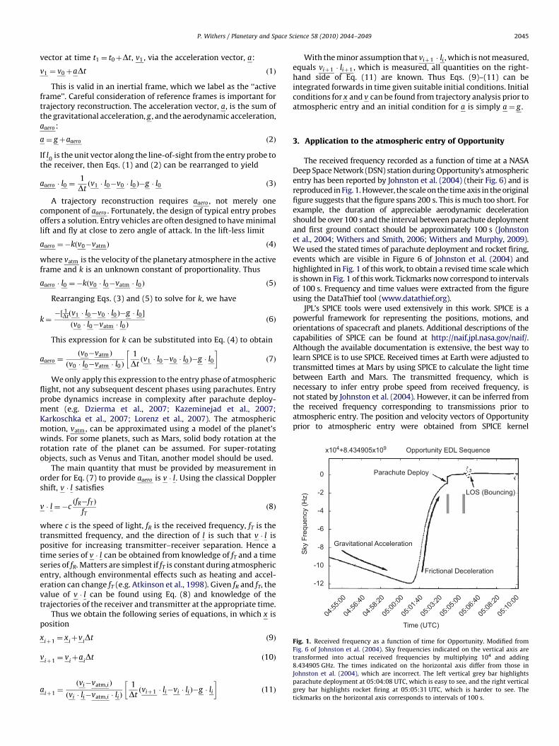
Fig. 1. Received frequency as a function of time for Opportunity. Modified from

Fig. 6 of Johnston et al. (2004). Sky frequencies indicated on the vertical axis are

transformed into actual received frequencies by multiplying 104 and adding

8.434905 GHz. The times indicated on the horizontal axis differ from those in

Johnston et al. (2004), which are incorrect. The left vertical grey bar highlights

parachute deployment at 05:04:08 UTC, which is easy to see, and the right vertical

grey bar highlights rocket firing at 05:05:31 UTC, which is harder to see. The

tickmarks on the horizontal axis corresponds to intervals of 100 s.

P. Withers / Planetary and Space Science 58 (2010) 2044–2049 2045

vector at time t1 ¼ t0þDt, v1 , via the acceleration vector, a:

v1 ¼ v0þaDt ð1Þ

This is valid in an inertial frame, which we label as the ‘‘activeframe’’. Careful consideration of reference frames is important fortrajectory reconstruction. The acceleration vector, a, is the sum ofthe gravitational acceleration, g , and the aerodynamic acceleration,aaero :

a ¼ gþaaero ð2Þ

If l0

is the unit vector along the line-of-sight from the entry probe tothe receiver, then Eqs. (1) and (2) can be rearranged to yield

aaero � l0 ¼1

Dtðv1 � l0�v0 � l0 Þ�g � l0 ð3Þ

A trajectory reconstruction requires aaero , not merely onecomponent of aaero . Fortunately, the design of typical entry probesoffers a solution. Entry vehicles are often designed to have minimallift and fly at close to zero angle of attack. In the lift-less limit

aaero ¼�kðv0�vatm Þ ð4Þ

where vatm is the velocity of the planetary atmosphere in the activeframe and k is an unknown constant of proportionality. Thus

aaero � l0 ¼�kðv0 � l0�vatm � l0 Þ ð5Þ

Rearranging Eqs. (3) and (5) to solve for k, we have

k¼�½ 1Dtðv1 � l0�v0 � l0 Þ�g � l0 �

ðv0 � l0�vatm � l0 Þð6Þ

This expression for k can be substituted into Eq. (4) to obtain

aaero ¼ðv0�vatm Þ

ðv0 � l0�vatm � l0 Þ

�1

Dtðv1 � l0�v0 � l0 Þ�g � l0

�ð7Þ

We only apply this expression to the entry phase of atmosphericflight, not any subsequent descent phases using parachutes. Entryprobe dynamics increase in complexity after parachute deploy-ment (e.g. Dzierma et al., 2007; Kazeminejad et al., 2007;Karkoschka et al., 2007; Lorenz et al., 2007). The atmosphericmotion, vatm , can be approximated using a model of the planet’swinds. For some planets, such as Mars, solid body rotation at therotation rate of the planet can be assumed. For super-rotatingobjects, such as Venus and Titan, another model should be used.

The main quantity that must be provided by measurement inorder for Eq. (7) to provide aaero is v � l. Using the classical Dopplershift, v � l satisfies

v � l ¼�cðfR�fT Þ

fTð8Þ

where c is the speed of light, fR is the received frequency, fT is thetransmitted frequency, and the direction of l is such that v � l ispositive for increasing transmitter–receiver separation. Hence atime series of v � l can be obtained from knowledge of fT and a timeseries of fR. Matters are simplest if fT is constant during atmosphericentry, although environmental effects such as heating and accel-eration can change fT (e.g. Atkinson et al., 1998). Given fR and fT, thevalue of v � l can be found using Eq. (8) and knowledge of thetrajectories of the receiver and transmitter at the appropriate time.

Thus we obtain the following series of equations, in which x isposition

xiþ1¼ x

iþv

iDt ð9Þ

viþ1¼ v

iþa

iDt ð10Þ

aiþ1¼

ðvi�vatm,i Þ

ðvi � li�vatm,i � li Þ

�1

Dtðviþ1 � li�vi � li Þ�g � li

�ð11Þ

With the minor assumption that viþ1 � li , which is not measured,equals viþ1 � liþ1 , which is measured, all quantities on the right-hand side of Eq. (11) are known. Thus Eqs. (9)–(11) can beintegrated forwards in time given suitable initial conditions. Initialconditions for x and v can be found from trajectory analysis prior toatmospheric entry and an initial condition for a is simply a ¼ g .

3. Application to the atmospheric entry of Opportunity

The received frequency recorded as a function of time at a NASADeep Space Network (DSN) station during Opportunity’s atmosphericentry has been reported by Johnston et al. (2004) (their Fig. 6) and isreproduced in Fig. 1. However, the scale on the time axis in the originalfigure suggests that the figure spans 200 s. This is much too short. Forexample, the duration of appreciable aerodynamic decelerationshould be over 100 s and the interval between parachute deploymentand first ground contact should be approximately 100 s (Johnstonet al., 2004; Withers and Smith, 2006; Withers and Murphy, 2009).We used the stated times of parachute deployment and rocket firing,events which are visible in Figure 6 of Johnston et al. (2004) andhighlighted in Fig. 1 of this work, to obtain a revised time scale whichis shown in Fig. 1 of this work. Tickmarks now correspond to intervalsof 100 s. Frequency and time values were extracted from the figureusing the DataThief tool (www.datathief.org).

JPL’s SPICE tools were used extensively in this work. SPICE is apowerful framework for representing the positions, motions, andorientations of spacecraft and planets. Additional descriptions of thecapabilities of SPICE can be found at http://naif.jpl.nasa.gov/naif/.Although the available documentation is extensive, the best way tolearn SPICE is to use SPICE. Received times at Earth were adjusted totransmitted times at Mars by using SPICE to calculate the light timebetween Earth and Mars. The transmitted frequency, which isnecessary to infer entry probe speed from received frequency, isnot stated by Johnston et al. (2004). However, it can be inferred fromthe received frequency corresponding to transmissions prior toatmospheric entry. The position and velocity vectors of Opportunityprior to atmospheric entry were obtained from SPICE kernel

-250 -200 -150 -100 -50 0Time with respect to parachute deployment (sec)

0.01

0.10

1.00

10.00

100.00

Aer

odyn

amic

acc

eler

atio

n (m

s-2

)

Fig. 2. Aerodynamic acceleration determined in this work (black line) and from

Withers and Murphy (2009) (grey line) as functions of time.

-250 -200 -150 -100 -50 0Time with respect to parachute deployment (sec)

0

1000

2000

3000

4000

5000

6000

Atm

osph

ere-

rela

tive

spee

d (m

s-1

)

Fig. 3. Atmosphere-relative speed ðjv0�vatm jÞ determined in this work (black line)

and from Withers and Murphy (2009) (grey line) as functions of time. Relative to the

centre of mass of Mars, the magnitude of vatm is two hundred metres per second.

P. Withers / Planetary and Space Science 58 (2010) 2044–20492046

spk_b_c_030708-040125_recon.bsp for the desired times usingstandard SPICE tools. The trajectory of the receiver depends on whichDSN station recorded the data reported by Johnston et al. (2004). Thespeed of Earth relative to Opportunity at entry is about 19.30 km s�1.Using different DSN locations alters this value by 0.15 km s�1 or lessthan 1%, which is not very large for the accuracies desired in this work,so a receiver location at Earth’s centre of mass was assumed. SPICEtools were used to find the state vectors (position and velocity) ofOpportunity and the receiver in an inertial frame at the desired times,from which the line-of-sight speed of Opportunity relative tothe receiver was determined. Calculation of the Doppler shiftassociated with this speed showed that the transmitted frequencywas 8.4353524 GHz. This frequency was assumed to remain constantthroughout entry. Note that the frequency of 8.434905 GHz indicatedin Fig. 1 corresponds to Opportunity at rest on the surface of Mars,when the transmitter is moving relative to the receiver at severalkm s�1 due to the motions of Earth and Mars. Hence 8.434905 GHz isnot the transmitted frequency. The unit vectors introduced in Section2 were found from the calculated position vectors of Opportunity andthe receiver.

The time series of received frequencies were then processed togive a series of line-of-sight speeds of Opportunity relative to thereceiver as a function of transmission time at Mars. The integrationof Eqs. (9)–(11) was performed in a Mars-fixed reference frame.Accordingly, the line-of-sight speed of the centre of mass ofMars relative to the receiver was subtracted from the line-of-sight speed of Opportunity relative to the receiver to give theline-of-sight speed of Opportunity relative to the centre of massof Mars.

The UTC start time for the trajectory reconstruction was 2004JAN 25 04:48:41.711, corresponding to a radial distance fromMars of 3522.2 km. This was the distance defined by the MarsExploration Rover project as the atmospheric entry interface(Kass et al., 2004). The initial position and velocity of Opportunityin a Mars-fixed reference frame were obtained using SPICE toolsand the initial aerodynamic acceleration was set to zero. Thegravitational acceleration was calculated using an inverse-squarelaw with GM¼ 4:2828� 104 km3 s�2 (Lodders and Fegley, 1998).The trajectory reconstruction was terminated at parachutedeployment.

-250 -200 -150 -100 -50 0

Time with respect to parachute deployment (sec)

0

50

100

150

Alti

tude

(km

)

Fig. 4. Altitude determined in this work (black line) and from Withers and Murphy

(2009) (grey line) as functions of time.

4. Results

A reconstruction of the trajectory and atmospheric structureassociated with Opportunity has already been performed usingonboard accelerometer data. Scientific results are reported inWithers and Smith (2006) and the data products are archived inWithers and Murphy (2009).

Fig. 2 shows the magnitude of the reconstructed aerodynamicacceleration as a function of time, and includes comparisons to theresults of Withers and Murphy (2009). The inferred values ofaerodynamic acceleration are reasonable for approximately 200 spreceding parachute deployment. The peak deceleration found inthis work, 62.5 m s�2, is within 2% of the value reported by Withersand Murphy (2009), 61.5 m s�2.

Figs. 3 and 4 show the reconstructed atmosphere-relative speedand altitude as functions of time, and include comparisons to theresults of Withers and Murphy (2009). All altitudes used in thiswork are radial distances above the landing site at 3394.1 km. Thespeed at parachute deployment found in this work, 596 m s�1, isover 35% greater than the value reported by Withers and Murphy(2009), 430 m s�1, but this difference of 166 m s�1 is only 3% of theatmosphere-relative speed at entry of 5.5 km s�1. The altitude atparachute deployment found in this work, 5.0 km, is less than thevalue reported by Withers and Murphy (2009), 6.2 km, but this

difference is only 1% of the vertical distance between atmosphericentry and parachute deployment.

Fig. 5 shows the individual components of the reconstructedatmosphere-relative velocity. Opportunity’s motion is predominantly

-3.0 -2.8 -2.6 -2.4 -2.2 -2.0 -1.80

50

100

150

Alti

tude

(km

)

Latitude (°N)

P. Withers / Planetary and Space Science 58 (2010) 2044–2049 2047

eastward and the vertical descent speed is on the order of500–1000 m s�1. Figs. 6–8 show the reconstructed atmosphere-relative speed, latitude, and longitude, respectively, as functions ofaltitude, and include comparisons to the results of Withers andMurphy (2009). Differences in speed are only apparent below20 km. Differences in latitude and longitude are minor. The differencesin latitude and longitude at parachute deployment are 0.011 and 0.31,respectively. Again, differences in longitude are only apparent below20 km.

Since the reconstructed aerodynamic acceleration is unreliable athigh altitudes, the atmospheric structure reconstruction commencedat 80 km altitude. This used the traditional approach adopted bymany previous workers (Withers and Smith, 2006, and referencestherein). Atmospheric density, r, is related to the magnitude of theaerodynamic acceleration (Magalh~aes et al., 1999):

mjaaeroj ¼rAðv�vatm Þ

2C

2ð12Þ

-2000 0 2000 4000 6000Atmosphere-relative velocity (m s-1)

0

50

100

150

Alti

tude

(km

)

Fig. 5. Components of the atmosphere-relative velocity, v0�vatm . The solid line is

the zonal component, positive eastward. The dotted line is the radial component,

positive upwards. The dashed line is the meridional component, positive south-

wards. The vertical grey line indicates zero velocity.

0 1000 2000 3000 4000 5000 6000

Atmosphere-relative speed (m s-1)

0

50

100

150

Alti

tude

(km

)

Fig. 6. Atmosphere-relative speed ðjv0�vatm jÞ determined in this work (black line)

and from Withers and Murphy (2009) (grey line) as functions of altitude. Relative to

the centre of mass of Mars, the magnitude of vatm is two hundred metres per second.

Fig. 7. Latitude determined in this work (black line) and from Withers and Murphy

(2009) (grey line) as functions of altitude.

340 345 350 3550

50

100

150

Alti

tude

(km

)

Longitude (°E)

Fig. 8. Longitude determined in this work (black line) and from Withers and

Murphy (2009) (grey line) as functions of altitude.

where m is the spacecraft mass (832.2 kg—Desai and Knocke, 2004),A is the reference area of the spacecraft (disk of diameter2.648 m—Schoenenberger et al., 2005), and C is an aerodynamiccoefficient, which is usually on the order of 2 (Withers et al., 2003).The aerodynamic coefficients needed to relate density to aerody-namic acceleration were obtained from the aerodynamic databasepublished by Schoenenberger et al. (2005) assuming that the angle ofattack was always zero. Atmospheric pressure, p, is related torby theequation of hydrostatic equilibrium:

dp

dr¼�rg ð13Þ

where g is the magnitude of the gravitational acceleration introducedin Section 3 and r is distance from the centre of mass. Atmospherictemperature, T, is related to r and p by the ideal gas law:

mp¼ r R

NAT ð14Þ

where m¼ 43:49 g mol�1 is the mass of one mole of the martianatmosphere, R is the universal gas constant, and NA is Avogrado’snumber (Magalh~aes et al., 1999). A temperature of 120 K wasassumed at the upper boundary to provide a boundary conditionfor the equation of hydrostatic equilibrium. The Knudsen (Kn) and

0 100 200 300 400Temperature (K)

0

20

40

60

80

Alti

tude

(km

)

Fig. 11. Temperature determined in this work (black line) and from Withers and

Murphy (2009) (grey line) as functions of altitude.

P. Withers / Planetary and Space Science 58 (2010) 2044–20492048

Mach (Ma) numbers were also calculated. Kn is defined as

Kn¼1ffiffiffi

2p

pd2nDð15Þ

where d is the diameter of an atmospheric molecule (4.64�10�10 m—Schoenenberger et al., 2005), n, which satisfies n¼

NAr=m, is the atmospheric number density, and D is the diameterof the entry probe. Ma is defined as

Ma¼jv�vatm j

ðgp=rÞ1=2ð16Þ

where g is the ratio of the heat capacity at constant pressure to theheat capacity at constant volume of the martian atmosphere (7/5 foran ideal linear polyatomic gas like CO2—Atkins, 2002). Reconstructeddensity, pressure, temperature, Kn, and Ma are shown in Figs. 9–13 asfunctions of altitude and compared to the results of Withers andMurphy (2009). Results in Figs. 9–13 have been smoothed to reducehigh frequency oscillations. The plotted value at a particular altitudeis the mean (arithmetic mean for temperature and Ma, geometricmean for density, pressure, and Kn) of all results within 75 km ofthat altitude.

Density differences are o20% between 20 and 70 km. Pressuredifferences are o20% between 15 and 70 km. Temperature

10-6

Density (kg m-3)

0

20

40

60

80

Alti

tude

(km

)

10-5 10-4 10-3 10-2

Fig. 9. Density determined in this work (black line) and from Withers and Murphy

(2009) (grey line) as functions of altitude.

0.01 0.1 1 10 100Pressure (Pa)

0

20

40

60

80

Alti

tude

(km

)

Fig. 10. Pressure determined in this work (black line) and from Withers and Murphy

(2009) (grey line) as functions of altitude.

10-6 10-5 10-4 10-3 10-2

Kn

0

20

40

60

80A

ltitu

de (k

m)

Fig. 12. Knudsen number (Kn) determined in this work (black line) and from

Withers and Murphy (2009) (grey line) as functions of altitude.

0 10 20 30 40Ma

0

20

40

60

80

Alti

tude

(km

)

Fig. 13. Mach number (Ma) determined in this work (black line) and from Withers

and Murphy (2009) (grey line) as functions of altitude.

P. Withers / Planetary and Space Science 58 (2010) 2044–2049 2049

differences are o30 K between 20 and 80 km, although theyexceed 100 K close to parachute deployment. Knudsen differencesare o20% between 20 and 70 km, although they exceed 50% below15 km. Mach differences are o20% at all altitudes above 10 km.The tendency for increased errors at low altitude can be attributedto the large relative difference between the atmosphere-relativespeed found in this work and in Withers and Murphy (2009).

5. Discussion

This work used the atmospheric entry of Opportunity as acase study to show that the concept of using Doppler-shifteddirect-to-Earth transmissions to perform real-time trajectory andatmospheric structure reconstructions for entry probes is viable.The trajectory and atmospheric structure found for Opportunity inthis work compare well with the results of analysis of acceler-ometer data from its atmospheric entry. Upcoming missions thatmight benefit from this technique include Mars Science Laboratory(2011 launch), ESA’s Mars EDL technology demonstrator that willaccompany the Mars Trace Gas Orbiter (2016 launch), subsequentMars landers, and entry probes for Venus, Titan and the giantplanets.

Although a detailed error analysis is not appropriate for thispreliminary concept study, it is clear that many of the differencesbetween the results of this work and those of Withers and Murphy(2009) can be attributed to the relatively crude data used here. If thistechnique were applied realistically, then knowledge of the trans-mitted frequency, times, and received frequencies would be signifi-cantly better than was possible for this work. Two steps are necessarybefore this technique can be relied upon to support future entryprobes formally. First, it should be demonstrated using actual receivedfrequencies, not values extracted from a published figure. Possible testcases include the Pioneer Venus probes (Counselman et al., 1980),Pathfinder (Wood et al., 1997), Spirit, Opportunity, Phoenix (Kornfeldet al., 2008), and the Galileo probe (Atkinson et al., 1998). Second,sensitivity studies and error analyses should be performed to quantifythe expected accuracy of its results.

Acknowledgements

P.W. acknowledges Mike Bird and an anonymous reviewer, aswell as fruitful discussions with many colleagues in the planetaryentry probe and radio science communities.

References

Atkins, P.W., 2002. Physical Chemistry, sixth ed. W.H. Freeman,.Atkinson, D.H., Pollack, J.B., Seiff, A., 1998. The Galileo probe Doppler wind

experiment: measurement of the deep zonal winds on Jupiter. J. Geophys.

Res. 103, 22911–22928.Counselman, C.C., Gourevitch, S.A., King, R.W., Loriot, G.B., Ginsberg, E.S., 1980. Zonal

and meridional circulation of the lower atmosphere of Venus determined byradio interferometry. J. Geophys. Res. 85, 8026–8030.

Desai, P.N., Knocke, P.C., 2004. Mars Exploration Rover entry, descent, and landingtrajectory analysis. In: American Institute of Aeronautics and Astronautics paper2004-5092, 42nd AIAA Aerospace Science Meeting in Reno, Nevada, USA.

Dzierma, Y., Bird, M.K., Dutta-Roy, R., Perez-Ayucar, M., Plettemeier, D., Edenhofer,P., 2007. Huygens probe descent dynamics inferred from channel B signal level

measurements. Planet. Space Sci. 55 (November), 1886–1895.Johnston, D., Asmar, S.W., Chang, C., Estabrook, P., Finely, S., Pham, T., Satorius, E.,

2004. Radio science receiver support of the Mars Exploration Rover landings. In:Third ESA International Workshop on Tracking, Telemetry and CommandSystems for Space Applications, Darmstadt, Germany, available online at

/http://hdl.handle.net/2014/39097S.Karkoschka, E., Tomasko, M.G., Doose, L.R., See, C., McFarlane, E.A., Schroder, S.E.,

Rizk, B., 2007. DISR imaging and the geometry of the descent of the Huygensprobe within Titan’s atmosphere. Planet. Space Sci. 55, 1896–1935.

Kass, D.M., Schofield, J.T., Crisp, J., Bailey, E.S., Konefat, E.H., Lee, W.J., Litty, E.C.,Manning, R.M., San Martin, A.M., Willis, R.J., Beebe, R.F., Murphy, J.R., Huber, L.F.,2004. PDS volume MERIMU_0001. In: MER1/MER2-M-IMU-4-EDL-V1.0, NASA

Planetary Data System.Kazeminejad, B., Atkinson, D.H., Perez-Ayucar, M., Lebreton, J., Sollazzo, C., 2007.

Huygens’ entry and descent through titan’s atmosphere—methodology andresults of the trajectory reconstruction. Planet. Space Sci. 55, 1845–1876.

Kornfeld, R.P., Garcia, M.D., Craig, L.E., Butman, S., Signori, G.M., 2008. Entry, descent,and landing communications for the 2007 Phoenix Mars lander. J. SpacecraftRockets 45, 534–547.

Lodders, K., Fegley, B., 1998. The Planetary Scientist’s Companion. Oxford UniversityPress.

Lorenz, R.D., Zarnecki, J.C., Towner, M.C., Leese, M.R., Ball, A.J., Hathi, B., Hagermann,A., Ghafoor, N.A.L., 2007. Descent motions of the Huygens probe as measured by

the surface science package (SSP): turbulent evidence for a cloud layer. Planet.Space Sci. 55, 1936–1948.

Magalh~aes, J.A., Schofield, J.T., Seiff, A., 1999. Results of the Mars Pathfinderatmospheric structure investigation. J. Geophys. Res. 104, 8943–8956.

Schoenenberger, M., Cheatwood, F.M., Desai, P.N., 2005. Static aerodynamics of theMars Exploration Rover entry capsule. In: American Institute of Aeronautics andAstronautics paper 2005-0056, 43rd AIAA Aerospace Science Meeting in Reno,

Nevada, USA.Withers, P., Murphy, J.R., 2009. PDS volume MERIMU_0002. In: MER1/MER2-M-

IMU-5-EDL-DERIVED-V1.0, NASA Planetary Data System.Withers, P., Smith, M.D., 2006. Atmospheric entry profiles from the Mars Exploration

Rovers spirit and opportunity. Icarus 185, 133–142.Withers, P., Towner, M.C., Hathi, B., Zarnecki, J.C., 2003. Analysis of entry accel-

erometer data: a case study of Mars Pathfinder. Planet. Space Sci. 51, 541–561.Wood, G.E., Asmar, S.W., Rebold, T.A., Lee, R.A., 1997. Mars Pathfinder entry, descent,

and landing communications. JPL TDA Progress Report 42–131, available online

at /http://ipnpr.jpl.nasa.gov/progress_report/42-131/131I.pdfS.