TRAINING ON COMPUTABLE

GENERAL EQUILIBRIUM MODELLING

MODEL AUTA

A CLOSED ECONOMY WITHOUT

GOVERNMENT

This pedagogical material was developed by Véronique Robichaud and

accompanies Lesson 5. The model used is an adaptation of the model AUTA

presented in: Decaluwé, B., A. Martens and L. Savard (2001), « La politique

économique du développement et les modèles d'équilibre général calculable.

Une introduction », Montréal, Presses de l'Université de Montréal, 524 p. Since the

SAM has been changed, the simulation results cannot be compared.

1

Table of content

Hypotheses ........................................................................................................................ 2

Sets ...................................................................................................................................... 2

Equations ........................................................................................................................... 3

Variables ............................................................................................................................ 5

Parameters ........................................................................................................................ 6

The social accounting matrix for AUTA ......................................................................... 7

Correspondence between the SAM and the model ................................................. 8

Schema .............................................................................................................................. 9

GAMS Code .................................................................................................................... 10

Value of parameters ...................................................................................................... 17

Simulations ....................................................................................................................... 18

2

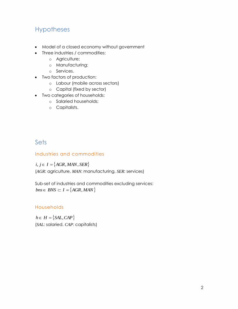
Hypotheses

Model of a closed economy without government

Three industries / commodities:

o Agriculture;

o Manufacturing;

o Services.

Two factors of production:

o Labour (mobile across sectors)

o Capital (fixed by sector)

Two categories of households:

o Salaried households;

o Capitalists.

Sets

Industries and commodities

SERMANAGRIji ,,,

(AGR: agriculture, MAN: manufacturing, SER: services)

Sub-set of industries and commodities excluding services:

MANAGRIBNSbns ,

Households

CAPSALHh ,

(SAL: salaried, CAP: capitalists)

3

Equations

Production Number of equations

1. jjj XSvVA 3

2. jjj XSioCI 3

3. jj

jjjj KDLDAVA

1

3

4. W

VAPVALD

jjj

j

3

5.

j

jjj

jR

VAPVAKD

1 3

6. jjiji CIaijDI ,, 9

Income and savings

7. j

jSAL LDWYH '' 1

8. DIVKDRYHj

jjCAP '' 1

9. hhh YHSH 2

10. hhh SHYHCTH 2

11. j

jj KDRYF 1 1

12. DIVYFSF 1

Demand

13. i

hhi

hiP

CTHC

,

,

6

14. i

ii

P

ITINV

3

15. j

jii DIDIT , 3

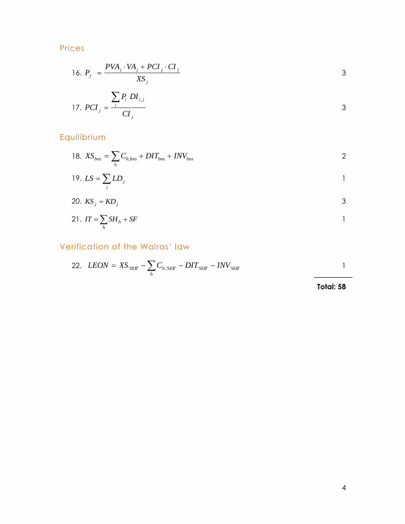
4

Prices

16. j

jjjj

jXS

CIPCIVAPVAP

3

17. j

i

jii

jCI

DIP

PCI

,

3

Equil ibrium

18. bnsbns

h

bnshbns INVDITCXS , 2

19. j

jLDLS 1

20. jj KDKS 3

21. SFSHITh

h 1

Verification of the Walras’ law

22. ''''',''' SERSER

h

SERhSER INVDITCXSLEON 1

Total: 58

5

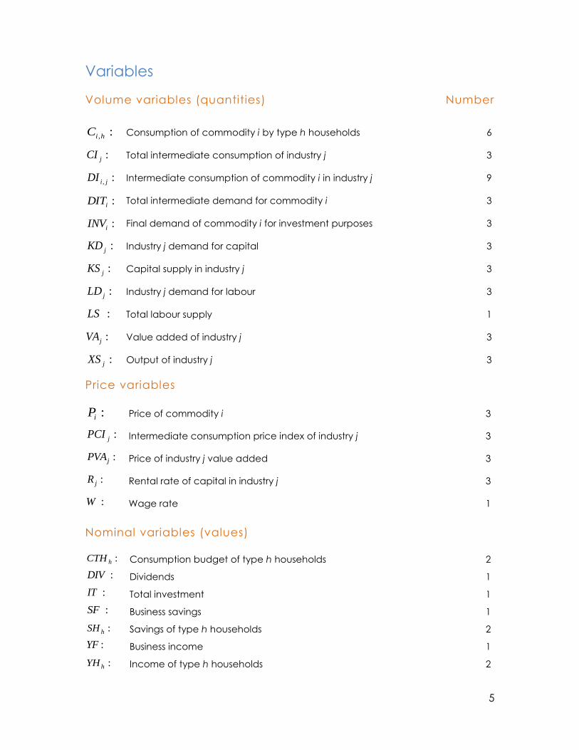
Variables

Volume variables (quantities) Number

:,hiC Consumption of commodity i by type h households 6

:jCI Total intermediate consumption of industry j 3

:, jiDI Intermediate consumption of commodity i in industry j 9

:iDIT Total intermediate demand for commodity i 3

:iINV Final demand of commodity i for investment purposes 3

:jKD Industry j demand for capital 3

:jKS Capital supply in industry j 3

:jLD Industry j demand for labour 3

:LS Total labour supply 1

:jVA Value added of industry j 3

:jXS Output of industry j 3

Price variables

:iP Price of commodity i 3

:jPCI Intermediate consumption price index of industry j 3

:jPVA Price of industry j value added 3

:jR Rental rate of capital in industry j 3

:W Wage rate 1

Nominal variables (values)

:hCTH Consumption budget of type h households 2

:DIV Dividends 1

:IT Total investment 1

:SF Business savings 1

:hSH Savings of type h households 2

:YF Business income 1

:hYH Income of type h households 2

6

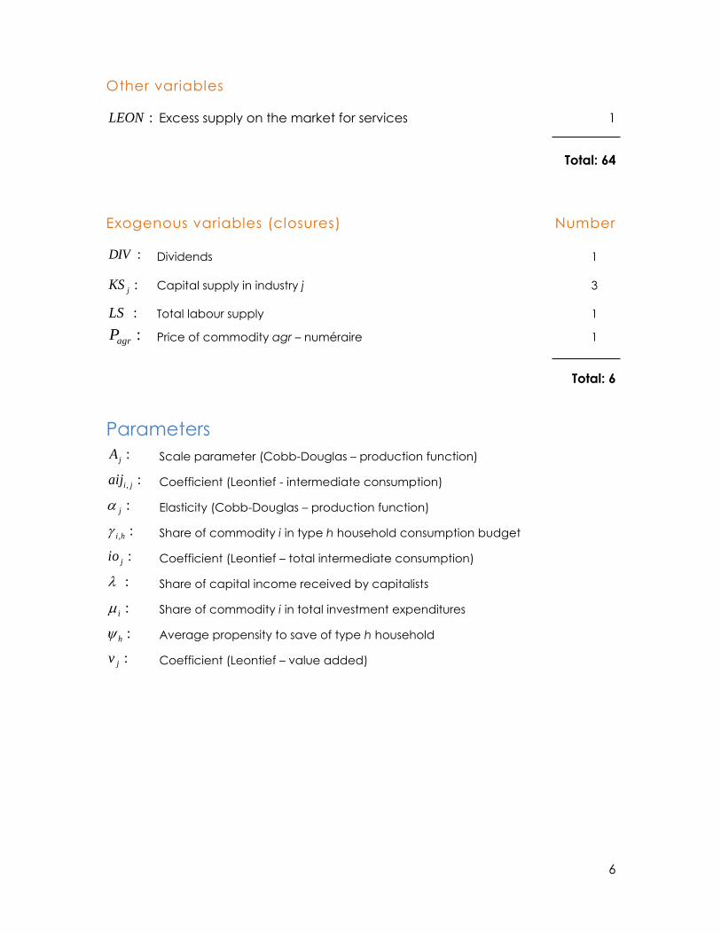
Other variables

:LEON Excess supply on the market for services 1

Total: 64

Exogenous variables (closures) Number

:DIV Dividends 1

:jKS Capital supply in industry j 3

:LS Total labour supply 1

:agrP Price of commodity agr – numéraire 1

Total: 6

Parameters

:jA Scale parameter (Cobb-Douglas – production function)

:, jiaij Coefficient (Leontief - intermediate consumption)

:j Elasticity (Cobb-Douglas – production function)

:,hi Share of commodity i in type h household consumption budget

:jio Coefficient (Leontief – total intermediate consumption)

: Share of capital income received by capitalists

:i Share of commodity i in total investment expenditures

:h Average propensity to save of type h household

:jv Coefficient (Leontief – value added)

7

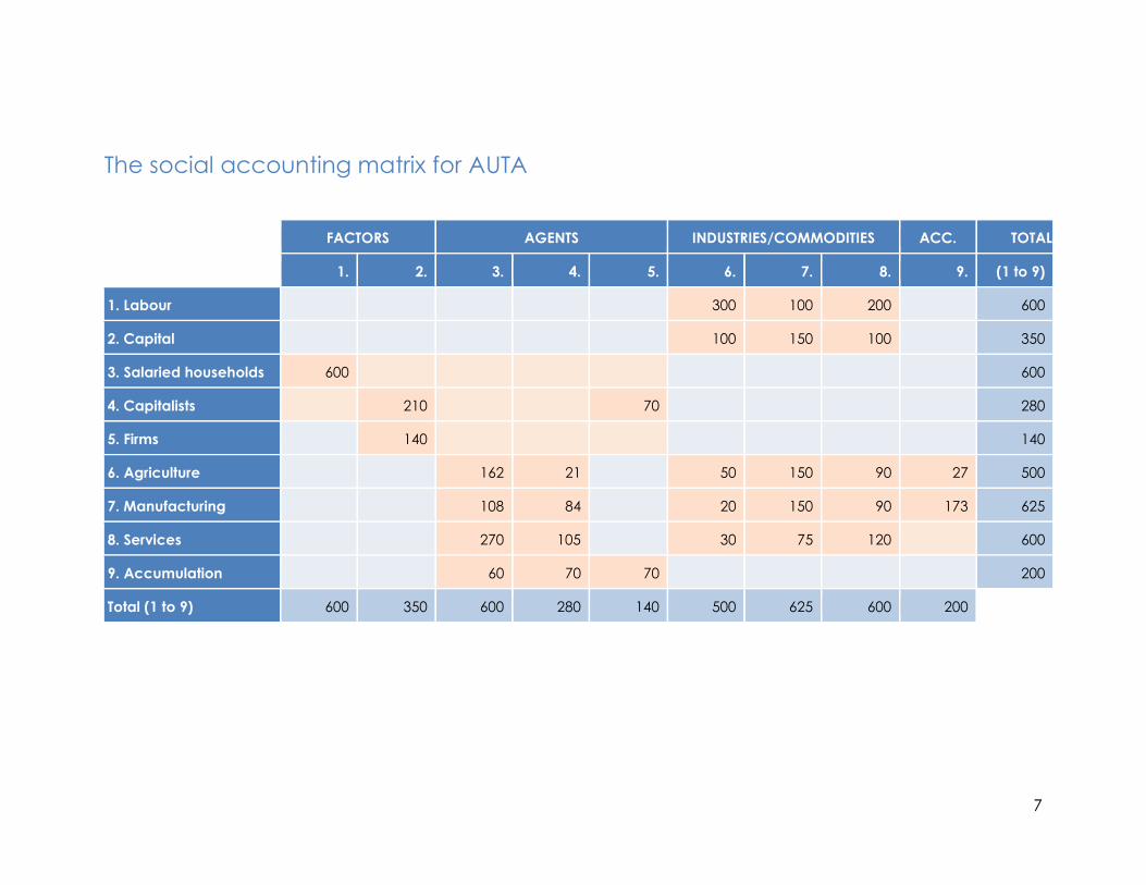
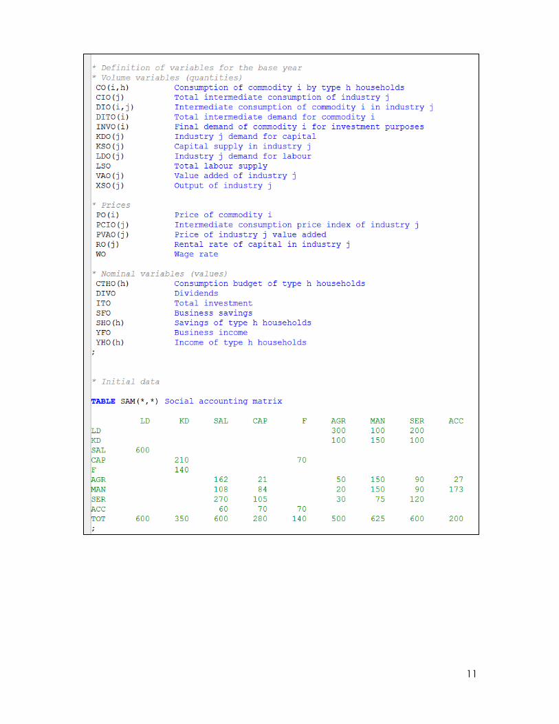
The social accounting matrix for AUTA

FACTORS AGENTS INDUSTRIES/COMMODITIES ACC. TOTAL

1. 2. 3. 4. 5. 6. 7. 8. 9. (1 to 9)

1. Labour 300 100 200 600

2. Capital 100 150 100 350

3. Salaried households 600 600

4. Capitalists 210 70 280

5. Firms 140 140

6. Agriculture 162 21 50 150 90 27 500

7. Manufacturing 108 84 20 150 90 173 625

8. Services 270 105 30 75 120 600

9. Accumulation 60 70 70 200

Total (1 to 9) 600 350 600 280 140 500 625 600 200

8

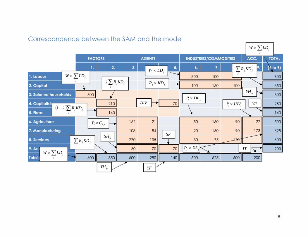
Correspondence between the SAM and the model

FACTORS AGENTS INDUSTRIES/COMMODITIES ACC. TOTAL

1. 2. 3. 4. 5. 6. 7. 8. 9. (1 to 9)

1. Labour 300 100 200 600

2. Capital 100 150 100 350

3. Salaried households 600 600

4. Capitalists 210 70 280

5. Firms 140 140

6. Agriculture 162 21 50 150 90 27 500

7. Manufacturing 108 84 20 150 90 173 625

8. Services 270 105 30 75 120 600

9. Accumulation 60 70 70 200

Total (1 to 9) 600 350 600 280 140 500 625 600 200

j

jLDW jLDW

jj KDR

j

jLDW

j

jjKDR

j

jj KDR1

j

jLDW

tr

trtr KDR

j

jj KDR

j

jj KDR

DIV

hYH

hYH

hSH

hii CP ,

SF

YF

YF jii DIP ,

jj XSP

ii INVP

IT

9

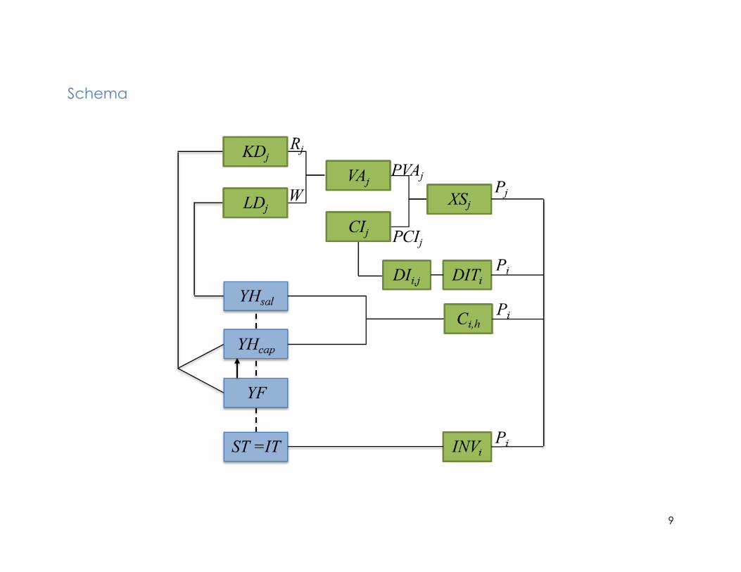
Schema

10

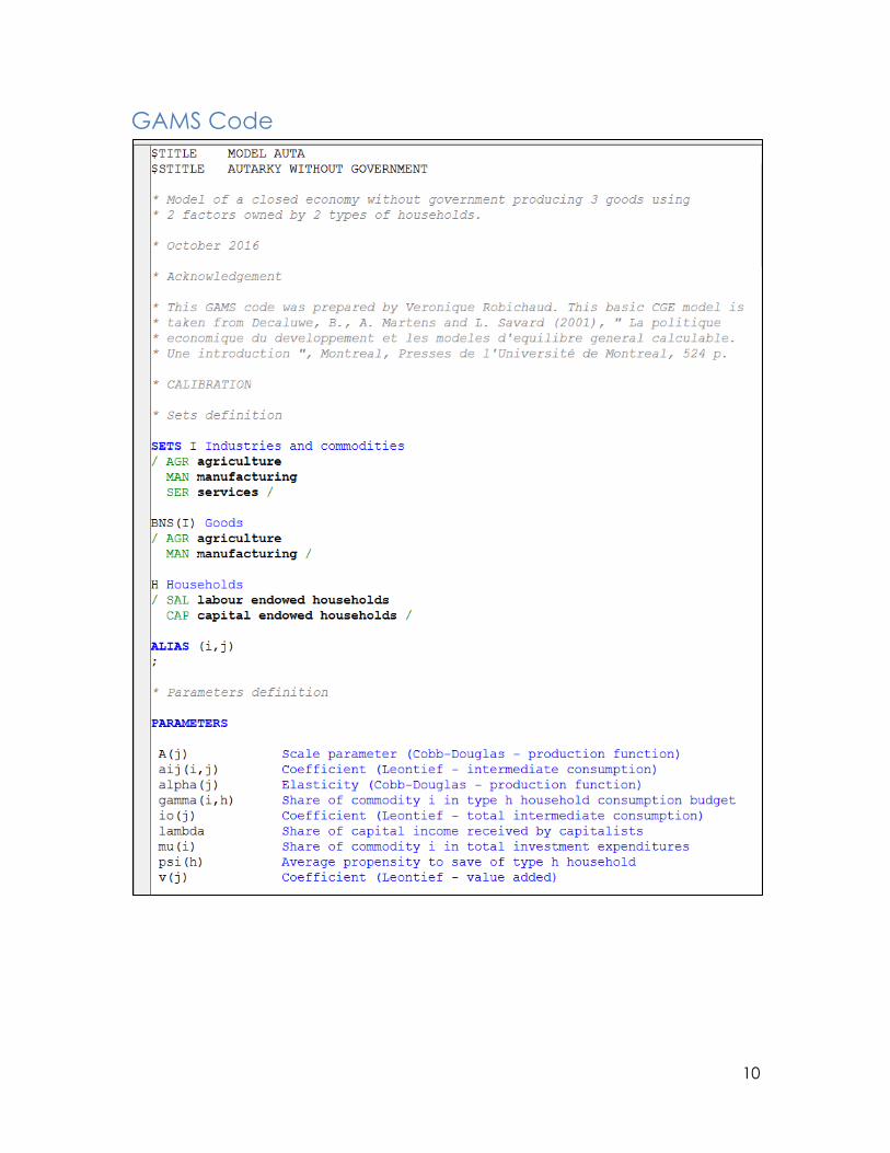
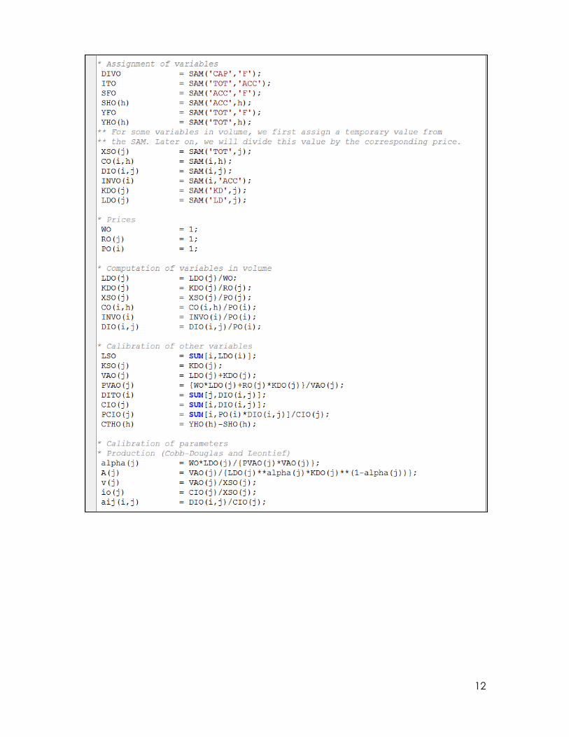
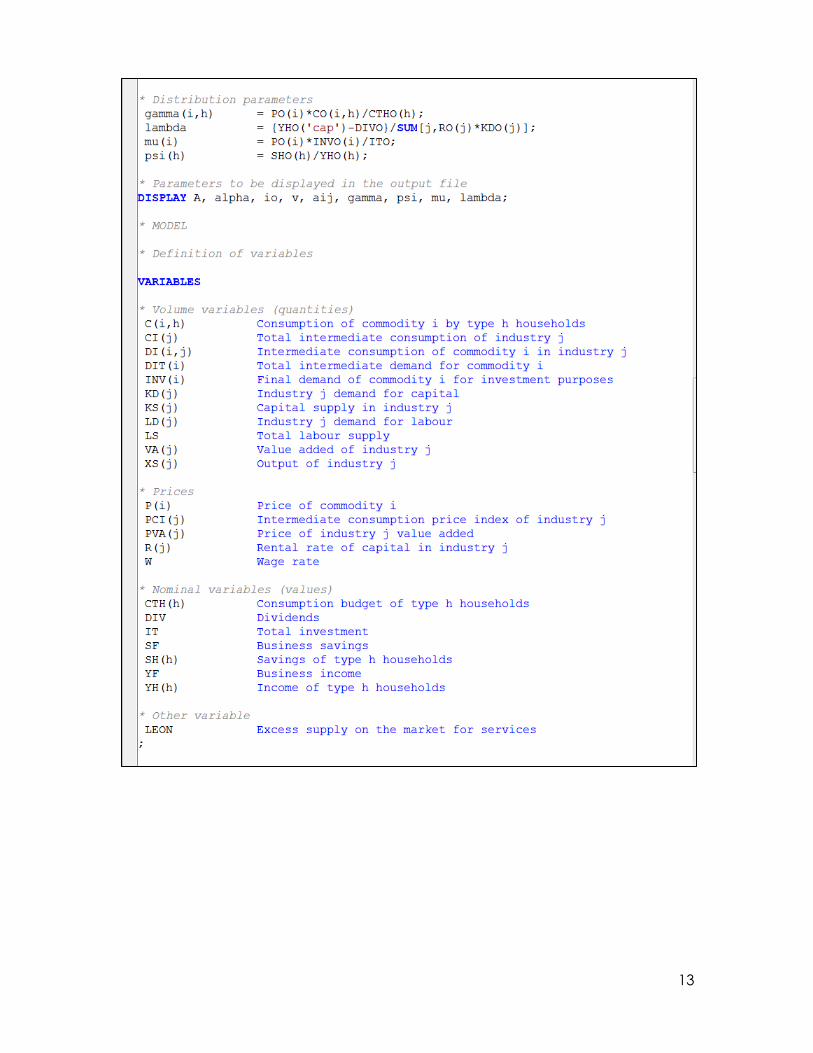
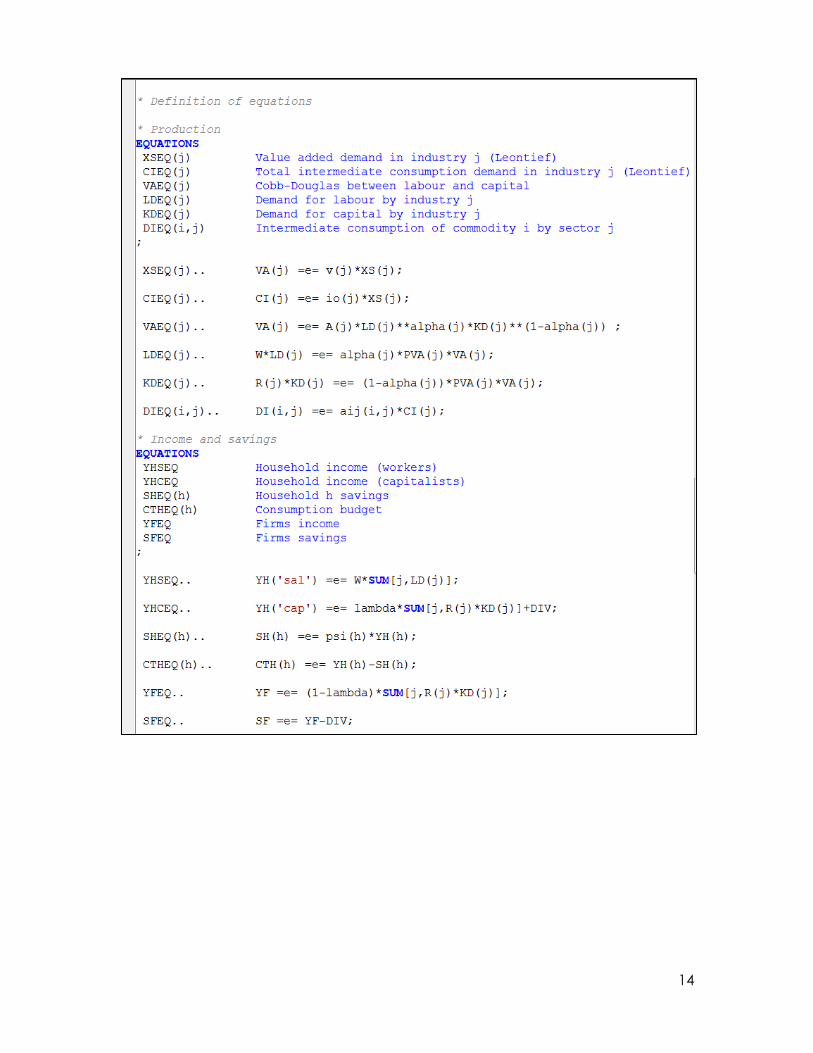
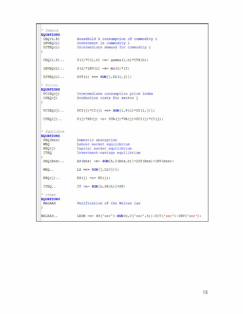
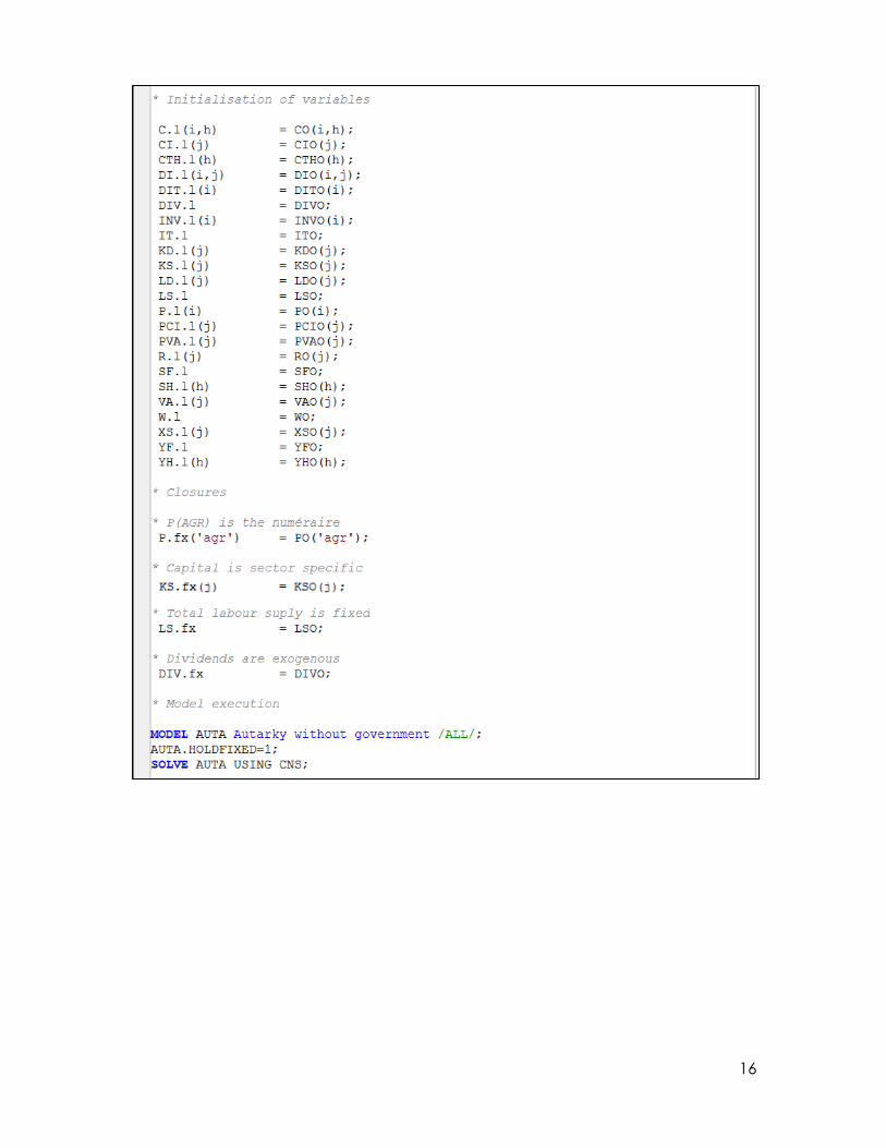
GAMS Code

11

12

13

14

15

16

17

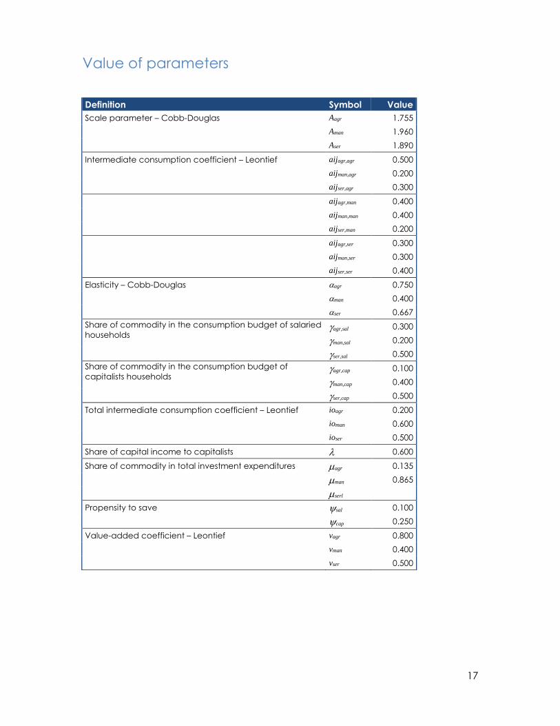
Value of parameters

Definition Symbol Value

Scale parameter – Cobb-Douglas Aagr 1.755

Aman 1.960

Aser 1.890

Intermediate consumption coefficient – Leontief aijagr,agr 0.500

aijman,agr 0.200

aijser,agr 0.300

aijagr,man 0.400

aijman,man 0.400

aijser,man 0.200

aijagr,ser 0.300

aijman,ser 0.300

aijser,ser 0.400

Elasticity – Cobb-Douglas agr 0.750

man 0.400

ser 0.667

Share of commodity in the consumption budget of salaried

households agr,sal 0.300

man,sal 0.200

ser,sal 0.500

Share of commodity in the consumption budget of

capitalists households agr,cap 0.100

man,cap 0.400

ser,cap 0.500

Total intermediate consumption coefficient – Leontief ioagr 0.200

ioman 0.600

ioser 0.500

Share of capital income to capitalists 0.600

Share of commodity in total investment expenditures agr 0.135

man 0.865

serl

Propensity to save sal 0.100

cap 0.250

Value-added coefficient – Leontief vagr 0.800

vman 0.400

vser 0.500

18

Simulations

SIM1: Impact of a 10% increase of capital supply in services

Definition Symbol Initial value Simulation Variation (%)

PRICES

• wage rate W 1 1.000 -0.019

Rental rate of capital

• agriculture Ragr 1 1.008 0.753

• manufacturing Rman 1 1.012 1.223

• services Rser 1 0.893 -10.726

Price of value added

• agriculture PVAagr 1 1.002 0.174

• manufacturing PVAman 1 1.007 0.724

• services PVAser 1 0.963 -3.723

Intermediate consumption pr ice index

• agriculture PCIagr 1 0.993 -0.694

• manufacturing PCIman 1 0.995 -0.459

• services PCIser 1 0.991 -0.925

Price of commodity

• agriculture

(numéraire) Pagr 1 1.000 -

• manufacturing Pman 1 1.000 0.014

• services Pser 1 0.977 -2.324

PRODUCTION AND FACTORS

Output

• agriculture XSagr 500 502.894 0.579

• manufacturing XSman 625 628.094 0.495

• services XSser 600 611.998 2.000

Value added

• agriculture VAagr 400 402.315 0.579

• manufacturing VAman 250 251.237 0.495

• services VAser 300 305.999 2.000

Labour

• agriculture LDagr 300 302.317 0.772

• manufacturing LDman 100 101.242 1.242

• services LDser 200 196.441 -1.780

• total LS 600 600 -

Capital

• agriculture KDagr 100 100.000 -

• manufacturing KDman 150 150.000 -

• services KDser 100 110.000 10.000

19

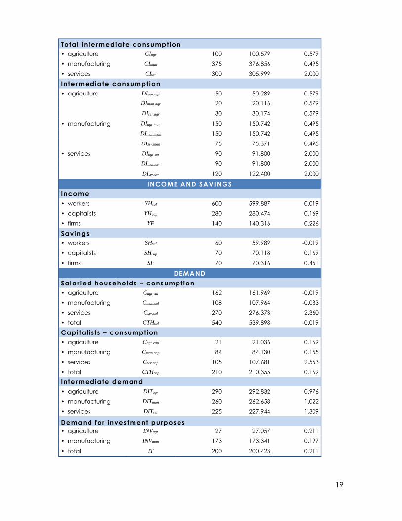
Total intermediate consumption

• agriculture CIagr 100 100.579 0.579

• manufacturing CIman 375 376.856 0.495

• services CIser 300 305.999 2.000

Intermediate consumption

• agriculture DIagr.agr 50 50.289 0.579

DIman.agr 20 20.116 0.579

DIser.agr 30 30.174 0.579

• manufacturing DIagr.man 150 150.742 0.495

DIman.man 150 150.742 0.495

DIser.man 75 75.371 0.495

• services DIagr.ser 90 91.800 2.000

DIman.ser 90 91.800 2.000

DIser.ser 120 122.400 2.000

INCOME AND SAVINGS

Income

• workers YHsal 600 599.887 -0.019

• capitalists YHcap 280 280.474 0.169

• firms YF 140 140.316 0.226

Savings

• workers SHsal 60 59.989 -0.019

• capitalists SHcap 70 70.118 0.169

• firms SF 70 70.316 0.451

DEMAND

Salar ied households – consumption

• agriculture Cagr.sal 162 161.969 -0.019

• manufacturing Cman.sal 108 107.964 -0.033

• services Cser.sal 270 276.373 2.360

• total CTHsal 540 539.898 -0.019

Capital ists – consumption

• agriculture Cagr.cap 21 21.036 0.169

• manufacturing Cman.cap 84 84.130 0.155

• services Cser.cap 105 107.681 2.553

• total CTHcap 210 210.355 0.169

Intermediate demand

• agriculture DITagr 290 292.832 0.976

• manufacturing DITman 260 262.658 1.022

• services DITser 225 227.944 1.309

Demand for investment purposes

• agriculture INVagr 27 27.057 0.211

• manufacturing INVman 173 173.341 0.197

• total IT 200 200.423 0.211

20

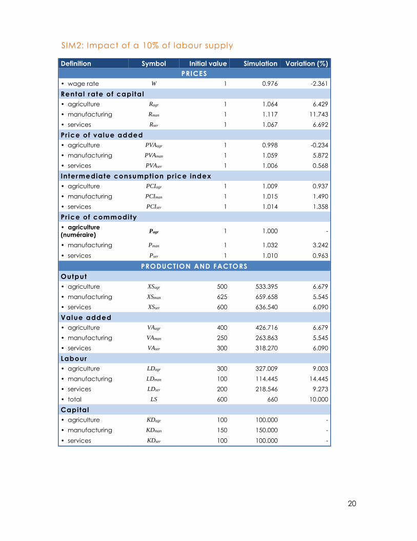
SIM2: Impact of a 10% of labour supply

Definition Symbol Initial value Simulation Variation (%)

PRICES

• wage rate W 1 0.976 -2.361

Rental rate of capital

• agriculture Ragr 1 1.064 6.429

• manufacturing Rman 1 1.117 11.743

• services Rser 1 1.067 6.692

Price of value added

• agriculture PVAagr 1 0.998 -0.234

• manufacturing PVAman 1 1.059 5.872

• services PVAser 1 1.006 0.568

Intermediate consumption pr ice index

• agriculture PCIagr 1 1.009 0.937

• manufacturing PCIman 1 1.015 1.490

• services PCIser 1 1.014 1.358

Price of commodity

• agriculture

(numéraire) Pagr 1 1.000 -

• manufacturing Pman 1 1.032 3.242

• services Pser 1 1.010 0.963

PRODUCTION AND FACTORS

Output

• agriculture XSagr 500 533.395 6.679

• manufacturing XSman 625 659.658 5.545

• services XSser 600 636.540 6.090

Value added

• agriculture VAagr 400 426.716 6.679

• manufacturing VAman 250 263.863 5.545

• services VAser 300 318.270 6.090

Labour

• agriculture LDagr 300 327.009 9.003

• manufacturing LDman 100 114.445 14.445

• services LDser 200 218.546 9.273

• total LS 600 660 10.000

Capital

• agriculture KDagr 100 100.000 -

• manufacturing KDman 150 150.000 -

• services KDser 100 100.000 -

21

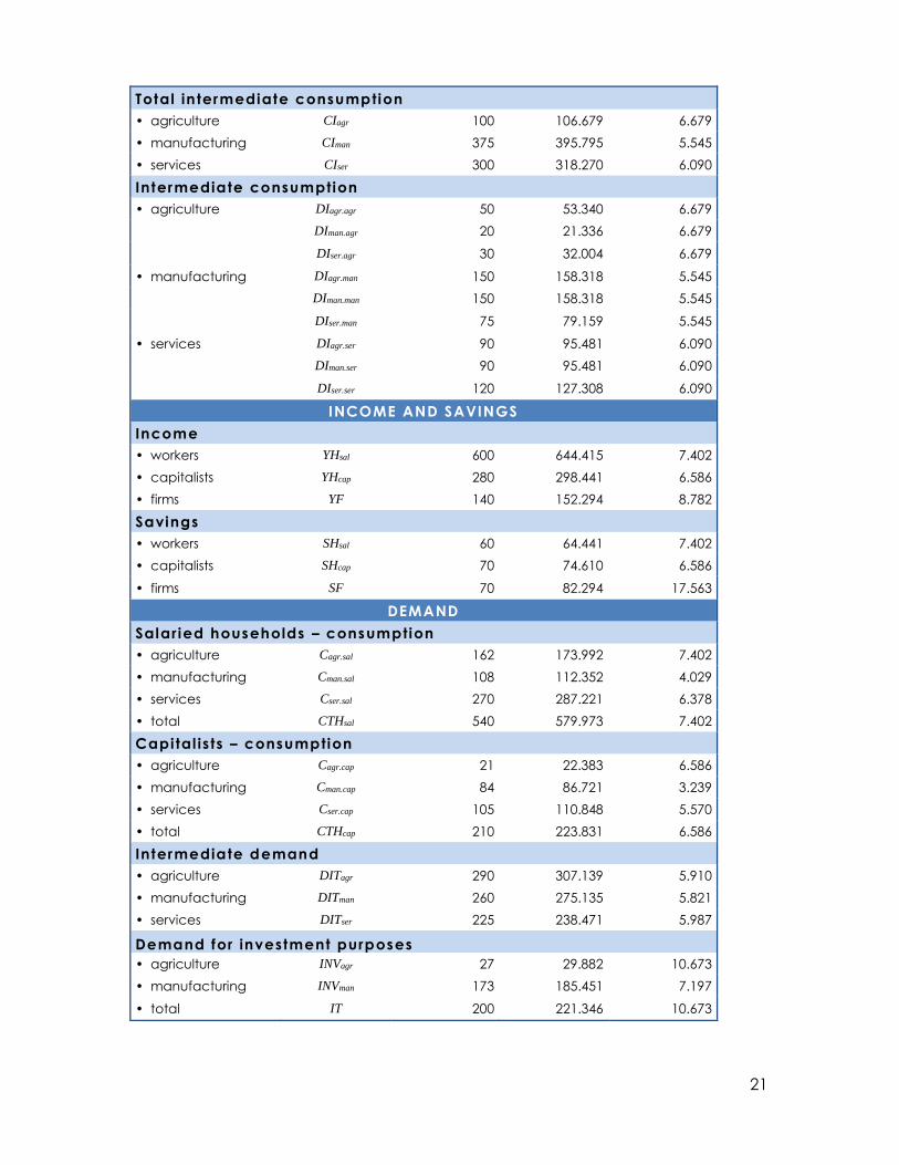
Total intermediate consumption

• agriculture CIagr 100 106.679 6.679

• manufacturing CIman 375 395.795 5.545

• services CIser 300 318.270 6.090

Intermediate consumption

• agriculture DIagr.agr 50 53.340 6.679

DIman.agr 20 21.336 6.679

DIser.agr 30 32.004 6.679

• manufacturing DIagr.man 150 158.318 5.545

DIman.man 150 158.318 5.545

DIser.man 75 79.159 5.545

• services DIagr.ser 90 95.481 6.090

DIman.ser 90 95.481 6.090

DIser.ser 120 127.308 6.090

INCOME AND SAVINGS

Income

• workers YHsal 600 644.415 7.402

• capitalists YHcap 280 298.441 6.586

• firms YF 140 152.294 8.782

Savings

• workers SHsal 60 64.441 7.402

• capitalists SHcap 70 74.610 6.586

• firms SF 70 82.294 17.563

DEMAND

Salar ied households – consumption

• agriculture Cagr.sal 162 173.992 7.402

• manufacturing Cman.sal 108 112.352 4.029

• services Cser.sal 270 287.221 6.378

• total CTHsal 540 579.973 7.402

Capital ists – consumption

• agriculture Cagr.cap 21 22.383 6.586

• manufacturing Cman.cap 84 86.721 3.239

• services Cser.cap 105 110.848 5.570

• total CTHcap 210 223.831 6.586

Intermediate demand

• agriculture DITagr 290 307.139 5.910

• manufacturing DITman 260 275.135 5.821

• services DITser 225 238.471 5.987

Demand for investment purposes

• agriculture INVagr 27 29.882 10.673

• manufacturing INVman 173 185.451 7.197

• total IT 200 221.346 10.673