Traffic Forecasting Manual Nevada Department of Transportation
122
Traffic Forecasting Manual Nevada Department of Transportation
Transcript of Traffic Forecasting Manual Nevada Department of Transportation

Traffic Forecasting Manual Nevada Department of Transportation

This page intentionally left blank

Traffic Forecasting Guidelines
August 2012
Nevada Department of Transportation

This page intentionally left blank

Acknowledgments
Traffic Forecasting Guidelines Nevada Department of Transportation i
These Traffic Forecasting Guidelines (Guidelines), document the Nevada Department of
Transportation’s (NDOT) techniques and accepted procedures for forecasting travel demand on
NDOT maintained roadways within the State of Nevada (State). These Guidelines are a
continuation of NDOT’s efforts to develop and publish an improved and consistent traffic
forecasting procedure.
These Guidelines have been developed using the Florida Department of Transportation (FDOT)
Project Traffic Forecasting Handbook as a model. However, procedures, examples, and
information specific to the State are included herein. These Guidelines outline the traffic
forecasting process, which has been part of the State’s forecasting procedures for several
years, into one document.
Contributors to these Guidelines include the following individuals.
Acevedo, Robert
Althoff, Judy
Bang, Peter
Bolgrien, Carl
Campbell, Don
Daniels, Seth
Dhanaraju, Sharan
Doenges, Dan
Erb, Jon
Foltz, Jeff
Geisler, Nancy
Greco, Tom
Hong, Hoang
Johnston, Jeremiah
Karachepone, John
Kazmi, Ali
Kramer, Brian
Krishnan, Shanthi
Lawson, Mike
Masterpool, Julie
McCurdy, Bryan
Morshed, Narges
Mudigonda, Anil
Mulazimoglu, Cigdem
Norberg, Keith
Primus, Chris
Ramirez, Joe
Rosenberg, Sondra
Sears, Kent
Solaegui, Paul
Thorsen, Scott
Travis, Randy
Wang, Xuan
Yellisetty, Vamshi

This page intentionally left blank
Table of Contents
Traffic Forecasting Guidelines Nevada Department of Transportation ii
1. Introduction and Overview ............................................................................. 1-1
1.1. Purpose and Objective of the Traffic Forecasting Guidelines ............................... 1-1
1.2. Chapter Overview ...................................................................................................... 1-1
1.3. Authority .................................................................................................................... 1-3
1.4. References ................................................................................................................. 1-3
1.5. Definitions .................................................................................................................. 1-5
1.6. Acronyms ................................................................................................................. 1-11
1.7. Guiding Principles and Standards when Preparing and Documenting Traffic
Forecasts ................................................................................................................. 1-12
1.7.1. Truth-in-data Principle .................................................................................... 1-12
1.7.2. Rounding Convention .................................................................................... 1-12
1.8. Traffic Forecasting Documentation and Deliverables........................................... 1-13
1.8.1. Methodology Memorandum ........................................................................... 1-13
1.8.2. Traffic Forecast Memorandum ....................................................................... 1-14
2. Traffic Forecasting for Different Types of Projects ...................................... 2-1
2.1. Common Types of Projects ...................................................................................... 2-1
2.2. Traffic Parameters and Chapter References by Project Type ................................ 2-2
2.2.1. Traffic Forecasting for Planning Projects .......................................................... 2-2
2.2.2. Traffic Forecasting for Environmental Analysis Projects ................................... 2-5
2.2.3. Traffic Forecasting for Design Projects ............................................................ 2-5
2.2.4. Traffic Forecasting for Operational Analysis Projects ....................................... 2-5
3. Traffic Data Sources and Factors .................................................................. 3-1
3.1. Traffic Data Collection Procedure ............................................................................ 3-1
3.2. Permanent Counts and Classification Counts ........................................................ 3-1
3.2.1. Automatic Traffic Recorders (ATRs)................................................................. 3-2
3.2.2. Automatic Vehicle Classification ...................................................................... 3-2
3.3. Short-Term Traffic Counts ........................................................................................ 3-2
3.4. Applying Traffic Adjustment Factors ....................................................................... 3-4
3.4.1. Seasonal Factor ............................................................................................... 3-4
3.4.2. Axle Factor....................................................................................................... 3-4
3.5. AADT, K30, D30, T% and PHF ...................................................................................... 3-4
3.5.1. Annual Average Daily Traffic (AADT) ............................................................... 3-4
3.5.2. K-Factor and K30 .............................................................................................. 3-5
3.5.3. D-Factor and D30 .............................................................................................. 3-5
3.5.4. Truck Percent (T%) .......................................................................................... 3-6
3.5.5. Peak Hour Factor (PHF) .................................................................................. 3-6
3.6. Locating and Using Data Sources ............................................................................ 3-8
3.6.1. NDOT’s Online Resources – TRINA and FTP Site ........................................... 3-8
3.6.2. Annual Traffic Reports ..................................................................................... 3-8

Table of Contents
Traffic Forecasting Guidelines Nevada Department of Transportation iii
3.6.3. Choosing a Data Source ................................................................................ 3-11
3.6.4. Identifying an ATR at a Location Similar to the Project Location .................... 3-13
3.7. Estimating AADT: Sample Case ............................................................................. 3-13
4. Traffic Forecasting Parameters, K30 & D30 ..................................................... 4-1
4.1. Definitions of K30 and D30 .......................................................................................... 4-1
4.2. Overview and Application of K30 .............................................................................. 4-3
4.3. Overview and Application of D30 .............................................................................. 4-4
4.4. Defining Demand Volume ......................................................................................... 4-6
4.5. Establishing Forecast Years ..................................................................................... 4-6
4.6. Determining Future Year K30 Values ........................................................................ 4-8
4.6.1. Adjusting K30 values ......................................................................................... 4-8
4.6.2. Acceptable K30 Values ..................................................................................... 4-9
4.7. Determining Future Year D30 Values ...................................................................... 4-11
4.7.1. Adjusting D30 values ....................................................................................... 4-11
4.7.2. Acceptable D30 Values ................................................................................... 4-12
4.8. Nonstandard K30 and D30 Values............................................................................. 4-14
4.9. Documenting Traffic Forecasts .............................................................................. 4-14
5. Traffic Forecasting with Travel Demand Models .......................................... 5-1
5.1. Overview of Travel Demand Models......................................................................... 5-1
5.2. Selecting a Travel Demand Model ............................................................................ 5-4
5.3. Reviewing the Accuracy of a Travel Demand Model ............................................... 5-4
5.3.1. Evaluating the Base Year Conditions ............................................................... 5-5
5.3.2. Refining the Base Year Travel Demand Model ................................................ 5-5
5.3.3. Determining the Necessity and Feasibility of Further Refinements ................... 5-6
5.3.4. Recommended Accuracy Levels (Consistency Thresholds) ............................. 5-7
5.4. Applying the Travel Demand Model for Future Year Conditions ......................... 5-14
5.4.1. Modifying Future Year Network and Land Use ............................................... 5-14
5.4.2. Evaluating Future Year Conditions ................................................................. 5-14
5.5. Executing the Travel Demand Model and Evaluating Outputs ............................. 5-14
5.5.1. Adjusting Travel Demand Model Output using NCHRP Report 255 Procedures (If
Necessary)..................................................................................................... 5-15
5.5.2. Converting Travel Demand Model Output ...................................................... 5-18
5.5.3. Comparison of Model Forecasts with Historical Trend Projection Results ...... 5-20
5.6. Obtaining Design Year AADT from the Travel Demand Model’s Future Year AADT
Estimates ................................................................................................................. 5-21
5.7. Documenting Traffic Forecasts .............................................................................. 5-23
6. Traffic Forecasting without a Travel Demand Model .................................... 6-1
6.1. Overview of Historical Trend Projection Analyses ................................................. 6-1

Table of Contents
Traffic Forecasting Guidelines Nevada Department of Transportation iv
6.2. Procedures for Performing Historical Trend Projection Analyses......................... 6-1
6.2.1. Assembling the Data ........................................................................................ 6-2
6.2.2. Establishing Traffic Growth Trends .................................................................. 6-2
6.2.3. Developing Preliminary Traffic Projection ......................................................... 6-3
6.2.4. Verifying Traffic Forecasts for Reasonableness ............................................... 6-4
6.2.5. Developing Traffic Forecast in Detail................................................................ 6-4
6.2.6. Preparing for Final Review and Documentation ............................................... 6-5
6.3. Other Available Resources for Forecasting Traffic in an Area without a Travel
Demand Model ........................................................................................................... 6-5
6.4. Historical Trend Projection Analysis: Sample Case ............................................... 6-6
7. Directional Design Hourly Volume Estimates ............................................... 7-1
7.1. Developing Directional Design Hour Traffic Volumes ............................................ 7-1
7.2. LOS Operational Analysis Guidelines ...................................................................... 7-2
7.3. Definition of a Constrained Roadway ...................................................................... 7-2
7.4. Determining Peak Hour Design Volumes from DDHV ............................................. 7-4
7.5. Determining Peak Hour Design Volume: Sample Case .......................................... 7-5
7.6. Documenting Traffic Forecasts ................................................................................ 7-6
8. Estimating Intersection Turning Movements ................................................ 8-1
8.1. Estimating Intersection Turning Movements .......................................................... 8-1
8.2. TurnsW32 ................................................................................................................... 8-2
8.2.1. TurnsW32 Methodology ................................................................................... 8-2
8.2.2. TurnsW32 Program Interface ........................................................................... 8-3
8.3. Other Tools/Techniques ............................................................................................ 8-8
8.3.1. TURNS5-V02 ................................................................................................... 8-9
8.3.2. TMTOOL .......................................................................................................... 8-9
8.3.3. Manual Method ................................................................................................ 8-9
8.3.4. Growth Factor Technique ............................................................................... 8-10
8.3.5. Methods from the NCHRP Report 255 ........................................................... 8-10
8.4. Summary .................................................................................................................. 8-11
9. Truck Traffic Forecasting................................................................................ 9-1
9.1. Truck Traffic Forecasting Methodology ................................................................... 9-1
9.2. Truck Traffic Forecasting Procedures ..................................................................... 9-3
9.2.1. Truck Traffic Forecasting if Historical Truck AADT Data is Available for the
Project Location ............................................................................................... 9-3
9.2.2. Truck Traffic Forecasting if Historical Data is Not Available for the Project
Location ........................................................................................................... 9-4
9.2.3. Truck Traffic Forecasting if Historical Data is Not Available and a Location with
Similar Characteristics Cannot Be Identified .................................................... 9-4

Table of Contents
Traffic Forecasting Guidelines Nevada Department of Transportation v
9.2.4. Truck Traffic Forecasting if No Suitable Truck AADT Data is Available ............ 9-4
9.3. Estimating Truck Percent (T%) ................................................................................. 9-5
9.4. Peak Hour Truck Volumes and Peak Hour Truck Percent ...................................... 9-5
9.5. Documenting Truck Traffic Forecast ....................................................................... 9-6
Appendix A..................................................................................................................A-1
Appendix B..................................................................................................................B-1

List of Figures
Traffic Forecasting Guidelines Nevada Department of Transportation vi
Figure 2-1 Contrasting Characteristics of the Different Types of Projects ................................ 2-2
Figure 3-1 FHWA Classification Scheme “F” ........................................................................... 3-3
Figure 3-2 Traffic Factors ........................................................................................................ 3-7
Figure 3-3 Example Hourly Traffic Report from Short-Term Count Station #030268 ............... 3-9
Figure 3-4 Obtaining Base Year Traffic Parameters from Relevant Data Sources ................. 3-12
Figure 3-5 Example ATR Summary Statistics ....................................................................... 3-14
Figure 4-1 Estimating the Future Year Traffic Forecasting Parameters ................................... 4-2
Figure 4-2 Relation between Peak-Hour and AADT Volume ................................................... 4-4
Figure 4-3 Traffic Volume Directional Distribution ................................................................... 4-5
Figure 5-1 Traffic Forecasting with Travel Demand Models..................................................... 5-3
Figure 5-2 Sample Year 2008 Travel Demand Model Output Plot ......................................... 5-11
Figure 6-1 Establishing Growth Trend and Developing Preliminary Traffic Projection ............. 6-3
Figure 6-2 Traffic Growth Trend .............................................................................................. 6-8
Figure 7-1 Constrained Roadway LOS Example Illustrating LOS Breakdown Year ................. 7-4
Figure 8-1 Manual Data Entry and the Furness Screen ........................................................... 8-5
Figure 8-2 Furness Screen and Iteration Settings ................................................................... 8-6
Figure 8-3 Results Screen ...................................................................................................... 8-7
Figure 9-1 Truck Traffic Forecasting ....................................................................................... 9-2

List of Tables
Traffic Forecasting Guidelines Nevada Department of Transportation vii
Table 1-1 Rounding Convention - Calculation of AADT ......................................................... 1-12
Table 1-2 Traffic Forecasting Guidelines Checklist ............................................................... 1-15
Table 2-1 Traffic Parameters for the Different Types of Projects ............................................. 2-3
Table 3-1 Application of Daily Factors to Raw Counts ........................................................... 3-15
Table 4-1 Suggested Peak Hour factors for Future Years Analysis ......................................... 4-6
Table 4-2 Establishing Forecast Years .................................................................................... 4-7
Table 4-3 Recommended K30 values for Traffic Forecasting ................................................. 4-10
Table 4-4 Recommended D30 values for Traffic Forecasting ................................................. 4-13
Table 5-1 Consistency Thresholds: Percent Deviation Thresholds for every Link across Cutlines
and all Project Corridor Links .................................................................................. 5-9
Table 5-2 Consistency Thresholds: CV(RMSE) Thresholds for every Link across Cutlines and
all Project Corridor Links ......................................................................................... 5-9
Table 5-3 Sample Percent Deviation Comparison along all Project Corridor Links ................ 5-12
Table 5-4 Sample CV(RMSE) Comparison along all Project Corridor Links .......................... 5-13
Table 5-5 Sample NCHRP Report 255 Adjustments to the Travel Demand Model Output .... 5-17
Table 5-6 Sample Calculation of MOCF ................................................................................ 5-19
Table 6-1 Historical AADT for Use in Trend Projection ............................................................ 6-7
Table 7-1 Existing Peak Hour Directional Volumes ................................................................. 7-5

Chapter 1 Introduction and Overview
Traffic Forecasting Guidelines Nevada Department of Transportation 1-1
1. Introduction and Overview
This chapter provides a general introduction and overview of the Traffic Forecasting Guidelines
(Guidelines). This chapter discusses:
The purpose and objectives of these Guidelines;
A general overview of the nine chapters included in these Guidelines;
The authority, references, definitions, and acronyms that are used throughout these
Guidelines;
The guiding principles that are relevant in creating and preparing traffic forecasts;
and
The deliverables necessary to complete the traffic forecasting process.
In addition, the Guidelines note useful references throughout to assist the analyst with the traffic
forecasting process.
1.1. Purpose and Objective of the Traffic Forecasting Guidelines
The purpose of these Guidelines is to document the Nevada Department of Transportation’s
(NDOT) techniques and accepted procedures for forecasting travel demand on NDOT
maintained roadways within the State of Nevada (State). Traffic forecasts are ultimately used to
determine the number of lanes a corridor or project may require. The objective of the Guidelines
is to facilitate the creation and evaluation of traffic forecasts that are reproducible and
defendable, resulting in consistent and sound forecasts and analyses on all applicable
transportation projects. The intended audience for these Guidelines are practitioners who
develop traffic forecasts for state highways in Nevada. These Guidelines are written to eliminate
conflicts and provide consistency in accepting and approving technical methodologies for traffic
forecasts, which in turn lead to time and cost savings for applicants, consultants, travel demand
model users, and NDOT.
In all, the Guidelines identify the traffic parameters necessary for accurate traffic forecasting
across various types of transportation projects. The Guidelines also offer direction for producing
traffic forecasts for planning projects, environmental analyses/studies, design projects, and
operational studies/projects. Also presented is the method on how to use the outputs from travel
demand models to produce traffic forecasts and how to implement historical trend projection
analysis techniques for producing traffic forecasts when a travel demand model is not available
for the project location.
1.2. Chapter Overview
These Guidelines consist of nine chapters, and a brief overview of each chapter is provided
below.

Chapter 1: Introduction and Overview
Traffic Forecasting Guidelines Nevada Department of Transportation 1-2
Chapter One: Introduction and Overview
In part, this chapter describes an overall purpose and objective of these Guidelines, all current
and applicable references, and the definitions used in the traffic forecasting process. The truth-
in-data principle (requirements for reporting sources and uncertainties in forecast) and the
rounding convention (American Association of State Highway and Transportation Officials
[AASHTO] rounding convention to reflect uncertainty of estimates and forecasts) are both
explained in this chapter.
Chapter Two: Traffic Forecasting for Different Types of Projects
This chapter refers the analyst to appropriate sections within the Guidelines that relate to
specific project requirements. The chapter also addresses traffic forecasting requirements for
planning projects, environmental analysis projects, design projects, and operational analysis
projects, all the while directing the analyst to the appropriate Guidelines chapter for
methodology descriptions.
Chapter Three: Traffic Data Sources and Factors
This chapter describes the traffic data sources and factors used in forecasting traffic, which are
Seasonal Factors, Axle Factors, Annual Average Daily Traffic (AADT) volumes, the Design Hour
Factor (K30), the Directional Distribution Factor (D30), and Truck Percent (T%). The chapter also
speaks to the connection between these traffic factors and NDOT’s sources for these factors.
The relationship among Average Daily Traffic (ADT), the various traffic factors and AADT, and
the procedure to estimate AADT volumes from ADT volumes is also explained with appropriate
examples.
Chapter Four: Traffic Forecasting Parameters, K30 & D30
This chapter describes the process of estimating K30 and D30 for future years. The chapter also
discusses the acceptable value ranges of K30 and D30 by roadway functional classification. An
example of estimating K30 and D30 for future years is provided alongside NDOT’s policy for
establishing forecast years and guidance on the time periods and years for which forecasts are
to be developed.
Chapter Five: Traffic Forecasting with Travel Demand Models
This chapter presents a description of the appropriate methods and procedures for forecasting
future corridor or project traffic in areas that have a travel demand model. The chapter explains
the use of travel demand model outputs for traffic forecasting. Methods for using travel demand
model outputs, analysis of travel demand model results, refinements to base year travel
demand models, comparison of travel demand model performance, and reasonableness checks
for future years in the traffic forecasting process are discussed therein. The chapter also
provides acceptable accuracy levels for corridor and project specific use.

Chapter 1: Introduction and Overview
Traffic Forecasting Guidelines Nevada Department of Transportation 1-3
Chapter Six: Traffic Forecasting without a Travel Demand Model
This chapter describes the appropriate methods of performing historical trend projection
analysis. Relevance of growth rates from historical traffic counts as well as examination of local
land use plans, population forecasts, and other indicators of future growth in the traffic
forecasting process are also included in the chapter.
Chapter Seven: Directional Design Hourly Volume Estimates
This chapter defines the appropriate method for the calculation of Directional Design Hourly
Volumes (DDHV) from AADT volumes. DDHV is the basic traffic projection to be used in State
roadway projects that require traffic forecasts.
Chapter Eight: Estimating Intersection Turning Movements
This chapter explains the popular methods and tools available for balancing and estimating
turning movement volumes at intersections. Many of these tools use the techniques outlined in
National Cooperative Highway Research Program (NCHRP) Report 255 and other iterative
methods. The chapter includes a thorough overview of the preferred tool (TurnsW32) for use
when estimating turning movements as well as the other techniques and tools that are
acceptable for use in the State.
Chapter Nine: Truck Traffic Estimation
This chapter describes the guidelines and techniques for forecasting truck volumes.
Appendices
Appendix A offers guidance for identifying Automatic Traffic Recorders (ATRs) at locations with
characteristics similar to that of the project location. Appendix B offers a simple calculation
technique for obtaining balanced turning movement volumes from approach volumes at three-
legged and four-legged intersections.
1.3. Authority
The following policies and statutes establish the authority upon which these Guidelines are
structured.
Process for Requesting, Developing and Approving Traffic Data Used on NDOT
Projects, NDOT Policy # 03-03
NDOT’s Transportation Policy (TP)
Nevada Revised Statutes (NRS) 277, 277A, 278, 278A, 408, 410, 481A, and 540A
1.4. References
The following references provide insight to assist the analyst with the traffic forecasting process.
AASHTO. 2011. A Policy on Geometric Design of Highways and Streets. 6th Edition.

Chapter 1: Introduction and Overview
Traffic Forecasting Guidelines Nevada Department of Transportation 1-4
Dowling Associates, Inc. 2002. TurnsW32: Technical Documentation.
Federal Highway Administration (FHWA). 2010. Interim Guidance on the Application of
Travel and Land Use Forecasting in NEPA.
FHWA. 2010. Model Validation and Reasonableness Checking Manual. Travel Model
Improvement Program.
Florida Department of Transportation (FDOT). 2002. Project Traffic Forecasting
Handbook. October.
FDOT. 2012. Project Traffic Forecasting Handbook. January.
Hauer et al. 1983. “The Accuracy of Estimation of Turning Flows from Automatic
Counts,” Traffic Engineering and Control, Vol. 24, No. 1.
Institute of Transportation Engineers (ITE). 2008. Trip Generation Manual. 8th Edition.
NCHRP. 1982. Highway Traffic Data for Urbanized Area Project Planning and Design.
Report 255.
NCHRP. 1998. Travel Estimation Techniques for Urban Planning. Report 365.
NDOT. 2011. Traffic Monitoring System (TMS).
NDOT. 2012. Traffic Information FTP Site. <ftp://ftp.nevadadot.com/traffic information/>.
NDOT. 2012. Annual Traffic Report. <http://www.nevadadot.com/About_NDOT/NDOT_
Divisions/Planning/Traffic/Annual_Traffic_Reports.aspx>.
NDOT. 2012. Traffic Records Information Access (TRINA). <http://apps.nevada
dot.com/Trina/>.
NDOT. 2010. Vehicle Classification Distribution Report.
NDOT. 2010. Road Design Guide.
Nevada State Demographer’s Office. 2010. Nevada County Population Projections 2010
to 2030. <http://nvdemography.org/wp-content/uploads/2011/09/2011-Projections
-Email-attachment-090911.pdf>.
Ohio Department of Transportation. 2007. Ohio Certified Traffic Manual. June.
Oregon Department of Transportation. 2006. Analysis Procedures Manual. April.
Schaefer, Mark C. 1988. “Estimation of Intersection Turning Movements from Approach
Counts.” Institute of Transportation Engineers (ITE) Journal. October 1988.

Chapter 1: Introduction and Overview
Traffic Forecasting Guidelines Nevada Department of Transportation 1-5
Stone, J.R., Han Y., and Ramkumar, R. 2006. North Carolina Forecasts for Truck Traffic.
July.
Texas Department of Transportation. 2001. Traffic Data and Analysis Manual.
September.
Transportation Research Board. 1981. Estimation of Turning Flows from Automatic
Counts. Record No. 795.
Transportation Research Board. 2010. Highway Capacity Manual (HCM).
Virginia Department of Transportation. 2009. Virginia Transportation Modeling (VTM)
Policies and Procedures Manual. May.
Zuylen, H. J. Van. 1979. “The Estimation of Turning Flows on a Junction,” Traffic
Engineering Control, Vol. 20, No. 12.
1.5. Definitions
The following are the definitions of terms used throughout these Guidelines. Many of these
terms are referenced from the Highway Capacity Manual (HCM 2010), A Policy on Geometric
Design of Highways and Streets (AASHTO), and the Process for Requesting, Developing, and
Approving Traffic Data Used on NDOT Projects (NDOT Policy # 03-03).
Annual Average Daily Traffic (AADT): The total volume of traffic on a roadway
segment for one year, divided by the number of days in the year. This volume is usually
estimated by adjusting a short-term traffic count with seasonal factors.
Annual Average Day of Week (AADW): The estimate of traffic volume for each day of
the week, over the period of one year. It is calculated from ATR data as the sum of all
traffic for each day of the week during a year, divided by the occurrences of that day
during the year.
Annual Average Weekday Traffic (AAWDT): The estimate of typical traffic during a
weekday (usually defined as Monday through Friday) calculated from data measured at
ATRs. If AAWDT was not estimated based on traffic during the weekdays defined above,
the weekdays that were the basis for the AAWDT estimate are to be specified. (e.g.,
Monday through Thursday).
Adjusted Count: An estimate of a traffic statistic calculated from a base traffic count
that has been adjusted by application of axle, seasonal, or other defined factors
(AASHTO).
Average Daily Traffic (ADT): The total traffic volume during a given time period (more
than a day and less than a year), divided by the number of days in that time period. The

Chapter 1: Introduction and Overview
Traffic Forecasting Guidelines Nevada Department of Transportation 1-6
days that were the basis for the ADT measurement are to be specified. (e.g., Tuesday,
Wednesday).
Average Weekday Traffic (AWDT): The total volume of traffic on a roadway segment
during the weekdays (Monday through Thursday) and during a given time period (less
than a year), divided by the number of weekdays in that period. If AWDT was not
estimated based on traffic during the weekdays defined above, the weekdays that were
the basis for the AWDT estimate are to be specified. (e.g., Monday through Thursday).
Axle Factor: The factor developed to adjust vehicle axle sensor base data for the
incidence of vehicles with more than two axles. Axle Factor is the estimate of total axles
based on automatic vehicle classification data, divided by the total number of vehicles
counted.
Base Count: A traffic count that has not been adjusted with Axle Factors (effects of
trucks) or for seasonal (day of the week/month of the year) effects (AASHTO).
Base Data: The unedited and unadjusted measurements of traffic volume, vehicle
classification, and vehicle or axle weight (AASHTO).
Base Year: The initial year of the forecast period; base year is the year from which
projections are made. The base year could be the same as or different from the model
calibration year. For example, the model calibration year could be 2008, the year from
which planning variables data are input for calibration. However, the base year for
forecasts could be 2011, the year for which the model traffic volumes were validated.
Typically, the base year is as close as possible to the existing year.
Calibration (Model): An extensive analysis of a travel demand model based on census,
survey, traffic count, and other information.
Capacity: The maximum sustainable hourly flow rate at which persons or vehicles
reasonably can be expected to traverse a point or a uniform section of a lane or roadway
during a given time period under prevailing roadway, environmental, traffic, and control
conditions (HCM 2010).
Count: The data collected as a result of measuring and recording traffic characteristics,
such as vehicle volume, classification, speed, weight, or a combination of these
characteristics (AASHTO).
Counter: Any person or device that collects traffic characteristics data.
Current Traffic Data: Traffic data as it is estimated to exist today (NDOT Policy # 03-
03).

Chapter 1: Introduction and Overview
Traffic Forecasting Guidelines Nevada Department of Transportation 1-7
Cutline: Similar to a screenline; however, a cutline is shorter and crosses corridors
rather than regional flows. Cutlines should be established to intercept travel along only
one axis.
Daily Truck Volume: The total volume of trucks on a roadway segment in a day.
Demand Volume: The traffic volume expected to desire service past a point or segment
of a roadway at some future time, or the traffic currently arriving or desiring service past
such a point, usually expressed as vehicles per hour (vph).
Design Hour: An hour with a traffic volume that represents a reasonable value for
designing the geometric and control elements of a roadway. Design hour is usually the
30th highest hour of the design year.
Design Hour Volume (DHV): The traffic volume expected to use a roadway segment
during the 30th highest hour of the design year. The DHV is related to AADT by the K-
factor.
Design Period: The number of years from the initial application of traffic until the first
planned major resurfacing or overlay (AASHTO).
Design Year: The year for which the roadway is designed. This is usually 20 years from
the opening year but may be any time within a range of years from the present (for
restoration type projects) to 20 or more years in the future (for new construction type
projects).
Directional Design Hour Volume (DDHV): The traffic volume expected to use a
roadway segment during the 30th highest hour of the design year in the peak direction.
D-Factor: The percentage of total, two-way peak hour traffic that occurs in the peak
direction. D-factor is also known as Directional Distribution.
D30: The proportion of traffic in the 30th highest hour of the design year traveling in the
peak direction.
Existing Year: The latest year for which field traffic data is available.
Factor: A number that represents a ratio of one number to another number. The factors
used in these Guidelines are K-factor, D-factor, Peak Hour Factor (PHF), Seasonal
Factor, and Axle Factor.
Forecast Period: The total length of time covered by the traffic forecast. It is equal to
the period from the base year to the design year. For existing roads, the forecast period
will extend from the year in which the forecast is made and, therefore, must include the
period prior to the project being completed as well as the life of the project improvement.

Chapter 1: Introduction and Overview
Traffic Forecasting Guidelines Nevada Department of Transportation 1-8
Future Traffic Data: Traffic data that must be forecasted (NDOT Policy # 03-03).
Future Year: Any year that is later than the base year.
Historical Traffic Data: Traffic data from a time period before today (NDOT Policy # 03-
03).
Horizon Years: Horizon years of the Regional Transportation Plan (RTP) are the years
identified as those used for air quality modeling and project funding. Horizon years
include the final year of the RTP and interim years. The interim years must begin “no
more than 10 years from the base year used to validate the transportation demand
planning model,” be no more than 10 years apart, and end no later than the plan.
Interim Year: Interim year can be any year between the opening year and the design
year of a project. It is usually 10 years into the future from the opening year of a project
and 10 years prior to the design year of the project.
K-Factor: The ratio of the traffic volume in the study hour to the AADT.
K30: The proportion of AADT occurring during the 30th highest hour of the design year.
K30 is also commonly known as the Design Hour Factor.
Level of Service (LOS): A quantitative stratification of a performance measure or
measures that represent quality of service. LOS is measured on an A to F scale, with
LOS A representing the best operating conditions from the traveler’s perspective and
LOS F the worst (HCM 2010).
Long Range Plan: A document with a 20-year planning horizon required of each MPO
that forms the basis for an annual transportation improvement program (TIP). A long
range plan is developed pursuant to Title 23 United States Code 134 and Title 23 Code
of Federal Regulations Part 450 Subpart C. The long range plan is also known as the
RTP.
Model Calibration Year: The year the travel demand model was calibrated for, and the
year the planning variables (land use, population, etc.) were based upon.
Model Output Conversion Factor (MOCF): The MOCF is used to convert the traffic
volumes (if other than AADT) generated by a travel demand model to AADT.
Monthly Average Daily Traffic (MADT): The estimate of mean traffic volume for a
month, calculated by the sum of Monthly Average Days of the Week (MADWs) divided
by seven; or in the absence of a MADW for each day of the week, divided by the number
of available MADWs during the month (AASHTO).

Chapter 1: Introduction and Overview
Traffic Forecasting Guidelines Nevada Department of Transportation 1-9
Monthly Average Days of the Week (MADW): The estimate of traffic volume for each
day of the week over the period of one month. MADW is calculated from ATR data as
the sum of all traffic for each day of the week during a month, divided by the occurrences
of that day during the month.
Monthly Average Weekday Traffic (MAWDT): The estimate of traffic volume for
weekdays (defined as Monday through Thursday in the State) over the period of a given
month. It is calculated from ATR data as the sum of all traffic for weekdays (Monday
through Thursday in the State) of the month, divided by the number of occurrences of
weekdays during the same month.
Monthly Average Weekend Traffic (MAWET): The estimate of traffic volume for the
weekends (Saturday and Sunday) over the period of a given month. It is calculated from
ATR data as the sum of all traffic for the weekends (Saturday and Sunday) during a
month, divided by the number of occurrences of weekend days during the same month.
Monthly Seasonal Factor: A seasonal adjustment factor derived by dividing the AADT
by the MADT.
Opening Year: The year in which a given roadway will be opened/available for use by
the public.
Peak Hour Factor (PHF): The hourly volume during the analysis hour divided by the
peak 15-minute flow rate within the analysis hour. The PHF is also considered a
measure of traffic demand fluctuation within the analysis hour (HCM 2010).
Peak Hour-Peak Direction: The direction of travel (during the 60-minute peak hour) that
contains the highest percentage of travel.
Peak-to-Daily Ratio: The highest hourly volume of a day divided by the daily volume.
Permanent Count: A traffic count continuously recorded at an ATR.
Regional Transportation Plan (RTP): An RTP is an urbanized region’s long-term plan
for its transportation system. An RTP serves as a region’s master plan for guiding future
transportation investments and often has a time horizon of 20 to 30 years into the future.
An RTP may also be referred to as a region’s long range transportation plan, and it is
prepared and adopted by a region’s MPO (see long range plan). An RTP is based on
projections of growth and economic activity and the resulting need for improvements to
transportation infrastructure. An RTP is required by State and federal law for MPOs
designated in urbanized areas with a population greater than 50,000.
Screenline: An imaginary line that intercepts major traffic flows through a region. A
screenline is usually along a physical barrier, such as a river or railroad tracks, and splits

Chapter 1: Introduction and Overview
Traffic Forecasting Guidelines Nevada Department of Transportation 1-10
a study area into parts. Traffic counts and possibly interviews are conducted along this
line as a means to compare simulated travel demand model results to field results as
part of the calibration/validation of a travel demand model.
Seasonal Factor: Parameters used to adjust base counts that consider travel behavior
fluctuations by day of the week and month of the year.
Service Flow Rate: The maximum directional rate of flow that can be sustained in a
given segment under prevailing roadway, traffic, and control conditions without violating
the criteria for a given LOS standard (HCM 2010).
Standard Deviation: A measure of the dispersion of a set of data from its mean.
TP-D: The proportion of daily truck traffic occurring in the peak hour of truck traffic. TP-D is
the ratio of peak hour truck volume to the daily truck volume.
Traffic Analysis Zone (TAZ): The basic unit of analysis representing the spatial
aggregation of people within an urbanized area. A TAZ may have a series of zonal
characteristics associated with it that are used to explain travel flows among zones.
Typical characteristics include the number of households and the number of people that
work and/or live in a particular area.
Traffic Data: Any measure of movement by persons or vehicles (NDOT Policy # 03-03).
Truck Percent (T%): The proportion of the number of trucks on a roadway to the total
number of vehicles on the roadway, expressed as a percentage.
Validation: An analysis of a travel demand model based on traffic count and other
information. A validation is usually less extensive than a calibration.
Vehicle Hours of Travel (VHT): A statistic describing the amount of vehicular travel
time in a given area. It is calculated by multiplying the total number of vehicles with the
total number of hours that vehicles travel. The VHT is most commonly used to compare
alternative transportation systems in a planning context. In general, if alternative “A”
reflects a VHT of 150,000 and alternative “B” reflects a VHT of 200,000, it can be
concluded that alternative “A” is better in that drivers are getting to their destinations
quicker.
Vehicle Miles of Travel (VMT): A statistic describing the amount of vehicular travel in a
given area. It is calculated by multiplying the total number of vehicles with the total
number of miles that are traversed by those vehicles.
Volume to Capacity Ratio (v/c): Either the ratio of demand volume to capacity or the
ratio of service flow volume to capacity, depending on the particular situation.

Chapter 1: Introduction and Overview
Traffic Forecasting Guidelines Nevada Department of Transportation 1-11
1.6. Acronyms
The following is a list of the acronyms that are used throughout these Guidelines.
ADT Average Daily Traffic
AADT Annual Average Daily Traffic
AADW Annual Average Day of Week
AASHTO American Association of State Highway and Transportation Officials
AAWDT Annual Average Weekday Traffic
ADT Average Daily Traffic
ATR Automatic Traffic Recorder
AWDT Average Weekday Traffic
D-Factor Proportion of traffic in the peak direction
D30 Proportion of traffic in the peak direction for the 30th highest hour
DAF Day Factor
DHV Design Hour Volume
DDHV Directional Design Hour Volume
FHWA Federal Highway Administration
FTP File Transfer Protocol
HCM Highway Capacity Manual
K-Factor Ratio of DHV to AADT
K30 Ratio of DHV to AADT for the 30th highest hour
LGCP Local Government Comprehensive Plan
LOS Level of Service
MADT Monthly Average Daily Traffic
MADW Monthly Average Day of Week
MAWDT Monthly Average Weekday Traffic (Weekdays considered: Monday to
Thursday)
MAWET Monthly Average Weekend Traffic
MOCF Model Output Conversion Factor
MPO Metropolitan Planning Organization
NCHRP National Cooperative Highway Research Program
NDOT Nevada Department of Transportation
NEPA National Environmental Policy Act
PHF Peak Hour Factor
RTP Regional Transportation Plan
TAZ Traffic Analysis Zone
TMS Traffic Monitoring System
TRINA Traffic Records Information Access
v/c Volume to Capacity Ratio
VHT Vehicle Hours of Travel

Chapter 1: Introduction and Overview
Traffic Forecasting Guidelines Nevada Department of Transportation 1-12
VMT Vehicle Miles of Travel
vph Vehicles Per Hour
1.7. Guiding Principles and Standards when Preparing and
Documenting Traffic Forecasts
The truth-in-data principle and the rounding convention are both to be applied when preparing
and documenting traffic forecasts.
1.7.1. Truth-in-data Principle
The controlling truth-in-data principle for creating traffic forecasts is to express the sources and
uncertainties of the forecast. The goal of the principle is to provide the person reviewing the
forecast with the information needed to make appropriate choices regarding the applicability of
the forecast for particular purposes. For the analyst (the developer of the traffic forecast), it
means clearly stating the input assumptions and their sources, defining known uncertainties,
and providing the forecast in a form that a reviewer can understand and use.
1.7.2. Rounding Convention
To reflect the uncertainty of estimates and forecasts, volumes are to be reported according to
the following rounding convention. Table 1-1 specifies the rounding convention relevant to the
calculation of AADT; this rounding convention was adapted from AASHTO standards.
Table 1-1 Rounding Convention - Calculation of AADT
Forecast Volume Round to Nearest
<100 10
100 to 999 50
1,000 to 9,999 100
10,000 to 99,999 500
>99,999 1,000
In the case of the calculation of DDHV, greater precision is usually required, and therefore, the
estimates are to be rounded to the nearest 10. The analyst is to use five as the minimum value
for a projected turning movement volume.
These recommendations apply only to reported values. The unrounded values are to be
retained for the calculations and analysis; rounded values are not to be used in subsequent
calculations.

Chapter 1: Introduction and Overview
Traffic Forecasting Guidelines Nevada Department of Transportation 1-13
1.8. Traffic Forecasting Documentation and Deliverables
Documenting all data sources, proposed methodology, assumptions, and deviations from the
standard process are critical to successfully developing and presenting traffic forecast data and
results. The following two required deliverables are designed to document the steps taken and
results of the traffic forecasting process.
1.8.1. Methodology Memorandum
The analyst is to submit a traffic forecasting methodology memorandum to NDOT before
beginning the process of traffic forecasting. The proposed traffic forecasting methodology may
be submitted to NDOT as a part of an overall traffic analysis methodology memorandum, in this
case the traffic forecasting methodology would be a sub-section of the traffic analysis
methodology memorandum. The objective of the methodology memorandum is to document all
the data sources, proposed methodology, and the assumptions involved in the traffic forecasting
process along with securing NDOT’s approval before beginning the process. It is recommended
that the analyst document the following information when preparing the methodology
memorandum.
All data sources must be described. These sources may include:
o The ATRs or NDOT short-term count stations from which the traffic parameters
will be obtained.
o Truck data from NDOT or other sources that will be used in the forecast.
o Other relevant data (such as population, gas sales records, and economic
activity) that will be used in the forecast, including all respective sources.
Methodology must be clearly defined. Methodology may entail:
o Description of the project location and the geographic limits.
o Proposed base year, opening year, adopted RTP horizon year, and design year
(as relevant to the project).
o Forecast scenarios.
o The duration, location, and the process of conducting the count if short-term
counts are proposed to be conducted.
o The use of a travel demand model versus historical data to obtain future year
AADT.
If a travel demand model is chosen for traffic forecasting, information must be
included about the travel demand model chosen for use.
If a travel demand model is unavailable or not chosen, information must be
included about the data (traffic, gas sales, population) used in the historical
trend analysis.
o Truck traffic data and the forecasting methodology to be used.
All assumptions must be documented, which could involve future land-use and
network assumptions and various other assumptions (as applicable).

Chapter 1: Introduction and Overview
Traffic Forecasting Guidelines Nevada Department of Transportation 1-14
If the project is unique and NDOT’s guidance is needed, the analyst may request a methodology
meeting to discuss and build consensus regarding the methodology to be used in the traffic
forecasting process.
1.8.2. Traffic Forecast Memorandum
A traffic forecast memorandum is to be developed and submitted to NDOT at the conclusion of
the traffic forecasting process. This memorandum is to document every procedural step that
was applied when developing the traffic forecast. The memorandum and related forecast are to
adhere to the methodology memorandum that was approved by NDOT, including data sources,
methodology, and assumptions that were used in the traffic forecasting process. The
memorandum should also list all relevant references used in preparation of the forecasts. A
checklist is provided as Table 1-2; this checklist is to be completed and attached with the traffic
forecast memorandum. Only the specific guidelines that were followed in developing the traffic
forecast and the traffic forecast memorandum should be checked in the checklist.
The following chapters provide guidelines for each step of the traffic forecasting process;
specific information and details that are required for inclusion in the traffic forecast
memorandum are also listed.

Chapter 1: Introduction and Overview
Traffic Forecasting Guidelines Nevada Department of Transportation 1-15
Table 1-2 Traffic Forecasting Guidelines Checklist

Chapter 2 Traffic Forecasting for Different Types of Projects
Traffic Forecasting Guidelines Nevada Department of Transportation 2-1
2. Traffic Forecasting for Different Types of Projects
This chapter provides a very brief overview of the information relevant to traffic forecasting on
four specific types of projects. The chapter details general traffic parameters related to each
type of project and offers chapter references within these Guidelines where additional
discussions specific for each project type is further detailed.
2.1. Common Types of Projects
Traffic forecasting is often done for four different types of projects:
Planning projects (e.g., corridor studies, sub-area plans, long range transportation
plans, regional plans),
Environmental analysis projects (e.g., projects that seek NEPA clearance, such as
environmental assessments, environmental impact studies, and request for change
of access to access controlled roadways),
Design projects (e.g., final design of new [or physical improvements to] any State
roadway), and
Operational analysis projects (e.g., operational analysis of any State roadway or
interstate, action plans, traffic impact studies [build-out horizon of five years or less]).
Any project that is completed or embarked on prior to pursuing NEPA clearance may be
considered a planning project, although it must be noted that planning projects may require a
greater level of detail to make it compatible with Planning and Environmental Linkage studies.
Planning projects usually require the development of travel projections, which are used to make
decisions that have important capacity and capital investment implications. Traffic forecasting
for planning projects determines the required number of lanes to meet the future anticipated
traffic demands. Traffic forecasting is required before establishing a new alignment and for
expansion of existing roadways.
Traffic forecasting for other projects (i.e., environmental analysis projects, design projects, and
operational analysis projects) require higher accuracy compared to planning projects. Of these
projects, the degree of detail needed in traffic forecasting is the highest for operational analysis
projects. However, the geographical extent and scope of the traffic forecasting process is
largest for environmental analysis projects, smaller for design projects, and comparatively the
smallest for operational analysis projects. Traffic forecasts are commonly used to develop lane
requirements, determine intersection designs, and evaluate the operational efficiency of
proposed improvements.
Figure 2-1 illustrates the varying scope and required accuracy levels for these four different
types of projects.

Chapter 2: Traffic Forecasting for Different Types of Projects
Traffic Forecasting Guidelines Nevada Department of Transportation 2-2
Figure 2-1 Contrasting Characteristics of the Different Types of Projects
2.2. Traffic Parameters and Chapter References by Project Type
Not all traffic parameters are uniformly required for developing traffic forecasts for different types
of projects. Table 2-1 lists some of the typical traffic parameters that are required; however,
other parameters may also be needed for the completion of these projects. The estimation of
these typical parameters is explained in the subsequent chapters, and the following lists the
specific chapters of this Guidelines to refer to when developing the traffic forecast depending on
the type of the project and the specific project requirements.
2.2.1. Traffic Forecasting for Planning Projects
To forecast traffic for planning projects, refer to the following chapters.
Chapter 3: Traffic Data Sources and Factors
Chapter 4: Traffic Forecasting Parameters, K30 & D30
Chapter 5: Traffic Forecasting with a Travel Demand Model
Chapter 6: Traffic Forecasting without a Travel Demand Model
Chapter 7: Directional Design Hourly Volume Estimates
Chapter 9: Truck Traffic Forecasting
Increasing
geographical
extent and
scope
Increasing
degree of
detail and
accuracy

Chapter 2: Traffic Forecasting for Different Types of Projects
Traffic Forecasting Guidelines Nevada Department of Transportation 2-3
Table 2-1 Traffic Parameters for the Different Types of Projects1
Planning Projects Environmental Analysis Projects Design Projects Operational Analysis
Projects
The following parameters
are needed for the base
year or existing year,
opening year, and design
year of the project:
AADT,
K-factor,
D-factor,
Peak hour volumes,
PHF, and
Daily and peak hour
truck volumes or T%.
Analysis of Noise Impacts
The following parameters are needed for
the base year or existing year, opening
year, and the design year for the No-
Action alternative and Build alternatives of
the project:
AADT,
Peak hour volumes and resulting
LOS,
LOS C, or representative LOS C
hourly volumes by direction if the
roadway(s) operate at LOS D or
worse, and
Vehicle mix volumes or
percentages.
Analysis of Air Quality Impacts
The following parameters are needed for
the base year or existing year, opening
year, adopted RTP horizon years, and the
design year for the No-Action Alternative
and Build alternatives of the project:
AADT,
Peak hour volumes and resulting
LOS,
The following parameters
are needed for the design
year of the project:
AADT,
K30,
D30,
Peak hour volumes,
Peak hour intersection
turning movement
volumes,
PHF, and
Peak hour truck
volumes by class.
Additionally, AADT
projections are to be
prepared for the opening
year and the interim year of
a project per NDOT’s Road
Design Guide.
The following parameters
are needed for the analysis
years/scenarios of the
project:
Peak hour volumes in
15 minute increments,
Peak hour intersection
turning movement
volumes in 15 minute
increments,
PHF,
Peak hour truck
volumes by class, and
Seasonal Factor

Chapter 2: Traffic Forecasting for Different Types of Projects
Traffic Forecasting Guidelines Nevada Department of Transportation 2-4
Planning Projects Environmental Analysis Projects Design Projects Operational Analysis
Projects
Peak hour intersection turning
movement volumes, and
Vehicle mix volumes or
percentages.
1 This table is not intended to be a comprehensive listing of all the parameters needed for the completion of the different types of
projects. Rather, the table lists only the parameters that are related to the traffic forecasting process explained in these Guidelines.

Chapter 2: Traffic Forecasting for Different Types of Projects
Traffic Forecasting Guidelines Nevada Department of Transportation 2-5
2.2.2. Traffic Forecasting for Environmental Analysis Projects
To forecast traffic for environmental analysis projects, refer to the following chapters.
Chapter 3: Traffic Data Sources and Factors
Chapter 4: Traffic Forecasting Parameters, K30 & D30
Chapter 5: Traffic Forecasting with a Travel Demand Model
Chapter 6: Traffic Forecasting without a Travel Demand Model
Chapter 7: Directional Design Hourly Volume Estimates
Chapter 8: Estimating Intersection Turning Movements
Chapter 9: Truck Traffic Forecasting
2.2.3. Traffic Forecasting for Design Projects
To forecast traffic for design projects, refer to the following chapters.
Chapter 3: Traffic Data Sources and Factors
Chapter 4: Traffic Forecasting Parameters, K30 & D30
Chapter 5: Traffic Forecasting with a Travel Demand Model
Chapter 6: Traffic Forecasting without a Travel Demand Model
Chapter 7: Directional Design Hourly Volume Estimates
Chapter 8: Estimating Intersection Turning Movements
Chapter 9: Truck Traffic Forecasting
2.2.4. Traffic Forecasting for Operational Analysis Projects
To forecast traffic for operational analysis projects, refer to the following chapters.
Chapter 3: Traffic Data Sources and Factors
Chapter 4: Traffic Forecasting Parameters, K30 & D30
Chapter 6: Traffic Forecasting without a Travel Demand Model
Chapter 7: Directional Design Hourly Volume Estimates
Chapter 8: Estimating Intersection Turning Movements
Chapter 9: Truck Traffic Forecasting
Note that traffic operational improvements such as improving shoulders or turn lanes, or
restriping roads for operational improvements, are not covered in these Guidelines.

Chapter 3 Traffic Data Sources and Factors
Traffic Forecasting Guidelines Nevada Department of Transportation 3-1
3. Traffic Data Sources and Factors
Traffic data is the foundation of roadway transportation planning and is used in making
numerous traffic operations and design decisions. Since accurate traffic data is a critical
element in the transportation planning process, understanding and implementing the traffic
forecasting process accurately can lead to better design decisions. This chapter provides an
overview of the traffic data sources and factors outlined in these Guidelines. Because DDHV is
usually the desired output from the traffic forecasting process and is essential when analyzing
the different types of transportation projects, this chapter also explains the relationship between
DDHV and AADT.
Beyond this, the chapter describes:
How traffic data is collected and maintained;
Definitions of permanent counts, classification counts, and short-term traffic counts;
How to apply traffic adjustment factors;
Definitions and calculation of AADT, K30, D30, T% and PHF; and,
How to locate and determine data sources.
The chapter also presents a sample case of how to estimate AADT based on real world
examples and calculations.
3.1. Traffic Data Collection Procedure
NDOT collects and stores a broad range of traffic data to assist transportation engineers in
designing, maintaining, and operating safe, state-of-the-art, and cost-effective roadways.
Current data on motor vehicle trends is often used to help design new construction that will
serve the volume and type of traffic a roadway will carry or select new routes that serve the
greatest area and maximum number of motorists while maintaining cost efficiency. NDOT Traffic
Information Division is responsible for the collection, tabulation, and analysis of the trends
related to type and volume of traffic on the State’s roadway system.
Actual AADT, K30, and D30 data are collected from ATRs. AADT is estimated for all other
locations by applying adjustment factors (Seasonal Factors and Axle Factors [if needed]) to the
traffic data from short-term count stations.
3.2. Permanent Counts and Classification Counts
The various traffic parameters, including actual AADT, K30, D30, T%, Seasonal Factors, and Axle
Factors, are measured from the field using permanent count stations (ATRs) and classification
count stations. These sources provide the base traffic data and the traffic adjustment factors for
select locations throughout the State. This information is used, in conjunction with short-term
traffic counts, to obtain AADT and other traffic forecast parameters. Short-term traffic counts are
comparatively easier and less expensive to conduct because these counts do not involve

Chapter 3: Traffic Data Sources and Factors
Traffic Forecasting Guidelines Nevada Department of Transportation 3-2
monitoring traffic throughout the year. NDOT’s use of ATRs and classification count stations is
explained below.
3.2.1. Automatic Traffic Recorders (ATRs)
NDOT staff collects data through permanently installed traffic counters located throughout the
State. During 2010, hourly traffic volumes were monitored continuously at 94 locations
Statewide at sites commonly referred to as ATRs. ATRs continuously record the distribution and
variation of traffic flow by hours of the day, days of the week, and months of the year from year
to year. The traffic information collected is used to produce the AADT, K-factor, and D-factor
data for each permanent counter location. The information is also used to estimate seasonal
factors, K30, and D30.
3.2.2. Automatic Vehicle Classification
NDOT collects vehicle classification distributions based on the number of vehicle axles as
defined by FHWA. Figure 3-1 illustrates the FHWA Classification Scheme “F.” These
classification counts are used to calculate T% and Axle Factors. The automatic vehicle
classification conducted by NDOT may either be permanent or short-term. The Permanent
Continuous Vehicle Classification method is designed to collect vehicular and classification
traffic counts 24 hours a day throughout the year. Whereas, the Short Term Vehicle
Classification method is designed to collect vehicular and classification traffic counts for up to
seven continuous days, 24 hours per day.
3.3. Short-Term Traffic Counts
As noted previously, it is often financially infeasible to operate permanent counters throughout
the State. For this reason, short-term traffic counts are conducted at many locations. The count
data from these short-term counters are used to calculate AADT. Short-term counts are carried
out at approximately 3,600 locations Statewide. Traffic count locations are placed with emphasis
on providing representative data for each segment of a roadway with unique traffic
characteristics. NDOT roughly defines a segment of roadway as having unique traffic
characteristics when that segment exhibits a 10 percent or greater difference in annual traffic
volume compared to adjacent segments for the same roadway.
The volume data from the short-term count locations are taken and factored for seasonality and
day of week using factors derived from permanent count locations. Traffic recorders are
temporarily placed at specific locations throughout the State to record the distribution and
variation of traffic flow.

Chapter 3: Traffic Data Sources and Factors
Traffic Forecasting Guidelines Nevada Department of Transportation 3-3
Figure 3-1 FHWA Classification Scheme “F”
Source: FDOT, Project Traffic Forecasting Handbook 2012

Chapter 3: Traffic Data Sources and Factors
Traffic Forecasting Guidelines Nevada Department of Transportation 3-4
3.4. Applying Traffic Adjustment Factors
The summary statistics from the ATRs and from the vehicle classification locations are used to
obtain traffic adjustment factors (Seasonal Factors and Axle Factors). These traffic adjustment
factors are applied to short-term traffic count locations to convert the traffic counts to AADT.
Note that the AADT shown in NDOT hourly traffic reports (see Figure 3-3) are final adjusted
AADT estimates, the adjustment factors should not be applied to this AADT value.
3.4.1. Seasonal Factor
AADT and MADT for each ATR are calculated from the data recorded by the ATRs. To calculate
MADT, the data for each day of the week from the ATRs is averaged for the month. Following
this, the seven average days (Sunday through Saturday) are averaged, which provides the
MADT. The twelve MADTs (January through December) are then averaged, which yields the
AADT. The Monthly Seasonal Factor for a particular month at a particular location is derived
from the AADT for that location divided by the MADT for that month at that count site. Monthly
Seasonal Factor is expressed as follows.
MADT
AADTFactorSeasonalMonthly
3.4.2. Axle Factor
If axle counters are used to conduct a short-term traffic count, an Axle Factor would be needed
in addition to the Seasonal Factor to calculate AADT from the traffic counts. However, most
traffic counts use vehicle counters (rather than axle counters), and, therefore, the use of Axle
Factors is often unneeded. NDOT may be contacted if Axle Factors are required due to the use
of axle counters for a short-term count. In general, NDOT recommends that vehicle counters
rather than axle counters be used for short-term counts.
3.5. AADT, K30, D30, T% and PHF
For traffic forecasting purposes, the data measured in the field is used to identify AADT, K-
factor, D-factor, and T%. AADT is the best measure of the total use of a roadway and for use in
traffic forecasts because it includes all traffic for an entire year. K30, D30, and T% are related to
AADT. ATRs collect data 365 days a year, and at these ATR locations, actual AADT, K30, D30,
and T% are measured. This information provides a statistical basis for estimating AADT, K30,
D30, and T% for all other locations where short-term traffic counts were obtained. The following
explain AADT, K30, D30, and T% factors in addition to the steps required to calculate each factor.
3.5.1. Annual Average Daily Traffic (AADT)
AADT is the estimate of typical daily traffic on a roadway segment for all seven days of the week
over the period of one year. Conceptually, AADT is determined by dividing the total volume of

Chapter 3: Traffic Data Sources and Factors
Traffic Forecasting Guidelines Nevada Department of Transportation 3-5
traffic on a roadway segment for one year by the number of days in the year. In order to
calculate AADT from ATR data, the data for each day of the week is averaged for the month.
Following this and as noted in part above, the seven average days (Sunday through Saturday)
are averaged, which provides MADT. The 12 MADTs (January through December) are then
averaged, which yields the AADT.
ADT is the average number of vehicles (two-way) passing a specific point in a 24-hour period.
ADT is obtained by short-term traffic counts. ADT is typically a seven day, 24 hours per day,
traffic count divided by seven. For traffic forecasts, the Seasonal Factor and Axle Factor (if
needed) should be used to convert ADT to AADT.
*FactorAxleFactorSeasonalADTAADT
*An Axle Factor is needed only if an axle counter is used for conducting the short-term counts.
3.5.2. K-Factor and K30
K-factor is the proportion of AADT occurring in an hour. The K-factor is critical in traffic forecasts
because it defines the peak hours of roadway use, which is typically traffic going to and from
work. It is appropriate to design the system to handle this level of congestion because this is the
system’s period of maximum usage.
It is not financially feasible, however, to build for the peak hour of the year, so the 30th highest
hour of the year is chosen as the design hour. K30 is the proportion of AADT occurring during
the 30th highest hour of the design year. AADT and DHV are related to each other by the ratio
commonly known as K30 and is expressed as follows.
30KAADTDHV
K30 is measured and not artificially computed using a mathematical equation. However, it is not
possible to measure K30 at every count site because that would require traffic data collection
over the entire year. For this reason, the information gathered by the ATRs is used to estimate
K30 when short-term traffic counts are used. The basic assumption is that K30 is based on
roadway type and land use characteristics and is relatively similar as long as the roadway type
and land use characteristics stay constant.
The analyst must be aware that the Peak-to-Daily ratio is distinct from the K-factor. The Peak-
to-Daily ratio is the proportion of the highest hourly volume in a day to the total daily volume;
whereas, the K-factor is the proportion of traffic volume during any given hour to the AADT.
3.5.3. D-Factor and D30
D-factor is the proportion of total, two-way peak hour traffic that occurs in the peak direction. In
addition to the K-factor, the D-factor of traffic is also an important factor in traffic forecasting. D30
is the proportion of traffic in the 30th highest hour of the design year traveling in the peak

Chapter 3: Traffic Data Sources and Factors
Traffic Forecasting Guidelines Nevada Department of Transportation 3-6
direction. Generally, the DDHV for the design year is the basis of the geometric design. The
DDHV is the product derived by multiplying the DHV and D30 and is expressed as follows.
30DDHVDDHV
Figure 3-2 illustrates the various traffic factors and their application when calculating DDHV.
3.5.4. Truck Percent (T%)
NDOT’s vehicle classification program consists of a mix of permanent/continuous counter
vehicle classification devices and short-term vehicle classification devices. Short Term Traffic
Monitoring/Vehicle Classification sample data are collected throughout the year at
predetermined locations on a three year data collection cycle. The vehicle classification data
provide the composition of traffic by vehicle types, and these classification counts are used to
calculate the T%. NDOT has previously published the typical T% for each functional class of
roadway in the State within their Annual Traffic Reports. In the future, NDOT plans to report
truck AADT for State roadways. T% may be calculated for a specific roadway segment by
dividing the truck AADT (if available) by the total AADT for that roadway segment. Truck AADT
may be obtained from NDOT’s Annual Vehicle Classification Report, and the total AADT may be
obtained from NDOT’s short-term count stations or ATRs. T% is expressed as follows.
AADTTotal
AADTTruck%T
The analyst is recommended to consult NDOT regarding the availability of hourly truck volumes.
3.5.5. Peak Hour Factor (PHF)
PHF is the hourly volume during the analysis hour divided by the peak 15-minute flow rate
within the analysis hour. PHF is a measure of the traffic demand fluctuation within the analysis
hour and is expressed as follows.
)hourthewithin(RateFlowPeak
VolumeHourlyPHF
For a detailed explanation of the PHF refer to the most current HCM.

Chapter 3: Traffic Data Sources and Factors
Traffic Forecasting Guidelines Nevada Department of Transportation 3-7
ADT
Short Term Counts
AADT
DHV
DDHV
ATRPermanent & Short-
Term Automatic Vehicle Classification
Axle Factor (if needed)
Seasonal Factor
ATR
D30
K30
Figure 3-2 Traffic Factors

Chapter 3: Traffic Data Sources and Factors
Traffic Forecasting Guidelines Nevada Department of Transportation 3-8
3.6. Locating and Using Data Sources
This section lists the NDOT traffic data sources (e.g., online resources and annual reports
maintained and published by NDOT) that provide the different traffic factors discussed
previously in this chapter. The section also directs the analyst on how to choose the most
appropriate data source and how to identify a similar ATR if one is not located in or around the
project location.
3.6.1. NDOT’s Online Resources – TRINA and FTP Site
NDOT hosts traffic data online, which is accessible through either NDOT’s TRINA Web site or
through NDOT’s FTP site (see Section 1.4 of these Guidelines for URL and website
information). TRINA is a web-based GIS enabled application that provides maps and reports of
traffic count and classification data. Single or multiple traffic count stations can be selected
either through a map interface or through a database query. In addition, thematic maps can be
generated; data and reports can be viewed related to specific traffic count locations. In addition
to TRINA, for the State’s approximately 3,600 short-term count stations, the hourly traffic data
from the seven days of count at each of these locations are available at the NDOT’s FTP site.
Figure 3-3 shows a sample hourly traffic report from the short-term count station #030268,
which is located along Las Vegas Boulevard in the City of Las Vegas. AADT estimates are also
available from the short-term count stations’ hourly traffic report, and it should be noted that the
AADT estimates presented have been obtained after the application of necessary adjustment
factors. Therefore, the AADT estimates obtained from these reports are not to be adjusted
further.
The ATR data available at the FTP site includes the summary statistics available from the
Annual Traffic Reports. A summary of the hourly variation of traffic over the days of a week and
the monthly variation of traffic for each ATR location are also provided.
3.6.2. Annual Traffic Reports
In addition to the traffic data made available online, Annual Traffic Reports are compiled and
published by NDOT and are available on NDOT’s Web site (see Section 1.4 of these Guidelines
for URL and website information). The Annual Traffic Reports contain a summary of the
statistical information for each of the ATRs in operation within the State. This includes the
historical trends in the variation of AADT over the years as well as the monthly variation of
traffic. The K30 and D30 for the ATRs are provided in the Annual Traffic Reports. The Annual
Traffic Reports also contain individual sections for each county of the State. The short-term
count locations in each county are summarized, and the historical AADT from each of these
locations is also provided.

Chapter 3: Traffic Data Sources and Factors
Traffic Forecasting Guidelines Nevada Department of Transportation 3-9
Figure 3-3 Example Hourly Traffic Report from Short-Term Count Station #030268
Source: NDOT, Hourly Traffic Report

Chapter 3: Traffic Data Sources and Factors
Traffic Forecasting Guidelines Nevada Department of Transportation 3-10
Figure 3-3 Example Hourly Traffic Report from Short-Term Count Station #030268
Source: NDOT, Hourly Traffic Report

Chapter 3: Traffic Data Sources and Factors
Traffic Forecasting Guidelines Nevada Department of Transportation 3-11
3.6.3. Choosing a Data Source
The ATRs monitor and collect traffic data throughout the year and provide a true representation
of the traffic in that region. However, because it is infeasible to monitor traffic throughout the
year at all locations in the State, short-term counts are carried out at many locations. These
short-term counts provide statistically accurate traffic characteristics for a region based on
adjustment data from the ATRs.
When performing a traffic forecast and in choosing a traffic count, the following guidance is to
be considered.
Identify the availability of an ATR at the project location. If a suitable ATR is
available, obtain AADT, K30, and D30 values for that ATR from TRINA, NDOT’s FTP
site or from NDOT’s Annual Traffic Report.
If an ATR is not available at the project location, identify the availability of a short-
term count station at the project location.
o If a suitable short-term count station is available, obtain AADT from the short-
term count station and obtain K30 and D30 values from an ATR near the project
location and with similar traffic characteristics to that of the project location. If an
ATR near the project location has traffic characteristics that are dissimilar to that
of the project location, then K30 and D30 is to be obtained from another ATR that
has similar traffic characteristics.
o Similar to the above, the AADT, K30, and D30 values can be obtained from TRINA,
NDOT’s FTP site or from NDOT’s Annual Traffic Report.
If a suitable short-term count station is unavailable, conduct a short-term count.
(NDOT’s recommendations and requirements for conducting a short-term count can
be obtained from NDOT’s TMS document.)
o Use the ADT from the short-term count and estimate AADT by using seasonal
factors and Axle Factors (if needed). Seasonal Factors can be obtained from
either an ATR or from an NDOT short-term count location (if the NDOT short-
term count was conducted in the same month as that of this short-term count)
near the project location and with similar traffic characteristics to that of the
project location.
o Obtain K30 and D30 values from an ATR near the project location and with similar
traffic characteristics as that of the project location.
o Similar to the above, K30 and D30 for an ATR can be obtained from TRINA,
NDOT’s FTP site or from NDOT’s Annual Traffic Report.
Figure 3-4 illustrates the step-by-step process for choosing the most suitable data source to
obtain the relevant traffic factors.

Chapter 3: Traffic Data Sources and Factors
Traffic Forecasting Guidelines Nevada Department of Transportation 3-12
Begin
Is an ATR available at the project location?
Get AADT, K30 & D30
values from the ATR
Conduct short-term count
DDHV
Yes
No
Is a NDOT short-term
count station available at the
project location?
Get AADT from the NDOT short-term count station. Get K30 & D30 values from an ATR near the project
location* and with similar characteristics
No
Yes
Get ADT from the short-term count. Get Seasonal
Factor, K30 & D30 values from an ATR near the
project location* and with similar characteristics
* It is possible to have adjacent count stations that are dissimilar in their traffic characteristics. In such cases, the “similarity in characteristics” are to be given precedence.
Figure 3-4 Obtaining Base Year Traffic Parameters from Relevant Data Sources

Chapter 3: Traffic Data Sources and Factors
Traffic Forecasting Guidelines Nevada Department of Transportation 3-13
3.6.4. Identifying an ATR at a Location Similar to the Project Location
If an ATR is unavailable at the project location, the analyst is to identify an ATR near the project
location or at a location with characteristics similar to that of the project location in order to
determine the required Seasonal Factors, K30, and D30. If an ATR is not available near the
project location, then an ATR with similar characteristics is to be identified.
To identify an ATR with similar characteristics, the analyst would initially attempt to determine
the characteristics of the project location. Appendix A offers guidance for classifying a project
location. Once the project location’s characteristics have been identified, the analyst next
attempts to determine suitable and similar ATRs by examining the characteristics of the ATRs.
NDOT’s TRINA database and Annual Traffic Reports are useful resources in this process.
If a suitable ATR cannot be identified, the analyst is to contact NDOT Traffic Information
Division for guidance in choosing the most applicable ATR.
3.7. Estimating AADT: Sample Case
The following is an example estimate of AADT from a short-term traffic count. This short-term
count was conducted over 48 hours instead of the generally recommended seven days. (Note
that this 48-hour count still meets the NDOT prescribed minimum requirements for a short-term
count explained in NDOT’s TMS document.) In this case, in addition to the Monthly Seasonal
Factor, the day of the week factor had to be applied to the short-term count data as well.
Location: Pyramid Way (SR-445) northbound between Sunset Springs Lane and Calle
De La Plata
City: Sparks
Count Start Date: 11/07/2007
ATR 0312270 was available along the same project corridor as that of the count location and
was chosen to obtain the traffic adjustment factors. To match the short-term count, the ATR
summary statistics were obtained from NDOT’s 2007 Annual Traffic Report.
Figure 3-5 shows the summary statistics specific to ATR 0312270; Figure 3-5 also illustrates the
typical information that is available for NDOT ATRs. This information has been used in this
example calculation. The day of the week factors from NDOT ATR 0312270, SR-445 (Pyramid
Way) 0.6 miles north of Calle De La Plata Drive were obtained.
Factor for Wednesday = 100/99.6 = 1.004
Factor for Thursday = 100/99.6 = 1.004.

Chapter 3: Traffic Data Sources and Factors
Traffic Forecasting Guidelines Nevada Department of Transportation 3-14
Figure 3-5 Example ATR Summary Statistics
Source: NDOT, ATR Summary Statistics

Chapter 3: Traffic Data Sources and Factors
Traffic Forecasting Guidelines Nevada Department of Transportation 3-15
Table 3-1 Application of Daily Factors to Raw Counts
Hour Raw Count Factored
Wednesday Thursday Wednesday Thursday Average
0:00 – 1:00 32 47 32 47 40
1:00 – 2:00 20 26 20 26 23
2:00 – 3:00 41 28 41 28 35
3:00 – 4:00 24 38 24 38 31
4:00 – 5:00 105 92 105 92 99
5:00 – 6:00 332 306 333 307 320
6:00 – 7:00 850 775 853 778 816
7:00 – 8:00 965 1,048 969 1,052 1,011
8:00 – 9:00 869 966 872 970 921
9:00 – 10:00 748 672 751 675 713
10:00 – 11:00 606 736 608 739 674
11:00 – 12:00 704 706 707 709 708
12:00 – 13:00 753 658 756 661 708
13:00 – 14:00 755 644 758 647 702
14:00 – 15:00 774 841 777 844 811
15:00 – 16:00 943 943 947 947 947
16:00 – 17:00 969 917 973 921 947
17:00 – 18:00 911 950 915 954 934
18:00 – 19:00 705 670 708 673 690
19:00 – 20:00 391 382 393 384 388
20:00 – 21:00 342 289 343 290 317
21:00 – 22:00 242 240 243 241 242
22:00 – 23:00 154 153 155 154 154
23:00 – 0:00 53 79 53 79 66
Total 12,296

Chapter 3: Traffic Data Sources and Factors
Traffic Forecasting Guidelines Nevada Department of Transportation 3-16
Table 3-1 was obtained by applying the daily seasonal factors (day of the week factors) to the
raw counts to calculate the factored counts. These factored counts in turn have to be adjusted
with the Monthly Seasonal Factor for November. The Monthly Seasonal Factor for November
equals 100/92.1 or 1.0858. The “total” from Table 3-1 is the MADT for November, and the AADT
was estimated by multiplying the Monthly Seasonal Factor with MADT.
AADT equals 12,296 multiplied by 1.0858, or 13,351.
AADT equals 13,500 (after rounding).
As listed in Figure 3-5, the K30 and D30 values can also be obtained from the ATR summary
statistics. For ATR 0312270, K30 equals 10.1 percent, and D30 equals 62.7 percent.

Chapter 4 Traffic Forecasting Parameters, K30 & D30
Traffic Forecasting Guidelines Nevada Department of Transportation 4-1
4. Traffic Forecasting Parameters, K30 & D30
Traffic parameters (K30 and D30) are required to convert AADT into DDHV. While the previous
chapter introduced the concepts of K30 and D30, this chapter provides detailed explanation and
guidelines for estimation of K30 and D30 for the future years of a project. In addition, this chapter
includes:
The definitions of K30 and D30;
An overview of and application for K30 and D30;
A definition of demand volume;
The process and methodology by which to establish forecast years;
The approach by which to determine and adjust K30 and D30 values by roadway type,
and
The information needed for the traffic forecast memorandum.
4.1. Definitions of K30 and D30
As noted, the K-factor is the ratio of the hourly, two-way traffic to the two-way AADT. K30 is the
relationship between the 30th highest hour volume and the AADT for the design year, and it is
the factor used to determine DHV. FHWA requires that the K30 be used for all traffic projections
related to design projects. It is important to know that the K-factor is descriptive (i.e., it
represents the ratio of two numbers). Existing K30 is not to be artificially computed by using a
mathematical equation.
The D-factor is the percentage of the total two-way, peak hour traffic traveling in the peak
direction. D30 is the proportion of traffic in the 30th highest hour of the design year traveling in the
peak direction. The D-factor is an essential parameter used to determine the DDHV, which is
the basis of geometric design.
Figure 4-1 illustrates the process of estimating the traffic forecasting parameters, K30 & D30, for
future years, and a detailed explanation of this process is provided in the subsequent sections.

Chapter 4: Traffic Forecasting Parameters, K30 & D30
Traffic Forecasting Guidelines Nevada Department of Transportation 4-2
Begin
Establish forecast years
NDOT sources for existing year K30 & D30 values
K30, D30
available for project location?
Get K30 & D30 values from an ATR near the project location* and
with similar characteristics
Adjust existing year K30
& D30 values to reflect future year land-use
conditions
Values within
acceptable limits?
Further adjustments
possible?
Get NDOT approval
Use adjusted K30 & D30 values
Yes
No
Yes
Yes
No
No
Get NDOT approval
* It is possible to have adjacent count stations that are dissimilar in their traffic characteristics. In such cases, the “similarity in characteristics” are to be given precedence.
Figure 4-1 Estimating the Future Year Traffic Forecasting Parameters

Chapter 4: Traffic Forecasting Parameters, K30 & D30
Traffic Forecasting Guidelines Nevada Department of Transportation 4-3
4.2. Overview and Application of K30
Capacity analysis focuses on the traffic monitored at an intersection or along a roadway during
a particular peak hour. The peak hour most frequently used to design roadways and
intersections is the 30th highest hour occurring during the design year. The amount of traffic
occurring during this hour is called the DHV. DHV is derived by multiplying the AADT by the
estimated K30 (for the design year) based on data collected at traffic monitoring site surveys.
This calculation is expressed as follows.
30KAADTDHV
The K-factors represent typical conditions found around the State for relatively free-flow
conditions and are considered to represent typical traffic demand on similar roadways. The
magnitude of the K-factor is directly related to the variability of traffic over time. Rural and
recreational travel routes, which are subject to occasional extreme traffic volumes, generally
exhibit the highest K-factors. The millions of tourists traveling on interstate highways during a
holiday are typical examples of the effect of recreational travel periods. Urban highways, with
their repeating pattern of home-to-work trips, generally show less variability and, thus, have
lower K-factors.
The 2010 HCM notes that the K-factor, in general, has the following characteristics.
The K-factor decreases as the AADT on a roadway increases.
The K-factor decreases as development density increases.
The highest K-factors occur on recreational roadways, followed by rural, suburban,
and urban roadways in descending order.
Figure 4-2 illustrates the relation between the highest hourly volumes and AADT on arterials
taken from an analysis of traffic count data covering a wide range of volumes and geographic
conditions. The curves on Figure 4-2 had been prepared by arranging all of the hourly volumes
of one year, expressed as a percentage of AADT, in a descending order of magnitude. The
curves represent the following roadways: rural, suburban, urban, and the average for all
locations studied. The curves also represent a roadway with average fluctuation in traffic flow.

Chapter 4: Traffic Forecasting Parameters, K30 & D30
Traffic Forecasting Guidelines Nevada Department of Transportation 4-4
Ho
url
y T
raff
ic a
s a
% o
f A
AD
T
20.0%
11.8%
11.0%
10.2%
9.7%
7.0%
Figure 4-2 Relation between Peak-Hour and AADT Volume
Source: FDOT, Project Traffic Forecasting Handbook 2002
Analysis of these curves concludes that the hourly traffic used in design should be the 30th
highest hourly volume of the year, abbreviated as 30 HV. The reasonableness of 30 HV as a
design control is indicated by the change that results from choosing a somewhat higher or lower
volume. The curves in Figure 4-2 steepen quickly to the left of the 30th highest hour, indicating
much higher volumes for only a few hours. The curves flatten to the right, indicating many hours
in which the volume approaches 30 HV. The decision to use 30 HV is also based on the
economics of roadway construction. The State has adopted AASHTO guidelines, so that the
roadway will experience a limited number of hours of congestion per year. The excessive
expense of building a roadway to handle the first highest hour of the year is typically prohibitive.
K30 values can be obtained from the ATR summary statistics, which are available from NDOT’s
Annual Traffic Reports or NDOT’s online resources (see Chapter 1 and Chapter 3 of these
Guidelines for website information and more detailed discussion on obtaining traffic data).
4.3. Overview and Application of D30
A roadway with a high percentage of traffic in one direction during the peak hours may require
more lanes than a roadway having the same AADT but with a lower percentage. This
percentage of traffic in one direction is referred to as the D-factor. During any particular hour,
traffic volume may be greater in one direction than the other. An urban route, serving strong
directional demands into a city during the morning (AM) commute and out of the city during the

Chapter 4: Traffic Forecasting Parameters, K30 & D30
Traffic Forecasting Guidelines Nevada Department of Transportation 4-5
evening (PM) commute, may display as much as a 2 to 1 imbalance in directional flows. Figure
4-3 illustrates this imbalance in the directional distribution.
Hour
Traffic Volume
Figure 4-3 Traffic Volume Directional Distribution
Source: FDOT, Project Traffic Forecasting Handbook 2002
D-factor is an important parameter in roadway capacity analysis. This is particularly true for two-
lane rural highways. Capacity and LOS vary substantially based on the D-factor because of the
interactive nature of directional flows on such roadways. Queuing, slowness of traffic, land use
impacts, and capacity are some of the considerations that affect the D-factor.
Urban radial routes have been observed to have up to two-thirds of their peak hour traffic in a
single direction. Unfortunately, this peak occurs in one direction during the AM and in the other
in the PM. Thus, both directions of the roadway must be adequate for the peak directional flow.
The D-factor is an essential traffic parameter used to determine DDHV for the design year and
is to be the basis of the geometric design. The DDHV is the product obtained by multiplying the
DHV and D30, which is expressed as follows.
30DDHVDDHV

Chapter 4: Traffic Forecasting Parameters, K30 & D30
Traffic Forecasting Guidelines Nevada Department of Transportation 4-6
D30 values can be obtained from the ATR summary statistics, which are available from NDOT’s
Annual Traffic Reports or NDOT’s online resources (see Chapter 1 and Chapter 3 of these
Guidelines for website information and more detailed discussion on obtaining traffic data).
4.4. Defining Demand Volume
The term demand volume means the traffic volume expected to desire service past a point or a
segment of the roadway system at some future time. Demand volume could also be defined as
the traffic currently arriving or desiring service past such a point, and demand volume is usually
expressed in vph. When demand exceeds capacity, the PHF will approach 1.0 because of
delayed traffic. If this situation of delayed traffic occurs, the observed condition is considered to
be a constrained condition.
True demand cannot be directly measured on congested roads, and traffic surveys cannot be
used to measure traffic demand during peak traffic hours. Under this situation, demand D30 is
estimated based on the traffic data for unconstrained sites with similar roadway and geographic
characteristics. The term “demand traffic” is used to distinguish the resulting DHV projections
from those that may be constrained by capacity limitations.
To avoid assessing the future required number of lanes under constrained conditions, Table 4-1
lists the limits that may be placed on future PHF when conducting future analysis.
Table 4-1 Suggested Peak Hour factors for Future Years Analysis
Condition Suggested PHF for Design and Horizon Years
Rural Use Existing or 0.90
Suburban Use Existing or 0.90
Urban: Unconstrained Use Existing or 0.92
Urban: Constrained Use Existing but not to exceed 0.95
4.5. Establishing Forecast Years
The guidelines provided in Table 4-2 assist the analyst in developing opening and design year
traffic forecasts. The base year is the initial year of the forecast period. The plan horizon year is
the year that corresponds with the planning horizon of the long range plan. The opening year is
the first year in which the roadway will be open to traffic. The base year of a new roadway may
be different than the opening year, if necessary. The model calibration year will usually be
different from the opening year of the project.
Likewise, the design year is the year for which the roadway is designed, and the forecast year of
the travel demand model may be different than the design year of the project. Standard

Chapter 4: Traffic Forecasting Parameters, K30 & D30
Traffic Forecasting Guidelines Nevada Department of Transportation 4-7
procedures, such as interpolation and extrapolation, are to be employed to ensure that traffic
assignments are adjusted appropriately for both the opening and design year of the project.
For example, if a new roadway is expected to open in 2014; the travel demand model is
validated to produce 2010 traffic volumes; and the Regional Transportation Plan corresponds to
year 2035, then the base year would be 2010; the opening year would be 2014; and the design
year would be 2034. The 2035 forecasts would have to be adjusted by one year to reach the
design year.
As per NDOT’s Road Design Guide, AADT projections are to be prepared for the opening year,
the interim year and the design year of a project.
Table 4-2 Establishing Forecast Years
Project Type
Traffic
Projection
Period
Opening Year Interim Year Design Year
Planning
project 20+ years
Planning projects generally require long range goals to be
established over a 20 to 25 year period, and forecasts are
for that planning horizon year
Environmental
analysis
project
20+ years
First year of
construction in
adopted work
program plus
one year
Usually 10 years
into the future
from the opening
year of a project
and 10 years prior
to the design year
of the project
Opening year plus
20 years
Design project 20+ years
First year of
construction in
adopted work
program plus
one year
Usually 10 years
into the future
from the opening
year of a project
and 10 years prior
to the design year
of the project
Opening year plus
20 years
Operational
analysis
project
Typically
current or
maximum of
five years
Existing year Up to five years

Chapter 4: Traffic Forecasting Parameters, K30 & D30
Traffic Forecasting Guidelines Nevada Department of Transportation 4-8
4.6. Determining Future Year K30 Values
For roadway improvement design, the variation in hourly traffic volumes is to be measured, and
the proportion of AADT during the 30th highest hour determined. Where such measurement
cannot be made and only the AADT is known, the analyst is to use the 30th-hour percentage
factors (K30 and D30) for similar highways in the same location operated under similar conditions.
The K30 value obtained from the ATR may need adjustments to reflect the future year conditions
of the project location. This adjustment may be needed regardless of whether the K30 is
obtained from an ATR in the project location or the K30 is obtained from an ATR that is available
at a location similar to the project location; the need for adjustment depends on the expected
future year conditions.
4.6.1. Adjusting K30 values
The initial K30 may not accurately reflect the future year traffic characteristics of the project
location, some compensating adjustment may be necessary. A higher K30 on rural routes may
be expected as a result of tourist or recreational trips in the traffic flow during the design hour.
An additional site-specific adjustment may be required to reflect the nature of the roadway in
local traffic patterns (i.e., whether the roadway serves cross-town, radial, circumferential, or trip
terminal traffic). The decision process for applying this adjustment will also lead to an estimate
of when the DHV will occur, an important aspect when considering the timing of multiple peak
traffic patterns. Table 4-3 lists the recommended K30 values by the type of roadway, to be used
for traffic forecasting; these values are to be considered during the adjustment process.
The following are some examples of how the K30 adjustment process works.
Interstate 80 between Utah and Elko may have a downward adjustment from an
average K30 value because this section of Interstate freeway has less than average
tourist travel.
Portions of rural Interstate 15 may exhibit higher than average K30 values, and traffic
forecasting estimates for these segments will need to reflect K30 values toward the
upper part of the observed range.
Urban interstate freeways show little variance and would receive no adjustments.
The Urban Arterial group shows little variance, and any adjustments to the average
K30 value for these routes would reflect trip continuation from a connecting rural
route.
Local access roads have a high traffic volume variance associated with the pattern of
land use activities. An office park has high inbound traffic in the AM, mixed
inbound/outbound traffic at lunch time, and high outbound traffic in the PM. A
residential subdivision will have high outbound traffic in the AM and high inbound
traffic in the PM. Multi-family housing developments often show peak volumes later

Chapter 4: Traffic Forecasting Parameters, K30 & D30
Traffic Forecasting Guidelines Nevada Department of Transportation 4-9
in the evening, around 7 PM to 8 PM. K30 values for such roadways may have to be
adjusted higher to reflect these local conditions.
A K30 value that is too high may result in over-design for the design year, but continuing traffic
growth in most instances will soon use the “excess” capacity. A K30 value that is too low will lead
to early congestion and the need for additional capacity, a situation that is far more costly in the
long run. Thus, a K30 value that is too low will generally produce higher life-cycle costs because
of the reduced functional life of the project improvements. The use of a system-level demand
K30 value, adjusted slightly for local conditions, will reduce the chance of underestimating the
K30 value.
When policy or funding limits the capacity that can be provided, the analyst needs to know the
actual traffic demand so that the design can best accommodate the expected congestion. In the
case of a freeway capacity project, one possible technique to reduce the effect of anticipated
congestion would be to design longer and/or wider ramps for queue storage to prevent queues
extending back into mainline lanes. If the design hour volume were deliberately held low, the
designer would not be aware of the congestion problem and could not prevent its dangerous
effects.
4.6.2. Acceptable K30 Values
The K30 and related DHV are influenced by the timing of trips during the day. K30 will be lower on
roadways that serve many trip purposes distributed during the day. Roads that serve few
purposes will normally exhibit high hourly variance. Table 4-3 shows the recommended range of
K30 values, by the type of roadway, to be used for traffic forecasting.
The values in Table 4-3 are taken from NDOT’s ATRs for the years 2006 through 2010 and
represent the ratio of the 30th highest volume hour to the AADT. If the adjusted K30 for a specific
project is outside the range prescribed in Table 4-3, then the justification for the unusual number
must be included in the traffic forecast memorandum. In general, K30 values can range from a
maximum value of 0.20 to a minimum value of 0.07. The 15th percentile and 85th percentile of
K30 values are useful because these values often represent the practical minimum and
maximum values in most cases. Note that the K30 values shown in NDOT’s summary statistics
are represented as a percentage.
If the chosen K30 values are acceptable, the analyst can develop future DDHV. However, if the
K30 is not within the acceptable range of values, the analyst should modify K30 within the ranges
shown in Table 4-3. Justification for all decisions relating to the K30 must be documented,
especially as each relates to high or low values.

Chapter 4: Traffic Forecasting Parameters, K30 & D30
Traffic Forecasting Guidelines Nevada Department of Transportation 4-10
Table 4-3 Recommended K30 values for Traffic Forecasting
Roadway Type Minimum
K30
15th
Percentile of
all K30
Median
K30
Average
K30
85th
Percentile of
all K30
Maximum
K30
Standard
Deviation of
K30
Rural Major Collector 0.091 0.098 0.115 0.133 0.155 0.429 0.056
Rural Minor Arterial 0.097 0.102 0.116 0.122 0.142 0.198 0.021
Rural Minor Collector 0.100 0.102 0.103 0.103 0.104 0.104 0.001
Rural Principal Arterial:
Interstate 0.088 0.095 0.103 0.104 0.109 0.132 0.009
Rural Principal Arterial: Other 0.093 0.103 0.122 0.124 0.143 0.262 0.024
Urban Collector 0.098 0.099 0.107 0.106 0.113 0.116 0.006
Urban Minor Arterial 0.092 0.097 0.107 0.106 0.111 0.133 0.010
Urban Principal Arterial:
Interstate 0.065 0.070 0.086 0.086 0.091 0.127 0.017
Urban Principal Arterial: Other 0.076 0.089 0.099 0.100 0.113 0.129 0.012
Urban Principal Arterial: Other
Freeways 0.070 0.078 0.093 0.092 0.103 0.145 0.014
Source: NDOT’s ATR data for years 2006 through 2010.

Chapter 4: Traffic Forecasting Parameters, K30 & D30
Traffic Forecasting Guidelines Nevada Department of Transportation 4-11
4.7. Determining Future Year D30 Values
Similar to the adjustment of K30 values, the D30 values may also need adjustment of the values
obtained directly from the ATR. The D30 value obtained from the ATR may need adjustments to
reflect the future year conditions of the project location. This adjustment may be needed
regardless of whether the D30 is obtained from an ATR in the project location or the D30 is
obtained from an ATR that is available at a location similar to the project location; the need for
adjustment depends on the expected future year conditions.
4.7.1. Adjusting D30 values
To determine if a D30 value is acceptable for traffic forecasting purposes, the following four steps
are necessary:
Step 1: The analyst is to select an ATR that best represents the subject roadway and
obtain the D30 from that ATR.
Step 2: The analyst is to determine if the D30 value is within the acceptable range of
demand D30 values by referencing Table 4-4.
Step 3: If the roadway is unconstrained, then the analyst is to consider the use of the
D30 for future conditions; or alternately, if the D30 needs to be adjusted, the analyst is to
apply adjustments following the guidelines explained later in this section.
Step 4: If the site is “constrained,” Demand D-factor is to be used. Demand D-factor is
estimated based on the summary statistics of unconstrained sites with similar roadway
characteristics. The analyst is to select the appropriate D30 value by analyzing the traffic
characteristics and comparing them with unconstrained traffic count locations. The
analyst should be aware that a D30 value of less than 0.52 will not be acceptable for
future conditions analysis without significant justification.
On highways with more than two lanes, on two-lane roadways where important intersections are
encountered, or where additional lanes are to be provided later, knowledge of the hourly traffic
volume in each direction of travel is essential for design.
For the same AADT, a multilane roadway with a high percentage of traffic in one direction
during the peak hours may require more lanes than a roadway having the same AADT with a
lesser percentage. During peak hours on most rural highways, anywhere from 55 to 70 percent
of the traffic is in one direction. For two multilane highways carrying equal traffic, one may have
a one-way traffic load that is 60 percent greater than the other during the peak hours. As an
example, consider a rural roadway designed for 4,000 vph total for both directions. If during the
design hour the D-factor is equally split (or 2,000 vph in each direction), then two lanes in each
direction may be adequate. If 80 percent of the DHV is in one direction, at least three lanes in

Chapter 4: Traffic Forecasting Parameters, K30 & D30
Traffic Forecasting Guidelines Nevada Department of Transportation 4-12
each direction would be required for the 3,200 vph, and if the 1,000 vehicles per lane criterion is
rigidly applied, four lanes in each direction would be required.
Traffic distribution by directions during peak hours is generally consistent from year to year and
from day to day on a given rural roadway, although there are exceptions on some highways
serving recreational areas. The measured D30 may be assumed to apply to the DHV for the
design year for which the roadway is designed, except for urban highways. For urban highways
and for roadways transitioning from rural to urban conditions, as the land use changes, the D-
factor tends to the lower end of the roadway type. Ultimately, urban roadways may reach a
value of 50 percent where traffic flows equally in both directions. For design purposes however,
the lowest acceptable D-factor value is 0.52.
4.7.2. Acceptable D30 Values
Table 4-4 shows the recommended range of D30 values, by the type of roadway, to be used for
traffic forecasting. The values in Table 4-4 are taken from NDOT’s ATRs for the years 2006
through 2010. Note that the D30 values shown in NDOT’s summary statistics are represented as
a percentage. If the adjusted D30 for a specific project is outside the range prescribed in Table
4-4, then the justification for the unusual number must be included in the traffic forecast
memorandum. Justification for all decisions relating to the D30 must be documented, especially
as each relates to high or low values.
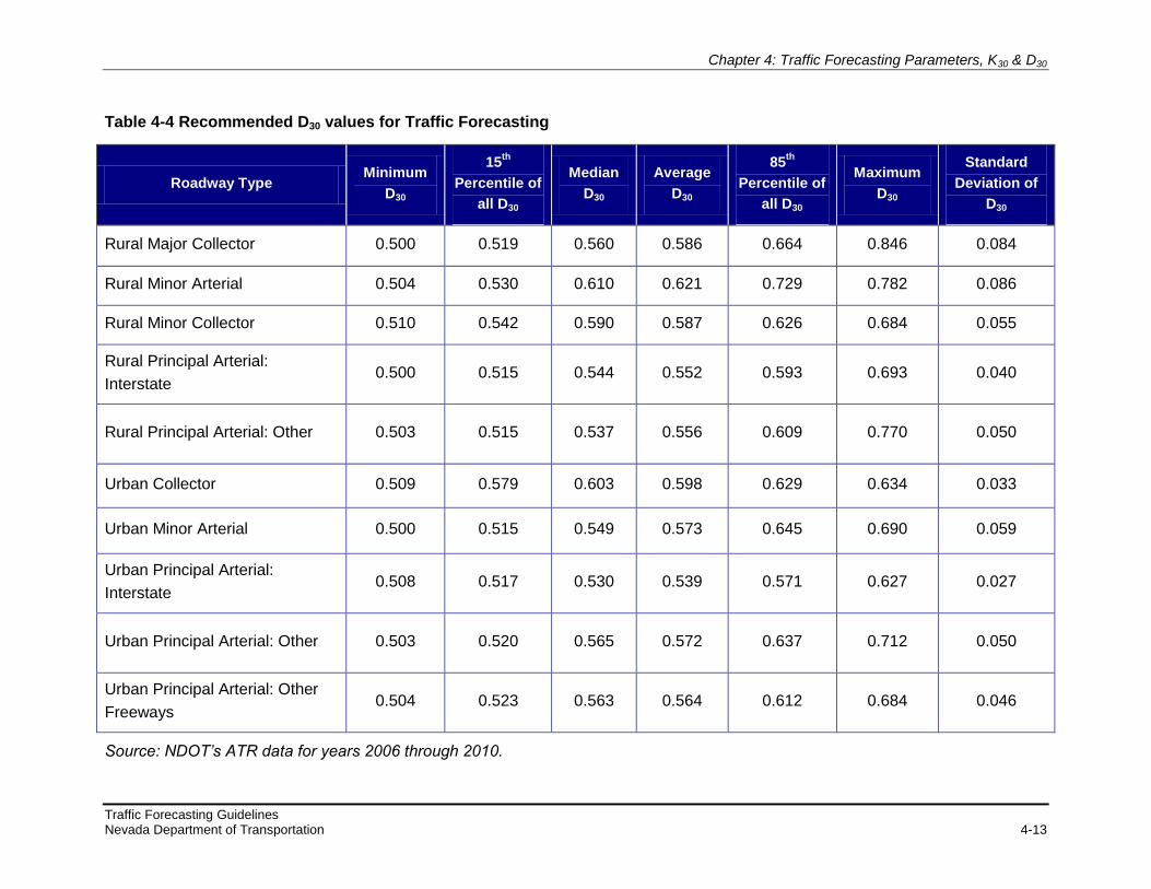
Chapter 4: Traffic Forecasting Parameters, K30 & D30
Traffic Forecasting Guidelines Nevada Department of Transportation 4-13
Table 4-4 Recommended D30 values for Traffic Forecasting
Roadway Type Minimum
D30
15th
Percentile of
all D30
Median
D30
Average
D30
85th
Percentile of
all D30
Maximum
D30
Standard
Deviation of
D30
Rural Major Collector 0.500 0.519 0.560 0.586 0.664 0.846 0.084
Rural Minor Arterial 0.504 0.530 0.610 0.621 0.729 0.782 0.086
Rural Minor Collector 0.510 0.542 0.590 0.587 0.626 0.684 0.055
Rural Principal Arterial:
Interstate 0.500 0.515 0.544 0.552 0.593 0.693 0.040
Rural Principal Arterial: Other 0.503 0.515 0.537 0.556 0.609 0.770 0.050
Urban Collector 0.509 0.579 0.603 0.598 0.629 0.634 0.033
Urban Minor Arterial 0.500 0.515 0.549 0.573 0.645 0.690 0.059
Urban Principal Arterial:
Interstate 0.508 0.517 0.530 0.539 0.571 0.627 0.027
Urban Principal Arterial: Other 0.503 0.520 0.565 0.572 0.637 0.712 0.050
Urban Principal Arterial: Other
Freeways 0.504 0.523 0.563 0.564 0.612 0.684 0.046
Source: NDOT’s ATR data for years 2006 through 2010.

Chapter 4: Traffic Forecasting Parameters, K30 & D30
Traffic Forecasting Guidelines Nevada Department of Transportation 4-14
4.8. Nonstandard K30 and D30 Values
If K30 and D30 values lower than NDOT’s 15th percentile values are to be used, or if D30 values
lower than 0.52 are to be used, then prior approval of NDOT is required before continuing the
traffic forecasting process.
4.9. Documenting Traffic Forecasts
As noted, the adopted methodology and underlying assumptions involved in estimating future
K30 and D30 values is to be clearly documented in the traffic forecast memorandum. All rationale
behind any adjustments made to the initial K30 and D30 values as well as the final values are
also to be documented in the traffic forecast memorandum.

Chapter 5 Traffic Forecasting with Travel Demand Models
Traffic Forecasting Guidelines Nevada Department of Transportation 5-1
5. Traffic Forecasting with Travel Demand Models
This chapter provides guidance on how to apply the outputs from a travel demand model when
developing traffic forecasts. As such, this chapter presents the following:
An overview of travel demand models;
The travel demand models that are available in the State;
The process to evaluate model output, methods for reviewing the accuracy of travel
demand model outputs; and
The information needed for the traffic forecast memorandum.
5.1. Overview of Travel Demand Models
Regional travel demand models are widely accepted planning tools that produce forecasts of
travel based on future estimates of population and employment. The primary purpose of a
regional travel demand model is to provide system-level traffic forecasts used to identify
transportation needs and future travel conditions. The resulting system travel demand forecasts
provide a basis for the more detailed evaluation required for specific project developments.
Travel demand models can be useful tools in developing the traffic projections. However, since
travel demand models are “planning” versus “design” tools, the system-level traffic projections
must be properly evaluated for reasonableness and consistency in light of current conditions
and those indicated by trends (see Chapter 6 of these Guidelines).
Travel demand models are typically developed and maintained by MPOs or local jurisdictions. A
regional travel demand model is calibrated and validated for the model calibration year, using
empirical traffic data from local origin and destination travel studies, traffic counts, transit
boarding volumes, journey-to-work and American Community Survey data from the US Census,
and other available travel behavior data. Calibration involves the adjustment of travel demand
model parameters so that predicted travel matches observed travel in the model calibration
year. Validation involves testing the predictive travel demand model data against additional
empirical data for the model calibration year. Calibration/validation is an iterative process until
the model’s system-wide results fall within an acceptable range of error.
A travel demand model is then used to forecast future volumes using population and
employment projections and the planned transportation network for a future year. The travel
demand model parameters are not to be modified from the model calibration year set-up. The
travel demand model for the model calibration year may be updated to create a base year
model. The base year is as close as possible to the existing year and the base year travel
demand model is validated using traffic volumes. This base year model is the basis for traffic
forecasts.
Figure 5-1 illustrates the process of traffic forecasting based on travel demand model output,
which is expanded upon in the subsequent sections of this chapter. Assumptions for typical

Chapter 5: Traffic Forecasting with Travel Demand Models
Traffic Forecasting Guidelines Nevada Department of Transportation 5-2
types of projects are provided, however, the analyst is cautioned concerning generalizations
because some projects could require (or warrant) a higher level of accuracy due to project-
specific circumstances.
The methodology of using travel demand model outputs for traffic forecasting is to be used for
planning, environmental analysis, and design projects. For operational analysis projects,
because the analysis years are usually within five years into the future, NDOT’s hourly count
data are to be the primary source for traffic forecasting. The traffic forecasting process, in this
case, would involve conducting a historical trend projection analysis, which is explained in
Chapter 6 of these Guidelines.

Chapter 5: Traffic Forecasting with Travel Demand Models
Traffic Forecasting Guidelines Nevada Department of Transportation 5-3
Begin
Compare base year model AADT with base year AADT observed in
the study area
Base year model traffic volume
outputs
Do they meet
consistency thresholds?
Refine model to better reflect base year conditions in
the study area
Yes
No
Update model to incorporate future year
roadway network changes
Execute future year model
Compare future year model AADT with future
year AADT from historical trend projection
Perform historical data trend
projection for check/validation
Yes
No
Document traffic forecast and assumptions
Are there any valid reasons
for the forecast differences?
No
Yes
Request guidance from NDOT. Implement guidance
Future year model outputs
Future year traffic from
historical trends
Will (further) model
refinements be cost-effective
to improve model results?
Yes
No
Update model to incorporate future year roadway network
changes
Adjust model outputs using procedures consistent with
NCHRP Report 255
Adjusted future year outputs
Are the forecasts
reasonable?
Compare adjusted future year model AADT with future year AADT from
historical trend projection
Execute future year model
Use model output to proceed with developing
forecast
Proceed with model based approach or select output from traffic forecasting without travel demand models (historical trend projection). Document reasons for selection of either approach
Figure 5-1 Traffic Forecasting with Travel Demand Models
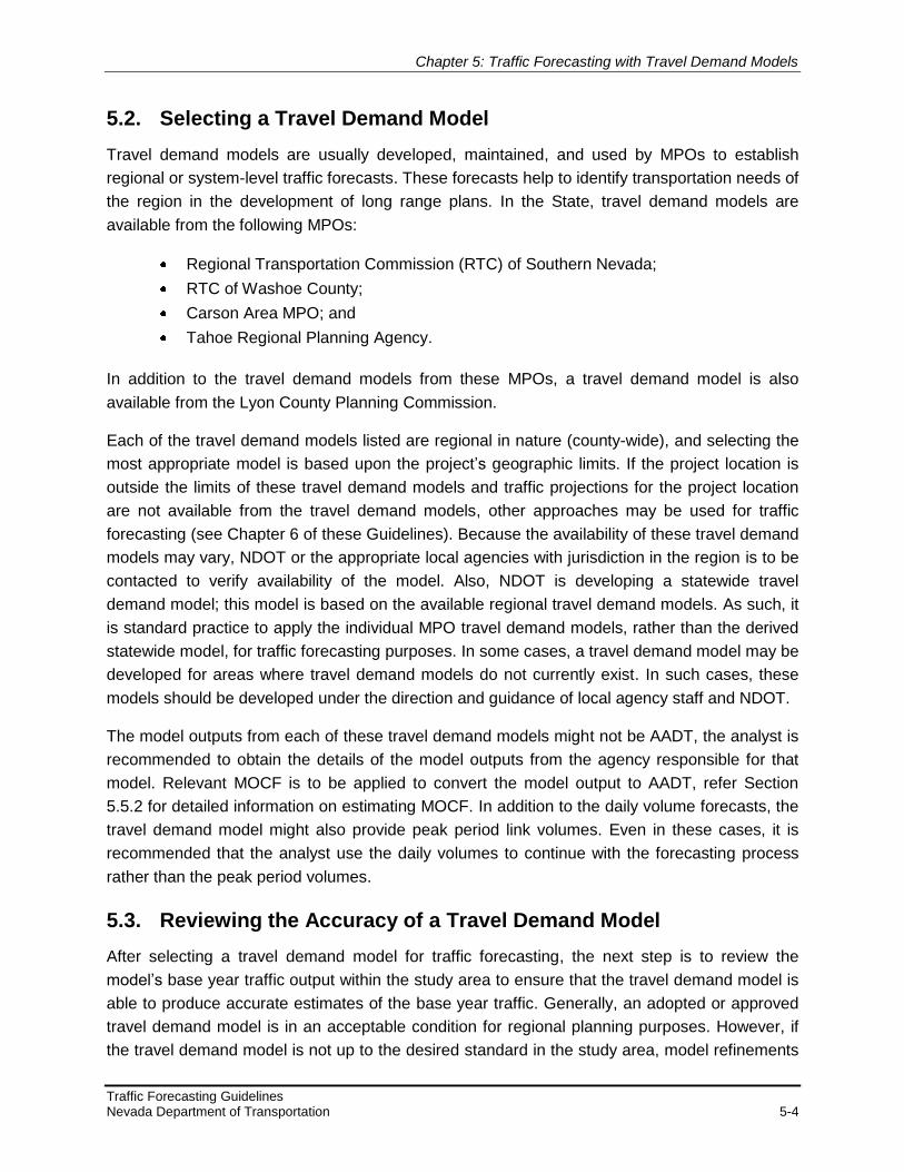
Chapter 5: Traffic Forecasting with Travel Demand Models
Traffic Forecasting Guidelines Nevada Department of Transportation 5-4
5.2. Selecting a Travel Demand Model
Travel demand models are usually developed, maintained, and used by MPOs to establish
regional or system-level traffic forecasts. These forecasts help to identify transportation needs of
the region in the development of long range plans. In the State, travel demand models are
available from the following MPOs:
Regional Transportation Commission (RTC) of Southern Nevada;
RTC of Washoe County;
Carson Area MPO; and
Tahoe Regional Planning Agency.
In addition to the travel demand models from these MPOs, a travel demand model is also
available from the Lyon County Planning Commission.
Each of the travel demand models listed are regional in nature (county-wide), and selecting the
most appropriate model is based upon the project’s geographic limits. If the project location is
outside the limits of these travel demand models and traffic projections for the project location
are not available from the travel demand models, other approaches may be used for traffic
forecasting (see Chapter 6 of these Guidelines). Because the availability of these travel demand
models may vary, NDOT or the appropriate local agencies with jurisdiction in the region is to be
contacted to verify availability of the model. Also, NDOT is developing a statewide travel
demand model; this model is based on the available regional travel demand models. As such, it
is standard practice to apply the individual MPO travel demand models, rather than the derived
statewide model, for traffic forecasting purposes. In some cases, a travel demand model may be
developed for areas where travel demand models do not currently exist. In such cases, these
models should be developed under the direction and guidance of local agency staff and NDOT.
The model outputs from each of these travel demand models might not be AADT, the analyst is
recommended to obtain the details of the model outputs from the agency responsible for that
model. Relevant MOCF is to be applied to convert the model output to AADT, refer Section
5.5.2 for detailed information on estimating MOCF. In addition to the daily volume forecasts, the
travel demand model might also provide peak period link volumes. Even in these cases, it is
recommended that the analyst use the daily volumes to continue with the forecasting process
rather than the peak period volumes.
5.3. Reviewing the Accuracy of a Travel Demand Model
After selecting a travel demand model for traffic forecasting, the next step is to review the
model’s base year traffic output within the study area to ensure that the travel demand model is
able to produce accurate estimates of the base year traffic. Generally, an adopted or approved
travel demand model is in an acceptable condition for regional planning purposes. However, if
the travel demand model is not up to the desired standard in the study area, model refinements

Chapter 5: Traffic Forecasting with Travel Demand Models
Traffic Forecasting Guidelines Nevada Department of Transportation 5-5
are necessary to update the travel demand model to an acceptable standard for project or
corridor-specific traffic forecasting purposes. The travel demand model is to be evaluated,
refined, and validated, as appropriate, to ensure that it can accurately forecast future traffic
volumes within the study area. The process also includes a review of available land use,
socioeconomic, and transportation network data to be used in the travel demand model, and
this review is to be documented and approved prior to its use.
5.3.1. Evaluating the Base Year Conditions
Reviewing the base year travel demand model ensures that the model is capable of replicating
base year conditions and, as an extension, future year conditions in the study area. Validating
the base year travel demand model allows the analyst to compare base year counts to the
modeled volumes. It is important to establish the travel demand model’s output in comparison
with the field data available. Because travel demand models can vary significantly, the agency
responsible for developing and maintaining the travel demand model must be contacted to
establish the exact model output. As noted, any modifications made to the travel demand model
output and the calculation of the MOCF must be documented in the traffic forecast
memorandum.
5.3.2. Refining the Base Year Travel Demand Model
When evaluating the travel demand model for base year conditions, if the model outputs are
found to vary from the field count data, base year refinements are necessary to ensure that the
travel demand model best reflects the actual conditions in the study area. The following is a
series of refinements that are commonly used to accomplish this.
The network is to be updated to ensure proper representation of roadways through
the inclusion of parallel roadway links, collector, and other secondary roadways
within the study area. Acceptable refinements include changes in roadway type, area
type, and the number of lanes.
The TAZs centroid connectors and their location are to be examined and adjusted if
necessary.
The socioeconomic base year data in the TAZs is to be reviewed within the study
area. Trips generated by prominent activity generators are to be compared to actual
traffic counts. If discrepancies are found from observed conditions, then coordination
with the MPO must occur to obtain consent and approval to make TAZ-related
socioeconomic modifications.
The following sections further detail the list above. Additionally, any refinement must include just
cause, and any refinement made to the travel demand model network or socioeconomic
assumptions must be clearly documented in the traffic forecast memorandum.

Chapter 5: Traffic Forecasting with Travel Demand Models
Traffic Forecasting Guidelines Nevada Department of Transportation 5-6
5.3.2.1. Base Year Socioeconomic Land Use Data Refinements
The base year land use data is to be analyzed within the study area for accuracy and
consistency with local comprehensive plans. When doing this, local planning agencies and
MPOs are to be contacted to verify the socioeconomic land use data. Furthermore, all existing
TAZs are to be analyzed based on the size and the number of trips each TAZ generates within
the study area. Trip end summaries for zones of interest in the study area are also to be
evaluated for reasonableness. It may be necessary to refine the existing TAZ structure to obtain
a better assignment, although special care must be taken to correctly code the new centroid
connectors. Though some data may be refined, the analyst must be aware that population,
employment, and other totals for the entire travel demand model cannot be changed. These
totals must continue to reflect the adopted RTP totals.
5.3.2.2. Base Year Network Refinements
The travel demand model’s base year network within the study area is to be evaluated to ensure
that all major roadways are coded appropriately. Additional roadways may need to be added to
the network to provide better loading points for newly created TAZs/centroid connectors, as well
as to allow for an improved path building process. The coding of all roadways within the study
area is to be verified with regards to their roadway type and number of lanes.
5.3.2.3. Base Year Count Refinements
An analysis is to be conducted to identify whether a sufficient amount of count data is available
within the study area. If critical links are missing counts, then additional counts are to be
obtained. If any roadways have been added to the network, the availability of counts is to be
checked for these added roadways. An analysis is also conducted to add cutlines, which may
require additional counts, within the study area for quicker analysis of the accuracy of the
distribution patterns. These additional counts would have to be adjusted to the base year of the
study, as well as to the units the travel demand model uses (axle adjustments, AADT, ADT,
AWDT, etc.). It should be noted that this approach may be a costly endeavor and may not
always be feasible or desirable, based on the production schedule of certain projects.
5.3.3. Determining the Necessity and Feasibility of Further Refinements
After the appropriate base year travel demand model refinements have been incorporated, the
modified travel demand model is assessed for accuracy. The accuracy of the model is to be
evaluated to identify if the travel demand model outputs are consistent with real world
conditions. This accuracy assessment is to be conducted as explained in Section 5.3.4. If the
travel demand model outputs are found to be accurate and consistent with the real world
conditions within the study area, the analyst may proceed to Section 5.4 of these Guidelines to
apply the travel demand model for future year conditions. However, if the travel demand model
is found to be inconsistent even after the base year refinements, the analyst is to evaluate the
feasibility and cost-effectiveness of further refinements to the base year travel demand model. If

Chapter 5: Traffic Forecasting with Travel Demand Models
Traffic Forecasting Guidelines Nevada Department of Transportation 5-7
further refinements are feasible, the travel demand model is updated, and an accuracy
assessment is conducted again. Figure 5-1 provides the series of steps involved in base year
travel demand model refinements, determining the necessity and feasibility of further
refinements and the relevant subsequent steps.
5.3.4. Recommended Accuracy Levels (Consistency Thresholds)
After refining the travel demand model to improve its ability to reflect base year conditions, the
model outputs are tested against consistency thresholds. If the travel demand model outputs
meet the consistency thresholds, then the travel demand model can be applied for the future
year conditions, and the model outputs can be used for the traffic analysis. If the travel demand
model outputs do not meet the consistency thresholds, then the model outputs are to be
adjusted based on the industry standard NCHRP Report 255 procedures before proceeding to
the traffic analysis process. Table 5-1 and Table 5-2 list the consistency thresholds that are
required to be met.
Table 5-1 lists the percent deviation thresholds. This prescribes the extent by which the travel
demand model volume can differ from the field count and still be accurate enough to proceed
with the traffic forecasting process without adjusting the model outputs. Conceptually, model-
simulated link volumes are expected to be accurate enough to correctly determine the required
number of lanes for roadway design. This means that the acceptable error must be no more
than the service volume (at the design LOS) for one lane of traffic. This reference service
volume is a higher percentage of total traffic for low volume roads than for high volume roads.
The percent deviation between the NDOT counts and travel demand model volumes for each
link is calculated using the following formula where “i” corresponds to a link/segment in the
roadway network and “n” is the total number of links/segments, as expressed in the following
equation.
100Count
VolumeModelCountDeviationPercent
i
iii
Percent deviation values are to be calculated separately for each link across the cultines and for
each link along the project corridor. These percent deviation values are to be compared against
the maximum allowable percent deviation thresholds (Table 5-1) for the AADT range that the
subject links correspond to.
Table 5-2 lists the acceptable Coefficient of Variation of Root Mean Square Error (CV[RMSE])
thresholds for identifying the consistency between the travel demand model outputs and the
base year counts. The CV(RMSE) between the NDOT counts and travel demand model
volumes for each AADT range are calculated using the following formula where “i” corresponds
to a link/segment in the roadway network and “n” is the total number of links/segments, as
expressed in the following equation.
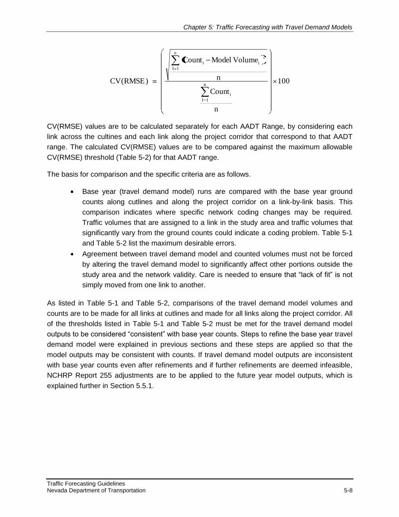
Chapter 5: Traffic Forecasting with Travel Demand Models
Traffic Forecasting Guidelines Nevada Department of Transportation 5-8
100
n
Count
n
VolumeModelCount
)RMSE(CVn
1I
i
n
1I
2
ii
CV(RMSE) values are to be calculated separately for each AADT Range, by considering each
link across the cultines and each link along the project corridor that correspond to that AADT
range. The calculated CV(RMSE) values are to be compared against the maximum allowable
CV(RMSE) threshold (Table 5-2) for that AADT range.
The basis for comparison and the specific criteria are as follows.
Base year (travel demand model) runs are compared with the base year ground
counts along cutlines and along the project corridor on a link-by-link basis. This
comparison indicates where specific network coding changes may be required.
Traffic volumes that are assigned to a link in the study area and traffic volumes that
significantly vary from the ground counts could indicate a coding problem. Table 5-1
and Table 5-2 list the maximum desirable errors.
Agreement between travel demand model and counted volumes must not be forced
by altering the travel demand model to significantly affect other portions outside the
study area and the network validity. Care is needed to ensure that “lack of fit” is not
simply moved from one link to another.
As listed in Table 5-1 and Table 5-2, comparisons of the travel demand model volumes and
counts are to be made for all links at cutlines and made for all links along the project corridor. All
of the thresholds listed in Table 5-1 and Table 5-2 must be met for the travel demand model
outputs to be considered “consistent” with base year counts. Steps to refine the base year travel
demand model were explained in previous sections and these steps are applied so that the
model outputs may be consistent with counts. If travel demand model outputs are inconsistent
with base year counts even after refinements and if further refinements are deemed infeasible,
NCHRP Report 255 adjustments are to be applied to the future year model outputs, which is
explained further in Section 5.5.1.

Chapter 5: Traffic Forecasting with Travel Demand Models
Traffic Forecasting Guidelines Nevada Department of Transportation 5-9
Table 5-1 Consistency Thresholds: Percent Deviation Thresholds for every Link across
Cutlines and all Project Corridor Links
AADT Range Maximum Allowable
Percent Deviation
< 50,000 ± 10%
50,000 - 249,999 ± 7.5%
≥ 250,000 ± 5%
Table 5-2 Consistency Thresholds: CV(RMSE) Thresholds for every Link across Cutlines
and all Project Corridor Links
AADT Range Maximum Allowable
CV(RMSE)
< 5,000 45%
5,000 – 9,999 35%
10,000 – 14,999 30%
15,000 – 19,999 25%
20,000 – 49,999 20%
> 50,000 10%

Chapter 5: Traffic Forecasting with Travel Demand Models
Traffic Forecasting Guidelines Nevada Department of Transportation 5-10
For the purpose of illustration, the travel demand model outputs for the region near Pyramid
Way, Washoe County, are used here and the accuracy of the model outputs is evaluated. The
travel demand model outputs from the 2008 RTC Washoe Interim Consensus Forecast (ICF)
Base Model are compared with field counts to determine whether the model outputs satisfy the
consistency thresholds.
This location falls under the purview of the travel demand model developed by the RTC of
Washoe County. Figure 5-2 shows a portion of the year 2008 model output and the link volumes
for a few segments; the models outputs are in 100’s of AWDT. Hence, the model outputs
(AWDT) were first converted to AADT by applying the MOCF (the methodology of estimation of
MOCF for a model is explained in Section 5.5.2).
Table 5-3 and Table 5-4 show the Model AADT and the actual AADT obtained from field counts
for each link along the project corridor. Table 5-3 shows the calculated percent deviation for
each link along the project corridor. Similarly, Table 5-4 shows the calculated CV(RMSE)
corresponding to each link along the project corridor estimated by AADT range.
Note that this illustrative accuracy assessment did not look at links across cutlines, the
comparison of travel demand model outputs with field counts should be done at all links across
cutlines too.
From Table 5-3 and Table 5-4, it can be seen that only one of the links meets the percent
deviation thresholds and none of the links meet the CV(RMSE) thresholds. Travel demand
model outputs are deemed inconsistent even if one of the links is found to exceed the
consistency thresholds. Thus, it was determined that the model outputs were not consistent with
the existing field counts and NCHRP Report 255 adjustments were deemed necessary. The
application of these adjustments is explained in Section 5.5.1.

Chapter 5: Traffic Forecasting with Travel Demand Models
Traffic Forecasting Guidelines Nevada Department of Transportation 5-11
Pyramid Way -
Queen Way to
Disc Drive
Pyramid Way - Disc
Drive to Los Altos
Parkway
Pyramid Way - Los
Altos Parkway to
Golden View Drive
Pyramid Way -
Golden View Drive
to Sparks Boulevard
Model Outputs are
100’s of AWDT
Figure 5-2 Sample Year 2008 Travel Demand Model Output Plot
Source: RTC Washoe

Chapter 5: Traffic Forecasting with Travel Demand Models
Traffic Forecasting Guidelines Nevada Department of Transportation 5-12
Table 5-3 Sample Percent Deviation Comparison along all Project Corridor Links
Segment Field Count Source Model AADT Actual AADT Percent
Deviation
Meets Consistency
Thresholds?
US-395: North of Parr NDOT Station #418
(2008 volume) 73,453 66,260 11% No
US-395: South of Parr NDOT Station #468
(2008 volume) 79,336 69,334 14% No
Pyramid Way: Queen Way to Disc
Drive
NDOT Station #340
(2008 volume) 54,662 43,594 25% No
Pyramid Way: Disc Drive to Los
Altos Parkway 2007 tube count 48,019 37,805 27% No
Pyramid Way: Los Altos Parkway to
Golden View Drive 2007 tube count 37,106 31,792 17% No
Pyramid Way: Golden View Drive to
Sparks Boulevard 2007 tube count 34,259 27,054 27% No
Pyramid Way: Sparks Boulevard to
Dolores Drive 2007 tube count 53,429 38,398 39% No
Pyramid Way: Dolores Drive to La
Posada Drive 2008 tube count 46,976 34,119 38% No
Pyramid Way: La Posada Drive to
Sunset Springs Lane 2007 tube count 26,003 18,368 42% No
Pyramid Way: Sunset Springs Lane
to Calle De La Plata 2007 tube count 17,272 12,778 35% No
Sun Valley Boulevard: South of
Dandini Boulevard
NDOT Station #344
(2008 volume) 25,338 23,188 9% Yes
Sun Valley Boulevard: North of
Dandini Boulevard
NDOT Station #345
(2007 volume) 39,953 32,859 22% No
Source: Jacobs, Pyramid Highway US 395 Connection

Chapter 5: Traffic Forecasting with Travel Demand Models
Traffic Forecasting Guidelines Nevada Department of Transportation 5-13
Table 5-4 Sample CV(RMSE) Comparison along all Project Corridor Links
AADT Range Segment Model AADT Actual AADT CV(RMSE) Meets Consistency
Thresholds?
10,000-14,999 Pyramid Way: Sunset Springs
Lane to Calle De La Plata 17,272 12,778 35% No
15,000-19,999 Pyramid Way: La Posada
Drive to Sunset Springs Lane 26,003 18,368 42% No
20,000-49,999
Pyramid Way: Queen Way to
Disc Drive 54,662 43,594
37%
No
Pyramid Way: Disc Drive to
Los Altos Parkway 48,019 37,805 No
Pyramid Way: Los Altos
Parkway to Golden View Drive 37,106 31,792 No
Pyramid Way: Golden View
Drive to Sparks Boulevard 34,259 27,054 No
Pyramid Way: Sparks
Boulevard to Dolores Drive 53,429 38,398 No
Pyramid Way: Dolores Drive to
La Posada Drive 46,976 34,119 No
Sun Valley Boulevard: South
of Dandini Boulevard 25,338 23,188 No
Sun Valley Boulevard: North of
Dandini Boulevard 39,953 32,859 No
>50,000
US-395: North of Parr 73,453 66,260
13%
No
US-395: South of Parr 79,336 69,334 No
Source: Jacobs, Pyramid Highway US 395 Connection

Chapter 5: Traffic Forecasting with Travel Demand Models
Traffic Forecasting Guidelines Nevada Department of Transportation 5-14
5.4. Applying the Travel Demand Model for Future Year Conditions
After reviewing the travel demand model for base year conditions, the model is ready to
determine the future year traffic forecasts. However, the future year travel demand model has to
reflect any refinements to the base year travel demand model. In addition, the network needs to
accurately reflect future year conditions. This section explains the methodology to prepare the
travel demand model to reflect future year conditions.
5.4.1. Modifying Future Year Network and Land Use
When forecasting interim and design year traffic, it may be necessary to incorporate any
refinements in socioeconomic land use and/or changes in the network that is not reflected in the
approved interim and design year data sets. Similar to the incorporation of base year travel
demand model refinements, these changes are not to be made without the coordination and
approval from the agency responsible for the travel demand model. Changes made to the travel
demand model must be consistent with the methodology prescribed by the agency responsible
for the travel demand model and are to be fully documented in the traffic forecast memorandum
in a manner that would allow another individual to make the same changes and obtain the same
results. This material is then reviewed with NDOT and the agency responsible for the travel
demand model to obtain consensus on the results.
5.4.2. Evaluating Future Year Conditions
In order to forecast traffic for a given year, appropriate future year data inputs are required. For
each of the future analysis years, the following travel demand model inputs are to be
summarized:
Transportation network, and
Socioeconomic/land use data.
Each of these factors is to be updated to reflect the approved elements of the MPO’s financially
feasible long range plan along with the planned development mitigation infrastructure
improvements anticipated to be in place in each analysis year. Because the timing of land use
and network changes is not usually a known quantity, it may be appropriate to use the modeled
data in a regression analysis with the historical data in order to obtain an AADT for any given
year.
5.5. Executing the Travel Demand Model and Evaluating Outputs
After the travel demand model has been appropriately updated to reflect the future year
conditions, the next step is to execute the model. Guidelines regarding the execution of a travel
demand model are to be obtained from the agency responsible for the travel demand model and
must be followed accordingly. For the sake of evaluating outputs, the outputs from the travel
demand model are compared with results from a historical trend projection analysis. Care is

Chapter 5: Traffic Forecasting with Travel Demand Models
Traffic Forecasting Guidelines Nevada Department of Transportation 5-15
necessary when evaluating the travel demand model outputs to ensure that the model outputs
are the same type as the results from the historical trend projection. For example, if the travel
demand model outputs are AWDT and the historical trend projection uses AADT, then the
model outputs must first be converted to AADT.
5.5.1. Adjusting Travel Demand Model Output using NCHRP Report 255
Procedures (If Necessary)
The following is to be applied only if the base year travel demand model was found to be
inconsistent with real world conditions, and further model refinements were deemed necessary.
Correspondingly, this section explains the NCHRP Report 255 guidelines for adjusting the travel
demand model outputs in such cases, so that the future year model outputs are relevant and
accurate.
In general, there are three procedures described in NCHRP Report 255 for adjustment of link
volumes obtained from computerized travel demand volume forecasts. These three methods
are the ratio adjustment method, the difference adjustment method, and the combination
adjustment method. The purpose of each method is to adjust the future year link assignments to
account for possible assignment errors.
For the purpose of illustration, travel demand model outputs are used for the region near
Pyramid Way in Washoe County. This location falls under the purview of the travel demand
model developed by the RTC of Washoe County. The travel demand model outputs from the
2008 RTC Washoe Interim Consensus Forecast (ICF) Base Model and the Year 2030 No-Build
scenario are used to illustrate the adjustments.
Figure 5-2 shows a portion of the 2008 travel demand model output and the link volumes for a
few segments. The model outputs are in 100s of AWDT. Table 5-5 lists examples of the
application of these procedures to adjust travel demand model outputs. In this example,
adjustments have been made to the travel demand model output AWDT, but the procedures
described may also be applied to the model outputs after being converted to AADT (i.e., after
applying the MOCF to the model outputs).
5.5.1.1. Ratio Adjustment Method
The ratio adjustment method can be described as a growth factor method where the growth
between the base year’s and future year’s travel demand model outputs is applied to the field
measured traffic counts. This method can generate erroneous or problematic results if the field
traffic count is significantly greater than the travel demand model reported traffic volume or vice
versa. In such a case, NCHRP Report 255 recommends using the difference adjustment
method.
In Table 5-5, the ratio adjustment method has been applied as follows:

Chapter 5: Traffic Forecasting with Travel Demand Models
Traffic Forecasting Guidelines Nevada Department of Transportation 5-16
countyearBasevolumeelmodyearBase
volumeelmodyearFuture
5.5.1.2. Difference Adjustment Method
The difference adjustment method provides adjusted volumes on each link by the addition of the
difference (or increment) between the base year travel demand model and future year travel
demand model to the field measured traffic volume. This method can generate problematic
results if the difference is less than zero, which may lead to a (impossible) negative adjusted
value for future traffic. In such a case, NCHRP Report 255 recommends using the ratio
adjustment method.
In Table 5-5, the difference adjustment method has been applied as follows:
countyearBasevolumeelmodyearBasevolumeelmodyearFuture
5.5.1.3. Combination Adjustment Method
The combination adjustment method suggests taking the average of the values obtained by the
ratio adjustment method and the difference adjustment method. If either of the ratio adjustment
or difference adjustment method is found to produce erroneous or problematic results, then it is
recommended not to use the combination adjustment method. Rather, the analyst is to use the
method that provides the most reasonable results.
In all, the analyst is to apply engineering judgment on a case-by-case basis when choosing the
most suitable method of adjustment. It is also acceptable to apply the most suitable method on
a link-by-link basis, if the analyst determines that such an application will yield the most
reasonable results.

Chapter 5: Traffic Forecasting with Travel Demand Models
Traffic Forecasting Guidelines Nevada Department of Transportation 5-17
Table 5-5 Sample NCHRP Report 255 Adjustments to the Travel Demand Model Output
Roadway Segment
Year 2008:
Actual
AWDT
Year 2008:
Model
Output
AWDT
Year 2030:
Model Output
AWDT
Year 2030 Model AWDT after NCHRP Report 255
Adjustments
Ratio
Adjustment
Method
Difference
Adjustment
Method
Combination
Adjustment
Method
US-395: North of Parr 69,789 77,400 155,000 139,760 147,390 143,580
US-395: South of Parr 73,027 83,600 166,900 145,800 156,330 151,070
Pyramid Way: Queen Way to
Disc Drive 45,916 57,600 63,200 50,390 51,520 50,960
Pyramid Way: Disc Drive to Los
Altos Parkway 39,819 50,600 53,900 42,420 43,120 42,770
Pyramid Way: Los Altos
Parkway to Golden View Drive 33,485 39,100 51,400 44,020 45,790 44,910
Pyramid Way: Golden View
Drive to Sparks Boulevard 28,495 36,100 48,100 37,970 40,500 39,240
Pyramid Way: Sparks
Boulevard to Dolores Drive 40,443 56,900 60,600 43,080 44,150 43,620
Pyramid Way: Dolores Drive to
La Posada Drive 35,936 49,500 46,300 33,620 32,740 33,180
Sun Valley Boulevard - South
of Dandini Boulevard 24,423 26,700 53,100 48,580 50,830 49,710
Sun Valley Boulevard - North of
Dandini Boulevard 34,609 42,100 62,900 51,710 55,410 53,560
Source: Jacobs, Pyramid Highway US 395 Connection
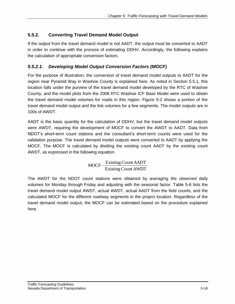
Chapter 5: Traffic Forecasting with Travel Demand Models
Traffic Forecasting Guidelines Nevada Department of Transportation 5-18
5.5.2. Converting Travel Demand Model Output
If the output from the travel demand model is not AADT, the output must be converted to AADT
in order to continue with the process of estimating DDHV. Accordingly, the following explains
the calculation of appropriate conversion factors.
5.5.2.1. Developing Model Output Conversion Factors (MOCF)
For the purpose of illustration, the conversion of travel demand model outputs to AADT for the
region near Pyramid Way in Washoe County is explained here. As noted in Section 5.5.1, this
location falls under the purview of the travel demand model developed by the RTC of Washoe
County, and the model plots from the 2008 RTC Washoe ICF Base Model were used to obtain
the travel demand model volumes for roads in this region. Figure 5-2 shows a portion of the
travel demand model output and the link volumes for a few segments. The model outputs are in
100s of AWDT.
AADT is the basic quantity for the calculation of DDHV, but the travel demand model outputs
were AWDT, requiring the development of MOCF to convert the AWDT to AADT. Data from
NDOT’s short-term count stations and the consultant’s short-term counts were used for the
validation purpose. The travel demand model outputs were converted to AADT by applying the
MOCF. The MOCF is calculated by dividing the existing count AADT by the existing count
AWDT, as expressed in the following equation.
AWDTCountExisting
AADTCountExistingMOCF
The AWDT for the NDOT count stations were obtained by averaging the observed daily
volumes for Monday through Friday and adjusting with the seasonal factor. Table 5-6 lists the
travel demand model output AWDT, actual AWDT, actual AADT from the field counts, and the
calculated MOCF for the different roadway segments in the project location. Regardless of the
travel demand model output, the MOCF can be estimated based on the procedure explained
here.

Chapter 5: Traffic Forecasting with Travel Demand Models
Traffic Forecasting Guidelines Nevada Department of Transportation 5-19
Table 5-6 Sample Calculation of MOCF
Roadway Segment Actual Count Source Actual
AWDT
Actual
AADT
Actual AADT
to Actual
AWDT (MOCF)
Model
Output
(AWDT)
Converted
Model Volume
(Model AADT)
US-395: North of Parr NDOT Station #418
(2008 volume) 69,789 65,210 0.934 77,400 73,453
US-395: South of Parr NDOT Station #468
(2008 volume) 73,027 67,957 0.931 83,600 79,336
Pyramid Way: Queen Way to
Disc Drive
NDOT Station #340
(2008 volume) 45,916 44,137 0.961 57,600 54,662
Pyramid Way: Disc Drive to Los
Altos Parkway 2007 tube count 39,819 - - 50,600 48,019
Pyramid Way: Los Altos
Parkway to Golden View Drive 2007 tube count 33,485 - - 39,100 37,106
Pyramid Way: Golden View
Drive to Sparks Boulevard 2007 tube count 36,100 28,495 - - 34,259
Pyramid Way: Sparks
Boulevard to Dolores Drive 2007 tube count 56,300 40,443 - - 53,429
Pyramid Way: Dolores Drive to
La Posada Drive 2008 tube count 49,500 35,936 - - 46,976
Sun Valley Boulevard: South of
Dandini Boulevard
NDOT Station #344
(2008 volume) 24,423 22,863 0.936 26,700 25,338
Sun Valley Boulevard: North of
Dandini Boulevard
NDOT Station #345
(2007 volumes) 34,609 34,083 0.985 42,100 39,953
Average MOCF 0.949
Source: Jacobs, Pyramid Highway US 395 Connection

Chapter 5: Traffic Forecasting with Travel Demand Models
Traffic Forecasting Guidelines Nevada Department of Transportation 5-20
5.5.2.2. Converting AWDT to AADT
The MOCFs were calculated corresponding to each of the NDOT short-term count stations in
the project location. In the example (Table 5-6), five NDOT count stations were present in the
project location. The MOCFs corresponding to each of these count stations were averaged to
obtain a project-wide MOCF. This project-wide MOCF was applied to the travel demand model
output AWDTs to obtain the AADT projections from the model. The travel demand model
AADTs are calculated from the AWDTs using the following equation:
MOCFAWDTModelAADTModel
The “Converted Model Volume” column of Table 5-6 lists the travel demand model outputs
converted to AADT using the calculated MOCF.
This illustration explained the conversion of travel demand model output AWDT to AADT. But,
this same procedure may be appropriately applied even if the travel demand model outputs are
a different quantity.
5.5.3. Comparison of Model Forecasts with Historical Trend Projection Results
Once the travel demand model-predicted future year traffic volumes are available, a historical
trend projection analysis is to be completed for comparison with the model results. A historical
trend projection analysis is done based on one or more of the following: available historical
traffic counts, population growth, employment, gasoline sales, or other appropriate growth
indicators. While comparing the travel demand model output volumes with historical trend
projection results, engineering judgment is to be applied in determining “reasonableness.” The
trend in the change of traffic from both the procedures is to be compared, and the rationale and
justification behind the judgment are to be documented in the traffic forecast memorandum. If
the comparison fails the test of reasonableness, the causes must be identified. An example of a
traffic forecast that could be higher than the historical trend would be the addition of lanes or
new land development in the study area. An example of a traffic forecast that could be lower
than the historical trend would be a future congested roadway identified by the preliminary
capacity analysis. These factors and other relevant factors are to be considered when preparing
the historical trend projections. The methodology to complete a historical trend projection is
explained further in Chapter 6 of these Guidelines.
Future year traffic volumes cannot be validated against existing traffic counts. The modeled
volume changes for each year of analysis and for each alternative network are to be evaluated
against the expected changes. Although expected changes cannot be accurately quantified,
approximate changes are to be estimated. For example, if the region’s growth is expected to
continue, freeway volumes are expected to increase with some relationship to the trend. The
percentage of change between years would be expected to be relatively constant unless some
special factors affect the growth, such as improvement of parallel roadways.

Chapter 5: Traffic Forecasting with Travel Demand Models
Traffic Forecasting Guidelines Nevada Department of Transportation 5-21
The travel demand model-generated volumes for the future years are to be reviewed for logical
traffic growth rates. The general growth trends and growth rates prevalent in the area can be
identified by the historical trend projection analysis. The future year travel demand model
volumes are compared against the appropriate historical count data. If an unexplained growth
rate exists, a thorough review of the base and future year land use, socioeconomic data, and
network coding must be performed. Logical reasons for any anomalies are to be documented in
the traffic forecast memorandum. A careful comparison is required, especially for urbanized
areas where growth may be higher along undeveloped corridors, although on an area-wide
basis, it may be much lower. Care must be applied to ensure that similar types of traffic outputs
are compared. For instance, if a travel demand model outputs AWDT and the historical trend
projection is made for AADT, the travel demand model outputs are to first be converted to AADT
before comparison (see Section 5.5.2 of these Guidelines).
Travel demand models frequently provide insight into traffic route selection that might not be
readily apparent. However, if the travel demand model outputs are found to be unreasonable
when compared to the historical trend projection results, valid reasons for the variation in the
results must be identified. If valid reasons for the inconsistency cannot be determined, then
guidance is to be requested from NDOT, and this guidance is to be followed in the traffic
forecasting process. Valid explanations for differences between the historical trend and travel
demand model forecast may include land use changes, new roadways, congested conditions, or
other considerations that may not be reflected in either the travel demand model or the historical
trend analysis projection. All of these issues must be taken into consideration when evaluating
the traffic forecasts. As noted, complete documentation of the traffic projection process,
including reasonableness evaluation, is to be included in the traffic forecast memorandum.
5.6. Obtaining Design Year AADT from the Travel Demand Model’s
Future Year AADT Estimates
In some cases, the travel demand model’s future years may not match the design year of the
transportation project. In these cases, the design year is usually within a couple of years of the
travel demand model’s future year. Subsequent to following the guidelines explained in the
previous sections of this chapter, the AADT estimates that were prepared for the travel demand
model’s future year are to be used to obtain the project design year AADT.
Compound annual growth rates are to be estimated at each of the study locations, between the
interim year and the future year AADT estimates. If AADT estimates are unavailable for an
interim year, the compound annual growth rates are to be calculated between the base year and
the future year AADT estimates. The compound annual growth rates are to be calculated using
the following formula, where “r” is the desired compound annual growth rate being calculated
and “n” is the number of years between the “interim year” and the “future year”.

Chapter 5: Traffic Forecasting with Travel Demand Models
Traffic Forecasting Guidelines Nevada Department of Transportation 5-22
1AADTyearInterim
AADTyearFuturer
n
1
These compound annual growth rates are to be applied to the future year AADT estimates
obtained from the travel demand model to estimate the design year AADT. Depending on
whether the design year is before or beyond the travel demand model future year, the
compound annual growth rates are to be applied according to either of the two following
formulae.
If the design year is before the travel demand model future year, then
nr1
AADTyearFutureAADTyearDesign
Or, if the design year is beyond the travel demand model future year, then
nr1AADTyearFutureAADTyearDesign
In both these formulae, “r” is the compound annual growth rate calculated in the previous step
and “n” is the number of years between the “future year” and the “design year”.
For the purpose of illustration, consider the following case of the estimation of the design year
AADT for a particular study location.
Interim year (year 2025) AADT at a study location is 9,640
Future year (year 2035) AADT at the same study location is 12,220
The design year of the transportation project is year 2033 and AADT is to be
obtained for this study location for the design year
Using the formulae listed above, the compound annual growth rate for the location between
year 2025 and year 2035 is
024.019640
12220r
10
1
Applying this compound annual growth rate to estimate the design year AADT,
654,11)024.01(
12220AADT)2033year(yearDesign
2
Hence, the design year AADT = 11,654 = 11,500 (after rounding)

Chapter 5: Traffic Forecasting with Travel Demand Models
Traffic Forecasting Guidelines Nevada Department of Transportation 5-23
5.7. Documenting Traffic Forecasts
After the travel demand model results are validated and the traffic forecast is finalized, the next
step is to document the forecast. Every assumption made in the traffic forecasting process and
every decision made at the decision points shown in Figure 5-1 are to be documented in the
traffic forecast memorandum following the guidelines listed in Section 1.7 and Section 1.8. The
plots of the study area are to be maintained in the file. Tabulation of the forecasts for the interim
and design year are also to be included in an individual section of the traffic forecast
memorandum. Appropriate documentation of the methodology, calculation of MOCFs, model
accuracy assessment and comparison against consistency thresholds, details of NCHRP
Report 255 adjustments applied and reasonableness evaluation with historical trend projection
analyses are to be included in the traffic forecast memorandum. Schematic diagrams of the
project are to be developed as needed to clearly convey the forecasts. AADT, peak hour link
volumes, peak hour turning movements, K30, D30, and T% should be documented.

Chapter 6 Traffic Forecasting without a Travel Demand Model
Traffic Forecasting Guidelines Nevada Department of Transportation 6-1
6. Traffic Forecasting without a Travel Demand Model
This chapter provides the methodology and procedures for developing traffic forecasts when a
usable travel demand model is not available for the project location. The chapter presents:
An overview of historical trend projection analyses to forecast traffic in an area
without a travel demand model;
The procedures for performing historical trend projection analyses; and
Various other references that can assist when forecasting traffic in an area without a
travel demand model.
The chapter concludes with a sample case of how to perform a historical trend projection
analysis.
6.1. Overview of Historical Trend Projection Analyses
For areas without a travel demand model, traffic forecasts are normally based on historical
trends of traffic count data, and growth rates may also be developed (if available) through
gasoline consumption reports, census data, and working with the county, city, and their
comprehensive plans. Future growth rates can be obtained using nearby metropolitan area
growth projections, Statewide plan projections, and information from local comprehensive plans.
When historical AADT data is used, a regression analysis is to be performed using the most
recent ten years of data. Depending on the availability of data, the regression analysis is
conducted using as much historical data as possible. Caution is needed to negate counts that
might be obviously out of sync with other years. Some of the most commonly used growth
trends are linear, logarithmic, and exponential, and the use of a particular trend depends on the
historical traffic data and existing and expected land use characteristics of the project location
and the level of “fit” of a particular trend for the available historical data.
It is important to consider the capacity of the roadway when creating the projection for future
years. Projections are to show traffic demand and not be constrained because the roadway
itself becomes constrained as traffic becomes congested. If the demand is for a six-lane
roadway and a four-lane roadway is being designed, then the traffic forecast memorandum is to
note that four lanes will not be adequate for a 20-year design. Subsequently, steps are to be
taken to address the potential short fall. To arbitrarily constrain traffic does nothing to address or
mitigate future congestion.
6.2. Procedures for Performing Historical Trend Projection Analyses
This section explains the methodology and steps to perform a historical trend projection analysis
to forecast traffic in an area without a travel demand model.

Chapter 6: Traffic Forecasting without a Travel Demand Model
Traffic Forecasting Guidelines Nevada Department of Transportation 6-2
6.2.1. Assembling the Data
When available and applicable, the analyst is to assemble the following items for preparing a
traffic forecast where a travel demand model is not available (also see Section 6.4 of these
Guidelines):
Mapping or other roadway location drawings of the roadway requiring traffic
projections (e.g., a project location map);
Graphical representation of existing lane arrangements (e.g., aerial photography and
intersection sketches);
Resources for determining traffic growth trends, including:
o Historical traffic count data (Existing year plus nine earlier years of mainline
traffic is considered the minimum, but if ten years of data is not available, existing
year plus four or more earlier years of mainline and/or intersection approach
volumes are necessary), and
o Current and historical population data (if available);
o Gas sales records (if available);
Traffic factors, including K30, D30, and T%;
RTP or LGCP (land use and traffic circulation elements);
Description of existing and future land uses that contribute traffic that would use the
proposed roadway;
Current HCM and relevant software;
The opening year, interim year and design year;
Adjacent or nearby metropolitan area growth projections; and
Statewide plan forecasts.
6.2.2. Establishing Traffic Growth Trends
When establishing traffic growth trends, the analyst is to use the following approaches.
Plot historical AADT at a convenient scale with traffic volume on the y-axis and year
of count on the x-axis (leaving room for design year and traffic growth) (see Figure
6-1).
Use least squares regression analysis combined with graphical representation of
traffic growth trends. The R-squared statistic associated with the growth trend is to
be reported.
If historical count data are insufficient, prepare a similar analysis of alternative
indicators that are available (e.g., gas sales data, population data).
Using historical data (>10 years) for the trend projection should, in most cases, ensure that the
analysis results in a reasonable compound annual growth rate. Nevertheless, forecast volumes
that correspond to an equivalent compound annual growth rate of less than 0.5% should be

Chapter 6: Traffic Forecasting without a Travel Demand Model
Traffic Forecasting Guidelines Nevada Department of Transportation 6-3
sufficiently justified. In cases where an equivalent compound annual growth rate of less than
0.5% is estimated based on the historical trend projection, the analyst is to gather and take into
consideration additional information as available, and consult with local land plans before
recommending a suitable and reasonable compound annual growth rate. In the absence of
sufficient justification and supplementary information, a nominal compound annual growth rate
of 0.5% is the minimum acceptable value for determining the forecast traffic. This 0.5%
minimum compound annual growth rate should not be treated as a default value. The analyst is
strongly encouraged to conduct further analysis and then make a careful judgment if a rate
higher than 0.5% is more appropriate.
6.2.3. Developing Preliminary Traffic Projection
When developing preliminary traffic projections, the analyst may either:
Use empirically derived traffic growth trend equations to compute future year traffic
volumes, or
Use graphical methods to project traffic volume from growth trend history to the
design year.
Growth Trend & Preliminary Traffic Projection
-
3,000
6,000
9,000
12,000
15,000
1990 1995 2000 2005 2010 2015 2020 2025
Year
AA
DT
Figure 6-1 Establishing Growth Trend and Developing Preliminary Traffic Projection

Chapter 6: Traffic Forecasting without a Travel Demand Model
Traffic Forecasting Guidelines Nevada Department of Transportation 6-4
6.2.4. Verifying Traffic Forecasts for Reasonableness
To verify traffic forecasts for reasonableness, the analyst is to apply the following.
If design year geometric and traffic control design characteristics are firmly
established (i.e., fixed by adopted plan(s) or constraints), determine the future
capacity of the roadway section.
If design is flexible enough to satisfy unconstrained demand, skip this step. Compare
the projected demand traffic volume to the available capacity. A constrained volume
may be given (e.g., a four-lane roadway is 15 percent over capacity today, and the
project is for a six-lane roadway with trend analysis projections exceeding capacity
for a six-lane roadway). The traffic forecast memorandum is to note that the roadway
being designed will not be adequate for a 20-year design period.
Review expected land use changes in the study area and determine whether
projected traffic growth is consistent with the projected growth of population,
employment, or other variables. If, for example, a new shopping center, office park,
or tourist attraction is expected to be built prior to the design year, then projections
based on historical traffic trends would underestimate the design year traffic. In such
cases, ITE trip generation rates could be used to establish daily and peak hour trips
for the new land uses. A logical distribution of resulting site generated trips to
available roadways would be based on knowledge of local travel patterns and used
to adjust the traffic forecast. Conversely, the closing of an existing traffic generator
would be expected to cause a reduction of the traffic forecast.
6.2.5. Developing Traffic Forecast in Detail
When developing traffic forecasts in detail, the analyst is to keep the following in mind.
Use K30 and D30 factors to develop directional design hour traffic projections in the
peak periods as explained in Chapter 7 of these Guidelines. AM and PM forecasts
usually involve reversing the peak direction of flow.
Review the AM and PM design hour volumes for consistency with the trip generation
activity patterns of the projected land uses in the study area and adjust if necessary.
Such adjustments are made with reference to observed differences in travel
characteristics, such as numbers of trips and directional splits that occur during AM
and PM peak periods. Directional traffic counts collected at local land use sites may
provide the necessary data. The ITE Trip Generation Manual may also be used to
obtain the peak period trip generation characteristics of various land use/special
generator sites.
Estimate peak hour intersection turning movement volumes as explained in Chapter
8 of these Guidelines.

Chapter 6: Traffic Forecasting without a Travel Demand Model
Traffic Forecasting Guidelines Nevada Department of Transportation 6-5
6.2.6. Preparing for Final Review and Documentation
The analyst is to consider the following during the final review and documentation step of the
process.
Perform final quality control review for reasonableness of projections. The
assessment of reasonableness could be to examine traffic projections in comparison
with observed traffic and historical trends, prospective roadway improvements, and
land use projections. The quality control review is also to perform error checks to
ensure that input traffic numbers have been correctly transcribed and traffic
forecasting computations have been calculated correctly.
Prepare the traffic forecast memorandum, which includes documenting procedures,
assumptions, and results.
Fill out the traffic forecasting guidelines checklist.
If the traffic forecasts for a project are prepared using the historical trend projection analysis
techniques explained in this chapter, the analyst must document forecast traffic, assumptions,
and the methodology involved. The documentation should also follow the guidelines explained
in Section 1.7, Section 1.8 and Section 5.7 of these Guidelines.
6.3. Other Available Resources for Forecasting Traffic in an Area
without a Travel Demand Model
In addition to historical traffic count data, the following list offers other resources that may assist
in the preparation of traffic forecasts for areas without travel demand models and when verifying
traffic forecasts in areas with travel demand models.
Highway Traffic Data for Urbanized Area Project Planning and Design, NCHRP
Report 255
Travel Estimation Techniques for Urban Planning, NCHRP Report 365
Property appraisal data from the Nevada Real Estate Division
LGCP (land use, traffic circulation, and transportation elements) from the NDOT
District Office/Local Government Office
Trip Generation Manual, ITE (Current Version)
Gas sales records
Motor vehicle registrations from the Department of Highway Safety and Motor
Vehicles
MPO long range plans
Statewide plan projections
When available, the following are examples of factors that are to be considered when making
forecasts for areas where travel demand models are not available:
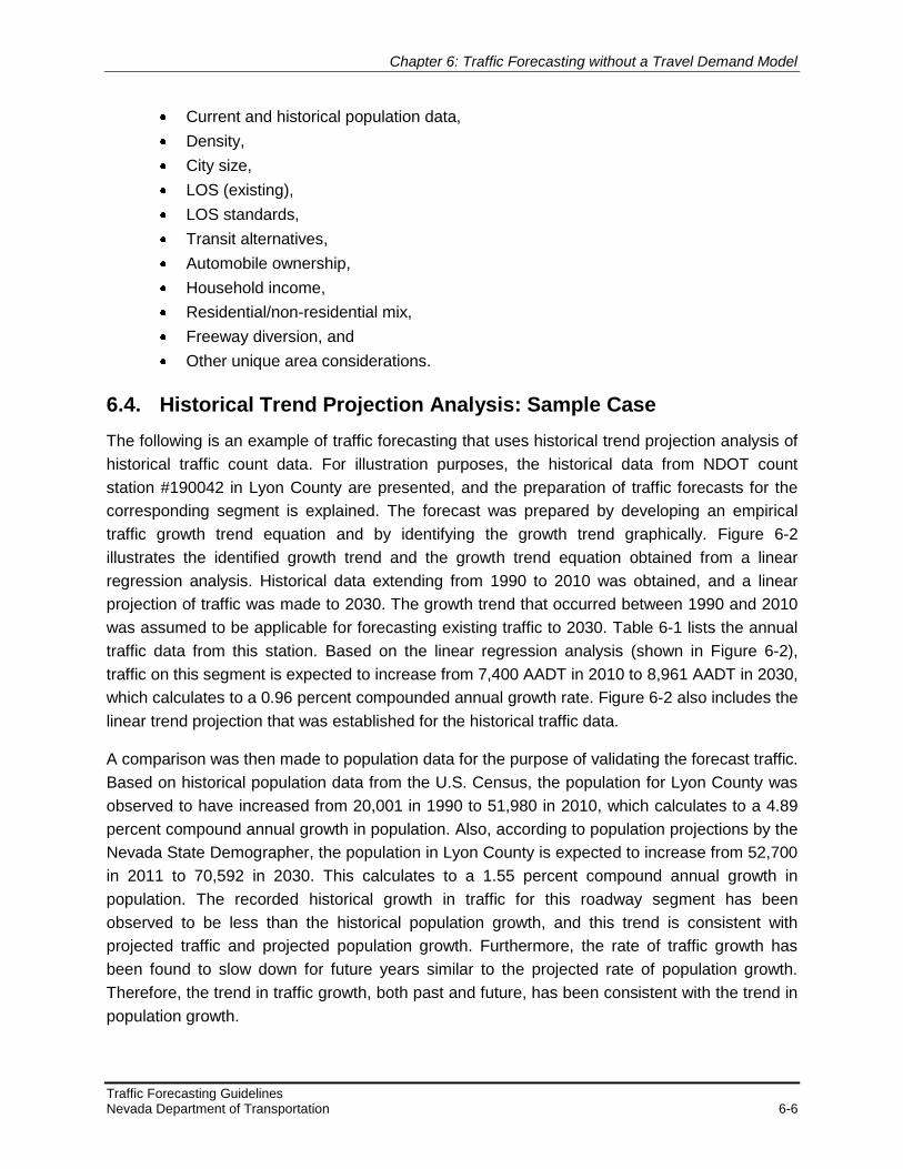
Chapter 6: Traffic Forecasting without a Travel Demand Model
Traffic Forecasting Guidelines Nevada Department of Transportation 6-6
Current and historical population data,
Density,
City size,
LOS (existing),
LOS standards,
Transit alternatives,
Automobile ownership,
Household income,
Residential/non-residential mix,
Freeway diversion, and
Other unique area considerations.
6.4. Historical Trend Projection Analysis: Sample Case
The following is an example of traffic forecasting that uses historical trend projection analysis of
historical traffic count data. For illustration purposes, the historical data from NDOT count
station #190042 in Lyon County are presented, and the preparation of traffic forecasts for the
corresponding segment is explained. The forecast was prepared by developing an empirical
traffic growth trend equation and by identifying the growth trend graphically. Figure 6-2
illustrates the identified growth trend and the growth trend equation obtained from a linear
regression analysis. Historical data extending from 1990 to 2010 was obtained, and a linear
projection of traffic was made to 2030. The growth trend that occurred between 1990 and 2010
was assumed to be applicable for forecasting existing traffic to 2030. Table 6-1 lists the annual
traffic data from this station. Based on the linear regression analysis (shown in Figure 6-2),
traffic on this segment is expected to increase from 7,400 AADT in 2010 to 8,961 AADT in 2030,
which calculates to a 0.96 percent compounded annual growth rate. Figure 6-2 also includes the
linear trend projection that was established for the historical traffic data.
A comparison was then made to population data for the purpose of validating the forecast traffic.
Based on historical population data from the U.S. Census, the population for Lyon County was
observed to have increased from 20,001 in 1990 to 51,980 in 2010, which calculates to a 4.89
percent compound annual growth in population. Also, according to population projections by the
Nevada State Demographer, the population in Lyon County is expected to increase from 52,700
in 2011 to 70,592 in 2030. This calculates to a 1.55 percent compound annual growth in
population. The recorded historical growth in traffic for this roadway segment has been
observed to be less than the historical population growth, and this trend is consistent with
projected traffic and projected population growth. Furthermore, the rate of traffic growth has
been found to slow down for future years similar to the projected rate of population growth.
Therefore, the trend in traffic growth, both past and future, has been consistent with the trend in
population growth.

Chapter 6: Traffic Forecasting without a Travel Demand Model
Traffic Forecasting Guidelines Nevada Department of Transportation 6-7
Table 6-1 Historical AADT for Use in Trend Projection
Year Observed AADT
1990 6,015
1991 5,935
1992 6,840
1993 6,560
1994 6,350
1995 6,685
1996 6,085
1997 6,685
1998 7,380
1999 6,950
2000 6,950
2001 7,090
2002 7,410
2003 7,800
2004 8,000
2005 7,600
2006 7,550
2007 7,400
2008 6,800
2009 6,900
2010 7,400

Chapter 6: Traffic Forecasting without a Travel Demand Model
Traffic Forecasting Guidelines Nevada Department of Transportation 6-8
Linear Trend Projection of AADT
y = 66.331x - 125692
-
3,000
6,000
9,000
12,000
15,000
1990 1995 2000 2005 2010 2015 2020 2025 2030
Year
AA
DT
Figure 6-2 Traffic Growth Trend
Note that a traffic forecast reflects an evaluation of the effect of future traffic growth relative to
historical trends, the addition of major development, the diversion of traffic to nearby roadways,
and the impact of capacity constraints. In all, a traffic forecast is prepared using the best
available resources and engineering judgment.

Chapter 7 Directional Design Hourly Volume Estimates
Traffic Forecasting Guidelines Nevada Department of Transportation 7-1
7. Directional Design Hourly Volume Estimates
DDHV is usually the final metric used for analysis in many projects. This chapter provides the
procedure for arriving at DDHV. In addition, the chapter includes:
A general overview related to LOS operational analysis;
Definition and guidance regarding volume estimates for constrained roadways; and
Additional considerations when drafting the traffic forecast memorandum.
The chapter closes with an overview and sample case of the how to determine peak hours from
DDHV.
7.1. Developing Directional Design Hour Traffic Volumes
As discussed earlier, project specific data are used to derive the K30 and D30 for obtaining DDHV
from AADT. These factors are to be within the ranges established by NDOT from the ATRs (see
Chapter 4 of these Guidelines for a list of the acceptable range of values). In most instances,
there is adequate flexibility within the prescribed range of acceptable values to accommodate
application to individual projects.
Design hour traffic is produced by applying K30 and D30 to AADT projections. The AADT
projections may be the result of the travel demand model generated traffic projections (see
Chapter 5 of these Guidelines), or the projections may be produced by other techniques, such
as historical trend analysis (see Chapter 6 of these Guidelines).
As defined, the K30 converts the 24-hour AADT to an estimate of two-way traffic in the 30th
highest hour of the year, which is required for design purposes and results in DHV. The K30
used for design is to represent unconstrained demand (i.e., it should be obtained from data
measured at a location where the 30th highest hour traffic is not constrained by available
capacity) (see Section 7.3 of these Guidelines for constrained roadways).
Also as discussed previously, D30 converts any DHV two-way traffic volume to an estimated
DDHV. Appropriate D30 values are developed and updated in the same manner described
previously. By convention, the D30 value always pertains to the peak direction of traffic flow
during the design hour. Using both the K30 and D30 values, the estimated DDHV is obtained by
the following equations.
3030 DKAADT)DirectionPeak(DDHV
)D1(KAADT)DirectionPeakOff(DDHV 3030
By applying the above approach, DDHV traffic forecasts are generated for roadway links and
intersection turning movements as needed to satisfy requirements. Turning movement forecasts
are to reflect the logical effects of future year land use and transportation network improvements
on the traffic pattern at a given location. In general, if the pattern of land use and transportation

Chapter 7: Directional Design Hourly Volume Estimates
Traffic Forecasting Guidelines Nevada Department of Transportation 7-2
system characteristics is expected to change, turning movement patterns are also likely to
change over time. Existing turning movements and travel demand model simulation results
(when available) provide useful starting points for the turning movement forecasting process.
The need for turning movement forecast refinements is determined by careful review of the
chosen starting point. The analyst is to use K30, D30, and current turning percentages, if
available, to calculate turning volumes during the design hour.
7.2. LOS Operational Analysis Guidelines
An LOS analysis is to be performed in accordance with the most current HCM procedures. The
HCM procedures are acceptable methods for LOS determination as well as intersection and
roadway lane arrangements. The LOS analysis could include, but is not limited to, intersections,
mainline segments, HOV lanes, ramps, and weaving lanes. HCM software or equivalent
software approved by NDOT may also be used. All LOS analyses, operational, and capacity-
related assessments are to be completed under the direction and supervision of the NDOT
Traffic Operations Division.
Project traffic using design traffic criteria is a forecast of the 30th highest hour traffic volume for
the design year and is required by NDOT for all design projects.
7.3. Definition of a Constrained Roadway
Physical, environmental, or policy constraints may dictate that an existing roadway may not be
expanded even if excess demand for that roadway exists. This type of roadway is called a
constrained roadway. Physical constraints primarily occur when intensive land use development
is immediately adjacent to roadways, thus making expansion costs prohibitive. Environmental
and policy constraints primarily occur when decisions to not expand a roadway are based on
environmental, historical, archaeological, aesthetic, or social impact considerations. Volumes on
constrained roadways are often governed by the capacity of the constrained roadway rather
than K30 and D30 values.
For constrained roadways, the following is also to be considered during the traffic forecasting
process.
If traffic forecasting is carried out with a travel demand model, the travel demand
model would be coded to reflect the constrained number of lanes, and standard
traffic forecasting procedures would apply. Traffic smoothing adjustments are, as
with other travel demand model forecasts, to be reviewed in the development of
model traffic forecasts.
For historical trend projections, procedures outlined in the NCHRP Report 365 are to
be considered. Per the report:
The underlying assumption of the redistribution procedure is that forecast-
year volumes on parallel roadways should tend to be distributed

Chapter 7: Directional Design Hourly Volume Estimates
Traffic Forecasting Guidelines Nevada Department of Transportation 7-3
proportionally to the volumes as observed on the roadways in the base year.
Further stated, if no capacity changes (e.g., widenings and new roadways)
occur between the year observations are made and the forecast year, the
forecast-year volumes on the links intercepted by the screenline are inclined
to be proportional to the base year system. All capacity changes to the
forecast year system are interpreted as new roadways, including widening of
existing roadways (NCHRP 1998).
In other words, the existing capacities are used as guidelines for developing traffic
forecasts. Adjustments are to be made to the distribution for the constrained roadway
in relationship to the impact that the constrained capacity has on the overall existing
distribution capacity and future capacity.
The constrained condition might cause the constrained roadway to exceed accepted
minimum LOS standards. Several iterative steps may be needed prior to finalizing
DHV and DDHV so that project volumes will meet NDOT accepted standards. Use of
standard K30 values are to be reviewed for applicability in converting a constrained
roadway’s AADTs into DHVs and DDHVs. The DHVs and DDHVs may be governed
by the capacity of the constrained roadway rather than the K30 value.
When a desired number of lanes cannot be achieved because of a determination
that the subject roadway is constrained, an analysis is performed to identify whether
an acceptable LOS could be obtained at the constrained roadway by reducing its
traffic load. Methods for achieving such traffic reductions could include the following:
o Improving a parallel roadway,
o Increasing vehicle occupancy,
o Providing transit alternatives,
o Implementing congestion pricing strategies,
o Offering staggered work hour programs, or
o Applying restrictions to future growth.
The congestion reduction strategies may require review of network configuration,
available mode attributes, land use, trip generation, distribution, mode choice, and
assignment components to revise previous system traffic forecasts. After the review,
the DHVs and DDHVs are to be redeveloped.
In the project development phase, it is critical to estimate the year when the
constrained roadway will fail to operate at a desirable LOS. A simple procedure for
obtaining the breakdown year involves obtaining existing and future year DDHV
traffic projections for the constrained roadway. Trend analysis is applied to the data
to obtain intermediate and additional traffic projections. The projected DDHVs are
compared to the minimum LOS volume, and the approximate year of breakdown is
identified (see Figure 7-1). It should be emphasized that actual future year LOS for
an arterial roadway depends on the expected delay at signalized intersections and
overall arterial speed.

Chapter 7: Directional Design Hourly Volume Estimates
Traffic Forecasting Guidelines Nevada Department of Transportation 7-4
Figure 7-1 Constrained Roadway LOS Example Illustrating LOS Breakdown Year
Source: FDOT, Project Traffic Forecasting Handbook 2002
7.4. Determining Peak Hour Design Volumes from DDHV
For many transportation projects in the State, it may be necessary to forecast traffic for multiple
peak hours of traffic of the future years. Most commonly, it may be necessary to forecast traffic
for AM and PM peak hours, but there might also be cases where a midday peak hour sees the
highest traffic volume. As a result, the assignment of the DDHV to an AM, midday or PM peak
hour in the future years is required. To accomplish this, short-term traffic counts and the existing
lane configuration can be examined to determine whether the AM, midday or PM peak hour
during a typical weekday is the critical time period. The DDHV is then applied by convention to
the critical peak hour. For example, if the PM peak hour is found to be the critical time period,
then the DDHV is assigned to the PM peak hour peak direction (e.g., northbound). To determine
the other peak hour peak direction volume, the ratio of the peak direction volumes between the
two peak hours is taken and applied to the DDHV. This ratio of the peak direction volumes
between the two peak hours can be obtained from the typical weekday volumes from the short-
term traffic counts.
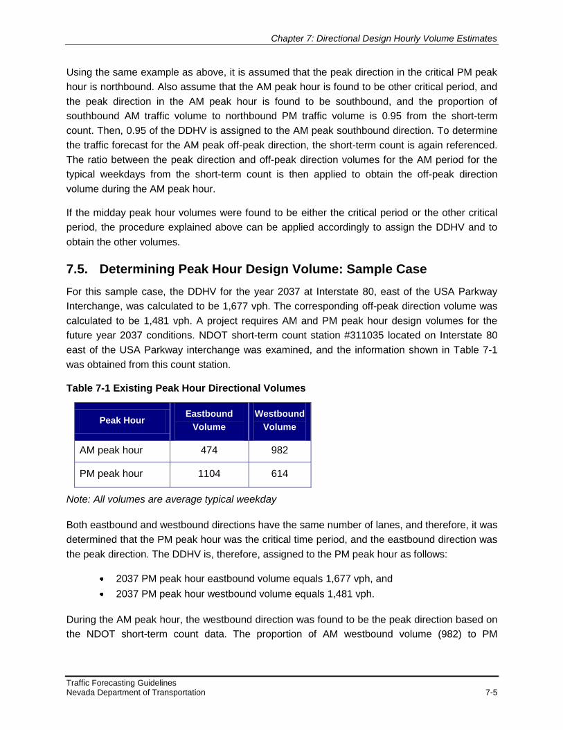
Chapter 7: Directional Design Hourly Volume Estimates
Traffic Forecasting Guidelines Nevada Department of Transportation 7-5
Using the same example as above, it is assumed that the peak direction in the critical PM peak
hour is northbound. Also assume that the AM peak hour is found to be other critical period, and
the peak direction in the AM peak hour is found to be southbound, and the proportion of
southbound AM traffic volume to northbound PM traffic volume is 0.95 from the short-term
count. Then, 0.95 of the DDHV is assigned to the AM peak southbound direction. To determine
the traffic forecast for the AM peak off-peak direction, the short-term count is again referenced.
The ratio between the peak direction and off-peak direction volumes for the AM period for the
typical weekdays from the short-term count is then applied to obtain the off-peak direction
volume during the AM peak hour.
If the midday peak hour volumes were found to be either the critical period or the other critical
period, the procedure explained above can be applied accordingly to assign the DDHV and to
obtain the other volumes.
7.5. Determining Peak Hour Design Volume: Sample Case
For this sample case, the DDHV for the year 2037 at Interstate 80, east of the USA Parkway
Interchange, was calculated to be 1,677 vph. The corresponding off-peak direction volume was
calculated to be 1,481 vph. A project requires AM and PM peak hour design volumes for the
future year 2037 conditions. NDOT short-term count station #311035 located on Interstate 80
east of the USA Parkway interchange was examined, and the information shown in Table 7-1
was obtained from this count station.
Table 7-1 Existing Peak Hour Directional Volumes
Peak Hour Eastbound
Volume
Westbound
Volume
AM peak hour 474 982
PM peak hour 1104 614
Note: All volumes are average typical weekday
Both eastbound and westbound directions have the same number of lanes, and therefore, it was
determined that the PM peak hour was the critical time period, and the eastbound direction was
the peak direction. The DDHV is, therefore, assigned to the PM peak hour as follows:
2037 PM peak hour eastbound volume equals 1,677 vph, and
2037 PM peak hour westbound volume equals 1,481 vph.
During the AM peak hour, the westbound direction was found to be the peak direction based on
the NDOT short-term count data. The proportion of AM westbound volume (982) to PM

Chapter 7: Directional Design Hourly Volume Estimates
Traffic Forecasting Guidelines Nevada Department of Transportation 7-6
eastbound volume (1104) for the typical weekday was calculated from the NDOT short-term
count data using the following equation.
89.0VolumeEastboundPM
VolumeWestboundAM
Therefore, the AM peak hour westbound volume in 2037 is calculated to be 0.89 multiplied by
1,677, which equals 1,493 vph.
For the AM peak hour, the ratio between the peak and off-peak direction volumes (474 and 982)
was calculated for the typical weekdays from the NDOT short-term count data using the
following equation.
48.0VolumeWestboundAM
VolumeEastboundAM
Therefore, the AM peak hour eastbound volume in 2037 is calculated to be 0.48 multiplied by
1,493, which equals 717 vph.
After rounding, the design year 2037 volumes are reported as follows:
PM peak hour eastbound volume equals 1,680 vph;
PM peak hour westbound volume equals 1,480 vph;
AM peak hour westbound volume equals 1,490 vph; and
AM peak hour eastbound volume equals 720 vph.
7.6. Documenting Traffic Forecasts
As noted throughout these Guidelines, when drafting the traffic forecast memorandum, this
guidance presented herein complements what has been listed in the previous chapters. The
draft traffic forecast memorandum is to include all supporting documents used for the traffic
forecasting process, including the documentation of the traffic parameters AADT, K30, D30,
DDHV, and T%.

Chapter 8 Estimating Intersection Turning Movements
Traffic Forecasting Guidelines Nevada Department of Transportation 8-1
8. Estimating Intersection Turning Movements
Intersection turning movements are an essential requirement when conducting an operational
analysis for a project. This chapter provides a methodology for estimating intersection turning
movements and explains techniques for balancing turning movements. The chapter specifies
the recommended tool (Turns W32) in addition to a number of other techniques/tools that can
be used to estimate intersection turning movements.
8.1. Estimating Intersection Turning Movements
Future year estimates of peak hour intersection turning movements are required for intersection
design, traffic operations analysis, and site impact evaluation. Travel demand models, if
available for the study area and if used for the forecasting process, may be able to provide
forecasts of intersection turning movement volumes. However, turning movements obtained
from travel demand models, even after they have been refined for project-level forecasts, may
note erroneous results because of the regional nature of such models. Moreover, it is usually
difficult to generate peak hour volumes directly from a travel demand model for every possible
intersection within a given study area. Travel demand models are also not available in most
rural areas, which would require the analyst to apply other methods to estimate intersection
turning movements. Accordingly, various methods and procedures have been developed to
estimate peak hour turning movement volumes from peak hour traffic volumes. Most of these
methods rely heavily on existing intersection turning movement count data and professional
judgment to estimate future turning movements. While the travel demand models may not
provide accurate turning movement volumes, these turning movement volumes may be an
appropriate starting point in the iterative process to develop acceptable turning movement
volumes.
A review of the methods currently available for use in developing intersection turning
movements indicates that many of the methods can be categorized as “intersection balancing”
methods. Generally speaking, the degree of accuracy that can be obtained from “intersection
balancing” methods depends on the magnitude of incremental change in land use and travel
patterns expected to occur between the base year and future year conditions. These balancing
techniques are used to adjust existing counts as well as travel demand model-generated
counts. The assignment of future turn paths is estimated, and often the departure and arrival
between intersections on the same link will require manual balancing. The algorithms used for
the balancing may not be capable of achieving the desired tolerance. Existing counts need to be
balanced because the turning movements occurring at some driveways may not be included in
traffic counts. The driveways that may not be counted are often commercial strip centers, gas
stations, and other curb cuts that influence the traffic at intersections. The roadway network
coded in the travel demand model generally includes all freeways, arterials, some collectors,
and local roadways. However, some collectors and local roadway that are not coded may be the
key roadways serving the study area. To account for the missing roadways and missing

Chapter 8: Estimating Intersection Turning Movements
Traffic Forecasting Guidelines Nevada Department of Transportation 8-2
driveway information, balancing techniques are used to generate turning movement traffic
volumes.
To date, most algorithms are somewhat interrelated and involve the application of an iterative
procedure that balances future year turning movements based on existing turning movement
counts, approach volumes, and/or turn proportions. These balancing methods can be used for
peak hour volumes, future traffic movements, or any other application that requires balancing
intersection movements.
The following sections offer an overview of some of the techniques used for estimating turning
movements, including the input data required and the relative ease of applying each technique.
The pertinent methods entail the methods described in the NCHRP Report 255, the methods
suggested by H. J. Van Zuylen (1979), and the methods applied by Hauer (1981) and Schaefer
(1988).
8.2. TurnsW32
The TurnsW32 tool is the recommended tool for estimating turning movement volumes in the
State. TurnsW32 was developed by Dowling Associates to compute forecast turning volumes
using the techniques described in NCHRP Report 255. This process is often referred to as the
Furness process of estimating turning movement, which is also how it is referred to in the
program. The subsequent section explains the user interface of the TurnsW32 tool and offers
guidance in applying the tool to estimate turning movements.
8.2.1. TurnsW32 Methodology
TurnsW32 computes forecast turning volumes from existing turning movement volumes and
forecasted future approach and departure volumes. Based upon future trip “ins” and “outs”
(obtained from the travel demand model) along each leg of the intersections, TurnsW32 runs
several iterations to calculate future traffic volumes by turning movement. The iterative
procedure alternately balances the approach flows and departure flows until the results
converge (up to a user-specified maximum number of iterations).
The following steps are involved in using the TurnsW32 program.
Step 1: Enter observed turning volumes, and alternatively enter estimated
percentages of future year’s assigned inflows. If the future estimated percentages
are used, then the totals on each approach must equal 100. (The departure totals will
not equal 100, except by coincidence). When observed turning volumes and
estimated turning percentages are not available, the analyst may enter "1" for the
volume of each permitted movement, this can be used to obtain the turning
movement volumes for intersections along new roadways.

Chapter 8: Estimating Intersection Turning Movements
Traffic Forecasting Guidelines Nevada Department of Transportation 8-3
Step 2: Enter forecast approach and departure volumes. (These volumes may either
be obtained from the travel demand model or from the forecasts made by historical
trend projections.) At any intersection, the inflows must equal the outflows. The
program also offers the analyst an option to “lock in” a predetermined turn volume for
one or more movement. Locking in a turn volume ensures that this volume is
unmodified during the iterative process of estimating turning movements.
The Furness calculation screen of the TurnsW32 program allows the analyst to enter data as
explained below.
8.2.2. TurnsW32 Program Interface
TurnsW32 is a typical Microsoft Windows program with typical user interface options. This
section explains the core menu options of the TurnsW32 program that are concerned with data
input and generating the required outputs. For illustration purposes, data was entered for a
hypothetical intersection (see Figure 8-1, Figure 8-2, and Figure 8-3). The “Manual data entry” is
the basic method that allows the analyst to enter data for each intersection and is discussed
further in these Guidelines. However, for advanced features of the program, the analyst is to
refer to the technical documentation that accompanies the TurnsW32 program. (The following
explanation about the program’s features is adapted from the technical documentation of the
TurnsW32 program.)
The “manual data entry” command is available from the “Options” menu of the program.
Selecting this brings up the “Furness screen” for manual entry of intersection turning movement
volumes as well as approach and departure volumes. The analyst is also presented with options
to name the intersection for which the data is entered (see Figure 8-1).
8.2.2.1. Intersection Data
The upper half of the Furness screen contains the basic intersection information and turning
movement count data used by the program (see Figure 8-2). Intersection numbers are entered
in the blue shaded boxes, and the center box must have a node number because all of the
intersection's information and traffic data are referenced by this number. The other node
numbers, representing the adjacent intersections, are optional. Existing (known) turning
movement counts are entered in the boxes with movement arrows. For "T" intersections, the
analyst is to enter “0” for movements that do not exist. For more accurate results, counted
(rather than estimated) turning movement volumes are to be entered. If counted turning
volumes are not available, enter the estimated turning percentages of the future year's
approach volumes and click on the "Turn %-ages" option button. (If this procedure is used, the
totals on each approach must equal 100, although the departure totals will not equal 100,
except by coincidence). When actual volumes and estimated turning percentages are not
available, the analyst may enter "1" for the volume of each permitted movement and then click
on the "Count data" option button.

Chapter 8: Estimating Intersection Turning Movements
Traffic Forecasting Guidelines Nevada Department of Transportation 8-4
8.2.2.2. Approach/Departure Data
The lower half of the Furness screen provides the option to enter the approach and departure
volumes (see Figure 8-3). Forecast approach and departure volumes are entered in the
unshaded boxes around the outside of the intersection display. The volumes are entered
clockwise starting with the southbound approach volume, then the northbound departure
volume, etc. During the Furness calculation process, if the computed approach and departure
totals are not equal, a balancing dialog box is displayed giving the analyst a choice on the
method to resolve the issue. The methods presented to the analyst are the following.
Balance Manually: The analyst supplies the corrections needed to balance the
entering and leaving totals.
Balance to Highest Total: The lowest total (either approach or departure) will be
factored up to match the highest total.
Balance to Lowest Total: The highest total (either approach or departure) will be
factored down to match the lowest total.
Balance to Average of Entering and Leaving Totals: The approach and departure
volumes will be factored so that their totals both equal the average of the unbalanced
approach and departure totals.
Balance to Entering Total: The departure volumes will be factored so that their total
equals the total approach volumes.
Balance to Leaving Total: The approach volumes will be factored so that their total
equals the total departure volumes.
In most cases, the “Balance Manually” option might provide the best results because the analyst
would be able to apply engineering judgment based on the knowledge of the existing and
expected conditions near the intersections. Hence, the analyst is recommended to balance the
peak hour volumes manually before entering them in TurnsW32.

Chapter 8: Estimating Intersection Turning Movements
Traffic Forecasting Guidelines Nevada Department of Transportation 8-5
Figure 8-1 Manual Data Entry and the Furness Screen

Chapter 8: Estimating Intersection Turning Movements
Traffic Forecasting Guidelines Nevada Department of Transportation 8-6
Figure 8-2 Furness Screen and Iteration Settings

Chapter 8: Estimating Intersection Turning Movements
Traffic Forecasting Guidelines Nevada Department of Transportation 8-7
Figure 8-3 Results Screen
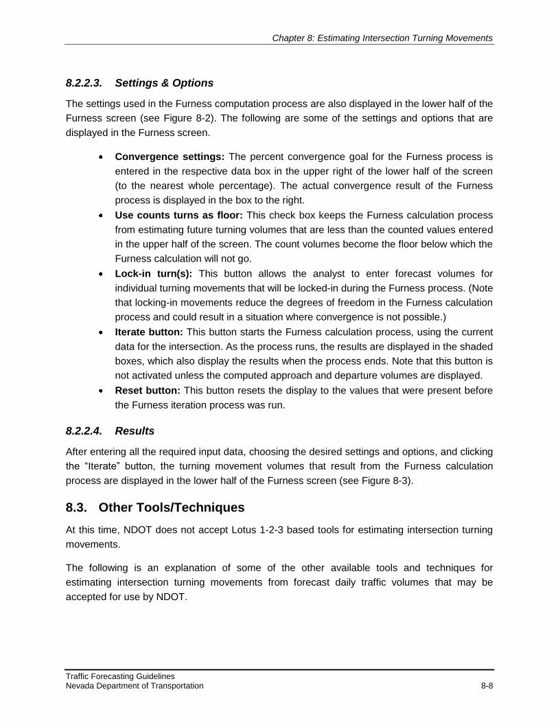
Chapter 8: Estimating Intersection Turning Movements
Traffic Forecasting Guidelines Nevada Department of Transportation 8-8
8.2.2.3. Settings & Options
The settings used in the Furness computation process are also displayed in the lower half of the
Furness screen (see Figure 8-2). The following are some of the settings and options that are
displayed in the Furness screen.
Convergence settings: The percent convergence goal for the Furness process is
entered in the respective data box in the upper right of the lower half of the screen
(to the nearest whole percentage). The actual convergence result of the Furness
process is displayed in the box to the right.
Use counts turns as floor: This check box keeps the Furness calculation process
from estimating future turning volumes that are less than the counted values entered
in the upper half of the screen. The count volumes become the floor below which the
Furness calculation will not go.
Lock-in turn(s): This button allows the analyst to enter forecast volumes for
individual turning movements that will be locked-in during the Furness process. (Note
that locking-in movements reduce the degrees of freedom in the Furness calculation
process and could result in a situation where convergence is not possible.)
Iterate button: This button starts the Furness calculation process, using the current
data for the intersection. As the process runs, the results are displayed in the shaded
boxes, which also display the results when the process ends. Note that this button is
not activated unless the computed approach and departure volumes are displayed.
Reset button: This button resets the display to the values that were present before
the Furness iteration process was run.
8.2.2.4. Results
After entering all the required input data, choosing the desired settings and options, and clicking
the “Iterate” button, the turning movement volumes that result from the Furness calculation
process are displayed in the lower half of the Furness screen (see Figure 8-3).
8.3. Other Tools/Techniques
At this time, NDOT does not accept Lotus 1-2-3 based tools for estimating intersection turning
movements.
The following is an explanation of some of the other available tools and techniques for
estimating intersection turning movements from forecast daily traffic volumes that may be
accepted for use by NDOT.

Chapter 8: Estimating Intersection Turning Movements
Traffic Forecasting Guidelines Nevada Department of Transportation 8-9
8.3.1. TURNS5-V02
The TURNS5-V02 program enables the analyst to obtain turning movements estimates by
operating a Microsoft Excel spreadsheet. The program only requires basic knowledge of
Microsoft Windows and Microsoft Excel. However, the analyst should have a thorough
knowledge of basic traffic engineering principles and be familiar with development of traffic
forecasts by non-automated processes. The use of TURNS5-V02 is acceptable to NDOT for
development of turning movement volumes, and the program has the following characteristics.
Required Input Data
Existing year AADTs
“First guess” turning movement proportions for AADTs
Growth rates to be used or travel demand model year AADTs
K-factor and D-factor
Output Produced
Balanced daily and design hour turning movement forecasts
Existing year, opening year, interim year, and design year forecasts
8.3.2. TMTOOL
The TMTool was developed by FDOT District Four, and it consists of a single Microsoft Excel
spreadsheet with an input, output, and calculations tab. The TMTool may be used for existing
and planned intersections, and the main spreadsheet (TMTOOL.xls) is set up for intersection
turning movement forecasts where detailed information is available. The use of TMTOOL is
acceptable to NDOT for development of turning movement volumes, and tool has the following
characteristics.
Required Input Data
Turning movement distributions
Base year daily approach volumes
Future year growth factors
K-factor and D-factor
Output Data
Balanced AM and PM peak hour turning movement forecasts
Base year and up to three future year forecasts
8.3.3. Manual Method
The manual method consists of a simple calculation technique for obtaining balanced turning
movement volumes from approach volumes at three-legged and four-legged intersections.
Appendix B offers an example of this methodology. Manual methods for development of turning

Chapter 8: Estimating Intersection Turning Movements
Traffic Forecasting Guidelines Nevada Department of Transportation 8-10
movement volumes may be acceptable to NDOT in certain situations, and the method has the
following characteristics.
Required Input Data
Approach volumes
Possibly K-factor and D-factor
Output Data
One set of balanced turning movement forecasts
8.3.4. Growth Factor Technique
To establish future year turning movement forecasts, the growth factor method relies on the
application of projected growth factors to existing year traffic data. The technique has the
following characteristics.
Required Input Data
Existing turning movement counts
Future year growth factors
Possibly K-factor and D-factor
Output Data
Daily and/or peak hour turning movement forecasts
One set of turning movement forecasts
8.3.5. Methods from the NCHRP Report 255
The NCHRP Report 255 suggests three methods for estimating intersection turning movements:
The ratio method,
The difference method, and
The iterative method.
The first two methods assume that relative and absolute differences between the estimated and
observed turn volumes will remain constant over time. Therefore, future turn volumes generated
from models are adjusted according to “ratios” or “differences” calculated from estimated and
observed base year turn movement volumes. The iterative procedure requires base year counts
of intersection approaches. The iterative method employs the traditional Fratar method, which
has been widely used in practice to balance trip tables.
The iterative method is based on an incremental procedure of applying implied growth between
base year and future year to actual traffic counts. Growth rates are derived from the travel
demand model. The iterative procedures would require observed turning movements for all
intersections under study. This method is not applicable to new intersections for which base

Chapter 8: Estimating Intersection Turning Movements
Traffic Forecasting Guidelines Nevada Department of Transportation 8-11
year counts are not available. The Fratar method would produce reasonable results for either
developed areas or areas expected to experience moderate growth in land use. Notably,
TurnsW32 uses the NCHRP Report 255 methods as the basis for developing turning movement
volumes.
8.4. Summary
The differences inherent to each of the described turning movement methods primarily involve
the amount of data input and the information that is generated. These methods could also be
used for areas without a travel demand model (e.g., rural areas) where some information on
existing (and/or historical) travel and expected growth are available. However, estimates would
have to be made for the future approach volumes. Also, existing turning movement data would
have to be used judiciously relative to the expected growth characteristics of the area of the
roadway improvement.
Overall, the TurnsW32 program is the recommended tool for use because of its simplicity and
the available options in the program. At this time, NDOT does not accept Lotus 1-2-3 based
tools for estimating intersection turning movements. As noted throughout, any balancing method
used by the analyst for estimating intersection turning movements are to be documented in the
traffic forecast memorandum, which would include methodology, assumptions, and rationale.

Chapter 9 Truck Traffic Forecasting
Traffic Forecasting Guidelines Nevada Department of Transportation 9-1
9. Truck Traffic Forecasting
This chapter provides the methodology for truck traffic forecasting in instances where historical
truck traffic data is available as well as in instances where data is not available for the project
location. This chapter also explains the process by which to estimate T% and document truck
traffic forecasts.
9.1. Truck Traffic Forecasting Methodology
Estimation of future truck volume is often based on truck traffic history. Several factors can
influence future truck volume, such as land use changes, economic conditions, and new or
competing roadways. Similar to the general trend in traffic growth, truck volume may decrease,
remain constant, or increase, all of which is often illustrated as a straight line, an accelerating
rate (exponential trend), or a decelerating rate (logarithmic trend).
Truck traffic data is collected by means of vehicle classification counts. The purpose of vehicle
classification is to estimate the composition of traffic by vehicle types, and this data can be used
to estimate T%. Vehicle classification data are collected in accordance to the FHWA
Classification Scheme “F” and the 13 vehicle types illustrated on Figure 3-1. When suitable
truck traffic data by class of vehicles is available, truck forecasts are also to be prepared by
each class of vehicles. Similar to the NDOT count stations available for measuring total traffic,
truck volumes are measured by a combination of continuous and short-term classification
stations. Data from the continuous vehicle classification stations are available for current and
previous years where data had been collected. Data from the short-term classification stations
are collected on a three-year cycle, and approximately one-third of the data is available for the
most recent data collection year, with the remaining two-thirds distributed over the previous two
years. Truck AADT values for roadway segments are published by NDOT in their Annual Traffic
Reports.
In general, the amount of historical truck data available from NDOT is not as extensive as the
general traffic data, but this is expected to change in the future. As such, the methodology for
truck traffic forecasting depends on the availability of truck data for the project location. It is
recommended that the analyst contact NDOT’s Traffic Information Division regarding availability
of historical data for the project location.
Figure 9-1 illustrates the truck traffic forecasting methodology.

Chapter 9: Truck Traffic Forecasting
Traffic Forecasting Guidelines Nevada Department of Transportation 9-2
Begin
Is data available for the project location?
Document the forecast and assumptions
Yes No
Perform historical trend projection to estimate future year truck AADT
Is relevant historical
truck traffic data
available?
Use historical data from a location with similar characteristics as that
of the project location. Perform historical trend projection to
estimate future year truck AADT
Estimate current truck percent for the project location. Assume
truck percent to remain stable till the future years or make adjustments as needed
Forecast future year total traffic
Apply truck percent to estimate future year
truck AADT
Yes No
Is current truck traffic data available for a location that is
similar to the expected future
year conditions of the project location?
Obtain truck AADT from the selected location that is similar to
the expected future year conditions of the project location
Use this truck AADT as the forecast truck AADT
for the project
Yes No
Figure 9-1 Truck Traffic Forecasting

Chapter 9: Truck Traffic Forecasting
Traffic Forecasting Guidelines Nevada Department of Transportation 9-3
9.2. Truck Traffic Forecasting Procedures
There are four methods for truck traffic forecasting that can be applied based on the availability
of data and the nature of the project location. The following are to be applied in the order listed
below.
A historical trend projection analysis using historical truck AADT data is the
recommended approach for forecasting future truck traffic when historical truck
AADT data is available for the project location.
If historical truck data is unavailable for the project location, the availability of data for
a location with similar characteristics to that of the project location is to be examined.
If historical data is unavailable for the project location, and a location with similar
characteristics cannot be identified, the analyst is to use current truck traffic data
from a location similar to the expected future year conditions of the project location.
If, after all of these options have been exhausted, suitable truck traffic data is still
unavailable for forecasting, the analyst may apply the “truck traffic as a constant
percentage of total traffic” method.
In all, it is recommended that the analyst apply engineering judgment when forecasting truck
traffic as the extent of historical data available for the regression analysis may be less, resulting
in unreasonable projections. The forecast truck AADT is to be examined for reasonableness
and compared with the change in trend of other quantities, such as population, economic
activity, and transportation demand for commodities.
9.2.1. Truck Traffic Forecasting if Historical Truck AADT Data is Available for
the Project Location
A historical trend projection analysis is conducted if suitable historical truck traffic data is
available for the project location. The procedure of forecasting truck traffic using historical data
is similar to the procedure documented in Chapter 6 of these Guidelines. The historical trend
projection analysis is conducted using the most recent five years of truck AADT data, at a
minimum. But the analysis is to be conducted with as much historical data as possible. The
most commonly used growth trends are linear, logarithmic, and exponential. The use of a
particular trend depends on the historical data and the level of “fit” of a particular trend for the
available historical data.
The steps involved in this process are:
Assembling the data;
Establishing a truck traffic growth trend;
Developing the preliminary truck traffic projection;
Verifying the forecast for reasonableness;

Chapter 9: Truck Traffic Forecasting
Traffic Forecasting Guidelines Nevada Department of Transportation 9-4
Developing a truck traffic forecast in detail;
Conducting a final review and documenting the process.
For a detailed explanation of each step, refer Chapter 6 of these Guidelines.
9.2.2. Truck Traffic Forecasting if Historical Data is Not Available for the
Project Location
If historical truck AADT is not available for the project location, then the next step is to identify
the availability of data for a location that has similar characteristics as that of the project
location. If data is available for a similar location, a historical trend projection is to be conducted
similar to the procedures described in the previous section. The use of historical data from a
different location for forecasting truck traffic must be documented in the methodology
memorandum and the traffic forecast memorandum. NDOT’s consent must be obtained before
proceeding with the forecast.
9.2.3. Truck Traffic Forecasting if Historical Data is Not Available and a
Location with Similar Characteristics Cannot Be Identified
Historical trend projection analysis for a project location may be unfeasible because of a lack of
sufficient historical data. In such a case, the analyst should try to identify locations that have
characteristics similar to the expected future year conditions of the project location. The existing
truck traffic from this similar location can then be used as the future year truck traffic for the
project location. However, the current truck traffic from a chosen location is to be used as future
year truck volumes only if there are strong indicators that the future year project location would
closely resemble the current conditions of the chosen location. For this reason, the analyst is
advised to be extremely cautious when using this method, and all justification and supporting
data when applying the method must be clearly documented in the methodology memorandum
and the traffic forecast memorandum. NDOT’s consent must be obtained before proceeding
with this approach.
9.2.4. Truck Traffic Forecasting if No Suitable Truck AADT Data is Available
If suitable truck traffic data is simply unavailable, the following method may be used to forecast
truck traffic. The method is based on the assumption that the truck traffic remains a constant
percent of the total traffic at a location over the years analyzed. If information regarding the
changing nature of truck traffic is available, adjustments are to be made to the assumed T%.
Step 1: The first step in the estimation of future truck traffic is to identify the truck
percent at the project location for the present day. NDOT’s vehicle classification data
provide the composition of traffic by vehicle types, and these classification counts
may be used to calculate the T%. T% may be calculated for a specific roadway
segment by dividing the truck AADT (if available) by the total AADT for that roadway

Chapter 9: Truck Traffic Forecasting
Traffic Forecasting Guidelines Nevada Department of Transportation 9-5
segment. Truck AADT may be obtained from NDOT’s Annual Vehicle Classification
Report, and the total AADT may be obtained from NDOT’s short-term count stations
or ATRs. NDOT also publishes the typical percent T% for each functional class of
roadway in the State in their annual traffic reports. If the truck AADT is not available
for the project location, this T% reported for the functional class of the roadway can
be used.
Step 2: The second step is to forecast the total traffic at the project location for the
future years (years for which truck forecast is needed). The forecast can either be
made with a travel demand model (see Chapter 5 of these Guidelines) or without a
travel demand model (see Chapter 6 of these Guidelines). If the forecast total traffic
is a quantity other than AADT, this quantity is first to be converted to AADT.
Step 3: Once the future total traffic is available, the third step is to apply the T% to
the forecast traffic to obtain the future year truck traffic.
9.3. Estimating Truck Percent (T%)
As noted, T% is the percentage of truck traffic for 24 hours (one day), and it is calculated as
follows,
AADTTotal
AADTTruck%T
If truck traffic was forecast using the historical trend projection analysis, the result of the
analysis would be the future truck AADT. In this case, T% may be calculated using the above
equation. In contrast, if truck forecasting was done as per the “truck traffic as a constant
percentage of total traffic” method, the T% for the future years is assumed based on the existing
year and is readily available, although adjustments to the assumed T% may be necessary to
account for changing traffic conditions.
9.4. Peak Hour Truck Volumes and Peak Hour Truck Percent
The peak hour truck volume is the volume of truck traffic during the hour of the day that
observes the highest truck traffic volumes. If suitable truck data is available, future peak hour
truck volumes are estimated based on the forecast daily truck volumes and the observed
proportion of daily truck traffic occurring in the peak hour of truck traffic (TP-D). The underlying
assumption here is that the proportion of peak hour truck volumes and daily truck volumes
would remain fairly constant over the years. If information is available regarding the change in
the proportion of peak hour truck volumes to the daily truck volumes, TP-D is to be adjusted
accordingly.
TP-D is to be calculated based on observed truck volumes.

Chapter 9: Truck Traffic Forecasting
Traffic Forecasting Guidelines Nevada Department of Transportation 9-6
volumetruckdailyObserved
volumetruckhourpeakObservedT DP
DPTvolumetruckdailyFuturevolumetruckhourpeakFuture
Once the peak hour truck volumes are obtained, the peak hour truck percent can be calculated
based on the peak hour total volume.
9.5. Documenting Truck Traffic Forecast
The availability of historical data for the project location and the adopted methodology for
forecasting the truck traffic must be clearly documented in the traffic forecast memorandum. Any
assumptions and adjustments made to the forecast must be included, and the rationale behind
these changes must be explained in the traffic forecast memorandum. The relevant forecast
factors, such as the future year truck AADT and T%, must be documented in the traffic forecast
memorandum.

Appendices
Traffic Forecasting Guidelines Nevada Department of Transportation A-1
Appendix A
Appendix A offers guidance for identifying ATRs at locations with characteristics similar to that
of the project location. In addition to NDOT’s functional class assignment of roadways,
classification of the project location could begin by analyzing seasonal traffic trends followed by
area type, number of lanes, weekly traffic trends, and AADT. The subclasses within a number of
these more general classes are listed below.
Based on Seasonal Traffic Trends
Sub Class Description
Interstate Urbanized Stations located on any section of urbanized (areas of
population greater than 50,000) interstate.
Interstate Non-Urbanized Stations located on any section of non-urbanized
interstate.
Commuter
Stations characterized by small seasonal changes in
traffic patterns and commuting between city pairs (also to
be applied to non-State streets in urbanized cities).
Agriculture Stations characterized by late summer and fall harvest
peaks.
Recreational Summer Stations characterized by high summer peaks in
recreational areas.
Recreational Summer/Winter Stations characterized by both summer and winter peaks
in recreational areas.
Recreational Winter Stations characterized by high winter peaks in
recreational areas.
Summer
Stations characterized by a smaller summer increase in
traffic patterns when compared to Recreational Summer
(also to be applied to non-State streets in small cities).
Summer < 2,500 ADT
Stations with less than 2,500 ADT characterized by a
smaller summer increase in traffic patterns when
compared to Recreational Summer (also to be applied for
many rural off-system county roads).
Based on Area Type
Sub Class Description
Urbanized Stations located within areas of population greater than
50,000.

Appendices
Traffic Forecasting Guidelines Nevada Department of Transportation A-2
Based on Area Type
Sub Class Description
Urban Fringe Stations influenced by an urban area, such as an MPO
area.
Small Urban Stations located within areas of population between 5,000
and 49,999.
Small Urban Fringe Stations influenced by a small urban area.
Rural Stations located on routes outside of areas with
population less than 5,000.
Rural Populated
Stations located in cities with a population of less than
5,000 (also to be applied for unincorporated
communities).
Based on Weekly Traffic Trend
Sub Class Description
Weekday Traffic volume trends are greatest on weekdays; typical
for commuter trend and urban areas.
Weekend Traffic volume trends are greatest on weekends; typical
for recreational trend.
Steady Traffic volume trends are steady throughout the week
without significant peaks on the weekend or weekdays.

Appendices
Traffic Forecasting Guidelines Nevada Department of Transportation B-1
Appendix B
Estimating Intersection Turning Movements (an example of the manual method): Appendix B
offers a simple calculation technique for obtaining balanced turning movement volumes from
approach volumes at three-legged and four-legged intersections.

Appendices
Traffic Forecasting Guidelines Nevada Department of Transportation B-2

Appendices
Traffic Forecasting Guidelines Nevada Department of Transportation B-3

Appendices
Traffic Forecasting Guidelines Nevada Department of Transportation B-4