
Traffic Driven Analysis of Cellular Data Networks · 2012-12-05 · Traffic Driven Analysis of...
25
Traffic Driven Analysis of Cellular Data Networks Samir R. Das Computer Science Department Stony Brook University Joint work with Utpal Paul, Luis Ortiz (Stony Brook U), Milind Buddhikot, Anand Prabhu Subramanian (Alcatel‐Lucent Bell Labs)
Transcript of Traffic Driven Analysis of Cellular Data Networks · 2012-12-05 · Traffic Driven Analysis of...
Traffic Driven Analysis of Cellular Data Networks
Samir R. DasComputer Science Department
Stony Brook University
Joint work with Utpal Paul, Luis Ortiz (Stony Brook U), Milind Buddhikot, Anand Prabhu Subramanian (Alcatel‐Lucent Bell Labs)
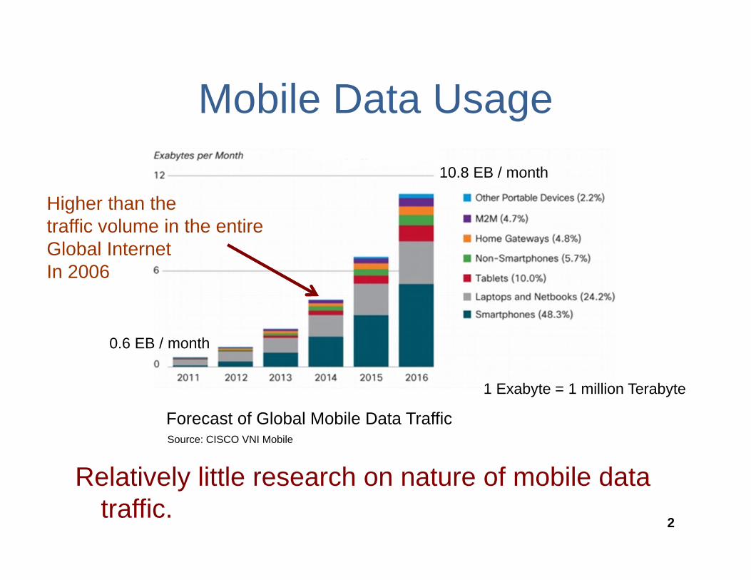
Mobile Data Usage
Relatively little research on nature of mobile data traffic.
2
0.6 EB / month
10.8 EB / month
Forecast of Global Mobile Data TrafficSource: CISCO VNI Mobile
1 Exabyte = 1 million Terabyte
Higher than thetraffic volume in the entire Global Internet In 2006
3
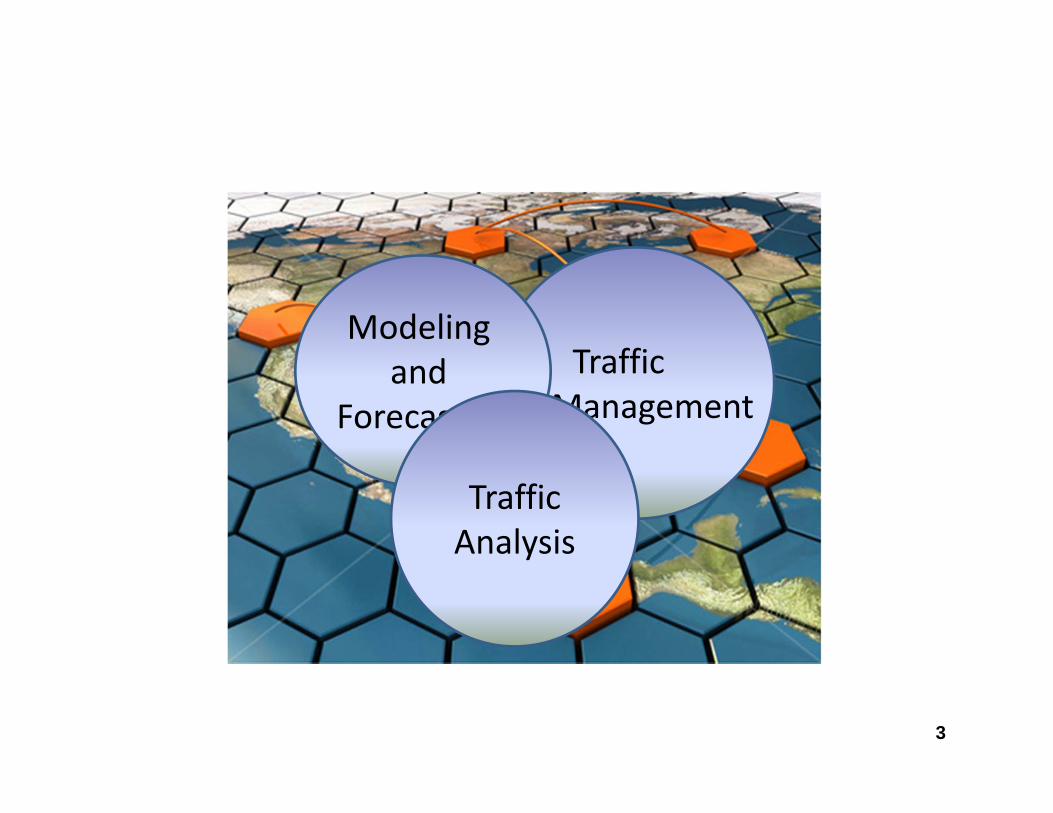
Traffic Management
Modeling and
Forecasting
Traffic Analysis
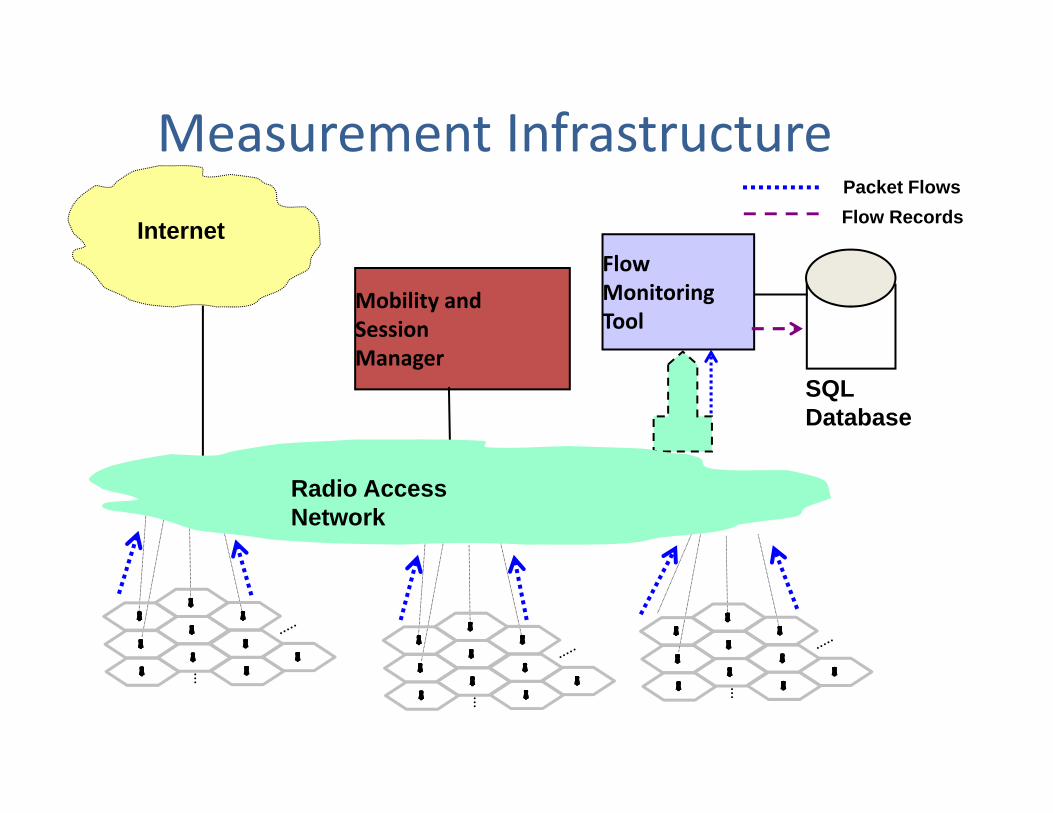
Flow MonitoringTool
SQL Database
Packet Flows
Internet Flow Records
Mobility andSession Manager
Radio AccessNetwork
Measurement Infrastructure
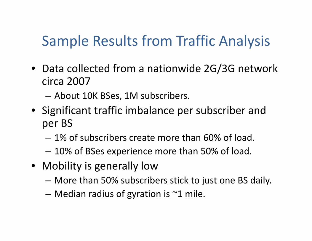
Sample Results from Traffic Analysis
• Data collected from a nationwide 2G/3G network circa 2007– About 10K BSes, 1M subscribers.
• Significant traffic imbalance per subscriber and per BS– 1% of subscribers create more than 60% of load. – 10% of BSes experience more than 50% of load.
• Mobility is generally low– More than 50% subscribers stick to just one BS daily. – Median radius of gyration is ~1 mile.
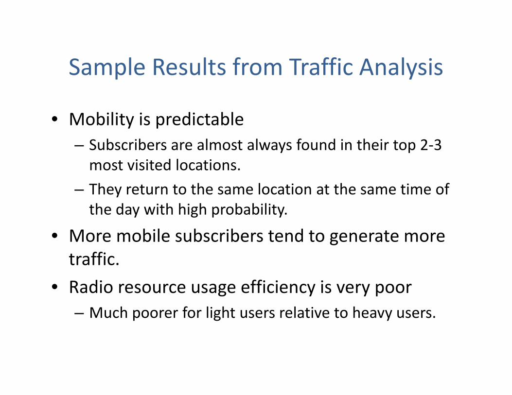
Sample Results from Traffic Analysis
• Mobility is predictable– Subscribers are almost always found in their top 2‐3 most visited locations.
– They return to the same location at the same time of the day with high probability.
• More mobile subscribers tend to generate more traffic.
• Radio resource usage efficiency is very poor– Much poorer for light users relative to heavy users.
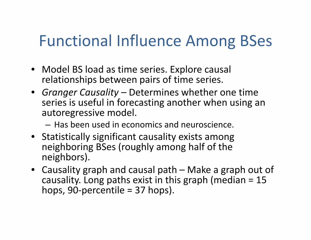
Functional Influence Among BSes• Model BS load as time series. Explore causal relationships between pairs of time series.
• Granger Causality – Determines whether one time series is useful in forecasting another when using an autoregressive model.– Has been used in economics and neuroscience.
• Statistically significant causality exists among neighboring BSes (roughly among half of the neighbors).
• Causality graph and causal path – Make a graph out of causality. Long paths exist in this graph (median = 15 hops, 90‐percentile = 37 hops).
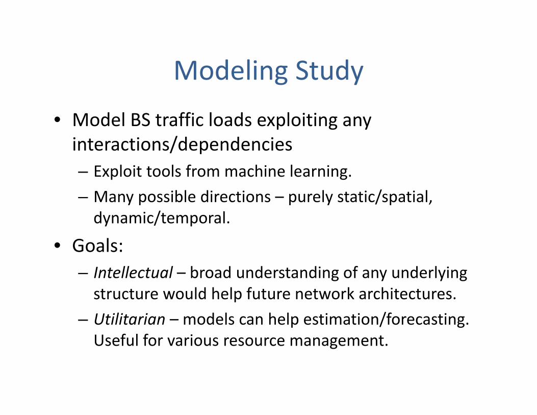
Modeling Study• Model BS traffic loads exploiting any interactions/dependencies– Exploit tools from machine learning. – Many possible directions – purely static/spatial, dynamic/temporal.
• Goals:– Intellectual – broad understanding of any underlying structure would help future network architectures.
– Utilitarian – models can help estimation/forecasting. Useful for various resource management.

• Assume load on n base stations are multi‐variateGaussian:
• Learn the parameters given a set of training data, specifically the “inverse covariance matrix” , given a set of training data (p observations).
• is easier to estimate than and exposes interesting properties.
Spatial Modeling Approach: Probabilistic Graphical Modeling
Mean vector Covariance matrix
1

Inverse Covariance Matrix: Properties
• If then load variables and are conditionally independent, given the rest of the variables.
• Most problems produce a `sparse’ model.
• Related to probabilistic graphical models (e.g., Gaussian Markov Random Field).
12
34
5
Undirected Graphical Model‐> Edge
‐> no edge
Graph properties translate toprobabilistic (in)dependencies
Xi X j
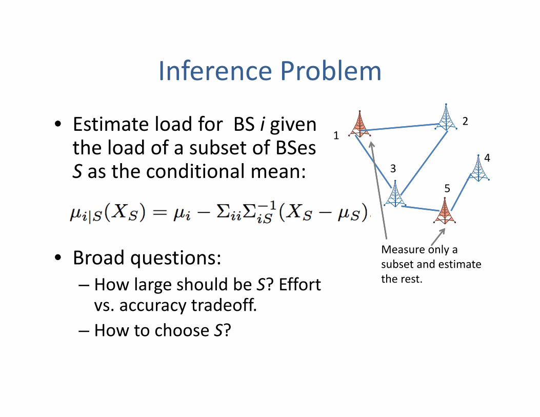
Inference Problem
• Estimate load for BS i given the load of a subset of BSesS as the conditional mean:
• Broad questions: – How large should be S? Effort vs. accuracy tradeoff.
– How to choose S?
12
34
5
Measure only a subset and estimate the rest.
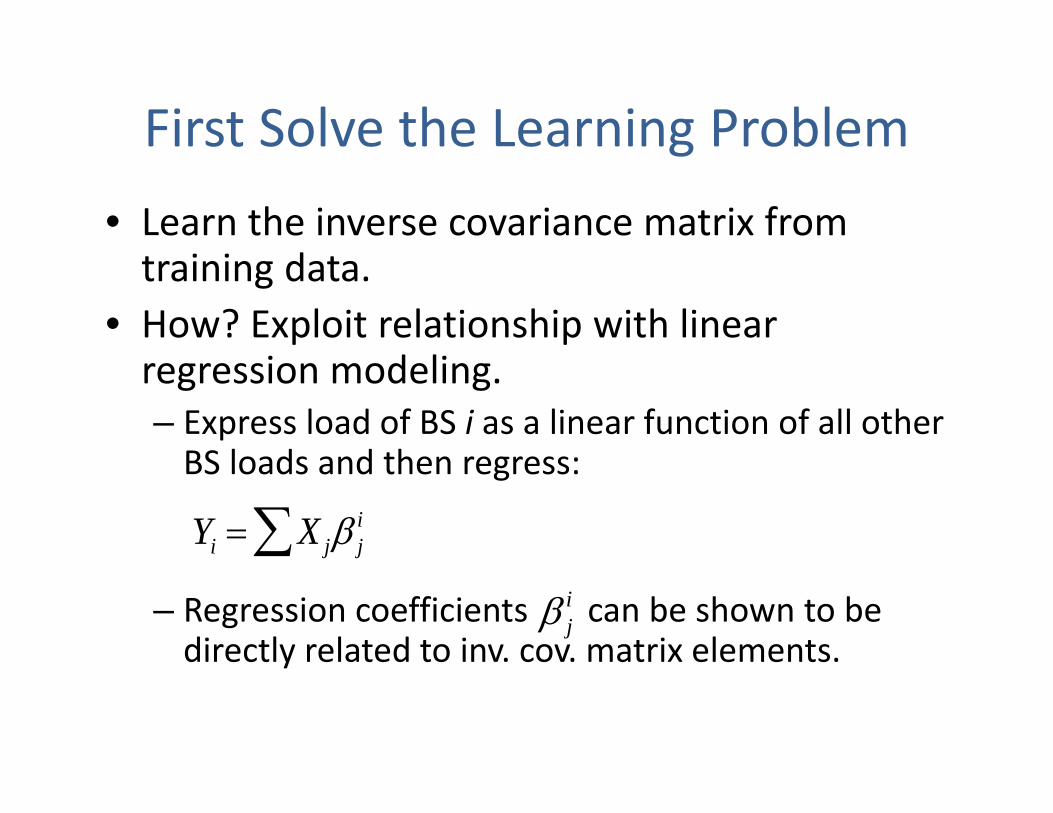
First Solve the Learning Problem• Learn the inverse covariance matrix from training data.
• How? Exploit relationship with linear regression modeling.– Express load of BS i as a linear function of all other BS loads and then regress:
– Regression coefficients can be shown to be directly related to inv. cov. matrix elements.
Yi Xj ji
ji
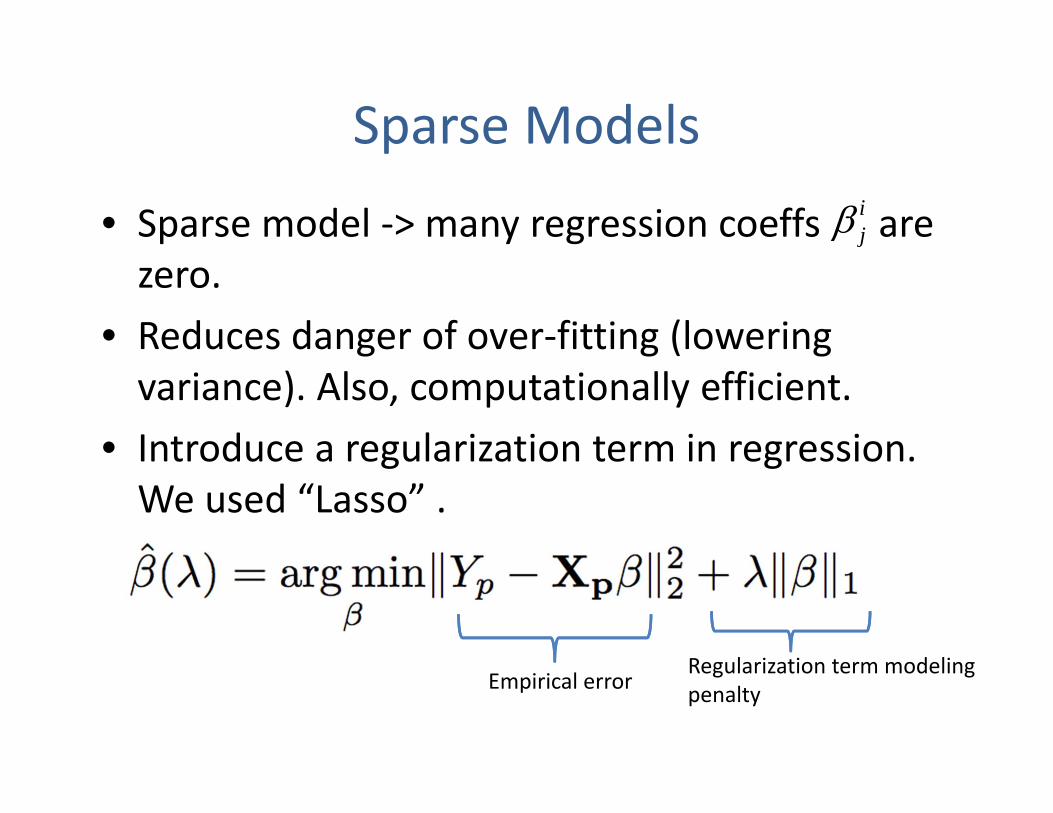
Sparse Models
• Sparse model ‐> many regression coeffs are zero.
• Reduces danger of over‐fitting (lowering variance). Also, computationally efficient.
• Introduce a regularization term in regression. We used “Lasso” .
Empirical errorRegularization term modelingpenalty
ji
Regularization• Cross‐validate using additional training samples (not used for model creation).
• Use various values of to create different models.
• Choose the one with max likelihood.
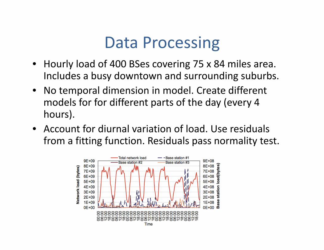
Data Processing• Hourly load of 400 BSes covering 75 x 84 miles area.Includes a busy downtown and surrounding suburbs.
• No temporal dimension in model. Create different models for for different parts of the day (every 4 hours).
• Account for diurnal variation of load. Use residuals from a fitting function. Residuals pass normality test.
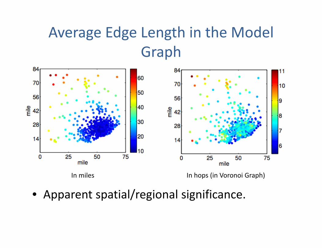
Average Edge Length in the Model Graph
• Apparent spatial/regional significance.
In miles In hops (in Voronoi Graph)
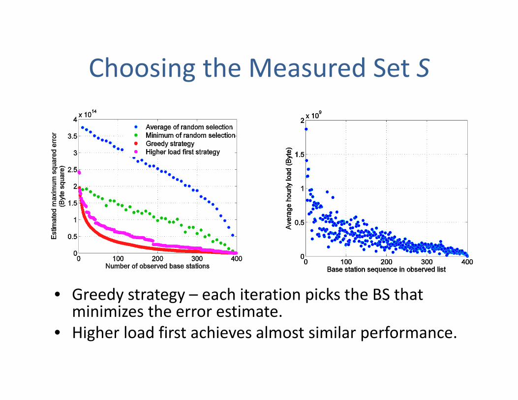
Choosing the Measured Set S
• Greedy strategy – each iteration picks the BS that minimizes the error estimate.
• Higher load first achieves almost similar performance.
Impact of Estimation Accuracy on Applications
• We understand the measurement complexity (size of S) vs. Error tradeoff.
• But how much accuracy do we need? Need to turn to applications
• Studied two applications– Energy Management – Opportunistic Traffic Scheduling
Opportunistic Traffic Scheduling• Similar to Smart Electric Grid – move non‐urgent traffic from peak to off‐peak periods. – What is non‐urgent? p2p, large downloads, sync, push, etc. – Who decides? User agent on mobile. May have multiple levels of priority or have deadlines to aid scheduling.
– Carriers can incentivize such scheduling. • Similar to QoS scheduling – but at a higher layer and at a longer time scale.
• Two components in System Architecture– Server (Scheduler) in core network.– User agent on mobile that coordinates with Server.
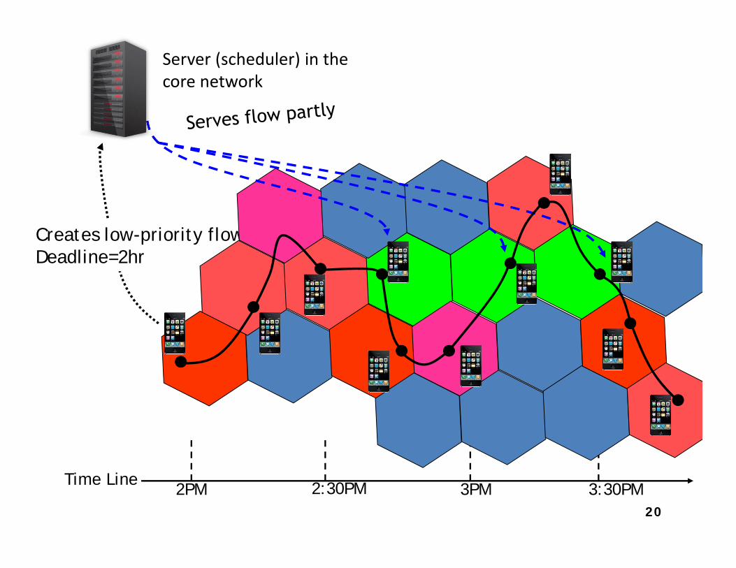
Time Line2PM 2:30PM 3PM 3:30PM
Creates low-priority flow Deadline=2hr
20
Server (scheduler) in the core network
Solving the Scheduling Problem• Several approaches possible based on how flows are prioritized.
• But for any approach, server needs to be able estimate current/future loads at all BSes. – Also, needs to model/estimate subscriber mobility (separate problem).
• Poor estimation leads to poor scheduler performance.
Evaluation Approach• Trace‐driven simulator based on a capacity model of BSes.
• Opportunistic scheduling is meant to admit more traffic but with the same network capacity.
• We use the same traffic trace always, but reduce network capacity to demonstrate impact.
• Impact?– Do low priority flows still finish within a reasonable time?
– Are high priority flows impacted?
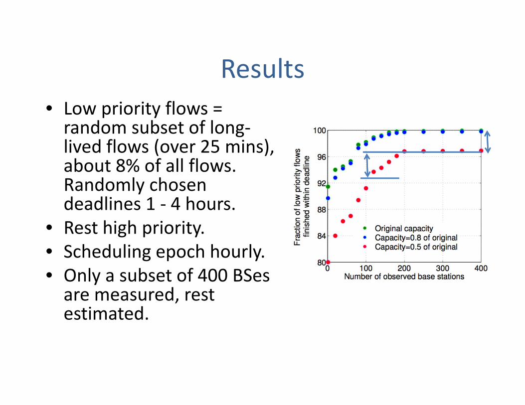
Results• Low priority flows = random subset of long‐lived flows (over 25 mins), about 8% of all flows. Randomly chosen deadlines 1 ‐ 4 hours.
• Rest high priority. • Scheduling epoch hourly. • Only a subset of 400 BSesare measured, rest estimated.
Conclusions
• Discovering structures in mobile traffic is a rich area of study.
• Applications in network and resource management.
25
Traffic Management
Modeling and
Forecasting
Traffic Analysis
Questions?