SlideshareData management implications of the Fundamental Review of the Trading Book (FRTB)

THE JOURNAL OF FINANCE • VOL. LXI, NO. 6 • DECEMBER 2006
Trading Volume: Implications of anIntertemporal Capital Asset Pricing Model
ANDREW W. LO and JIANG WANG∗
ABSTRACT
We derive an intertemporal asset pricing model and explore its implications for trading
volume and asset returns. We show that investors trade in only two portfolios: the
market portfolio, and a hedging portfolio that is used to hedge the risk of changing
market conditions. We empirically identify the hedging portfolio using weekly volume
and returns data for U.S. stocks, and then test two of its properties implied by the
theory: Its return should be an additional risk factor in explaining the cross section
of asset returns, and should also be the best predictor of future market returns.
FUNDAMENTAL SHOCKS TO THE ECONOMY DRIVE BOTH THE SUPPLY and demand of finan-cial assets and their prices. Therefore, any asset pricing model that attemptsto establish a structural link between asset prices and underlying economicfactors also establishes links between prices and quantities such as tradingvolume since economic fundamentals such as the investors’ preferences andthe assets’ future payoffs determine the joint behavior of prices and quanti-ties.1 The construction and empirical implementation of any asset pricing modelshould therefore involve both price and quantity as key elements. Indeed, froma purely empirical perspective, the joint behavior of price and quantity revealsmore information about the relation between asset prices and economic factorsthan do prices alone. The asset pricing literature, however, has focused moreon prices and much less on quantities. For example, empirical investigationsof well known asset pricing models such as the Capital Asset Pricing Model(CAPM) and its intertemporal (ICAPM) extensions focus exclusively on pricesand returns, completely ignoring the information contained in quantities. In
∗Lo is from MIT Sloan School of Management, and National Bureau of Economic Research
(NBER), and Wang is from MIT Sloan School of Management, NBER, and China Center for
Financial Research. The authors thank Joon Chae, Ilan Guedj, Jannette Papastaikoudi, Antti
Petajisto, and Jean-Paul Sursock for excellent research assistance, and Jonathan Lewellen for pro-
viding his industry classification scheme. They are grateful to Wayne Ferson and seminar and
conference participants at Boston College, the Chinese University of Hong Kong, Duke University,
Georgetown University, Harvard Business School, London Business School, New York University,
Oxford University, the Shenzhen Stock Exchange, UCLA, University of North Carolina, Univer-
sity of Pennsylvania, University of Toronto, the 8th World Congress of the Econometric Society,
the 2001 Lectures in Financial Economics in Beijing and Taipei, the 2005 CORE Lectures at the
Universite Catholique de Louvain for helpful comments and suggestions. Financial support from
the MIT Laboratory for Financial Engineering and the National Science Foundation (Grant No.
SBR–9709976) is gratefully acknowledged.1 See, for example, Campbell, Grossman, and Wang (1993) and Wang (1994).
2805

2806 The Journal of Finance
this paper, we hope to show that even if our main interest is the behavior ofprices, valuable information about price dynamics can be extracted from trad-ing volume.
We begin by developing an intertemporal capital asset pricing model of multi-ple assets in the spirit of Merton’s ICAPM (Merton, 1973). In our model, assetsare exposed to market risk and the risk of changes in market conditions.2 As aresult, investors wish to hold two distinct portfolios of risky assets, namely, themarket portfolio and a hedging portfolio. The market portfolio allows investorsto adjust their exposure to market risk, and the hedging portfolio allows themto hedge the risk of changes in market conditions. In equilibrium, a two-factorlinear pricing model holds, where the two factors are the returns on the marketportfolio and the hedging portfolio, respectively.
We then explore the implications of this model on the joint behavior of vol-ume and returns. Since investors hold only two portfolios, trading volume alsoexhibits a two-factor structure. The first factor arises from trades in the marketportfolio and the second from trades in the hedging portfolio. More importantly,the factor loading of each asset’s trading volume on the hedging portfolio factoris proportional to that asset’s portfolio weight in the hedging portfolio. Thisremarkable property of the trading volume of individual assets suggests a wayto identify the hedging portfolio from a rather unexpected source: volume data.
Using weekly returns and trading volume for NYSE and AMEX stocks from1962 to 2004, we implement the model empirically. From the trading volume ofindividual stocks, we construct the hedging portfolio and its returns. We findthat the hedging portfolio return consistently outperforms other predictors inforecasting future returns to the market portfolio. We then use the returns tothe hedging and market portfolios as two risk-factors in a cross-sectional testalong the lines of Fama and MacBeth (1973), and find that the hedging port-folio is comparable to other factors in explaining the cross-sectional variationof expected returns. Collectively, these results provide concrete economic foun-dations for determining risk factors beyond the market portfolio for dynamicequilibrium asset pricing models.
In Section I, we present our intertemporal equilibrium model of asset-pricingand trading volume. In Section II, we explore the model’s implications for vol-ume and returns. Section III contains a description of the data used in ourempirical implementation of the model, as well as an outline of the construc-tion of the hedging portfolio. In Section IV, we compare the forecast power ofthe hedging portfolio with other factors, and we perform cross-sectional tests ofthe hedging portfolio as a risk factor in Section V. We conclude in Section VI.
I. The Model
In this section, we develop an intertemporal equilibrium asset pricing modelwith multiple assets and heterogeneous investors. Since our purpose is to derive
2 One example of changes in market conditions is that of changes in the investment opportunity
set considered by Merton (1971, 1973).
Trading Volume 2807
qualitative implications for the joint behavior of return and volume, the modelin subsection A is kept as parsimonious as possible. We discuss several gener-alizations of the model in subsection B.
A. The Economy
We consider an economy defined on a set of discrete dates t = 0, 1, 2, . . . . Thereare J risky assets, or “stocks, ” in the economy. Let Djt denote the date t dividendfor each share of stock j, j = 1, . . . , J, and Dt ≡ (D1t; . . . ; DJt) denote the columnvector of dividends.3 Without loss of generality, we normalize the number ofshares outstanding for each stock to be one.
A stock portfolio can be expressed in terms of its shares of each stock, denotedby S ≡ (S1; . . . ; SJ), where Sj is the number of stock-j shares in the portfolio( j = 1, . . . , J ). A portfolio of particular importance is the market portfolio, de-noted by SM, which is given by
SM = (1; . . . ; 1) (1)
under our normalization. The dividend on the market portfolio is then given byDMt ≡ S′
MDt, which is the aggregate dividend.In addition to stocks, there is also a risk-free bond that yields a constant,
positive rate of interest, r, per time period.There are I investors in the economy, each endowed with equal shares of
the stocks and no bonds. Every period, investor i, i = 1, . . . , I, maximizes hisexpected utility of the following form:
Et
[−e−W i
t+1−(λX X t+λY Y i
t
)DMt+1−λZ
(1+Z i
t
)X t+1
], (2)
where Wit+1 is investor i’s next-period wealth, Xt, Yi
t , and Zit are three one-
dimensional state variables, and λX , λY , and λZ are nonnegative constants. Theutility function specified in (2) is state-dependent.4 We further assume
I∑i=1
Y it =
I∑i=1
Z it = 0, (3)
where t = 0, 1, . . . .
3 Throughout this paper, we adopt the following convention: For a set of elements
e1, . . . , en, (e1; . . . ; en) denotes the column vector and (e1, . . . , en) denotes the row vector from these
elements.4 Using a multiasset extension of the setting in Wang (1994)—which is similar to our setting
here except that, in addition to traded assets, investors also hold nontraded assets whose payoffs
are driven by exogenous state variables, denoted by Xt and Yit—we can show that the resulting
value function takes the form that is qualitatively identical to the utility function given in (2). For
brevity, we directly assume the form of the (indirect) utility function here because our purpose is
to capture the trading behavior of investors under the given risk structure.
2808 The Journal of Finance
For simplicity, we assume that all the exogenous shocks—Dt, Xt, {Yit , Zi
t, i =1, . . . , I }—are independently and identically distributed (I.I.D.) over time withzero means. For tractability, we further assume that Dt and Xt are jointly nor-mally distributed:
ut ≡(
Dt
X t
)d∼ N (·, σ ) , where σ =
(σDD σDX
σX D σX X
). (4)
Without loss of generality, σDD is assumed to be positive definite.
B. Discussion
Our model has several features that might seem unusual. Most importantly,the specification in (2) assumes investors have a myopic but state-dependentutility function. We use this utility function to capture the dynamic nature ofthe investment problem without having to explicitly solve a dynamic optimiza-tion problem. This utility function should be interpreted as the equivalent of avalue function from an appropriately specified dynamic optimization problem(see, e.g., Wang (1994) and Lo and Wang (2003)). In particular, it is possible tospecify a canonical dynamic optimization problem for investors in which theyhave state-independent utility over their lifetime consumption such that theresulting value function—a function of wealth and the state variables—has aform similar to the state-dependent utility function in (2).5 Therefore, for expo-sitional simplicity, we start with (2).
The state dependence of the utility function has the following properties. Themarginal utility of wealth depends on the dividend of the market portfolio (theaggregate dividend), as reflected in the second term in the exponential ofthe utility function. When the aggregate dividend increases, the marginal util-ity of wealth declines. There are many ways to motivate this type of utilityfunction. For example, utility can be derived from wealth relative to the mar-ket, rather than the level of wealth itself (see, e.g., Abel (1990), Campbelland Cochrane (1999)). Alternatively, in addition to their stock investments,investors can be exposed to other risks that are correlated with the market(see, e.g., Wang (1994)). The marginal utility of wealth also depends on fu-ture state variables, and in particular Xt+1, as reflected in the third term inthe exponential of the utility function. The motivation for allowing such de-pendence is as follows. Since the state variables determine stock returns inequilibrium, the value function (or indirect utility function) of an investor whooptimizes dynamically would depend on these state variables. Without model-ing the dynamic optimization problem explicitly, we impose such dependenceon the (myopic) utility function. This dependence introduces dynamic hedgingmotives in investors’ portfolio choices (see Merton (1971) for a discussion ofdynamic hedging).
5 As Wang (1994) shows, under CARA and time-separable preferences over lifetime consumption
and Gaussian processes for asset returns and income, an investor’s value function has a similar
form to (2).

Trading Volume 2809
Another simplification in the model is the I.I.D. assumption for the statevariables. This might leave the impression that the model is effectively static.However, this is not the case since the state-dependence of the utility functionintroduces important dynamics over time, allowing for richer state-variabledynamics in particular without changing the main properties of the model.
The particular form of the utility function and normality of the state variablesare assumed for tractability, and such assumptions are restrictive. We hope thatthe qualitative predictions of our model are not sensitive to these assumptions.
We also assume an exogenous interest rate for the bond, and do not requirethe bond market to clear. This modeling choice allows us to simplify our analysisand focus squarely on the stock market. It will become clear later that changesin the interest rate are not important for the issues we consider in this paper.Moreover, from an empirical point of view, at the frequency of interest here(weekly), changes in interest rates are usually small.
C. Equilibrium
Let Pt ≡ (P1t; . . . ; PJt) and Sit ≡ (Si
1t; . . . ; SiJt) be the column vectors of ex-
dividend stock prices and investor i’s stock holdings, respectively. We now derivethe equilibrium of the economy.
DEFINITION 1: An equilibrium is given by a price process {Pt : t = 0, 1, . . . } andthe investors’ stock positions {Si
t : i = 1, . . . , I; t = 0, 1, . . . } such that:
1. Sit solves investor i’s optimization problem
Sit = arg max E
[−e−W i
t+1−(λX X t+λY Y i
t
)DMt+1−λZ
(1+Z i
t
)X t+1
](5)
s. t. W it+1 = W i
t + Si′t [Dt+1 + Pt+1 − (1+r)Pt]. (6)
2. The stock market clears:
i∑i=1
Sit = SM . (7)
This definition of equilibrium is standard except that here the bond marketdoes not clear. As we discussed earlier, the interest rate is given exogenouslyand there is an infinitely elastic supply of bonds at that rate.
For t = 0, 1, . . . , let Qt+1 denote the vector of excess dollar returns on thestock, that is,
Qt+1 ≡ Dt+1 + Pt+1 − (1+r)Pt . (8)
Thus, Qjt+1 = Djt+1 + Pjt+1 − (1 + r)Pjt gives the dollar return on one share ofstock j in excess of its financing cost for period t + 1. For the remainder ofthe paper, we simply refer to Qjt+1 as the dollar return of stock j, omittingthe qualifier “excess.” The dollar return Qjt+1 differs from the conventional

2810 The Journal of Finance
return measure Rjt+1, which is the dollar return normalized by the share price:Rjt+1 ≡ Qjt+1/Pjt. We refer to Rjt+1 simply as the return on stock j in periodt + 1.
We can now state the solution to the equilibrium in the following theorem:
THEOREM 1: The economy defined above has a unique linear equilibrium inwhich
Pt = − a − bX t (9)
and
Sit = (
1/I − λY Y it
)SM − [
λY (b′ι)Y it + λZ Z i
t
](σQQ)−1σQX , (10)
where ι is a vector of ones,
σQQ = σDD − (bσXD + σDXb′) + σ 2X bb′, (11a)
σQX = σDX − σ 2X b, (11b)
a = 1
r
(ασQQSM + λZ σQX
), (11c)
b = λX[(1 + r) + (λZ σXDSM )
]−1σDDSM , (11d)
and α = 1/I .
The nature of the equilibrium is intuitive. In our model, an investor’s utilityfunction depends not only on his wealth, but also on the stock payoffs directly. Inother words, even if he holds no stocks, his utility fluctuates with the stocks’ pay-offs. Such “market spirits ”—as opposed to “animal spirits ”—affect his demandfor stocks, in addition to the usual factors such as the stocks’ expected returns.We measure the market spirits of investor i by (λXXt + λYYi
t ). If (λXXt + λZYit )
is positive, investor i extracts positive utility when the aggregate stock payoffis high. Such a positive “attachment ” to the market makes holding stocks lessattractive to him. If (λXXt + λYYi
t ) is negative, he has a negative attachmentto the market, which makes holding stocks more attractive. At the aggregatelevel, such market spirits, which are captured by Xt, affect aggregate stock de-mand, which in turn affect equilibrium stock prices. Given the particular formof the utility function, Xt affects equilibrium stock prices linearly. In contrast,idiosyncratic differences among investors in the magnitudes of their marketspirits, which are captured by Yi
t , offset each other at the aggregate level, andthus they do not affect equilibrium stock prices. However, they do affect indi-vidual investors’ stock holdings. As the first term of (10) shows, investors withpositive Yi
ts hold less stocks (that is, they gain utility by merely observing stockpayoffs).
Since the aggregate utility variable Xt drives stock prices, it also drives stockreturns. In fact, the expected return of stocks changes with Xt (see the discussion

Trading Volume 2811
in the next section). The form of the utility function also implies that the in-vestors’ utility functions depend directly on Xt, which fully characterizes themarket conditions that investors face, that is, the investment opportunities.Such a dependence arises endogenously when investors optimize dynamically.In our setting, however, we assume that investors optimize myopically, so weinsert such a dependence directly into the utility function. This dependenceinduces investors to care about future market conditions when choosing theirportfolios. In particular, they prefer those portfolios whose returns can helpthem to smooth fluctuations in their utility that are due to changes in marketconditions. Such a preference gives rise to the hedging component in their assetdemand, which is captured by the second term in (10).
II. The Behavior of Returns and Volume
Given the intertemporal CAPM defined above, we can derive its implicationsfor the behavior of returns and volume. For stocks, their dollar return vectorcan be reexpressed as
Qt+1 = ra + (1 + r)bXt + Q t+1, (12)
where Q t+1 ≡ Dt+1 − bX t+1 denotes the vector of unexpected dollar returns onthe stocks, which are I.I.D. over time with zero mean. Equation (12) shows thatthe expected returns on stocks change over time. In particular, they are drivenby a single state variable, Xt.
The investors’ stock holdings can be expressed in the following form:
Sit = hi
MtSM + hiHtSH ∀ i = 1, 2, . . . , I , (13)
where hiMt ≡ (1/I ) − λYYi
t , hiHt ≡ λY (b′SM)Yi
t − λZZit, and
SH ≡ (σQ Q
)−1σQ X . (14)
Equation (13) states that two-fund separation holds for the investors’ stockinvestments. That is, the stock investments of all investors can be viewed asinvestments in two common funds: the market portfolio SM and the hedgingportfolio SH.6 In our model, these two portfolios, expressed in terms of stockshares, are constant over time.
The particular structure of the returns and the investors’ portfolios lead toseveral interesting predictions about the behavior of volume and returns, whichwe summarize in Propositions 1–4.
6 Note that the investors’ total portfolios satisfy three-fund monetary separation—the risk-free
bond and the two stock funds. For our discussion here, we restrict our attention to investors’ stock
investments and always focus on the two stock funds.

2812 The Journal of Finance
A. The Cross-Section of Volume
Given heterogeneity in preferences, which change over time, investors tradeamong themselves to achieve their optimal stock holdings. The volume of tradecan be measured by the turnover ratio (see Lo and Wang (2000)). Since wenormalize the total number of shares outstanding to be one for all stocks, theturnover of a stock, say, stock j, is given by
τ j t ≡ 1
2
I∑i=1
∣∣ (hiMt − hi
Mt−1
)+
(hi
Ht − hiHt−1
)SH j
∣∣, ∀ j = 1, . . . , J . (15)
Let τ t denote the vector of turnover for all stocks. We have the following propo-sition for the cross-section of volume:
PROPOSITION 1: When trading in the hedging portfolio is small relative to tradingin the market portfolio,7 the two-fund separation in investors’ stock holdingsleads to a two-factor structure for stock turnover
τt ≈ SM FMt + SH FHt, (16)
where
FMt = 1
2
I∑i=1
∣∣hiMt − hi
Mt−1
∣∣ and FHt = 1
2
I∑i=1
(hi
Ht − hiHt−1
)Sign
(hi
Mt − hiMt−1
).
(17)
In the special case where one-fund separation holds for stock holdings (whenXt = 0, ∀ t), turnover has an exact one-factor structure, τt = SMFMt. Moreover,the loadings of individual turnover on the common factor are identical acrossall stocks, hence turnover is identical across all stocks. This is not surprising—in the case of one-fund separation for stock investments, investors trade in onestock portfolio, which has to be the market portfolio, and thus they must tradeall the stocks in the same proportions (in shares). Consequently, the turnovermust be the same for all stocks.8
In the general case where two-fund separation holds for stock investments,and assuming that the trading in the market portfolio dominates the tradingin the hedging portfolio, turnover has a two-factor structure (after a linear ap-proximation) as given in (16). Although parameter restrictions can be imposedin the theoretical model to satisfy the condition that trading in the hedgingportfolio be small (see the Appendix), it is an empirical question as to whetherthis and the two-factor model are plausible, which we address in the empiricalanalysis of Section III.
It is important to note that the loading of stock j’s turnover on the secondfactor is proportional to its share weight in the hedging portfolio. Therefore,
7 This imposes certain restrictions on the λ coefficients and the other model parameters. See the
proof in the Appendix for more details.8 For a discussion on the implications of mutual fund separation on the cross-sectional behavior
of volume, see Lo and Wang (2000). See also Tkac (1996).

Trading Volume 2813
if we can empirically identify the two common factors FMt and FHt, the stocks’loadings on the second factor will allow us to identify the hedging portfolio.In our empirical analysis, we explore the information that the cross sectionof volume contains. As we discuss below, the hedging portfolio has importantproperties that allow us to better understand the behavior of returns. Merton(1971, 1973) considers the properties of hedging portfolios in a continuous-timeframework as a characterization of equilibrium. Our discussion here followsMerton in spirit, but is set in a discrete-time, equilibrium environment.
B. Time Series Implications for the Hedging Portfolio
By the definition of the hedging portfolio in (14), it is easy to show that itscurrent return gives the best forecast of future market returns.
Let QMt+1 denote the dollar return on the market portfolio in period t + 1,and QHt+1 denote the dollar return on the hedging portfolio. Then,
Q Mt+1 = S′M Qt+1 and Q Ht+1 = S′
H Qt+1. (18)
For an arbitrary portfolio S, its dollar return in period t, which is QSt ≡ S′Qt,can serve as a predictor for the next-period dollar return of the market:
Q Mt+1 = δ0 + δ1 QSt + εMt+1. (19)
The predictive power of S is measured by the R2 of the above regression. Wecan solve for the portfolio that maximizes the R2. The solution, up to a scalingconstant, is the hedging portfolio. Thus, we have the following result:
PROPOSITION 2: Among the returns of all portfolios, the dollar return of the hedg-ing portfolio, SH, provides the best forecast for the future dollar return of themarket.
In other words, if we regress the market dollar return on the lagged dollar-return of any set of portfolios, the hedging portfolio must yield the highest R2.
C. Cross-Sectional Implications for the Hedging Portfolio
We now turn to the predictions of our model for the cross section of re-turns. Let Qp t+1 denote the dollar return of a stock portfolio, Q p t+1 ≡ Et[Q p t+1]
its conditional expectation at time t, Q p its unconditional expectation, and
Q p t+1 ≡ Q p t+1 − Q p t+1 its unexpected dollar return in period t + 1. Then,
Q Mt+1 and Q Ht+1 denote the unexpected dollar returns on the market port-folio and the hedging portfolio, respectively, and
σ 2M ≡ Var[Q Mt+1], σ 2
H ≡ Var[Q Ht+1], and σMH ≡ Cov[Q Mt+1, Q Ht+1] (20)
denote their conditional variances and covariances. From Theorem 1, we have
Q = ασQQι + λZ σQX (21a)

2814 The Journal of Finance
Q M = ασ 2M + λZ σMH (21b)
Q H = ασMH + λZ σ 2H , (21c)
where σ 2M = S′
MσQQSM, σ 2H = σXQ(σQQ)−1σQX , σMH = ι′σQX , σQQ, and σQX are
given in Theorem 1. Equation (21) characterizes the cross-sectional variationin the stocks’ expected dollar returns.
To develop more intuition about (21), we first consider the special case inwhich Xt = 0, ∀ t. In this case, returns are I.I.D. over time. The risk of a stock ismeasured by its covariability with the market portfolio. We have the followingresult:
PROPOSITION 3: When Xt = 0, ∀ t, we have
E[Q t+1|Q Mt+1] = βM Q Mt+1, (22)
where
βM ≡ Cov[Q t+1, Q Mt+1]/
Var[Q Mt+1] = σDDι/(ι′σDDι) (23)
is the vector of the stocks’ market betas. Moreover,
Q = βM Q M , (24)
where Q M = ασ 2M ≥ 0.
Obviously in this case, the CAPM holds for dollar returns; it can be shown thatit also holds for returns.
In the general case where Xt changes over time, there is additional risk due tochanging market conditions (dynamic risk). Moreover, this risk is representedby the dollar return of the hedging portfolio, which is denoted by QHt ≡ S′
HQt.In this case, the risk of a stock is measured by its risk with respect to themarket portfolio and its risk with respect to the hedging portfolio. In otherwords, there are two risk-factors, the (contemporaneous) market risk and the(dynamic) risk of changing market conditions. The expected returns of stocksare then determined by their exposures to these two risks and the associatedrisk premia. The result is summarized in the following proposition:
PROPOSITION 4: When Xt changes over time, we have
E[Q t+1 | Q Mt+1, Q Ht+1] = βM Q Mt+1 + βH Q Ht+1, (25)
where
(βM , βH ) = Cov[Q t+1, (Q Mt+1, Q Ht+1)]{Var[(Q Mt+1, Q Ht+1)]}−1 (26)
= (σQM, σQH)
(σ 2
M σMH
σMH σ 2H
)−1
(27)

Trading Volume 2815
is the vector of the stocks’ market betas and hedging betas. Moreover, the stocks’expected dollar returns satisfy
Q = βM Q M + βH Q H , (28)
whereQ M = ασ 2
M + λZ σMH
andQ H = ασMH + λZ σ 2
H .
Therefore, a stock’s risk is measured by its beta with respect to the marketportfolio and its beta with respect to the hedging portfolio. The expected dollar-return on the market portfolio is the market risk premium and the expecteddollar-return on the hedging portfolio is the dynamic risk premium. Equa-tion (28) states that the premium on a stock is then given by the sum of theproduct of its exposure to each risk with the corresponding risk premium.
Under constant market conditions (Xt = 0, ∀ t), the market risk premium, Q ,is always positive. However, under changing market conditions, the market riskpremium need not be positive. In particular, when σMH is significantly negative(λZ is assumed to be positive), Q can be negative. This is simply because thepremium is determined by the covariance between the market return and in-vestors’ marginal utility, which depends on both their wealth and the other statevariables. In particular, the positive covariance between market returns andinvestors’ wealth yields a positive premium to the market portfolio, whereasthe negative covariance between market returns and the state variable Xt thatdrives the utility function yields a negative premium. The total premium onthe market portfolio is the sum of these two components, which can be negativeif the second component dominates.
The pricing relation we obtain in Proposition 4 is in the spirit of Merton’sIntertemporal CAPM in a continuous-time framework (Merton (1971)). How-ever, it is important to note that Merton’s result is a characterization of thepricing relation under a class of proposed price processes, and no equilibriumis provided to support these price processes. In contrast, our pricing relation isderived from a dynamic equilibrium model—in this sense, our model providesa specific equilibrium model for which Merton’s characterization holds.
If we can identify the hedging portfolio empirically, its return should providethe second risk-factor. Cross-sectional differences among the stocks’ expectedreturns can then be fully explained by their exposures to the two risks—marketrisk and dynamic risk—and can be measured by their market and hedgingbetas.
D. Further Discussion
We have derived the joint behavior of returns and volume, both in the crosssection and over time, from a specific intertemporal CAPM in which time vari-ation in the total risk tolerance of the economy causes the market risk pre-mium to change over time, which gives rise to dynamic risk in addition to static

2816 The Journal of Finance
market risk. However, it should be clear from the discussion above that thereturn/volume implications do not rely on the particular source of dynamicrisk. Any model in which dynamic risk is captured by the time variation in themarket risk premium will lead to similar return/volume implications. In par-ticular, investors will trade only in two portfolios, the market portfolio and thehedging portfolio, to allocate market and dynamic risks, and the return on thehedging portfolio is an additional risk-factor in explaining the cross section ofreturns and it also gives the best forecast for future market returns. The actualsource of dynamic risk, that is, time variation in the market premium, is notcrucial to these results. For example, time variation in the market premium canbe easily driven by time-varying market sentiment or, in models more generalthan that considered here, time variation in the total risk level of the market.
Our version of the intertemporal CAPM can also incorporate other types ofdynamic risks. For example, if market liquidity is time-varying, as Chordia,Roll, and Subrahmanyam (2000) and Pastor and Stambaugh (2003) suggest,this can be viewed as dynamic risk. In particular, the pricing implications ex-amined by Pastor and Stambaugh (2003) fall within our ICAPM framework.What is less clear in models based on liquidity considerations is the predic-tions for volume behavior and the return/volume relation. In these models,volume is used heuristically to empirically gauge the liquidity of an asset. Forexample, Brennan and Subrahmanyam (1996) use volume as proxy for liquid-ity and examine how liquidity may help to explain the cross section of assetreturns. In this case, liquidity is treated as an asset-specific factor that neednot be directly related to risks. Acharya and Pedersen (2002) explicitly modelthe liquidity cost as correlated with market risk, and then show that even whenliquidity-adjusted returns satisfy the CAPM, raw returns do not. In particular,expected returns depend on the market risks of the assets’ payoffs as well astheir liquidity adjustments.
Despite the common focus on the cross-sectional properties of returns, theapproach in liquidity-based models is quite different from ours. The formermodels rely primarily on empirically motivated models of liquidity or liquid-ity risk, and test the cross-sectional properties of returns. Our approach is todevelop the implications for both volume and returns using an intertemporalequilibrium model, and then test these implications jointly. Although our spec-ification may be less flexible from an empirical perspective, this is due to thefact that we are imposing more structure to guide empirical analysis.
III. An Empirical Implementation
Our empirical analysis of the implications of the model outlined in Sections Iand II consists of three parts. In this section, we exploit the model’s cross-sectional implications to construct the hedging portfolio from volume data. InSection IV, we examine the ability of the hedging portfolio to forecast futuremarket portfolio returns. Finally in Section V, we investigate the role of thehedging portfolio return as a risk factor in explaining the cross-sectional vari-ation of expected returns.

Trading Volume 2817
A. The Data
We use an extract of the CRSP Daily Master File called the “MiniCRSP Re-turns and Turnover ” database described in Lo and Wang (2000) (see also Limet al. (1998)). This extract consists of weekly return and turnover series forindividual stocks traded on NYSE and AMEX from July 1962 to December2004 (2,217 weeks). The weekly turnover of a stock is simply the sum of itsdaily turnover, which is the number of shares traded each day normalized bythe total number of shares outstanding. We choose weekly periods as a com-promise between maximizing the sample size and minimizing the impact ofhigh-frequency return and turnover fluctuations that are likely to be of less di-rect economic consequence. We also limit our focus to ordinary common shares(CRSP sharecodes 10 and 11 only).
As documented in Lo and Wang (2000) and in many other studies, aggre-gate turnover seems to be nonstationary, exhibiting a significant time trendand time-varying volatility. For example, the average weekly equal-weightedturnover in the period from 1962 to 1966 is 0.57%, but grows to 2.07% in the pe-riod from 1997 to 2004, and the volatilities during these two periods are 0.21%and 0.51%, respectively. Detrending has been advocated by several other au-thors (e.g., Andersen (1996), Gallant, Rossi, and Tauchen (1992)), and there isno doubt that such procedures may help to induce more desirable time seriesproperties for turnover. However, Lo and Wang (2000) show that the differ-ent types of detrending methods, for example, linear, logarithmic, or quadratic,yield detrended time series with markedly different statistical properties. Sincewe do not have any specific priors or theoretical justification for the kinds ofnonstationarities in aggregate turnover, we use the raw data in our empiricalanalysis. To address the issue of nonstationarities, we conduct our empiricalanalysis on 5-year subperiods only.9 For notational convenience, we shall some-times refer to these subperiods by the following numbering scheme:
Subperiod 1: July 1962 to December 1966Subperiod 2: January 1967 to December 1971Subperiod 3: January 1972 to December 1976Subperiod 4: January 1977 to December 1981Subperiod 5: January 1982 to December 1986Subperiod 6: January 1987 to December 1991Subperiod 7: January 1992 to December 1996Subperiod 8: January 1997 to December 2001Subperiod 9: January 2002 to December 2004
9 Obviously, from a purely statistical perspective, using shorter subperiods does not render a
nonstationary time series stationary. However, if the sources of nonstationarity are institutional
changes and shifts in general business conditions, confining our attention to shorter time spans
does improve the quality of statistical inference. See Lo and Wang (2000) for further discussion.

2818 The Journal of Finance
B. Construction of the Hedging Portfolio
Our first step in empirically implementing the intertemporal model of Sec-tions I and II is to construct the hedging portfolio from turnover data. From(16), we know that in the two-factor model for turnover in Proposition 1, stockj’s loading on the second factor FHt yields the number of shares (as a fractionof its total number of shares outstanding) of stock j in the hedging portfolio. Inprinciple, this identifies the hedging portfolio. However, we face two challengesin practice. First, the two-factor specification (16) is, at best, an approximationfor the true data generating process of turnover (even within the context of themodel as Proposition 1 states). Second, the two common factors are generallynot observable. We address both of these issues in turn.
A more realistic starting point for modeling turnover is the two-factor model
τjt = FMt + θHj FHt + εjt, j = 1, . . . , J , (29)
where FMt and FHt are the two factors associated with trading in the marketportfolio and the hedging portfolio, respectively, θHj is the percentage of sharesof stock j in the hedging portfolio (as a percentage of its total number of sharesoutstanding), and εjt is the error term, which is assumed to be independentacross stocks.
Cross-sectional independence of the errors is a restrictive assumption. If, forexample, there are other common factors in addition to FMt and FHt, then εjt islikely to be correlated across stocks. The appropriateness of the independenceassumption is an empirical matter, and in Lo and Wang (2000), we find evi-dence supporting a two-factor structure. In particular, the covariance matricesof turnover for a collection of turnover-beta-sorted portfolios generally exhibittwo large eigenvalues that dominate the rest. This provides limited justificationfor assuming that εjt is independent across stocks.
Since we do not have sufficient theoretical foundation to identify the two com-mon factors FMt and FHt, we use two turnover indexes as their proxies, namely,the equal-weighted and share-weighted turnover of the market. Specifically,let Nj denote the total number of trading units, each as a fraction of the totalshare, for stock j and let N ≡ ∑
j N j denote the total number of trading units
of all stocks.10 The two turnover indexes are
τEWt ≡ 1
J
J∑j=1
τjt = FMt + nEW FHt + εEWt (30a)
τSWt ≡
J∑j=1
N j
Nτjt = FMt + nSW FHt + εSW
t , (30b)
10 By standard terminology, Nj should be the number of shares outstanding for stock j. Given our
convention that the total number of shares outstanding is always normalized to one, Nj becomes
the number of subunits used in trading stock j.
Trading Volume 2819
where
nEW = 1
J
J∑j=1
θHj and nSW =J∑
j=1
N j
NθHj (31)
are the average fraction of trading units of each stock in the hedging portfolioand the fraction of all trading units (of all stocks) in the hedging portfolio,respectively, and εEW
t and εSWt are the error terms for the two indexes.11 Since
the error terms in (29) are assumed to be independent across stocks, the errorterms of the two indexes, which are weighted averages of the error terms ofindividual stocks, become negligible when the number of stocks is large. Forthe remainder of our analysis, we shall ignore them.
Simple algebra then yields the following relation between individual turnoverand the two indexes:
τjt = βSWτ j τSW
t + βEWτ j τEW
t + εjt, (32)
where
βEWτ j = θHj − nSW
nEW − nSWand βSW
τ j = nEW − θHj
nEW − nSW. (33)
These expressions imply that the following relations for βEWτ j and βSW
τ j must hold
βEWτ j + βSW
τ j = 1, ∀ j (34a)
1
J
J∑j=1
βEWτ j = 1. (34b)
These relations should come as no surprise since the two-factor specification forturnover, (29), has only J parameters {θHj}, whereas the transformed two-factormodel, (32), has two sets of parameters, {βEW
τ j } and {βSWτ j }. The first relation,
(34a), exactly reflects the dependence between the parameters and the secondrelation, (34b), comes from the fact that the coefficients in (32) are independentof the scale of {θHj}.
Using the MiniCRSP volume database, we can empirically estimate {βEWτ j }
and {βSWτ j } by estimating the following constrained regression:
τjt = βSWτ j τSW
t + βEWτ j τEW
t + εjt, j = 1, . . . , J (35a)
s.t. ρβEWτ j + βSW
τ j = 1 (35b)
J∑j=1
βEWτ j = J . (35c)
11 To avoid degeneracy, we need Nj = Nk for some j = k, which is surely valid empirically.

2820 The Journal of Finance
From the estimates {βEWτ j }, we can construct estimates of the portfolio weights
of the hedging portfolio in the following manner:
θHj = (nEW − nSW)βEWτ j + nSW . (36)
However, there are two remaining parameters, nEW and nSW , that need to be es-timated. It should be emphasized that these two remaining degrees of freedomare inherent in the model (see equation (29)). When the two common factorsare not observed, the parameters {θHj} are only identified up to a scaling con-stant and a rotation. Clearly, equation (29) is invariant when FHt is rescaled aslong as {θHj} is also rescaled appropriately. In addition, when the two factorsare replaced by their linear combinations, equation (29) remains the same aslong as {θHj} is also adjusted with an additive constant.12 Since the hedgingportfolio {θHj} is defined only up to a scaling constant, we let
nSW = 1 (37a)
nEW − nSW = φ, (37b)
where φ is a parameter that we calibrate to the data (see Section IV). Thisyields the final expression for the J components of the hedging portfolio:
θHj = φ βEWτ j + 1. (38)
The normalization nSW = 1 sets the total number of shares in the portfolio to apositive value. If φ = 0, the portfolio has an equal percentage of all the sharesof each company, implying that it is the market portfolio. Nonzero values of φ
represent deviations from the market portfolio.To estimate {βEW
τ j } and {βSWτ j }, we first construct the two turnover indexes.
Figure 1 plots their time series over the entire sample period from 1962 to2004. We estimate (35a)–(35b) for each of the seven 5-year subperiods, ig-noring the global constraint (35c).13 Therefore, we estimate both constrainedand unconstrained linear regressions of the weekly turnover for each stockon equal- and share-weighted turnover indexes in each of the seven 5-yearsubperiods of our sample. Table I reports summary statistics for the uncon-strained regressions (see Lo and Wang (2005) for the constrained regressionresults). To provide a clearer sense of the dispersion of these regressions, we
12 For example, for any a, we have ∀j:
τjt = FMt + θHj FHt + εjt = (FMt + aFHt) + (θHj − a)FHt + εjt = FMt + θHj FHt + εjt, (47)
where FMt = FMt + aFHt and θHj = θHj − a.13 We ignore this constraint for two reasons. First, given the large number of stocks in our sample,
imposing a global constraint such as (35c) requires a prohibitive amount of random access memory
in standard regression packages. Second, because of the large number of individual regressions
involved, neglecting the reduction of one dimension should not significantly affect any of the final
results.

Trading Volume 2821
(a)
(b)
Equal-Weighted Turnover
Year
Weekly
Turn
over(
%)
01
23
4
1962 1967 1972 1977 1982 1987 1992 1997 2002
Share-Weighted Turnover
Year
Weekly
Turn
over(
%)
01
23
4
1962 1967 1972 1977 1982 1986 1992 1996 2002
Figure 1. Time series of equal- and share-weighted turnover indices from 1962 to 2004.

2822 The Journal of Finance
Table ISummary statistics for the unrestricted volume betas using weekly returns and volume data for
NYSE and AMEX stocks for three subperiods: January 1967 – December 1971, January 1997 –
December 2001, and January 2002 – December 2004. Turnover over individual stocks is regressed
on the equal-weighted and share-weighted turnover indices, giving two regression coefficients, βEWτ
and βSWτ . The stocks are then sorted into 10 deciles by the estimates βEW
τ , and summary statistics
are reported for deciles 1, 4, 7, and 10. The last two columns report the test statistic for the condition
that βEWτ and βSW
τ add up to one.
βEWτ t(βEW
τ ) βSWτ t(βSW
τ ) R2
(%) p-value (%)Sample
Decile Size Mean S.D. Mean S.D. Mean S.D. Mean S.D. Mean S.D. Mean S.D.
January 1967 – December 1971 (261 Weeks)
1 242 −5.11 17.10 −4.31 2.69 12.97 35.91 6.28 3.30 52.1 16.3 1.0 4.3
4 243 −0.18 0.07 −2.30 2.61 1.13 0.73 5.22 3.64 60.6 15.5 16.3 27.9
7 243 1.10 0.20 3.38 1.89 −0.38 0.93 −1.10 1.62 56.0 12.0 20.6 28.1
10 242 7.50 3.60 6.83 2.63 −9.67 5.56 −4.64 2.05 55.6 11.7 10.1 21.8
January 1997 – December 2001 (261 Weeks)
1 326 −7.06 21.11 −2.63 1.64 8.37 20.48 3.76 2.25 58.8 19.4 17.5 28.2
4 327 0.09 0.09 0.45 0.69 0.41 0.50 0.74 1.11 53.4 23.1 4.8 17.2
7 327 1.31 0.16 2.28 1.37 −0.48 0.53 −1.20 1.26 54.0 18.3 6.9 19.4
10 326 12.11 32.64 2.95 1.52 −9.41 29.10 −2.28 1.28 46.6 19.0 8.8 20.9
January 2002 – December 2004 (156 Weeks)
1 233 −3.80 3.71 −3.32 2.50 5.68 4.75 5.16 3.69 64.2 22.3 13.6 24.9
4 234 0.10 0.07 0.86 0.94 0.32 0.45 1.23 1.83 59.2 24.3 3.8 15.4
7 234 1.06 0.16 3.02 1.90 −0.17 0.73 −1.06 1.89 63.9 21.0 8.3 20.8
10 233 10.46 12.23 4.68 2.93 −8.26 10.94 −3.46 2.35 54.5 22.4 17.0 26.9
first sort them into deciles based on {βEWτ j }, and then compute the means and
standard deviations of the estimated coefficients {βEWτ j } and {βSW
τ j }, their t-statistics, and the R2s within each decile. To conserve space, we report resultsfor only deciles 1, 4, 7, and 10, and only for subperiods 1, 8, and 9 (see Loand Wang (2005) for a more complete set of empirical results). The t-statisticsindicate that the estimated coefficients are generally significant, even in thefourth and seventh deciles, the average t-statistics for {βEW
τ j } are −2.30 and
3.38, respectively in the first subperiod (of course, we would expect signifi-cant t-statistics in the extreme deciles even if the true coefficients were zero,purely from sampling variation). The average R2s also look impressive, rangingfrom 40% to 60% across deciles and subperiods. Clearly, the two-factor model ofturnover accounts for a significant amount of variation in the weekly turnoverof individual stocks.
Despite the fact that the results in Table I are derived from unconstrainedregressions, the constraint seems to be reasonably consistent with the data,with average p-values well above 5% for all but the first decile in the firsttwo subperiods (decile 1 in subperiod 1 has a p-value of 4.0%, and decile 1 insubperiod 2 has a p-value of 4.3%).

Trading Volume 2823
IV. The Forecast Power of the Hedging Portfolio
Having constructed the hedging portfolio up to a parameter φ, to be deter-mined, we can examine its time-series properties as predicted by the model ofSections I and II. In particular, in this section we focus on the degree to whichthe hedging portfolio can predict future stock returns, especially the return onthe market portfolio. We first construct the returns of the hedging portfolio inSubsection A by calibrating φ, and then compare its forecast power with otherfactors in Subsections B and C.
A. Hedging Portfolio Returns
To construct the return on the hedging portfolio, we begin by calculating itsdollar value and dollar returns. Let k denote subperiod k, k = 2, . . . , 7, Vjt(k)denote the time-t (end-of-week-t) total market capitalization of stock j in sub-period k, Qjt(k) denote its dividend-adjusted excess dollar return for the sameperiod, Rjt(k) denote the dividend-adjusted excess return, and θ j(k) denote theestimated share (as a fraction of its total shares outstanding) in the hedgingportfolio in subperiod k.
For stock j to be included in the hedging portfolio in subperiod k, which weshall refer to as the “testing period,” we require that it has volume data for atleast one-third of the sample in the previous subperiod (k − 1), which we referto as the “estimation period.” Among the stocks that satisfy this criteria, weeliminate those ranked in the top and bottom 0.5% according to their volumebetas (or their share weights in the hedging portfolio) to limit the potentialimpact of outliers. We let Jt(k) denote the set of stocks that survive these twofilters and that have price and return data for week t of subperiod k. The hedgingportfolio in week t of subperiod k is then given by
θHjt(k) =⎧⎨⎩θHj, j ∈ Jt(k)
0, j /∈ Jt(k).
(39)
The dollar return of the hedging portfolio for week t follows
QHt(k) ≡∑
j
θHjt(k)Vjt−1(k) Rjt(k), (40)
and the (rate of) return of the hedging portfolio is given by
RHt(k) ≡ QHt(k)
VHt−1(k), (41)
where
VHt−1(k) ≡∑
j
θHjt(k)Vjt−1(k) (42)
is the value of the hedging portfolio at the beginning of the week.

2824 The Journal of Finance
The procedure outlined above yields the return and the dollar return of thehedging portfolio up to the parameter φ, which must be calibrated. To do so, weexploit a key property of the hedging portfolio: Its return is the best forecasterof future market returns (see Section II). Therefore, for a given value of φ, wecan estimate the regression
RMt+1 = δ0 + δ1{RHt or QHt} + εMt+1, (43)
where the single regressor is either the return of the hedging portfolio RHt orits dollar return for a given choice of φ, and then vary φ to maximize the R2.14
The R2 from the regression of RMt on the lagged return and dollar return,respectively, of the hedging portfolio varies with the value of φ in each of thesubperiods, and in all cases, there is a unique global maximum, from whichwe obtain φ. However, for some values of φ, the value of the hedging portfoliochanges sign, and in these cases, defining the return on the portfolio becomesproblematic. Thus, we eliminate these values from consideration, and for allsubperiods except subperiods 4 and 7 (i.e., subperiods 2, 3, 5, 6, 8, and 9), theomitted values of φ do not consistently affect the choice of φ for the maximumR2.15
For subperiods 2 to 9, the values for φ that give the maximum R2 are 1.25,4.75, 1.75, 47, 38, 0.25, 25, and −1.25, respectively, using RHt as the predictor.Using QHt, the values of φ are 1.5, 4.25, 2, 20, 27, 0.75, 13, and 12, respectively.With these values of φ in hand, we have fully specified the hedging portfolio,its return and its dollar return. Table II reports the summary statistics for thereturn and dollar return on the hedging portfolio.
B. Optimal Forecasting Portfolios (OFPs)
Having constructed the return of the hedging portfolio in Subsection A, wewish to compare its forecast power to those of other forecasters. According toProposition 2, the returns of the hedging portfolio should outperform the re-turns of any other portfolio in predicting future market returns. Specifically, ifwe regress RMt on the lagged return of any arbitrary portfolio p, the R2 shouldbe no greater than that of (43).
It is impractical to compare (43) against all possible portfolios, and uninfor-mative to compare it against random portfolios. Instead, we need only makecomparisons against “optimal forecast portfolios,” portfolios that are optimal
14 This approach ignores the impact of statistical variation on the “optimal” φ, which is beyond
the scope of this paper but is explored further in related contexts by Foster, Smith, and Whaley
(1997) and Lo and MacKinlay (1997).15 There is no restriction on the value of φ if we use dollar returns. We do consider wider ranges
of φ, but we do not find better candidates for the hedging portfolio in most cases. Even if we did,
the identified hedging portfolio would involve large short positions in certain stocks, which may be
deemed unrealistic. In any case, limiting ourselves to a smaller range of φ biases against our finding
supporting evidence for the model. The empirical results presented in the paper can therefore be
viewed as a “lower bound.” See Lo and Wang (2005) for more details.

Trading Volume 2825
Table IISummary statistics for the returns and dollar returns of the hedging portfolio constructed from
individual stocks’ volume data using weekly returns and volume data for NYSE and AMEX stocks
from 1962 to 2004 and for subperiods. Autocorrelation of lag k is denoted by ρk.
Sample Period
Statistic Entire 67–71 72–76 77–81 82–86 87–91 92–96 97–01 02–04
Hedging Portfolio Return, RHtMean (%) 1.2 0.1 0.5 0.7 1.1 5.2 0.3 0.6 0.5
S.D. (%) 18.0 2.9 3.9 4.5 4.6 47.7 1.3 8.0 9.4
Skewness 25.2 0.6 0.5 −0.3 0.3 10.2 −0.2 −0.2 0.0
Kurtosis 860.8 1.5 7.6 0.7 1.3 130.5 0.9 0.0 6.2
ρ1 (%) 1.3 19.9 14.1 19.6 12.5 0.4 −16.5 −10.4 −4.2
ρ2 (%) −5.8 1.8 0.6 7.1 3.6 −7.0 −2.8 −3.3 −9.4
ρ3 (%) 10.4 −2.8 −3.6 −1.0 7.3 9.9 −0.3 8.3 9.2
ρ4 (%) 17.0 7.0 4.3 4.5 −11.3 18.2 −1.0 −4.5 −21.6
ρ5 (%) −7.9 11.4 14.4 −2.6 −10.3 −9.9 −2.5 −0.8 13.2
Hedging Portfolio Dollar Return, QHtMean 1.8 0.1 1.2 2.3 5.6 3.2 0.3 0.7 0.0
S.D. 20.0 3.6 11.1 21.5 25.4 20.9 1.8 35.9 10.5
Skewness 0.0 0.2 −0.1 −0.5 −0.1 2.1 0.2 −0.3 0.5
Kurtosis 10.5 −0.1 0.5 2.3 6.5 13.3 2.0 2.0 1.0
ρ1 (%) 2.8 21.9 25.1 20.0 9.8 15.7 −12.2 −15.2 −3.8
ρ2 (%) 4.4 1.4 14.8 5.2 12.5 −1.5 −9.5 −0.7 −4.3
ρ3 (%) 6.5 0.3 7.7 1.0 7.1 −4.1 3.7 9.9 0.8
ρ4 (%) −0.8 6.1 8.4 12.7 −3.7 −6.6 1.4 −5.1 4.6
ρ5 (%) 1.2 11.6 10.2 −0.2 5.1 −1.6 −2.7 −2.0 −1.2
forecasters of RMt, since by construction, no other portfolios can have higherlevels of predictability than these. The following proposition shows how to con-struct optimal forecasting portfolios (OFPs):
PROPOSITION 5: Let 0 and 1 denote the contemporaneous and first-order auto-covariance matrix of the vector of all returns. For any arbitrary target portfolio qwith weights wq = (wq1; . . . ; wqN), define A ≡ −1
0 1wqw′q
′1. The optimal fore-
cast portfolio of wq is given by the normalized eigenvector of A that correspondsto its largest eigenvalue.16
Since 0 and 1 are unobservable, they must be estimated using histori-cal data. Given the large number of stocks in our sample (over 2,000 in eachsubperiod) and the relatively short time series in each subperiod (261 weeklyobservations), the standard estimators for 0 and 1 become singular. How-ever, it is possible to construct OFPs from a much smaller number of “basisportfolios,” and then compare the predictive power of these OFPs to the hedg-ing portfolio. As long as the basis portfolios are not too specialized, the R2sare likely to be similar to those obtained from the entire universe of all stocks.
16 When returns are driven by the process given in (12), the OFP given here is exactly the hedging
portfolio, as shown earlier. See the proof of this proposition in the Appendix.

2826 The Journal of Finance
Our general approach is to evaluate the forecast power of the hedging port-folio in 5-year subperiods (testing periods), using preceding 5-year subperiods(estimation periods) to estimate the OFPs.
We form several sets of basis portfolios by sorting all the J stocks into Kgroups of equal numbers (K ≤ J) according to market capitalization, marketbeta, and SIC codes, and then construct value-weighted portfolios within eachgroup.17 This procedure yields K basis portfolios for which the corresponding 0 and 1 can be estimated using the portfolios’ weekly returns within eachsubperiod. Based on the estimated autocovariance matrices, the OFP can becomputed easily according to Proposition 5.
In selecting the number of basis portfolios K, we face the following trade-off:Fewer portfolios yields better sampling properties for the covariance matrixestimators, but less desirable properties for the OFP since the predictive powerof the OFP is obviously maximized when K = J. As a compromise, for the OFPsbased on market capitalization and market betas, we choose K to be 10, 15, 20,and 25. For the OFP based on SIC codes, we choose 13 industry groupings thatwe describe in more detail below.
Specifically, for each 5-year test period in which we wish to evaluate theforecast power of the hedging portfolio, we use the previous 5-year estima-tion subperiod to estimate the OFPs. For the OFP based on 10 market-capitalization-sorted portfolios, which we call “CAP10,” we construct 10 value-weighted portfolios each week, one for each market-capitalization decile.Market-capitalization deciles are recomputed each week, and the time seriesof decile returns form the 10 basis portfolio returns of CAP10, with which wecan estimate 0 and 1. To compute the OFP, we also require the weights ωq ofthe target portfolio, in this case the market portfolio. Since the testing periodfollows the estimation period, we use the market capitalization of each groupin the last week of the estimation period to map the weights of the market port-folio into a 10 × 1 vector of weights for the 10 basis portfolios. The weights ofthe OFP for the CAP10 basis portfolios follow immediately from Proposition 5.The same procedure is used to form OFPs for CAP15, CAP20, and CAP25 basisportfolios.
The OFPs of market-beta-sorted basis portfolios are constructed in a similarmanner. We first estimate the market betas of individual stocks in the esti-mation period, sorting them according to their estimated betas, and then formsmall groups of basis portfolios, calculating value-weighted returns for eachgroup. We consider 10, 15, 20, and 25 groups, denoted by “BETA10,” “BETA15,”and so on. The same procedure is then followed to construct the OFPs for eachof these sets of basis portfolios.
Finally, the industry portfolios are based on SIC-code groupings. The firsttwo digits of the SIC code yield 60 to 80 industry categories, depending on the
17 It is important that we use value-weighted portfolios here so that the market portfolio, whose
return we wish to predict, is a portfolio of these basic portfolios (recall that the target portfolio ωq
that we wish to forecast is a linear combination of the vector of returns for which k is the kth-order
autocovariance matrix).

Trading Volume 2827
sample period, and some of the categories contain only one or two stocks. Onthe other hand, the first digit yields only 8 broad industry categories. As acompromise, we use a slightly more disaggregated grouping of 13 industries,given by the following correspondence:18
no. SIC Codes Description
1 1–14 Agriculture, forest, fishing, mining2 15–19, 30, 32–34 Construction, basic materials (steel, glass,
concrete, etc.)3 20–21 Food and tobacco4 22, 23, 25, 31, 39 Textiles, clothing, consumer products5 24, 26–27 Logging, paper, printing, publishing6 28 Chemicals7 29 Petroleum8 35–36, 38 Machinery and equipment supply, including computers9 37, 40–47 Transportation-related
10 48–49 Utilities and telecommunications11 50–59 Wholesale distributors, retail12 60–69 Financial13 70–89, 98–99 Recreation, entertainment, services, conglomerates, etc.
Each week, stocks are sorted according to their SIC codes into the 13 cat-egories defined above, and value-weighted returns are computed for eachgroup, yielding the 13 basis portfolios that we denote by “SIC13.” The auto-covariance matrices are then estimated and the OFP constructed according toProposition 5.
C. Hedging Portfolio Return as a Predictor of Market Returns
Table III reports the results of the regressions of RMt on various lagged OFPreturns and on the lagged return and dollar return on the hedging portfolio,RHt−1 and QHt−1. For each subperiod, we use the hedging portfolio with the φ
value determined in Subsection A. For completeness, we also include four addi-tional regressions, with lagged value- and equal-weighted CRSP index returns,the logarithm of the reciprocal of lagged market capitalization, and the lagged3-month constant-maturity Treasury bill return as predictors.19 Table III shows
18 We are grateful to Jonathan Lewellen for sharing his industry classification scheme.19 We also consider nine other interest-rate predictors (6-month and 1-year Treasury bill rates,
3-month, 6-month, and 1-year off-the-run Treasury bill rates, 1-month and 3-month CD and Eu-
rodollar rates, and the Fed Funds rate, all obtained from the Federal Reserve Bank of St. Louis,
http://www.stls.frb.org/fred/data/wkly.html. Each of these variables produces results similar to
those for the 3-month constant-maturity Treasury bill return, hence we omit those regressions
from Table III.
2828 The Journal of Finance
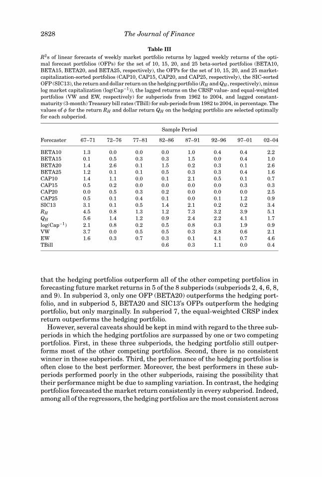
Table IIIR2s of linear forecasts of weekly market portfolio returns by lagged weekly returns of the opti-
mal forecast portfolios (OFPs) for the set of 10, 15, 20, and 25 beta-sorted portfolios (BETA10,
BETA15, BETA20, and BETA25, respectively), the OFPs for the set of 10, 15, 20, and 25 market-
capitalization-sorted portfolios (CAP10, CAP15, CAP20, and CAP25, respectively), the SIC-sorted
OFP (SIC13), the return and dollar return on the hedging portfolio (RH and QH , respectively), minus
log market capitalization (log(Cap−1)), the lagged returns on the CRSP value- and equal-weighted
portfolios (VW and EW, respectively) for subperiods from 1962 to 2004, and lagged constant-
maturity (3-month) Treasury bill rates (TBill) for sub-periods from 1982 to 2004, in percentage. The
values of φ for the return RH and dollar return QH on the hedging portfolio are selected optimally
for each subperiod.
Sample Period
Forecaster 67–71 72–76 77–81 82–86 87–91 92–96 97–01 02–04
BETA10 1.3 0.0 0.0 0.0 1.0 0.4 0.4 2.2
BETA15 0.1 0.5 0.3 0.3 1.5 0.0 0.4 1.0
BETA20 1.4 2.6 0.1 1.5 0.2 0.3 0.1 2.6
BETA25 1.2 0.1 0.1 0.5 0.3 0.3 0.4 1.6
CAP10 1.4 1.1 0.0 0.1 2.1 0.5 0.1 0.7
CAP15 0.5 0.2 0.0 0.0 0.0 0.0 0.3 0.3
CAP20 0.0 0.5 0.3 0.2 0.0 0.0 0.0 2.5
CAP25 0.5 0.1 0.4 0.1 0.0 0.1 1.2 0.9
SIC13 3.1 0.1 0.5 1.4 2.1 0.2 0.2 3.4
RH 4.5 0.8 1.3 1.2 7.3 3.2 3.9 5.1
QH 5.6 1.4 1.2 0.9 2.4 2.2 4.1 1.7
log(Cap−1) 2.1 0.8 0.2 0.5 0.8 0.3 1.9 0.9
VW 3.7 0.0 0.5 0.5 0.3 2.8 0.6 2.1
EW 1.6 0.3 0.7 0.3 0.1 4.1 0.7 4.6
TBill 0.6 0.3 1.1 0.0 0.4
that the hedging portfolios outperform all of the other competing portfolios inforecasting future market returns in 5 of the 8 subperiods (subperiods 2, 4, 6, 8,and 9). In subperiod 3, only one OFP (BETA20) outperforms the hedging port-folio, and in subperiod 5, BETA20 and SIC13’s OFPs outperform the hedgingportfolio, but only marginally. In subperiod 7, the equal-weighted CRSP indexreturn outperforms the hedging portfolio.
However, several caveats should be kept in mind with regard to the three sub-periods in which the hedging portfolios are surpassed by one or two competingportfolios. First, in these three subperiods, the hedging portfolio still outper-forms most of the other competing portfolios. Second, there is no consistentwinner in these subperiods. Third, the performance of the hedging portfolios isoften close to the best performer. Moreover, the best performers in these sub-periods performed poorly in the other subperiods, raising the possibility thattheir performance might be due to sampling variation. In contrast, the hedgingportfolios forecasted the market return consistently in every subperiod. Indeed,among all of the regressors, the hedging portfolios are the most consistent across

Trading Volume 2829
all 8 subperiods, a remarkable confirmation of the properties of the model ofSections I and II.20
V. The Hedging-Portfolio Return as a Risk Factor
To evaluate the success of the hedging portfolio return as a risk factor inthe cross section of expected returns, we implement a slightly modified ver-sion of the well known regression tests outlined in Fama and MacBeth (1973).The basic approach is the same: Form portfolios sorted by an estimated pa-rameter such as market beta coefficients in one time period (the “portfolio-formation period”), estimate betas for those same portfolios in a second nonover-lapping time period (the “estimation period”), and perform a cross-sectional re-gression test for the explanatory power of those betas using the returns ofa third nonoverlapping time period (the “testing period”). However, in con-trast to Fama and MacBeth (1973), we use weekly instead of monthly re-turns, and our portfolio formation, estimation, and testing periods are 5 yearseach.21
Specifically, we run the following bivariate regression for each security inthe portfolio formation period, using only those securities that exist in all threeperiods:22
Rjt = α j + βMj RMt + βH
j RHt + εit, (44)
where RMt is the return on the CRSP value-weighted index and RHt is thereturn on the hedging portfolio. Using the estimated coefficients {βM
i } and {βHi },
we perform a double sort among the individual securities in the estimationperiod, creating 100 portfolios corresponding to the deciles of the estimatedmarket and hedging portfolio betas. We re-estimate the two betas for each ofthese 100 portfolios in the estimation period, and use these estimated betasas regressors in the testing period, for which we estimate the following cross-sectional regression:
Rpt = γ0t + γ1t βMp + γ2t β
Hp + ηpt, (45)
20 On the other hand, the results in Table III must be tempered by the fact that the OFPs are
only as good as the basis portfolios from which they are constructed. Increasing the number of basis
portfolios should, in principle, increase the predictive power of the OFP. However, as the number
of basis portfolios increases, the estimation errors in the autocovariance estimators γ0 and γ1 also
increase for a fixed set of time-series observations, thus the impact on the predictive power of the
OFP is not clear.21 Our first portfolio formation period, from 1962 to 1966, is only 41/2 years because the CRSP
Daily Master file begins in July 1962. Fama and MacBeth’s (1973) original procedure uses a 7-year
portfolio formation period, a 5-year estimation period, and a 4-year testing period.22 This induces a certain degree of survivorship bias since our sample requires that stocks be
listed for at least 15 years. While survivorship bias has a clear impact on expected returns and on
the size effect, its implications for the cross-sectional explanatory power of the hedging portfolio
are less obvious, hence we proceed cautiously with this selection criterion.

2830 The Journal of Finance
where Rpt is the equal-weighted portfolio return for securities in portfolio p,p = 1, . . . , 100, which we construct from the double-sorted rankings of the port-folio estimation period, and βM
pt and βHpt are the market and hedging-portfolio
returns, respectively, of portfolio p that we obtain from the estimation period.This cross-sectional regression is estimated for each of the 261 weeks in the5-year testing period, yielding a time series of coefficients {γ0t}, {γ1t}, and {γ2t}.This entire procedure is repeated by incrementing the portfolio formation, esti-mation, and testing periods by 5 years. We then perform the same analysis forthe hedge portfolio dollar return series {QHt}.
Because we use weekly instead of monthly data, it may be difficult to compareour results to other cross-sectional tests in the extant literature, for example,Fama and French (1992). Therefore, we apply our procedure to four other bench-mark models: The standard CAPM in which RMt is the only regressor in (44);a two-factor model in which the hedging portfolio return factor is replaced bya “small-minus-big capitalization” or “SMB” portfolio return factor as in Famaand French (1992); a two-factor model in which the hedging-portfolio returnfactor is replaced by the OFP return factor described in Subsection B;23 anda three-factor model in which both SMB and high-minus-low book-to-market(HML) factors are included along with the market factor, that is
Rpt = γ0t + γ1t βMp + γ2t β
SMBp + γ3t β
HMLp + ηpt. (46)
Table IV reports correlations in subperiods 1, 8, and 9 among the differentportfolio return factors, returns on CRSP value- and equal-weighted portfolios,the return and dollar return on the hedging portfolio, returns on the SMBportfolio, the return on OFP BETA20, and the two turnover indices (see Lo andWang (2005) for summary statistics for the return betas from the six linearfactor models).
Table V summarizes the results of all of these cross-sectional regression testsfor each of the seven testing periods from 1972 to 2004. In the first subpanel,which corresponds to the first testing period from 1972 to 1976, there is littleevidence in support of the CAPM or any of the other linear models we esti-mate.24 For example, the first three rows show that the time-series averageof the market beta coefficients, {γ1t}, is 0.0%, with a t-statistic of 0.35 and anaverage R2 of 10.0%.25 When the hedging portfolio beta βH
t is added to the
23 Specifically, the SMB portfolio return is constructed by taking the difference of the value-
weighted returns of securities with market capitalization below and above the median market
capitalization at the start of the 5-year subperiod.24 The two-factor model with OFP as the second factor is not estimated until the second testing
period because we use the 1962 to 1966 period to estimate the covariances from which the OFP
returns in the 1967 to 1971 period are constructed. Therefore, the OFP returns are not available
in the first portfolio formation period.25 The t-statistic is computed under the assumption of independently and identically distributed
coefficients {γ 1t}, which may not be appropriate. However, since this has become the standard
method for reporting the results of these cross-sectional regression tests, we follow this convention
to make our results comparable to those in the literature.

Trading Volume 2831
Table IVCorrelation matrix for weekly returns on the CRSP value-weighted index (RVWt), the CRSP equal-
weighted index (REWt), the hedging portfolio return (RHt), the hedging portfolio dollar return (QHt),
the return of the small-minus-big capitalization stocks portfolio (RSMBt), the return of the high-
minus-low book-to-market stocks portfolio (RHMLt), the return ROFPt of the optimal forecast portfolio
(OFP) for the set of 20 market-beta-sorted basis portfolios, and the equal-weighted and share-
weighted turnover indices (τEWt and τSW
t ), using CRSP weekly returns and volume data for NYSE
and AMEX stocks for three subperiods: January 1967 – December 1971, January 1997 – December
2001, and January 2002 – December 2004.
RVWt REWt RHt QHt RSMBt RHMLt ROFPt τEWt τSW
t
January 1967 – December 1971 (261 Weeks)
RVWt 100.0 92.6 95.6 91.5 62.7 −44.1 −76.2 19.1 26.3
REWt 92.6 100.0 92.3 88.4 84.5 −40.8 −71.9 32.8 36.9
RHt 95.6 92.3 100.0 97.4 70.7 −52.4 −65.0 22.0 29.6
QHt 91.5 88.4 97.4 100.0 69.8 −49.4 −60.1 22.9 29.8
RSMBt 62.7 84.5 70.7 69.8 100.0 −40.6 −46.6 39.7 38.2
RHMLt −44.1 −40.8 −52.4 −49.4 −40.6 100.0 14.5 −9.0 −15.0
ROFPt −76.2 −71.9 −65.0 −60.1 −46.6 14.5 100.0 −7.5 −10.4
τEWt 19.1 32.8 22.0 22.9 39.7 −9.0 −7.5 100.0 93.1
τSWt 26.3 36.9 29.6 29.8 38.2 −15.0 −10.4 93.1 100.0
January 1997 – December 2001 (261 Weeks)
RVWt 100.0 80.4 57.9 43.4 −20.7 −48.7 −45.7 3.3 −0.9
REWt 80.4 100.0 54.8 42.6 24.9 −46.7 −33.1 7.9 −1.4
RHt 57.9 54.8 100.0 89.2 17.0 −71.0 −15.5 0.0 −2.2
QHt 43.4 42.6 89.2 100.0 25.3 −70.0 −1.2 3.8 0.4
RSMBt −20.7 24.9 17.0 25.3 100.0 −41.8 25.8 7.0 0.1
RHMLt −48.7 −46.7 −71.0 −70.0 −41.8 100.0 2.5 −0.1 4.4
ROFPt −45.7 −33.1 −15.5 −1.2 25.8 2.5 100.0 −0.9 1.8
τEWt 3.3 7.9 0.0 3.8 7.0 −0.1 −0.9 100.0 92.4
τSWt −0.9 −1.4 −2.2 0.4 0.1 4.4 1.8 92.4 100.0
January 2002 – December 2004 (156 Weeks)
RVWt 100.0 91.8 68.6 −11.5 −17.1 −6.6 55.0 9.3 4.1
REWt 91.8 100.0 76.3 −32.7 15.8 10.2 50.3 5.5 −3.1
RHt 68.6 76.3 100.0 −60.4 14.1 −2.0 31.5 5.4 −0.4
QHt −11.5 −32.7 −60.4 100.0 −56.5 −2.4 −2.5 −3.9 3.3
RSMBt −17.1 15.8 14.1 −56.5 100.0 9.4 −7.2 −5.6 −9.1
RHMLt −6.6 10.2 −2.0 −2.4 9.4 100.0 −17.2 −18.3 −27.9
ROFPt 55.0 50.3 31.5 −2.5 −7.2 −17.2 100.0 12.1 3.7
τEWt 9.3 5.5 5.4 −3.9 −5.6 −18.3 12.1 100.0 77.8
τSWt 4.1 −3.1 −0.4 3.3 −9.1 −27.9 3.7 77.8 100.0
regression, the R2 increases to 14.3% but the average of the coefficients {γ2t}is −0.2% with a t-statistic of −0.82. The average market beta coefficient is stillinsignificant, but it has now switched sign. The results for the two-factor modelwith the hedging portfolio dollar return factor and the two-factor model withthe SMB factor are similar. The three-factor model is even less successful, withstatistically insignificant coefficients close to 0.0% and an average R2 of 8.8%.
In the second testing period, both specifications with the hedging portfoliofactor exhibit statistically significant means for the hedging portfolio betas,

2832 The Journal of Finance
Table VCross-sectional regression tests of six linear factor models along the lines of Fama and MacBeth
(1973), using weekly returns for NYSE and AMEX stocks from 1962 to 2004 in 5-year subperiods
for the portfolio formation, estimation, and testing periods, and 100 portfolios in the cross-sectional
regressions each week. The six linear factor models are: the standard CAPM (βMp ); four two-factor
models in which the first factor is the market beta and the second factors are, respectively, the
hedging portfolio return beta (βHRp ), the hedging portfolio dollar return beta (β
HQp ), the beta of a
small-minus-big cap portfolio return (βSMBp ), the beta of the Fama and French (1992) high-minus-
low book-to-market portfolio return (βHMLp ), and the beta of the optimal forecast portfolio based on
a set of 25 market-beta-sorted basis portfolios (βOFPp ); and a three-factor model with βM
p , βSMBp , and
βHMLp as the three factors.
Model Statistic γ0t γ1t γ2t γ3t R2(%)
January 1972 – December 1976 (261 Weeks)
Rpt = γ0t + γ1t βMp + εpt Mean (%): 0.2 0.0 10.0
S.D. (%): 1.5 2.1 10.9
t-stat: 1.64 0.35
Rpt = γ0t + γ1t βMp + γ2t β
H Rp + εpt Mean (%): 0.4 −0.2 −0.2 14.3
(φ = 1.25) S.D. (%): 3.5 3.5 3.7 10.9
t-stat: 2.04 −1.05 −0.82
Rpt = γ0t + γ1t βMp + γ2t β
H Qp + εpt Mean (%): 0.4 −0.2 −10.4 15.5
(φ = 1.50) S.D. (%): 3.2 3.4 379.7 10.9
t-stat: 2.16 −1.08 −0.44
Rpt = γ0t + γ1t βMp + γ2t β
SM Bp + εpt Mean (%): 0.1 0.0 6.3 12.1
S.D. (%): 1.4 2.4 114.2 10.8
t-stat: 1.42 0.22 0.90
Rpt = γ0t + γ1t βMp + γ2t β
H M Lp + εpt Mean (%): 0.0 0.1 0.2 7.8
S.D. (%): 1.8 1.9 1.5 7.8
t-stat: 0.40 1.08 1.66
Rpt = γ0t + γ1t βMp + γ2t β
SM Bp + γ3t β
H M Lp + εpt Mean (%): 0.0 0.1 0.0 0.1 8.8
S.D. (%): 1.8 2.1 1.2 1.5 7.6
t-stat: 0.28 0.80 0.50 1.27
January 1977 – December 1981 (261 Weeks)
Rpt = γ0t + γ1t βMp + εpt Mean (%): 0.1 0.3 11.7
S.D. (%): 1.1 2.2 12.8
t-stat: 1.17 2.57
Rpt = γ0t + γ1t βMp + γ2t β
H Rp + εpt Mean (%): 0.3 −0.1 −1.2 13.1
(φ = 4.75) S.D. (%): 1.4 2.0 5.1 12.4
t-stat: 3.75 −0.90 −3.71
Rpt = γ0t + γ1t βMp + γ2t β
H Qp + εpt Mean (%): 0.3 −0.1 −156.4 12.5
(φ = 4.25) S.D. (%): 1.3 2.0 610.4 12.2
t-stat: 3.91 −0.75 −4.14
Rpt = γ0t + γ1t βMp + γ2t β
SM Bp + εpt Mean (%): 0.1 0.0 29.9 14.9
S.D. (%): 1.1 1.7 108.8 13.4
t-stat: 2.25 −0.16 4.43
Rpt = γ0t + γ1t βMp + γ2t β
H M Lp + εpt Mean (%): 0.2 0.2 0.1 9.3
S.D. (%): 1.3 1.9 0.9 9.2
t-stat: 2.15 1.52 1.58
Rpt = γ0t + γ1t βMp + γ2t β
O F Pp + εpt Mean (%): 0.3 0.1 0.1 14.1
S.D. (%): 1.8 2.3 3.6 11.6
t-stat: 2.74 0.84 0.63
Rpt = γ0t + γ1t βMp + γ2t β
SM Bp + γ3t β
H M Lp + εpt Mean (%): 0.2 −0.0 0.3 −0.1 11.5
S.D. (%): 1.2 1.7 1.0 1.0 10.0
t-stat: 2.72 −0.07 4.61 −0.85
(continued)

Trading Volume 2833
Table V—Continued
January 1982 – December 1986 (261 Weeks)
Rpt = γ0t + γ1t βMp + εpt Mean (%): 0.6 −0.1 9.4
S.D. (%): 1.1 1.9 11.1
t-stat: 8.17 −1.04
Rpt = γ0t + γ1t βMp + γ2t β
H Rp + εpt Mean (%): 0.6 −0.1 −0.6 9.6
(φ = 1.75) S.D. (%): 1.1 2.0 5.5 9.4
t-stat: 8.39 −0.78 −1.73
Rpt = γ0t + γ1t βMp + γ2t β
H Qp + εpt Mean (%): 0.6 −0.2 −74.0 10.4
(φ = 2.00) S.D. (%): 1.1 1.9 1987.4 9.5
t-stat: 8.36 −1.30 −0.60
Rpt = γ0t + γ1t βMp + γ2t β
SM Bp + εpt Mean (%): 0.5 −0.2 3.8 10.0
S.D. (%): 1.2 1.9 115.4 8.4
t-stat: 7.45 −1.26 0.53
Rpt = γ0t + γ1t βMp + γ2t β
H M Lp + εpt Mean (%): 0.5 −0.1 0.2 9.2
S.D. (%): 1.4 1.9 1.5 8.5
t-stat: 5.57 −0.83 1.81
Rpt = γ0t + γ1t βMp + γ2t β
O F Pp + εpt Mean (%): 0.5 −0.1 0.0 11.7
S.D. (%): 1.1 2.0 2.1 10.8
t-stat: 7.55 −0.82 0.20
Rpt = γ0t + γ1t βMp + γ2t β
SM Bp + γ3t β
H M Lp + εpt Mean (%): 0.4 −0.0 0.0 0.1 10.0
S.D. (%): 1.4 2.2 1.0 1.1 8.5
t-stat: 4.49 −0.24 0.55 1.97
January 1987 – December 1991 (261 Weeks)
Rpt = γ0t + γ1t βMp + εpt Mean (%): 0.2 5.9
S.D. (%): 1.3 2.3 8.7
t-stat: 2.65 0.20
Rpt = γ0t + γ1t βMp + γ2t β
H Rp + εpt Mean (%): 0.2 0.0 0.0 5.4
(φ = 47) S.D. (%): 1.6 1.9 6.0 6.1
t-stat: 2.25 0.11 0.13
Rpt = γ0t + γ1t βMp + γ2t β
H Qp + εpt Mean (%): 0.2 0.0 18.9 6.0
(φ = 20) S.D. (%): 1.6 1.9 1819.4 6.7
t-stat: 2.43 −0.15 0.17
Rpt = γ0t + γ1t βMp + γ2t β
SM Bp + εpt Mean (%): 0.3 0.0 −7.5 7.8
S.D. (%): 1.4 2.0 123.5 8.2
t-stat: 3.10 0.16 −0.98
Rpt = γ0t + γ1t βMp + γ2t β
H M Lp + εpt Mean (%): 0.2 0.0 0.0 6.3
S.D. (%): 1.6 2.0 1.8 7.6
t-stat: 2.11 0.03 −0.38
Rpt = γ0t + γ1t βMp + γ2t β
O F Pp + εpt Mean (%): 0.3 −0.1 0.0 6.4
S.D. (%): 1.5 2.1 2.1 7.3
t-stat: 2.73 −0.39 −0.23
Rpt = γ0t + γ1t βMp + γ2t β
SM Bp + γ3t β
H M Lp + εpt Mean (%): 0.3 0.0 −0.1 −0.1 7.8
S.D. (%): 1.9 2.1 1.2 1.5 6.8
t-stat: 2.21 0.16 −0.97 −1.10
(continued)
with average coefficients and t-statistics of −1.2% and −3.71 for the hedging-portfolio return factor and −1.56 and −4.14 for the hedging portfolio dollarreturn factor, respectively. In contrast, the market beta coefficients are notsignificant in either of these specifications, and are also of the wrong sign. Theonly other specifications with a significant mean coefficient are the two-factormodel with SMB as the second factor (with an average coefficient of 29.9% for
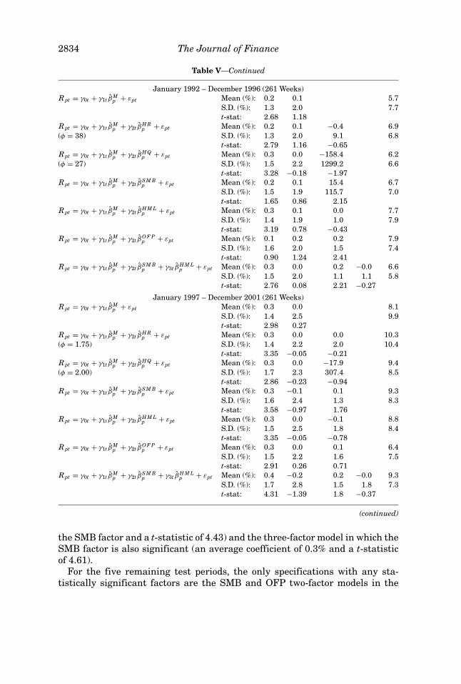
2834 The Journal of Finance
Table V—Continued
January 1992 – December 1996 (261 Weeks)
Rpt = γ0t + γ1t βMp + εpt Mean (%): 0.2 0.1 5.7
S.D. (%): 1.3 2.0 7.7
t-stat: 2.68 1.18
Rpt = γ0t + γ1t βMp + γ2t β
H Rp + εpt Mean (%): 0.2 0.1 −0.4 6.9
(φ = 38) S.D. (%): 1.3 2.0 9.1 6.8
t-stat: 2.79 1.16 −0.65
Rpt = γ0t + γ1t βMp + γ2t β
H Qp + εpt Mean (%): 0.3 0.0 −158.4 6.2
(φ = 27) S.D. (%): 1.5 2.2 1299.2 6.6
t-stat: 3.28 −0.18 −1.97
Rpt = γ0t + γ1t βMp + γ2t β
SM Bp + εpt Mean (%): 0.2 0.1 15.4 6.7
S.D. (%): 1.5 1.9 115.7 7.0
t-stat: 1.65 0.86 2.15
Rpt = γ0t + γ1t βMp + γ2t β
H M Lp + εpt Mean (%): 0.3 0.1 0.0 7.7
S.D. (%): 1.4 1.9 1.0 7.9
t-stat: 3.19 0.78 −0.43
Rpt = γ0t + γ1t βMp + γ2t β
O F Pp + εpt Mean (%): 0.1 0.2 0.2 7.9
S.D. (%): 1.6 2.0 1.5 7.4
t-stat: 0.90 1.24 2.41
Rpt = γ0t + γ1t βMp + γ2t β
SM Bp + γ3t β
H M Lp + εpt Mean (%): 0.3 0.0 0.2 −0.0 6.6
S.D. (%): 1.5 2.0 1.1 1.1 5.8
t-stat: 2.76 0.08 2.21 −0.27
January 1997 – December 2001 (261 Weeks)
Rpt = γ0t + γ1t βMp + εpt Mean (%): 0.3 0.0 8.1
S.D. (%): 1.4 2.5 9.9
t-stat: 2.98 0.27
Rpt = γ0t + γ1t βMp + γ2t β
H Rp + εpt Mean (%): 0.3 0.0 0.0 10.3
(φ = 1.75) S.D. (%): 1.4 2.2 2.0 10.4
t-stat: 3.35 −0.05 −0.21
Rpt = γ0t + γ1t βMp + γ2t β
H Qp + εpt Mean (%): 0.3 0.0 −17.9 9.4
(φ = 2.00) S.D. (%): 1.7 2.3 307.4 8.5
t-stat: 2.86 −0.23 −0.94
Rpt = γ0t + γ1t βMp + γ2t β
SM Bp + εpt Mean (%): 0.3 −0.1 0.1 9.3
S.D. (%): 1.6 2.4 1.3 8.3
t-stat: 3.58 −0.97 1.76
Rpt = γ0t + γ1t βMp + γ2t β
H M Lp + εpt Mean (%): 0.3 0.0 −0.1 8.8
S.D. (%): 1.5 2.5 1.8 8.4
t-stat: 3.35 −0.05 −0.78
Rpt = γ0t + γ1t βMp + γ2t β
O F Pp + εpt Mean (%): 0.3 0.0 0.1 6.4
S.D. (%): 1.5 2.2 1.6 7.5
t-stat: 2.91 0.26 0.71
Rpt = γ0t + γ1t βMp + γ2t β
SM Bp + γ3t β
H M Lp + εpt Mean (%): 0.4 −0.2 0.2 −0.0 9.3
S.D. (%): 1.7 2.8 1.5 1.8 7.3
t-stat: 4.31 −1.39 1.8 −0.37
(continued)
the SMB factor and a t-statistic of 4.43) and the three-factor model in which theSMB factor is also significant (an average coefficient of 0.3% and a t-statisticof 4.61).
For the five remaining test periods, the only specifications with any sta-tistically significant factors are the SMB and OFP two-factor models in the

Trading Volume 2835
Table V—Continued
January 2002 – December 2004 (156 Weeks)
Rpt = γ0t + γ1t βMp + εpt Mean (%): 0.4 0.0 3.9
S.D. (%): 1.7 1.3 4.2
t-stat: 3.26 −0.27
Rpt = γ0t + γ1t βMp + γ2t β
H Rp + εpt Mean (%): 0.6 −0.2 0.6 9.3
(φ = 1.75) S.D. (%): 1.7 2.5 8.0 9.6
t-stat: 4.54 −0.94 0.94
Rpt = γ0t + γ1t βMp + γ2t β
H Qp + εpt Mean (%): 0.7 −0.3 −106.5 5.8
(φ = 2.00) S.D. (%): 2.2 2.2 699.7 6.2
t-stat: 4.29 −1.71 −1.90
Rpt = γ0t + γ1t βMp + γ2t β
SM Bp + εpt Mean (%): 0.5 −0.1 0.1 4.2
S.D. (%): 2.2 0.7 0.6 4.9
t-stat: 2.71 −1.43 1.59
Rpt = γ0t + γ1t βMp + γ2t β
H M Lp + εpt Mean (%): 0.5 −0.1 0.0 6.1
S.D. (%): 2.0 1.4 1.0 5.4
t-stat: 3.17 −0.86 −0.55
Rpt = γ0t + γ1t βMp + γ2t β
O F Pp + εpt Mean (%): 0.4 0.0 0.0 4.1
S.D. (%): 1.7 1.3 0.4 4.0
t-stat: 3.15 0.01 −0.19
Rpt = γ0t + γ1t βMp + γ2t β
SM Bp + γ3t β
H M Lp + εpt Mean (%): 0.4 0.0 0.0 0.1 5.8
S.D. (%): 2.4 0.5 0.4 1.1 5.3
t-stat: 2.03 0.03 1.57 0.75
1992–1996 testing period though the hedging portfolio dollar return factor isclose to significant in the 1997–2001 subperiod. However, the R2s in the lastfour testing periods are substantially lower than in the earlier periods, perhapsreflecting the greater volatility of equity returns in recent years.
Overall, the results do not provide overwhelming support for any factor inexplaining the cross-sectional variation of expected returns. There is, of course,the ubiquitous problem of lack of power in these cross-sectional regression tests,hence we should not be surprised that no single factor stands out (see e.g.,MacKinlay (1987, 1994)). However, the point estimates of the cross-sectionalregressions show that the hedging portfolio factor is comparable both in mag-nitude and in performance to other commonly proposed factors, and yields apromising new direction for intertemporal asset pricing research.
VI. Conclusion
By deriving an explicit link between economic fundamentals and the dynamicproperties of asset returns and volume, we have shown that interactions be-tween prices and quantities in equilibrium yield a rich set of implications forany asset-pricing model. Indeed, by exploiting the relation between prices andvolume in our dynamic equilibrium model, we are able to identify and constructthe hedging portfolio that all investors use to hedge against changes in marketconditions. Moreover, our empirical analysis shows that this hedging portfo-lio has considerable forecast power in predicting future returns of the market

2836 The Journal of Finance
portfolio—a property of the true hedging portfolio—and its abilities to explaincross-sectional variation in expected returns is comparable to other popularrisk factors such as market betas, the Fama and French (1992) SMB and HMLfactors, and optimal forecast portfolios.
Although, our model is purposefully parsimonious so as to focus attention onthe essential features of risk-sharing and trading activity, it underscores thegeneral point that quantities, together with prices, should be an integral part ofany analysis of asset markets, both theoretically and empirically, as our resultsclearly indicate.
Appendix: Proofs
Proof of Theorem 1: We prove Theorem 1 by first deriving investor assetdemand under the price function (9) and then solving the coefficient vectors aand b to clear the stock market.
For simplicity in notation, let ut ≡ (Dt; Xt), where (· ; ·) denotes a column vectorand (· , ·) denotes a row vector. From (9), we have
Qt+1 = Q t + Q t+1, (A1)
where Q t = ra + (1+r)bX t , Q t+1 = (1, −b)ut+1, and 1 is an (j × j) identitymatrix.
We now consider investor i’s optimal portfolio choice. Let St be the vector ofhis stock holding in period t. His next period wealth is Wt+1 = Wt + St
′ Q t+1 +St
′(1, −b)ut+1, where we have omitted superscript i for brevity. We also let λ1t ≡λXXt + λYYt and λ2t ≡ λZ(1 + Zt). Then,
Et
[e−Wt+1−λ1t DMt+1−λ2t X t+1
] = Et
[e−Wt−St
′ Q t+(St+λ1t ι;−b′St+λ2t )′ut+1
](A2)
= e−Wt−St
′ Q t+1
2
(St + λ1t ι; −b′St + λ2t
)′σ(St + λ1t ι; −b′St + λ2t
), (A3)
where σ is the covariance matrix of ut. The investor’s optimization problemthen reduces to
maxSt
S′t Q t − 1
2
(St + λ1t ι; −b′St + λ2t
)′σ(St + λ1t ι; −b′St + λ2t
). (A4)
The first-order condition is
0 = Q t − (σDD − bσDX
′ − σDXb′ + σXXbb′)St
−λ1t(σDD − bσXD)ι − λ2t(σDX − bσXX ).(A5)
The solution gives the investor’s stock demand
St = (σDD − bσDX
′ − σDXb′ + σXXbb′)−1[Q t − λ1t(σDD − bσDZ)ι − λ2t(σXD − bσXX )].
(A6)

Trading Volume 2837
Summing (A5) over all investors and imposing the market-clearing condition,∑i Si
t = SM , we have
0 = [ra + (1 + r)bXt] − (1/I )σQQSM − λX σQDιX t − λZ σQX . (A7)
It follows that
ra = (1/I )σQQ SM + λZ σQX (A8)
(1 + r)b = λX σQD SM , (A9)
which uniquely determine the equilibrium a and b. Substituting (A7) into (A6),we obtain investor i’s equilibrium stock holding
Sit = (
I−1 − λY Y it
)SM − [
λY (b′SM )Y it + λZ Z i
t
](σQ Q )−1σQ X , (A10)
which is (10). Q.E.D.
Proof of Proposition 1: Let x = �hMt, y = θH�hHt (we omit superscripts i andj for notational simplicity), x′ = x/σx, y′ = y/σy, and η = σy/σx. We can write|x + y| = σx|x′ + ηy′|. Without loss of generality, we let σ x = 1. Since Yt andZt are normal, x′ and y′ are also jointly normal with unit standard deviations.We can write
|x + y | = |x ′ + η y ′| = |x ′| + η Sign(x ′) y ′ + 1D(x ′,η y ′)δ(x ′, η y ′), (A11)
where the last term is defined by the functions D(z1, z2) = {z1z2 < 0, >
|z1| < |z2|} and δ(z1, z2) = −2|z1| + 2|z2|. To assess the statistical error of theapproximation
|x ′ + η y | ≈ |x| + η Sign(x) y , (A12)
we compute the expected approximation error using any loss function L(|.|)that is nonnegative, nondecreasing on R+, and of order α > 0, that is,limε→0L(|ε|)/εα = A exists and is finite. Loss functions satisfying these con-ditions include the mean absolute error (L(z) = |z|, α = 1) and mean squarederror (L(z) = z2, α = 2) loss functions. We then have
E[L(|1D(x,η y)δ(x, η y)|)] = P (D)E[L(|δ(x, η y)|)|D], (A13)
where P (D) = ∫ ∞0
∫ η y ′
0[ f (−x ′, y ′) + f (x ′, − y ′)] dx′ dy′. Let ρ denote the correla-
tion between x′ and y ′. On D, we have f (−x ′, y ′) ≤ 12π
e−(1−ρ2) y ′2/2. It immediatelyfollows that P(D)/η ≤ c, where c is a positive constant. We then have
E[L(|1D(x ′,η y ′)δ(x ′, η y ′)|)] < Aηα+1 + o(ηα+1), (A14)
where A is a constant. Thus, even though the point-wise properties of the ap-proximation are not satisfactory, the approximation error is small in a statisti-cal sense for small η, that is, the expected loss decreases faster than ηα+1. The

2838 The Journal of Finance
definition of η shows that it depends the ratio of volatility of �hHt to �hMt. Asufficient condition is λX , λZ/λY � 1. Q.E.D.
Proof of Proposition 2: Suppose we use the (dollar) return of portfolio S topredict future market returns. The resulting R2 is
R2 = (Cov[(S′Qt)Q Mt+1]
)2/(Var[S′Qt]Var[Q Mt+1]
). (A15)
To choose the S to maximize R2, we solve the following problem
maxS
S′σQX (b′SM ) (A16)
s.t. S′σQQS = v. (A17)
Up to a scaling constant, the solution is SH = (σQQ)−1σQX . Q.E.D.
Proof of Proposition 3: When X t = 0, ∀ t, Qt = ra + Q t = (SM , −b)ut . Then,Cov[Q t , Q Mt] = Cov[Q t , S′
M Qt] = σDD SM , Var[Q Mt] = S′M σDD SM , and (22)
follows. Since σQX = 0 in this case, σMH = 0 and Q M = (1/I )σ 2M . Thus,
Q = βM Q M which is (24). Q.E.D.
Proof of Proposition 4: Equation (25) simply follows from the joint normalityof Q t+1, Q Mt+1, and Q Ht+1. Equation (28) can be verified by substituting in theexpressions for βM , βM , Q M , and Q H , which gives (21c). Q.E.D.
Proof of Proposition 5: Let Qt denote the (dollar) return vector of a set of as-sets, 0 ≡ Cov[QtQt
′] and 1 ≡ Cov[Qt+1Qt′]. Suppose that Sa is a target port-
folio and Sb is a forecasting portfolio whose return is used as a forecast for thereturn on Sa next period. Then, the R2 from the forecast is
R2 = (Cov[S′bQt , S′
a Qt+1])2
Var[S′bQt]Var[S′
a Qt+1]= (S′
b 1Sa)2
(S′a 0Sa)(S′
b 1Sb). (A18)
The OFP for a given Sa is the portfolio that gives the highest R2. In other words,
SOFP = arg max R2 = arg max(S′
b 1Sa)2
(S′a 0Sa)(S′
b 0Sb). (A19)
The optimality condition becomes( −1
0 1SaS′a ′
1
)SOFP = R2(S′
a 0Sa) SOFP. (A20)
It then immediately follows that SOFP is the eigenvector corresponding to thelargest eigenvalue of matrix −1
0 1SaSa′ ′
1, which should equal R2(Sa′ 0Sa).
Although, we derive the result in Proposition 5 using dollar returns andasset shares in defining portfolios, the same result holds if we use rates ofreturn and dollar weights in defining portfolios, which is what the propositionstates. Q.E.D.

Trading Volume 2839
The set of assets considered above does not have to be the entire universe ofassets. In the event it is and expected asset returns are driven by a single statevariable, as in (12), we have
1 = (1 + r) σX bb′ = σQXσ ′QX . (A21)
It then follows that SOFP = SH up to a scaling coefficient, as Proposition 2shows.
REFERENCESAbel, Andrew B., 1990, Asset prices under habit formation and catching up with the Joneses,
American Economic Review 80, 38–42.
Andersen, Torben G., 1996, Return volatility and trading volume: An information flow interpreta-
tion, Journal of Finance 51, 169–204.
Archarya, Viral V., and Lasse H. Pedersen, 2002, Asset pricing with liquidity risk, Journal ofFinancial Economics 2005, 375–410.
Brennan, Michael, and Avanidhar Subrahmanyam, 1996, Market microstructure and asset pricing:
On the compensation for illiquidity in stock returns, Journal of Financial Economics 41, 441–
464.
Campbell, John, and John Cochrane, 1999, By force of habit: A consumption-based explanation of
aggregate stock market behavior, Journal of Political Economy 107, 205–251.
Campbell, J., Grossman, S., and J. Wang, 1993. Trading volume and serial correlation in stock
returns. Quarterly Journal of Economics 108, 905–939.
Chordia, Tarun, Richard Roll, and Avanidhar Subrahmanyam, 2000, Commonality in liquidity,
Journal of Financial Economics 56, 3–28.
Fama, Eugene F., and Kenneth French, 1992, The cross section of expected stock returns, Journalof Finance 47, 427–465.
Fama, Eugene F., and James D. MacBeth, 1973, Risk, return, and equilibrium: Empirical tests,
Journal of Political Economy 81, 607–636.
Foster, Douglas, Tom Smith, and Richard Whaley, 1997, Assessing goodness-of-fit of asset
pricing models: The distribution of the maximal R-squared, Journal of Finance 52, 591–
607.
Gallant, Ronald, Peter E. Rossi, and George Tauchen, 1992, Stock prices and volume, Review ofFinancial Studies 5, 199–242.
Lim, Terence, Andrew W. Lo, Jiang Wang, and Petr Adamek, 1998, Trading volume and the Mini-
CRSP database: An introduction and user’s guide, MIT Laboratory for Financial Engineering
Working Paper No. LFE–1038–98.
Lo, Andrew W., and Craig MacKinlay, 1997, Maximizing predictability in the stock and bond mar-
kets, Macroeconomic Dynamics 1, 102–134.
Lo, Andrew W., and Jiang Wang, 2000, Trading Volume: Definitions, Data Analysis, and Implica-
tions of Portfolio Theory, Review of Financial Studies 13, 257–300.
Lo, Andrew W., and Jiang Wang, 2003, Trading Volume, in M. Dewatripont, L. Hansen, and S.
Turnovsky, eds.: Advances in Economics and Econometrics: Theory and Applications, EighthWorld Congress, Volume II (Cambridge University Press).
Lo Andrew W., and Jiang Wang, 2005, Trading volume: Implications from an intertemporal asset
pricing model, working paper, MIT.
MacKinlay, Craig, 1987, On multivariate tests of the CAPM, Journal of Financial Economics 18,
341–371.
MacKinlay, Craig, 1994, Multi-factor models do not explain deviations from the CAPM, Journal ofFinancial Economics 38, 3–28.
Merton, Robert C., 1971, Optimal consumption and portfolio rules in a continuous-time model,
Journal of Economic Theory 3, 373–413.

2840 The Journal of Finance
Merton, Robert C., 1973, An intertemporal capital asset pricing model, Econometrica 41, 867–887.
Pastor, Lubos, and Robert F. Stambaugh, 2002, Liquidity risk and expected stock returns, Journalof Political Economy 111, 642–85.
Tkac, Paula, 1996, A trading volume benchmark: Theory and evidence, working paper, Department
of Finance and Business Economics, University of Notre Dame.
Wang, Jiang, 1994, A model of competitive stock trading volume, Journal of Political Economy 102,
127–168.