TRADING THROUGH ARTIFICIAL EYES - linclund.com

TRADING THROUGH

ARTIFICIAL EYESTime Series Classifications Using

Deep Neural Networks

2019-06-15

TRADING & QUANTITATVE RESEARCH REPORT

ANALYSTS: JIM ÖHMAN & JAN MUELLER

Avoid

Level one quotesEUR/USD

Live Price Feed

THESIS, TRADING STRATEGY AND METHOD

Investment Thesis

While making a trade is not uncommon to rely on visual queues, simply

the look of previous price history contains lots of information, such as

current trends and volatility. If it was possible to construct an algorithm

that could see the financial data in a similar way to us humans, maybe it is

also possible to automate trading through its artificial eyes. These types of

algorithms are indeed possible to construct, as advancements in deep

learning has made computer vision powerful and yet relatively easy to

implement. A type of neural network called a Convolutional Neural

Network (CNN) is a state of the art image processing algorithm that

borrow similarities to the workings of human vision. These networks can

be taught to identify objects within an image by giving them labeled

images and training them through a process called back-propagation. They

function by scanning the image with filters that they have learned to find

edges and particular shapes that belong to the objects it is asked to

identify. The output of such a neural net is a probability distribution over

all the classes of objects that it has been trained on.

By assembling windows of historical price data and labelling them given

their overall bullish, bearish and noisy nature, one can train these neural

networks to pick up on characteristic visual queues that can distinguish

these three classes of windows.

A schematic overview of the neural net preparation phase can be seen in

Exhibit A.

Trading Strategy

With these visual queues as inputs, the next question would be what trading

strategy could exploit them. It is possible to add another network that takes

the outputs of the CNN and is trained by reinforcement learning to make it

find its own strategy. But instead of going down that long road, one could

play around with the simple strategy of going long or going short after the

network makes label predictions, based on some pre-determined criteria. It

was found that treating the neural net classifications as indicating local high

or low price levels could be made significantly profitable. The strategy is to

open positions if a given number of bearish or bullish windows have

previously been predicted and satisfies a set of criteria, that is to be

introduced later. This works by placing many positions at the peaks and

troughs of price movements, maximizing the likelihood of profits. This

approach accompanied with a collective take profit and stop loss, as well as a

dynamic take profit level made a successful strategy.

Method

Historical level one quotes are collected from the most liquid currency

pair, the EUR/USD, which span most working days between August

2018 to March 2019, and consists of best bid and best ask values with

millisecond granularity. This data is then sampled into 20 minute

windows, and labelled depending their bullish, bearish or noisy nature,

through a calculation of the average profit or loss by buying and selling

in these windows. The dataset is then split 70% into a training dataset,

and 30% as a test dataset to evaluate the classification performance.

All trading is simulated trough code written in Python, where trading

conditions are made realistic by accounting for spreads, execution fees,

roll over fees and slippage. Additionally, trading on margin is added,

where one can leverage an investment up to 30 times. The system keeps

track of usable margin and will produce a margin call if necessary. The

training dataset is also used to optimize the trading strategy while its

trading performance is evaluated on the test dataset.

As is displayed in Exhibit B, during the trading process, a continuous

feed of price data is to be assembled into windows every minute. New

trades are then made on the fly as the network predicts new labels and

checks the criteria. Trades are then closed once they reach the take

profit or stop loss levels.

LINC – Lund University Finance Society | See disclaimer at the end of the report 1

Exhibit B: Schematic overview of a trading phase. Price data is collected

through a live feed and assembled into window samples for the network to

predict the nature of. Trades are then placed based on the history of predictions.

Level one quotesEUR/USD

Collect Historical Price Data

Determine LabelsCreate Windows

Assemble Dataset

70% of the dataset

Train Neural Net

30% of the dataset

Evaluate Performance

Exhibit A: Schematic overview of the preparation phase. The historical price

data is assembled into a dataset, that is then used to train and evaluate the

networks classification performance.

Input to Neural NetOn the fly

Assemble New Window

Window label prediction

Neural Net Classification

LongShort

Trading Decision

WINDOWS, PERFORMANCE AND VISUALIZATION


Typical Windows

A typical window of each label is presented in Exhibit C. The top window

shows a clear noisy nature, as it contains little information of where the

price might be moving next. The middle window shows a clear bullish

nature, and the bottom window a clear bearish nature. These bottom two

should certainly be more connected to future price movement than the top

one.

All windows have been zeroed around their starting value, then averaged

over intervals of 10 seconds, and normalized to units of pip, which are

increements on the fourth decimal of the price. This is done to aid the

network during training and to reduce computation time. The zeroing

removes any dependance on the actual price, which mean that windows at

the end of the dataset are treated the same as those in the beginning.

Averaging the windows over intervals of 10 seconds reduces the size of the

input, which in turn reduces computation time significantly. The

normalization to units of pip was mainly done for convenience.

Classification Performance

The assembled dataset contains 96826 windows of which 11443 are

labelled as bullish, 12189 are labelled as bearish, and the rest noisy. As can

be seen, there are many more noisy windows than bullish and bearish ones,

which is to be expected if it would capture useful information. The slight

imbalance between the amount of bearish and bullish windows does

indicate an overall drop in average price over the whole dataset, which can

be confirmed.

Training the network for just one hour achieves above 90% accuracy on

both the training and test part of the dataset. This means that very little

overfitting was done and that it managed to find general visual queues that

is able to distinguish these classes well. An interesting note is that no

misclassifications between bullish and bearish labels was made.

Additionally, those windows that were misclassified acutally looks

mislabelled instead, demonstrating the neural nets ability to improve upon

the coarse labelling function.

Network Visualization

A common problem with neural networks is that they hide their decision

making, and in most cases there is no way of knowing why they make the

choices they make. It could be beneficial to see what they have learned in

order to more easily make improvements on them. For Convolutional

Neural Networks (CNN’s) some visualization methods have been

developed, and one of these methods is called a Class Activation Map

(CAM) which requires the network to have a specific architecture, which is

precisely the architecture used in this project. This method takes a window

along with the neural net and colors the price history in different

intensities, with high intensities corresponding to the places the network is

mainly focusing its eyes.

A CAM of the previously displayed noisy, bullish and bearish windows can

be seen in Exhibit D. The network classifies the noisy window corretly as

containing mainly noise, with a little bit of bullish and bearish nature.

According to the intensities, it does look at most of this window during

classification, which could be some sort of internal moving average

calculation. It also classifies the bullish window correctly, but here it is

interesting to note that it focuses mainly on the middle of the upswings

while ignoring the middle of downswings, which is quite a reasonable way

to identify bullish movements. The bearish window is also classified

correctly, and interestingly it is determined to have a bit more noisy nature

than the bullish one, which does seem reasonable when comparing the

appearence of the two. It can also be seen that it focuses on the opposite

for bearish windows than what it does for bullish windows, and that is the

middle of downswings, which again seems reasonable. Both the bullish and

bearish window has focus at the endpoints, which is likely there as the

endpoint value is a way step to differentiate between many bullish and

bearish windows.

20 Minutes

Exhibit C: Three examples of typical noisy, bullish and bearish windows.

97.7% noisy 1.0% bullish 1.3% bearish


Units of 10 seconds


Exhibit D: The neural nets view of the windows shown in Exhibit C.

The numeric output of the network is displayed above the subfigues, that

is the probability distribution over the labels of the window below.

12

Pip

s16

Pip

s3.5

Pip

s

20 Minutes

12

Pip

s16

Pip

s3.5

Pip

s

PARAMETERS AND OPTIMIZATION


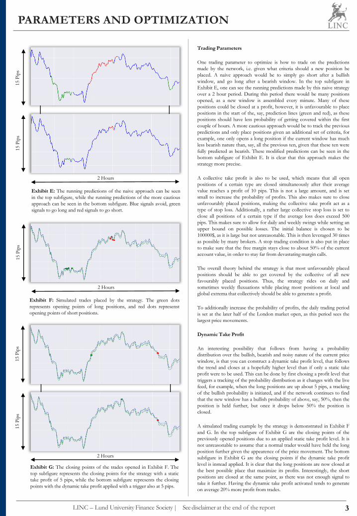
Trading Parameters

One trading parameter to optimize is how to trade on the predictions

made by the network, i.e. given what criteria should a new position be

placed. A naive approach would be to simply go short after a bullish

window, and go long after a bearish window. In the top subfigure in

Exhibit E, one can see the running predictions made by this naive strategy

over a 2 hour period. During this period there would be many positions

opened, as a new window is assembled every minute. Many of these

positions could be closed at a profit, however, it is unfavourable to place

positions in the start of the, say, prediction lines (green and red), as these

positions should have less probability of getting covered within the first

couple of hours. A more cautious approach would be to track the previous

predictions and only place positions given an additional set of criteria, for

example, one only opens a long position if the current window has much

less bearish nature than, say, all the previous ten, given that these ten were

fully predicted as bearish. These modified predictions can be seen in the

bottom subfigure of Exhibit E. It is clear that this approach makes the

strategy more precise.

A collective take profit is also to be used, which means that all open

positions of a certain type are closed simultaneously after their average

value reaches a profit of 10 pips. This is not a large amount, and is set

small to increase the probability of profits. This also makes sure to close

unfavourably placed positions, making the collective take profit act as a

type of stop loss. Additionally, a rather large collective stop loss is set to

close all positions of a certain type if the average loss does exceed 500

pips. This makes sure to allow for daily and weekly swings while setting an

upper bound on possible losses. The initial balance is chosen to be

100000$, as it is large but not unreasonable. This is then leveraged 30 times

as possible by many brokers. A stop trading condition is also put in place

to make sure that the free margin stays close to about 50% of the current

account value, in order to stay far from devastating margin calls.

The overall theory behind the strategy is that most unfavourably placed

positions should be able to get covered by the collective of all new

favourably placed positions. Thus, the strategy rides on daily and

sometimes weekly fluxuations while placing most positions at local and

global extrema that collectively should be able to generate a profit.

To additionally increase the probability of profits, the daily trading period

is set at the later half of the London market open, as this period sees the

largest price movements.

Dynamic Take Profit

An interesting possibility that follows from having a probability

distribution over the bullish, bearish and noisy nature of the current price

window, is that you can construct a dynamic take profit level, that follows

the trend and closes at a hopefully higher level than if only a static take

profit were to be used. This can be done by first chosing a profit level that

triggers a tracking of the probability distribution as it changes with the live

feed, for example, when the long positions are up about 5 pips, a tracking

of the bullish probability is initiated, and if the network continues to find

that the new window has a bullish probability of above, say, 50%, then the

position is held further, but once it drops below 50% the position is

closed.

A simulated trading example by the strategy is demonstrated in Exhibit F

and G. In the top subfigure of Exhibit G are the closing points of the

previously opened positions due to an applied static take profit level. It is

not unreasonable to assume that a normal trader would have held the long

position further given the appearence of the price movement. The bottom

subfigure in Exhibit G are the closing points if the dynamic take profit

level is instead applied. It is clear that the long positions are now closed at

the best possible place that maximize its profits. Interestingly, the short

positions are closed at the same point, as there was not enough signal to

take it further. Having the dynamic take profit activated tends to generate

on average 20% more profit from trades.

Exhibit G: The closing points of the trades opened in Exhibit F. The

top subfigure represents the closing points for the strategy with a static

take profit of 5 pips, while the bottom subfigure represents the closing

points with the dynamic take profit applied with a trigger also at 5 pips.

15

Pip

s

2 Hours

Exhibit E: The running predictions of the naive approach can be seen

in the top subfigure, while the running predictions of the more cautious

approach can be seen in the bottom subfigure. Blue signals avoid, green

signals to go long and red signals to go short.

Exhibit F: Simulated trades placed by the strategy. The green dots

represents opening points of long positions, and red dots represenst

opening points of short positions.

15

Pip

s

2 Hours

15

Pip

s

2 Hours

15

Pip

s15

Pip

s

PERFORMANCE, STATISTICS AND CONCLUSION


Exhibit H: The trading period equity and balance curves. The balance

curve represents the initial value of the account plus the realized profits,

while equity curve represents the balance plus the unrealized profit or

loss. The trading period spans 41 working days from 17th of October to

13th of December.

Total Net Profit 44790$ 29070$ 15720$

Gross Profit 52970$ 35710$ 17260$

Gross Loss -8180$ -6640$ -1540$

Profit Factor 6.5 5.4 11.2

Total Number of Trades 322 184 138

Percent Profitable 86.3% 84.2% 89.1%

Winning Trades 278 155 123

Losing Trades 41 27 14

Even Trades 3 2 1

Avg. Trade Net Profit 140$ 159$ 113$

Avg. Trade Net Loss 191$ 232$ 140$

Largest Winning Trade 1370$ 1370$ 590$

Largest Losing Trade -770$ -770$ 670$

Return on Initial Capital 45.7% 30.7% 15.0%

Annual Rate of Return 291.7% 196% 95.7%

Performance Summary

ShortLongAll

Sharpe

Ratio

Average Daily Return 3.7%

Standard Deviation 4.9%

Max Drawdown 15.6%

12.1Daily Value at Risk 7.6%

Common Metrics

Trading Details

Performance

As can be seen by the balance and equity curves in Exhibit H, the strategy

managed to consistenly collect a rather large profit in just about 41 working

days. This resuls in a return on initial capital of 45.7%, which amounts to

45700$, which includes the profit of about 1575$ made from roll over fees

minus 650$ from transaction fees. This amount of profit was possible due

to the large leverage that was used, which does increase risk, however, the

strategy was at no time close to a margin call, as the usable margin was

always stayed above 40000$. Over the trading period the average price had

shifted downwards by about 160 pips from 1.1530$ to 1.1370$. Therefore,

any investment in short position placed in the beginning of this period and

closed at the end would have made a solid return of about 1.4%. One could

thus expect that short positions should generate more profits, however, as

can be seen in the performance summary below, it is interesting to note that

this strategy made about 70% of its profits from long positions, going

against the major trend of the price. The strategy detected more signals to

go long than it did to go short. This could mean that when the price does

swing against the current major trend, it tends to do so more distinctly than

when the price moving with it. But as expected, and can be seen in the

performance summary, the placed short positions were more likely to be

profitable, having a profit factor of 11.2, while placed long positions had of

profit factor of 5.4, which is still significant.

Statistics

As can also be seen in the performance summary, the average daily return is

quite substantial at 3.7%, also the standard deviation is substantial, this

could be expected as the strategy does carry some positions over to the next

day, even the weekend, therefore, if there is a price gap it would get quite

affected, either posititevly or negatively. Of all long positions 50% were

closed within the first day, while for all short positions it was a significant

80%. The average holding time for all positions is a little more than one

day, with about two weeks being the maximum and one minute the

minimum. The maximum drawdown is 15.6%, this is large but should be

acceptable as the strategy produces a high return. Two of these sizeable

drawdowns happened late October and mid November, afterwards all

drawdowns were significantly smaller. This is likely due to the shift in

average price during this period. In the beginning the shift is rather sharp

and then later levels out, which seems to happen after 20th of November.

This means that unfavourably placed long positions is even more

unfavourable, as a stop trading condition is set at 50% free margin, the

strategy might not have enough capital to place more favourable positions,

with more capital this should be less of a problem. As seen in the equity

curve of Exhibit H, flat parts are weekends, and significant drawdowns tend

to happen afterwards, one could therefore try and limit some risk by closing

as many positions at the end of the week as possible. The daily value at risk

is 7.6%, which means that an investment of 1000$ could expect to lose 76$

every 20th day. This is also not an unreasonable risk given the return. A

quite common measure of risk adjusted returns is the sharpe ratio, which

for this strategy is calculated to be 12.1, which is considered very high. For

this calculation a 90 day T-bill at 2% was used. Additional trading details

can also be found under the performance summary, of which the most

relevant column should be [All] as that takes into account both long and

short positions.

Conclusion

It was certainly possible to make a successful trading strategy that trades by

the use of computer vision, i.e. through artificial eyes. The strategy

indentifies shifts in prices and places positions at peaks and troughs,

maximizing the probability of profits. It managed to generated a significant

return, which comes with some but manageable risk. There are many ways

of trying to reduce the risk, for example, tracking the monthly nature of

price monvements and only trading long or short positions according to it.

Additionally, the strategy does not take news events into account, a

reduction in risk could also be made by making sure to close positions

before certain news events are scheduled to occur. But regardless it seems

like this strategy can be considered quite successful.

Transaction Fees -646$ -368$ -278$

Roll Over Fees 1575$ 2013$ -438$

140000$

100000$

120000$

LINC – Lund University Finance Society |See disclaimer at the end of the report

DISCLAIMERAnsvarsbegränsning

Analyser, dokument och all annan information (Vidare ”analys(en)”) som härrör från LINC Research &

Analysis (”LINC R&A” (LINC är en ideell organisation (organisationsnummer 845002-2259))) är framställt

i informationssyfte och är inte avsett att vara rådgivande. Informationen i analysen ska inte anses vara en

köp/säljrekommendation eller på annat sätt utgöra eller uppmana till en investeringsstrategi.

Informationen i analysen är baserad på källor, uppgifter och personer som LINC R&A bedömer som

tillförlitliga, men LINC R&A kan aldrig garantera riktigheten i informationen. Den framåtblickande

informationen i analysen baseras på subjektiva bedömningar om framtiden, vilka alltid är osäkra och därför

bör användas försiktigt. LINC R&A kan aldrig garantera att prognoser och framåtblickande estimat

kommer att bli uppfyllda. Om ett investeringsbeslut baseras på information från LINC R&A eller person

med koppling till LINC R&A, ska det anses som dessa fattas självständigt av investeraren. LINC R&A

frånsäger sig därmed allt ansvar för eventuell förlust eller skada av vad slag det än må vara som grundar sig

på användandet av analyser, dokument och all annan information som härrör från LINC R&A.

Intressekonflikter och opartiskhet

För att säkerställa LINC R&A:s oberoende har LINC R&A inrättat interna regler. Utöver detta så är alla

personer som skriver för LINC R&A skyldiga att redovisa alla eventuella intressekonflikter. Dessa har

utformats för att säkerställa att KOMMISSIONENS DELEGERADE FÖRORDNING (EU) 2016/958 av

den 9 mars 2016 om komplettering av Europaparlamentets och rådets förordning (EU) nr 596/2014 vad

gäller tekniska standarder för tillsyn för de tekniska villkoren för en objektiv presentation av

investeringsrekommendationer eller annan information som rekommenderar eller föreslår en

investeringsstrategi och för uppgivande av särskilda intressen och intressekonflikter efterlevs.

Om skribent har ett innehav där en intressekonflikt kan anses föreligga, redovisas detta i

informationsmaterialet.

Övrigt

LINC R&A har ej mottagit betalning eller annan ersättning för att göra analysen.

Analysen avses inte att uppdateras.

Upphovsrätt

Denna analys är upphovsrättsskyddad enligt lag och är LINC R&A:s egendom (© LINC R&A 2017).

5

TRADING THROUGH ARTIFICIAL EYES - linclund.com

Documents

Transcript of TRADING THROUGH ARTIFICIAL EYES - linclund.com