Clemson UniversityTigerPrints

All Theses Theses

12-2015

Trade Openness and Income InequalitySarah PolpibulayaClemson University

Follow this and additional works at: https://tigerprints.clemson.edu/all_theses

This Thesis is brought to you for free and open access by the Theses at TigerPrints. It has been accepted for inclusion in All Theses by an authorizedadministrator of TigerPrints. For more information, please contact kokeefe@clemson.edu.

Recommended CitationPolpibulaya, Sarah, "Trade Openness and Income Inequality" (2015). All Theses. 2505.https://tigerprints.clemson.edu/all_theses/2505

TRADE OPENNESS AND INCOME INEQUALITY

A Thesis Presented to

the Graduate School of Clemson University

In Partial Fulfillment of the Requirements for the Degree

Master of Arts Economics

by Sarah Polpibulaya December 2015

Accepted by: Prof. Scott Baier, Committee Chair

ii

ABSTRACT

This paper investigates the impact of trade openness on country’s income distribution or

income inequality on both developing and developed countries during the years 1960-2005. The data

are grouped into 5 year (10 periods) with 86 countries in the sample. Also, I group countries into 8

regions to observe the changes in trade openness and income inequality during the study period.

Using OLS regressions, the results show that increases in trade openness leads to a greater income

inequality in overall countries. By running the regressions separately for developing and developed

countries, the results indicate an interesting fact: while increases in trade openness increases income

inequality in developing countries, it actually decreases income inequality in developed countries

though the result is not significant.

iii

TABLE OF CONTENTS

Page

TITLE PAGE .................................................................................................................................................................... i

ABSTRACT ....................................................................................................................................................................... ii

INTRODUCTION .......................................................................................................................................................... 1

LITERATURE REVIEW ............................................................................................................................................... 4

TRADE OPENNESS AND INCOME INEQUALITY: A PREVIEW OF TODAY RESULTS ................ 13

METHODOLOGY ....................................................................................................................................................... 22

CONCLUSIONS ............................................................................................................................................................ 35

APPENDICES ................................................................................................................................................................ 37

REFERENCES ............................................................................................................................................................... 74

1

INTRODUCTION

Income inequality has long been a concern of many economists and politicians, especially in

the developing and underdeveloped world. In developed countries like the United States income

does not seem to distribute to its population equally as well. Although United States per capita GDP

as of 2014 was $54,629.5 (World Bank data), this does not imply that all people earn this same

amount of income.

I have experienced myself that income does not distribute equally, in fact there is no way

that income will distribute equally even if the country is a communist (there always someone gains

more than the others). While there are many very rich people in Thailand, probably 2-3% of the

whole population, most of the population in Thailand are considered very, very poor and have a

much different quality of life, although cost of living in Thailand are much lower as compare to the

United States. Apart from that, only 10% of the population of Thailand are considered middle-

income earners and normally are the taxpayer group, but that percentage is seen to be lower each

year (probably the same as the United States).

There are many factors that contribute to greater income inequality in a country or between

countries in the world; nevertheless, in this paper I investigate income inequality that is correlated by

the effects of international trade or globalization. As countries increase in trade, there are both good

and bad sides that may impact population of that country, and one of the bad side is widening in

income gap or greater income inequality in that country. The income gap between skilled and

unskilled labor is also widening, hence, leads to income inequality.

In addition, in this paper I investigate the impact of trade in each region by grouping sample

countries into 8 regions that are: East Asia Pacific, Europe & Central Eurasia, Middle East & North

Africa, South Asia, Western Europe, North America, Sub-Saharan Africa, and Latin America &

Caribbean to observe income inequality among each region though the results may not be very

appreciable due to lack of countries’ data and I did not use all the countries in the world, only 86

2

countries have been observed here in this paper. Obviously, there are many other characteristics of a

country that leads to a different in income distribution whether government policy, quality of life of

the people, how the government weighs the importance of trade (either more export or import), cost

of living, and countries’ minimum wage also have an impact as well.

Developed countries may seem to gain more from trade as they possess technology, large

pool of skilled labor, have a better government (which leads to better trade policy), and also goods

that they export are higher in value than what developing countries export, hence, developed

countries terms of trade (as known as price of exported goods divided by price of imported goods) is

much higher than developing countries. Another way to look is that developed countries have a

lower opportunity cost of trade in terms of exporting expensive or skilled-intensive goods than

developing countries, therefore, they earn more or benefits more as developed countries will likely

import labor-intensive goods or goods that is cheaper. As a result of this, developed countries as they

export skilled-intensive goods (lower cost for producing), demand for skilled labor will increase

which leads to a rise in the wage of skilled labor. On the other hand, labor-intensive goods,

developed countries will import from developing countries, therefore, local firms in that sector may

shut down as they cannot compete with foreign firms (from developing and underdeveloped

countries) which leads to unemployment and demand for unskilled labor in developed countries

decrease and leads to a lower wage for unskilled labor. Therefore, skilled labor in developed countries

will gain and the wage gap in those countries becomes widen resulting in income inequality. On the

other hand, developing (and underdeveloped) countries are more likely to export labor-intensive

goods (due to lower opportunity cost of producing it). This increases the demand for unskilled labor

that leads to a rise in wage for unskilled labor; hence, the income gap in these countries should be

narrower.

Another importance source that trade causes income inequality is through outsourcing,

where firms send to aboard the least skilled and labor-intensive activities and keep only the most

3

skilled and labor-intensive activities at the local. This is done when firms take into account the trade

costs from outsourcing with the lower labor cost due to lower wage rate in foreign countries, which

are underdeveloped and developing countries. By doing so, the relative demand for skilled labor in

those home countries (i.e. developed countries) will increase leads to a rise in relative wage of skilled

labor at home. On the other hand, in the foreign countries (underdeveloped and developing

countries), as developed countries offshore their least skilled and labor-intensive activities, these new

activities become more skilled and labor-intensive than the current activities. Hence, the relative

demand for skilled labor in foreign countries also increases so as the relative wage of skilled labor.

Therefore, both home and foreign countries face a higher relative wage of skilled labor due to the

offshoring that leads to a higher wage gap between skilled and unskilled labor, hence, increase in

inequality in both countries. This implies that income inequality would increase in both developed

and developing (and underdeveloped) world. In addition, skilled-biased technological change is also

one of the reasons for an increase in relative demand for skilled workers that, in turn, leads to a

higher wage gap and causes income inequality within a country but this is beyond the scope of this

paper.

Additionally, Spilimbergo, Londono, and Szehely (1999) find that land- and capital-intensive

countries have higher income inequality, on average, than skilled-intensive countries; therefore, they

conclude that the effect of trade openness on income inequality depends on factor endowments of

each country. As we may be aware that developed countries which mostly are skilled-intensive

countries tend to have a lower income inequality, that is lower GINI coefficient, as compare to

developing countries whereas underdeveloped countries that likely are land-intensive countries tend

to have higher income inequality or higher GINI coefficient.

I investigate the impact of trade on income inequality and also investigate if the impact

differs between developing (and underdeveloped) and developed countries. My hypothesis is that

trade openness leads to a greater income inequality in overall countries and when investigate

4

separately, developing (and underdeveloped) countries and developed countries, trade openness leads

to a greater income inequality in both worlds with a lower rate among developed countries as

according to offshoring model of Feenstra & Hansan which predicts an increases in skill premium in

both developing and developed worlds, and also predicts a rise in a relative skilled workers to

unskilled, therefore this will harm unskilled labor in both economies but should effect developing

and underdeveloped countries more as they are unskilled labor-abundant countries, hence, income

inequality should be worse than those developed countries. Although there are several papers that

study the impact of trade on income inequality, it is of my interest in terms of economic study;

therefore, I compile things that past studies propose so far but using different data set, different time

period, and different investigating methods. As a matter of fact that I have limited scope of

education, I try to utilize everything I have studied or learned so far to conduct this thesis research

paper.

LITERATURE REVIEW

There are several papers that have investigated the impact of international trade on income

inequality. Accordingly, I limit the literature review to selected empirical papers and summarize the

main findings that related and provide interesting results, however, it would be better to begin with

the discussion of simple 2-by-2 models of international trade.

Starting with the Ricardian model with labor as a single factor of production, the level of

productivity times the price of the good determines the wage rate. Therefore, wages are determined

by country’s absolute advantage. In other words, countries with better technology are capable of

paying a higher wage seeing that they are able to produce more. Also, wage depends upon the price

of the good that the country exported, which depends on the world market. Hence, country’s terms

of trade (price of exported goods divided by price of imported goods) comes to a play as country

with higher terms of trade, meaning that it has a high exported price, the real wages of that country

5

also high, and therefore benefit the workers. This may be the case that developed countries as they

have higher productivity together with better technology than developing (and developed) countries,

price of the their exported goods will be higher therefore, they have a higher wage rate as well. In this

model, countries will want to produce only the goods that they are specialized in producing and

export them. Therefore, labor demand in export sector will be higher and resulting in higher wage

rates. In contrast, the opposite impact is found in import. As a consequence, exports sector will

benefit while import sector will loss, therefore, increase in inequality within the country.

Next, the Heckscher-Ohlin Model which assumes that trade occurs due primarily to

different factor endowmenrs as contrast to Ricardian model which assumes countries trade because

they use their technological comparative advantage to specialize in production of different goods1.

Moreover, the model predicts that the real gains go to the factor used most intensively in the export

goods whose relative price goes up when country opening to trade and the loss goes to the other

factor or import sector. However, this model assumes that a country has only two factors of

production that can be mobilized between sectors with the same technology across countries. As

developed countries are skilled labor-abundant countries, that is, they exports skilled-intensive goods,

relative wage rate of skilled labor increase widens the wage gap, hence, leads to greater income

inequality in the developed countries. On the contrary, developing and underdeveloped countries as

they are seen as unskilled or low skill labor-abundant countries, they export goods that are unskilled

or low skill-intensive goods. Hence, relative wage rate of unskilled or low skill labor go up, resulting

in narrower wage gap in the country, which in turn lower income inequality within developing and

underdeveloped countries.

Another factor that leads to greater income inequality in the country is outsourcing of which

a country outsource the least skilled-intensive activities to the country that required lower labor wage

in order to lower the cost. As, for example, developed countries outsource activities which require

1  Feenstra, R. C., Taylor, A. M. 2014.“International Trade” 3rd Edition. Worth Macmillan.

6

the least skilled to the developing and underdeveloped countries, hence, they left only skilled job in

the country whereas low-skilled or unskilled labor will loss their jobs resulting in greater inequality

within the country. In addition, these least skilled-intensive goods now become skilled-intensive

goods in developing countries; therefore, relative demand for skilled labor increase so as the relative

wage rate of skilled labor, hence, leads to a widening of the distribution of income in the country as

well. Feenstra and Hanson’s model of offshoring expects that as countries outsource, the relative

wage rate of skilled labor rise in both developed and developing countries. In addition, the ratio of

skilled to unskilled labor increases in both developed and developing worlds as well. Thus, leading to

a widening of income distribution in both developed and developing countries.

Branko Milanovic (2006) summarized the debate on the measurement and implications of

global inequality among countries as well as investigated the relationship between globalization and

global inequality to show why it is matters. The author asserted that to calculate global inequality,

data on national income distribution for most of the countries in the world, or at least for most of

the populous and rich countries is needed, therefore, the first estimation of inequality among

countries were done in the early 1980s. Also, it is then when the data for income distribution were

accessible for China, Soviet Union and its constituent republics, and large parts of Africa. The author

delineated 3 concepts of inequality. First: inequality among countries’ mean incomes or inter-country

inequality (dubbed by Milanovic, 2005). This first concept has only little to tell about income

inequality among countries due to the difference in population size. Second: inequality among

countries’ mean incomes weighted by countries’ populations. This concept requires only two

variables that is mean income (preferably in per capita) and population size, hence, it is popular as it

is the largest component of global inequality and can be used as a lower-bound proxy for global

inequality as well as track the changes but this concept does not take into account within-country

inequalities as it assumes that each individual in a specific country has the same per capita income.

Third: inequality between the world’s individual or global, this last concept must be based on

7

household surveys but there is no world-wide household survey, therefore, the best we could do is to

combine each country’s survey and use disposable per capita income or personal per capita

consumption as a welfare indicator. Milanovic (2006) focused on the studies of global or concept 3

income inequality (last concept). The way to estimate this is to calculate concept 2 inequality using

nation accounts data and the only additional data needed is the GINI coefficient or some other

summary inequality statistic indicating national income distribution. The methods require very little

information but are costly as there are several assumptions that needed to be made that may drive the

results. GINI data is also not always available annually and this leads to additional empirical issues.

Therefore, imputed data as a selected sample may result in biased estimate. Milanovic (2006) suggests

that the income distribution data, especially when extrapolated from GINI coefficients, contains lots

of noise; also, due to the absence of income distribution data for many countries, several authors

assert questionable assumptions, for example, income distributions do not change overtime or

change in a certain fashions or even everyone in the country has the same income, which seems

unreal. Milanovic also investigated the linkage between globalization and global inequality. The

author claims that the casual linkage is not immediately obvious; as there are many ways that

globalization may affect countries’ inequalities. First, the effects on within-country distributions,

according to Hecksher-Ohlin theory, globalization is supposed to increase the demand and wages for

unskilled labor in poor countries as well as increase the wage of skilled labor in rich countries and, as

a result, we would expect that income distribution in poor countries to be improved and in rich

countries to be worse. But for the past twenty years it has been seen that the income distributions

among poor, middle-income, and rich countries grow even more unequal, which is inconsistent with

what is predicted by Hecksher-Ohlin theory (Cornia and Kiiski 2001). Secondly, globalization may

affect mean incomes in poor and rich countries differently and there is still no conclusion on this

matter. Most authors claim that trade openness leads to mean income growth but some found that

the affect is stronger in poor countries (Sachs and Warner 1997; World Bank 2002), while some

8

claimed that the affect is seen to be larger for rich countries especially during these past twenty years

(DeLong and Dowrick 2003; Dowrick and Golley 2004). Thirdly, the effects of globalization may

differ amongst populous and small countries but there still little investigation in this matter. Lastly

and interestingly, the effect of globalization on global inequality is seen to depend on countries’

history as to whether populous countries were rich or poor at a particular point in time. If the

populous countries are poor, globalization on average benefits small countries and leads to the

widening of national income distributions; hence, the overall effect is a rising in global inequality.

Therefore, the author concluded that all statements about the relationship between globalization and

global inequality are highly depend on time-specific conditional on countries’ past income history.

Kahai and Simmons (2005) used GINI coefficient as a measure of inequality to explore the

linkages with globalization. For developing countries, they found that globalization is positively

associated with an increase in income inequality but for overall countries their results indicate that

worsening of the globalization index or lower trade openness is associated with an increase in income

inequality.

Anderson (2005) showed that increased openness of trade affects income inequalities within

developing countries by affecting asset, spatial, and gender inequalities as well as the amount of

income distribution.

Dollar and Kraay (2001) studied the effect of globalization on inequality and poverty and

found a strong positive effect of trade on growth. Moreover, the increase in growth rate that goes

along with an expanded trade leads to a proportionate increase in income of the poor, and therefore,

they concluded that globalization leads to a faster growth and a poverty reduction in poor countries.

Duncan (2000) also found a strong association between economic growth and the reduction of

absolute poverty.

Calderon and Chong (2011) showed that the intensity of capital controls, exchange rate, type

of exports, and the volume of trade affect the long run distribution of income. They grouped the

9

data into 5 year intervals then averages for periods between 1960 – 1995 and found that trade

reduces income inequality. In addition, Ghose (2001) used 96 countries over 16 year periods (1981-

1997) and found that inter-country inequality has been growing whereas international inequality has

been declining at the same time.

Cornia (2003) examined the changes in global between country and within-country inequality

over the years 1980-2000 and found that within-country inequality has risen clearly in two-thirds of

the 73 countries that have been investigated due to policy driven towards domestic deregulation and

external liberalization.

Spilimbergo, Londono, and Szekely (1999) investigated the empirical links between factor

endowments, trade, and personal income distribution. Their result showed that land and capital-

intensive countries have a less equal income distribution whereas skilled-intensive countries show a

more equal income distribution. As a result, they concluded that effect of trade openness on income

inequality depends on factor endowments. This is an interesting investigation by focusing on factor

endowments, which I will not investigate in this research paper.

Amerlia U. Santos-Paulino, “Trade, Income Distribution and Poverty in Developing

Countries: A Survey” (2012), investigated how trade and trade liberalization affect poverty and

income distribution. The paper shows that poverty impediment originates from various sources

including infrastructure, skills, incomplete markets, and policies. It investigates the theoretical and

empirical research on how trade openness affects poverty and inequality focusing on developing

economies. Empirical results show that poor countries tend to face greater barriers on their exports

than those of advance countries (Looi Kee et al., 2009). It also suggested that increased inequality is

seen to be acceptable if it comes along with a sustainable growth, and as a result, although there is a

rise in income disparities, the poor will still be better off in absolute sense. Moreover, it is to be

expected that trade liberalization will rise relative wages of unskilled workers and could as well

worsen income distribution as it might encourage the promotion of skill-biased technical change in

10

response to increase in foreign competition, or to increased globalization of production (Feenstra,

2008). Empirical evidence suggests that trade liberalization is unlikely to produce beneficial results

across all countries or households. In addition, studies focusing on trends of income distribution are

also conflicting to each other as some show a reduction in global inequality while others show that

inequality still remains uncontrollable.

UNCTAD’s LDCs report in 2004 found that there was a high tendency for poverty in Least

Developed Countries (LDCs) with the most open to trade and lower poverty for LDCs that

liberalized their trade more slowly. In addition, changes in per capita income are seen to be the main

determinants for changes in poverty as well. For example, if open more to trade leads to faster

growth in incomes and if that growth increases the income of the poor equivalently, absolute poverty

will be reduced. On the other hand, economic growth also has consequences on income distribution

as well as poverty. Kanbur 2010; Nissanke and Thorbeche 2010, found that there is a significant

tradeoff between poverty and inequality as economic growth leads to a reduction in poverty, it could

as well increase inequality. Basu (2006) suggested that changes in per capita income are the main

determinants in changes in poverty but maximize per capita income during globalization period

might not take into account poverty problem and inequality reduction. Inequality is seen to be one of

the most significant impacts from globalization in the same way that economic growth impacts

income distribution and poverty.

Paulino (2012) claimed that if trade liberalization widens the income distribution, it would

not lead to poverty reduction though it leads to positive economic growth. Goldberg and Parnich

(2007b) found a contemporaneous increase in globalization along with inequality in most developing

countries; hence, they suggested that countries’ policies should be examined as well. Dowrich and

Gulley (2004) showed that benefits of trade mostly go to richer economies with less benefits to less

developed countries and that the dynamic benefits of trade come from productivity growth. The

evidence suggests that the faster the countries grow the faster the poverty rate will fall, also, in LDCs,

11

higher growth leads to a lower poverty rate. Trade openness could lead to faster growth in average

income and if that growth, in turn, increases incomes of the poor “proportionately”, it will lead to a

decreased in absolute poverty but the evidences and arguments on that effect are still inconclusive

especially in the case for LDCs. There is still no verification that trade openness will lead to increase

in growth that, in turn, will lower the poverty rate. UNCTAD 2004:77 claimed that the relationship

between trade openness and poverty is conditional on the level of development of the country as

well as the structure of its economy and its exports. For now, it is still implausible to identify the way

in which per capita GDP (as a measure for development) affects the influence of openness on

inequality. Case studies in many countries show that trade openness leads to economic growth that,

in turn, reduce poverty rate and foster the development of a country, nevertheless, the paper suggests

that on average these studies did not seem to represent the reality of specific countries or regions

which lead to significant upward or downward bias results. In the conclusion part, Paulino (2012),

found that trade openness correlated with other reform areas as well particularly in the quality of the

institutions, that is, the rule of law, corruption, effective government, and political instability (Rodrik,

2001). Additionally, Winter (2004) argues that trade liberalization by itself is unlikely to boost

economic growth unless the openness improves institutional stances of a country (i.e. reduce

corruption and rent seeking). Paulino (2012) also claimed that it has been predicted that global

economic integration should help the poor since poor countries have comparative advantage in

producing good intensive on unskilled labor. Studies tend to advocate that trade openness improves

overall welfare but the benefits are unequally distributed. Welfare is measured by change in price, the

relative demand for domestic factors of production, and demand for skilled relative to unskilled

labor. Moreover, trade policy is seen to play a vital role on distributional impacts, especially in low-

income countries and LDCs. The main issue here is the protections, such as taxes and benefits, and

how will it affect the poor. In addition, the paper suggested that the main cause of poverty could be

due to the loss of employment and unemployment, therefore, policy makers need to be concerned on

12

this issue (employment effect) as well. The effect of trade on employment (whether income or price

of goods) tends to be one of the major causes of inequality but in this research paper I will not focus

on this factor even so this literature tends to explain other sources that increase income inequality

through trade and provides more perspective in the area.

In “Impact of International Trade on Income and Income Inequality”, Aradhyula, Rahman,

and Seenivasan (2007): their estimation strongly involves using an error component two-stage least

square random effects IV regression model (EC2SLS) followed Baltagi (2005). This specification is

closest to the model employed in this paper. The paper followed the work of Frankel-Romer (1991),

Irwin-Teruio (2002) and Noguer-Siscart (2003) which included geographic characteristics, as they are

highly correlated with trade and uncorrelated with income as well as using geographic characteristics

as the instrument to study the impact of trade on income. This paper uses trade openness instead of

total trade as an indicator for international trade and uses geographic area and countries population

as an instrument for trade openness with an intuition that countries with larger area and population

tend to have lower trade openness than the smaller countries. The idea behind the model for

studying the impact of trade on income inequality is to regress the log of GINI index on log of trade,

dummies for landlockedness, democracy index, corruption index, and dummy for developed

countries. Using Pooled OLS technique trade is an endogenous variable that is likely correlated with

the error term and result in biased in the parameters estimates. They constructed instrument by

regressed log of trade openness on geographic area and countries population as well as other

variables, then they predicted the values to be used in the second stage regression by substituting it

with trade openness and estimated using EC2SLS procedure. For the first stage regression, the result

shows that geographic area and countries population are significant variables in explaining trade.

While democracy index was also significant they didn’t use it as an instrument because it might affect

both trade and income inequality. In the second stage, the result shows that trade openness has a

positive significant impact on income inequality. A 1% increases in trade openness increases income

13

inequality by approximately 0.14% at a 1% significant level but the magnitude of the increases in

income inequality seems to be lesser in developed countries (approximately lower by 0.3041

percentage point). They also suggested that trade increases income with democracy has a positive

influence on it as well as on income inequality since upper and middle income groups increase far

more than the lower income group in democratic countries. Additionally, by dividing countries into

developed countries and developing countries, they found that trade openness reduces income

inequality in developed countries, though not significant, in contrast to developing and

underdeveloped countries which trade openness increases income inequality by approximately

0.1920% at a 1% significant level. For the overall results, they concluded that trade openness

increases both income and income inequality in overall countries.

Trade Openness and Income Inequality: A Preview of Today Results

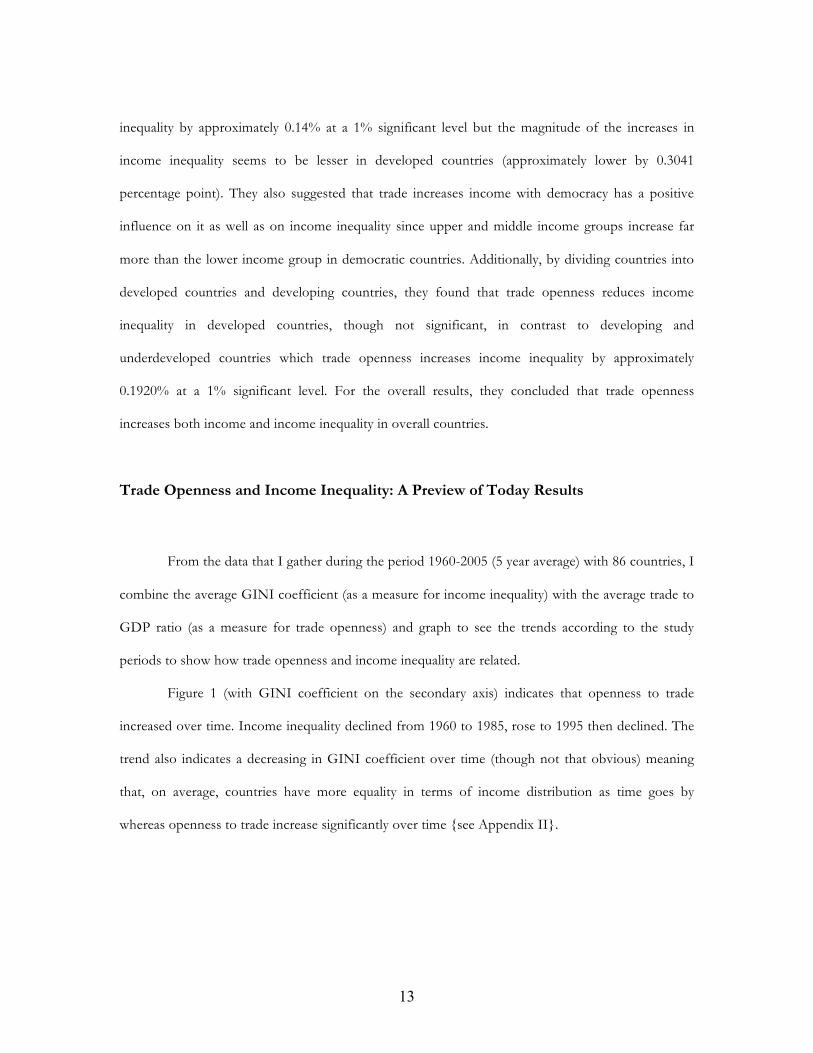
From the data that I gather during the period 1960-2005 (5 year average) with 86 countries, I

combine the average GINI coefficient (as a measure for income inequality) with the average trade to

GDP ratio (as a measure for trade openness) and graph to see the trends according to the study

periods to show how trade openness and income inequality are related.

Figure 1 (with GINI coefficient on the secondary axis) indicates that openness to trade

increased over time. Income inequality declined from 1960 to 1985, rose to 1995 then declined. The

trend also indicates a decreasing in GINI coefficient over time (though not that obvious) meaning

that, on average, countries have more equality in terms of income distribution as time goes by

whereas openness to trade increase significantly over time {see Appendix II}.

14

Figure 1: Trade Openness and Income Inequality

It may be useful to investigate the relationship between openness and inequality by regions

as well. I use 8 regions (followed by Wikipedia website); East Asia Pacific, Europe & Central Eurasia,

Middle East & North Africa, South Asia, Western Europe, North America, Sub-Saharan Africa, and

Latin America & Caribbean (see Appendix I for list of countries by region). I used a population

weighted average as well in order to account for the size of a country, then combined weighted

average GINI coefficient with weighted average trade to GDP ratio and graphed to see the trends

according to the study periods to show how trade openness and GINI coefficient related in each

region (note that GINI coefficient is on the secondary axis for all figures).

East Asia Pacific: Figure 2 shows that trade openness increased overtime started from 1965 while

GINI coefficient exhibited no dissembles patterns for this set of countries.

15

Figure 2: Trade openness and Income Inequality in East Asia Pacific

Europe & Central Eurasia: Figure 3 depicts that overall trends for both GINI coefficient and trade

openness are increasing. During 1960-1970 (3 periods), trade openness increase significantly while

GINI coefficient tended to fall as during these periods we have only one developed country

(Hungary), hence, after adding additional country trade openness declined and GINI started to rise

up. Starting in 1990, with more countries incorporated into this region the graph should contain

more information. Trade openness increased, as did the GINI coefficient that started to stabilize

since 1995 with a small drop (less than 1 point) during 2000-2005.

16

Figure 3: Trade openness and Income Inequality in Europe & Central Eurasia

Middle East & North Africa: For this region, Figure 4 shows from 1960-1970, both trade

openness and GINI coefficient increased significantly. After 1970 GINI coefficient started to decline

whereas trade openness increased until 1985, when it started to fall along with GINI coefficient. This

is because I added another country from year 1990 that is Egypt, which accounted for the most

population weight in this region with mediocre trade openness and low GINI coefficient as compare

to other countries in the region, hence, both overall trade openness and overall GINI coefficient

decreased. But the period 1995-2000, GINI coefficient shows a rise as Egypt had a significant

increase in its GINI coefficient. During 2000-2005, Trade openness shows a sharp increase while

GINI coefficient indicates a fall, this is due to Egypt had a remarkable increase in its trade openness

and all sample countries had a lower GINI coefficient.

17

Figure 4: Trade openness and Income Inequality in Middle East & North Africa

South Asia: Figure 5 shows that starting in 1965 trade openness increased dramatically while GINI

coefficient showed almost no movement with the exception of 1960, 1970, and 2005. But then India

had a sharp drop in its GINI coefficient in year 1980, hence, the overall GINI coefficient dropped

again and remained stable afterward with an increasing trend in 2000-2005 on account of India. For

overall trade openness, it shows a small drop during period 1980-1985 as all countries in the sample

had lower trade openness but then it started to rise again afterward (all countries show a higher

openness).

18

Figure 5: Trade openness and Income Inequality in South Asia

Western Europe: Figure 6 - In this region all the countries in the sample are developed countries.

There is a small drop in trade openness during 1985-1990 as most of the countries in this region

faced a decrease in its trade to GDP ratio but then it started to rise back up afterward with a sharp

rise during 1995-2000 as Germany, which accounts for the most population in this region had a

significant increase in its trade to GDP ratio. The overall trend indicates that trade does benefit

developed countries in terms of better distribution of income but it is not appropriate to conclude

right away.

19

Figure 6: Trade openness and Income Inequality in Western Europe

North America: For this region we have only two countries as a sample that are Canada and United

States, therefore, the result may not be reliable to conclude for the whole region. Figure 7 shows that

the overall trend indicates an increasing in trade openness over time. For GINI coefficient, the trend

shows somewhat stable with a rise during 2000 to 2005. In 2005, I have only United States as a

sample; hence, the graph shows a rise in GINI coefficient along with a drop in trade openness as

United States has a much larger economy (higher GDP) than Canada as a result it had a lower trade

to GDP ratio. United States also has a higher GINI coefficient.

20

Figure 7: Trade openness and Income Inequality in North America

Sub-Saharan Africa: This region possessed the highest GINI coefficient of all the regions that I

have studied so far. From Figure 8, as we look at period started from 1985 it shows an increasing

trend in trade to GDP ratio along with a declining trend in GINI coefficient, therefore, open to trade

leads to a better income distribution in this region after the year 1985. The graph shows a sharp drop

in openness to trade in the period 1965-1970 particularly due to in 1970 I added two more countries

that have low trade to GDP ratio and also accounted for most of the population weight that is

Nigeria, hence, the overall average trade openness drop but it started to rise again after that as all

countries have a higher trade to GDP ratio. For GINI coefficient, it shows a drop during 1970-1975

as almost all countries in the sample had a drop in its GINI especially Nigeria that had a significant

drop. The GINI coefficient started to rise again until 1990 as I had more countries in the sample

after that it show a declining trend over time.

21

Figure 8: Trade openness and Income Inequality in Sub-Saharan Africa

Latin America & Caribbean: Figure 9 shows that this region open more to trade over time but its

GINI coefficient remained quite stable (around 50 points) meaning that distribution of income

(equality of income) does not improve as countries in this region open more to trade. All countries in

my sample for this region are developing countries and this graph shows what several papers have

found as their result that openness to trade leads to increase in income inequality, here we used GINI

coefficient as a measurement, in developing countries (Kahai and Simmons 2005, Anderson 2005,

and Aradhyula, Rahman, and Seenivasan 2007).

22

Figure 9: Trade openness and Income Inequality in Latin America & Caribbean

From all the figures (graphs) above, I found that for some regions, the graph shows as what

could have been expected while some indicate insignificant relationship between trade openness and

income inequality as used GINI coefficient for measurement, therefore, I investigate further with

regression analysis along with other explanatory variables to observe whether open more to trade

leads to worsening in income distribution (increases in income inequality) or not.

METHODOLOGY

To investigate the impact of trade openness on the distribution of income within a country, I

use a panel technique. However, we do not have observations for all countries in each time period so

we have an unbalanced panel.

Data

The panel includes the measures of trade to GDP ratio and countries’ GINI coefficient as

well as other control variables discussed below. There are 86 countries covering the years 1960-2005,

23

of which I averaged the data into 5 years (10 periods total). My sample of countries contains both

developed and developing countries, and the data are drawn from various sources including World

Bank and CIA websites.

The dependent variable is the GINI coefficient as the measure of income inequality within

the country. Explanatory variables include: trade openness; per capita GDP of each country in the

sample; black market exchange rate that is the rate per one US dollar; longitude of the countries;

latitude of the countries; geographic areas of the countries; country’s life expectancy; and country’s

terms of trade.

Following the study of Aradhyula, Rahman, and Seenivasan (2007), I use GINI coefficient as

a measurement for income inequality within a country. The GINI coefficient (also known as the

GINI index or GINI ratio) is a measure of statistical dispersion intended to represent the income

distribution of a nation's residents, and is the most commonly used measure of inequality. The GINI

coefficient measures the inequality among values of a frequency distribution (for example, levels of

income). A GINI coefficient of zero expresses perfect equality, where all values are the same (for

example, where everyone has the same income). A GINI coefficient of one (or 100%) expresses

maximal inequality among values (for example, where only one person has all the income or

consumption, and all others have none)2.

For the measurement of a country’s openness to trade I use trade to GDP ratio following

previous studies. Per capita GDP of sample countries included as a measure for development due to

the fact that more development countries tend to have lower inequality. Countries’ longitude and

latitude are included as a proxy for institutional quality (Hall and Jones (1999)) as most of the

countries with high latitude degrees were mostly conquered by the Europeans, which are seen as

2  https://en.wikipedia.org/wiki/Gini_coefficient  

24

bringing good quality institution along with them3. Area also included into the model as a control for

size of a country as a larger economy tends to distribute their income among citizens more difficult.

Life expectancy is included as a proxy for poverty as countries with bad healthcare system, that is,

low life expectancy rate are usually poor countries with high inequality. Terms of trade, that is the

amount of imports goods an economy can purchase per unit of export goods, also included as

countries will benefit with high terms of trade as they can purchase more imports goods for any

given level of exports4, hence, countries’ inequality should be lower as they will gain more from trade.

Black market exchange rate included as a control variable as it has an impact on income distribution

as well through country’s factor endowments5.

3  Aradhyula, S., Rahman, T,. and Seenivasan, K. 2007. Impact of International Trade on Income and Income Inequality. Selected paper for presentation at the American Agricultural Economics Association Annual meeting in Portland, OR  4  https://en.wikipedia.org/wiki/Terms of trade  5  Pablo García Silva. 1999. Income Inequality and the Real Exchange Rate. Central Bank of Chile Working paper. No.54.    

25

Descriptive Statistics

Table I lists the summary statistics for the variables used in the empirical specification.

Table I: Definitions and descriptive statistics of variables used in the model

Variable Definition Mean Std Dev Min Max gini Gini coefficient:

Measurement for income inequality expressed in % with 0% expresses perfect equality and 100% expresses maximal inequality

39.0564 10.32915 17.65 70

tradegdp Trade to GDP ratio: Measurement for trade openness that is amount of export and import divided by GDP

68.97054 45.29316 7.75584 444.315

Log (tradegdp) Log of Trade to GDP ratio

4.048052 0.6279389 2.048446 6.096534

exportsgd Export to GDP ratio 33.21652 23.62349 2.85908 236.445

Log (exportsgdp) Log of Export to GDP ratio

3.294175 0.6662562 1.063013 5.465716

importsgdp Import to GDP ratio 35.75403 22.4641 3.92657 207.87

Log (importsgdp) Log of Import to GDP ratio

3.395343 0.6266518 1.367766 5.336913

gdp_pc GDP per capita expressed in dollar terms

11659.56 10021.21 621.548 71209.3

Log (gdppc) Log of GDP per capita 8.952363 0.9803252 6.432213 11.17338

black_mkt_er Black market exchange rate per one dollar

68.39911 759.6582 -23.28 139000

longitude Longitude of countries measured in degrees

14.23275 67.37052 -118.21 174.78

latitude Latitude of countries measured in degrees

23.37228 27.27049 -36.892 60.212

area Area of countries measured in Sq.Km.

202591.5 237222.5 439.9 977956

life_exp Life expectency measued in years

68.45841 8.373465 40.4737 81.0761

terms_of_trade Countries' terms of trade that is price of country's exported goods divided by price of country's imported goods

-3.72E+11

7.49E+12

-8.4E+13

4.7E+13

26

The GINI coefficient has a mean of 39.05% with a minimum of 17.65% and a maximum of

70%, hence, there is a wide range of measures for the distribution of income across countries in the

sample. Openness to trade shows a minimum of 7.76% with a maximum of 444.32%, the mean is

68.97%. Some countries are more open to trade than others. Generally speaking large countries tend

to trade a smaller share of their GDP, for example, countries like United States and Japan tend to

have a lower trade to GDP ratio than a small country such as Singapore. The mean of exports share

of GDP is 33.22% with a minimum of 2.86% and a maximum of 236.45%, while share of imports

shows a mean of 35.75% with a minimum of 3.93% and a maximum of 207.87%. For per capita

GDP, the mean of all 86 countries are $11,659.56 with a minimum as low as $621.55 to a maximum

of $71,209.30. We can notice the large differences between the rich and the poor countries, which

indicate a large variability in income among countries in the sample. Another important variable is

the life expectancy; the mean for all countries of 68.5 years with a minimum of 40.5 years to a

maximum of 81 years, therefore, the well being of people (health) is also not equal among all

countries in the sample. Moreover, the value of terms of trade as shown are quite large as, according

to the World Bank data, it is a terms of trade adjustment and is in a constant local currency. It is

equal to capacity to imports less exports of goods and services in constant price. Other control

variables’ statistics are shown in the same table.

In addition, I go through average GINI coefficient in each region during 1960-2005 and

then do weighted average GINI coefficient that I weighted each country by its population size than

average for each region as well. After that I will investigate trade to GDP ratio, which I use as a

measure for trade openness, I do both simple average and weighted each country by its population

size for each region {see Appendix III}.

27

Model Specifications

Aradhyula, Rahman, and Seenivasan (2007), which did a similar study used error component

two-stage least square random effects IV regression model (EC2SLS) as they found that trade is an

endogenous variable that will be correlated with the error term, hence, the estimators are biased. To

counter this problem, they used area and population of the countries as an instrument for trade, then

use EC2SLS regression model to study the impact of trade on income inequality. The model that

they use is quite similar but is different in many aspects. While they used the data from 1984 to 1996

with 44 countries, I grouped the data into 5-year averages for the period 1960 to 2005. The

explanatory variables used to control in the model are also different. In addition, I use OLS

regression analysis to study the impact of trade openness on income inequality as after I tested for

endogeneity of trade to GDP ratio the result shows that it is not an endogenous variable in my case,

therefore, I did not conduct an instrument variable as the paper describe above did. My basic model

1 is:

GINIi,t = α + β1Log (trade to GDP)i,t + β2lagged changes Log(per capita GDP)i,t + β3Black market exchange ratei,t +

β4Longitudei + β5Latitudei + β6Areai + β7Life expectancy + β8Terms of tradei,t + εi,t

I expected to see β1> 0 as I believe that increase in trade openness is one reason for an increase in

income inequality, especially in developing countries, where α represents vertical intercept and εi,t is a

stochastic error term for country i at time t.

Empirical Results

I regressed GINI coefficient on log of trade to GDP ratio; lagged changes in log per capita

GDP; black market exchange rate; longitude; latitude; area; life expectancy, and terms of trade. The

results show that all variables are significant at 1% level. The results are shown in table IIA below.

28

Table IIA: Regression parameter estimates using Trade to GDP ratio

Variable name Parameter Estimate Standard Errors Test Statistics p-value Constant 70.91214 4.801555** 14.77 0.000

Log of trade to GDP ratio 2.124265 0.8010208** 2.65 0.009

Lagged changes in log of per capita GDP

15.11229 4.159617** 3.63 0.000

Black market exchange rate -0.0344615 0.0130564** -2.64 0.009

Longitude -0.0579235 0.0066114** -8.76 0.000

Latitude -0.1716282 0.0169992** -10.10 0.000

Area 9.13E-06 2.01E-06** 4.55 0.000

Life expectancy -0.5620107 0.0635353** -8.85 0.000

Terms of trade 1.52E-13 5.09E-14** 2.99 0.003

R-squared 0.5953      Number of Observations 216      

Dependent variable: GINI coefficient ** Indicates statistical significance at 1% level

The results of the model (Table IIA) show that openness to trade does have a positive

impact on income inequality (β1> 0). A 1% increase in trade to GDP ratio (openness to trade) leads

to an increase in income inequality (GINI coefficient) by 2.12 points, hence, open more to trade

leads to increases in country’s income inequality and this coefficient is statistically significant at 1%

level. This result is consistent with past studies such as Aradhyula, Rahman, and Seenivasan (2007)

that found that a 1 % increases in trade openness increases income inequality by 0.14% at 1%

significance level, Kahai and Simon (2005), and Anderson (2005) as well as the theoretical model of

Feenstra (1997) that predicted that more trade openness leads to increase in income inequality in

overall countries.

The coefficient on lagged changes in log of per capita GDP is positive due to the fact that

increase in per capita GDP does not imply that everyone is made better off an increase in it can

accompany income inequality. The coefficient on black market exchange rate is negative as if country

currency appreciation (can exchange for more dollars per their local currency) that country should be

better off (less inequality compare to other countries). The coefficient on longitude and latitude are

29

both negative as well due to the fact that country with high latitude and longitude degrees usually

have better institution, developed from European countries, which leads to a better government and

a more equality among populations. Area shows a positive coefficient as we have expected that

countries with large area tend to distribute their income among citizens more difficult. For life

expectancy, it shows a negative coefficient indicates that country’s population with more years of life,

meaning that the country provide a good healthcare system or provide a good quality of life, usually

are rich or developed countries that have a lower inequality among their populations. The coefficient

on terms of trade shows a positive sign as would have expected as high terms of trade meaning that a

country can buy more (imported more) than what it sold (exported), therefore, the country should be

better off and leads to a lower income inequality.

In addition, I would like to know if total trade matters, or if there is something differ about

exports or imports that lead to a greater income inequality in a country, therefore, to investigate

further, I run regressions using the same basic model as describe above but instead of using log of

trade to GDP ratio, I used log of export to GDP ratio as well as log of import to GDP ratio in the

model. The results are presented in Table IIB and Table IIC below:

30

Table IIB: Regression parameter estimates using Export to GDP ratio

Variable name Parameter Estimate

Standard Errors Test Statistics

p-value

Constant 73.84148 4.493257** 16.43 0.000

Log of export to GDP ratio 1.74084 0.7653404* 2.27 0.024

Lagged changes in log of per capita GDP

15.24731 4.187078** 3.64 0.000

Black market exchange rate -0.0335926 0.0131421* -2.56 0.011

Longitude -0.0567644 0.0065901** -8.61 0.000

Latitude -0.1684855 0.0169398** -9.95 0.000

Area 9.07E-06 0.00000202** 4.49 0.000

Life expectancy -0.5663125 0.0648014** -8.74 0.000

Terms of trade 1.54E-13 0.0000000000000512** 3.02 0.003

R-squared 0.5917      Number of Observations 216      Dependent variable: GINI coefficient ** Indicates statistical significance at 1% level, * Indicates statistical significance at 5% level

Results of Table IIB indicate that a 1% increases in export increases income inequality or

GINI coefficient of a country by 1.74 points (at 5% significance level) whereas a 1% increases in

import increases income inequality of a country by 2.34 points (at 1% significance level), as shown in

Table IIC below. Hence, import leads to a greater income inequality than export or the combination

of both (trade openness). This may be because as country imports more the money goes out of the

country more, more competition occurs and some local firms may need to shut down leads to higher

unemployment, therefore, people seem to be more unequal than before, also most of the money

seems to go to large multinational firms rather than local firms. Exports leads to greater income

inequality as well though at a smaller percentage points than import due to as country exports more

the benefits may go to large national firms rather than poor people or most of the country’s

population although the country as a whole may be seen to benefit from trade through higher growth

rate. Another reason is that as export sector expands, demand for labor (in that sector) increase

which increases the wage rate in that sector, hence, firms may choose to outsource this activities to

31

other countries that has lower wage rate (to lower their costs) instead. Therefore, this may lead to

unemployment and the wage in that sector may decrease result in inequality among population in that

country. As a result from outsourcing, income inequality increase in both developed and developing

(underdeveloped) world. Coefficients on other variables indicate the same results as trade to GDP

ratio for both exports and imports.

Table IIC: Regression parameter estimates of using Import to GDP ratio

Variable name Parameter Estimate Standard Errors Test

Statistics p-value

Constant 71.2482 4.658774** 15.29 0.000

Log of import to GDP ratio 2.339139 0.7965687** 2.94 0.004

Lagged changes in log of per capita GDP

14.76947 4.136221** 3.57 0.000

Black market exchange rate -0.0352282 0.0129986** -2.71 0.007

Longitude -0.0589511 0.0066344** -8.89 0.000

Latitude -0.1746454 0.0170832** -10.22 0.000

Area 9.22E-06 0.0000020** 4.61 0.000

Life expectancy -0.5542642 0.062588** -8.86 0.000

Terms of trade 1.5E-13 0.0000000000000508** 2.95 0.004

R-squared 0.5982      Number of Observations 216      Dependent variable: GINI coefficient ** Indicates statistical significance at 1% level, * Indicates statistical significance at 5% level

Additionally, I investigate further to see if there is any difference in the effects of trade on

country’s income inequality or GINI coefficient between developing and developed countries as

many studies claimed that trade increases income inequality in developing countries rather than in

developed countries. I then add the interaction term of trade to GDP ratio with developing dummy,

hence, the model 2 is:

32

GINIi,t = α + β1Developing dummyi, + β2Log(trade to GDP) i,t + β3Log(trade to GDP)*(Developing dummyi) i,t + β4lagged

changes Log(per capita GDP)i,t + β5Black market exchange ratei,t + β6Longitudei + β7Latitudei + β8Areai + β9Life

expectancy + β10Terms of tradei,t + εi,t

The results in Table III indicate that for the same 1% increases in trade to GDP ratio,

income inequality or GINI coefficient increases in developing countries by 2.32 points higher than

developed countries but the result is not significant.

Table III: Regression parameter estimates of model 2

Variable name Parameter Estimate

Standard Errors Test Statistics

p-value

Constant 73.42779 7.744176 ** 9.48 0.000

Developing Dummy -7.80044 6.445973 -1.21 0.228

Log of (trade to GDP ratio) 0.7941539 1.165491 0.68 0.496

Log of (trade to GDP ratio)*(developing dummy)

2.32261 1.619049 1.43 0.153

Lagged changes in log of per capita GDP

13.65127 4.252891 ** 3.21 0.002

Black market exchange rate -0.0364196 0.0132477 ** -2.75 0.007

Longitude -0.055802 0.0070095 ** -7.96 0.000

Latitude -.1606179 .0192996 ** -8.32 0.000

Area 8.08E-06 2.11E-06 ** 3.84 0.000

Life expectancy -0.5289393 0.0895741 ** -5.91 0.000

Terms of trade 1.46E-13 5.13E-14 ** 2.85 0.005

R-squared 0.6004      Number of Observations 216      

Dependent variable: GINI coefficient ** Indicates statistical significance at 1% level, * Indicates statistical significance at 5% level

Therefore, for further investigation, I divided the data into two separate data sets (developing and

developed countries) to check further whether trade openness actually leads to higher income

inequality among developing countries and lower income inequality among developed countries or

not as have been claim by several studies (though my hypothesis is that trade openness leads to

33

greater income inequality in both developing and developed countries). I ran the same OLS

regression model as before (Model 1) to see if there are any significant different between the two

sample groups. The results are compares in table IV below.

Table IV: Regression parameter estimates of model compares Developing countries with Developed countries

Variable name Developing Countries Developed Countries

Constant 68.36467 (6.805133)*

49.75322 (20.06549)*

Log of trade to GDP ratio 3.705167 (1.294114)**

-0.2481375 (1.273989)

Lagged changes in log of per capita GDP 8.380767 (5.658152)

25.83435 (7.144971)**

Black market exchange rate -0.0382293 (0.0145693)*

0.3639779 (0.2912516)

Longitude -0.0640891 (0.0120395)**

-0.0317757 (0.012366)*

Latitude -0.1674046 (0.0315918)**

-0.1018403 (0.0336274)**

Area 7.78E-06 (0.00000277)**

3.42E-06 (3.86E-06)

Life expectancy -0.5944282 (0.1082208)**

-0.2042348 (0.2728087)

Terms of trade 1.46E-13 (0.0000000000000566)*

-3.27E-14 (6.56E-13)

R-squared 0.5449 0.267

Number of Observations 103 113

Dependent variable: GINI coefficient ** Indicates statistical significance at 1% level, * Indicates statistical significance at 5% level Standard errors are given in parentheses

The results from Table IV show that while increases in openness to trade increases income

inequality in developing countries at a 1% significance level, openness to trade actually decreases

income inequality in developed countries though the coefficient is not statistically significance. This

interesting result is consistent with what Aradhyula, Rahman, and Seenivasan (2007) have found

though the coefficient from my study shows a somewhat larger number (as I measure the results

differently and I did not use Log of GINI). In my study, according to table IV, a 1% increases in

34

trade openness increases income inequality by 3.71 points whereas Aradhyula, Rahman, and

Seenivasan (2007) found that for a 1% increases in trade openness income inequality increases by

0.192% in developing countries at 1% significance level. In terms of developed countries, a 1 %

increases in trade decreases income inequality by 0.25 point in my study as compare to a decrease in

income inequality by 0.06% as what Aradhyula, Rahman, and Seenivasan (2007) found and both of

our results are not significant. The results for developed countries are contrary with what I expected

to see as I expected that trade openness should result in greater income inequality in developed

countries as well though at a smaller rate, nevertheless, the results I got here are not significant so I

cannot conclude that open more to trade decreases income inequality in developed countries. The

coefficient for per capita GDP shows the same sign for both developing and developed countries but

it is statistically significance at a 1% level in developed countries while it is not statistically significant

in developing countries. This result may indicate that rich countries as they have higher income, that

income distribute to its populations more equally than in developing countries. Area has more of an

impact in developing countries, as the coefficient is statistically significant at 1% level whereas it is

not significant in developed countries. For example, a large country like the United States that is a

developed country does not result in high income inequality whereas a large country such as India

that is a developing country, income tends to distribute to their population unequally. Coefficient for

latitude (as a proxy for institutional quality) shows the same negative sign and both significant at a

1% level, meaning that quality of a country’s institution does play an important role in terms of

income distribution as it affect how a country organized or govern their country as well as the

education system in the country.

Methodological Considerations

A limitation of the present study is that the data is not readily available for all countries and

some years are missing. The GINI coefficient are not provide yearly, hence, many assumptions need

35

to be made such as national inequality does not change dramatically from year to year, or some

authors even assume that everyone in that country has the same income which is unlikely true. This

paper also needs to average every 5 years and assume some years for some countries that the GINI

coefficient remains unchanged. Also, at first I wanted to group countries into 8 regions than

investigate and compare the effect of trade openness on income inequality in each region but due to

lack of the data for so many years and so many countries this method is seen to be implausible as it

leads to insignificant results.

Additionally, for further investigation, it would be interesting to observe whether developing

countries trading with developed countries will increase income inequality in developing countries

and lower income inequality in developed countries or not, and through export or import impact

developing countries income inequality more. Also, worth investigating is whether or not it depends

on what type of goods developing countries export and import.

CONCLUSIONS

Trade openness and income inequality has long been an issue among economists. There are

those who strongly support more openness to trade as it is seen to promote economic growth,

benefits all the consumers due to more varieties, increase competitions that may lead to a better and

improved products, increase the wage and lower the cost of the goods. On the other hand, many

people lose their jobs, local companies shut down, wage increase but only in skilled labor whereas

unskilled labor, they may be replaced by machines or firms outsource to other countries that required

lower minimum wage. Therefore, these problems cause income inequality in the countries. Past

studies show different ways to elaborate how or through which channel trade openness leads to

greater income inequality but the results are still inconclusive.

36

In this study, I found that a one percent increases in trade openness leads to 2.12 points

increase in income inequality or GINI coefficient in the country (at 1% significance level). In

addition, a one percent increases in export increases income inequality of a country by 1.74 points

whereas a one percent increases in import increases a country’s income inequality by 2.34 points. By

separating developing from developed countries, we found that while trade openness leads to a

greater income inequality (at 1% significance level) in developing countries (increases by 3.71 points),

it leads to a lower income inequality or GINI coefficient among developed countries (decreases by

0.25 point) though the results are not significant. It maybe that developed countries gain more as

they export higher value of goods than developing countries did and government trade policies also

play an important role as well. Whether a country is a democracy also has an effect on the countries

income distribution. All of these suggested variables maybe included to improve this paper as well as

if the data could be found for all the countries or make a sample size bigger to receive a more

significant and reliable result and also to be able to use a balanced panel data for all the countries.

37

APPENDICES

38

APPENDIX I

List of countries by region:

Region Country

East Asia Pacific Australia

Cambodia

Hong Kong

Indonesia

Japan

Korea, Republic of

Malaysia

New Zealand

Philippines

Singapore

Taiwan

Thailand

Europe & Central Eurasia Albania

Armenia

Azerbaijan

Bulgaria

Croatia

Estonia

Georgia

Hungary

Kazakhstan

Latvia

Lithuania

Moldova

Poland

Romania

Slovak Republic

Slovenia

Tajikistan

Turkey

Turkmenistan

Ukraine

Uzbekistan

Middle East & North Africa Egypt

Greece

39

Israel

Morocco

Portugal

Tunisia

South Asia Bangladesh

India

Pakistan

Sri Lanka

Western Europe Austria

Belgium

Denmark

Finland

Germany

France

Ireland

Italy

Luxembourg

Netherlands

Norway

Spain

Sweden

United Kingdom

North America Canada

United States

Sub-Saharan Africa Cote d`Ivoire

Ghana

Kenya

Malawi

Mali

Mauritania

Nigeria

South Africa

Latin American & Caribbean Argentina

Bahamas

Barbados

Bolivia

Brazil

Chile

Colombia

40

Costa Rica

Dominican Republic

Ecuador

El Salvador

Honduras

Jamaica

Mexico

Nicaragua

Paraguay

Peru

Uruguay

Venezuela

41

APPENDIX II

GINI coefficient and Trade openness trends along the study period:

Year GINI (%) Trade/GDP (%)

1960 42.1278 41.613

1965 40.3726 40.5721

1970 40.4921 45.3676

1975 39.4969 52.1308

1980 37.7196 61.3249

1985 37.1194 63.8523

1990 37.6759 68.15

1995 40.046 76.541

2000 39.6049 87.8613

2005 38.5799 94.2448

42

APPENDIX III

Weighted Average GINI and Average GINI

Looking at the average GINI for all regions [results are shown in table 1A in Appendix IV],

there are 5 regions that show an overall declining trend in GINI coefficient which are East Asia

Pacific, Middle East & North Africa, South Asia, Western Europe, and Sub-Saharan Africa while the

other 3 regions; Europe & Central Eurasia, North America, and Latin American & Caribbean show

an overall increasing trend.

As I weighted each country by its population against total population in the region then

multiplied by the country’s GINI coefficient and take average the whole region, that is I get weighted

average GINI coefficient for the regions which should be more applicable as I take population size

of a country into account [results are shown in table 1B in Appendix IV]. After taking countries’

population into account, there are 3 regions that shows an overall declining trend in GINI, which are

Middle East & North Africa, Western Europe, and Sub-Saharan Africa whereas the other 5 regions;

East Asia Pacific, Europe & Central Eurasia, South Asia, North America, and Latin American &

Caribbean show a somewhat increasing trend.

43

Figure 10: Weighted Average GINI VS Average GINI in East Asia Pacific

East Asia Pacific: Figure 10 shows that for average GINI it indicates a significant decline from

1960 to 1980 then it started surging again until 1995 and shows a declining trend afterward. The

overall result shows a decreasing in GINI coefficient, which we average 12 countries during period

1960-2005. The average for the whole region is 39.142. For weighted average GINI coefficient it was

quite stable during 1960-1975 period and shows a significant drop during 1975-1980 (about 4 points)

then it started to surge in 1980 with a small drop during 1995-2000 period then started to rise again

afterward. The overall results indicate an increasing trend in GINI coefficient that takes into account

population size of each country (while without population size it shows a declining trend for GINI

coefficient of this region).

44

Figure 11: Weighted Average GINI VS Average GINI in Europe & Central Eurasia

Europe & Central Eurasia: Figure 11 shows a significant increase during 1970 to 1975 and 1990 to

1995 then it is quite stable until 2005. The overall result indicates a rising trend in GINI coefficient,

which I average 21 countries during period 1960-2005. The average for the whole region is 30.956.

Comparing to weighted average GINI, which shows that during the period 1960-1970, GINI

coefficient is quite stable but then it shows a significant rise during 1970-1975 period of which

increased from 22.55 to 33.55 points then it shows up and down until another surge during 1990-

1995 period and remains quite stable with a small drop (around 2 points) afterward. The overall

result shows an increasing trend in GINI coefficient that takes countries’ population into account.

45

Figure 12: Weighted Average GINI VS Average GINI in Middle East & North Africa

Middle East & North Africa: Figure 12 indicates a surge from 1960 to 1970 then it started to

decline afterward though it shows a rise during 1990 to 1995 period. The overall result shows a

declining trend in GINI coefficient, which I average 6 countries during period 1960-2005. The

average for the whole region is 39.931. After I take population size into account the overall results

indicate a declining trend from 1960 to 2005. It shows a significant rise during 1965-1970 period (up

by 7 points) then started to drop afterward with a sharp decrease from 1980 to 1990, which drop by

11 points. It started to rise again from 1995 to 2000, and then dropped down by 3 points afterward.

46

Figure 13: Weighted Average GINI VS Average GINI in South Asia

South Asia: Figure 13 shows a significant drop during 1960 to 1970 then it started to increase again

until 1975 and started to fall afterward. The overall result indicates a declining trend in GINI

coefficient, which we average 4 countries during the period 1960-2005. The average for the whole

region is 35.5. Weighted average GINI also showed a significant drop during 160-1970 period as

well, which dropped by 10 points then it started to rise again by 9 points in 1975. It declined again in

1980 and remained stable afterward with a 3 points rise during 2000-2005 period. The overall trend

seems to show a decline in GINI coefficient over time though it indicates a rising trend after 2000.

47

Figure 14: Weighted Average GINI VS Average GINI in Western Europe

Western Europe: Figure 14 shows an overall declining trend in GINI coefficient with a sharp drop

in 1980 to 1985 and again from 2000 to 2005. In this region I averaged 14 countries during 1960-

2005. The average for the whole region is 31.877. Weighted average also indicates a declining trend

from 1960-2005. It indicates a significant drop during 1960-1970, which dropped by 10 points and

continued to drop until 1990, which shows a small rise up to 1995 then it slowly dropped afterward.

Figure 15: Weighted Average GINI VS Average GINI in North America

48

North America: Figure 15 shows an overall stable trend with a decrease from 1975 to 1980 then it

started to surge back up to the original level but then it started to rise again from 2000 to 2005, which

might be due to during year 2005 I have the data for only 1 country that is United States while other

period I average GINI coefficient between 2 countries that are United States and Canada, therefore,

the result is much higher than the 2 countries average together indicates that United States seems to

have a much higher GINI coefficient than Canada. The average for the whole region is 37.059. In

terms of weighted average, the overall results are quite stable with GINI coefficient on average of 40

points. Hence, I only included 2 countries in this region, which are Canada and the United States, so

from year 2000-2005 GINI coefficient shows a significant rise after I included only the United States

in 2005 due to it incorporate larger population and has a lager GINI coefficient degree than Canada.

Figure 16: Weighted Average GINI VS Average GINI in Sub-Saharan Africa

Sub-Saharan Africa: Figure 16 shows a significant drop from 1960 to 1975 then it rose a little bit

and quite stable until 1990 and showed a sharp drop afterward. The overall result indicates a

declining trend in GINI coefficient, which we average 8 countries during 1960 to 2005. The average

for the whole region is 50.739. For weighted average, the overall trend indicates a declining in GINI

49

coefficient for this region as well. It shows a sudden drop during 1970-1975 (from 58.8 to 44.5

points). This is due to all countries showing a drop in GINI coefficient and especially Nigeria, which

accounted for the largest population shares show a significant drop in GINI coefficient from 60.8 to

39.25 points in 1975, therefore, it pulls down the overall region GINI coefficient. After that it started

to rise again until 1990 then it started to drop down with a sharp drop during 2000-2005 period

(dropped by 7 points) this may be because I included only 3 countries in 2005 while there were 8

countries in 2000, hence, this could impact the overall result for this region.

Figure 17: Weighted Average GINI VS Average GINI in Latin America & Caribbean

Latin America & Caribbean: Figure 17 indicates a significant rise from 1965 to 1970 then it drops

down a little and remains stable thereafter until year 1990 that it started to rise again to 2000 and

dropped down in 2005. The overall result indicates an increasing trend in GINI coefficient, which we

average 19 countries from year 1960 to 2005. The average for the region is 49.309. Weighted average

shows an overall rising trend with a significant rise from 1965 to 1975, again, this could be due to

during 1960-1965 I included only 3 countries then after 1970 I incorporated more countries for this

region, therefore, this could be seen as worsen income distribution for the region. It started to drop

50

during 1975-1985, which dropped by 4 points then it started to rise again afterward with a small drop

during 2000-2005 period showing a declining trend for GINI coefficient.

Weighted Average Trade to GDP ratio and Average Trade to GDP ratio

Next, I examine the Trade to GDP ratio, which is used to measure the importance of

international transactions relative to domestic transactions (OECD-library), which I used as a proxy

for trade openness of a country. I average each country from each region and get trade openness for

that region. The overall results indicate a greater increase in trade openness over time for all regions

during 1960-2005. But after I take population size of a country into account and conducted weighted

average trade to GDP ratio, the results indicate a lower ratio than when I simply average all countries

together without taking into account population size. The overall trends also indicate a greater

openness to trade over time for all regions same as without concerning countries’ population size.

East Asia Pacific: Figure 18 shows that trade openness started to increase from 1965 with sharp rise

during the 1975-1980 period, which increased from 49.06% to 73.92% then it stabilized during 1980

to 1985 period and started rising again afterward with a significant rise during period 2000-2005 of

which it increased from 112.52% to 142.91%. This region shows the highest openness among other

regions. Looking at weighted average trade to GDP ratio, it decreased during 1960-1965 period due

to in 1965 I added another 2 countries in this region and one of them, Indonesia, has large

population size but low trade to GDP ratio, therefore, the overall trade to GDP ratio for this region

during 1960-1965 fell from 30.74% to 19.38%. Then, after 1965 this region shows an overall rising

trend in trade openness.

51

Figure 18: Weighted Average Trade/GDP VS Average Trade/GDP in East Asia Pacific

Europe & Central Eurasia: Figure 19 shows that for this region during period 1960-1970, which I

have only 1 country in the data, hence, this country (Hungary) is open more to trade as the years goes

by. After including another country in 1975 the trade to GDP ratio drops a bit and started to rise

again afterward until period 2000-2005 that it seems quite stable in trade openness. After taking

population size into account (weighted average), the overall results show a rising trend in trade to

GDP ratio for this region as well. It shows a sharp drop during the 1970-1975 period due to the first

10 years (1960-1970) I have information for only one country, Hungary, but in 1975 I added another

country, hence, it reduces the average trade to GDP ratio because Turkey accounted for higher

population weight than Hungary and also had a lower trade to GDP ratio, therefore, reduced trade

openness for the region during this period. After 1975, the openness tends to rise overt time, from

31.34% up to 93.68% in 2005.

52

Figure 19: Weighted Average Trade/GDP VS Average Trade/GDP in Europe & Central Eurasia

Middle East & North Africa: Figure 20 indicates that this region had a significant increase in trade

openness from 1960 until 1980, and then it started to stabilize and shows a drop during 2000-2005

period. Looking at weighted average the results show a significant increase during the period 1970-

1975 (from 41.9% to 55%) this is due to almost all countries shows a rise in their openness to trade.

But after 1985, the openness started to fall as I incorporate Egypt that accounts for the largest

population weight with low trade to GDP ratio as compared to other countries in the region during

that period, hence, the overall average trade to GDP ratio fell. There was a turning point during

period 2000-2005 as this period I incorporate only 3 countries that have high but not significant trade

to GDP ratio. Without included population size, the overall trends seem to be fallen in trade to GDP

ratio during 2000-2005.

53

Figure 20: Weighted Average Trade/GDP VS Average Trade/GDP in Middle East & North Africa

South Asia: Figure 21 shows that this region started to involve more trade since 1965 with a sharp

increase until 1980 (from 15.82% to 40.62%). Then it started to drop to 32.26% in 1985 and slowly

rise back up with a small turning point during the 2000-2005 period. The overall result indicated

more openness to trade over time from 15.54% to 39.13% in 2005. Looking at weighted average, this

region has the largest population size among other regions due to India. The overall results indicate

that openness to trade increased over time with a small drop during 1980-1985, as all countries that I

included tend to have a lower trade to GDP ratio. After that it started to rise back up again in 1985

with a significant increase during 2000-2005 due to India has a surge in trade to GDP ratio in 2005

from 27.38% in 2000 to 42.5% in 2005.

54

Figure 21: Weighted Average Trade/GDP VS Average Trade/GDP in South Asia

Western Europe: Figure 22 shows a more openness to trade from 53.51% in 1960 to 105.26% in

2005. It shows a significant rise during 1980-1985, which increased by 16.54% and another sharp rise

during 1995-2000 period of which increased by 22% and remained stable afterward. After I take into

account population size of a country the overall results show the same pattern as without

incorporating the size of population but with a lower trade to GDP ratio, for example in 1965 the

average openness to trade was 49.13% while after taking into account for population size openness

to trade was only 39.05%. This region shows a small drop during the 1985-1990 period but then it

rose back up in 1995 with a significant increase of 13.05% in 2000.

55

Figure 22: Weighted Average Trade/GDP VS Average Trade/GDP in Western Europe

North America: Looking at figure 23, in this region I incorporate only 2 countries, which are

Canada and the United States. Canada shows a much higher trade to GDP ratio or more trade

openness than the United States as the United States is a far larger economy with a higher GDP.

Hence, during the 2000-2005 period, it shows a significant drop in trade openness for this region as

we have information only for the United States. Therefore, after we take country’s population into

account the average trade to GDP ratio is much smaller though it shows a rising trend as well, this

could be because the United States has a much larger population size than Canada. After take

population size into account, the overall results show an increasing trend in openness to trade but at

a lower percentage. It shows a small drop during 1980-1985 as the United States had a lower trade to

GDP ratio but then it rose back up afterward until the period 2000-2005 that we had no information

about Canada, hence, trade to GDP ratio shows a drop during 2005 due to Canada had a much

higher trade to GDP ratio than the United States particularly because the United States has a much

larger size of the economy, therefore, as we excluded Canada the average trade to GDP ratio for this

region tend to drop.

56

Figure 23: Weighted Average Trade/GDP VS Average Trade/GDP in North America

Sub-Saharan Africa: From Figure 24, this region shows a sharp drop during 1965-1970 from

55.08% to 47.66% particularly due to we incorporate more countries in 1970, which lowers the

average of the whole region, then it started to rise back up and dropped again in period 1980-1985

(which dropped by 10%). Starting from 1985, the overall trend indicates more openness to trade in

this region. By doing weighted average, trade to GDP ratio shows a drop during 1965-1970 as more

countries with a higher population weight being incorporated to this region but then it started to rise

back up afterward from 33.3% in 1970 to 56.22% in 1980. In 1985, it shows another significant drop

in trade openness (dropped to 41.97%) because all countries in this region have a lower trade to

GDP ratio but then it started to surge back up to 75.11% in 2005.

57

Figure 24: Weighted Average Trade/GDP VS Average Trade/GDP in Sub-Saharan Africa

Latin America & Caribbean: Figure 25 indicates more openness to trade as time passed from

46.58% in 1960 to 71.78% in 2005. It shows a sharp rise during the 1970-1980 period then it is quite

stable afterward (though it shows more openness to trade over time). The sharp increase from 1975-

1980 (which increased by 9%) may be due to I started to include Barbados in the period 1980 of

which had a very high trade to GDP ratio, hence, the region average trade to GDP ratio increased.

By doing weighted average, the overall trend indicates a more openness to trade over time but with a

lower percentage, for example in 2005, without taking population size into account trade to GDP

ratio was 71.78% while after considering population size the ratio drop to only 45.88% this is due to

larger countries with large population size tend to have a lower trade to GDP ratio, which is partly

due to they have a larger economy (higher GDP) comparing to smaller countries that generally have

smaller population size and higher trade to GDP ratio (even exceed 100%) due to they have smaller

size of the economy, hence, they earned more from international rather than domestic produced

only.

58

Figure 25: Weighted Average Trade/GDP VS Average Trade/GDP in Latin America & Caribbean

In addition, we calculate the per capita GDP growth rate for each region during the study

period (1960-2005). We found that East Asia Pacific was the region with the highest per capita GDP

growth rate of 4.08% whereas Sub-Saharan Africa was the region with the lowest per capita GDP

growth rate of 0.93% (results of other regions as shown in table 3A.

Table 3A: Per capita GDP growth rate for each region

Region Number of Countries Per Capita GDP Growth Rate

East Asia Pacific 12 4.08%

Europe & Central Eurasia 21 3.91%

Middle East & North Africa 6 3.08%

South Asia 4 2.34%

Western Europe 14 2.70%

North America 2 2.36%

Sub-Saharan Africa 8 0.93%

Latin America & Caribbean 19 1.15%

59

APPENDIX IV

Table 1A: Average GINI coefficient for each region

Region Periods Number of Countries GINI (%)

East Asia Pacific

1960 6 42.93

1965 8 40.71

1970 9 38.56

1975 9 38.53

1980 10 36.05

1985 11 38.25

1990 11 39.84

1995 12 40.90

2000 11 38.83

2005 8 38.00 Europe & Central Eurasia

1960 3 24.03

1965 3 23.07

1970 3 22.00

1975 4 27.96

1980 10 25.64

1985 10 27.94

1990 20 27.70

1995 20 35.12

2000 21 34.26

2005 18 35.34

Middle East & North Africa

1960 5 41.10

1965 5 43.55

1970 4 46.90

1975 4 43.98

1980 4 41.76

1985 4 37.35

1990 6 35.43

1995 5 38.56

2000 6 37.14

2005 3 35.13

South Asia 1960 2 41.25

1965 2 38.35

1970 3 33.57

60

1975 3 37.42

1980 4 35.58

1985 4 34.22

1990 4 35.32

1995 4 35.53

2000 4 33.77

2005 3 33.88 Western Europe

1960 7 44.62

1965 7 39.70

1970 11 33.29

1975 11 32.72

1980 12 31.57

1985 13 27.99

1990 14 30.12

1995 14 30.38

2000 14 30.76

2005 14 28.06 North America

1960 2 36.33

1965 2 37.58

1970 2 36.91

1975 2 37.85

1980 2 34.08

1985 2 36.38

1990 2 35.70

1995 2 36.68

2000 2 37.37

2005 1 46.40

Sub-Saharan Africa

1960 2 61.00

1965 2 59.78

1970 4 56.86

1975 4 49.84

1980 5 51.54

1985 5 51.60

1990 8 52.56

1995 8 46.96

2000 8 47.36

2005 3 42.40

Latin America & Caribbean

1960 3 46.38

1965 3 43.33

61

1970 10 49.38

1975 10 47.46

1980 13 48.62

1985 14 46.96

1990 18 48.19

1995 18 51.19

2000 18 52.11

2005 18 50.54

62

Table 1B: Weighted average GINI coefficient for each region

Region Periods Number of Countries Total Population Weighted Average GINI (%)

East Asia Pacific

1960 6 150,112,000 36.88

1965 8 265,442,000 36.76

1970 9 332,405,000 36.99

1975 9 364,549,700 37.62

1980 10 412,405,100 33.48

1985 11 491,813,800 36.18

1990 11 529,501,300 37.30

1995 12 569,757,400 38.17

2000 11 612,176,700 35.43

2005 8 483,100,000 39.82 Europe & Central Eurasia

1960 3 47,900,000 25.34

1965 3 49,200,000 24.35

1970 3 51,500,000 22.55

1975 4 94,700,000 33.55

1980 10 147,200,000 28.81

1985 10 157,400,000 33.69

1990 20 274,400,000 30.11

1995 20 279,500,000 38.48

2000 21 285,900,000 35.82

2005 18 210,500,000 35.14

Middle East & North Africa

1960 5 54,600,000 41.08

1965 5 60,800,000 42.58

1970 4 31,900,000 49.63

1975 4 35,100,000 48.70

1980 4 38,900,000 45.66

1985 4 43,400,000 37.58

1990 6 114,800,000 33.91

1995 5 116,500,000 33.57

2000 6 134,900,000 37.66

2005 3 99,000,000 34.64

South Asia 1960 2 484,000,000 40.82

1965 2 551,000,000 33.25

1970 3 631,000,000 31.77

1975 3 703,000,000 40.51

1980 4 878,000,000 33.00

1985 4 981,000,000 33.06

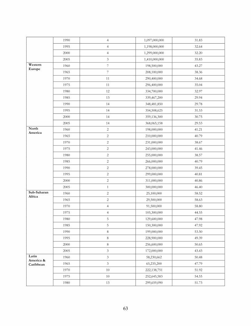
63

1990 4 1,097,000,000 31.83

1995 4 1,198,000,000 32.64

2000 4 1,299,000,000 32.20

2005 3 1,410,000,000 35.83 Western Europe

1960 7 198,500,000 43.27

1965 7 208,100,000 38.36

1970 11 290,400,000 34.68

1975 11 296,400,000 35.04

1980 12 334,700,000 32.97

1985 13 339,467,200 29.94

1990 14 348,481,850 29.78

1995 14 354,508,625 31.53

2000 14 359,136,300 30.75

2005 14 368,065,158 29.53 North America

1960 2 198,000,000 41.21

1965 2 210,000,000 40.79

1970 2 231,000,000 38.67

1975 2 243,000,000 41.46

1980 2 255,000,000 38.57

1985 2 266,000,000 40.79

1990 2 278,000,000 39.45

1995 2 299,000,000 40.81

2000 2 311,000,000 40.86

2005 1 300,000,000 46.40 Sub-Saharan Africa

1960 2 25,100,000 58.52

1965 2 29,500,000 58.63

1970 4 91,500,000 58.80

1975 4 105,300,000 44.55

1980 5 129,600,000 47.98

1985 5 150,300,000 47.92

1990 8 199,000,000 53.50

1995 8 228,900,000 49.39

2000 8 256,600,000 50.65

2005 3 172,000,000 43.43

Latin America & Caribbean

1960 3 58,230,662 50.48

1965 3 65,235,200 47.79

1970 10 222,138,751 51.92

1975 10 252,645,583 54.55

1980 13 299,659,090 51.73

64

1985 14 349,033,393 50.39

1990 18 405,355,167 52.94

1995 18 438,780,381 54.17

2000 18 471,603,150 54.82

2005 18 509,623,295 53.14

65

Table 2A: Average Trade to GDP ratio (Trade openness) for each region

Region Periods Number of Countries Trade to GDP ratio (%)

East Asia Pacific

1960 3 41.94

1965 5 32.65

1970 7 39.07

1975 7 49.06

1980 8 73.93

1985 9 69.95

1990 9 83.14

1995 10 95.68

2000 10 112.53

2005 9 142.91

Europe & Central Eurasia

1960 1 43.54

1965 1 58.79

1970 1 62.58

1975 2 52.74

1980 3 54.61

1985 3 67.72

1990 16 77.45

1995 21 89.49

2000 21 104.10

2005 18 105.64

Middle East & North

Africa

1960 5 33.41

1965 6 39.08

1970 5 47.52

1975 5 61.07

1980 5 68.62

1985 5 68.94

1990 6 66.93

1995 6 63.02

2000 6 66.97

2005 3 61.20

South Asia

1960 2 15.54

1965 2 15.83

1970 4 26.27

1975 4 29.78

1980 4 40.64

1985 4 32.26

66

1990 4 35.62

1995 4 42.28

2000 4 44.34

2005 3 39.14

Western Europe

1960 6 53.51

1965 6 49.13

1970 11 56.44

1975 11 61.15

1980 12 65.18

1985 13 81.73

1990 14 77.65

1995 14 83.35

2000 14 105.35

2005 14 105.27

North America

1960 2 22.34

1965 2 23.41

1970 2 26.68

1975 2 31.36

1980 2 37.53

1985 2 35.71

1990 2 36.02

1995 2 47.41

2000 2 55.87

2005 1 26.93

Sub-Saharan Africa

1960 2 60.36

1965 2 58.08

1970 4 47.66

1975 4 59.59

1980 5 63.31

1985 5 54.25

1990 8 61.03

1995 8 69.31

2000 8 78.69

2005 7 82.27

Latin America & Caribbean

1960 4 46.59

1965 4 47.51

1970 10 45.26

1975 10 49.88

1980 13 58.02

67

1985 15 57.61

1990 19 59.83

1995 19 64.73

2000 18 65.88

2005 17 71.78

68

Table 2B: Weighted Average Trade to GDP ratio (Trade openness) for each region

Region Periods Number of Countries Total Population Weighted Average Trade to GDP ratio (%)

East Asia Pacific

1960 3 43,100,000 30.75

1965 5 248,500,000 19.38

1970 7 315,800,000 29.34

1975 7 346,100,000 41.02

1980 8 392,200,000 51.00

1985 9 469,800,000 44.92

1990 9 506,100,000 52.55

1995 10 544,900,000 61.63

2000 10 592,600,000 79.10

2005 9 487,400,000 96.05 Europe & Central Eurasia

1960 1 10,000,000 43.54

1965 1 10,000,000 58.79

1970 1 10,000,000 62.58

1975 2 52,000,000 31.34

1980 3 65,900,000 34.31

1985 3 70,900,000 48.62

1990 16 248,300,000 55.73

1995 21 285,300,000 71.45

2000 21 285,900,000 83.26

2005 18 210,500,000 93.68 Middle East & North Africa

1960 5 59,300,000 37.36

1965 6 69,900,000 38.15

1970 5 40,900,000 41.92

1975 5 44,200,000 55.02

1980 5 48,700,000 58.68

1985 5 53,400,000 62.92

1990 6 114,800,000 58.92

1995 6 125,500,000 56.84

2000 6 134,900,000 53.46

2005 3 99,000,000 62.37

South Asia 1960 2 484,000,000 12.61

1965 2 551,000,000 10.22

1970 4 692,000,000 11.16

1975 4 774,000,000 15.10

1980 4 878,000,000 19.57

1985 4 981,000,000 16.42

69

1990 4 1,097,000,000 19.26

1995 4 1,198,000,000 25.86

2000 4 1,299,000,000 28.99

2005 3 1,410,000,000 41.40 Western Europe

1960 6 125,500,000 42.35

1965 6 132,100,000 39.05

1970 11 290,400,000 41.90

1975 11 296,400,000 47.95

1980 12 334,700,000 51.16

1985 13 339,467,200 56.69

1990 14 348,481,850 52.53

1995 14 354,508,625 56.51

2000 14 359,136,300 69.57

2005 14 368,065,158 70.34 North America

1960 2 198,000,000 11.89

1965 2 210,000,000 12.25

1970 2 231,000,000 14.07

1975 2 243,000,000 18.99

1980 2 255,000,000 24.04

1985 2 266,000,000 20.80

1990 2 278,000,000 23.66

1995 2 299,000,000 28.03

2000 2 311,000,000 32.23

2005 1 300,000,000 26.93 Sub-Saharan Africa

1960 2 25,100,000 58.80

1965 2 29,500,000 56.65

1970 4 91,500,000 33.30

1975 4 105,300,000 49.91

1980 5 129,600,000 56.22

1985 5 150,300,000 41.98

1990 8 199,000,000 61.03

1995 8 228,900,000 73.32

2000 8 256,600,000 76.29

2005 7 256,000,000 75.11

Latin America & Caribbean

1960 4 68,130,662 22.04

1965 4 76,235,200 18.21

1970 10 222,138,751 19.59

1975 10 252,645,583 23.55

1980 13 299,659,090 26.91

70

1985 15 349,287,837 27.68

1990 19 405,614,835 32.53

1995 19 439,038,371 37.48

2000 18 469,254,806 41.89

2005 17 506,853,251 45.88

71

APPENDIX V

Average important variables for each country in the study during 1960-2005 period:

Country Gini (%) GDP per capita ($) Trade/GDP (%) Export/GDP (%) Import/GDP (%) Life Expectancy (year)

Albania 29.5 3,324.62 57.404 17.9613 39.4426 74.4563

Argentina 43.2467 11,071.50 17.8656 9.80153 8.06408 70.6741

Armenia 39.25 5,119.60 78.3519 27.7788 50.5731 70.2868

Australia 29.85 21,636.10 33.7601 16.1427 17.6173 75.0174

Austria 28.4063 24,365.90 74.7361 37.7584 36.9777 74.6017

Azerbaijan 42.8875 4,122.04 86.4401 43.4349 43.0053 66.3695

Bahamas 47.375 22,695.30 116.496 57.2132 59.2831 69.5848

Bangladesh 36.7968 1,618.58 23.7006 8.946 14.7546 52.8647

Barbados 36.1 17,702.10 119.957 56.5728 63.3841 72.4602

Belgium 30.9617 23,150.60 132.78 67.2403 65.5393 75.1583

Bolivia 53.6933 3,180.19 50.1042 23.6402 26.4639 60.8118

Brazil 57.9059 7,612.71 19.0984 9.55402 9.54437 66.1544

Bulgaria 25.7017 5,578.74 94.4328 45.3802 49.0526 71.2153

Cambodia 44.0667 1,901.28 108.736 48.3717 60.3643 56.96

Canada 31.8944 21,199.00 53.1011 27.2593 25.8418 75.0166

Chile 52.9432 9,983.05 55.1935 28.4037 26.7898 72.4869

Colombia 53.598 5,722.14 32.946 16.2365 16.7096 67.9628

Costa Rica 45.6254 8,191.73 74.0302 34.5972 39.4331 74.769

Cote d' Ivoire 44.8722 2,655.41 76.4578 41.1176 35.3403 56.4963

Croatia 28.4 10,265.30 84.4611 39.2245 45.2366 72.9982

Denmark 32.1817 21,269.80 71.4026 36.1083 35.2943 74.5111

Dominican Rep. 48.45 5,241.35 64.2461 28.6168 35.6293 66.7565

Ecuador 51.1375 5,179.25 62.4224 31.6619 30.7605 72.1338

Egypt 34.4802 3,469.81 47.2455 21.033 26.2125 62.6321

El Salvador 48.26 4,881.67 62.6823 23.5292 39.1531 68.8304

Estonia 32.8232 10,880.40 161.63 77.8901 83.74 70.1913

Finland 29.7549 18,564.70 57.2049 29.0326 28.1722 73.4855

France 36.051 19,686.00 40.9783 20.5031 20.4752 74.9188

Georgia 38.15 4,620.85 75.3611 30.5478 44.8133 70.3721

Germany 32.5558 28,943.50 51.3315 25.397 25.9345 73.6825

Ghana 39.9111 1,357.47 76.5174 30.6474 45.8702 57.6669

Greece 37.44 15,584.00 43.0103 16.6296 26.3807 74.5163

Honduras 55.098 3,172.81 96.1545 43.7956 52.359 66.8553

72

Hong Kong 44.1 24,666.00 241.749 122.707 119.042 77.6098

Hungary 23.475 11,041.80 84.8112 41.6224 43.1889 69.6565

India 34.1637 1,789.74 17.7931 8.01733 9.77577 55.1071

Indonesia 34.26 2,788.15 46.6544 25.1169 21.5374 57.8911

Ireland 34.75 26,980.60 145.891 78.246 67.6454 76.5616

Israel 37.1889 14,737.70 75.4527 31.0708 44.3819 74.3547

Italy 35.44 21,156.60 43.8224 22.0433 21.779 76.0465

Jamaica 50.7427 7,483.38 97.7383 45.668 52.0702 71.0061

Japan 34.3815 18,422.30 21.9786 11.5129 10.4657 75.3408

Kazakhstan 33.36667 9,187.35 95.4969 49.7063 45.7906 66.6407

Kenya 59.6556 1,878.37 61.6246 28.5367 33.088 54.8921

Korea, Rep. of 35.1579 9,291.07 54.0937 25.0622 29.0315 66.9935

Latvia 31.4208 8,778.44 96.1698 44.9684 51.2013 69.3466

Lithuania 28.59 7,732.00 105.948 48.6721 57.276 70.6251

Luxembourg 27.788 51,833.60 231.637 125.11 106.517 76.538

Malawi 51.9437 943.43 64.5531 25.2176 39.3355 46.0343

Malaysia 48.9492 7,590.98 131.847 69.3537 62.4934 67.4829

Mali 45.6556 1,041.48 59.3303 22.6663 36.6639 50.2621

Mauritania 46.3833 2,030.19 110.114 41.2164 68.8978 60.487

Mexico 51.915 7,944.92 33.668 16.3963 17.2717 67.0394

Moldova 32.5333 2,770.70 118.528 49.6232 68.9049 66.6587

Morocco 47.2556 3,527.32 51.1426 22.9373 28.2053 58.044

Netherlands 31.0267 22,057.40 108.009 55.5714 52.4376 75.869

New Zealand 41.75 17,332.00 57.7074 27.9807 29.7266 74.3215

Nicaragua 52.1912 2,041.13 71.977 24.256 47.721 68.4725

Nigeria 48.2042 1,505.53 57.5252 32.5566 24.9686 46.0343

Norway 30.4721 30,280.40 75.4688 41.0518 34.417 76.6767

Pakistan 32.8031 1,990.26 32.9918 12.864 20.1278 56.1962

Paraguay 52.2133 4,756.59 99.354 45.5243 53.8297 69.6875

Peru 47.4418 4,751.11 37.1623 18.9598 18.2025 64.1178

Philippines 46.175 3,578.37 79.0897 38.1722 40.9176 67.5002

Poland 27.695 8,446.08 57.3908 29.0121 28.3787 70.9712

Portugal 36.1875 11,796.90 56.3652 24.6505 31.7147 71.3577

Romania 31.6042 6,867.91 62.827 27.5336 35.2934 70.4939

Singapore 44.8937 19,369.30 444.315 236.445 207.87 72.9452

Slovak Rep. 23.9333 12,167.10 119.01 57.7675 61.2421 72.5728

Slovenia 25.9458 18,056.80 126.814 64.205 62.6096 75.0529

South Africa 53.6722 7,594.08 52.8017 27.5695 25.2322 55.5158

Spain 31.7515 20,538.40 45.0969 21.5495 23.5474 77.6606

73

Sri Lanka 37.8718 2,911.89 72.2876 30.8526 41.435 68.5032

Sweden 33.1908 20,783.10 63.7324 32.8729 30.8595 76.8352

Taiwan 31.4352 8,593.63 - - - -

Tajikistan 31.91 2,064.57 119.76 54.5423 65.2176 63.4652

Thailand 45.2677 4,934.57 78.2856 37.5816 40.704 66.9884

Tunisia 43.85 4,742.92 72.6036 34.6791 37.9245 61.5845

Turkey 44.6356 5,030.89 30.9917 13.1343 17.8575 65.1008

Turkmenistan 28.9 7,923.17 172.31 89.7373 82.5727 62.3833

Ukraine 34.8825 6,643.00 93.8926 47.1599 46.7327 68.2685

United Kingdom 31.1333 19,069.10 50.5728 24.8599 25.7128 74.5161

United States 41.7083 27,161.20 18.1679 8.45766 9.71021 73.7227

Uruguay 43.2 9,699.02 43.1398 21.9034 21.2363 73.0966

Uzbekistan 30.4167 1,645.11 61.3152 29.8061 31.5091 67.4311

Venezuela 46.2656 11,287.00 49.7387 29.8256 19.9131 70.0205

Average important variables for each region in the study during 1960-2005 period:

Region Gini (%) GDP per capita ($)

Trade/GDP (%)

Export/GDP (%)

Import/GDP (%)

Life Expectancy (year)

East Asia Pacific 39.1424 12,241.90 81.0858 40.6437 40.442 69.6956

Europe & Central Eurasia 30.9564 7,546.50 90.1557 42.2146 47.9411 69.1342

Middle East & North Africa 39.9311 9,556.86 57.6426 25.0482 32.5944 67.649

South Asia 35.5008 2,009.97 33.8539 13.9575 19.8963 57.585

Western Europe 31.8772 23,717.20 77.8816 40.0456 37.8361 75.299

North America 37.0597 24,337.00 34.7152 17.3637 17.3515 74.3356

Sub-Saharan Africa 50.7391 2,756.35 66.0728 30.5574 35.5154 52.9903

Latin American & Caribbean 49.309 8,658.57 59.8373 28.5722 31.2651 69.1831

74

REFERENCES

1. Milanovic B. 2006. Global Income Inequality: What It Is And Why It Matters. DESA Working

Paper No. 26.

2. Aradhyula, S., Rahman, T,. and Seenivasan, K. 2007. Impact of International Trade on Income and

Income Inequality. Selected paper for presentation at the American Agricultural Economics

Association Annual meeting in Portland, OR.

3. Santos-Paulino, A.U. 2012. Trade, Income Distribution and Poverty in Developing Countries: A

Survey. United Nations Conference on Trade and Development (UNCTAD).

4. Kahai, Simran K. and Walter Simmons. 2005. The Impact of Globalization on Income Inequality.

Global Business and Economics Review 7.1 (2005): 1-15.

5. Dollar, D., and Kraay, A. 2001. Growth Is Good For the Poor. World Bank Policy Research

Working Paper No. 2587.

6. Anderson, E. 2005. Openness and Inequality in Developing Countries: A Review of Theory and

Recent Evidence. World Development. Vol.33, No.7.

7. Calderon, C., and Chong, A. 2001. External Sector and Income Inequality in Independent

Economies using Dynamic panel data approach. Economic Letters. 71.

8. Ghose, Ajit K. 2001. Global Inequality and International Trade. Camb. J. Econ. 28.

9. Cornia, Giovanni Andrea. 2003. The Impact of Liberalization and Globalization on Income

Inequality in Developing and Transitional Economies. CESifo Working Paper Series No. 843.

10. Spilimbergo, Antonio & Londono, Juan Luis & Szekely, Miguel. 1999. Income Distribution,

Factor Endowments, and Trade Openness. Journal of Development Economics. Elsevier. Vol.59.

11. Baltagi, Badi H. 2005. Econometric Analysis of Panel Data. John Wiley & Sons Limited. West

Sussex PO198SQ, England.

75

12. Goldberg PK and Pavcnik N. 2007b. Distributional Effects of Globalization in Developing

countries. Journal of Economic Literature. 45(1): 39-82.

13. http://www.oecd-library.org

14. https://en.wikipedia.org/wiki/Gini_coefficient

15.http://www.elgarblog.com/2012/07/31/trade-facilitation-defining-measuring-explaining-and-

reducing-the-cost-of-international-trade/

16. http://data.worldbank.org/indicator#topic-21

17. https://www.cia.gov/library/publications/the-world-factbook/rankorder/2172rank.html

18. http://inequality.org/unequal-americas-income-distribution/

19. Pablo García Silva. 1999. Income Inequality and the Real Exchange Rate. Central Bank of Chile

Working paper. No.54.

20. Wooldridge, J.M. 2013. Introductory Econometrics: A modern approach. 5th Edition. South-

Western Cengage Learning.

21. Feenstra, R. C., Taylor, A. M. 2014.“International Trade” 3rd Edition. Worth Macmillan.