Trade openness and economicgrowth: further evidence without

relying on data stationarityH. Aydin Okuyan

Department of Administrative Sciences and Economics,Balikesir University, Balikesir, Turkey

Alper OzunSchool of Management, Bradford University, Bradford, UK, and

Erman ErbaykalDepartment of Economics, Istanbul University, Istanbul, Turkey

Abstract

Purpose – The purpose of this paper is to investigate the relationship between trade openness andeconomic growth in developing countries. Under this aim, the co-integration relationship betweentrade openness and economic growth of 17 developing countries is examined without relying on datastationarity.

Design/methodology/approach – The co-integration relationship between trade openness andeconomic growth is analyzed by Bounds testing approach developed by Pesaran et al. In addition tothis, the causality relationship is tested by causality analysis developed by Toda and Yamamoto.

Findings – According to the Bounds test results, co-integration relationship has been detected for sixcountries and long-term coefficients among the variables have been found positive and statisticallysignificant. According to the Toda and Yamamoto causality analysis, causality has been detected foreight countries. In four of these, the direction of causality is from trade openness to economic growthand in the other four, vice versa.

Originality/value – The methodology employed provides an alternative framework for examiningrelationship among economic variables. The paper shows how to create co-integration and causalitytests without relying on data stationarity, which is a major problem in time series of economicvariables. On the empirical side, it adds new empirical results into the literature in the name ofidentification of relationship between trade openness and economic growth in developing countries.

KeywordsDeveloping countries, Economic growth, International trade, Econometrics, Data stationarity

Paper type Research paper

Motivation and a literature reviewThere is a commonly accepted opinion in the economic literature that the openeconomies grow faster compared to the closed economies. The globalization movementwhich accelerated especially in the 1980s enabled this condition to come into view moreclearly. In this period, the globalization movement materialized in two stages, namelyfinancial and trade openness, and trade openness was accepted as the prerequisite forfinancial openness. Trade openness defines the approach which aims to removegovernmental controls on the trade of goods and services and to provide internationalfree trade. Financial openness is the sum of the policies which primarily aim to remove

The current issue and full text archive of this journal is available at

www.emeraldinsight.com/1056-9219.htm

JEL classification – O11, F43, F14, C82

IJCOMA22,1

26

International Journal of Commerceand ManagementVol. 22 No. 1, 2012pp. 26-35q Emerald Group Publishing Limited1056-9219DOI 10.1108/10569211211204492

interventions and controls of the government on domestic banking and other financialinstruments and second, to envisage the integration of the domestic financial marketsinto international markets (Dagdelen, 2004). Consequently, openness term can bedefined as the removal of restrictions which prevent the international circulation of thegoods, services, labor, and capital. According to the basic neoclassical growth model(Solow, 1956), there is no relationship between openness and economic growth. Beingthe primary determinant of long-term economic growth, this model observes thechange in the technology and population growth rate and asserts that growth will notarise from the relations between the countries. Endogenous growth theories(Romer, 1990) argue that trade openness can increase growth by means ofexpansion effect or technology transfer.

Accordingly, in an economy which is open to international trade, especially exportoriented sectors must maintain technological development in order to compete with thequality and prices of foreign goods and services. Furthermore, technology can also bedeveloped by means of foreign goods. In doing so, underdeveloped countries whoseR&D facilities are limited find the opportunity to gain technology faster via copying.When the empirical literature is examined, it is observed that there are studies whichset forth a number of effects of trade openness on the economy. According to Esfahani(1991), the foreign exchange which is obtained by trade openness assists the country todecrease the foreign exchange restriction and assists intermediate goods, such as rawmaterial which cannot be produced domestically, and capital goods to increase. In thisway, decreases can be maintained in savings – investment and import – export deficit.Moreover, trade openness creates a factor competition by facilitating the production ofnew technologies which are suitable for the demand oriented to the goods of theexporter country and accordingly expands the production opportunities (Alam, 1991).Trade openness provides distribution of information between countries and leads toincrease in production efficiency (Miller and Upadhyay, 2000). In addition to theseviews, Grossman and Helpman (1991) stated that developing countries can increasetheir growth by copying innovative inventions made by developed countries thanks totrade openness. Rodrigez and Rodrik (2000) argued that trade restrictions negativelyaffect growth, but they state that no adequate finding was found on the fact that tradeopenness positively affects the growth. On the other hand, they came to a conclusionthat openness is useful in terms of transferring technology. There are many studies inthe literature which conclude that openness positively affects economic growth (Dollar,1992; Frankel et al., 1996; Edwards, 1993, 1997, 1998; Levine, 1997; Ben-David andLoewy, 1998; Gwartney et al., 2000; Rutherford and Tarr, 2002; Yanıkkaya, 2003; Dollarand Kraay, 2004; Utkulu and Ozdemir, 2004; Badinger, 2005).

In the literature, there are studies which argue that trade openness negativelyaffects economic growth and/or tries to set forth the negative effects of trade opennesson growth. Odekon (2002) and Galindo et al. (2002) assert that trade and financialopenness decreases growth and they listed the reasons for this condition. According tothese studies, factors which arise as a result of the increase in trade openness as well asthe increase in transaction costs due to the increase in the lending costs, the emergenceof the distribution of the loans to the ineffective areas, succeeding in preventing thecapital from gravitating towards effective and profitable sectors in a country whichhas a comparative superiority, and information asymmetry, have negative effects ongrowth. In view of the studies within the literature, it can be stated that no certain

Trade opennessand economic

growth

27

agreement has been achieved on the effect of trade openness on economic growth. Sofar, the studies which examine the relationship between trade openness and growthhave been criticized owing to reasons such as method and data quality. In this study,data coming from many developing countries will be examined with the same methodand there will be an opportunity to compare them with each other. For that reason, thecontribution which will be made to the literature by the study holds importancein terms of presenting the differences between the countries. The aim of this study is toset forth the relationships between trade openness and economic growthin 17 developing countries. The study is composed of four sections. In the firstsection, the subject has been introduced and the results of the previous studiesconducted on this subject have been mentioned. In the second section, the data set andmethodology have been presented. In the third section, empirical evidence has beengiven. The fourth section is composed of results and assessments.

Data and methodologyThe relationship between trade openness and economic growth is investigated byexamining the data of 17 developing countries. These countries were chosen from thedeveloping countries included in the 2005 report from the Institute of InternationalFinance. On total, 29 developing countries of the report were classified in four groups:Asia/Pacific, Latin America, Europe, and Africa/Middle East. About 17 countries ofwhich the data suitable for time series analysis could be reached were chosen amongthese 29 countries in this study. These countries are China, India, Indonesia, Malaysia,Philippines, Singapore, South Korea, and Thailand in the Asia/Pacific group; Brazil,Chile, Argentina, Peru, and Mexico from Latin America; Morocco, Egypt, Republic ofSouth Africa, and Algeria from the Africa/Middle East group. Logarithmic value ofsum of “import þ export” in US dollars was taken as the representative of tradeopenness. Logarithmic value of reel GDP in US dollars was taken as the representativeof economic growth. Two variables denoted as LY and LOP. All data were obtainedfrom the IMF statistics data base. The data covers the period: 1960-2003 for Algeria,1952-2004 for China, 1950-2003 for India, 1960-2004 for Indonesia, 1955-2003 forMalaysia, 1950-2004 for the Philippines, 1960-2004 for Singapore, 1953-2004 for SouthKorea, 1950-2003 for Thailand, 1950-2003 for Brazil, 1951-2004 for Chile, 1950- 2004 forArgentina, 1950-2003 for Peru, 1950-2004 for Mexico, 1950-2003 for Morocco,1950-2003 for Egypt, and 1950-2004 for Republic of South Africa.

Empirical studies show that, most of the time, a series is not stationary. Since facinga spurious regression problem among these series which include a unit root, somemethods are suggested to solve this problem. One of them is taking the differences ofthe series and then putting them into regressions. However, in this case, we areconfronted with a new problem. This method leads to the loss of information that isimportant for the long-run equilibrium. As long as the first differences of the variablesare used, determining a potential long-run relationship between these variablesbecomes impossible. This is the point of origin of co-integration analysis.

The co-integration approach developed by Engel and Granger (1987) overcame thisproblem. According to this approach, time series which are not stationary at levels butstationary in the first difference can be modeled with their level states. In this way, loss ofinformation in the long run can be prevented. However, this approach becomes invalid ifthere are more than one co-integration vectors. Moving from this point, with the help

IJCOMA22,1

28

of the approach developed by Johansen (1988), it is possible to test how manyco-integration vectors there are among the variables by using the VAR model in whichall the variables are accepted as endogenous. Therefore, unlike the Engle-Grangermethod, a more realistic examination is provided without limiting the test in oneco-integration vector expectation. However, in order to perform these tests developed byEngel and Granger (1987), Johansen (1988), and Johansen and Juselius (1990), theconditions must be met that all series should not be stationary at the levels and theyshould become stationary when the same differences are taken. If one or more of theseries are stationary at levels, that is to say I(0), the co-integration relationship cannot beexamined with these tests. Bounds test approach developed by Pesaran et al. (2001)eliminates this problem. This approach has two main advantages. First, it can be appliedirrespective of whether the regressors are I(0), I(1), or even integrated of the same order.Second, Bounds test procedure is robust for co-integration analysis with small samplestudy.

When we examine the methodology used in causality aspect, we see that causalitytest developed by Granger (1969) is performed if the series are stationary in their levelconditions. Vector error correction (VEC) model developed by Engel and Granger(1987) is used widely if co-integration occurs between series which become stationarywhen the same difference is taken. In the VEC model which is a limited VAR model,F-test is used for testing the causality. However; if the series are cointegrated,traditional F-test statistics used for testing the Granger causality may not be validbecause it does not fit into the standard distribution (Toda and Yamamoto, 1995; Gilesand Mirza, 1998; Giles and Williams, 1999). In the causality testing performed with themodified WALD method developed by Toda and Yamamoto (1995), co-integrationrelationship between the series is not important and it is enough to determine the rightmodel and to know the maximum co-integration level of the variables in the model.Bounds test developed by Pesaran et al. (2001) has been applied to examine theco-integration relationship between the variables in this study. To investigate thecausality relationship between the variables, Toda and Yamamoto (1995) causalityanalysis is used which does not require a co-integration condition between the series.

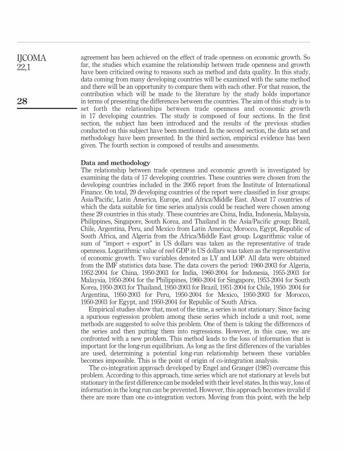
Empirical evidenceStationary testBefore testing for co-integration and causality, we tested for unit roots to find thestationarity properties of the data. Augmented Dickey-Fuller (ADF) t-tests (Dickey andFuller, 1981) and Phillips and Perron (1988), tests were used on each of the two timeseries for Turkey. Akaike information criterion is used to determine the duration ofdelays in both tests. The results of these tests are given in Table I.

Checking the results in Table I, the pre-condition for examination of long-termrelationship between variables by Pesaran Bounds test that the independent variablesare I(0) or I(1) is satisfied according to both ADF and PP unit root tests. Besides, as themaximum co-integration degree is found I(1) for each country, 1 will be added to the lagnumber of each country when Toda-Yamamoto causality test is applied.

The Bounds test approach to co-integrationFirst, an unrestricted error correction model (UECM) is formed. The form of this modeladapted into our study is as follows:

Trade opennessand economic

growth

29

ADF test PP testCountries Variables Without trend With trend Without trend With trend

Algeria LY 22.928 22.157 0.980 23.539 * *

DLY 26.192 * 22.757 26.196 * 27.248 *

LOP 21.095 21.314 0.875 21.414DLOP 26.568 * 26.533 * 26.568 * 26.533 *

Argentina LY 21.947 22.434 21.500 22.190DLY 26.154 * 26.232 * 26.398 * 26.338 *

LOP 20.203 23.213 20.103 22.555DLOP 26.078 * 26.138 * 26.078 * 26.138 *

Brazil LY 22.709 20.047 22.678 20.271DLY 24.914 * 25.846 * 25.025 * 25.839 *

LOP 0.146 22.649 20.334 21.785DLOP 25.540 * 25.546 * 25.701 * 25.698 *

Chile LY 0.003 21.338 0.338 21.317DLY 25.366 * 25.381 * 25.394 * 25.408 *

LOP 20.296 23.386 20.220 23.116DLOP 26.247 * 26.169 * 26.250 * 26.153 *

China LY 0.730 20.944 3.398 20.818DLY 20.999 25.479 * 24.591 * 25.605 *

LOP 1.003 21.518 1.378 21.265DLOP 24.908 * 25.131 * 23.626 * 3.800 * *

Egypt LY 0.974 22.840 0.893 22.624DLY 26.278 * 26.478 * 27.757 * 28.284 *

LOP 20.633 22.118 20.684 21.819DLOP 25.821 * 25.763 * 25.838 * 25.780 *

India LY 1.839 21.100 3.930 20.740DLY 26.639 * 26.904 * 26.632 * 27.462 *

LOP 0.158 22.944 0.225 22.274DLOP 26.565 * 26.639 * 26.564 * 26.637 *

Indonesia LY 20.533 23.476 20.389 22.336DLY 23.747 * 23.853 * * 24.851 * 24.777 *

LOP 20.832 21.763 20.851 21.492DLOP 23.952 23.921 * * 23.902 * 23.861 *

South Korea LY 1.173 22.682 0.923 22.892DLY 25.677 * 25.735 * 25.712 * 25.738 *

LOP 21.733 22.740 20.377 21.389DLOP 26.299 * 24.435 * 26.305 * 26.314 *

Malaysia LY 0.306 22.535 0.211 22.783DLY 25.739 * 25.687 * 25.713 * 25.663 *

LOP 20.032 23.255 0.111 22.340DLOP 25.019 * 24.966 * 25.038 * 24.990 *

Mexico LY 22.139 21.590 22.041 21.301DLY 25.252 * 25.490 * 25.252 * 25.436 *

LOP 20.322 22.490 20.021 22.196DLOP 24.017 * 23.968 * * 24.051 * 24.003 * *

Morocco LY 21.396 20.963 21.048 21.309DLY 27.881 * 25.206 * 27.842 * 27.932 *

LOP 0.108 22.541 20.160 21.923DLOP 26.002 * 25.982 * 26.003 * 25.961 *

Peru LY 21.848 21.712 22.384 21.815

(continued )Table I.Stationary test results

IJCOMA22,1

30

DLYt ¼ a0 þXm

i¼1

a1iDLYt2i þXm

i¼0

a2iDLOPt2i þ a3LYt21 þ a4LOPt21 þ mt ð1Þ

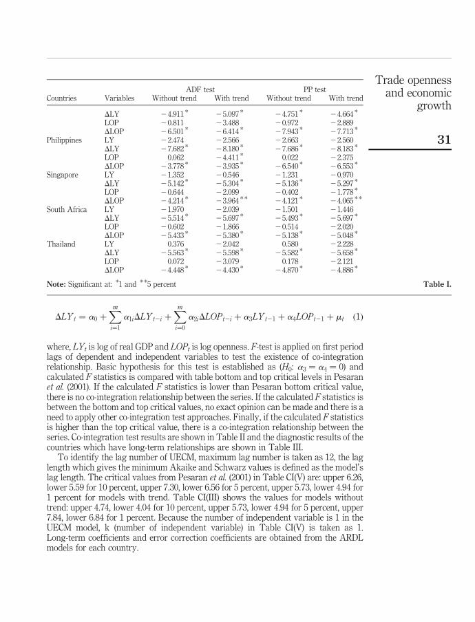
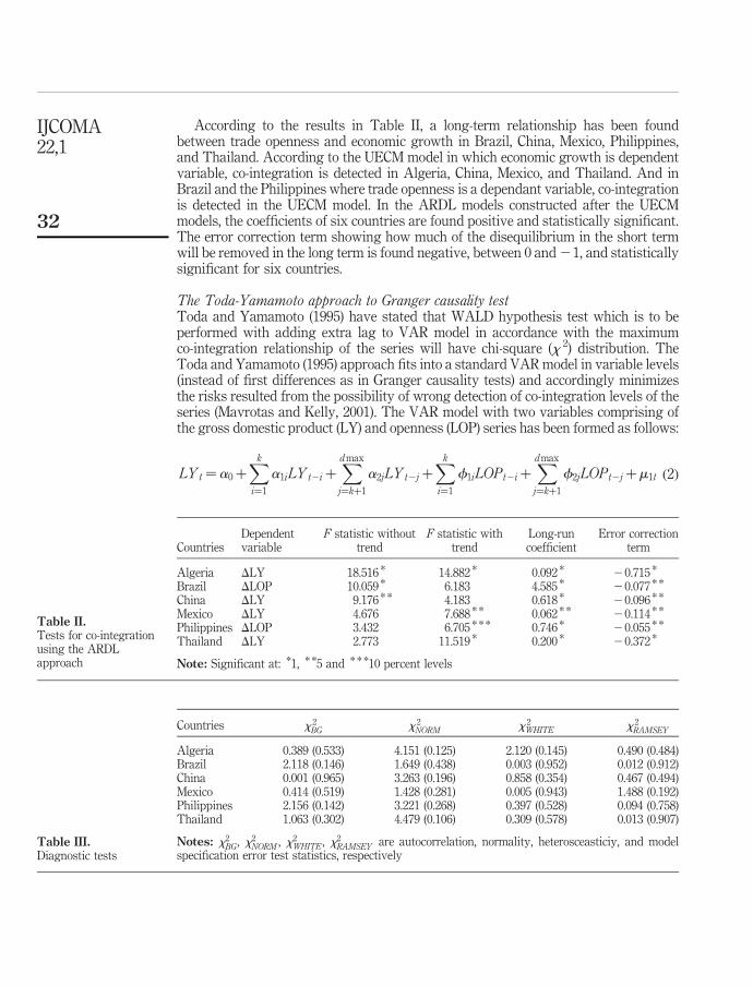
where, LYt is log of real GDP and LOPt is log openness. F-test is applied on first periodlags of dependent and independent variables to test the existence of co-integrationrelationship. Basic hypothesis for this test is established as (H0: a3 ¼ a4 ¼ 0) andcalculated F statistics is compared with table bottom and top critical levels in Pesaranet al. (2001). If the calculated F statistics is lower than Pesaran bottom critical value,there is no co-integration relationship between the series. If the calculated F statistics isbetween the bottom and top critical values, no exact opinion can be made and there is aneed to apply other co-integration test approaches. Finally, if the calculated F statisticsis higher than the top critical value, there is a co-integration relationship between theseries. Co-integration test results are shown in Table II and the diagnostic results of thecountries which have long-term relationships are shown in Table III.

To identify the lag number of UECM, maximum lag number is taken as 12, the laglength which gives the minimum Akaike and Schwarz values is defined as the model’slag length. The critical values from Pesaran et al. (2001) in Table CI(V) are: upper 6.26,lower 5.59 for 10 percent, upper 7.30, lower 6.56 for 5 percent, upper 5.73, lower 4.94 for1 percent for models with trend. Table CI(III) shows the values for models withouttrend: upper 4.74, lower 4.04 for 10 percent, upper 5.73, lower 4.94 for 5 percent, upper7.84, lower 6.84 for 1 percent. Because the number of independent variable is 1 in theUECM model, k (number of independent variable) in Table CI(V) is taken as 1.Long-term coefficients and error correction coefficients are obtained from the ARDLmodels for each country.

ADF test PP testCountries Variables Without trend With trend Without trend With trend

DLY 24.911 * 25.097 * 24.751 * 24.664 *

LOP 20.811 23.488 20.972 22.889DLOP 26.501 * 26.414 * 27.943 * 27.713 *

Philippines LY 22.474 22.566 22.663 22.560DLY 27.682 * 28.180 * 27.686 * 28.183 *

LOP 0.062 24.411 * 0.022 22.375DLOP 23.778 * 23.935 * 26.540 * 26.553 *

Singapore LY 21.352 20.546 21.231 20.970DLY 25.142 * 25.304 * 25.136 * 25.297 *

LOP 20.644 22.099 20.402 21.778 *

DLOP 24.214 * 23.964 * * 24.121 * 24.065 * *

South Africa LY 21.970 22.039 21.501 21.446DLY 25.514 * 25.697 * 25.493 * 25.697 *

LOP 20.602 21.866 20.514 22.020DLOP 25.433 * 25.380 * 25.138 * 25.048 *

Thailand LY 0.376 22.042 0.580 22.228DLY 25.563 * 25.598 * 25.582 * 25.658 *

LOP 0.072 23.079 0.178 22.121DLOP 24.448 * 24.430 * 24.870 * 24.886 *

Note: Significant at: *1 and * *5 percent Table I.

Trade opennessand economic

growth

31

According to the results in Table II, a long-term relationship has been foundbetween trade openness and economic growth in Brazil, China, Mexico, Philippines,and Thailand. According to the UECM model in which economic growth is dependentvariable, co-integration is detected in Algeria, China, Mexico, and Thailand. And inBrazil and the Philippines where trade openness is a dependant variable, co-integrationis detected in the UECM model. In the ARDL models constructed after the UECMmodels, the coefficients of six countries are found positive and statistically significant.The error correction term showing how much of the disequilibrium in the short termwill be removed in the long term is found negative, between 0 and 21, and statisticallysignificant for six countries.

The Toda-Yamamoto approach to Granger causality testToda and Yamamoto (1995) have stated that WALD hypothesis test which is to beperformed with adding extra lag to VAR model in accordance with the maximumco-integration relationship of the series will have chi-square (x 2) distribution. TheToda and Yamamoto (1995) approach fits into a standard VAR model in variable levels(instead of first differences as in Granger causality tests) and accordingly minimizesthe risks resulted from the possibility of wrong detection of co-integration levels of theseries (Mavrotas and Kelly, 2001). The VAR model with two variables comprising ofthe gross domestic product (LY) and openness (LOP) series has been formed as follows:

LYt ¼a0 þXk

i¼1

a1iLY t2iþXdmax

j¼kþ1

a2jLY t2jþXk

i¼1

f1iLOPt2iþXdmax

j¼kþ1

f2jLOPt2jþm1t ð2Þ

CountriesDependentvariable

F statistic withouttrend

F statistic withtrend

Long-runcoefficient

Error correctionterm

Algeria DLY 18.516 * 14.882 * 0.092 * 20.715 *

Brazil DLOP 10.059 * 6.183 4.585 * 20.077 * *

China DLY 9.176 * * 4.183 0.618 * 20.096 * *

Mexico DLY 4.676 7.688 * * 0.062 * * 20.114 * *

Philippines DLOP 3.432 6.705 * * * 0.746 * 20.055 * *

Thailand DLY 2.773 11.519 * 0.200 * 20.372 *

Note: Significant at: *1, * *5 and * * *10 percent levels

Table II.Tests for co-integrationusing the ARDLapproach

Countries x 2BG x 2

NORM x 2WHITE x 2

RAMSEY

Algeria 0.389 (0.533) 4.151 (0.125) 2.120 (0.145) 0.490 (0.484)Brazil 2.118 (0.146) 1.649 (0.438) 0.003 (0.952) 0.012 (0.912)China 0.001 (0.965) 3.263 (0.196) 0.858 (0.354) 0.467 (0.494)Mexico 0.414 (0.519) 1.428 (0.281) 0.005 (0.943) 1.488 (0.192)Philippines 2.156 (0.142) 3.221 (0.268) 0.397 (0.528) 0.094 (0.758)Thailand 1.063 (0.302) 4.479 (0.106) 0.309 (0.578) 0.013 (0.907)

Notes: x2BG, x2

NORM , x2WHITE , x2

RAMSEY are autocorrelation, normality, heterosceasticiy, and modelspecification error test statistics, respectively

Table III.Diagnostic tests

IJCOMA22,1

32

LOPt¼b0þXk

i¼1

b1iLOPt2iþXdmax

j¼kþ1

b2jLOPt2jþXk

i¼1

d1iLY t2iþXdmax

j¼kþ1

d2jLY t2jþm2t ð3Þ

In the VAR model, “k” represents the number of lags, and “dmax” represents themaximum co-integration level of the variables entered into the model. The basic idea ofthis approach is to increase the number of lags in the VAR model up to the maximumco-integration level of the variables entered into the model. The hypothesis for theequation (2) if f1i – 0 openness is the reason for the economic growth. Similarly,The hypothesis for the equation (3) if d1i – 0 economic growth is the reason for theopenness. The model is estimated using seemingly unrelated regression. The result ofthis test is given in Table IV.

Observing the results in Table IV, it is seen that the direction of the causalityrelationship is from trade openness to economic growth in Algeria, China, Mexico, andThailand and vice-versa in Brazil, India, Indonesia, and the Philippines. Norelationship can be found between the variables for Argentina, Chile, Egypt, SouthKorea, Malaysia, Morocco, Peru, Singapore, and South Africa.

Concluding remarksThe relationship between economic growth and trade openness is investigated for17 developing countries in this study. The co-integration relationship between thevariables is examined by Bounds testing approach developed by Pesaran et al. (2001)

From LOP to LY From LY to LOP

Countries D p-valueSum of lagged

coefficients p-valueSum of lagged

coefficients Direction of causality

Algeria 4 0.019 11.740 * 0.468 3.562 LOP ) LYArgentina 1 0.494 0.467 0.960 0.002 NoBrazil 2 0.901 0.207 0.038 6.519 * * LY ) LOPChile 3 0.169 5.025 0.148 5.347 NoChina 4 0.052 9.361 * * 0.616 2.656 LOP ) LYEgypt 1 0.216 1.526 0.649 0.206 NoIndia 1 0.636 0.223 0.031 4.626 * * LY ) LOPIndonesia 1 0.610 0.258 0.039 4.247 * * LY ) LOPSouthKorea

2 0.717 0.130 0.575 0.313 No

Malaysia 1 0.791 0.069 0.819 0.052 NoMexico 2 0.030 6.957 * * 0.872 0.274 LOP ) LYMorocco 1 0.761 0.092 0.737 0.112 NoPeru 2 0.450 1.596 0.647 0.870 NoPhilippines 1 0.126 2.330 0.051 3.781 * * LY ) LOPSingapore 2 0.943 0.135 0.955 0.090 NoSouthAfrica

3 0.753 1.197 0.527 2.224 No

Thailand 4 0.007 19.259 * 0.109 7.555 LOP ) LY

Notes: Significant at: *1 and * *5 percent levels; D shows the lag number; maximum lag length ischosen as 12 for all of the countries and lag length is identified according to the values which minimizethe critical values such as final prediction error, Akaike, Schwarz, and Hannan Quinn

Table IV.Toda-Yamamoto

test results

Trade opennessand economic

growth

33

and the causality relationship is examined by Toda and Yamamoto (1995) causalityanalysis. According to the results of Bounds test, long-term coefficients in six countriesin which co-integration relationship has been detected are found to be positive andstatistically significant. According to the results of the causality test, four countries,the direction of causality is from trade openness to economic growth and in the otherfour, vice-versa.

References

Alam, M.S. (1991), “Trade orientation and macroeconomic performance in LDC’s: an empiricalstudy”, Economic Development and Cultural Change, Vol. 39, pp. 839-48.

Badinger, H. (2005), “Growth effects of economic integration: evidence from EU member states”,Review of World Economics, Vol. 141 No. 1, pp. 50-78.

Ben-David, D. and Loewy, M. (1998), “Free trade, growth and convergence”, Journal of EconomicGrowth., Vol. 3, pp. 143-70.

Dagdelen, I. (2004), “Liberalizasyon”, Uluslararası Insan Bilimleri Dergisi, Vol. 1 No. 1, pp. 1-66.

Dickey, D.A. and Fuller, W.A. (1981), “Likelihood ratio statistics for autoregressive time serieswith a unit root”, Econometrica, Vol. 49 No. 4, pp. 1057-72.

Dollar, D. (1992), “Outward-oriented developing economies really do grow more rapidly: evidencefrom 95 LDC’si 1976-1985”, Economic Development and Cultural Change, Vol. 40,pp. 523-44.

Dollar, D. and Kraay, A. (2004), “Trade, growth and poverty”, The Economic Journal, Vol. 114No. 2, pp. 22-49.

Edwards, S. (1993), “Openness, trade liberalization and growth in developing countries”,Journal of Economic Literature, Vol. 39, pp. 31-57.

Edwards, S. (1997), “Trade policy, growth and income distribution”, American Economic Review,Vol. 87 No. 2, pp. 205-10.

Edwards, S. (1998), “Openness, productivity and growth: what do we really know?”,Economic Journal, Vol. 108, pp. 383-98.

Engel, R.F. and Granger, C.W.J. (1987), “Co-integration and error correction representation,estimation and testing”, Econometrica, Vol. 55 No. 2, pp. 251-76.

Esfahani, H.S. (1991), “Exports, imports and economic growth in semi-industrialized countries”,Journal of Development Economics, Vol. 35, pp. 93-116.

Frankel, J.A., Cavallo, E.A. and Cyrus, T. (1996), “Trade and growth in East Asian countries:cause and effect”, NBER Working Paper No. 5732, National Bureau of Economic Research,Cambridge, MA.

Galindo, A., Micco, A. and Ordonez, G. (2002), Financial Liberalization and Growth:Empirical Evidence, Inter-American Development Bank Publications, Washington, DC.

Giles, J.A. and Mirza, S. (1998), “Some pretesting issues on testing for granger non-causality”,Econometric Working Papers EWP9914, Department of Economics, University ofVictoria, Victoria.

Giles, J.A. and Williams, C.I. (1999), “Export-led growth: a survey of the empirical literature andsome non-causality results”, Econometric Working Paper EWP9901, Department ofEconomics, University of Victoria, Victoria.

Granger, C.W.J. (1969), “Investigating causal relations by econometric models and cross-spectralmethods”, Econometrica, Vol. 37 No. 3, pp. 424-38.

IJCOMA22,1

34

Grossman, G.M. and Helpman, E. (1991), Innovation and Growth in the Global Economy,MIT Press, Cambridge, MA.

Gwartney, J., Skipton, C.D. and Lawson, R.A. (2000), “Trade, openness and economic growth”,A working paper presented at the Southern Economics Association Annual Meetings,Washington, DC.

Johansen, S. (1988), “Statistical analysis of cointegration vectors”, Journal of Economic Dynamicsand Control, Vol. 12 Nos 2/3, pp. 231-54.

Johansen, S. and Juselius, K. (1990), “Maximum likelihood estimation and inference oncointegration-with applications to the demand for money”, Oxford Bulletin of Economicsand Statistics, Vol. 52 No. 2, pp. 169-210.

Levine, R. (1997), “Financial development and economic growth: views and agenda”, Journal ofEconomic Literature, Vol. 35 No. 2, pp. 688-726.

Mavrotas, G. and Kelly, R. (2001), “Old wine in new bottle: testing causality between savings andgrowth”, The Manchester School Supplement, Vol. 69, pp. 97-105.

Miller, S.M. and Upadhyay, M.P. (2000), “The effects of openness, trade orientation and humancapital on total factor productivity”, Journal of Development Economics, Vol. 63,pp. 399-423.

Odekon, M. (2002), “Financial liberalization and investment in Turkey”, Briefing Notes inEconomics, No. 53.

Pesaran, M.H., Shın, Y. and Smith, R.J. (2001), “Bounds testing approaches to the analysis of levelrelationships”, Journal of Applied Econometrics, Vol. 16, pp. 289-326.

Phillips, P.C.B. and Perron, P. (1988), “Testing for a unit root in time series regression”,Biometrika, Vol. 75 No. 2, pp. 336-46.

Rodrigez, F. and Rodrik, D. (2000), “Trade policy and economic growth: a Skeptic’s guide to thecross-national evidence”, NBER Macroeconomic Annual, Vol. 15, pp. 235-61.

Romer, P. (1990), “Endogenous technological change”, Journal of Political Economy, Vol. 66,pp. 1002-37.

Rutherford, T.F. and Tarr, D.G. (2002), “Trade liberalization, product variety and growth ina small open economy: a quantitive assessment”, Journal of International Economics,Vol. 56 No. 2, pp. 247-72.

Solow, R. (1956), “A contribution to the theory of economic growth”, Quarterly Journal ofEconomics, Vol. 70 No. 1, pp. 65-94.

Toda, H.Y. and Yamamoto, T. (1995), “Statistical inference in vector auto regressions withpossibly integrated process”, Journal of Econometrics, Vol. 66, pp. 225-50.

Utkulu, U. and Ozdemir, D. (2004), “Does trade liberalization cause a long run economic growthin Turkey?”, Economics of Planning, Vol. 37, pp. 245-66.

Yanıkkaya, H. (2003), “Trade openness and economic growth: a cross country empiricalinvestigation”, Journal of Development Economics, Vol. 72, pp. 57-89.

Corresponding authorAlper Ozun can be contacted at: A.ozun@Bradford.ac.uk

Trade opennessand economic

growth

35

To purchase reprints of this article please e-mail: reprints@emeraldinsight.comOr visit our web site for further details: www.emeraldinsight.com/reprints