Impact of Economic Policy Reform and Shocks on Trade and ...

TRADE IN BEEF AND MILK IN THE UKRAINE: THE IMPACT OF LONG
TERM TRADE CONDITIONS, TRADE SHOCKS AND
GOVERNMENT INTERVENTION
by
Ostashko Hanna
A thesis submitted in partial fulfillment of the requirements for the degree of
Master of Arts in Economics
National University of “Kyiv-Mohyla Academy” Economics Educational and Research Consortium
Master’s Program in economics
2007
Approved by ___________________________________________________ Ms. Svitlana Budagovska (Head of State Examination Committee)
__________________________________________________
__________________________________________________
Program Authorized to Offer Degree Master’s Program in Economics, NAUKMA
Date _________________________________________________________

National University of “Kyiv-Mohyla Academy”
Abstract
TRADE IN BEEF AND MILK IN THE UKRAINE: THE IMPACT OF
LONG TERM TRADE CONDITIONS, TRADE SHOCKS
AND GOVERNMENT INTERVENTION
by Ostashko Hanna
Head of State Examination Committee: Ms. Svitlana Budagovska Economist, The World Bank, Ukraine
This thesis applies the partial equilibrium simulation model to the livestock sector
of Ukraine. The applied model was used for analysis of government intervention
impact, consequences of trade conditions and trade shock influence on the beef
and milk sectors of Ukraine. Model was estimated by 2SLS procedure. Livestock
sector performance and welfare effect was analyzed

TABLE OF CONTENTS
Chapter 1 Introduction ……………………………………………… …1 Chapter 2 Literature review …………………………………………. ...5 Chapter 3 Livestock market and trade in livestock goods in Ukraine.10 3.1. Overview of Ukrainian livestock sector ……………………………….. 10 3.2. Protection and Domestic support of the livestock sector…………………… 13 3.3The WTO agricultural conditions, predicted risks and benefits for Ukraine .....13 Chapter 4 Theoretical CONSIDERATIONS: partial equilibrium model and welfare analysis……………………………………………15 4.1 Theoretical framework developing ……………………………………..15 4.2. Analysis of reduction in production subsidies …………………………...17 4.3. Import tariff reduction and welfare effects ………………………………19 4.4. Trade shock effect and welfare effects………………………………… ...20 4.5. Nerlovian coefficients ……………………………………………….21 Chapter 5 Model Specification………………………………………24 5.1. Production function specification ………………………………………24 5.2. Specification of demand equations ……………………………………..27 5.3 Number of livestock equation specification ……….……………………..29 Chapter 6 Model ESTIMATION …………….…………………….31 6.1. Data description…………………………….……………………. 31 6.2. Livestock equation estimation results…………….…………………… 32 6.3. Production functions estimation results …………….…….……………..33 6.4. Demand functi ons estimation…………………….………………… 38 6.5. Assumptions analysis………………………….….…………………41 6.6. Considerations on 3SLS estimation procedure…...……………………... 43 Chapter 7 EMPIRICAL IMPLICATIONS OF THE MODEL TO ANALYZE THE EFFECT OF POLICY INSTRUMENTS AND TRADE CONDITIONS ……………………………………………………..47 7.1. Reduction in beef production subsidy……...……………………….. 47 7.2. Import tax reduction. ………………...………………………… 50 7.3. Trade shock analysis…………………………………………….. 52 7.4. Eliminating of the production subsidy for milk analysis ………………..54 7.5. Import tariff for milk and dairy products reduction………….……….....56 7.6. Trade shock in milk and dairy trade analysis……………….………..58 Chapter 8 Conclusions and Propositions for further research …...60 Bibliography………………………………………………………..61

ii
LIST OF FIGURES
Number Page Graph 3.1. Dynamics of Number of Livestock in Ukraine 10
Graph 3.2. Trade Balance of Agricultural Commodities in Ukraine 11
Graph 3.3 Milk and dairy production in Ukraine 12
Graph 4.3 Net trade in milk and dairy goods 13 Graph 4. 1. Welfare analysis under reduction production subsidies 16 Figure 4.2. Welfare effect under import tariff reduction 18 Figure 4. 3. Welfare effects in the case of trade shock 20 Graph 7.1. Net trade changes under the case of production subsidy eliminating 48
Graph 7.2 Number of livestock changes under the case of beef production subsidy eliminating 49
Graph 7.3 Net trade changes under import tariff reduction 51
Graph 7.4 Livestock number changes under import tariff reduction 52
Graph 7.5 Number of livestock changes under the trade shock 53 Graph 7.6. Number of livestock changes under subsidy elimination 54 Graph 7.7.Net trade changes under subsidy elimination 55 Graph 7.8. Net trade changes under import tariff reduction 56

iii
Graph 7.9. Number of livestock changes under import tariff reduction 57 Graph 7.10. Number of livestock changes under trade shock 58

iv
GLOSSARY
2SLS. Two stage least squares
3SLS Three stage least squres
AoA Agreement on Agriculture
CAP Common Agriculture Policy
CPI Consumer Price index
CS Consumer surplus
FAO Food Agricultural Organization of United Nations
GR Government Revenue
EU European Union
GMM Generalized Model of Moments
OECD Organization of Economic Cooperation and Development
OLS Ordinary Least Squares
SEM Simultaneous Equation Modeling
SUR Seemingly Unrelated Regression
TW Total Welfare
WTO World trade organization

v
C h a p t e r 1 .
INTRODUCTION
Agriculture in the Ukraine is one of the most vulnerable sectors from the
point of view of government intervention and trade conditions. Furthermore,
agriculture is a basis for food security and social welfare of the major part of rural
population. Processes of economic integration significantly impact agricultural
market and policy.
As Ostashko T (2004), underlined, any economic integration for current
situation in the agriculture of the Ukraine will be Pareto inefficient, because it is
impossible to find the instruments how to improve performance of one market
agents without weakening the performance of at least one other market agents.
Furthermore, Seperovich and Shevtsov in their survey of consistency of
Ukrainian agriculture policy in 2004 made a conclusion, that none of government
efforts to regulate agriculture and improve agricultural market performance was
consistent enough to have a positive influence on the agricultural market.
Therefore, questions about the effect of the government intervention and
trade conditions on the Ukraine’s agricultural market provide a wide field for
research.
In this thesis I will make an attempt to contribute in the analyzing and
predicting the effects of policy instruments and trade conditions in the livestock
sector of agricultural market.
I would address the following questions:

2
Ø What will be the effect of the decrease of government support of
agriculture due to requirements of international organizations for
the livestock sector performance?
Ø Whether the trade shocks have a consistent negative effect on
livestock sector performance or in contradiction they improve
the performance?
This analysis will be conducted on the base of partial equilibrium
simulation model of the Ukrainian livestock sector. These models are widely used
by researchers, both for one country and regional or international analysis.
However, these models do not provide accurate estimate of the level of changes
and are more useful to estimate long-term trends and directions of impact of
policy instruments and other market interventions on the market parameters .
Therefore, understanding these restrictions, in my analysis I will operate
rather with trends, relationship and comparison of impact, than with numerical
estimation of welfare results.
The model includes 3 inter-related markets: beef market, raw milk market
and dairy market. I estimated and analyzed the domestic demand functions,
production functions and net trade.
Coefficients for the simulation model are estimated using econometric
technique, in particular 2SLS methodology for estimating the simultaneous
regression. 3SLS estimation procedure would provide with more accurate results,
however, in this survey I stop on 2SLS procedure, providing some considerations
about possible robustness of estimation.
In order to make my dynamic analysis more precise, I used the partial
adjustment function methodology in the model specification. That means I

3
assumed that market agents real reaction to the market conditions changes does
not equal the desired level of their reaction. In model specification it is
represented by including the lagged value of dependent variable in vector
predictors.
In the empirical part I made an attempt to apply the model to simulate the
scenarios of government intervention, trade conditions changes and trade shocks.
Simulation allowed to conclude that import tariff reduction for both beef and
dairy commodities will result in decline in total social welfare, while import tariff
for beef reduction contributes to the development of livestock sector (livestock
number increases in the long run) and import tariff for dairy reduction influence
sector performance negatively.
The most surprising finding of the empirical applications of developed
model is that trade shock in milk and dairy sector has a significantly negative
impact on the livestock sector performance. In contradiction trade shock in beef
market improves the sector performance significantly than any instruments of
government intervention.
This thesis proceeds as follows:
Chapter 2 provides literature review and is mainly devoted to review of
models used for policy instruments analysis in agriculture. Basic types of models
as well as their empirical applications are discussed, also similar models developed
for Ukrainian agriculture are mentioned and described. Chapter is finished by
description of the basic pillars for my model development.
Chapter 3 provides basic information about the livestock sector in Ukraine,
and the level of protection of the livestock sector and discusses main conclusions
of Ukrainian experts on the possible consequences of joining the WTO.

4
In Chapter 4 I develop a theoretical framework for further analysis.
Chapter starts with adoption of the partial equilibrium model for the purposes of
my analysis, then I proceed with welfare effect estimation and finish with
introducing the partial adjustment coefficient.
In Chapter 5 model specification is described, expectations about
coefficients signs, significance and level are stated an analyzed.
Chapter 6 provides the empirical estimation of the model and detailed
explanations of coefficients. The Chapter starts with arguing for choice of
methodology for estimation, and analysis of possible restrictions in the model
application caused by the methodology chosen. At the end of the Chapter I
analyze the effect of implemented assumption of the model and made an attempt
to predict how releasing of these assumptions could influence the model, its
empirical applications and the results of analysis.
Chapter 7 presents examples of empirical application of the model. Six
scenarios are simulated. The Chapter provides trends analysis and some
calculations.
Chapter 8 Summarizes main findings of the thesis and discuss possibilities
for further research.
5
C h a p t e r 2
LITERATURE REVIEW
In this chapter we want to address the existing literature in sphere of theoretical
approaches to agricultural policy analysis, methodology and techniques of models
construction and estimation and empirical implication of the models. Then we
will proceed with special features of model specifications in surveys of beef and
milk sector and the results obtained in research conducted in livestock sectors of
other countries. Special attention will be paid for the model used as the pillars for
the development of the model of this research.
In the beginning let us revise the classification of the models used for policy
analysis in agriculture. Garforth and Rehman (2006) in their review of approaches
and models used purposes of Common agriculture Policy analysis in Great
Britain and other countries of European Union defines 4 main types of models:
econometric models, mathematical programming models, simulation models and
partial equilibrium models. This range of models represents all main approaches;
therefore let us underline main features of these models, as well as core
advantages and drawbacks.
Econometrics models imply statistical methods and economic theory to express
the relationship between economic variables in algebraic computable form.
Mathematical programming implies optimization methods to describe behavior
of market agents. Simulation models answer the questions about more probable
results of scenario, given the initial conditions. These models are very different by
structure and level of aggregation and complexity, furthermore, simulation

6
models usually aggregate the achievements of all other types of models in order
to construct the most accurate simulation.
And the last type of models discussed - partial and general equilibrium models –
reflects rather methodology of analysis that the type of model technique. Partial
equilibrium model analyses a restricted object – the sector of economy, or several
sectors in one country, while general equilibrium analyses mainly the economy as
a whole. Obviously, the general equilibrium models provide with more accurate
analysis, however the partial equilibrium models are much easier both to estimate
and to implement for empirical analysis. The common feature of the models is
closure conditions - conditions of market equilibrium. This type of model is the
most useful to estimate welfare effects of policy changes. As Meilke (1999)
stresses in his methodology overview, partial equilibrium model, if properly
applied, provides an effective instrument for WTO access consequences for
developing countries analysis.
Garforth and Rehman (2006 underline that choice of methodology depends
upon the purposes of research. Ex-post analysis could be effectively conducted
on the base of econometric model, ex-ante analysis requires partial equilibrium or
general equilibrium models for accurate forecasting.
Static comparative analysis can be conducted by simple computable model, while
dynamic models requires capture of evolution factors such as technological
changes, capital accumulation etc.
However, it is more useful to combine all methods in order to obtain accurate
model for policy instruments estimation. More et al (2002), Kuhn (2004) and
Bienfield P et al (2003) use partial equilibrium models for their analysis, however,
they used the econometric approach to estimate the elasticity for the model, and
in order to implement dynamic analysis, the simulation model on base of partial
7
equilibrium framework was constructed. This scheme of procedure appears to be
the most suitable for the targets of our analysis.
Number of surveys on the base of listed above model types were conducted for
Ukraine. Below I would like to discuss the last contributions in this sphere.
General equilibrium model, developed by Burakovsky et al in 2006 includes all
aggregated sectors of Ukrainian economy, and among them agriculture was
analyzed. The main findings of this survey was the fact, that trade protection of
Ukrainian agriculture market brings significant distortion in the trade and is
inefficient, furthermore agricultural market was estimated as overprotected.
Partial equilibrium model for sunflower seeds market was developed by O.
Nivjevskiy in 2006, who also argued to inefficiency of the market caused by the
high level of trade protection. However, sunflower seeds are considered to be a
special product in Ukrainian trade as well as raw sugar, and therefore, the results
obtained in this research could not be overstretched to the whole agricultural
market of Ukraine.
In general, simulation models are usually applied in Ukraine for the purposes of
aggregated sector analysis or analysis of special goods – either export oriented
goods, such as sunflower seeds, or domestic goods with comparatively high
production costs, as raw sugar from sugar beets, or suffer for significant
institutional inefficiency as grain trade market.
Further I will proceed with a brief description of the models which I particular
use for the purposes of theoretical framework development, model and particular
equation specification, choice of the methodology of model estimation and
procedure of empirical implication of the model developed.
8
One of the basic pillar for framework development was International Model for
Policy Analysis of Agricultural Commodities and Trade (IMPACT model),
constructed by Rosegrand and Meijer in 2002.The model describes the
framework for analyzing the competitive agricultural market and modeling the
scenarios of policy instruments consequences, and is widely used for the purposes
of FAO analysis.
Another model, that contributes to the model specification of this research is
ERS/PENN trade model developed by Stout and Able in 2003. The model is a
simulation partial equilibrium model and aggregates markets of 32 goods in 16
regions. The authors obtained the elasticity coefficients of the models from
previous research, therefore, no estimation methodology is presented in the
model as well as impact of model specification on the results of estimation is not
discussed.
Similar to the previous survey approach to model development was adopted to
Ukrainian agriculture by Kuhn in 2004. Regional agricultural sector model of
Ukraine (RAMSU) presents the simulation agricultural production an trade in 4
regions of Ukraine. International trade was not included in this model, but is
reported to be in the process of development.
A main pillar for the model specification in my research and adoption to the
livestock sector is a partial equilibrium model of beef and milk sector in Italy
under imperfect competition, developed by More et al in 2002. In the model
discussion authors underlined a number of useful hints for specification on the
model especially for analysis of the livestock sector.
Furthermore, analyzing the findings and policy implications of the model listed
below, it can be concluded, that the results obtained in simulation analysis must
be treated very carefully. This means that the targets of such models are mainly

9
analyzing trends and direction of changes, not the exact value of changes. For
example, authors did not attempt to determine the optimal level of tariff rate or
government support using the simulation model, while they provided analysis and
discussion on how significantly and in what direction particular policy
instruments influence market and welfare parameters. This contributes to the
development of the scheme of empirical applications of the model developed in
this research.

10
C h a p t e r 3
LIVESTOCK MARKET AND TRADE IN LIVESTOCK GOODS IN UKRAINE
3.1. Overview of Ukrainian livestock sector
In this Chapter I will describe the situation in beef and milk sector and present
some conclusions of Ukrainian experts about the possible consequences of
Ukrainian accession to the WTO and implementing the principles of Common
Agriculture Policy (CAP).
Livestock market in Ukraine was suffering problems until the end of 2005.
Continuing decline in the livestock number creates a threat for beef and milk
production, as well as to the level of rural employment. Beef market is the only
sector of meat and poultry market in Ukraine that demonstrates positive value of
the net trade. As can be seen on the diagram below, total trade balance in meat
and poultry sector is negative.
Graph 3.1. Dynamics of Number of Livestock in Ukraine
Number of livestock, thousands of heads
0
2000
4000
6000
8000
10000
12000
Jan 2
004
July
2004
Jan 2
005
July
2005
Number of livestock

11
Furthermore, the problem with declining number of livestock is aggravated by
the fact that household producers keep more than 60% of livestock number and
are responsible for more that 55% of total beef and raw milk production. Taking
into account that SME and household producers are the most vulnerable for
policy and market conditions changes, livestock is highly subjected to the risks is
the WTO accession process and CAP implementing steps.
Graph 3.2. Trade Balance of Agricultural Commodities in Ukraine
Trade balance of Ukraine, foods and agricultural goods, for Jan-Jul 2005 and 2006. thousands USD
-150000 -100000 -50000 0 50000 100000 150000 200000 250000 300000 350000 400000
Proceeded food
Oils and fats of palnt and animal origin
Vegetable products
Milk and diary goods
Meat and food subproducts
Liv estock, products of animalproducts
Total
2005
2006
Source: Ostashko T, Ostashko H., Ukraine in the Process of WTO and EU accession,
Insitute for Rural development, 2006.
However, Ukraine was and remains the net exporter in milk and dairy products
and in beef products (see Graphs below). This sector currently is one of the
export-stable sectors of Ukraine.

12
State support of agriculture provides production subsidies for both milk and dairy
production, as well as special subsidies are paid by the number of livestock.
Milk and dairy production shows the seasonality trends, which also are partially
observed in net trade.
Graph 3.3 Milk and dairy production in Ukraine
Millk and dairy production, tons/moth
0
200000
400000
600000
800000
1000000
1200000
1400000
1600000
1800000
Jan
2003
July
200
3
Jan
2004
July
200
4
Jan
2005
July
200
5
Jan
2006
July
200
6
Millk and dairy production
13
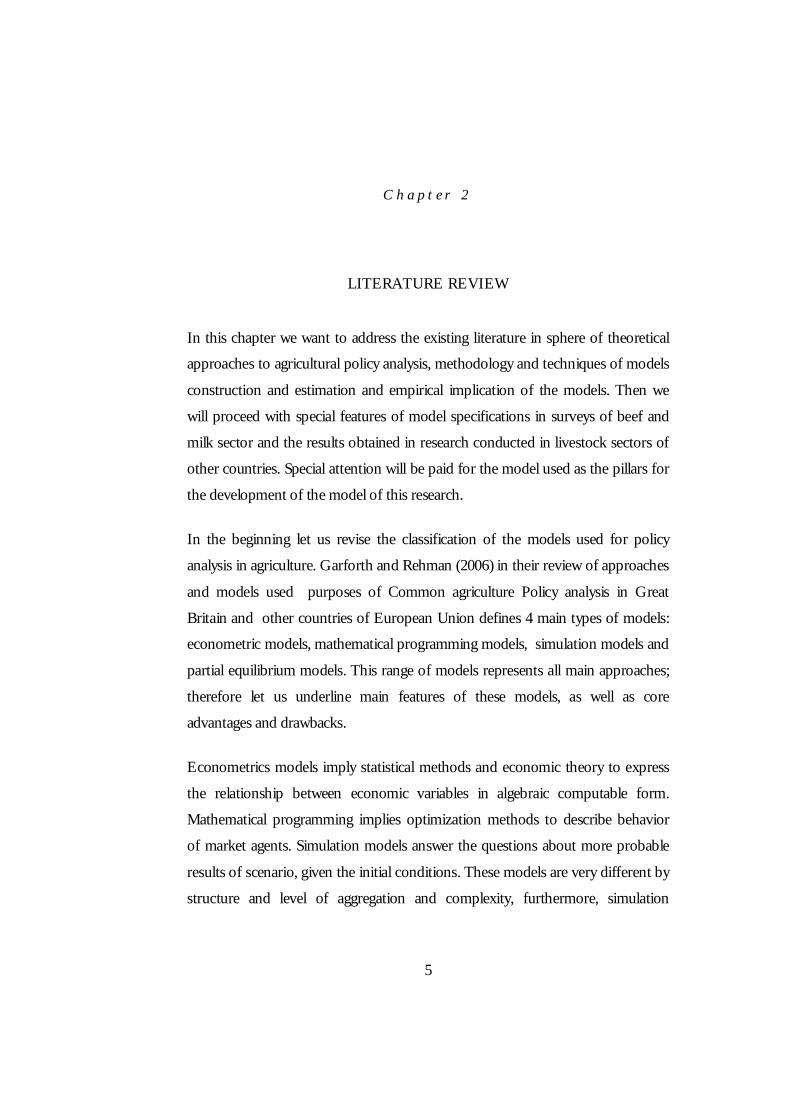
Graph 4.3 Net trade in milk and dairy goods Net trade in milk and dairy goods, tons/month
-100000
-50000
0
50000
100000
150000
200000
250000
300000
350000
Jan 200
3
July 200
3
Jan 200
4
July 200
4
Jan 200
5
July 200
5
Jan 200
6
July 200
6
Net trade in milk and dairygoods
3.2. Protection and Domestic support of the livestock sector. As the main agricultural commodities, beef and milk sector in Ukraine is
protected by the import tariff rate. Tariff rate for beef is 10%, but not less than
10 EUR/tone, tariff rate for raw milk is 10%, but not less then 10 EUR/tone, for
dairy products the tariff rate varies from 10% to 40%. For the purposes of
analysis I calculated weighted average on the trade data of 2006 – 27%.
3.3 The WTO agricultural conditions, predicted risks and benefits
for Ukraine
In the process of discussion of WTO accession of Ukraine, experts (here I
refer to Ostashko T (2002), (2004), (2006), Nivjevsky (2004) and Kobuta (2005))
underline the benefits from market liberalization as well as risks for domestic
producers. Among the main question of concern is domestic market
liberalization, which is expected to weaken the positions of domestic producers.
Furthermore, this weakening is expected to be catalyzed by implementing of new
sanitary and phyto-sanitary standards defined in the Agreement on Agriculture,

14
and as a result by increasing production costs of domestic producers. State
support reduction consider to be efficient, as well as free trade will benefit market
efficiency and budget burden will switch to the rural development and
improvement of quality of goods produced. Market institutions development is
expected to be reinforced; structure of agricultural producers will change towards
decline of small and medium enterprise production share in total production.
Trade shocks will also become less possible after WTO accession.
It can be forecasted on the base of transition economies experience, that
state support of agriculture will restricted mainly by the budget constraints, not
be the WTO requirements.
Without any doubts, rural development will benefit from WTO accession,
as well as quality of goods produced and consumed, however, influence of
implementing WTO requirements and restrictions on the each goods should be
analyzed separately.
While analyzing the level of import tariffs for particular goods, the results
of survey appears to be controversial. Thus, Nivjevskiy in his survey of ability of
domestic goods to compete on the domestic and world market conducted in
2004 argues, that almost all goods will remain in their initial positions after
reduction of import tariff. From the other hand, Ostashko T (2006) argues, that
Ukraine shows tendency of agricultural and food import growth after changes to
the Custom tariff in July 2006 (during first half of 2006 import of these items
increased by 26,6% in comparison with the same period of 2005).
By this thesis I want to some extent contribute to the forecasting and
estimation of tariff reduction consequences for the case of milk and beef.

15
C h a p t e r 4
THEORETICAL CONSIDERATIONS: PARTIAL EQUILIBRIUM MODEL AND WELFARE ANALYSIS
4.1 Theoretical framework developing
According the discussion of Chapter 2, it can be concluded that partial
equilibrium model is the most feasible tool for our analysis. The model will
provide us with the framework for equation specification and static relationship
analysis that will further be included into simulation model.
The following assumptions are to be implied before describing the
framework:
Ø Ukraine is a small country, and the level of its export and import
of the goods analyzed does not affect the world price
Ø Goods are homogenous, therefore import and domestic goods
compete only by price, not by the means of consumer preferences
Ø Producers and consumers behavior rationally – producers
maximize their profitability, consumers maximize their utility with
budged constraints.
Ø Transportation costs and transactions costs assumed to be equal
for imported and domestic goods.

16
These assumptions, extent of their impact on the model results and
forecast of the consequences of realizing these assumptions are presented at the
end of this Chapter.
Therefore, the market equilibrium model is described as follows:
For each good i, included in the model,
Domestic Demand:
),,,( )(,, ddotherdidd
id uIPPFQ = Equation 4.1.
Domestic Production:
),,,(
)(,, prprotherpriprd
ipr uIPPFQ = Equation 4.2.
with
Qdd stays for level of domestic demand of good i
Qdpr stays for domestic production level of good i
Pd,i – market price of the good i Ppr,i – producers price of the good produced (price at which producers supply goods to the market) Id – vector of exogenous variables that influence demand, for example, income per capita etc Ipr – vector of production factors prices Ud and Upr – disturbances.
The difference in production vector of primary goods produce and
proceeding goods will be discussed in model specification in Chapter 5.
The closure of our partial equilibrium model includes price equilibrium
conditions and net trade equations. As statistical data on the net trade is collected
together for both raw milk and dairy products, and no separate data is available,
only two net trade equations will be included into our model as a closure.
That is, for every good i :

17
Pd,I = Ppr,I Equation 4.3. Qd
pr - Qdd =NTi
With NTi describing the net trade level in good I
4.2. Analysis of reduction in production subsidies In this Section we will briefly address static graphic analysis of welfare
effects of government intervention, terms of trade and trade shocks. Figure 4.1. Welfare analysis under production subsidies reduction Source: Perali (2002)
The consequences of reduction of production subsidies for the case when initial
and resulting equilibrium prices are above the level of equality of domestic supply
and demand, are presented on the Figure 1. With reduction of subsidy, the
production curve shifts up, therefore, equilibrium price increases, while market
clearing level of net trade decreased. For the purposes of our analysis, we assume
that net trade and domestic demand reacts by the same extent to changes in
prices. This assumption is true for Ukraine as the small country, and the fact that
P1
Q
Qs 0
Qs1
Qd 0
P2
P
Qd Qc
A B
C D
Qa Qb
1 2 4 3 5 6
7

18
Ukraine exports not at the level of the world prices (See Section 4.1. for
reasoning).Therefore, the domestic demand declines from the level of Qc to the
level Qa, the net trade level declines from (Qd-Qc) to (Qb-Qa). Level of production
changes from Qd to Qb.
The table below presents the welfare consequences of subsidy reduction:
Table 4. 1. Welfare analysis under reduction production subsidies Welfare estimator Direction of Change Value of change Change in consumer surplus Decline 1+2 Change in producer surplus Increase 1+2+3-5-6-7 Change in government costs/revenue
Decline in costs 5
Total welfare effect (-1)+(-2)+1+2+3-5-6-7 +5 =3-6-7
Note: Figures, which squares reflects the change in welfare presented on Figure 1. For this and others graphical analysis of this chapter, algebraic calculations
of welfare changes are presented in Appendix 1B.
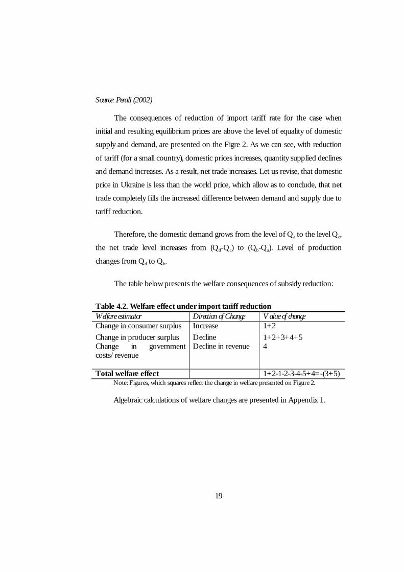
4.3. Import tariff reduction and welfare effects Figure 4.2. Welfare effect under import tariff reduction
P2
Q
Qs 0
P1
P
P2
Q
Qs 0
P1
P
Qd Qc
A
C D
Qa Qb
P2
Q
Qd 0
P1
P
1 2 4
3 5 B
19
Source: Perali (2002)
The consequences of reduction of import tariff rate for the case when
initial and resulting equilibrium prices are above the level of equality of domestic
supply and demand, are presented on the Figre 2. As we can see, with reduction
of tariff (for a small country), domestic prices increases, quantity supplied declines
and demand increases. As a result, net trade increases. Let us revise, that domestic
price in Ukraine is less than the world price, which allow as to conclude, that net
trade completely fills the increased difference between demand and supply due to
tariff reduction.
Therefore, the domestic demand grows from the level of Qa to the level Qc,
the net trade level increases from (Qd-Qc) to (Qb-Qa). Level of production
changes from Qd to Qb.
The table below presents the welfare consequences of subsidy reduction:
Table 4.2. Welfare effect under import tariff reduction Welfare estimator Direction of Change Value of change Change in consumer surplus Increase 1+2 Change in producer surplus Decline 1+2+3+4+5 Change in government costs/revenue
Decline in revenue 4
Total welfare effect 1+2-1-2-3-4-5+4=-(3+5)
Note: Figures, which squares reflect the change in welfare presented on Figure 2. Algebraic calculations of welfare changes are presented in Appendix 1.
20
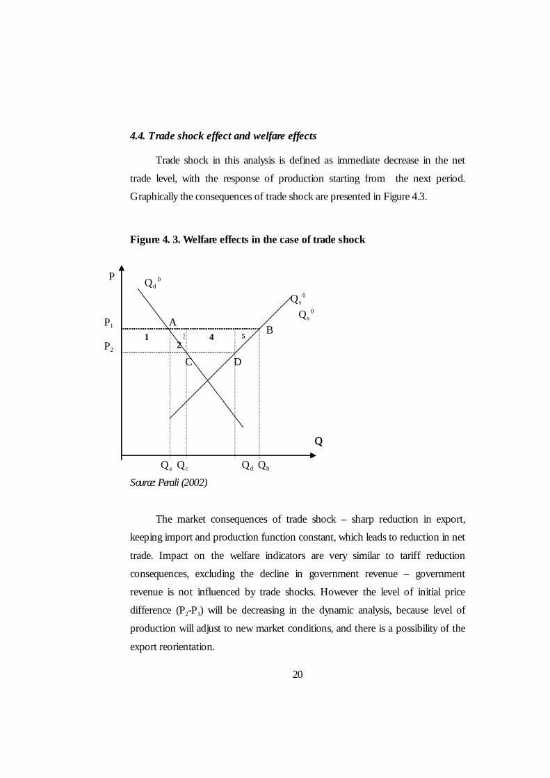
4.4. Trade shock effect and welfare effects
Trade shock in this analysis is defined as immediate decrease in the net
trade level, with the response of production starting from the next period.
Graphically the consequences of trade shock are presented in Figure 4.3.
Figure 4. 3. Welfare effects in the case of trade shock Source: Perali (2002)
The market consequences of trade shock – sharp reduction in export,
keeping import and production function constant, which leads to reduction in net
trade. Impact on the welfare indicators are very similar to tariff reduction
consequences, excluding the decline in government revenue – government
revenue is not influenced by trade shocks. However the level of initial price
difference (P2-P1) will be decreasing in the dynamic analysis, because level of
production will adjust to new market conditions, and there is a possibility of the
export reorientation.
Q Q
Qc
C
3P2
Qs 0
P1
Qs 0
Qd
A
D
Qa Qb
Q
Qd 0 P
1 2
4 5 B

21
Therefore, the net trade level increases from (Qd-Qc) to (Qb-Qa), as a result
production declines from the Qb to Qd, supply on domestic market increase (
form Qa minus the level of import to Qc minus the level of import), the
domestic demand grows from the level of Qa to the level Qc,.
The table below presents the welfare consequences of the trade shock:
Table 4. 3. Welfare effects in the case of trade shock 20 Welfare estimator Direction of Change Value of change Change in consumer surplus
Increase 1+2
Change in producer surplus
Decline 1+2+3+4+5
Change in government costs/revenue
Decline in revenue
Total welfare effect 1+2-1-2-3-4+4 = -(3)
Note: Figures, which squares reflect the change in welfare presented on graph. Algebraic calculations of welfare changes are presented in Appendix 1.
4.5. Nerlovian coefficients
In this section I will discuss the Nerlove theory of partial adjustment for
production, demand and number of livestock functions.
Gaisford and Kerr (2001), Askari and Cummings (1976), More et al (2002)
mentioned that such functions accurately reflects the trends of agriculture
production and primary food demand.
The Nerlove theory is based on the postulate, that producers make their
decision about the desired level of production changes on the base of market
conditions. However, they are not always able to react at the desired level in
practice, therefore, the real level of changes is a part of the desired level. In the
case of livestock sector, we can provide an example, that in the case of price for
22
milk increase, a farmer desires to enlarge its production by 40%, however, by
means of decrease in slaughtering for beef he can increase raw milk production
only by 20%. Further increase is possible only by enlargement of production
capacities – buying of new cows, natural number livestock growth, or
technology/feeding improvement. All these measures requires time and capital
inputs, therefore they could not be implemented in the short-run period. In this
case, the Nerlovian coefficient of partial adjustment will be 0,5.
In the consumers behavior analysis, such partial adjustment can be
explained by the psychological factors, such as subjective consumer preferences
and low level of short-run response to change in market conditions. Furthermore,
in our analysis we consider primary consumption goods, which for some
consumers could not be substituted by other goods, at least in short-run. This
statement is also supported by Seperovich and Shevtsov (2004), in their
theoretical considerations about low elasticity of demand response for change in
market conditions.
Providing the reasons for including the Nerloviann coefficient into
modeling framework, I further proceed with algebraic derivation of the
coefficient.
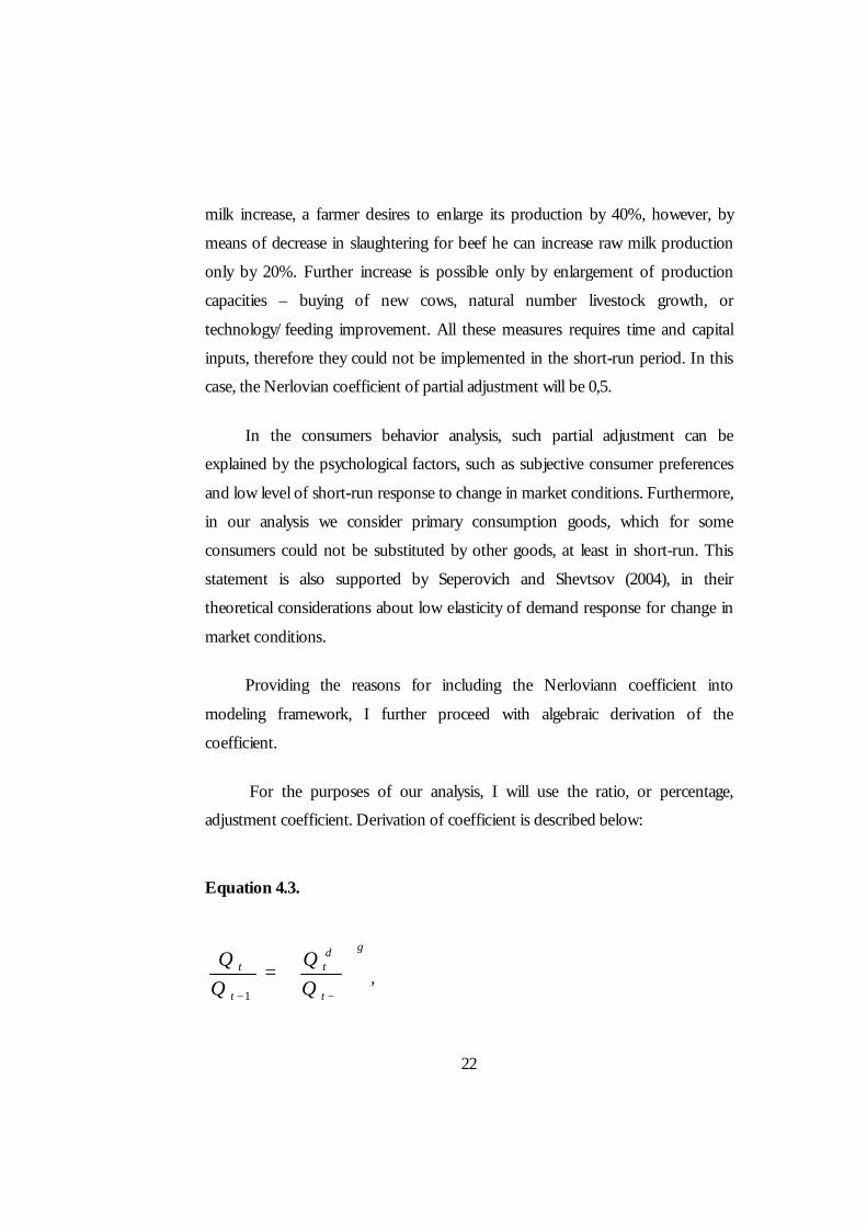
For the purposes of our analysis, I will use the ratio, or percentage,
adjustment coefficient. Derivation of coefficient is described below:
Equation 4.3.
γ
=
−− t
dt
t
t
1,

23
with Qt and Qt-1 – real value of function in period t and t-1 correspondingly, Qt
d – the desired level of function Q. Then, γ reflects the level of adjustment. Equation 4.4.
γ
γ
−−−
−
=
= 1
111
)(*)(* tdtt
t
dt
t QQQQQQ
As far as function specification in Partial Equilibrium model are developed on the
postulates of producers and consumers rational behavior, these specifications
represents the desired level of function. Implementing Nerlove coefficients
methodology via including the lagged value into functions estimated will provide
us with accurate estimation of real value of function.

24
C h a p t e r 5
MODEL SPECIFICATION
5.1. Production function specification
Following the discussions of the previous two chapters, I proceed with
identification of factors that are expected to influence milk and beef producers in
their decision to supply goods to the market.
Here I want to clarify the issue of difference in the terms of production
and supply . Even if supply is calculated as a sum of supplied in domestic market
and exported, nevertheless for case of beef and especially for case of milk not all
goods produced will be supplied. This is mainly caused by the large share of
household production, which have a choice between own consumption and
supply to the market. However, in further specifications we assume that all
production is supplied.
Key determinants of the level of market supply and theoretically expected
relationship with production are presented in Table 5.1.
Table 5.1. determinant of production functions
No Factor Expected relationship with level of supply
1 Price of the good supplied Positive 2 Price vector of production factors Negative 3 Price vector of other agricultural and
food goods indexes Negative
4 Number of livestock at the beginning of the period
Uncertain
5 Level of supply in past period Positive

25
6 Dummy for seasonality (base period – Mar-Oct)
Negative
Coefficients of Price for good supplied and prices of production factors
and their expected relationship with dependant variable are defined by the theory
and need no further discussion. Here I just want to mention that the vector of
production factors includes price for feed and price for labor. Price for labor is
calculated as a wage level index in agriculture and is the part of my database,
described in the beginning Chapter 6. Price for feed is a price index of animal
feeding, collected by the State Statistics Committed. Intuitively, here could be
included three more production factors – land, capital and energy sources.
However, as the majority of agricultural producers obtained the land and capital
buildings as a share after reforming the collective farms, or the land with
buildings in the long-term rent, and, furthermore, agriculture land could not
legally be an object of trade, I did not include this factor into my analysis. Energy
sources price are among the most significant for agriculture production, however
its impact expected to be much lower for livestock than for crop production.
Therefore, price for energy impacts the level of production via price for feed, and
don’t need to be included into the model as a separate factor.
Prices vector of other agricultural and food goods is defined as following:
Ø price index of other (not beef and milk) primary livestock
products,
Ø price index of crop production for primary consumption,
Ø price index of basic processed agricultural goods
Ø cross-good prices, therefore price for milk for beef production
equation and vice verse.

26
Number of livestock at the beginning of the period is included with
purpose to reflect the relationship between beef and milk production. This will
benefit for simplification of estimation process. However, the direction of this
variable’s impact on production is currently uncertain, and it will be discussed
below.
Level of supply in previous period reflects the partial response of supply to
market structure changes (I refer here to Nerlovian coefficients discussion in
Chapter 4).
Dummy variables is included to capture the effect of seasonality of
production which is explained by specifics of agriculture (see Chapter 3). Base
period for dummy is March-October.
The specification of the production of the second level of vertical
aggregation – dairy production function, is a little different from specification of
the function of primary agriculture goods production. Again, referring
ERS_PENN model described by Abler and Stout (2004) and other sources, the
following factors are expected to influence the level of production:
Table 5.2. Determinants of Dairy production function No Factor Expected relationship
with level of supply 1 Price ratio (price of dairy/price of raw
milk) Positive
2 Price vector of production factors Negative 3 Level of production in past period Positive 4 Dummy for seasonality (base period –
Mar-Oct) Negative
Firstly I would like to note, that level of production is assumed to depend
upon level of profitability (expressed as the price ratio variable). In order to avoid
multicolinearity, dairy price is not included in the model.

27
Price vector of production factors consists of price for labor (average wage
in industry index) and energy price index.
In this case, the relationship of dependant variable with the level of
production in past period expected to be significant and the coefficient is
expected to be higher that 0,5, because the technology and capital equipment of
dairy production could not be shifted to other goods production in short-term.
5.2. Specification of demand equations
Following the discussions of the previous two chapters, I proceed with
identification of factors that are expected to influence raw milk final demand,
dairy demand, and beef demand. The demand for milk for processing requires
separate discussion, and will be discussed later un this Chapter.
According to theory and surveys of agriculture demand determinants
conducted by Seperovich and Shevtsov in 2004 and More et al in 2002, the key
determinants of the level of demand are the following: price of good, price for
substitutes and supplements (if appropriate for the good analyzed), level of
income per capita (expected level, sign and significance depends upon the nature
of good, in our case, for beef and dairy income elasticity is expected to be positive
and significant, for milk insignificant or very low) and other reasons such as
consumer preferences, share of rural/urban population, cultural reasons, etc. The
last reasons listed will not be estimated separately in our analysis, because they are
outside of targets of this research, their impact in our case will be represented by
Nerlovian coefficient (see discussion in Chapter 4). The own price elasticity is
expected to be in the interval (0,2-0,4); expected level, sign and significance of
income elasticity depends upon the nature of good. Income elasticity for beef and
dairy is expected to be positive and significant, for raw milk it is expected to be
insignificant or very low)

28
The discussed factors that influence raw milk final demand level, beef
demand level and dairy demand level together their expected relationship with
demand functions are listed in Table 5.3
Table 5.3. Determinants of demand functions No Factor Expected relationship with level of
demand 1 Price of the good Negative, in interval (-0,2) – (-0,40 2 Price vector of goods-
substitutes Positive
3 Income per capita Positive (insignificant for raw milk final demand)
4 Level of demand in past period
Positive in interval (0,5)-(0,7)
In the process of model estimation I will check the hypotheses stated in the
above table.
Further in this section I will proceed with specification of demand of raw
milk for the purposes of processing. As stated in Stout and Abler (2004),
industrial demand for raw milk depends upon the expected level of dairy
production, this dependence is linear until the technology is not changed.
Therefore, on the base of the statistics of milk demand for dairy production
presented by the Association of Dairy Producers of Ukraine, I finish up with the
following specification of demand for milk for processing:
Dprocmilk = 1,27 PrDairy, Equation 5.1 With Dprocmilk - industrial demand of raw milk, and PrDairy – level of
dairy production.

29
The estimation of the specified equations is presented in Chapter 6.
5.3 Number of livestock equation specification In this section I will address
the specification of the number of livestock equation. This equation estimates a
base and restrictions for production of beef and raw milk, as well as the
performance of livestock sector in general (further discussion of number of
livestock as an indicator of agriculture sector performance will be discussed in
Chapter 7). In our analysis we use the term livestock only for livestock used for
milk and beef production.
The decision of producers about the number of livestock depends upon the price
of goods produced from livestock and production factors prices . Also we include
Nerlovian coefficient in the model. The hypotheses of this coefficient are the
following:
Ø it is statistically significant (nature of livestock keeping supports
this, and furthermore, livestock increases by reproducing itself)
Ø it is possible that Nerlovian coefficient here is higher that 1,00. If
it is higher, this means that market conditions do not prevent
natural increasing of the livestock.
Factors that influence the number of livestock and the expected relationship of
these factors with the number of livestock are presented in the Table below
No Factor Expected relationship with level
of demand 1 Price of milk Positive 2 Price of dairy Positive 3 Price of beef Both sided, therefore can’t
be expected without estimation

30
4 Level of livestock by the end of the last period
Positive and could be higher than 1
5 Price for production factors Negative
Some factors and the relationship between factors and dependant variable
are not obvious from the theoretical point of view, therfore I will proceed with
providing some reasoning for them. Price for dairy is included in the model as a
factor of goods produced due to existence of farms aggregated with the
processing facilities. They do not supply raw milk in the market, however they
produce and supply dairy, and their decision on the number of livestock keeping
depends upon the price for dairy.
Price of beef influence the number of livestock in both sides – a farmer can
decide to produce more in this period, while the price is high, an therefore the
number of livestock will decline. From the other point of view, farmer can decide
to accumulate livestock according to rational expectations of further price
growth. Therefore, currently the expected relationship is uncertain.

31
C h a p t e r 6
MODEL ESTIMATION
6.1. Data description.
Data was collected by State Statistics Committee of Ukraine and the United
Nations Development Project (Agricultural Database) and processed by the
author.
The data describes the livestock market of Ukraine, therefore it was
analyzed in the market analysis in Chapter 2.
The data which I use to construct the database for this research was
monthly for the period of January 2000 till March 2007.
The processing of data includes the following: adjustment of the level of
income by CPI, constructing price indexes and labor price indexes.
Section The 2SLS models estimation procedure, chosen with the purpose
to solve the problem of endogeneity in the model, reported statistically significant
results for all equations. Furthermore, initial OLS estimation (estimation output
presented in Appendixes 3-10), while having a difference from 2SLS results in the
value of coefficients, is consistent with 2SLS in the direction of relationship.
Here we don’t use 3SLS or GMM for estimating the model, as it is not
necessary for the purposes of our analysis, however it must be done, if more
detailed or wide research is conducted. Brief analysis of the possible robustness
of estimation by 2SLS comparatively to 3SLS is presented at the end of this
chapter.

32
Below I will proceed with the results of 2SLS estimation of the functions.
The results of 2SLS estimation of production of beef, milk and dairy
equations are presented below in Table 6.1, Table 6.2, Table 6.3. Tables includes
only statistically significant variables, while for the results of regression on all
variables listed as the predictors in Chapter 5 I refer to Appendix 3-10. Some
discussions and reasoning on both significant and insignificant variables and
comparison of their signs and values with expected are provided later in this
section.
6.2. Livestock equation estimation results
In this section I will present results of number of livestock equation
estimation and some discussion behind these results
The table below includes only statistically significant coefficients, for
detailed estimation output I refer to Appendix 8.
Table 6. 1. Livestock number equation estimation results.
No Predictor Coefficient and
significance level 1 Price for beef -,208
(,016) 2 Price for raw milk ,039
(,101) 3 Number of livestock in the beginning of
the period 1,152 (,000)
5 Constant Exp(,153) (,626)
R2 = 0,982 F=766,619 Firstly, I want to mention, that Price for Dairy appears to be insignificant,
that means that either share of joint farms and proceeding plants is low, or they
also make the decisions about level of production on the base of raw milk prices,

33
for example if processing production facilities productivity if higher, than farm
milk productivity, and producers have to buy additional raw milk for the
purposes of production process.
Price for beef is negatively related to the number of livestock, therefore, we
conclude, that maximization of profit in current period are more important for
farmers than expected profitability level (they decide to slaughter for beef, instead
of accumulation of livestock in order to increase the future production level).
Raw milk price elasticity sign is expected, while level if rather low. Again,
this supports the idea that future profitability level is not so important in farmers
decision-making. As increasing of milk production could not be done
immediately due to restrictions of available livestock, farmers do not increase the
livestock for possible future proficts.
Nerlovian coefficient of the equation is higher than 1,00. That means, that
keeping all other market parameters constant, number of livestock will increase.
This allows us to conclude, that applying protection instruments to the livestock
sector will gives it possibility to develop, and therefore be efficient
6.3. Production functions estimation results
Table 6.2. Raw milk production Function estimation results.
No Predictor Coefficient and significance level
1 Price for raw milk ,512
(,001) 2 Production of milk lagged -
3 Price for feed -,905
(,000) 4 Dummy for seasonality -,354
(,000)

34
Number of livestock at the beginning of the period
-,348 (,007)
5 Price index (all agricultural goods) 1,583 (,000)
5 Constant Exp(11,425) (,000)
R2 = 0,865 F=23,278 Note: level of significance is in parenthesis Level of raw milk production is insignificant in the reports of all
methodologies I used to estimate the functions. This result is surprising, because
it shows that Nerlovian coefficient of raw milk production equals 1 and
production is absolutely elastic to market changes. However, this statement is
partially controversial, because the coefficient of the number of livestock in the
beginning of the period is significant. Furthermore, logically milk production
depends upon the number of livestock. As we saw in the previous section of this
Chapter, the Nerlovian coefficient of the number of livestock is significant and
even higher than 1, therefore, the elasticity of raw milk production is restricted by
the low level of respond of the number of livestock. Furthermore, coefficient of
the number of livestock variable is negative, which can be explained by the fact,
that while farmers are increasing the livestock, they use raw milk for the purposes
of feeding, and therefore, number of supplied production decreases
Elasticity coefficient of price for raw milk and dummy variable coefficient
obtained support the hypothesis about sign and value.
Cross-price elacticity (here presented by the coefficient of price index for
all other agricultural goods) shows surprising results in sign and level. A possible
explanation of this could be the decision-making process about enlargement of
agricultural enterprises and increasing/decreasing number of these enterprises.
For example, if agricultural price index is growing, producers are more stimulated
to attracting more capital (crediting is included) and labor into the enlargement of

35
their production level on the base of expectations of increasing profitability. The
same logic lies behind the creating of new farms. As the processes of production
of agricultural goods are interrelated, usually the production of goods increased
simultaneously.
When analyzing the impact of production factors prices, we could see that
the theoretical expectations are not satisfied – price for feed is more significant
than price for labor. However, production of milk is rather labor-intensive than
feed-intensive. A possible explanation of this is as following: due to high level of
rural unemployment and lack of other employment possibilities for farm-workers,
the influence of average wage proposed on the decision of whether to supply
labor force in labor market or not is not so significant as supposed by the theory.
Feed is competitively traded in the market, therefore its price and number
supplied is influenced by market forces, therefore it more likely influences the
level of production as a production factor price.
Table 6.3. Beef production function estimation results
No Predictor Coefficient and significance level
1 Price for beef ,695 (,142)
2 Number of livestock at the beginning of the period
-1,448 (,006)
3 Price for raw milk -,827 (,000)
4 Price for labor ,814 (,000)
5 Dummy for seasonality - 6 Constant Exp (19,793)
(,000) R2 = 0,570 F=14,243
Note: level of significance is in parenthesis
All coefficients obtained (except price of labor coefficient) support signs
and values expected on the base of theory and methodology. Insignificance of
36
dummy variable is compensated by the significance of prices for beef (however,
the level of its significance is surprisingly low), because price for beef is more
periodically fluctuated than the price for milk (I refer to Chapter 3 for reasoning).
A possible explanation of higher significance of cross-price elasticity
coefficient the own-price elasticity (raw milk and beef correspondingly) could be
explained by perfect substitution of milk and beef (but not vise versa) in
production process. If a producer decides to decrease the production of milk, he
has to decrease the number of milk livestock, which results if increase in beef
production. Note that vice versa dependence is not so direct, therefore the
production of raw milk is not significantly influenced by prices for beef.
Explanation for number of livestock coefficient is obvious: beef is
produced via slaughtering the livestock, consequently the lower is the number of
livestock, the less beef could be produced.
Positive significant coefficient of price for labor contradicts theoretical
expectations about the sign. However, if we consider that increase in production
of beef leads to decrease in number of livestock, and therefore, to decline in the
labor necessary for livestock keeping, we can conclude, that expectations of
increase in labor price will positively effect the level of beef production.
Furthermore, based on the theory of rational expectations, the increase in current
price for labor will develop of expectations its of further growth. According to
this explanations, positive sign of the coefficient could not be treated as biased
statistical estimation.
Nerlovian coefficient appears to be insignificant (see Appendix 4), that can
be explained as for the milk production – its effect is captured by the livestock
number variable coefficient.

37
Table 6.4. Dairy production function estimation results
No Predictor Coefficient and
significance level 1 Price ratio 2,162
(,000) 2 Production of dairy lagged ,164
(,224) 3 Price for labor (industrial) -,045
(,064) 4 Constant Exp (7,573)
(,000) R2 = 0,745 F=40,281
Notes: price ratio stays for ratio of prices of raw milk to dairy products prices level of significance is in parenthesis
As it was expected, the coefficient of price ratio variable that reflects the
profitability of production is significant and its value is high. This supports the
theoretical background after the behavior of agriculture processing industry
producers.
Also the significance of Nerlovian coefficient (which is low, but still allows
rejecting the hypothesis, that coefficient is statistically zero) provides as with
conclusions, that dairy production function is a partially responding function.
Furthermore, the level of Nerlovian coefficient is 0,164, therefore, real response
of dairy production to the market changes is equal 1 – 0,164 = 0,836, i.e. 83%.
This level is rather high, and the possible explanation for this is that producers
can decrease their production, however, they are not able to re-orient production
facilities to other goods production. From the other point, producers are able to
increase production level, because their production facilities are not used at all
capacity (as noted by the Head of Dairy Producers Association of Ukraine, see
Kobuta (2006), however increase of production capacity will require capital
inflow and/or technological changes. These reasons explain why the dairy

38
production is partially responding, but the level of immediate response is rather
high.
Price for labor coefficient supports theoretical hypothesis about sign and
significance. The Seasonal dummy variable was not included into analysis,
because the production process of dairy do not depends on the seasonality, as
agricultural production do (producers has stocks of dry milk produced from raw
milk and ensures the stable level of production through the year).
In this section we discussed results of production functions estimation by
the 2SLS procedure. In the next section we will proceed with presentation and
discussion of demand functions estimation, and further the whole obtained
model including the partial equilibrium closure conditions will be presented.
Section 6.4. Demand functions estimation
In this section I will present results of demand equations estimation and
some discussion behind these results
As for the production function estimation, the tables below include
statistically significant coefficients, and, some of statistically insignificant but
important for our discussion. For detailed estimation output I refer to
Appendixes 7,6,9.
Table 6.5. Demand for beef Function estimation results.
No Predictor Coefficient and significance level
1 Price for beef -,549 (,007)
2 Income per capita ,480
39
(,000) 3 Price index (all agricultural goods) ,476
(,099) 4 Price for raw milk -,610
(,000) 5 Constant Exp (13,934)
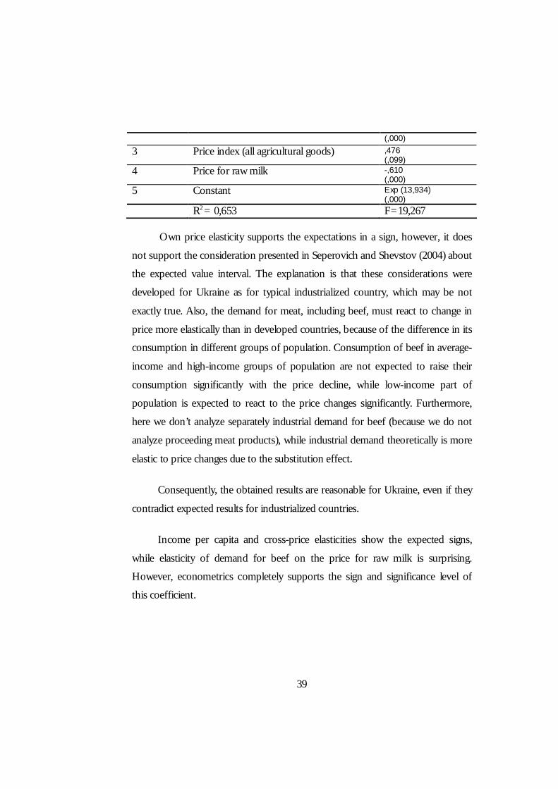
(,000) R2 = 0,653 F=19,267
Own price elasticity supports the expectations in a sign, however, it does
not support the consideration presented in Seperovich and Shevstov (2004) about
the expected value interval. The explanation is that these considerations were
developed for Ukraine as for typical industrialized country, which may be not
exactly true. Also, the demand for meat, including beef, must react to change in
price more elastically than in developed countries, because of the difference in its
consumption in different groups of population. Consumption of beef in average-
income and high-income groups of population are not expected to raise their
consumption significantly with the price decline, while low-income part of
population is expected to react to the price changes significantly. Furthermore,
here we don’t analyze separately industrial demand for beef (because we do not
analyze proceeding meat products), while industrial demand theoretically is more
elastic to price changes due to the substitution effect.
Consequently, the obtained results are reasonable for Ukraine, even if they
contradict expected results for industrialized countries.
Income per capita and cross-price elasticities show the expected signs,
while elasticity of demand for beef on the price for raw milk is surprising.
However, econometrics completely supports the sign and significance level of
this coefficient.
40
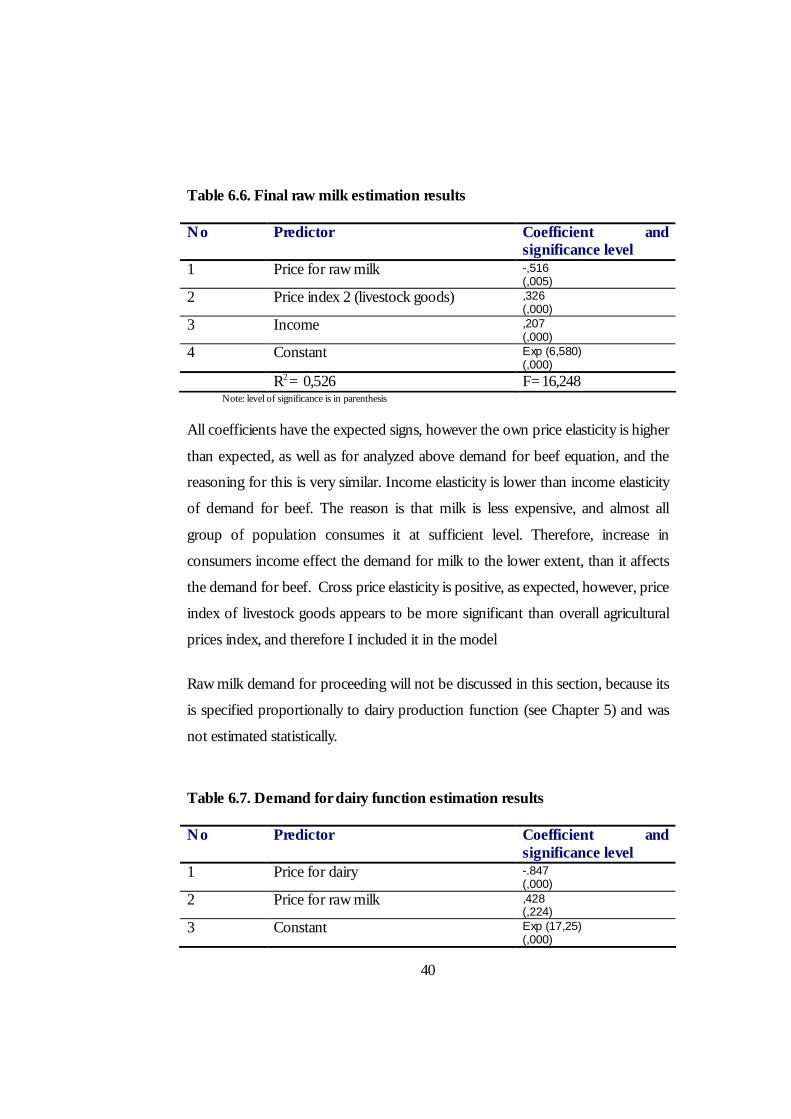
Table 6.6. Final raw milk estimation results
No Predictor Coefficient and significance level
1 Price for raw milk -,516 (,005)
2 Price index 2 (livestock goods) ,326 (,000)
3 Income ,207 (,000)
4 Constant Exp (6,580) (,000)
R2 = 0,526 F=16,248 Note: level of significance is in parenthesis
All coefficients have the expected signs, however the own price elasticity is higher
than expected, as well as for analyzed above demand for beef equation, and the
reasoning for this is very similar. Income elasticity is lower than income elasticity
of demand for beef. The reason is that milk is less expensive, and almost all
group of population consumes it at sufficient level. Therefore, increase in
consumers income effect the demand for milk to the lower extent, than it affects
the demand for beef. Cross price elasticity is positive, as expected, however, price
index of livestock goods appears to be more significant than overall agricultural
prices index, and therefore I included it in the model
Raw milk demand for proceeding will not be discussed in this section, because its
is specified proportionally to dairy production function (see Chapter 5) and was
not estimated statistically.
Table 6.7. Demand for dairy function estimation results No Predictor Coefficient and
significance level 1 Price for dairy -.847
(,000) 2 Price for raw milk ,428
(,224) 3 Constant Exp (17,25)
(,000)

41
R2 = 0,590 F=31,463 Notes: level of significance is in parenthesis
The dairy demand function estimated results appears to be the simplest
one, and they completely support theoretical considerations. Own price elasticity
value is rather high, because dairy is a processed good with almost perfect
substitution effect of the unprocessed input – raw milk. That is why, consumers
in case of price increase substitute dairy products with raw milk, especially in rural
areas. This substitution effect could also be a reasoning for rather high level of
cross-price elasticity. As milk and dairy are first-necessity goods, income elasticity
coefficient appears to be insignificant. Therefore, it could be concluded, that in
case of income per capita reduction, consumers shift from milk consumption to
dairy consumption, and the income elasticity effect is statistically represented in
own-price and cross price elasticity.
Furthermore, these estimation results remind us about the problem of
endogeneity between demand for milk and demand for dairy. In the case of 3SLS
estimation procedure, we could obtain different and more accurate results,
including the significance of coefficients. However, it is a proposition for a
further research.
Summarizing this section I would like to underline, that none of the
Nerlovian coefficients in final demand functions appear to be significant. That
means, that for the case of beef, milk and dairy the demand is completely
adjusted to market changes.
6.5. Assumptions analysis.
In this section we will discuss the role of assumptions in our model and the
approaches to estimate the bias caused by them. In the Chapter 2 we mentioned

42
that econometrically estimated models are usually the most vulnerable to the
assumptions defined. In our case assumptions are questioned by including non-
homogenous producers into our model: we discussed large farms, small farms
and households producers in one equation estimated.
The first assumption of our model states that all producers’ behavior is
determined by the profit-maximization principle. The literature supports this
assumption for developing of econometric models. However, in our estimation
this assumption is suspected to bring a significant bias due to large share of
household producers, which at the same are factor suppliers for production.
Hence supply function estimation may face a problem of non-homogenous of
supplier’s behavior.
For example, household production, and furthermore the decision to
supply production to the market, is influenced by variety of other factors, such as:
level of employment, wage in agriculture, income per capita, level of uncertainty,
rural development and infrastructure. There appears a possible bias in the
production function estimation. The most efficient way to release this assumption
is to develop 2 separate production equation and, possibly, livestock number
equation – for farms-producers and households producers. However, we will not
construct these 2 equations in order to keep our model estimable, nut instead we
will try to analyze the possible bias in the process of production equation
estimation.
One of the most significant assumption of econometric models estimation
is constant relationship, i.e. coefficients of production function are constant
through period of data used for estimation. This does not capture the possibility
of technological changes. However, based on the agriculture enterprises survey in
2005 in Ukraine, conducted by Ostashko (2004) the producers mentioned, that
there were no significant improvement in technologies during 2000-2005.
43
Therefore, this assumption is realistic and econometric approach to policy
analysis suits the case of Ukrainian livestock sector.
Other assumption concerning the producers is their equal access to
exporting possibilities. This is definitely not real, but taking into account well
grounded assumption of goods homogeneity in domestic market (realistic for the
case of Ukraine) we will just assume that goods produced by households that are
desired to exported are substituted with the goods produced by farms, while
domestic market is a little shift to the higher share of household producers.
In a difference from our case, European studies Bienfield (2003) and
Meinke (1999 pay more attention to bias caused by assumptions of consumer
side. A lot of discussions of are around of assumption of import-domestic goods
level of substitutability. It means, that the competition of these goods is not
determined only by price, but also by some transparent or hidden factors of
consumer preferences. In some models, for example in IMPACT and ERS-
PENN models (see Chapter 2) special coefficient of substitution is included.
However, we consider, that beef and milk (especially the last one) market is
sufficiently homogenous for our analysis. One of the features of milk and dairy
sector in Ukraine is high share of goods produced by joint or multinational
companies. These companies usually have their departments in Ukraine and in
main trade partners of Ukraine. Therefore, historically Ukrainian milk and dairy
market is not distorted by subjective preferences between domestic and imported
goods.
6.6. Considerations on 3SLS estimation procedure
By means of conduction 2SLS procedure we obtain more accurate
estimation of coefficients, than would obtain is using OLS. We use and

44
assumption of endogeneity between production and prices, demand and prices,
production and number of livestock, demand and number of livestock.
In the begging Chapter 5 I presented how the possibility of endogeneity
between left-side variables (production and demand variables) of different
equations is addressed in the model specification.
However, in this Section I want to come back to this problem again and
discuss it from the point of view of statistical criteria. Therefore, this paragraph is
devoted to the question if 2SLS estimation was significantly less accurate than
estimation of 3SLS.
I used test for endogeneity, developed on the base of Hausman test. The
procedure was as follows: I conducted the OLS estimation of endogenous left-
side variables on the base of all exogenous variables in the model (one by one).
Obtained predicted values and residuals were included in the set of predictors of
other endogeneity variables. The results presented in Appendix 3. As they show,
we can consider non-significant problem of endogenously between Production
and Demand for Milk - the t-test shows the significance of coefficient of
residuals.
This problem should be addressed separately, however, as these variables
do not appear in our model in one equation, and there is no endogeneity between
others left-side variables, we will not use the 3SLS procedure for estimation in
order not to make our analysis too overloaded by statistical estimation.
However, when using model to analysis of scenarios of raw milk market
interventions, this problem and bias that might be caused by it must be taken into
account.

45

46
47
C h a p t e r 7
EMPIRICAL IMPLICATIONS OF THE MODEL TO ANALYZE THE EFFECT OF POLICY INSTRUMENTS AND TRADE CONDITIONS
In this Chapter we will provide the examples of empirical implications of
the model developed in previous Chapter. We will analyze the following scenarios
– reduction in production subsidies, reduction of import tariff and trade shocks.
The analysis will be conducted for separate scenarios of beef and milk markets,
while the welfare analysis will include changes on both markets (as prices of beef
influence the milk market and vice verse).
Special attention will be paid to the trends in number of livestock, as one of
the factors of livestock sector potential. As argue Ostashko T. (2003), decreasing
tendencies in the number of livestock before entering trade organization
eliminated the possibility to develop an export-oriented livestock sector and to
ensure the position of the country as a net importer of livestock goods.
7.1. Reduction in beef production subsidy.
The scenario parameters suppose that the level of production subsidies is
decreased by 20%.
For this condition we estimate – the level of net trade in beef, change in
the market agents’ welfare, and trends of livestock growth.
48
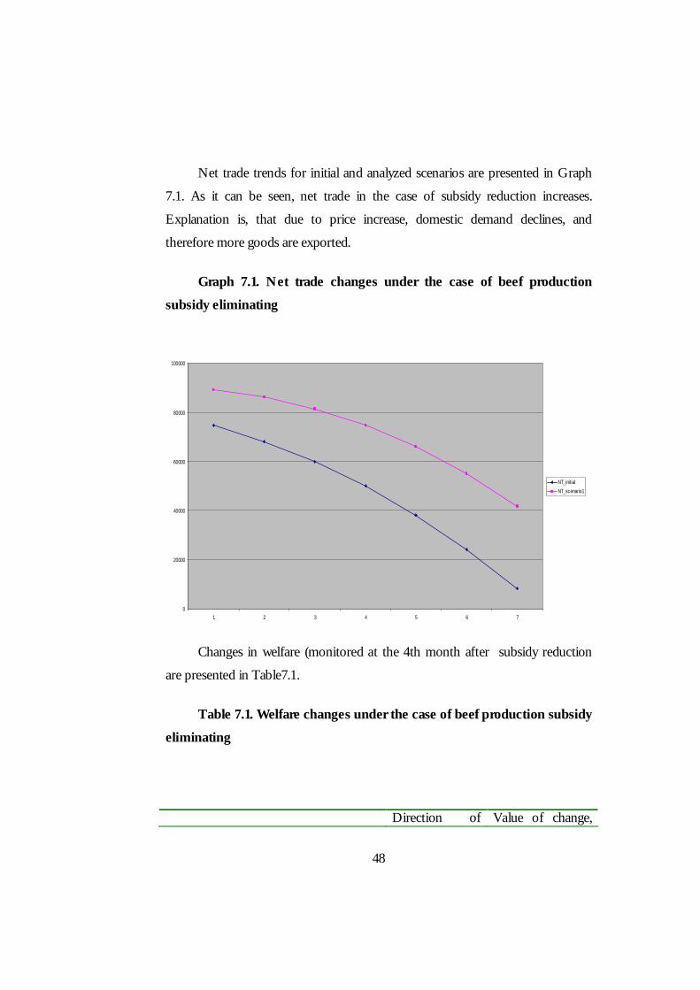
Net trade trends for initial and analyzed scenarios are presented in Graph
7.1. As it can be seen, net trade in the case of subsidy reduction increases.
Explanation is, that due to price increase, domestic demand declines, and
therefore more goods are exported.
Graph 7.1. Net trade changes under the case of beef production subsidy eliminating
0
20000
40000
60000
80000
100000
1 2 3 4 5 6 7
NT_initialNT_scenario1
Changes in welfare (monitored at the 4th month after subsidy reduction
are presented in Table7.1.
Table 7.1. Welfare changes under the case of beef production subsidy eliminating
Direction of Value of change,

49
change mln. UAH Consumer loss change Increase in loss - 480 Producers surplus change Increase 145 Government revenue/cost change Decrease in
costs 3
Total welfare change Negative - 337
Number of livestock is lower than under the basic scenario; however it
shows the growing tendency, as presented n Graph 7.2.
Graph 7.2 Number of livestock changes under the case of beef production subsidy eliminating
6000
6500
7000
7500
8000
8500
1 2 3 4 5 6 7
Stock_baseStock_scenario
Therefore, on the base of this analysis we can conclude that, reduction of
the production subsidy for beef will not contribute to the process of Ukraine
becoming a net importer of beef, while it subsidy reduction will not also prevent
this. The overall tendency estimated in the models shows, that Ukraine in time

50
will become a net importer, however, level of net trade is higher than in the base
scenario.
From the other hand, consumer loss increases, and the total social welfare
changes is negative.
Number of livestock is lower than under the basic scenario, therefore, in
general, it negatively influences the livestock sector development potential.
7.2. Import tax reduction.
As it was argued in Chapter 3, current level of ad valorem import tariff for
beef is 10%, and it does not exceed the marginal level allowed according to the
negotiations between Ukraine and WTO. However, in order to make our analysis
consistent and estimate all scenarios of level of protection change, we will here
analyze the possible decline in import tariff by 5%.
The results obtained are discussed and presented in Table 7.2 and
Diagrams 7.3 ,7.4 below.
Net trade in beef is lower than under base scenario, the trend remains the
same as under the base scenario. Therefore, tariff reduction could possibly
contribute to loosing by Ukraine it position of net exporter in beef.

51
Graph 7.3 Net trade changes under import tariff reduction
-40000
-20000
0
20000
40000
60000
80000
1 2 3 4 5 6 7
nt_initialnt_tariff reduction
Table 7.2 Wellfare effects under import tariff reduction Direction of
change Value of change, mln. UAH
Consumer loss change Decrease 27 Producers surplus change Decrease -167 Government revenue/cost change Decrease in
revenue collected
-0,2
Total welfare change Negative - 140
As can be seen from the above Table, decrease in consumer loss is lower
than production surplus decrease, therefore the total welfare effect of tariff
reduction is negative.
52
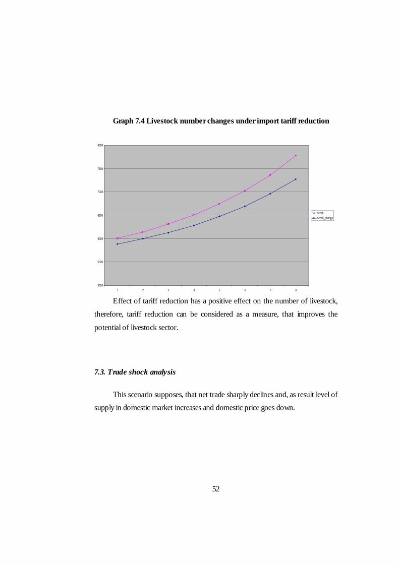
Graph 7.4 Livestock number changes under import tariff reduction
5000
5500
6000
6500
7000
7500
8000
1 2 3 4 5 6 7 8
StockStock_change
Effect of tariff reduction has a positive effect on the number of livestock,
therefore, tariff reduction can be considered as a measure, that improves the
potential of livestock sector.
7.3. Trade shock analysis
This scenario supposes, that net trade sharply declines and, as result level of
supply in domestic market increases and domestic price goes down.
53
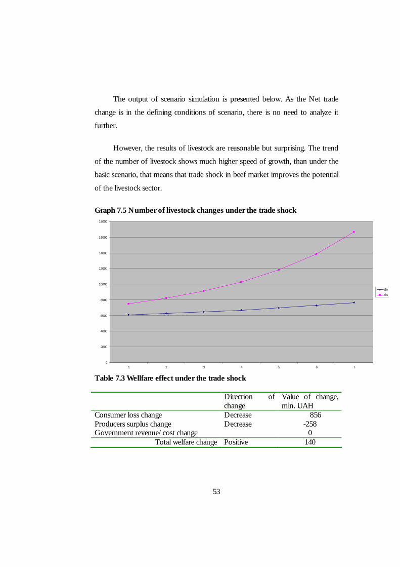
The output of scenario simulation is presented below. As the Net trade
change is in the defining conditions of scenario, there is no need to analyze it
further.
However, the results of livestock are reasonable but surprising. The trend
of the number of livestock shows much higher speed of growth, than under the
basic scenario, that means that trade shock in beef market improves the potential
of the livestock sector.
Graph 7.5 Number of livestock changes under the trade shock
0
2000
4000
6000
8000
10000
12000
14000
16000
18000
1 2 3 4 5 6 7
StockStock_change
Table 7.3 Wellfare effect under the trade shock Direction of
change Value of change, mln. UAH
Consumer loss change Decrease 856 Producers surplus change Decrease -258 Government revenue/cost change 0
Total welfare change Positive 140
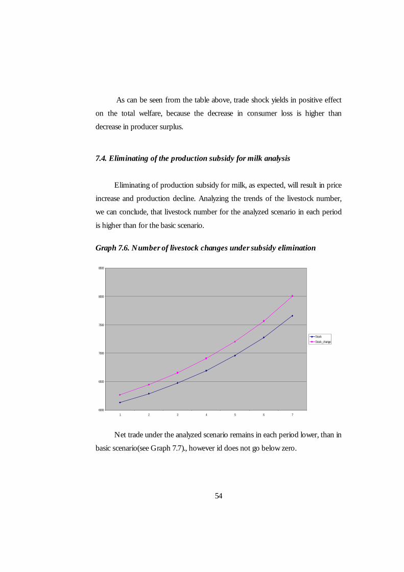
54
As can be seen from the table above, trade shock yields in positive effect
on the total welfare, because the decrease in consumer loss is higher than
decrease in producer surplus.
7.4. Eliminating of the production subsidy for milk analysis
Eliminating of production subsidy for milk, as expected, will result in price
increase and production decline. Analyzing the trends of the livestock number,
we can conclude, that livestock number for the analyzed scenario in each period
is higher than for the basic scenario.
Graph 7.6. Number of livestock changes under subsidy elimination
6000
6500
7000
7500
8000
8500
1 2 3 4 5 6 7
StockStock_change
Net trade under the analyzed scenario remains in each period lower, than in
basic scenario(see Graph 7.7)., however id does not go below zero.
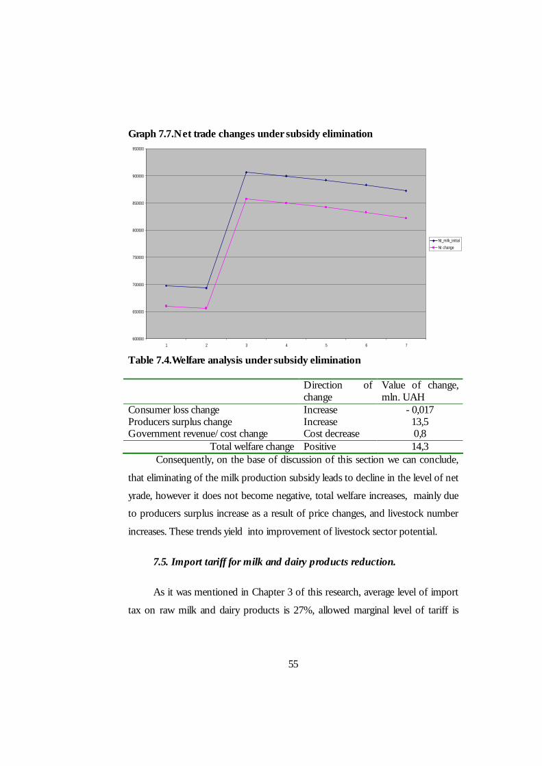
55
Graph 7.7.Net trade changes under subsidy elimination
600000
650000
700000
750000
800000
850000
900000
950000
1 2 3 4 5 6 7
Nt_milk_initial Nt change
Table 7.4.Welfare analysis under subsidy elimination Direction of
change Value of change, mln. UAH
Consumer loss change Increase - 0,017 Producers surplus change Increase 13,5 Government revenue/cost change Cost decrease 0,8
Total welfare change Positive 14,3 Consequently, on the base of discussion of this section we can conclude,
that eliminating of the milk production subsidy leads to decline in the level of net
yrade, however it does not become negative, total welfare increases, mainly due
to producers surplus increase as a result of price changes, and livestock number
increases. These trends yield into improvement of livestock sector potential.
7.5. Import tariff for milk and dairy products reduction.
As it was mentioned in Chapter 3 of this research, average level of import
tax on raw milk and dairy products is 27%, allowed marginal level of tariff is

56
13,5%. Hence, it is useful to simulate and analyze how tariff rate reduction
influences the milk and dairy market
Table 7.5 welfare analysis under import tariff reduction Direction of
change Value of change, mln. UAH
Consumer loss change Decrease +0,013 Producers surplus change Decrease -13,5 Government revenue/cost change Revenue decline -0,2
Total welfare change Negative -13,7 Net trade is lower than the initial level, that is logical due to liberalization of market access for foreign producers. Sharp increase is partially caused by seasonality. Graph 7.8. Net trade changes under import tariff reduction
700000
750000
800000
850000
900000
950000
1000000
1 2 3 4 5 6 7 8
Nt_milk_initial Nt change
Livestock under the scenario analyzed is higher than in the initial scenario,
therefore, reduction in tariff rate improves the potential of livestock sector.
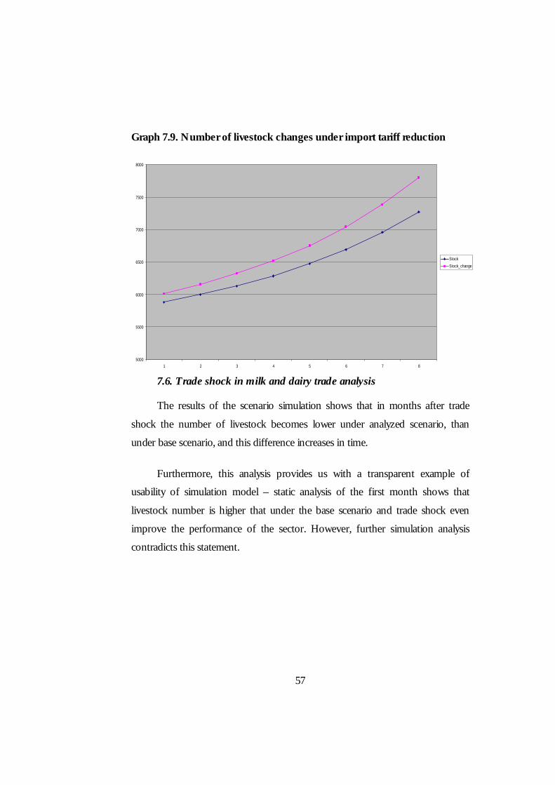
57
Graph 7.9. Number of livestock changes under import tariff reduction
5000
5500
6000
6500
7000
7500
8000
1 2 3 4 5 6 7 8
StockStock_change
7.6. Trade shock in milk and dairy trade analysis
The results of the scenario simulation shows that in months after trade
shock the number of livestock becomes lower under analyzed scenario, than
under base scenario, and this difference increases in time.
Furthermore, this analysis provides us with a transparent example of
usability of simulation model – static analysis of the first month shows that
livestock number is higher that under the base scenario and trade shock even
improve the performance of the sector. However, further simulation analysis
contradicts this statement.

58
Graph 7.10. Number of livestock changes under trade shock
5000
5500
6000
6500
7000
7500
8000
1 2 3 4 5 6 7 8 9
StockStock_change
Table 7.6. The impact of trade shock on the total welfare Direction of
change Value of change, mln. UAH
Consumer loss change Decrease +0,18 Producers surplus change Decrease -127 Government revenue/cost change 0
Total welfare change Negative -127
The impact of trade shock on the total welfare is negative and significant.
Concluding that Chapter I would like to underline that reduction or eliminating
production subsidies on both beef and milk and dairy market leads to improve in
potential of livestock sector, however, influence of these policy measures of total
welfare are different: while reduction of beef production subsidy benefits total
welfare, eliminating of milk production subsidy leads to decline in total welfare.

59
Import tariff reduction in both cases reduces the social welfare, however, it
improves the potential of livestock sector by means of livestock accumulation
trend.
Trade shocks simulation shows the most interesting results. Its appears, that trade
shock simulation analysis contradicts the static analysis results that could be
obtained in the first period.
Main changed in livestock number, for example, started in the third month after
the trade shock.
As the results show, the beef trade shock benefits the sector potential, while milk
and dairy trade shock is harmful to it.

60

61
C h a p t e r 8 .
CONCLUSIONS AND PROPOSITIONS FOR FURTHER RESEARCH
In my thesis I estimated and analyzed the simulation model of the livestock
sector of the Ukraine and applied it for the empirical scenario analysis.
Results obtained supported the theoretical expectations and previous
literature in this sphere results. However, the analysis shows that trade shock can
leas to an improvement in the livestock sector performance.
Also I concluded that no government intervention at this point is Pareto
efficient.
In this thesis we constructed the model using the limited number of
factors. Obviously, the model developed on the base on wider of range of factors,
including some variables from other sectors of economy will estimate the policy
scenarios more correctly.
From the other hand, the model developed does not address the impact of
trade shocks and policy instruments on the social and economic parameters of
rural sector. For example any reduction in number of livestock will lead either to
increase in rural unemployment (or switch to non-farm rural employment) or to
decline in number of household livestock producers. As far as rural development
is one of the important questions in process of economic integration, the
relationship between trade policy instruments and rural development indictors
could be interesting to analyze.

62
Methodology of model estimation that we used in this thesis could also be
improved. In the procedure we omitted the dependence between production and
demand levels of different goods. Here we compensated it by including cross-
price coefficients and the livestock equation into the model. However the
econometric theory supports using 3SLS method in such situation.

63
64
BIBLIOGRAPHY
Bienfield P, et al Reforming the CAP: A Partial Equilibrium Analysis of the MTR Propsals, International conference of Agricultural economists, 2003
Bienfield P, et al The econometric
Accounting for Trade, The World Bank working paper, 1995
Confornoti P, Partial equilibrium
Analysis of policy Impacts Part II FAO Training materials , NAPC, 2002
Evenson R, et al Methods for
Agricultural policy Analysis Journal of Philippine development, Volume XIII 1986
Gaisford J.D. and Kerr W.A. Economic
Analysis for International Trade Negotiations: The WTO and Agricultural Trade, Edward Elgar Publishing, Ltd.
Garaulet, J. Glossary of the Common
Agricultural Policy and the Agenda 200 Reform, European Parliament, Luxembourg, 2000
Garforth C, Rehman T, Review o models
for Agricultural Policy Analysis., Project report, 2006
Kobuta I, WTO Accession And Agriculture’s State Support
WTO accession new possibilities for Ukraine (brochure), 2006
Kuhn A, RAMSU: Regional Agricultural
Sector Model for Ukraine , Working paper#27 Institute for economic Reaserch and Policy Consulting,
2004 Meilke K, A Proposed framework for an
International Multicommodity framework, University of Guleph Press, 1999
Meyer, F.H, Theoretical Foundation of
Partial Equlilibrium Modelling, University of Pretoria Press, 2003
More, D, Sckokai, P and Soregapoli
C. A partial equilibrium model or the beef and milk sector in Italy under Imperfect Competition, EAAE Congress, Contributed Paper Proposal, 2002.
Nivjevskiy O, Analysis of Compatibility
of Agricultural Goods WTO accession new possibilities
for Ukraine (brochure), 2004 Ostashko T, Ukraine’s Agriculture in
WTO Conditions: Producerss’ Expectations and Analytical Forecasting, Economy of Ukraine, Vol 6, 2002

2
Ostashko T, , Ukraine’s Agriculture Perspectives After Joining the WTO WTO accession new possibilities
for Ukraine (brochure), 2005 Ostashko T, Ostashko H. ,Ukraine in
the Process of WTO and EU accession, Insitute for Rural development, 2006
Pavel, F, Burakovsky I, and others.
Economic Impact of Ukrainian WTO accession. First Results From a Computed General Equlilibrium Model , Institue for Economic Reasearch and Policy consulting, Kiev, 2004.
Perali F, Partial equilibrium Analysis of
policy Impacts Part I FAO Training materials , NAPC, 2002
Seperovich N, Shevtsov O,
Determinants of agricultural WTO accession new possibilities for
Ukraine (brochure), 2006 Zorya, S. Improving agricultural Fiscal
Policy In Ukraine , The World Bank working paper, 2006
Zhao X, et al, The competitive structure of
Australian Beef Industry: Accounting for Trade, The World Bank working paper, 1995
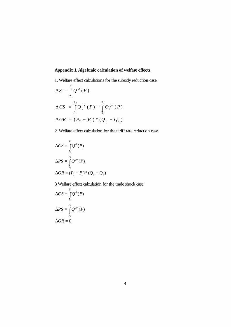
4
Appendix 1. Algebraic calculation of welfare effects 1. Welfare effect calculations for the subsidy reduction case.
)(*)(
)()(
)(
12
12
2
1
2
1
2
ca
p
p
prp
p
pr
p
p
d
QQPPGR
PQPQCS
PQSi
−−=∆
−=∆
=∆
∫∫
∫
2. Welfare effect calculation for the tariff rate reduction case
)(*)(
)(
)(
12
2
1
2
cd
p
p
pr
p
p
d
QQPPGR
PQPS
PQCSi
−−=∆
=∆
=∆
∫
∫
3 Welfare effect calculation for the trade shock case
0
)(
)(
2
1
2
=∆
=∆
=∆
∫
∫
GR
PQPS
PQCS
p
p
pr
p
p
di

5
Appendix 2. Results of Hausman test for simultaneity between production variables and price variables, demand variables and price variables, livestock_number variable and price variables Pr Milk Variables Entered/Removed(b)
Model Variables Entered
Variables
Removed Method
1 pRE_p_mILK, rES_p_MILk(a) . Enter
a All requested variables entered. b Dependent Variable: LnPrMilk Model Summary(b)
Model R R Square Adjusted R
Square Std. Error of the Estimate
1 1,000(a) 1,000 1,000 ,000000000 a Predictors: (Constant), pRE_p_mILK, rES_p_MILk b Dependent Variable: LnPrMilk Coefficients(a)
Unstandardized Coefficients
Standardized Coefficients
Model B Std. Error Beta t Sig. (Constant) 6,908 ,000 . . Res_p_MILk 1,000 ,000 ,788 . .
1
Pre_p_mILK 1,000 ,000 ,616 . . a Dependent Variable: LnPrMilk
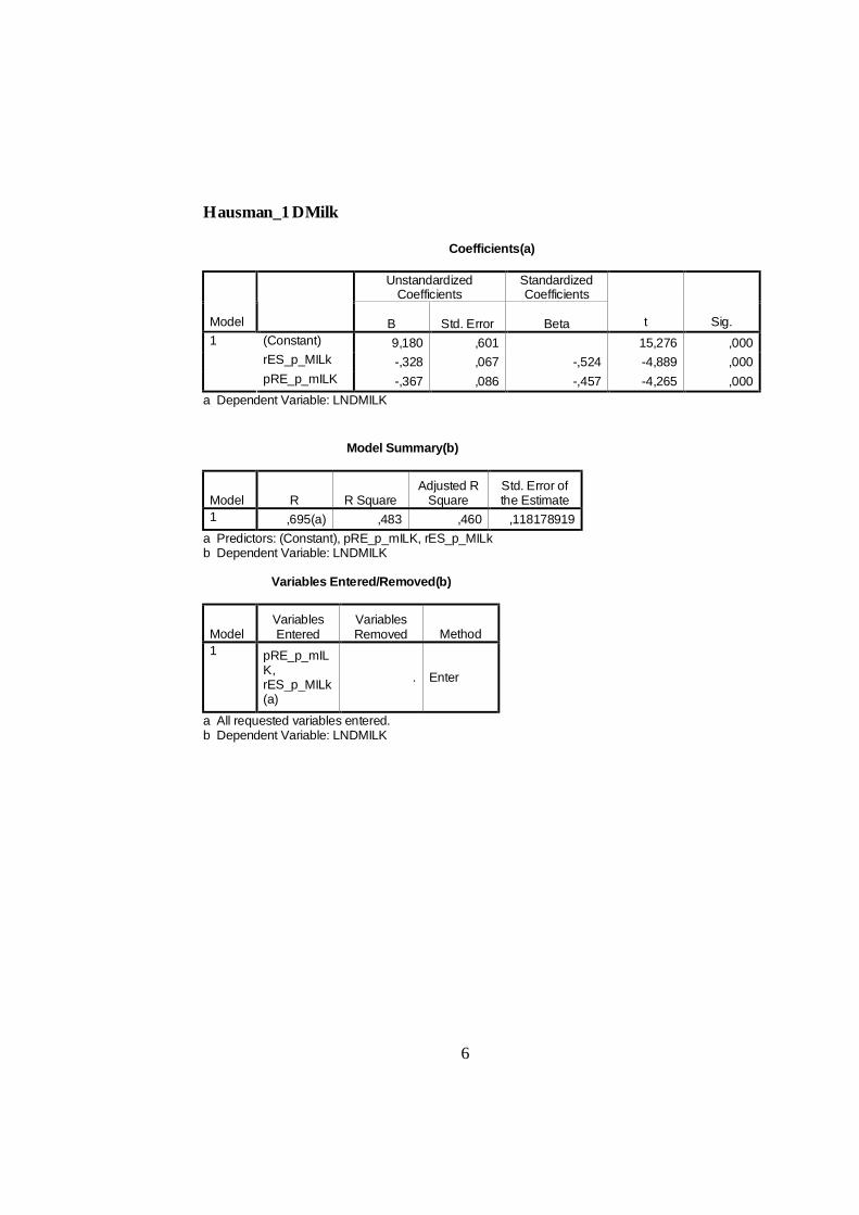
6
Hausman_1 DMilk Coefficients(a)
Unstandardized Coefficients
Standardized Coefficients
Model B Std. Error Beta t Sig. (Constant) 9,180 ,601 15,276 ,000 rES_p_MILk -,328 ,067 -,524 -4,889 ,000
1
pRE_p_mILK -,367 ,086 -,457 -4,265 ,000 a Dependent Variable: LNDMILK Model Summary(b)
Model R R Square Adjusted R
Square Std. Error of the Estimate
1 ,695(a) ,483 ,460 ,118178919 a Predictors: (Constant), pRE_p_mILK, rES_p_MILk b Dependent Variable: LNDMILK Variables Entered/Removed(b)
Model Variables Entered
Variables Removed Method
1 pRE_p_mILK, rES_p_MILk(a)
. Enter
a All requested variables entered. b Dependent Variable: LNDMILK

7
HAusman 1 – Pr Beef Variables Entered/Removed(b)
Model Variables Entered
Variables Removed Method
1 rES_p_bEEF, pRE_p_bEEF(a)
. Enter
a All requested variables entered. b Dependent Variable: LnPrBEEF Model Summary(b)
Model R R Square Adjusted R
Square Std. Error of the Estimate
1 ,293(a) ,086 ,045 ,2496367 a Predictors: (Constant), rES_p_bEEF, pRE_p_bEEF b Dependent Variable: LnPrBEEF Coefficients(a)
Unstandardized Coefficients
Standardized Coefficients
Model B Std. Error Beta t Sig. (Constant) 13,679 1,634 8,374 ,000 pRE_p_bEEF -,176 ,196 -,128 -,899 ,373
1
rES_p_bEEF -1,167 ,632 -,263 -1,845 ,072 a Dependent Variable: LnPrBEEF

8
Hausman_1 DBeef Variables Entered/Removed(b)
Model Variables Entered
Variables Removed Method
1 res_p_beef pre_p_beef . Enter
a All requested variables entered. b Dependent Variable: LnDBEFF Model Summary(b)
Model R R Square Adjusted R
Square Std. Error of the Estimate
1 ,211(a) ,044 ,002 ,2764922 a Predictors: (Constant), rES_p_bEEF, pRE_p_bEEF b Dependent Variable: LnDBEFF Coefficients(a)
Unstandardized Coefficients
Standardized Coefficients
Model B Std. Error Beta t Sig. (Constant) 12,540 1,809 6,931 ,000 Pre_p_beef -,041 ,217 -,028 -,189 ,851
1
Res_p_beef -1,004 ,700 -,209 -1,433 ,159 a Dependent Variable: LnDBEFF

9
Variables Entered/Removed(b)
Model Variables Entered
Variables
Removed Method
1
Res_p_milk, Pre_p_milk, Res_p_beef, Pre_p_beefF(a)
. Enter
a All requested variables entered. b Dependent Variable: LNSTOCK Model Summary(b)
Model R R Square Adjusted R
Square Std. Error of the Estimate
1 ,900(a) ,809 ,792 ,135662617 a Predictors: (Constant), rES_p_MILk, pRE_p_mILK, rES_p_bEEF, pRE_p_bEEF b Dependent Variable: LNSTOCK Coefficients(a)
Unstandardized Coefficients
Standardized Coefficients
Model B Std. Error Beta t Sig. (Constant) -3,437 1,037 -3,313 ,002 Pre_p_bEEF 1,413 ,108 ,885 13,069 ,000 Res_p_bEEF ,291 ,347 ,056 ,839 ,406 Pre_p_mILK ,023 ,100 ,016 ,232 ,818
1
Res_p_MILk -,165 ,078 -,142 -2,116 ,040 a Dependent Variable: LNSTOCK

10
Hausman_1 Ddairy Variables Entered/Removed(b)
Model Variables Entered
Variables Removed Method
1 res_dairy, pre_dairy(a) . Enter
a All requested variables entered. b Dependent Variable: lnD_dairy Model Summary(b)
Model R R Square Adjusted R
Square Std. Error of the Estimate
1 ,228(a) ,052 ,009 ,12335013 a Predictors: (Constant), res_dairy, pre_dairy b Dependent Variable: lnD_dairy Coefficients(a)
Unstandardized Coefficients
Standardized Coefficients
Model B Std. Error Beta t Sig. (Constant) 16,000 2,747 5,825 ,000 pre_dairy -,421 ,275 -,224 -1,529 ,133
1
res_dairy ,208 ,844 ,036 ,246 ,807 a Dependent Variable: lnD_dairy

11
Hausman 1 – Pr DAiry Variables Entered/Removed(b)
Model Variables Entered
Variables Removed Method
1 res_dairy, pre_dairy(a) . Enter
a All requested variables entered. b Dependent Variable: LnDprocmilk Model Summary(b)
Model R R Square Adjusted R
Square Std. Error of the Estimate
1 ,238(a) ,056 ,015 ,125146608 a Predictors: (Constant), res_dairy, pre_dairy b Dependent Variable: LnDprocmilk Coefficients(a)
Unstandardized Coefficients
Standardized Coefficients
Model B Std. Error Beta t Sig. (Constant) 16,423 2,777 5,914 ,000 pre_dairy -,457 ,278 -,238 -1,640 ,108
1
res_dairy ,027 ,848 ,005 ,032 ,975 a Dependent Variable: LnDprocmilk

12
Appendix 3. Output of Hausman test for simultaneity between Production variables and demand variables LnDProcMilk Coefficients(a)
Unstandardized Coefficients
Standardized Coefficients
Model B Std. Error Beta t Sig. (Constant) 16,677 3,042 5,482 ,000 Pre_dairy -,603 ,697 -,314 -,865 ,392 Res_dairy ,960 ,366 ,164 2,622 ,013 Pre_d_Milk -,323 ,439 -,311 -,736 ,466 Res_d_Milk -,258 ,127 -,216 -2,037 ,049 Pre_Pr_MILK ,274 ,185 ,435 1,482 ,147 Res_Pr_MILK ,118 ,052 ,241 2,260 ,030 Pre_PR_BEEF -,441 ,202 -,598 -2,185 ,035 Pr_dBeef ,404 ,154 ,555 2,621 ,013
1
Res_D_BEEF -,094 ,056 -,161 -1,694 ,098 a Dependent Variable: ANOVA(b)
Model Sum of
SquaRes df Mean Square F Sig. RegRession ,649 9 ,072 28,110 ,000(a) Residual ,098 38 ,003
1
Total ,747 47 a Predictors: (Constant), Res_D_BEEF, Pr_dBeef, Pre_dairy, Res_dairy, Pre_Pr_MILK, Res_d_Milk, Res_Pr_MILK, Pre_PR_BEEF, Pre_d_Milk b Dependent Variable: LnDProcMilk Model Summary(b)
Model R R Square Adjusted R
Square Std. Error of the Estimate
1 ,932(a) ,869 ,838 ,050664529 a Predictors: (Constant), Res_D_BEEF, Pr_dBeef, Pre_dairy, Res_dairy, Pre_Pr_MILK, Res_d_Milk, Res_Pr_MILK, Pre_PR_BEEF, Pre_d_Milk b Dependent Variable: LnDProcMilk Variables Entered/Removed(b)
Model Variables Entered
Variable
s Re Method
13
moved
1 Res_D_BEEF, Pr_dBeef, Pre_dairy, Res_dairy, Pre_Pr_MILK, Res_d_Milk, Res_Pr_MILK, Pre_PR_BEEF, Pre_d_Milk(a)
. Enter
a All requested variables entered. b Dependent Variable: LnDProcMilk
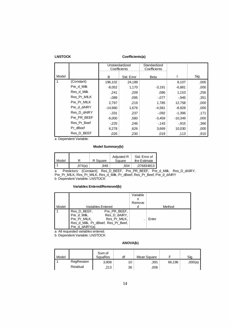
14
LNSTOCK Coefficients(a)
Unstandardized Coefficients
Standardized Coefficients
Model B Std. Error Beta t Sig. (Constant) 196,102 24,189 8,107 ,000 Pre_d_Milk -8,052 1,170 -3,191 -6,881 ,000 Res_d_Milk ,241 ,209 ,086 1,153 ,256 Res_Pr_MILK -,089 ,095 -,077 -,945 ,351 Pre_Pr_MILK 2,797 ,219 1,785 12,758 ,000 Pre_d_dAIRY -14,960 1,676 -4,581 -8,928 ,000 Res_D_dAIRY -,331 ,237 -,092 -1,396 ,171 Pre_PR_BEEF -6,000 ,580 -3,459 -10,349 ,000 Res_Pr_Beef -,225 ,246 -,143 -,915 ,366 Pr_dBeef 6,278 ,626 3,669 10,030 ,000
1
Res_D_BEEF ,026 ,230 ,019 ,113 ,910 a Dependent Variable: Model Summary(b)
Model R R Square Adjusted R
Square Std. Error of the Estimate
1 ,974(a) ,948 ,934 ,076834813 a Predictors: (Constant), Res_D_BEEF, Pre_PR_BEEF, Pre_d_Milk, Res_D_dAIRY, Pre_Pr_MILK, Res_Pr_MILK, Res_d_Milk, Pr_dBeef, Res_Pr_Beef, Pre_d_dAIRY b Dependent Variable: LNSTOCK Variables Entered/Removed(b)
Model Variables Entered
Variables
Removed Method
1 Res_D_BEEF, Pre_PR_BEEF, Pre_d_Milk, Res_D_dAIRY, Pre_Pr_MILK, Res_Pr_MILK, Res_d_Milk, Pr_dBeef, Res_Pr_Beef, Pre_d_dAIRY(a)
. Enter
a All requested variables entered. b Dependent Variable: LNSTOCK ANOVA(b)
Model Sum of
SquaRes df Mean Square F Sig. RegRession 3,908 10 ,391 66,196 ,000(a) 1 Residual ,213 36 ,006

15
Total 4,120 46 a Predictors: (Constant), Res_D_BEEF, Pre_PR_BEEF, Pre_d_Milk, Res_D_dAIRY, Pre_Pr_MILK, Res_Pr_MILK, Res_d_Milk, Pr_dBeef, Res_Pr_Beef, Pre_d_dAIRY b Dependent Variable: LNSTOCK

16
Coefficientsa
32,968 29,484 1,118 ,271-,572 1,835 -,235 -,312 ,757,509 ,477 ,068 1,067 ,293,422 ,658 ,503 ,642 ,525
-,076 ,070 -,123 -1,085 ,286-,914 ,861 -,983 -1,062 ,296,870 ,717 ,948 1,214 ,233,210 ,076 ,284 2,762 ,009
-,155 ,209 -,081 -,744 ,462-2,161 1,587 -1,233 -1,361 ,182-,056 ,091 -,102 -,612 ,544,477 ,258 ,173 1,850 ,073
(Constant)pre_dairyres_dairypRE_pr_MILKrES_pr_MILKpRE_PR_BBEFpR_dbEEFrES_D_BEEFres_D_dAIRYpRE_d_dAIRYPRE_STOCKrES_STOCK
Model1
B Std. Error
UnstandardizedCoefficients
Beta
StandardizedCoefficients
t Sig.
Dependent Variable: LNDMILKa.
ANOVA(b)
Model Sum of
SquaRes df Mean Square F Sig. RegRession 1,064 11 ,097 27,951 ,000(a) Residual ,121 35 ,003
1
Total 1,186 46 a Predictors: (Constant), Res_STOCK, Pre_PR_BEEF, PRE_STOCK, Res_dairy, Res_D_BEEF, Pre_Pr_MILK, Res_D_dAIRY, Res_Pr_MILK, Pre_d_dAIRY, Pre_dairy, Pr_dBeef b Dependent Variable: LNDMILK Model Summary(b)
Model R R Square Adjusted R
Square Std. Error of the Estimate
1 ,948(a) ,898 ,866 ,058838066 a Predictors: (Constant), Res_STOCK, Pre_PR_BEEF, PRE_STOCK, Res_dairy, Res_D_BEEF, Pre_Pr_MILK, Res_D_dAIRY, Res_Pr_MILK, Pre_d_dAIRY, Pre_dairy, Pr_dBeef b Dependent Variable: LNDMILK Variables Entered/Removed(b)
Model Variables Entered Variables Removed Method

17
1 Res_STOCK, Pre_PR_BEEF, PRE_STOCK, Res_dairy, Res_D_BEEF, Pre_Pr_MILK, Res_D_dAIRY, Res_Pr_MILK, Pre_d_dAIRY, Pre_dairy, Pr_dBeef(a)
. Enter
a All requested variables entered. b Dependent Variable: LNDMILK

18
LnPrMilk Variables Entered/Removed(b)
Model Variables Entered Variables Removed Method
1 Res_d_Milk, Pre_PR_BEEF, PRE_STOCK, Res_dairy, Res_STOCK, Pre_d_dAIRY, Res_D_BEEF, Res_D_dAIRY, Pre_dairy, Pr_dBeef, Pre_d_Milk(a)
. Enter
a All requested variables entered. b Dependent Variable: Model Summary(b)
Model R R Square Adjusted R
Square Std. Error of the Estimate
1 ,925(a) ,856 ,810 ,138971279 a Predictors: (Constant), Res_d_Milk, Pre_PR_BEEF, PRE_STOCK, Res_dairy, Res_STOCK, Pre_d_dAIRY, Res_D_BEEF, Res_D_dAIRY, Pre_dairy, Pr_dBeef, Pre_d_Milk b Dependent Variable: LnPrMilk Coefficients(a)
Unstandardized Coefficients
Standardized Coefficients
Model B Std. Error Beta t Sig. (Constant) -56,648 28,002 -2,023 ,051 Pre_dairy 1,816 1,802 ,376 1,008 ,321 Res_dairy -1,013 1,132 -,068 -,895 ,377 Pre_PR_BEEF 1,590 ,826 ,860 1,924 ,063 Pr_dBeef -1,507 ,956 -,826 -1,576 ,124 Res_D_BEEF -,484 ,181 -,329 -2,672 ,011 Res_D_dAIRY ,273 ,495 ,071 ,552 ,584 Pre_d_dAIRY 3,614 2,293 1,038 1,576 ,124 PRE_STOCK ,077 ,261 ,071 ,297 ,768 Res_STOCK -1,592 ,579 -,291 -2,752 ,009 Pre_d_Milk 1,222 2,183 ,454 ,560 ,579
1
Res_d_Milk -,426 ,393 -,142 -1,085 ,286 a Dependent Variable: LnPrMilk ANOVA(b)
Model Sum of
SquaRes df Mean Square F Sig. RegRession 4,008 11 ,364 18,866 ,000(a) Residual ,676 35 ,019
1
Total 4,684 46

19
a Predictors: (Constant), Res_d_Milk, Pre_PR_BEEF, PRE_STOCK, Res_dairy, Res_STOCK, Pre_d_dAIRY, Res_D_BEEF, Res_D_dAIRY, Pre_dairy, Pr_dBeef, Pre_d_Milk b Dependent Variable: LnPrMilk
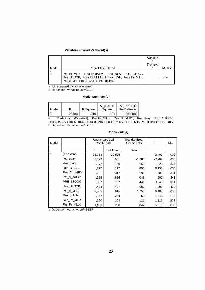
20
Variables Entered/Removed(b)
Model Variables Entered
Variables
Removed Method
1 Pre_Pr_MILK, Res_D_dAIRY, Res_dairy, PRE_STOCK, Res_STOCK, Res_D_BEEF, Res_d_Milk, Res_Pr_MILK, Pre_d_Milk, Pre_d_dAIRY, Pre_dairy(a)
. Enter
a All requested variables entered. b Dependent Variable: LnPrBEEF Model Summary(b)
Model R R Square Adjusted R
Square Std. Error of the Estimate
1 ,954(a) ,910 ,881 ,0885888 a Predictors: (Constant), Pre_Pr_MILK, Res_D_dAIRY, Res_dairy, PRE_STOCK, Res_STOCK, Res_D_BEEF, Res_d_Milk, Res_Pr_MILK, Pre_d_Milk, Pre_d_dAIRY, Pre_dairy b Dependent Variable: LnPrBEEF Coefficients(a)
Model Unstandardized
Coefficients Standardized Coefficients t Sig.
B Std. Error Beta 1 (Constant) 35,788 10,505 3,407 ,002 Pre_dairy -7,329 ,951 -1,883 -7,707 ,000 Res_dairy -,672 ,730 -,056 -,920 ,364 Res_D_BEEF ,777 ,127 ,655 6,138 ,000 Res_D_dAIRY -,281 ,317 -,091 -,888 ,381 Pre_d_dAIRY ,135 ,666 ,048 ,202 ,841 PRE_STOCK ,387 ,127 ,441 3,040 ,004 Res_STOCK -,403 ,407 -,091 -,991 ,329 Pre_d_Milk 3,805 ,615 1,755 6,182 ,000 Res_d_Milk ,367 ,254 ,152 1,442 ,158 Res_Pr_MILK ,120 ,108 ,121 1,115 ,273 Pre_Pr_MILK 1,403 ,280 1,042 5,016 ,000
a Dependent Variable: LnPrBEEF
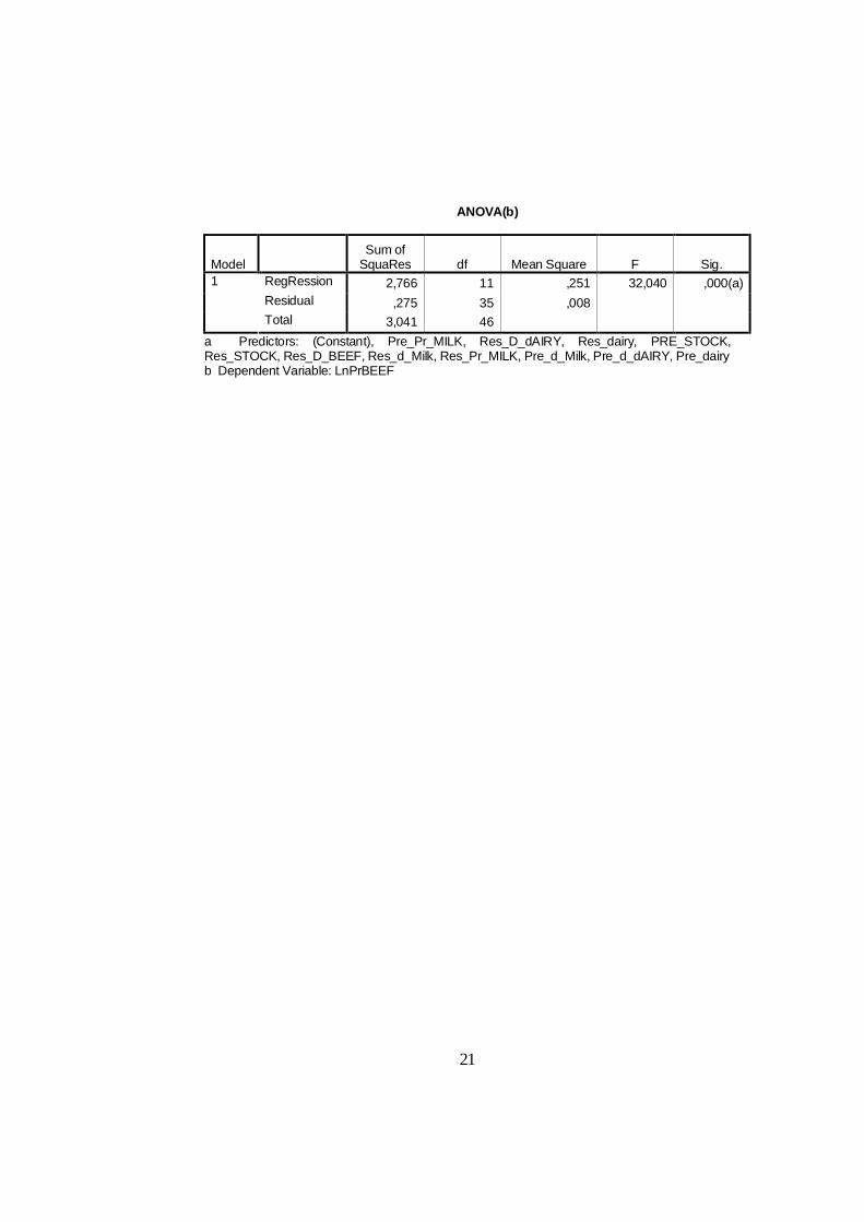
21
ANOVA(b)
Model Sum of
SquaRes df Mean Square F Sig. RegRession 2,766 11 ,251 32,040 ,000(a) Residual ,275 35 ,008
1
Total 3,041 46 a Predictors: (Constant), Pre_Pr_MILK, Res_D_dAIRY, Res_dairy, PRE_STOCK, Res_STOCK, Res_D_BEEF, Res_d_Milk, Res_Pr_MILK, Pre_d_Milk, Pre_d_dAIRY, Pre_dairy b Dependent Variable: LnPrBEEF

22
Coefficients(a)
Model Unstandardized
Coefficients Standardized Coefficients t Sig.
B Std. Error Beta 1 (Constant) -,146 16,609 -,009 ,993 Pre_dairy -6,878 1,500 -1,632 -4,587 ,000 Res_dairy ,372 1,151 ,029 ,323 ,749 Res_D_dAIRY -1,102 ,449 -,330 -2,452 ,019 Pre_d_dAIRY 2,598 1,053 ,855 2,467 ,019 PRE_STOCK ,467 ,201 ,492 2,321 ,026 Res_STOCK -1,818 ,530 -,381 -3,431 ,002 Pre_d_Milk 5,043 ,971 2,149 5,196 ,000 Res_d_Milk ,854 ,365 ,326 2,343 ,025 Res_Pr_MILK -,349 ,155 -,325 -2,249 ,031 Pre_Pr_MILK ,933 ,441 ,640 2,118 ,041
a Dependent Variable: LnDBEFF ANOVA(b)
Model Sum of
SquaRes df Mean Square F Sig. RegRession 2,859 10 ,286 14,572 ,000(a) Residual ,706 36 ,020
1
Total 3,565 46 a Predictors: (Constant), Pre_Pr_MILK, Res_D_dAIRY, Res_dairy, PRE_STOCK, Res_STOCK, Res_d_Milk, Res_Pr_MILK, Pre_d_Milk, Pre_d_dAIRY, Pre_dairy b Dependent Variable: LnDBEFF Model Summary(b)
Model R R Square Adjusted R
Square Std. Error of the Estimate
1 ,895(a) ,802 ,747 ,1400603 a Predictors: (Constant), Pre_Pr_MILK, Res_D_dAIRY, Res_dairy, PRE_STOCK, Res_STOCK, Res_d_Milk, Res_Pr_MILK, Pre_d_Milk, Pre_d_dAIRY, Pre_dairy b Dependent Variable: LnDBEFF Variables Entered/Removed(b)
Model Variables Entered Variables Removed Method
1 Pre_Pr_MILK, Res_D_dAIRY, Res_dairy, PRE_STOCK, Res_STOCK, Res_d_Milk, Res_Pr_MILK, Pre_d_Milk, Pre_d_dAIRY, Pre_dairy(a)
. Enter

23
a All requested variables entered. b Dependent Variable: LnDBEFF

24
Coefficients(a)
Unstandardized Coefficients
Standardized Coefficients
Model B Std. Error Beta t Sig. (Constant) 13,985 2,835 4,934 ,000 Pre_dairy ,074 ,585 ,040 ,127 ,900 Res_dairy 1,184 ,401 ,206 2,955 ,005 PRE_STOCK ,019 ,078 ,046 ,248 ,806 Res_STOCK -,313 ,200 -,147 -1,564 ,126 Pre_d_Milk -,674 ,288 -,645 -2,339 ,025 Res_d_Milk -,315 ,132 -,271 -2,395 ,022 Res_Pr_MILK ,114 ,057 ,238 1,991 ,054
1
Pre_Pr_MILK ,098 ,161 ,152 ,613 ,544 a Dependent Variable: lnD_dairy ANOVA(b)
Model Sum of
SquaRes df Mean Square F Sig. RegRession ,592 8 ,074 24,659 ,000(a) Residual ,114 38 ,003
1
Total ,706 46 a Predictors: (Constant), Pre_Pr_MILK, Res_Pr_MILK, PRE_STOCK, Res_dairy, Res_STOCK, Res_d_Milk, Pre_d_Milk, Pre_dairy b Dependent Variable: lnD_dairy Model Summary(b)
Model R R Square Adjusted R
Square Std. Error of the Estimate
1 ,916(a) ,838 ,804 ,05478403 a Predictors: (Constant), Pre_Pr_MILK, Res_Pr_MILK, PRE_STOCK, Res_dairy, Res_STOCK, Res_d_Milk, Pre_d_Milk, Pre_dairy b Dependent Variable: lnD_dairy Variables Entered/Removed(b)
Model Variables Entered Variables Removed Method
1 Pre_Pr_MILK, Res_Pr_MILK, PRE_STOCK, Res_dairy, Res_STOCK, Res_d_Milk, Pre_d_Milk, Pre_dairy(a)
. Enter
a All requested variables entered. b Dependent Variable: lnD_dairy

25

26
Appendix 4. A. Estimation output of beef production function: regression on significant variables Model Description Type of Variable
LnPrBEEF dependent LnStock_lag_1
predictor
LNPBEEF
predictor
LNPMILK
predictor
LNPLABOR
predictor
LnInc
instrumental
LnPother_all
instrumental
LnPother_crop
instrumental
LnPOther_animal
instrumental
LnDMilk_lag_1
instrumental
ln_Price_ratio
instrumental
LnPdairy
instrumental
LnStock_lag_2
instrumental
LnPbeef_lag_1
instrumental
LnPMilk_lag_1
instrumental
LnPFeed_lag_1
instrumental
LnPLabor_lag_1
instrumental
LnPBeef_lag_2
instrumental
LnPFeed_lag_2
instrumental
Equation 1
LnPMilk_lag_2
instrumental

27
LnPLabor_lag_2
instrumental
MOD_37 Model Summary
Multiple R ,755
R Square
,570
Adjusted R Square
,530
Equation 1
Std. Error of the Estimate
,186
Coefficients
Unstandardized Coefficients
B
Std. Error Beta
(Constant) 19,793 1,470 LnStock_lag_1
-1,448 ,498 -1,640
LNPBEEF
,695 ,464 ,530
Equation 1
LNPMILK
-,827 ,127 -1,053
LNPLABOR
,814 ,209 1,301 3,889
F=14,243
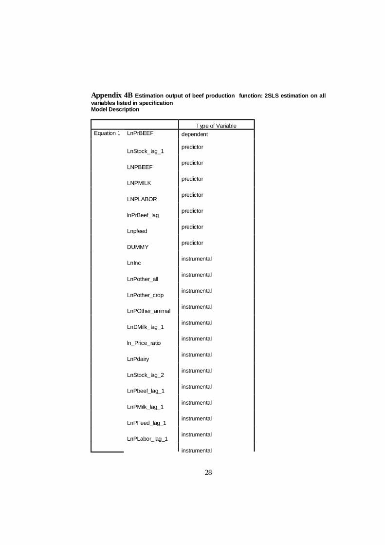
28
Appendix 4B Estimation output of beef production function: 2SLS estimation on all variables listed in specification Model Description Type of Variable
LnPrBEEF dependent LnStock_lag_1
predictor
LNPBEEF
predictor
LNPMILK
predictor
LNPLABOR
predictor
lnPrBeef_lag
predictor
Lnpfeed
predictor
DUMMY
predictor
LnInc
instrumental
LnPother_all
instrumental
LnPother_crop
instrumental
LnPOther_animal
instrumental
LnDMilk_lag_1
instrumental
ln_Price_ratio
instrumental
LnPdairy
instrumental
LnStock_lag_2
instrumental
LnPbeef_lag_1
instrumental
LnPMilk_lag_1
instrumental
LnPFeed_lag_1
instrumental
LnPLabor_lag_1
instrumental
Equation 1
instrumental

29
LnPBeef_lag_2
LnPFeed_lag_2
instrumental
LnPMilk_lag_2
instrumental
LnPLabor_lag_2
instrumental
MOD_40 Model Summary
Multiple R ,744 R Square
,554
Adjusted R Square
,474
Equation 1
Std. Error of the Estimate
,199
Coefficients
Unstandardized Coefficients
B
Std. Error Beta
(Constant) 20,436 6,185 LnStock_lag_1
-1,561 ,689 -1,727
LNPBEEF
,774 ,620 ,574
LNPMILK
-,804 ,288 -1,007
LNPLABOR
,847 ,271 1,311
lnPrBeef_lag
-,037 ,329 -,035
Equation 1
Lnpfeed
-,042 ,200 -,038
DUMMY
,047 ,157 ,087 ,302
F=6,927

30
Appendix 4C Estimation output of beef production function: OLS method Coefficients(a)
Unstandardized Coefficients Standardized Coefficients
Model B Std. Error
Beta
(Constant) 23,207 5,168 lnPrBeef_lag
-,113 ,184 -,108
LNPBEEF
-1,108 ,490 -,823
LNPMILK
-,668 ,200 -,837
Lnpfeed
-,374 ,332 -,343
LNPLABOR
,668 ,323 1,034
LnStock_lag_1
-,460 ,561 -,509
LnPother_all
,170 1,206 ,067
LnPother_crop
,303 ,591 ,224
1
LnPOther_animal
,931 ,583 ,671
DUMMY
-,041 ,105 -,076 -,392
a Dependent Variable: LnPrBEEF F=6,929 Model Summary(b)
Model R R Square Adjusted R
Square Std. Error of the Estimate
1 ,811(a) ,658 ,563 ,1691924 a Predictors: (Constant), DUMMY, LnStock_lag_1, LnPother_all, lnPrBeef_lag, LnPother_crop, LNPMILK, Lnpfeed, LNPBEEF, LnPOther_animal, LNPLABOR b Dependent Variable: LnPrBEEF

31
Appendix 5C Estimation output of dairy production function: OLS method Dairy production variable: OLS maethod Variables Entered/Removed(b)
Model Variables Entered
Variables Removed Method
1 LNPLABOR, ln_Price_ratio, LnPOther_animal, LnPother_crop, LNPMILK, LnPdairy, LNPBEEF, LnPother_all(a)
. Enter
a All requested variables entered. b Dependent Variable: LnDprocmilk Coefficients(a)
Unstandardized Coefficients
Standardized Coefficients
Model B Std. Error
Beta t Sig.
(Constant) 2,349 3,199 ,734 ,467 LNPMILK
,161 ,048 ,416 3,331 ,002
LnPdairy
,968 ,356 ,530 2,721 ,010
LnPother_all
-,038 ,285 -,031 -,132 ,896
LnPother_crop
,088 ,147 ,131 ,598 ,553
LnPOther_animal
-,172 ,183 -,256 -,943 ,351
ln_Price_ratio
1,417 ,381 ,470 3,724 ,001
1
LNPBEEF
-,216 ,132 -,334 -1,638 ,109

32
LNPLABOR
-,100 ,059 -,324 -1,689 ,099
a Dependent Variable: LnDprocmilk Model Summary
Model R R Square Adjusted R
Square Std. Error of the Estimate
1 ,926(a) ,858 ,829 ,052198339 a Predictors: (Constant), LNPLABOR, ln_Price_ratio, LnPOther_animal, LnPother_crop, LNPMILK, LnPdairy, LNPBEEF, LnPother_all
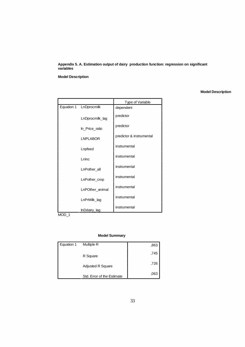
33
Appendix 5. A. Estimation output of dairy production function: regression on significant variables Model Description Model Description Type of Variable
LnDprocmilk dependent LnDprocmilk_lag
predictor
ln_Price_ratio
predictor
LNPLABOR
predictor & instrumental
Lnpfeed
instrumental
LnInc
instrumental
LnPother_all
instrumental
LnPother_crop
instrumental
LnPOther_animal
instrumental
LnPrMilk_lag
instrumental
Equation 1
lnDdairy_lag
instrumental
MOD_1 Model Summary
Multiple R ,863 R Square
,745
Adjusted R Square
,726
Equation 1
Std. Error of the Estimate
,063

34
Coefficients
Unstandardized Coefficients
B
Std. Error Beta t Sig.
(Constant) 7,573 1,216 6,229 ,000
LnDprocmilk_lag
,164 ,133 ,164 1,235 ,224
Equation 1
ln_Price_ratio
2,162 ,422 ,727 5,119 ,000
LNPLABOR
-,045 ,024 -,144 -1,902 ,064
F=40,281

35
Appendix 5B Estimation output of dairy production function: 2SLS estimation on all variables listed in specification Model Description Type of Variable
LnDprocmilk dependent ln_Price_ratio
predictor
lnDdairy_lag
predictor
LNPLABOR
predictor & instrumental
LnPother_all
predictor & instrumental
LnPother_crop
predictor & instrumental
LnPOther_animal
predictor & instrumental
Lnpfeed
instrumental
LnInc
instrumental
Equation 1
LnPrBEEF
instrumental
MOD_22 Model Summary
Multiple R ,807 R Square
,652
Adjusted R Square
,598
Equation 1
Std. Error of the Estimate
,088
Coefficients
Unstandardized Coefficients
B
Std. Error Beta
Equation 1

36
(Constant) 1,566 5,521 ln_Price_ratio
1,160 1,150 ,390
lnDdairy_lag
,903 ,624 ,901
LNPLABOR
-,070 ,040 -,225
LnPother_all
,752 ,795 ,615
LnPother_crop
-,526 ,475 -,782
LnPOther_animal
-,512 ,420 -,755 -1,218
F=12,73
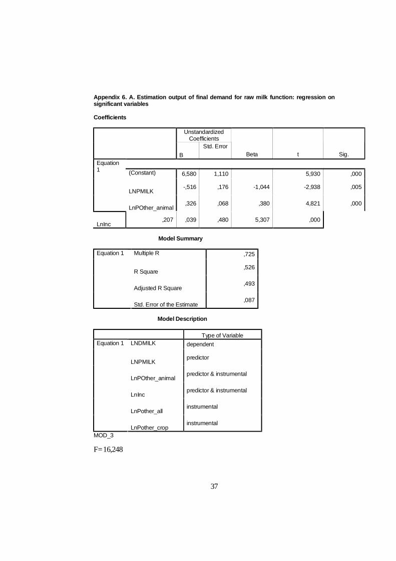
37
Appendix 6. A. Estimation output of final demand for raw milk function: regression on significant variables Coefficients
Unstandardized Coefficients
B
Std. Error Beta t Sig.
(Constant) 6,580 1,110 5,930 ,000 LNPMILK
-,516 ,176 -1,044 -2,938 ,005
Equation 1
LnPOther_animal
,326 ,068 ,380 4,821 ,000
LnInc
,207 ,039 ,480 5,307 ,000
Model Summary
Multiple R ,725
R Square
,526
Adjusted R Square
,493
Equation 1
Std. Error of the Estimate
,087
Model Description Type of Variable
LNDMILK dependent
LNPMILK
predictor
LnPOther_animal
predictor & instrumental
LnInc
predictor & instrumental
LnPother_all
instrumental
Equation 1
LnPother_crop
instrumental
MOD_3 F=16,248

38
Appendix 6C Estimation output of final demand for raw milk function: OLS method Variables Entered/Removed(b)
Model Variables Entered Variables Removed Method
1 LnPdairy, LnPother_all, LNPMILK, LnInc, LnPother_crop, LNPBEEF, LnPOther_animal(a)
. Enter
a All requested variables entered. b Dependent Variable: LNDMILK ANOVA(b)
Model Sum of Squares F Sig.
1 Regression 1,027 30,913 ,000(a) Residual ,190 Total 1,216
a Predictors: (Constant), LnPdairy, LnPother_all, LNPMILK, LnInc, LnPother_crop, LNPBEEF, LnPOther_animal b Dependent Variable: LNDMILK Model Summary
Model R R Square Adjusted R
Square Std. Error of the Estimate
1 ,919(a) ,844 ,817 ,068878111 a Predictors: (Constant), LnPdairy, LnPother_all, LNPMILK, LnInc, LnPother_crop, LNPBEEF, LnPOther_animal Coefficients(a)
Unstandardized Coefficients
Standardized Coefficients
Model B Std. Error
Beta t Sig.
(Constant) 9,02
2 3,326 2,712 ,010
LnInc
,259 ,060 ,602 4,305 ,000
LnPother_all
-,022 ,381 -,014 -,058 ,954
1
-
,219 ,200 -,256 -1,095 ,280

39
LnPother_crop
LnPOther_animal
,459 ,211 ,534 2,174 ,036
LNPBEEF
-,273 ,161 -,331 -1,702 ,096
LNPMILK
-,349 ,033 -,706
-10,50
9 ,000
LnPdairy
-,137 ,395 -,059 -,346 ,731
a Dependent Variable: LNDMILK

40
Appendix 6B Estimation output of final demand for raw milk function: 2SLS estimation on all variables listed in specification Coefficients
Unstandardized Coefficients
B
Std. Error Beta t Sig.
(Constant) 6,740 3,384 1,992 ,053
LNPMILK
-,176 ,355 -,356 -,496 ,623
LnPOther_animal
,393 ,159 ,458 2,473 ,018
LnInc
,280 ,122 ,649 2,299 ,027
VAR00025
,220 ,265 ,653 ,833 ,410
Equation 1
LnPdairy
-,411 ,717 -,176 -,574 ,569
LnDMilk_lag_1
,066 ,167 ,064 ,397 ,693
Model Summary
Multiple R ,895 R Square
,802
Adjusted R Square
,773
Equation 1
Std. Error of the Estimate
,085
F=27,619

41
Appendix 7. A. Estimation output of demand for dairy function: regression on significant variables Model Summary
Multiple R ,768 R Square
,590
Adjusted R Square
,571
Equation 1
Std. Error of the Estimate
,091
Model Description Type of Variable
lnD_dairy dependent LnPdairy
predictor
LNPMILK
predictor
Lnpfeed
instrumental
LNPLABOR
instrumental
LnInc
instrumental
LnPother_all
instrumental
LnPother_crop
instrumental
LnPOther_animal
instrumental
Equation 1
LnPrBEEF
instrumental
MOD_10 Coefficients
Unstandardized Coefficients
B
Std. Error Beta t Sig.
(Constant) 17,257 2,030 8,499 ,000
Equation 1
LnPdairy
-,847 ,211 -,473 -4,022 ,000

42
LNPMILK
,428 ,056 1,102 7,698 ,000
F=31,643
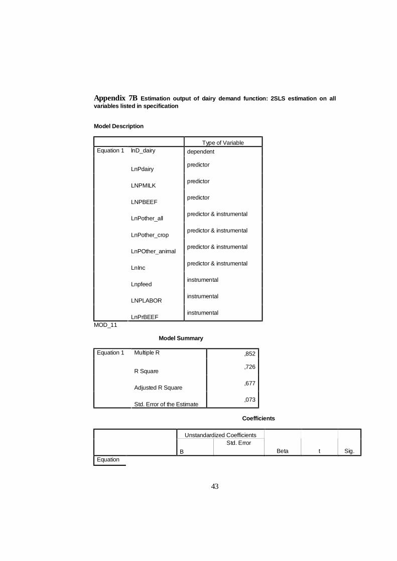
43
Appendix 7B Estimation output of dairy demand function: 2SLS estimation on all variables listed in specification Model Description Type of Variable
lnD_dairy dependent LnPdairy
predictor
LNPMILK
predictor
LNPBEEF
predictor
LnPother_all
predictor & instrumental
LnPother_crop
predictor & instrumental
LnPOther_animal
predictor & instrumental
LnInc
predictor & instrumental
Lnpfeed
instrumental
LNPLABOR
instrumental
Equation 1
LnPrBEEF
instrumental
MOD_11 Model Summary
Multiple R ,852
R Square
,726
Adjusted R Square
,677
Equation 1
Std. Error of the Estimate
,073
Coefficients
Unstandardized Coefficients
B
Std. Error Beta t Sig.
Equation

44
(Constant) 5,957 8,139 ,732 ,469 LnPdairy
,748 ,969 ,418 ,772 ,445
LNPMILK
,413 ,075 1,063 5,492 ,000
LNPBEEF
-,385 ,369 -,610 -1,043 ,303
LnPother_all
,364 ,528 ,306 ,688 ,495
LnPother_crop
-,158 ,355 -,237 -,446 ,658
1
LnPOther_animal
-,313 ,248 -,473 -1,261 ,215
LnInc
-,077 ,138 -,233 -,555 ,582
F=14.473

45
Appendix 6C Estimation output of dairy demand function: OLS method Variables Entered/Removed(b)
Model Variables Entered Variables Removed Method
1 LNPMILK, LnPother_all, LnPdairy, LnInc, lnDdairy_lag, LnPOther_animal, LNPBEEF, LnPother_crop(a)
. Enter
a All requested variables entered. b Dependent Variable: lnD_dairy Model Summary
Model R R Square Adjusted R
Square Std. Error of the Estimate
1 ,912(a) ,832 ,795 ,05559341 a Predictors: (Constant), LNPMILK, LnPother_all, LnPdairy, LnInc, lnDdairy_lag, LnPOther_animal, LNPBEEF, LnPother_crop Coefficients(a)
Unstandardized Coefficients Standardized Coefficients
Model B Std. Error
Beta t Sig.
(Constant) -2,731 2,925 -,934 ,357 lnDdairy_lag
,293 ,126 ,299 2,320 ,026
LnPdairy
1,423 ,327 ,783 4,352 ,000
LnInc
-,234 ,053 -,704 -4,419 ,000
LnPother_all
,233 ,362 ,196 ,643 ,524
LnPother_crop
-,026 ,198 -,038 -,130 ,897
LnPOther_animal
-,513 ,192 -,771 -2,669 ,011
1
LNPBEEF
-,076 ,132 -,119 -,579 ,566
,192 ,047 ,482 4,088 ,000

46
LNPMILK
a Dependent Variable: lnD_dairy F=22,279

47
Appendix 8. A. Estimation output of livestock number function: regression on significant variables Model Description Type of Variable
LNSTOCK dependent
LNPMILK
predictor
LNPBEEF
predictor
LnStock_lag_1
predictor
LnInc
instrumental
LnPother_all
instrumental
LnPother_crop
instrumental
LnPOther_animal
instrumental
LnDMilk_lag_1
instrumental
ln_Price_ratio
instrumental
Equation 1
LnPdairy
instrumental
MOD_16 Coefficients
Unstandardized Coefficients
B
Std. Error Beta t Sig.
(Constant) ,153(,626) ,311 ,492 LNPMILK
,039(,101) ,023 ,042 1,676
Equation 1
LNPBEEF
-,208(,016) ,083 -,136 -2,498
LnStock_lag_1
1,152(,000) ,053 1,121 21,613
Model Summary

48
Multiple R ,991 R Square
,982
Adjusted R Square
,981
Equation 1
Std. Error of the Estimate
,041
F=766,619

49
Appendix 8B Estimation output of livestock number function: 2SLS estimation on all variables listed in specification Model Description Type of Variable
LNSTOCK dependent LNPBEEF
predictor
LNPMILK
predictor
LnStock_lag_1
predictor
LNPLABOR
predictor & instrumental
Lnpfeed
predictor & instrumental
LnPOther_animal
predictor & instrumental
LnInc
instrumental
LnPother_all
instrumental
LnPother_crop
instrumental
LnPrMilk_lag
instrumental
Equation 1
lnDdairy_lag
instrumental
MOD_17 Model Summary
Multiple R ,990
R Square
,980
Adjusted R Square
,977
Equation 1
Std. Error of the Estimate
,045
Coefficients
Unstandardized Coefficients Std. Error Beta t Sig.
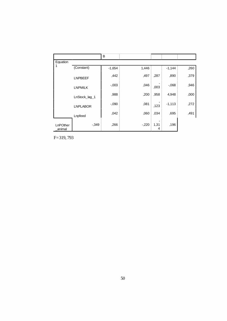
50
B
(Constant) -1,654 1,446 -1,144 ,260
LNPBEEF
,442 ,497 ,287 ,890 ,379
LNPMILK
-,003 ,046 -,003 -,068 ,946
LnStock_lag_1
,988 ,200 ,958 4,948 ,000
LNPLABOR
-,090 ,081 -,123 -1,113 ,272
Equation 1
Lnpfeed
,042 ,060 ,034 ,695 ,491
LnPOther_animal
-,349 ,266 -,220 -
1,314
,196
F=319, 793

51
Appendix 8C Estimation output of livestock number function: OLS method Variables Entered/Removed(b)
Model Variables Entered
Variables Removed Method
1
Lnpfeed, VAR00001, LNPBEEF, LNPMILK, LNPLABOR, LnStock_lag_1(a)
. Enter
a All requested variables entered. b Dependent Variable: LNSTOCK Model Summary
Model R R Square Adjusted R
Square Std. Error of the Estimate
1 ,995(a) ,990 ,988 ,031962898 a Predictors: (Constant), Lnpfeed, VAR00001, LNPBEEF, LNPMILK, LNPLABOR, LnStock_lag_1 Coefficients(a)
Unstandardized Coefficients
Standardized Coefficients
Model B Std. Error
Beta t Sig.
(Constant) ,531 ,329 1,614 ,114 LNPMILK
,007 ,019 ,008 ,366 ,716
LNPBEEF
,130 ,066 ,085 1,961 ,057
VAR00001
,051 ,014 ,081 3,500 ,001
LNPLABOR
,155 ,038 ,212 4,040 ,000
1
,733 ,080 ,713 9,151 ,000

52
LnStock_lag_1
Lnpfeed
-,053 ,028 -,042 -1,876 ,068
a Dependent Variable: LNSTOCK F=670,683

53

54
Appendix 10B Estimation output of milk production function: 2SLS estimation on all variables listed in specification Model Description Type of Variable
LnPrMilk_lag dependent LNPMILK
predictor
LnStock_lag_1
predictor
LnPdairy
predictor & instrumental
LNPBEEF
predictor
LNPLABOR
predictor
LnPother_all
predictor & instrumental
LnPother_crop
predictor & instrumental
LnPOther_animal
predictor & instrumental
Lnpfeed
predictor
DUMMY
predictor
LnInc
instrumental
LnDMilk_lag_1
instrumental
ln_Price_ratio
instrumental
LnStock_lag_2
instrumental
LnPbeef_lag_1
instrumental
LnPMilk_lag_1
instrumental
LnPFeed_lag_1
instrumental
LnPLabor_lag_1
instrumental
LnPBeef_lag_2
instrumental
Equation 1
instrumental

55
LnPFeed_lag_2
LnPMilk_lag_2
instrumental
LnPLabor_lag_2
instrumental
MOD_1 Coefficients
Unstandardized Coefficients
B
Std. Error Beta t Sig.
(Constant) 22,460 8,112 2,769 ,009 LNPMILK
,430 ,192 ,425 2,242 ,031
LnStock_lag_1
-1,431 ,539 -1,249 -2,655 ,012
LnPdairy
-1,164 ,878 -,242 -1,326 ,193
LNPBEEF
,632 ,657 ,370 ,963 ,342
LNPLABOR
,795 ,288 ,971 2,764 ,009
LnPother_all
,951 ,912 ,297 1,043 ,304
LnPother_crop
-,064 ,405 -,037 -,157 ,876
LnPOther_animal
,377 ,411 ,214 ,917 ,365
Lnpfeed
-,590 ,380 -,427 -1,550 ,130
Equation 1
DUMMY
-,199 ,091 -,289 -2,189 ,035
VAR00010 1,001 ,488 1,044 2,052 ,047 Model Summary
Multiple R ,953
R Square
,908
Adjusted R Square
,883
Equation 1
,111

56
Std. Error of the Estimate
F=35,624

57
Appendix 10.A. Estimation output of mil production function: regression on significant variables Model Description Type of Variable
LnPrMilk_lag dependent
LNPMILK
predictor
LnStock_lag_1
predictor
Lnpfeed
predictor
DUMMY
predictor
LnPother_all
predictor & instrumental
LnInc
instrumental
LnPother_crop
instrumental
LnPOther_animal
instrumental
LnDMilk_lag_1
instrumental
ln_Price_ratio
instrumental
LnPdairy
instrumental
LnStock_lag_2
instrumental
LnPbeef_lag_1
instrumental
LnPMilk_lag_1
instrumental
LnPFeed_lag_1
instrumental
LnPLabor_lag_1
instrumental
LnPBeef_lag_2
instrumental
LnPFeed_lag_2
instrumental
LnPMilk_lag_2
instrumental
Equation 1
instrumental

58
LnPLabor_lag_2 MOD_27 Model Summary
Multiple R ,930 R Square
,865
Adjusted R Square
,848
Equation 1
Std. Error of the Estimate
,125
Coefficients
Unstandardized Coefficients
B
Std. Error Beta t Sig.
(Constant) 11,425 1,543 7,404 ,000 LNPMILK
,512 ,136 ,506 3,766 ,001
LnStock_lag_1
-,348 ,124 -,304 -2,815 ,007
Lnpfeed
-,905 ,239 -,656 -3,790 ,000
Equation 1
DUMMY
-,354 ,091 -,514 -3,908 ,000
LnPother_all
1,583 ,402 ,494 3,934 ,000
F=33,278

59
Appendix 10C Estimation output of milk production function: OLS method Coefficients(a)
Unstandardized Coefficients
Standardized
Coefficients
Model B
Std. Error
Beta t Sig.
(Constant) -27,422 8,193 -3,347 ,002
LNPBEEF
,262 ,413 ,155 ,634 ,530
VAR00001
,146 ,097 ,214 1,510 ,139
LNPLABOR
-,717 ,294 -,886 -2,441 ,019
LnStock_lag_1
,553 ,485 ,488 1,140 ,262
Lnpfeed
,326 ,167 ,239 1,951 ,058
LnPrMilk_lag
1,189 ,142 1,203 8,389 ,000
1
LnPOther_animal
-1,138 ,370 -,655 -3,072 ,004
LnPdairy
2,551 ,981 ,538 2,601 ,013
a Dependent Variable: LnPrMilk Model Summary
Model R R Square Adjusted R
Square Std. Error of the Estimate
1 ,904(a) ,817 ,779 ,150818454 a Predictors: (Constant), LnPdairy, LnPrMilk_lag, Lnpfeed, LnPOther_animal, VAR00001, LNPLABOR, LNPBEEF, LnStock_lag_1 F=21,238

4