Trade Engagement and Producer Performance

Mark J. Gibson Washington State University

Tim A. Graciano

Economic Research Service

Correspondence: Mark J. Gibson

School of Economic Sciences Washington State University

Pullman, WA 99164-6210 mjgibson@wsu.edu

Selected Paper prepared for presentation at the Agricultural & Applied Economics Association’s 2012 AAEA Annual Meeting, Seattle, Washington, August 12-14, 2012

Copyright 2012 by Mark J. Gibson and Tim A. Graciano. All rights reserved. Readers may make verbatim copies of this document for non-commercial purposes by any means, provided

that this copyright notice appears on all such copies.

Abstract

Models of international trade increasingly emphasize the trade decisions of individual

firms or plants. These decisions take two different forms: where to source inputs (import

decisions) and where to sell output (export decisions). In the literature, these decisions are rarely

considered jointly. This paper analyzes the extent to which there are complementarities between

importing and exporting and quantifies the effects of trade status on producer performance. We

develop an analytically tractable general equilibrium model of firms’ trade decisions that

incorporates both decisions simultaneously. Our model quantitatively captures many important

features of plant-level manufacturing data, including the size distribution and the large

performance advantage associated with trade engagement.

1

Introduction

A large and increasing share of international trade is trade in intermediate goods.1

Yet almost all models of trade with heterogeneous firms focus on a firm’s decision to

export. In these models, a firm decides whether to pay a fixed cost in order to sell its

good in a foreign market. This modeling approach began with Melitz (2003) and has

been extended in numerous ways.2

We too develop a model with heterogeneous firms and fixed costs of trade, but

our focus is on a firm’s decision to import intermediate goods. Our model complements

Melitz-style models that emphasize firms’ export decisions. While import and export

decisions may be related in some ways, they involve fundamentally different

considerations by firms. In making export decisions, firms must consider the

characteristics of foreign markets and the costs involved in entering those markets. In

making import decisions, firms must consider how the use of imported intermediate

goods will affect their production processes and weigh this against the costs of

developing business relationships with foreign input suppliers.

The Melitz model has become one of the workhorse

models of international trade, allowing economists to better understand firms’ export

decisions and the effects of trade liberalization on an economy’s industrial organization.

Our model is motivated by, and consistent with, data on plants’ importing

behavior. Using recent plant-level data on Chilean manufacturing firms, we document a

basic set of facts. Importers differ sharply from non-importers. Plants that use imported

intermediate goods are much larger and more productive than plants that do not. Despite

the apparent performance advantage associated with using imported inputs, only a small

fraction of plants do, and, even among importers, imported intermediate goods do not

make up a majority of total expenditure on intermediate goods.3

1 See, for example, Feenstra (1998) and Hummels, Ishii, and Yi (2001).

We adopt a simple

interpretation of these facts: most producers would prefer to use some imported

intermediate inputs in production, but there are fixed costs that discourage most from

2 Helpman (2006) provides a survey of this literature. 3 These facts appear to be robust across countries. See, for example, Bernard, Jensen, and Schott (2009) for the United States, Kugler and Verhoogen (2009) for Colombia, Castellani, Serti, and Tomasi (2009) for Italy, and Muûls and Pisu (2009) for Belgium.

2

doing so. These fixed costs are the costs of developing business relationships with

foreign input suppliers.

Fundamental to our modeling approach is the idea that firms’ import decisions are

really decisions about technology adoption. Each firm must decide how using imported

intermediate goods will affects its production process and its performance. There is a

growing literature providing evidence that using imported intermediate goods enhances

firm or plant performance. This includes research by Amiti and Konings (2007),

Kasahara and Rodrigue (2008), Halpern, Koren, and Szeidl (2009), Kugler and

Verhoogen (2009), and Gibson and Graciano (2011). Our aim is to model this

phenomenon in a simple way and use the model to better understand, both qualitatively

and quantitatively, the effects of trade liberalizations, improvements in the terms of trade,

and decreases in trade costs. We keep the model simple enough that there is an exact

analytic solution for the equilibrium, yet rich enough that we can quantitatively capture

some important features of the data.

We develop a general equilibrium model of a small open economy with a

continuum of single-plant firms. These firms exhibit two forms of heterogeneity: they

differ in their levels of efficiency and in whether or not they use imported intermediate

goods. The first form of heterogeneity is the result of random draws, as in Hopenhayn

(1992). The second is endogenously decided by each firm. Each firm chooses between

two technologies: a technology that uses only domestic inputs and a technology that uses

a combination of domestic and imported inputs. The fixed cost of operating the

technology that uses imported intermediate inputs is higher, reflecting the additional costs

of developing business relationships with foreign input suppliers. The technology that

uses imported intermediate goods is superior, in the sense that every firm would choose it

if there were no additional fixed cost of doing so. The total benefit of using this

technology is increasing in a firm’s scale of operation, while the operating cost is fixed.

In the model, as in the data, importers are very different from non-importers. The

model provides a simple way of accounting for these differences. Because of the fixed

cost of importing, only the firms with the highest efficiency draws choose to import.

3

This is the usual selection effect emphasized by Melitz (2003) in the context of exporting.

In addition, our model has what we refer to as a technology upgrading effect: a firm that

opts for the technology using some imported inputs over the technology using only

domestic inputs increases its output, employment, expenditure on intermediate inputs,

and variable profits. The technology upgrading effect is analogous to “learning by

importing,” where the very act of importing leads to improved firm performance.

Kasahara and Rodrigue (2008), among others, provide evidence of this effect.

To obtain the quantitative implications of the theory, we calibrate the model using

the Chilean manufacturing data described earlier. The model does a good job of

replicating the basic facts that we document, including the large performance advantage

associated with importing. Importantly, the calibrated model allows us to account for the

relative contributions of the selection and technology upgrading effects in accounting for

this performance advantage.

We use the model to qualitatively and quantitatively analyze the effects of tariff

reduction, terms-of-trade improvement, and trade-cost reduction. These sorts of changes

lead to a process of reallocation across firms: the least efficient firms exit, the most

efficient non-importers become importers, and aggregate technological efficiency

increases. In many ways this process of reallocation resembles what Melitz (2003) finds

in his export-decision model. In our model, however, the effects of the reallocation

following trade liberalization are augmented through the technology upgrading effect.

This leads to an improvement in labor efficiency at importing firms. This feature of the

model agrees well with the evidence of, for example, Amiti and Konings (2007), who

study the effects of trade liberalization on Indonesian plants.

Comparing standard trade models with the data, Yi (2003) and Kehoe (2005)

stress the need to develop models that can generate large increases in trade in response to

small decreases in tariffs. Our model does this. Ruhl (2004) and Chaney (2008) stress

the importance of the extensive margin in Melitz-style export-decision models. We stress

the importance of the extensive margin in our import-decision model. In response to

trade liberalization, many non-importers switch technologies to become importers. With

4

this extensive margin, we can generate the sort of large aggregate Armington elasticity

(the elasticity of substitution between imported and domestic goods) found in the data

without assuming unusually large elasticities at the level of an individual firm.

There are few other general equilibrium models that incorporate the importing

decisions of firms. Ramanarayanan (2007) builds a dynamic model in which entering

firms make irreversible decisions about their import status in the presence of aggregate

and idiosyncratic uncertainty. He uses the model to contrast the effects of business-cycle

shocks and trade liberalizations on the Armington elasticity. Kasahara and Lapham

(2008) consider both the decision to export and the decision to import. They develop a

dynamic model in which firms face stochastic fixed costs of importing in addition to a

fixed cost of exporting. Gopinath and Neiman (2011) build a model of heterogeneous

firms to analyze changes in use of imported intermediate goods during large crises. They

show how changes in inputs at the firm level can affect measured productivity. By

contrast to these papers, we isolate the decision to import and develop a simple, static,

non-stochastic, competitive model that has an exact analytic solution. This allows for a

high degree of transparency in our analysis of trade liberalization and provides a

modeling framework that can be readily extended and applied.

The paper is organized as follows. In the next section we discuss our data and

some basic facts on importing behavior. In the third section, we develop the model. In

the fourth and fifth sections, we qualitatively and quantitatively analyze the model. The

sixth section concludes.

Data

Here we document a basic set of facts that we would like our model to be able to

quantitatively replicate. These facts concern the extent to which producers use imported

intermediate goods and how producers that use imported intermediate goods differ from

those that do not. We take these facts from the annual census of manufacturing plants

5

conducted by Chile’s Instituto Nacional de Estadísticas during the period 2001 to 2006.4

From 2001 to 2006, the census surveyed a total of 8,014 different manufacturing

plants. To be consistent with our model, which is static, we omit from our sample the

plants that changed their import status over this period.

The census is detailed: it includes data on plants’ employment, gross output, value added,

and expenditures, including expenditures on domestically produced intermediate goods

and imported intermediate goods. All monetary values in the census are expressed in an

inflation-adjusted unit of account, the Chilean Unidad de Fomento.

5

We categorize the remaining

6,936 plants as follows. Importers are plants that purchased imported raw materials

every year that they participated during the period; they are 13 percent of our sample.

Non-importers are plants that did not purchase imported raw materials in any year that

they participated during the period; they are 87 percent of our sample. When we

calculate averages, we average over every relevant plant-year observation. We document

four basic facts about plants’ importing behavior.

Fact 1. Most plants do not import. Importers are only 13 percent of our sample.

Fact 2. Importers spend more on domestically produced intermediate goods than on

imported intermediate goods. In our sample, expenditure on imported intermediate goods

is 39 percent of the average importer’s total expenditure on intermediate goods.

Fact 3. Importers are much larger than non-importers. In terms of gross output,

expenditure on intermediate goods, value added, and employment, importers are, on

average, 4.0 to 5.2 times larger than non-importers.

4 A previous version of this census was examined by Liu (1993), Levinsohn (1999), Pavcnik (2002), and Kasahara and Rodrigue (2008), among others. 5 These plants are 13 percent of the original sample. For an empirical analysis of plants that switch import status, see Kasahara and Rodrigue (2008). Gibson and Graciano (2011) develop a quantitative dynamic general equilibrium model with switchers.

6

Fact 4. Importers are more productive than non-importers. Importers have 1.3 times

higher value added per worker than non-importers.

These facts may seem contradictory. There appears to be a large performance

advantage associated with importing, yet most plants do not import and those that do

typically spend more on domestically produced intermediate goods than on imported

intermediate goods. We next develop a model that has the potential to account for these

facts.

Model

There is a small open economy that competitively produces and exports a single

good and imports a differentiated good from the rest of the world. Because the economy

is small relative to the rest of the world, it takes the relative price of the two goods as

given. The good produced by the small open economy, which serves as the numéraire,

may used in four different ways: for consumption, for export (the rest of the world has

elastic demand for it), for payment of fixed costs, and as an intermediate input. The good

is produced by a continuum of heterogeneous single-plant firms. The small open

economy’s government may impose an ad valorem tariff on the imported good.

Consumer

There is a representative consumer in the economy who is endowed with L units

of labor. The consumer supplies labor inelastically and spends all income on

consumption. The consumer’s budget constraint is

C wL T= + , (1)

where C is consumption, w is the wage, and T is the lump-sum rebate of tariff revenue.

Firms

There is a continuum of single-plant firms in the economy. These firms exhibit

two forms of heterogeneity: they differ in their levels of efficiency and in whether or not

7

they use imported intermediate goods. The first form of heterogeneity is the result of

random draws, while the second is endogenously decided by each firm.

A firm’s actions are as follows. After paying the fixed cost of entry, the firm

takes an efficiency draw from a probability distribution. The firm then has three options:

not to operate, to operate using a technology that does not require imported inputs, or to

operate using a technology that requires imported inputs. All firms face decreasing

returns to scale, so firms with different efficiency levels can coexist, with each firm

operating at its optimal scale. Each firm does, however, face a fixed cost of operating, so

the firms with the worst draws may choose not to operate at all.

Fundamental to our model is the characterization of firms’ technologies. Let

technology N be the technology of a non-importer and let technology I be the

technology of an importer. The technologies are similar, but differ along important

dimensions. Technology N uses only labor and the domestically produced intermediate

good as inputs, while technology I uses labor, the domestically produced intermediate

good, and the imported intermediate good as inputs. For each technology, the extent of

diminishing returns is determined by the parameter ν , where 0 1ν< < . The total factor

productivity with which a firm operates technology N is given by its efficiency draw, a ,

while the total factor productivity with which a firm operates technology I is given by

aη , where 0η > . Operating either technology requires payment of a fixed cost. We

assume that the fixed cost of operating technology I is greater than the fixed cost of

operating technology N . This assumption captures the idea that there are additional

costs involved in developing business relationships with foreign input suppliers relative

to domestic input suppliers. Next we specify the two technologies.

First consider a firm with efficiency a operating technology N . The firm’s

output is given by

( )1( ) ( ), ( )N N N Ny a a a d a ννψ−= , (2)

8

where ( , )Nψ ⋅ ⋅ is a standard production function with constant returns to scale, ( )N a is

the input of labor, and ( )Nd a is the input of the domestically produced intermediate

good. The firm’s profits are

( ) ( ) ( ) ( )N N N N Na y a w a d aπ φ= − − − , (3)

where w is the wage and Nφ is the fixed cost of operating. To maximize profits, the firm

chooses ( )N a and ( )Nd a to solve

( ) ( )11 ( ), ( ) ( ), ( ) 0N N N N N Na a d a a d a wννν ψ ψ−− − =

(4)

( ) ( )11 ( ), ( ) ( ), ( ) 1 0N N N Nd N Na a d a a d aννν ψ ψ−− − = , (5)

where /Nk N kψ ψ= ∂ ∂ , ,k d= .

Now consider a firm with efficiency a operating technology I . The firm’s

output is given by

( )1( ) ( ) ( ), ( ), ( )I I I I Iy a a a d a f a ννη ψ−= , (6)

where ( , , )Iψ ⋅ ⋅ ⋅ is a standard production function with constant returns to scale, ( )I a is

the input of labor, ( )Id a is the input of the domestically produced intermediate good, and

( )If a is the input of the imported intermediate good. The firm’s profits are

( ) ( ) ( ) ( ) (1 ) ( )I I I I I Ia y a w a d a pf aπ τ φ= − − − + − , (7)

where p is the relative price of the imported good (taken as given by the small open

economy), τ is the country’s ad valorem tariff on imports, and Iφ is the fixed cost of

operating. To maximize profits, the firm chooses ( )I a , ( )Id a , and ( )If a to solve

( ) ( )11( ) ( ), ( ), ( ) ( ), ( ), ( ) 0I I I I I I I Ia a d a f a a d a f a wννν η ψ ψ−− − =

(8)

( ) ( )11( ) ( ), ( ), ( ) ( ), ( ), ( ) 1 0I I I I Id I I Ia a d a f a a d a f aννν η ψ ψ−− − = (9)

( ) ( )11( ) ( ), ( ), ( ) ( ), ( ), ( ) (1 ) 0I I I I If I I Ia a d a f a a d a f a pννν η ψ ψ τ−− − + = , (10)

where /Ik I kψ ψ= ∂ ∂ , , ,k d f= .

9

Given its efficiency draw, each firm decides whether to operate and, if so, which

technology to use. Firms’ operating decisions are as follows. For a firm with efficiency

draw a , the decision rule for operating technology N is given by the indicator function

1 if ( ) 0 and ( ) ( )

( )0 otherwise

N N IN

a a aa

π π πι

≥ >=

(11)

and the decision rule for operating technology I is given by the indicator function

[ ]1 if ( ) max ( ), 0( )

0 otherwiseI N

Ia a

aπ π

ι ≥

=

. (12)

The cost of firm entry is Mφ units of output. This entitles the firm to an efficiency

draw from probability distribution ( )G ⋅ . The expected value of entry must equal the cost

of entry, so

( ) ( ) ( ) ( ) ( ) ( )N N I I Ma a dG a a a dG aι π ι π φ+ =∫ ∫ . (13)

(Though (13) is typically referred to as a free-entry condition, it actually pins down the

wage, rather than the measure of entrants, here. The expected value of entry is not

decreasing in the measure of entrants, as it would be in a model with monopolistic

competition.) This condition ensures that there are no aggregate profits in the economy.

Let M denote the measure of entrants.

Market clearing

Define aggregate use of the domestically produced intermediate good as

( )( ) ( ) ( ) ( ) ( ) ( )N N I ID M a d a dG a a d a dG aι ι= +∫ ∫ . (14)

Define aggregate use of the foreign intermediate good as

( ) ( ) ( )I IF M a f a dG aι= ∫ . (15)

Define aggregate output as

( )( ) ( ) ( ) ( ) ( ) ( )N N I IY M a y a dG a a y a dG aι ι= +∫ ∫ . (16)

International balance of payments requires that

X pF= , (17)

10

where X is aggregate exports. Tariff revenue is rebated to the consumer as a lump sum,

so

T pFτ= . (18)

Clearing in the labor market requires that

( )( ) ( ) ( ) ( ) ( ) ( )N N I IM a a dG a a a dG a Lι ι+ =∫ ∫ . (19)

Finally, clearing in the goods market requires that

( )( ) ( ) ( ) ( )M N N I IC D X M a dG a a dG a Yφ φ ι φ ι+ + + + + =∫ ∫ . (20)

Equilibrium

Here we define an equilibrium and specify an algorithm for calculating it.

Definition. A competitive small open economy equilibrium is a list of aggregate

measures C , D , X , F , Y , and M ; a wage w ; a transfer T ; and firm decision rules

ˆ ( )Ny a , ˆ ( )Iy a , ˆ ( )N aπ , ˆ ( )I aπ , ˆ ( )N a , ˆ ( )I a , ˆ ( )Nd a , ˆ ( )Id a , ˆ ( )If a , ˆ ( )N aι , and ˆ ( )I aι

such that (1)-(20) hold.

The equilibrium is straightforward to calculate using the following algorithm.

Taking w as given, solve for ˆ ( )N a and ˆ ( )Nd a using (4) and (5), solve for ˆ ( )I a ,

ˆ ( )Id a , and ˆ ( )If a using (8)-(10); calculate ˆ ( )Ny a and ˆ ( )Iy a using (2) and (6); calculate

ˆ ( )N aπ and ˆ ( )I aπ using (3) and (7); and calculate ˆ ( )N aι and ˆ ( )I aι using (11) and (12).

Solve for w using (13). Solve for M using (19). Calculate D , F , and Y using (14)-

(16). Calculate X and T using (17) and (18). Finally, calculate C using (1). By

Walras’s Law, (20) holds.

Qualitative analysis

Here we make assumptions regarding functional forms and parameter values so

that we can obtain an exact analytic solution for the equilibrium. We consider various

11

qualitative properties of the model and then analyze the effects of tariff reduction, terms-

of-trade improvement, and trade-cost reduction.

Further assumptions

First, we choose functional forms for the constant-returns-to-scale components of

the production technologies. We let

1( , )N d dα αψ −= (21)

( )1

( , , ) (1 )I d f d fα

α ρ ρ ρψ µ µ−

= + − . (22)

With these Cobb-Douglas functional forms, the elasticity of substitution between labor

and intermediate goods is one for each firm. This is consistent with our data, in the sense

that expenditure shares for labor and intermediate goods by Chilean manufacturing plants

over the period 2001 to 2006 were roughly constant. We can think of importers as using

a composite intermediate good, the quantity of which is given by

( )1/( ) ( ) (1 ) ( )I I Iz a d a f a

ρρ ρµ µ= + − . (23)

Here the elasticity of substitution between domestic and imported intermediate goods is

1/ (1 )ρ− . The price of a unit of the composite intermediate good is then

( )1

1 11 1 1(1 ) (1 )P p

ρρρ

ρ ρ ρµ µ τ

−−

−− − −

= + − +

. (24)

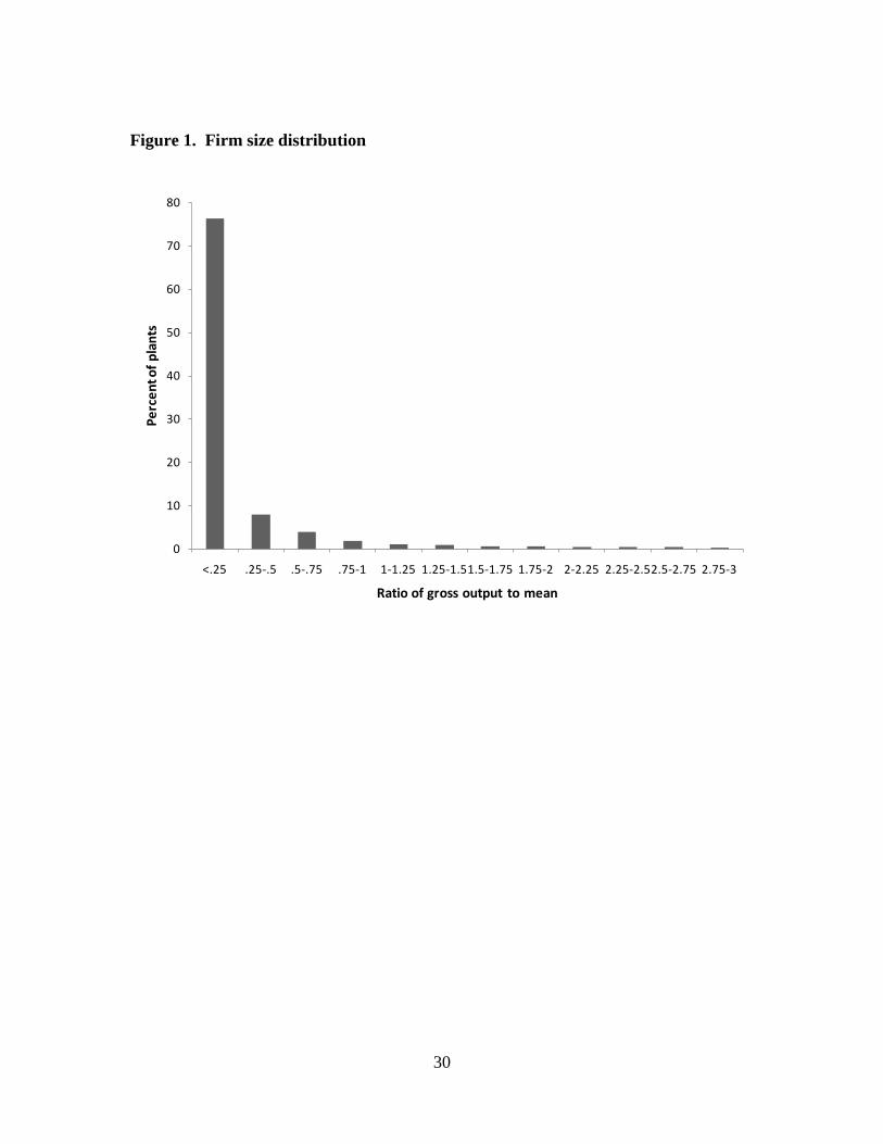
Second, we choose a functional form for the distribution of efficiency draws. We

follow Chaney (2008) in letting the distribution be Pareto:

( ) 1 ( / )G a a γθ= − , (25)

a θ≥ , where 0θ > and 1γ > . The size distribution of firms in the model is proportional

to the distribution of efficiency draws. As Figure 1 shows, the size distribution of plants

in the data is consistent with a Pareto distribution.

Third, we restrict our attention to the case where not all entering firms choose to

operate and not all operating firms choose to import. This leads to a characterization of

12

firms’ operating and technology decisions in terms of cutoff rules. We denote the cutoff

for operating by Na , where Na satisfies

( ) 0N Naπ = . (26)

We assume that Nφ is sufficiently large that Na θ> . We denote the cutoff for importing

by Ia , where Ia satisfies

( ) ( )I I N Ia aπ π= . (27)

We assume that Iφ is sufficiently large that I Na a> . Under these assumptions, there is

an exact analytic solution for the equilibrium, which we provide in Appendix 1. In

Appendix 2, we provide the solution under the assumption that the economy is in autarky.

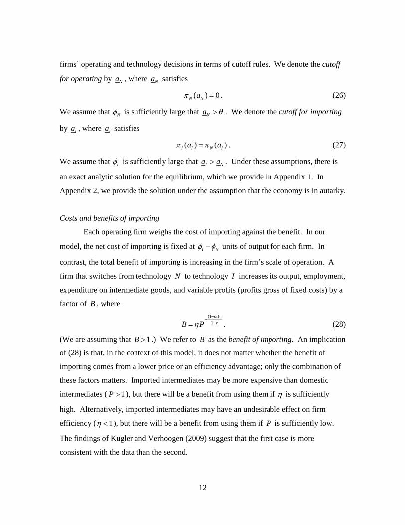
Costs and benefits of importing

Each operating firm weighs the cost of importing against the benefit. In our

model, the net cost of importing is fixed at I Nφ φ− units of output for each firm. In

contrast, the total benefit of importing is increasing in the firm’s scale of operation. A

firm that switches from technology N to technology I increases its output, employment,

expenditure on intermediate goods, and variable profits (profits gross of fixed costs) by a

factor of B , where

(1 )

1B Pα ννη

−−

−= . (28)

(We are assuming that 1B > .) We refer to B as the benefit of importing. An implication

of (28) is that, in the context of this model, it does not matter whether the benefit of

importing comes from a lower price or an efficiency advantage; only the combination of

these factors matters. Imported intermediates may be more expensive than domestic

intermediates ( 1P > ), but there will be a benefit from using them if η is sufficiently

high. Alternatively, imported intermediates may have an undesirable effect on firm

efficiency ( 1η < ), but there will be a benefit from using them if P is sufficiently low.

The findings of Kugler and Verhoogen (2009) suggest that the first case is more

consistent with the data than the second.

13

Sources of differences between importers and non-importers

In the data, importers are very different from non-importers. In the model, there

are two causes of this: a selection effect and a technology upgrading effect. Because of

the fixed cost, only the firms with the highest efficiency draws choose to become

importers. This is the selection effect. If a firm chooses to use technology I , then its

output, employment, expenditure on intermediate goods, and variable profits are larger by

a factor of B than if the firm had chosen to use technology N . This is the technology

upgrading effect.

We can measure the contribution of each effect to the relative size of importers

(the measure of size can be gross output, employment, total expenditure on intermediate

goods, or variable profits). In the absence of any selection effect, technology upgrading

would result in importers being B times larger than non-importers. The selection effect

determines the extent to which the size ratio is greater than B . Let S be size of the

average importer relative to the size of the average non-importer. Using a logarithmic

decomposition to account for this ratio, the share due to the technology upgrading effect

is given by log / logB S ; the remaining share is due to the selection effect. Later, our

calibration procedure will pin down the magnitudes of these two effects.

Aggregate technological efficiency

Along with the benefit of importing, an important statistic in the model — it

shows up in the calculation of every equilibrium object — is

( )1 ( ) ( )I

N I

a

a aM

A adG a B adG aγφ

∞= +∫ ∫ . (29)

We refer to A as an aggregate technological efficiency index because the expression in

parentheses is a weighted average of firms’ efficiency draws. The relative weight on

importers, B , accounts for the benefit of using technology I . Implicitly, the weight on

firms that choose not to operate is zero. Since the cutoffs Na and Ia are equilibrium

14

objects, we can simplify (29) to express aggregate technological efficiency entirely in

terms of parameters:

1/1 1( 1) ( )

( 1)N I N

M

BAγγ γ γφ φ φθ

γ φ

− − + − −= −

. (30)

Aggregate technological efficiency affects many important aspects of the

economy. For example, aggregate output can be expressed as

1

A KLY

ναν

αν

−

= , (31)

where K is given in Appendix 1. The wage and the measure of entrants are also

proportional to (1 )/A ν αν− , as is social welfare if 0τ = . In addition, the cutoffs for

operating and importing are proportional to A :

N Na Aφ= (32)

( )1

I NI

AaBφ φ−

=−

. (33)

Notice that the cutoff for importing is increasing in the cost of importing and decreasing

in the benefit of importing.

Effects of tariff reduction, terms-of-trade improvement, and trade-cost reduction

In our experiments, we consider the effects of trade liberalization, as given by a

decrease in τ ; an exogenous improvement in the terms of trade, as given by a decrease in

p ; and a reduction in trade costs, as given by a decrease in Iφ . Since our model is static,

we view it as capturing the long-term effects of permanent changes. These three types of

changes have many qualitative effects in common.

Proposition. Tariff reduction, an improvement in the terms of trade, or a decrease in the

cost of importing has the following effects: (i) the cutoff for operating increases, (ii) the

cutoff for importing decreases, (iii) the (real) wage increases, (iv) output increases, (v)

firm entry increases, and (vi) social welfare increases.

15

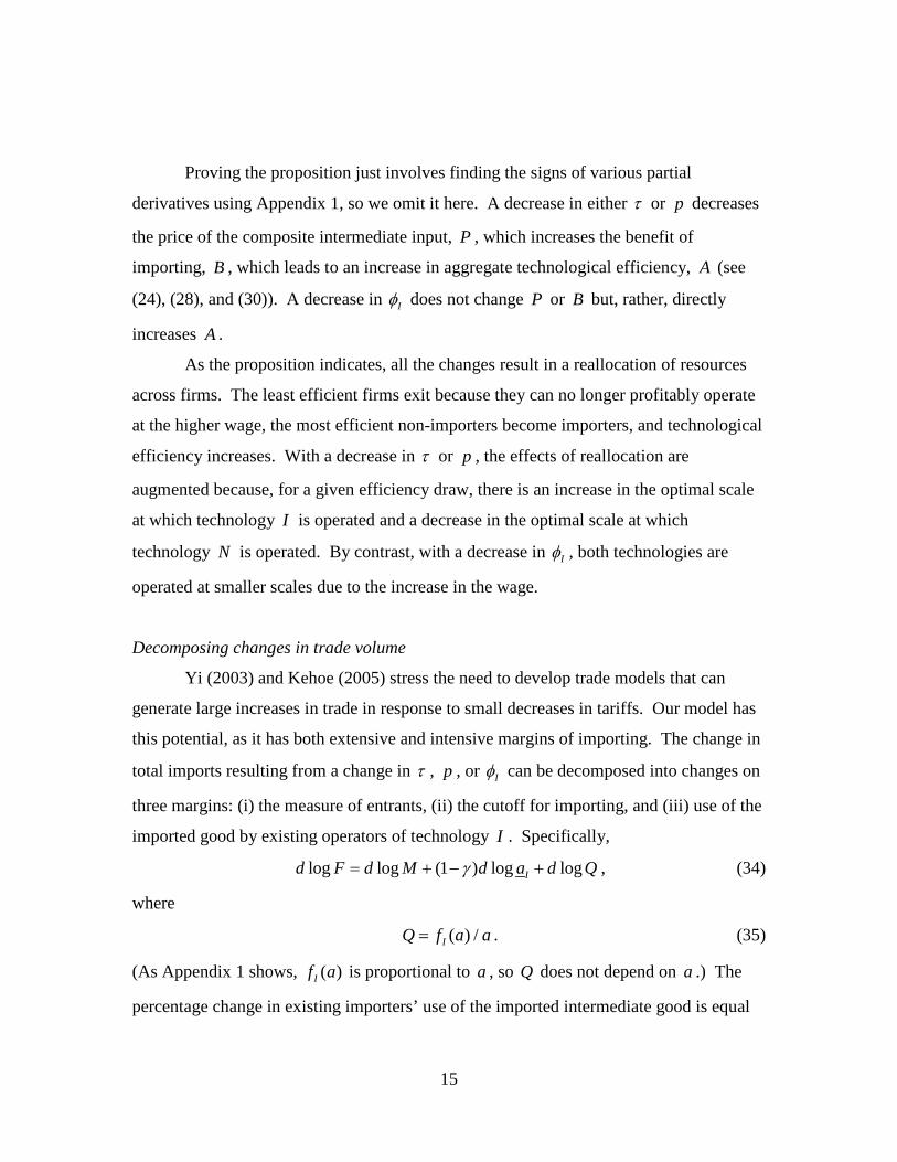
Proving the proposition just involves finding the signs of various partial

derivatives using Appendix 1, so we omit it here. A decrease in either τ or p decreases

the price of the composite intermediate input, P , which increases the benefit of

importing, B , which leads to an increase in aggregate technological efficiency, A (see

(24), (28), and (30)). A decrease in Iφ does not change P or B but, rather, directly

increases A .

As the proposition indicates, all the changes result in a reallocation of resources

across firms. The least efficient firms exit because they can no longer profitably operate

at the higher wage, the most efficient non-importers become importers, and technological

efficiency increases. With a decrease in τ or p , the effects of reallocation are

augmented because, for a given efficiency draw, there is an increase in the optimal scale

at which technology I is operated and a decrease in the optimal scale at which

technology N is operated. By contrast, with a decrease in Iφ , both technologies are

operated at smaller scales due to the increase in the wage.

Decomposing changes in trade volume

Yi (2003) and Kehoe (2005) stress the need to develop trade models that can

generate large increases in trade in response to small decreases in tariffs. Our model has

this potential, as it has both extensive and intensive margins of importing. The change in

total imports resulting from a change in τ , p , or Iφ can be decomposed into changes on

three margins: (i) the measure of entrants, (ii) the cutoff for importing, and (iii) use of the

imported good by existing operators of technology I . Specifically,

log log (1 ) log logId F d M d a d Qγ= + − + , (34)

where

( ) /IQ f a a= . (35)

(As Appendix 1 shows, ( )If a is proportional to a , so Q does not depend on a .) The

percentage change in existing importers’ use of the imported intermediate good is equal

16

to the percentage change in Q . Thus the first two margins are extensive, while the third

is intensive. Importantly, with the presence of extensive margins, the Armington

elasticity — the elasticity of substitution between domestic and imported goods — is

greater at the macro level than at the micro level. As a result, the model has the potential

to generate a large Armington elasticity at the macro level without assuming an unusually

large elasticity at the micro level.

Quantitative analysis

Here we calibrate the model using the data on the Chilean manufacturing sector

discussed earlier. Then we use the calibrated model to perform a number of

counterfactual numerical experiments.

Calibration

Our strategy for calibrating the model is as follows. First, we normalize certain

parameters that do not affect the quantitative findings in which we are interested. Then

we take some parameter values from the literature. Finally, we select the remaining

parameter values to match important statistics on plants’ importing behavior.

As normalizations, we set the labor endowment, L ; the lower bound on the Pareto

distribution, θ ; and the cost of entry, Mφ , to one. As (28) indicates, it does not matter

whether the benefit of importing comes from a lower price or an efficiency advantage.

Consequently, we normalize the price of the composite intermediate good, P , to one and

initially allow the size of the benefit of importing to be determined by the parameter η .

To obtain 1P = , we set the tariff rate, τ , to be consistent with the data and then choose

the relative price of the imported intermediate good, p . The World Bank’s World

dataBank reports that Chile’s average tariff rate in 2001 was 8 percent, so we set

0.08τ = . Then we set 0.11p = to obtain 1P = .

We take the values of ρ and ν from the literature. There is debate over the

elasticity of substitution between domestic and imported goods, the Armington elasticity.

Ruhl (2004) tries to resolve this debate and argues in favor of an elasticity of two at the

17

micro level (measurements at the macro level differ when an extensive margin is

involved). Following this, we set 0.5ρ = so that an importer’s elasticity of substitution

between domestic and foreign inputs is two. The parameter ν determines the degree of

decreasing returns at the firm level. Calibrating a competitive model with heterogeneous

firms operating decreasing-returns-to-scale technologies, Atkeson and Kehoe (2005) find

that 0.85ν = is consistent with data on U.S. manufacturing plants; we adopt this value

here.

The values of α and µ are selected to match expenditure shares in the data. In

the data, expenditure on labor as a share of expenditure on both labor and intermediate

goods is 0.34, so we set 0.34α = . Among plants that import, expenditure on imported

intermediate goods as a share of total expenditure on intermediate goods is 0.39; we set

0.78µ = to match this.

The remaining four parameters are the fixed cost of operating technology N , Nφ ;

the fixed cost of operating technology I , Iφ ; the TFP of technology I relative to

technology N , η ; and the shape parameter of the Pareto distribution, γ . We jointly

select the values of these four parameters so that the following four statistics hold in the

model: (i) 13 percent of operating plants use imported intermediate goods, (ii) the

average gross output of importers relative to non-importers is 4.5, (iii) the coefficient of

variation for gross output is 6.0, and (iv) 90 percent of entrants choose to operate.6

1.05Nφ =

The

resulting parameter values are , 1.66Iφ = , 1.21η = , and 2.02γ = . To place

these numbers in context, consider the following. The fixed cost of operating technology

N is 10 percent of the average non-importer’s gross output and 68 percent of its variable

profits. The fixed cost of operating technology I is 4 percent of the average importer’s

gross output and 24 percent of its variable profits. Since 1.21B = , switching from

technology N to technology I increases a firm’s gross output, employment, expenditure

on intermediate goods, and variable profits by 21 percent. Our value for the shape

6 The last statistic is not based on data (we do not observe plants that do not operate), but the quantitative results in which we are interested are not sensitive to the particular percentage chosen. We simply need the cutoff for operating to be binding.

18

parameter of the Pareto distribution is consistent with the findings of Del Gatto, Mion,

and Ottaviano (2007). Table 1 summarizes the calibration.

The calibrated model allows us to account for the average importer being 4.5

times larger, in terms of gross output, than the average non-importer. Using the

decomposition discussed in the previous section, with 1.21B = the share due to the

selection effect is 87.4 percent and the share due to the technology upgrading effect is

12.6 percent.

The calibration guarantees that the model satisfies Facts 1 to 3. We did not use

Fact 4 in the calibration, but the calibrated model is not far off. In the data, importers are

1.3 times more productive than non-importers, as measured by value added per worker.

In the calibrated model, importers are still substantially more productive than non-

importers, by a factor of 1.2. It is worth pointing out that the ratio would be one if we did

not take into account fixed costs of operation (as noted by Atkeson and Kehoe (2005)).

But our interpretation of the fixed costs is that they are expensed costs of setting up

business relationships with input suppliers, so they must be subtracted from gross output

to obtain value added. Though I Nφ φ> , expenditure on fixed costs relative to average

output is smaller for importers than non-importers. Consequently, measured value added

per worker is higher among importers than among non-importers. Table 2 provides a

comparison between the facts in the data and in the model.

Experiments

We use the calibrated model to perform four numerical experiments: (i)

elimination of the ad valorem tariff, (ii) an exogenous improvement in the terms of trade,

(iii) a reduction in fixed costs, and (iv) going from autarky to free trade.

We set up the first two experiments to be of the same magnitude. We consider (i)

the elimination of the 8 percent tariff in the benchmark calibration and (ii) an equivalent

reduction in the terms of trade (a 7.4 percent decrease in p ). Table 3 presents the

percentage changes in a number of statistics of interest. These two experiments have

almost identical quantitative results. The only differences are with respect to the changes

19

in exports, consumption, and tariff revenue. The main difference between the two

experiments is that the tariff reduction results in the loss of all tariff revenue, while the

terms-of-trade improvement increases tariff revenue. Our index of social welfare is the

consumption level. Because of the changes in tariff revenue, the welfare gain from tariff

elimination is much smaller than the welfare gain from the terms-of-trade improvement.

The terms-of-trade improvement allows the economy to import just as much as after the

tariff elimination, but without exporting as much output.

Both experiments result in a large increase in trade: the quantity of imports

increases by 98.8 percent. Using the decomposition given by (34), we find that 4.7

percent of the increase is due to the change in the measure of entrants, 69.7 percent is due

to the change in the cutoff for importing, and 25.6 percent is due to the change in existing

importers’ use of the imported intermediate good. Thus the extensive margins account

for the majority of the increase. In the benchmark calibration, of the firms that enter, 10

percent choose not to operate, 78 percent choose to operate technology N , and 12

percent choose to operate technology I . Following the change, entry increases by 3.3

percent and, of the firms that enter, 21 percent choose not to operate, 49 percent choose

to operate technology N , and 30 percent choose to operate technology I (see Table 4).

When there are extensive margins, the Armington elasticity at the macro level is

greater than the Armington elasticity at the micro level. Here the Armington elasticity at

the level of an individual firm is 2, while the measured aggregate Armington elasticity is

10.5. This large aggregate Armington elasticity is consistent with the empirical findings

of researchers who estimate it using data from trade liberalizations. As Ruhl (2004)

notes, these researchers typically find Armington elasticities ranging from 4 to 15. This

experiment makes clear that the extensive margins play an important role in generating

large increases in trade from small decreases in tariffs.

In addition to reporting how the changes affect our theoretical measure of

technological efficiency, we also report how they affect measured real GDP. To

calculate real GDP in our model in a manner similar to the way real GDP is calculated in

20

the data, we use base-period prices.7 t If we let denote the current period, then real GDP

at period-0 prices is

0 0 0 0(1 )t t t t N Nt I It tRGDP Y D p F M M p Fτ φ φ τ= − − + − − + , (36)

where NM is the measure of non-importers and IM is the measure of importers. The

first term is gross output, the next four terms are expenditure on intermediate goods and

expensed costs of operation, and the last term is the rebate of tariff revenue, all valued at

period-0 prices. We assume that investment in new firms is a tangible investment rather

than an intermediate input, so these expenditures are not subtracted from gross output.

The experiments result in a 1.5 percent increase in real GDP. In contrast to Kehoe and

Ruhl (2008), who find that terms of trade shocks have no first-order effect on real GDP in

a small open economy model with a representative firm, we obtain a substantial increase

in GDP by modeling heterogeneous firms and an extensive margin of importing.

The first two experiments involved increasing the benefit of importing. The third

experiment involves decreasing the fixed cost of importing, Iφ . To make this experiment

somewhat comparable in magnitude to the first two experiments, we select the percentage

decrease in Iφ so that the share of entrants that choose to operate technology I is the

same as after the previous two experiments (30 percent). This requires a 14.2 percent

decrease in Iφ . The results are presented in Table 3. Since B does not change in this

case, we can isolate the basic effects of reallocation. The increase in aggregate

technological efficiency is not as large as in the previous two experiments, so the changes

are mostly smaller in magnitude.

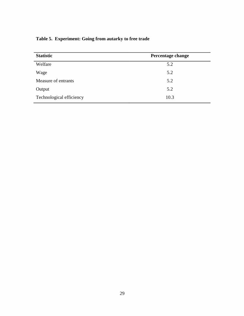
Finally, we consider the extreme case of going from autarky to free trade. In the

free trade case, we take the relative price of the imported good from the benchmark

calibration. This experiment puts an upper bound on the effects of tariff reduction alone.

The welfare gain is 5.2 percent. Table 5 presents the changes in some statistics of

interest.

7 See Gibson (2010), Kehoe and Ruhl (2008), and Bajona, Gibson, Kehoe, and Ruhl (2010) for further discussion of measured productivity and GDP in trade models.

21

Conclusion

Most trade models with heterogeneous firms emphasize firms’ export decisions.

We have developed a complementary approach that emphasizes firms’ import decisions.

Our model has desirable qualitative properties, is straightforward to calibrate, and

quantitatively captures many important features of plants’ importing behavior in the data.

In terms of policy implications, the welfare gains from unilateral trade liberalization may

not be large enough to persuade policymakers in countries that depend on tariffs for

revenue. Individuals associated with small non-importing firms are also unlikely to

support liberalization. Improvements in the terms of trade generate large welfare gains,

but are external. The simple modeling framework developed here allows for many

interesting extensions. These include the roles of dynamics, uncertainty, multiple

countries, monopolistic competition, and joint import-export decisions.

22

References

Amiti, M., and J. Konings. 2007. “Trade Liberalization, Intermediate Inputs, and

Productivity: Evidence from Indonesia.” American Economic Review 97:1611-

1638.

Atkeson, A., and P. J. Kehoe. 2005. “Modeling and Measuring Organization Capital.”

Journal of Political Economy 113:1026-1053.

Bajona, C., M. J. Gibson, T. J. Kehoe, and K. J. Ruhl. 2010. “Trade Liberalization,

Growth, and Productivity.” Ryerson University, Washington State University,

University of Minnesota, and New York University.

Bernard, A. B., J. B. Jensen, and P. K. Schott. 2009. “Importers, Exporters, and

Multinationals: A Portrait of Firms in the U.S. that Trade Goods.” In Producer

Dynamics: New Evidence from Micro Data, ed. by T. Dunne, J. B. Jensen, and M.

J. Roberts. National Bureau of Economic Research.

Castellani, D., F. Serti, and C. Tomasi. 2010. “Firms in International Trade: Importers’

and Exporters’ Heterogeneity in Italian Manufacturing Industry.” World Economy

33:424-457.

Chaney, T. 2008. “Distorted Gravity: The Intensive and Extensive Margins of

International Trade.” American Economic Review 98:1707-1721.

Del Gatto, M., G. Mion, and G. I. P. Ottaviano. 2007. “Trade Integration, Firm Selection,

and the Costs of Non-Europe.” CRENoS Working Paper.

Feenstra, R. C. 1998. “Integration of Trade and Disintegration of Production in the

Global Economy.” Journal of Economic Perspectives 12:31-50.

Gibson, M. J. 2010. “Trade Liberalization, Reallocation, and Productivity.” Washington

State University.

Gibson, M. J., and T. A. Graciano. 2011. “The Decision to Import.” American Journal of

Agricultural Economics 93:444-449.

Gibson, M. J., and T. A. Graciano. 2011. “Costs of Starting to Trade and Costs of

Continuing to Trade.” Washington State University.

23

Gopinath, G., and B. Neiman. 2011. “Trade Adjustment and Productivity in Large

Crises.” Harvard University and University of Chicago.

Halpern, L., M. Koren, and A. Szeidl. 2009. “Imported Inputs and Productivity.”

Hungarian Academy of Sciences, Central European University, and University of

California, Berkeley.

Helpman, E. 2006. “Trade, FDI, and the Organization of Firms.” Journal of

Economic Literature 44:589-630.

Hopenhayn, H. A. 1992. “Entry, Exit, and Firm Dynamics in Long Run Equilibrium.”

Econometrica 60:1127-1150.

Hummels, D., J. Ishii, and K.-M. Yi. 2001. “The Nature and Growth of Vertical

Specialization in World Trade.” Journal of International Economics 54:75-96.

Kasahara, H., and B. Lapham. 2008. “Productivity and the Decision to Import and

Export: Theory and Evidence.” University of Western Ontario and Queen’s

University.

Kasahara, H., and J. Rodrigue. 2008. “Does the Use of Imported Intermediates Increase

Productivity? Plant-Level Evidence.” Journal of Development Economics 87:106-

118.

Kehoe, T. J. 2005. “An Evaluation of the Performance of Applied General Equilibrium

Models of the Impact of NAFTA.” In Frontiers in Applied General Equilibrium

Modeling: Essays in Honor of Herbert Scarf, ed. by T. J. Kehoe, T. N. Srinivasan,

and J. Whalley. Cambridge University Press.

Kehoe, T. J., and K. J. Ruhl. 2008. “Are Shocks to the Terms of Trade Shocks to

Productivity?” Review of Economic Dynamics 11:804-819.

Kugler, M., and E. Verhoogen. 2009. “Plants and Imported Inputs: New Facts and an

Interpretation.” American Economic Review Papers and Proceedings 99:501-507.

Levinsohn, J. 1999. “Employment Responses to International Liberalization in Chile.”

Journal of International Economics 47:321-344.

Liu, L. 1993. “Entry-Exit, Learning, and Productivity Change: Evidence from Chile.”

Journal of Development Economics 42:217-242.

24

Melitz, M. J. 2003. “The Impact of Trade on Intra-Industry Reallocation and Aggregate

Industry Productivity.” Econometrica 71:1695-1725.

Muûls, M., and M. Pisu. 2009. “Imports and Exports at the Level of the Firm: Evidence

from Belgium.” World Economy 32:692-734.

Pavcnik, N. 2002. “Trade Liberalization, Exit, and Productivity Improvements: Evidence

from Chilean Plants.” Review of Economic Studies 69:245-276.

Ramanarayanan, A. 2007. “International Trade Dynamics with Intermediate Inputs.”

Federal Reserve Bank of Dallas.

Ruhl, K. J. 2004. “The International Elasticity Puzzle.” New York University.

Yi, K.-M. 2003. “Can Vertical Specialization Explain the Growth of World Trade?”

Journal of Political Economy 111:52-102.

25

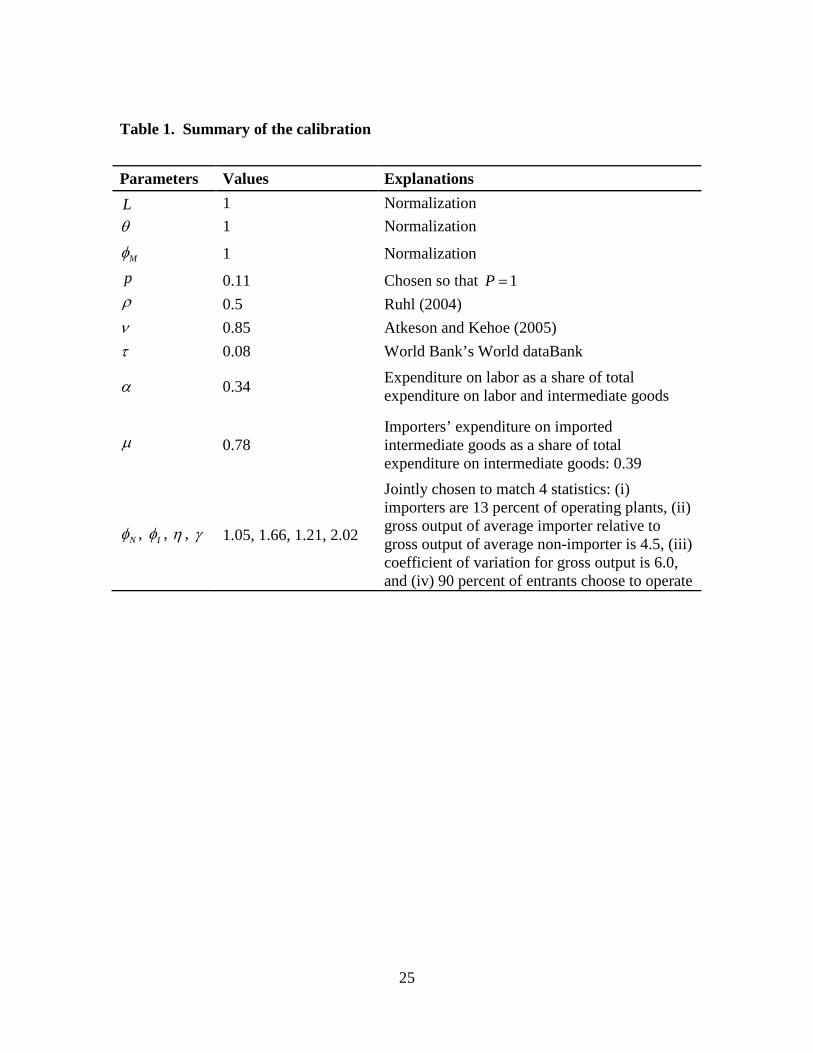
Table 1. Summary of the calibration

Parameters Values Explanations L 1 Normalization θ 1 Normalization

Mφ 1 Normalization p 0.11 Chosen so that 1P = ρ 0.5 Ruhl (2004) ν 0.85 Atkeson and Kehoe (2005) τ 0.08 World Bank’s World dataBank

α 0.34 Expenditure on labor as a share of total expenditure on labor and intermediate goods

µ 0.78 Importers’ expenditure on imported intermediate goods as a share of total expenditure on intermediate goods: 0.39

, N Iφ φ , η , γ 1.05, 1.66, 1.21, 2.02

Jointly chosen to match 4 statistics: (i) importers are 13 percent of operating plants, (ii) gross output of average importer relative to gross output of average non-importer is 4.5, (iii) coefficient of variation for gross output is 6.0, and (iv) 90 percent of entrants choose to operate

26

Table 2. Data vs. model

Statistic Data Model Importers as a share of operating plants (%) 13 13 Average importer’s expenditure on imported intermediate goods as a share of total expenditure on intermediate goods (%)

39 39

Gross output of average importer relative to average non-importer 4.5 4.5

Value added per worker of importers relative to non-importers 1.3 1.2

27

Table 3. Three experiments

Statistic Tariff

elimination (% change)

Terms-of-trade improvement

(% change)

Fixed-cost reduction (% change)

Welfare 1.0 5.1 2.4 Wage 3.3 3.3 1.1 Measure of entrants 3.3 3.3 1.1 Output 3.3 3.3 1.1 Tariff revenue −100.0 84.0 59.7 Real GDP 1.5 1.5 2.2 Price of composite intermediate −3.0 −3.0 0.0 Imports 98.8 98.8 59.7 Technological efficiency 6.4 6.4 2.2 Benefit of importing 12.2 12.2 0.0

28

Table 4. Entrants’ operating decisions (percentage shares)

Decision Benchmark Tariff elimination

Terms-of-trade

improvement

Trade-cost reduction Autarky

Not operate 10 21 21 14 3 Operate technology N 78 49 49 56 97

Operate technology I 12 30 30 30 0

29

Table 5. Experiment: Going from autarky to free trade

Statistic Percentage change

Welfare 5.2

Wage 5.2

Measure of entrants 5.2

Output 5.2

Technological efficiency 10.3

30

Figure 1. Firm size distribution

0

10

20

30

40

50

60

70

80

<.25 .25-.5 .5-.75 .75-1 1-1.25 1.25-1.51.5-1.75 1.75-2 2-2.25 2.25-2.52.5-2.75 2.75-3

Perc

ent o

f pla

nts

Ratio of gross output to mean

31

Appendix 1. Analytic solution with trade

Let

( )1

1 11 1 1(1 ) (1 )P p

ρρρ

ρ ρ ρµ µ τ

−−

−− − −

= + − +

(37)

(1 )

1B Pα ννη

−−

−= (38)

11 1( 1) ( )

( 1)N I N

M

BAγ γ γ γφ φ φθ

γ φ

− − + − −= −

(39)

1 1 1

(1 ) (1 )Kν α

α αν αν ν α α− −

= − − . (40)

Then

(1 )( )(1 )N

ad aAν α

ν−

=−

(41)

1( )(1 )

Naa

A Kν αναν

αν

ν− +=

− (42)

( )(1 )N

ay aA ν

=−

(43)

( )N NaaA

π φ= − (44)

11 1(1 )( )

(1 )IaB Pd a

A

ρρ ρν α µ

ν

− −−=

− (45)

1( )(1 )

IaBa

A Kν αναν

αν

ν− +=

− (46)

( )1 1

1 11(1 )(1 ) (1 )( )

(1 )I

aB p Pf a

A

ρρ ρρν α µ τν

−− −−− − +=

− (47)

( )(1 )IaBy a

A ν=

− (48)

32

( )I IaBaA

π φ= − (49)

1

w A Kν

αν−

= (50)

N Na Aφ= (51)

( )1

I NI

AaBφ φ−

=−

(52)

1

(1 )

M

A KLM

ναν νανγφ

−

−= (53)

1

A KLY

ναν

αν

−

= (54)

( )

111 1 11 1

1 1

(1 ) 1 ( 1) ( )

( 1) ( )

N I N

N I N

A KL P B B

DB

ρνγ γ γρ ραν

γ γ γ

α φ µ φ φ

α φ φ φ

−− − −− −

− −

− + − − − =

+ − − (55)

( )( )

11 11 11 11

1 1

(1 )(1 ) (1 ) ( 1) ( )( 1) ( )

I N

N I N

A KL p P B BF

B

ρνγ γρ ραν ρ

γ γ γ

α µ τ φ φα φ φ φ

−− − −− −−

− −

− − + − −=

+ − − (56)

( )( )

11 11 11 11

1 1

(1 )(1 ) (1 ) ( 1) ( )( 1) ( )

I N

N I N

A KLp p P B BX

B

ρνγ γρ ραν ρ

γ γ γ

α µ τ φ φα φ φ φ

−− − −− −−

− −

− − + − −=

+ − − (57)

( )( )

11 11 11 11

1 1

(1 )(1 ) (1 ) ( 1) ( )( 1) ( )

I N

N I N

A KL p p P B BT

B

ρνγ γρ ραν ρ

γ γ γ

τ α µ τ φ φα φ φ φ

−− − −− −−

− −

− − + − −=

+ − − (58)

( )( )

1 11 11 11 1

1 1

(1 )(1 ) (1 ) ( 1) ( )1

( 1) ( )I N

N I N

p p P B BC A KL

B

ργ γρ ρν ρ

ανγ γ γ

τ α µ τ φ φα φ φ φ

− − −− −− −

− −

− − + − −

= + + − −

. (59)

33

Appendix 2. Analytic solution under autarky

Let

11

( 1)N

M

Aγ γφθ

γ φ

− = −

(60)

1 1 1

(1 ) (1 )Kν α

α αν αν ν α α− −

= − − . (61)

Then

(1 )( )(1 )N

ad aAν α

ν−

=−

(62)

1( )(1 )

Naa

A Kν αναν

αν

ν− +=

− (63)

( )(1 )N

ay aA ν

=−

(64)

( )N NaaA

π φ= − (65)

1

w A Kν

αν−

= (66)

N Na Aφ= (67)

1

(1 )

M

A KLM

ναν νανγφ

−

−= (68)

1

A KLY

ναν

αν

−

= (69)

1

(1 )A KLD

ναν α

α

−

−= (70)

1

C A KLν

αν−

= . (71)