0

Trade, Endogenous Quality, and Welfare in Motion Pictures

Fernando Ferreira

The Wharton School University of Pennsylvania

Amil Petrin

Department of Economics University of Minnesota and NBER

Joel Waldfogel

Carlson School, Department of Economics, and Law School University of Minnesota and NBER

September 19, 2012

Trade benefits consumers and producers, and the effects of trade can operate through product quality: larger markets can have greater investment and therefore higher quality products. We explore this channel in the movie industry, where quality is produced exclusively with sunk costs, these sunk costs are high, and international revenue is important. We develop a structural econometric model of the global movie market, which we use to document that half of world consumers’ – and virtually all of US consumers’ – gains from trade operate through quality. We also analyze the counterfactual impact of the elimination of European film subsidies.

We are grateful to the Carlson School’s Dean’s Small Research Grant program for funding and to Imke Reimers for excellent research assistance. We thank Julie Mortimer and seminar participants at the February 2012 NBER IO meetings at Stanford for comments. All errors are our own.

1

In the usual way that economists and policymakers think about trade, the benefit of

importing is that consumers in the importing country get access to a wider variety of products.

The benefit of exporting accrues to domestic sellers, who generate higher profits by selling their

products to a larger population of consumers. So, for example, when Hollywood movies are

made available in France, French consumers have access to Hollywood fare as well as domestic

French cinema and US film producers gain additional revenues. While all of this is true, it

misses an important feature of products made with investments in sunk costs. With large sunk

costs, an enlarged market can lead to larger investments in products and therefore higher quality

products.1

The movie industry is an auspicious context for exploring this phenomenon for a variety

of reasons. First, quality is produced primarily with sunk costs in this industry, and these

endogenous sunk costs are high. Major US movie releases cost an average of nearly $100

million dollars per film, and US producers spent about $20 billion on film production in 2007,

nearly two thirds of the world total. Second, international revenue is needed to finance current

US investment levels as most of Hollywood movies’ box office revenue is generated outside the

United States. In 2009, domestic revenue for major US releases was $10.6 billion while foreign

revenue was $19.3 billion, making it appear likely that US and foreign consumers of big-budget

movies experience substantial benefits from the quality investments made possible by trade.

Thus an important additional benefit of trade operates through the endogenous quality

channel as consumers both at home and abroad can have access to higher quality goods than they

would otherwise have without trade.

1 See Sutton (1991). We note at the outset that for us, as for Sutton, the term, “quality” simply means whatever determines the level of demand. Our use of the term is separate from its aesthetic connotations in common usage which, we understand, are particularly strong for cultural products such as movies and music.

2

The goal of this paper is to develop a model of the world movie market, which we put to

two uses. First, we quantify the gains from trade and measure the portion of these gains

operating through investments in quality. To the best of our knowledge, we are the first to

quantify the components of trade’s benefit operating through the endogenous quality channel.

Second, we use the model for policy simulation. Various public policies around the world seek

to affect the movie industry by subsidizing production costs, in part to correct a perceived market

failure arising from the under-provision of movies highly valued by small national audiences

(see Spence (1976)). For example in Europe one-third of the roughly $5 billion annual film

investment is financed with government subsidies. We simulate the impact on both consumer

and producer welfare in Europe and elsewhere from removal of these subsidies.

We estimate a structural model of movie demand using data on movie-specific box office

revenue and country-year data on ticket prices and per capita income. Our data include 6,672

movies in 14 countries over the years 2005-2009, which allows us to estimate country-by-movie

specific preferences, so that a French viewer (e.g.) can value any particular French movie

differently from a U.S. viewer. We then combine measures of product quality derived from

demand estimation with direct data on movie investment – production budgets for major releases

– to estimate the quality production function for movies. We use the production function

estimates in conjunction with the demand model to develop an expression for each country’s

profits, which depend on both its own movie budgets and the budget levels chosen in other

countries. We solve for a Nash equilibrium in investment – and associated surplus measures –

which serves as the model’s baseline. We then re-solve the model to estimate country-specific

changes in consumer and producer surplus under the counter-factual policy regime.

3

We find that movie trade benefits consumers everywhere. For consumers outside the US,

roughly half of the gain from trade stems from increases in product quality. Almost all of trade’s

benefit to US consumers operates through the higher quality of US movies made possible by

trade. Trade’s impacts on producers are more varied. Trade helps US producers but hurts

producers elsewhere. For the most part, movie investment in one country is a strategic substitute

for investment elsewhere. There are exceptions: for example, the optimal Hollywood response

to increased investment in much of Europe or the UK is an increase in investment.

We find that the elimination of European film subsidies would reduce European film

investment, harming European consumers and producers while aiding US producers. Because

reduced European investment would prompt reduced US investment, US and world consumers

would suffer slightly as well from the elimination of European subsidies. More generally, we

find that allowing for idiosyncratic consumer taste for movies is important for both the demand

model estimates and the flexibility of the comparative statics. Models that rule out systematic

taste heterogeneity for movies promote a finding of strategic substitutes by eliminating terms

related to strategic complementarity, as we show in the appendix.

The paper proceeds in five sections after the introduction. Section 1 provides facts about

world movie trade to substantiate the basic idea of the model: a) that the large US investment in

movies produces higher product quality in the eyes of US and foreign consumers, and b) that the

current level of investment is made possible only by both domestic and foreign revenue. Section

1 also discusses major policy interventions in the movie market as well as literature relevant to

the current project. Section 2 presents our model of the world movie market, including a model

of movie demand, a production function for movie quality as determined by budget levels, and

our equilibrium notion. Section 2 also discusses a key determinant of the model’s comparative

4

statics, whether movie investment in one country is a strategic substitute or complement for

investment in another. Section 3 describes the main data sources and presents some patterns in

the trade data. Section 4 presents the model estimates. Section 5 describes the results of the

simulation exercises, including a) estimates of the strategic investment relationship among

various country pairs, b) calculation of both the gains from trade and the portion operating

through quality, and c) a counterfactual simulation of the elimination of European film subsidies.

I. Trade and Investment in Motion Pictures

This section provides background in the forms of a) the magnitude of investment and

international revenue, b) the relationship of box office revenue to total industry revenue, c) a

discussion of policy interventions in world movie trade, and d) the existing literature.

1. Investment and International Revenue

As with other recorded media products – music, books, newspapers – the quality of

movies is determined by expenditures on sunk costs. Around the world, investments in sunk

costs on movies differ substantially. When compared with the rest of the world, the US motion

picture industry spends a large amount making movies, both overall and on a per-movie basis.

There are two different measures of aggregate movie budgets circulated in the movie

industry. The Motion Picture Association of America reports the average budgets of its

members’ movies. These members are the major studios and they collectively release roughly

200 movies per year. For example, the MPAA in 2005 reported that the average cost of

5

producing a member movie was $96.2 million. Members released 198 movies in 2005 leading to

an overall investment in US movies that was just over $19 billion in 2005.

Screen Digest provides movie production statistics for both the US, Europe, and Japan

using a broader set of movies. In 2007, for example, they report that the US produced 656

movies at an average cost of $31.0 million per movie for a total investment of $20.3 billion.2

On a per-movie basis, using the Screen Digest data, the US outspends other countries by

a substantial margin. In 2007 the average US movie budget was $31 million, compared with

$12.8 million in the UK, $14.7 in New Zealand, $9.1 million in Germany, $8.7 million in

Canada, and $7.2 million in France. Regardless of the data source used, it is clear that US

investment is large relative to the movie investment of other countries, both per movie and

overall.

As

Table 1 shows, the Screen Digest data indicate that worldwide investment in movie production

was $32.3 billion in 2007. Of this amount, nearly two thirds ($20.3 billion) was spent in the US.

Other countries with relatively high investments in movies include Japan ($2.0 billion), the UK

($1.5 billion), France ($1.6 billion), Germany ($1.1), Spain, ($0.6), Italy ($0.4), Canada (1.0) and

South Korea (0.5).

High US investment has been facilitated in part by innovative movie marketing practices.

As Waterman (2005) argues, US producers pioneered the price-discriminatory practice of

releasing movies in a sequence of exhibition “windows,” first showing films in theaters, then

releasing them for rental and home video purchase, later releasing them to pay television, and

finally to free television. By exploiting this strategy earlier than other countries, the US

2 The MPAA figure for 2000 = $16.2 billion overall and $10.8 billion including only production costs. Hence the Screen Digest figure includes only production costs.

6

producers were able to justify larger investments in movie budgets which, in turn, have made US

movies appealing in foreign markets as well.

Much of the revenue that US movies generate comes from abroad. According to the

MPAA, its members’ movies earned $10.6 billion at the US box office – and an additional $19.3

billion abroad - in 2008. Our data demonstrate this point as well both for US repertoire as well

as the repertoires of many other countries. While we describe our data in detail below, the last

column of Table 1 provides some preliminary evidence. For this table we assign each 2008

movie to an origin country based on its first listed country of origin. We then aggregate both

domestic and foreign (actually, sample-wide) box office revenue by origin country. The table

shows, for example, that US repertoire generated $17.5 billion in box office revenue in 2008, 52

percent of which was generated outside the US. Other countries – notably the UK, Australia,

and Hong Kong – generated even larger shares of their revenues abroad: 85, 84, and 83 percent,

respectively. Many countries generate a third or more abroad: France, China, Spain, and others.

2. Box Office Revenue, Total Revenue, and Investment

In this section we make two points. First, we show that foreign revenue is necessary for

covering production costs. If we total our estimates of the studios’ net proceeds from domestic

box office, home video, and various forms of television, we arrive at roughly $14 billion for

2000, a year in which total production costs for MPAA movies exceeded $16 billion. Second,

we document, to the extent that data allow, the relationship between what we do observe, box

office revenue, and the overall revenue remitted to the studios from all revenue sources, which

we cannot observe. Worldwide box office revenue in 2000 was roughly $13.8 billion. By

7

contrast, the studios’ proceeds from box office, DVD, and television was (very) roughly $20-$25

billion. Arriving at these conclusions requires a brief digression into motion picture accounting.

According to Vogel (2007) and Dale (1997), roughly a third of domestic box office

revenue is remitted to the studio. Roughly half of box office receipts are retained by the

exhibitor, and a third of the remainder (one sixth overall) is retained by the distributor.

Distributors retain slightly more when distributing US movies in foreign markets, 40 percent

rather than a third (Dale, 1997). Vogel (2007) estimates that US studios get $0.31 per dollar of

domestic box office revenue. Thus, of the $7.7 billion in domestic box office revenue in 2000,

the studios received $2.4 billion. Of the $13.8 billion in international box office, the studios

received roughly $5 billion.

Epstein (2010) emphasizes the large and growing roles of both home video (sales and

rental of tapes and now DVDs) and television. Based on confidential MPAA data, he reports

DVD sales of $13.1 billion in 2000.3

Data on television revenue are the most difficult to obtain. Epstein (2010) reports

worldwide 2000 television revenue of $15.5 billion. Inferring the domestic profit from that gross

Vogel (2007, p. 152) reports that of a $30 retail price, the

studio retains $8-$10. Thus, the studios’ proceeds from domestic home video in 2000 was

roughly $3.5 to $4.4 billion. (Later in the decade – in 2004 – domestic home video revenue

peaked at $22.8 billion and has since declined). According to Eurostat (2003), worldwide home

video sales totaled $24 billion in 2000. As a rough approximation – using Vogel’s estimate of

the studio proceeds – it appears that the studios received about $7 billion in worldwide proceeds

from home video.

3 See http://www.edwardjayepstein.com/MPA2007.htm, accessed May 12, 2010.

8

figure requires deductions for distribution fees, as well as a translation from a worldwide figure

to a US figure. Dale (1997, p. 319) reports that for both pay and free television, distributors

takes a “30-40 percent distribution fee plus marketing and distribution costs” which, in the case

of free television, are “minimal.” Putting the studio share of television revenue at two thirds, this

suggests that the studios’ net proceeds from television in 2000 were $10.3 billion.

These calculations lead us to our two conclusions. First, the studio proceeds from

domestic revenue sources are about $14 billion for 2000. Given that US production costs exceed

these revenues, we infer that international revenues are needed to finance current investments.

Second, studio proceeds from worldwide activities appear to total about $22 billion (5+7+10) in

a year when worldwide box office was almost $14 billion. Hence, as a rough approximation, it

appears that studio proceeds are about 1.5 times box office revenue. This translation is important

for us because we observe only theatrical box office, while profits actually depend on overall

revenue in relation to costs.

A strong correlation between box office and DVD revenue across title provides

justification for assuming proportionality between box office and total revenue. Because movies

are sold to broadcasters in bundles, there is essentially no evidence on movie-level television

revenue. We do have some movie-level DVD revenue data on the 100 top-grossing DVDs for

each year, 2007-2009, based on US sales, from http://www.the-numbers.com/, which we

matched with box office revenue from Box Office Mojo. For matching titles, the correlation

between domestic box office and domestic DVD sales is 0.76, as Figure 1 shows.4

3. Policy Interventions

4 Not all titles match, as the DVDs include some perennial sellers originally released much earlier (The Jungle Book), as well as some movies released only to DVD (such as the BBC series Planet Earth).

9

One of the major ways that policy affects movie trade is via state subsidies, which are

extensive in Europe. Table 2 describes these subsidies. In 2004 European film production

totaled $4.8 billion (according to Screen Digest, 2009), and subsidies accounted for nearly a third

of the total investment of $1.6 billion. In absolute terms the French spend the most on subsidies:

just under half of their $1.3 billion film investment in 2004 was financed by the state. Germany

provides the second largest subsidy: just above a third of their $0.7 billion film investment in

2004 came in the form of subsidies. The UK and Italy provided the next two largest in absolute

terms, accounting for 10 and 32 percent of those countries’ 2004 film investments, respectively.

Rationales for these subsidies include both economic and cultural factors. According to

the European Commission (in a discussion of its Creative Europe initiative), “Europe needs to

invest more in its cultural and creative sectors because they significantly contribute to economic

growth, employment, innovation and social cohesion. Creative Europe will safeguard and

promote cultural and linguistic diversity and strengthen the competitiveness of the cultural and

creative sectors.”5

4. Existing Literature

Perhaps because aspects of its performance are readily observed there is a substantial

scholarly literature on the film industry. Waterman has written extensively on many aspects of

the movie industry, including features relevant to trade such as the “cultural discount,” the extent

to which movies from one country appeal to consumers elsewhere. Much of this work is

summarized in Waterman (2005). DeVany (2003) has written extensively on the determinants of

5 See http://ec.europa.eu/culture/creative-europe/index_en.htm.

10

movie revenues. Einav (2007) analyzes the release timing game; and Einav and Orbach (2010)

study the puzzle of uniform box office prices. Davis (2006ab) and Chisholm and Norman

(forthcoming) describe spatial competition and in the exhibition market. Gil (forthcoming a, b)

provides analyses of vertical issues in movie making.

There is also a growing body of empirical work on trade in cultural products. Studies

include Hanson and Xiang (2008), Disdier et. al (2010)’s gravity model estimates, and Ferreira

and Waldfogel (forthcoming). Because of the importance of endogenous sunk costs in movies,

this work is related to Sutton (1991), as well as Berry and Waldfogel (2010). Related, movies

embody the preference externalities examined in Waldfogel (2003).

Methodologically, this work is related to research documenting the the welfare benefit of

new products (Petrin (2002) and Goolsbee and Petrin (2004)). Finally, this work is related to

other empirical industrial economic research examining product choices by consumers in

different national markets, such as Goldberg (1995) and Verboven (1996).

II. The Model

This section presents our models of demand and supply for the movie industry, as well as

equilibrium. We posit a logit, nested logit, and non-separable nested logit model for movie

demand.

1. Demand

The choice sets of movies vary both across countries and over time and not all movies

produced each year are available in all countries. Defining Jc as the set of movies available in

11

country c (with C total countries), we index movies by j (j=1,…,Jc , c=1,…C) and we suppress the

time subscript. We assume that every consumer decides in each month whether to see one

movie in the choice set Jc or to consume the outside good (not seeing a movie at a theater).

Specifically, every month every consumer i in country c chooses j from the Jc + 1 options that

maximizes the conditional indirect utility function given by:

𝑢𝑖𝑗 = 𝛽0 + 𝛼𝑝𝑐 + 𝜑𝑦𝑐 + 𝜉𝑐𝑗 + 𝜖𝑖𝑗 = 𝛿𝑐𝑗 + 𝜖𝑖𝑗,

where β0 reflects taste for movie theater patronage, α is the marginal utility of income, pc is the

price of a movie ticket in country c, yc is per capita income in country c, and φ measures how

tastes for movies vary with income. ξcj is the unobserved (to the econometrician) quality of

movie j from the perspective of country c consumers and can differ across countries for the same

movie (so Avatar e.g can have different quality to US vs French consumers). 𝜖𝑖𝑗 is a taste draw

that is distributed Type I extreme value and is independent across both consumers and choices.

With outside good utility 𝛿𝑐0 normalized to 0 for all 𝑗 ∈ 𝐽𝑐 the market shares are given by

𝑠𝑐𝑗 = 𝑒𝛿𝑐𝑗

1+∑ 𝑒𝛿𝑐𝑙𝐽𝑐𝑙=1

. Inverting out δcj from observed market shares as in Berry (1994) yields

ln(scj) – ln(sc0) = δcj = β0 + αpc + φyc + ξcj.

with δcj linear in the average country-level ticket price, per capita income, and ξcj.6

𝛿𝑐𝑗′ = 𝛿𝑐𝑗 − 𝛼𝑝𝑐 = 𝛽0 + 𝜑𝑦𝑐 + 𝜉𝑐𝑗.

Movie

quality 𝛿𝑐𝑗′ as measured by demand is then price-adjusted δcj:

In this model one might wish to instrument price because ξcj may be correlated with pc. 6 We observe country-specific market shares. This allows us to have the country-specific movie tastes for each product.

12

a. Nested Logit

A well-known drawback of the logit model is that it assumes that (𝜖𝑖0,𝜖𝑖1, … , 𝜖𝑖𝐽,)

are independently drawn across the Jc+1 choices. Full independence of individual tastes

precludes the possibility that consumers differ in their taste for watching movies at a theater. If

consumers have heterogeneous tastes, then estimated demand elasticities and substitution

patterns from the logit model will be biased, and this in turn will bias estimates of competitive

response and of consumer and producer welfare (Berry et. al (1995), Petrin (2002), Goolsbee and

Petrin (2004)).

One way to allow consumers to differ in their tastes is to put a random coefficient on the

intercept of the utility function:

𝑢𝑖𝑗 = 𝛽𝑖0 + 𝛼𝑝𝑐 + 𝜑𝑦𝑐 + 𝜉𝑐𝑗 + 𝜖𝑖𝑗,

where 𝛽𝑖0 represents a consumer-specific taste for movies relative to the outside good. In this

setup strong (weak) taste for one movie implies strong (weak) taste for other movies.

The nested logit model provides a computationally simple way to allow for this type of

random coefficient.7

where for consumer i ζi is common to all movies and has a distribution function that depends on

σ such that if 𝜖𝑖𝑗 is distributed extreme value, then [ζi + (1-σ) 𝜖𝑖𝑗] is also extreme value.

Nested logit posits utility

𝑢𝑖𝑗 = 𝛿𝑐𝑗 + ζ𝑖 + (1 − 𝜎)𝜖𝑖𝑗

8

7 It does not require the use of simulation-to-integrate to estimate market shares for different posited parameter values.

When

13

σ=0, the model resolves to the simple logit and ζi - the consumer-specific systematic movie-taste

component - plays no role in the choice decision. As σ approaches one, the role of the

independent taste shocks (𝜖𝑖0,𝜖𝑖1, … , 𝜖𝑖𝐽,) is reduced to zero, implying consumer tastes – while

different for any consumer i across movies – are perfectly correlated within consumer i across

movies.

Intuitively, identification of σ is driven by how the total inside share of movies changes

as the number of movies in the choice set varies. When σ is close to one, the total inside share

will not vary much with the number of movies, as additional movies simply cannibalize other

movies’ shares.9 At the opposite extreme, with σ=0, is the logit model, where some consumers

of the outside good will always substitute to a new movie when it is added to the choice set.10

The estimating equation for the nested logit is linear in the same arguments as the logit

and has a new explanatory variable which is the product’s share among inside goods ln(sj/(1-s0)):

ln(sjc) – ln(s0) = β0 + αpc + φyc + σln(sjc/(1-s0c)) + ξcj.

with σ the coefficient on the new explanatory variable. It will be positive if variation in a good’s

share relative to the total inside share (1 − 𝑠𝑐0) explains ln (𝑠𝑐𝑗/𝑠𝑐0) conditional on the other

8 The formula for the market share of good j is 𝑠𝑐𝑗 = 𝑒𝛿𝑐𝑗

1−𝜎�

(𝐷𝐽𝑐𝜎 +𝐷𝐽𝑐)

, where 𝐷𝐽𝑐 = ∑ 𝑒𝛿𝑐𝑗

1−𝜎�𝐽𝑐𝑙=0 .

9 For any given set of product qualities σ determines how the total inside good share of movies changes as the

number of products increases. Denoting the inside share as 𝑠𝐼𝐽 =

∑ 𝑒𝛿𝑙𝐽𝑙=1

1+∑ 𝑒𝛿𝑙𝐽𝑙=1

, the change in the inside share that arises

from adding a J+1th good with quality 𝛿𝐽+1 to the choice set is given by

Δ𝑠𝐼𝑛𝑠𝑖𝑑𝑒 = 𝑠𝐼𝐽+1 − 𝑠𝐼

𝐽 =𝐷𝐽𝜎𝐷𝐽+1−𝐷𝐽+1

𝜎 𝐷𝐽(𝐷𝐽

𝜎+𝐷𝐽 )(𝐷𝐽+1𝜎 +𝐷𝐽+1)

.

On the interval 𝜎 ∈ [0,1), Δ𝑠𝑖𝑛𝑠𝑖𝑑𝑒(𝜎) is everywhere positive and decreasing in σ. 10In the logit case Δ𝑠𝐼𝑛𝑠𝑖𝑑𝑒 = 𝑒𝛿𝐽+1

𝐷𝐽 𝐷𝐽+1which is always positive.

14

explanatory variables. The new regressor is a function of quantities and thus like price is also

endogenous. Price adjusted movie quality 𝛿𝑐𝑗′ is now given as:

𝛿𝑐𝑗′ = 𝛿𝑐𝑗 − 𝛼𝑝𝑐 − 𝜎𝑙𝑛(𝑠𝑐𝑗/(1 − 𝑠𝑐0)) = 𝛽0 + 𝜑𝑦𝑐 + 𝜉𝑐𝑗.

b. Nested Logit with Non-Separability

One shortcoming of the nested logit specification is that it is not able to accommodate

rotations in the demand curve due, for example, to advertising.11 Specifically, a separable

demand error does not allow unobserved advertising to affect the marginal utility of income.

We know that advertising budgets, while omitted from our measured budgets, are about half as

large as observed production budgets in the US (Vogel, 2007). If unobserved advertising

rotates the demand curve, then our standard IV approach is no longer consistent because the

instrumented price is correlated with the demand error, which now includes an interaction term

between price and the error.12

We explore this extension in the movie demand data here by estimating a nested logit

specification that allows price to interact with the demand error. We generalize the nested logit

utility specification to include an interaction term between price and the demand error:

ln(sjc) – ln(s0) = β0 + αpc + φyc + σln(sjc/(1-s0c)) + ξcj +λpcξcj.

This allows unobserved factors to both shift and rotate the demand curve.

2. Supply: the Production of Quality

11 A large empirical literature demonstrates that advertising can both shift and rotate the demand curve. See Pakes’ (1987) review of Mueller (1986). 12 Gandhi, Kim, and Petrin (2011) show an example in which price elasticities increase by 60% when the demand framework is generalized to allow for non-separable errors.

15

While our demand side estimates depend in no way on the supply side model, we require

a characterization of supply in order to conduct our counterfactuals. In principle, film producers

have two margins of adjustment. They can make more movies, or they can spend more on the

movies that they make. Our model below makes the simplifying assumption that budgets are the

only margin employed, an assumption that is consistent with our historical data.13

Each year the movie industries of each country invest in slates of movies. We posit that

the quality of the movies depends in part on the size of the production budgets. Using the

estimated price-adjusted qualities from the demand system as the dependent variable, we recover

the production relationship by relating δ’ to observed budgets and controls:

𝛿𝑐𝑗′ = 𝛾 log�𝐵𝑗� + 𝜇𝑐 + 𝜇𝑡 + 𝜖𝑐𝑗

This

assumption also allows us to sidestep the problem of how to model the quality of as-yet non-

existent goods, a generic problem that has not yet been solved in the literature.

where γ is the return to budget investment and the fixed effects for destinations and time are

given as μc and μt, respectively. In principle this equation could include a dummy for country of

origin as well, but in practice our data on movie-level budgets are predominantly from the US.

While we restrict γ to be common across destination countries, with sufficient data we could

allow γ to be indexed both by importing and exporting country. Movie budgets may be

endogenous, and we describe instrumental variables strategies in the empirical section.

3. Nash Equilibrium and Revenue Weights

13 For example, in the United States, the total budget on major MPAA releases has grown from $35 million to $100 million per film in constant 2005 dollars between 1980 and 2005, while the number of releases has been roughly stable (see Figure 2).

16

Define rcj(𝛿𝑐𝑗′ (𝐵𝑗),𝛿−𝑐𝑗′ (𝐵−𝑗)) as the revenue from movie j in destination country c,

where we explicitly note its dependence on the qualities of all movie available in country c. That

is, rcj depends on the size of j’s budget as well as the size of all other movies’ budgets. The

worldwide profit for movie j is then its revenue in all countries less its budget:

∑ 𝑟𝑐𝑗�𝛿𝑐𝑗′ (𝐵𝑗),𝛿−𝑐𝑗′ (𝐵−𝑗)� − 𝐵𝑗𝐶𝑐=1 .

In practice – and as discussed above – box office is one of three major revenue sources,

along with home video and television. Because we do not observe all of these, we need to

estimate the relationship between box office revenue and producers’ net proceeds from all

sources. We do this by allowing for a producer-specific scale factor Wj, so 𝑟𝑐𝑗 = 𝑊𝑗𝑟𝑐𝑗′ , where

r’( ) contains only box office revenue. Total profits for movie j are given by

∑ �𝑊𝑗𝑟′𝑐𝑗�𝛿𝑐𝑗′ (𝐵𝑗), 𝛿−𝑐𝑗′ (𝐵−𝑗)� − 𝐵𝑗�𝐶𝑐=1 ,

We then use the first-order conditions for profit maximization to estimate these weights.

Producers typically have multiple products. For a decision maker responsible for a set of

movies F, profit from box office revenues is given by:

∑ ∑ �𝑊𝑗𝑟′𝑐𝑗�δcj′ (Bj), δ−cj′ (B−j)� − Bj�𝐶𝑐=1𝑗∈𝐹 .

Given the ticket price and market size in each country, along with the preferences of

consumers for the set of products , we assume that firms compete Nash in budgets, and we solve

for the Wj’s that satisfy the Nash equilibrium conditions at the box office revenues and budgets

in the data. We then use these estimated values of Wj in the profit functions for policy

17

counterfactuals. For our policy counterfactuals we can modify either the revenue or budget

function (or both) and resolve for the new Nash equilibrium.

a. Strategic Substitutes and Strategic Complements

Changes in budgets across the counterfactuals will be determined in part by the collective

competitive investment responses of players to one another, as in Bulow, Geanakoplos, and

Klemperer (1985). In our context a player is an entity controlling budgets for a set of movies,

and the competitive response of player 1’s budget to changes in player’s 2 budgets will depend

on how the derivative of player 1’s profits 1Π with respect its budget 1B changes as player 2’s

budget 2B changes:

1

2 1B B ∂Π∂ ∂ ∂

If it is positive (negative) then investment decisions are strategic complements (substitutes), as

increases in player 2’s budget increase (decrease) the marginal profitability of an extra dollar of

investment by player 1, leading player 1 to respond with more (less) investment. As we show in

the appendix, ruling out idiosyncratic heterogeneity in tastes for movies, as the simple logit

model does, tends to bring about a finding of strategic substitutes by eliminating terms related to

strategic complementarity. Specifically, the more highly correlated are consumer tastes across

movies – a higher σ in our setup – the easier it is to steal market share from competitors by

increasing one’s own movie quality.

III. Data

18

The basic data for this study are the market shares of 6,672 movies in 14 distinct

countries between 2005 and 2009, for a total of 16,189 movie-country-year observations. In

addition we observe ticket prices and per capita income by country and year, not at the level of

the individual movie. The market shares are derived from box office revenue data which in turn

were obtained from Box Office Mojo (boxofficemojo.com). The ticket price data, along with

data on overall country film investment are obtained from Screen Digest.

Movie-level budget data for 770 major releases (and 5,223 movie-country observations)

are obtained from www.thenumbers.com, which reports estimates of production budgets for

major films.14

Before turning to the modeling, the simple tabulations from the data are of some interest.

Tables 3 and 4 show patterns of world trade in movies in 2008. Table 3 shows where each origin

country sells its repertoire. Table 4 shows the national origins of each destination country’s

consumption. These two tables answer the respective questions, “who buys my repertoire?” and

“whose products do our consumers like?” that are central to the way that, say, trade policies

would affect equilibrium trade patterns.

Data on European film subsidies in 2004 are obtained from Cambridge

Econometrics (2008).

For example, Table 3 shows that domestic markets are important outlets for all

repertoires. Domestic sales account for three quarters of sales for the repertoires from Brazil,

France, Germany, India, Italy, Japan, Mexico, South Korea, and Turkey. The Anglophone

countries (Australia, the UK, and US) are different: domestic sales account for half of US sales

and under a fifth of Australian and UK sales. Those repertoires instead achieve substantial sales

14 Budget data are also reported at boxofficemojo.com. Both data sources report production budget information for only a subset of movies. It appears to be essentially the same subset.

19

in the other Anglophone countries, chiefly the US. They also obtain atypically high shares of

their sales in other countries.

Table 4 shows which repertoires consumers in each destination market choose. Two

patterns are clear. First, there is a home market effect: the main diagonal entries are large.

Countries with particularly large apparent preferences for domestic product include India (77

percent), Japan (59), Turkey (52), and the US (90). Second, Anglophone countries’ – especially

the US and the UK – have high market shares everywhere. France, too, has relatively high

market shares, particularly in Europe.

The information in Tables 3 and 4 is interesting and provides some hints about how

counterfactual policies might affect welfare outcomes. It is clear that consumers in many

countries would be made worse if they lost access to US movies. It is also relatively clear that

US consumers would not suffer much from loss of access to foreign movies. But the raw data

cannot provide estimates of the welfare impact of the lower investment level that would prevail

without trade. Hence the need for an explicit model simultaneously endogenizing all countries’

investment decisions.

IV. Empirical Implementation

Table 5 reports estimates of the demand models and Table 6 includes the implied

elasticities. We include each country’s average income as an explanatory variable to capture

unobserved heterogeneity in tastes that is correlated with income, as suggested by McFadden

(1982). Estimates of the coefficient on price and the inside share along with the market shares

of each movie are sufficient to calculate the quality δ′ of each movie in each market.

20

We have two types of instruments that we use for price and the inside share. The

literature has made wide use of the assumption from Berry et. al. (1995) that product

characteristics are exogenous. In our setting under this assumption the total number of movies is

a valid instrument so we use the log of the number of movies released in each country-year.15

We also use the Hausman (1994)-style instruments, where prices in other locations are valid

instruments if they reflect common worldwide cost shocks to making movies like changes in

technology.16

The first column reports the simple logit model with price assumed to be exogenous. As

Table 6 indicates, the implied mean (median) movie-level price elasticity of demand is -2.25

(-2.43) and the implied overall price elasticity for movies when considered together (the inside

elasticity) is -1.87 (-2.00). Columns (2) and (3) of Table 5 report the nested logit estimates with

price assumed exogenous and the inside share instrumented with the BLP instrument (2) and the

Hausman instrument (3) respectively. The estimates are markedly different from the simple

logit, but they are very similar across these two specifications. The price coefficient is about

60% of its logit magnitude (-0.17 and -0.18) and the substitution parameter (σ) is highly

significant and close to one (0.795 and 0.821), indicating a high degree of substitutability of

among movies. The consequence for the demand estimates relative to the logit model is that the

resulting mean movie-level price elasticities are much higher in absolute value, at -5.42 in both

specifications, while the inside share elasticities are slightly lower. Thus the nested logit models

We use functions of the average ticket price in other countries as instruments for

the home-country price. Finally, in some of the specifications we treat price as exogenous

because it is the average price across movies and not the movie- specific price.

15Recall that identification of the idiosyncratic taste parameter is related to how inside shares change and the number of movies available in a market changes 16 If there are worldwide demand shocks like international advertising campaigns that are correlated with price and affect demand then this instrument will be correlated with the demand error.

21

suggest that there is a set of consumers with very strong preferences for going to the movies, but

who are readily willing to substitute between movies in response to small increases in one

movie’s price holding other movies prices constant.

In the fourth column of Table 5 we treat both price and the inside share as engodenous

using both types of instruments. Column 5 treats both as endogenous and uses the approach

described in Gandhi, Kim, and Petrin (2011) to allow for possible interactions between price and

unobserved (to us) advertising. In both cases the coefficients and implied elasticity estimates are

similar to columns 2 and 3. We use the demand estimates in column (2) for our counterfactuals,

but we note that the estimates in the subsequent columns are very similar.

2. The Quality Production Function

A key relationship in our model is the link between budgets and quality. We have

country-specific measures of each movie’s quality (δ’) from the demand model, and we have

budget data on 770 major releases (mostly from the US). Figure 3 presents the relationship

between quality and log budget, separately for four major destination markets, derived from the

nested logit model. The relationships are positive, indicating that movies with higher production

budgets tend to have higher perceived quality. We have 4,221 observations for which we

observe the identity of the studio making the movie. We use this subset for analysis.

Our simplest quality production function relates our measure of movie quality to the log

production budget of the movie. We include year dummies to account for the fact that the

sample contains movies from different years (and that input prices may be changing over time).

We also include destination dummies, allowing for the possibility that audiences in different

22

countries like the largely US movies in the sample to different extents. The resulting coefficient

on log budget, in column (1) of Table 7, is 0.160 (se=0.0042 ).

We would like to control for non-budget aspects of the movie quality. One possible

determinant of quality is the identity of the studio producing the movie. Different studios may

have different movie-making acumen, which would give rise to different quality for a given level

of budget. Different studios may also have different distribution capabilities, which would

generate different revenue – and therefore implied quality – than others. When we include a

studio fixed effect along with year and destination fixed effects, the coefficient on log budget

changes slightly, to 0.162 (see column (4)).

We are concerned that budgets may be endogenous. For example, movies based on a

better concept may attract both larger audiences and greater investment, which could be mistaken

for a causal relationship between investment and quality. To get a causal estimate of the

parameter γ we need a source of variation in budgets that is not contaminated by movie quality.

For this we appeal to the idea that studios that are flush with cash will invest more, an idea

reminiscent of a robust empirical relationship in corporate finance.17

Column (2) reports a first-stage regression of log budgets on last year’s revenue and

budgets for the studio. Including year and destination effects but not studio fixed effects, the

revenue coefficient is positive, which accords with our prior. However, the lagged budget

We also posit that studios

that spent large budgets in the previous year may be constrained in their current year spending.

Thus we instrument a studio’s current movie budgets using its revenues and budgets from the

previous year.

17See Fazzari, Hubbard, and Peterson (1988) and the large related literature.

23

coefficient is also positive, which is inconsistent with our prior. The resulting IV estimate of the

log budget coefficient, in column (3), is 0.171.

Column (5) reports a first-stage regression of log budgets on last year’s revenue and

budgets for the studio, including studio fixed effects, generating a positive and significant lagged

revenue coefficient and a negative and significant lagged budget coefficient. The resulting IV

estimate of the log budget coefficient, in column (6), is 0.189. Hence, all of these specifications

yield rather similar estimates of the log budget coefficient, between 0.16 and 0.19. We proceed

with the column (1) estimate.

We observe movie-specific revenue in each sample country but we observe movie-

specific budgets only for the major releases, most of which are from the US. For the remainder

of the world, we observe aggregate annual country investment in movies. We adapt our

implementation accordingly by modelng the decision making at the level of eleven groups of

countries: the Australia, China, France, Germany, Italy, Japan, South Korea, Spain, the UK, the

US, and a composite rest-of-the-world. This has two implications. First, we model

counterfactual quality as the following functions of budgets:

𝛿𝑐𝑗′ �𝐵𝑗� = 𝛿𝑐𝑗0′ + 𝛾log (𝐵𝑗 𝐵𝑗0)⁄ .

For us, the sets of movies are the movies from each of the 11 origin regions. Thus, we model as

observed quality (𝛿𝑐𝑗0′ ) plus the percent change in budget for that origin country (α) times the

common production function parameter linking investment to quality (γ). Second, the weights W

that translate box office revenue into producer revenue are also calculated at the level of the

origin region.

24

V. Model Simulations

1. Baseline Simulation

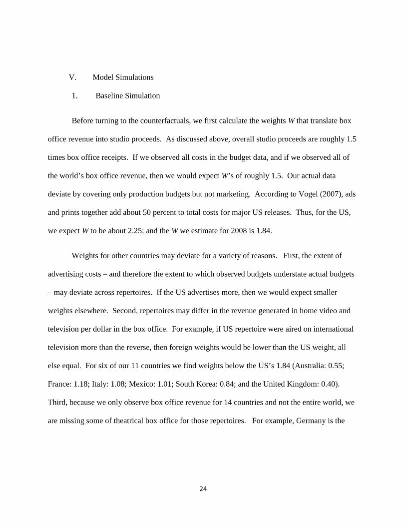
Before turning to the counterfactuals, we first calculate the weights W that translate box

office revenue into studio proceeds. As discussed above, overall studio proceeds are roughly 1.5

times box office receipts. If we observed all costs in the budget data, and if we observed all of

the world’s box office revenue, then we would expect W’s of roughly 1.5. Our actual data

deviate by covering only production budgets but not marketing. According to Vogel (2007), ads

and prints together add about 50 percent to total costs for major US releases. Thus, for the US,

we expect W to be about 2.25; and the W we estimate for 2008 is 1.84.

Weights for other countries may deviate for a variety of reasons. First, the extent of

advertising costs – and therefore the extent to which observed budgets understate actual budgets

– may deviate across repertoires. If the US advertises more, then we would expect smaller

weights elsewhere. Second, repertoires may differ in the revenue generated in home video and

television per dollar in the box office. For example, if US repertoire were aired on international

television more than the reverse, then foreign weights would be lower than the US weight, all

else equal. For six of our 11 countries we find weights below the US’s 1.84 (Australia: 0.55;

France: 1.18; Italy: 1.08; Mexico: 1.01; South Korea: 0.84; and the United Kingdom: 0.40).

Third, because we only observe box office revenue for 14 countries and not the entire world, we

are missing some of theatrical box office for those repertoires. For example, Germany is the

25

only German-speaking countries in the sample; because we lack Austrian and Swiss box office,

we are understating German revenue, which may explain its higher weight of 3.42.18

2. Estimates of Strategic Substitutes or Complements

Along with the direct impact of market size, an important mechanisms for the quality

channel is the optimal response of movie investment in one country to changed movie

investment elsewhere or, in short, whether different countries’ investments are strategic

substitutes or complements. Before turning to policy counterfactuals, we calculate these effects

directly. To this end, we perform simulations in which we increase the investment in one

country’s motion pictures by one percent and then let other countries’ investments optimally

adjust in a simulation that holds the first country’s investment constant at one percent above its

baseline value. We perform this exercise for investment increases in five countries: the US,

France, Germany, the UK, and China. Table 8 reports results.

We calculate standard errors of these and remaining simulation statistics by bootstrapping

via the following procedure. Define β as the demand model parameters. The baseline demand

model in column (2) of Table 5 gives us the estimated distribution of β. We take draws from this

distribution. Given a draw βi, we can calculate the vector of movie qualities δ’(βi); and we

obtain the production function parameter γi by regressing these qualities on log budgets and

destination and year fixed effects. Given these estimates, we can calculate a draw-specific set of

weights (W) as well as draw-specific policy simulations. We repeat this exercise 50 times to

18 The remaining weights we infer for 2008 are: China: 2.26; Japan: 3.28; and rest-of-world: 2.28.

26

obtain distributions of the statistics of interest. Standard errors of these statistics are reported in

the tables that follow.

The first column of Table 8 shows how the various countries respond to a one-percent

increase in US investment (an increase of almost $63 million dollars). All countries respond by

decreasing their investment levels, and seven of these responses are statistically significant. At

the high end, UK investment decreases by roughly ten cents per dollar of US increase, while

German and French investment decline less per dollar of US increase. The second column of

Table 8 shows that a one percent French increase (about $10 million) has a statistically

significant impact on the rest-of-world investment. The German one-percent increase (almost $7

million) causes a $0.13 million US increase, as well as a similar-sized decrease for the rest-of-

world. A one-percent UK increase (almost $5 million) gives rise to large and significant

reductions in French and German investment (20 and 10 cents per dollar of additional UK

investment) as well as a large positive US response (more than 1:1). Finally, a one-percent

increase in Chinese investment ($2.5 million) brings about a small increase in Japanese

investment as well as a larger reduction in rest-of-world investment.

A few features of the results in Table 8 are notable. First, most entries are negative

indicating strategic substitutes, meaning that for most countries the optimal response to increased

investment elsewhere is to reduce one’s own investment. Some exceptions to this pattern are the

US-German and the US-UK investment responses, where the optimal response to elevated

German and UK investment is increased US investment and vice versa. In the appendix we

derive the closed-form formulas for the nested logit models for whether products are strategic

27

complements or substitutes. 19

3. The Gains from Trade

They suggest that country-pairs that have higher market shares in

common countries are more likely to be strategic complements. From Table 4 we can see this is

true for the US and Germany and for the US and the UK, particularly in Germany and the UK.

We quantify the changes in consumer and producer surplus when we move from

observed trading patterns to autarky. The first-order effect of the market expansion due to trade

is to unambiguously increase movie budgets.20 Table 9 illustrates that eliminating trade leads

budgets to plunge in every country, and the decreases are particularly large for countries

currently generating substantial revenue outside their home markets.21

As emphasized earlier, the loss to consumers from restricting trade has two components.

The first is the conventional aspect arising simply from not having foreign movies in their choice

set. The second, in our setup, is an additional cost arising from endogenous decreases in

equilibrium investment when producers cannot sell their movies abroad.

For example, the US and

UK budgets fall by over 75% when we move from free trade to autarky.

22

19 We verified that the direct US response to higher German and UK investment is also positive with simulations raising German or UK investment by one percent and allowing a US response while freezing all other countries at initial values.

The combined effects

are reported in column 2, and they show that consumers everywhere are worse off largely

because of the loss of U.S. movies. In particular the effects are biggest in those countries that are

the biggest demanders of them (e.g. Australia and the UK experience per capita reductions in

consumer surplus of $11.00 and $7.18, respectively).

20 There are also second-order effects on investment coming from the fact that most goods are strategic substitutes. This works to dampen investment but these effects are second-order. 21 The exception is Mexico which has a very small and statistically insignificant increase. 22 Put another way, we can decompose the gains from trade implicit in Table 9 into two parts: 1) the change in welfare from making the autarky product set available worldwide, and 2) the change in welfare from endogenously adjusting budgets from their autarky levels for the worldwide market.

28

We can decompose the gains from trade – analogously, the losses from autarky – into two

parts. The first part is the effect of moving from autarky to free trade in the products with their

autarky investments levels. The second part is the effect of moving from trading the autarky

products to trading the products with their free-trade investment levels. Decomposing these

gains into their two components, we find that for most countries roughly half the gains come

from having the autarky-quality-level movies traded, while the other half comes from the

increase in the quality of movies when free trade is allowed. The shares of the gains arising from

trading the autarky level products are 61.5 percent for Australia, 42.5 percent for China, 36.9

percent for France, 47.4 percent for Germany, 42.0 percent for Italy, 26.7 percent for Japan, 51.9

percent for Mexico, 36.1 percent for South Korea, and 56.4 percent for the United Kingdom.

The US is an exception: all but 5 percent of US consumers’ gains operate through the increase in

quality of U.S. movies when budgets rise to take advantage of trade.

The effect of trade on exporters is less clear-cut when consumer perceptions of quality

vary dramatically across the exporters. While exporters gain greater market access, they also

face potentially stiffer competition, and the latter effect dominates all countries except the U.S.

because of the higher perceived quality of U.S. movies by world consumers. Put another way,

Table 9 shows that non-U.S. producers prefer autarky because they are able to contract their

budgets dramatically and still generate high revenue in their captive domestic markets. This

arises because of the inelastic demand for movies regardless of the average quality level (see

Table 6). Total welfare goes up slightly in almost all non-U.S. countries as producers gain while

consumers lose.

The U.S. is the exception. Despite a huge additional investment when the world moves

to free trade, the dramatic gain in foreign sales makes the U.S. the lone producer that strongly

29

prefers free trade to autarky. Overall, the losers from free trade are non-U.S. producers while all

others - U.S. producers and all of the world’s movie consumers – gain.

4. The Effect of European Subsidies

We can use our model to quantify the impact of the European cinema subsidies. In

particular, we can ask two questions. First, what are the impacts of the subsidies? And, second,

are they successful? That is, do they correct a market failure by aiding in the provision of

movies with revenue below costs but total benefit, inclusive of consumer surplus, above costs

(Spence, 1976).

As Table 10 shows, the direct impact of the elimination of the European subsidies is a

substantial reduction in European film investment. Reduced investment makes these films less

attractive, and both producer surplus and consumer surplus fall in the subsidizing countries. US

investment also falls in the no-subsidy equilibrium. Because the US imports little, the main

impact of the subsidies on US consumers operates though reduced US investment, and US

consumer surplus declines by $32.5 million, or by about $0.11 per capita. US producer surplus,

on the other hand, rises as Hollywood movies become more appealing in Europe relative to

unsubsidized European fare.

European consumers suffer a loss in surplus due to both reduced US and domestic

investment. Most of the loss in European consumer surplus stems from reduced domestic

investment. While US consumers lose $0.11 per capita from the reduced quality of movies in

the no-subsidy equilibrium, French consumers lose $0.94 per capita. Hence, most of the French

consumers’ losses stem from the direct loss of the subsidies (and not the equilibrium impacts

operating through US investments). Impacts are similar in other European countries.

30

These losses to consumers provide some evidence of the cultural benefit of the subsidies.

Yet, the directly quantifiable economic impacts of the European subsidies – consumer and

producer surplus – fall substantially short of their costs. As Table 2 shows, France spent $640

million on subsidies in 2004. Complete withdrawal of this magnitude of subsidies leads to a 75

percent reduction in investment which, in turn, causes a $250 million loss in French producer

surplus and a $58 million loss to French consumers lose. Thus, the French spend about $640

million to generate $325 in additional consumer and producer surplus. Patterns for the other

European countries are similar.

Determining whether the European subsidies are successful is challenging. European

cinema subsidies have both cultural and economic rationales. For example, the European

Union’s Media 2007 “programme for the support of the audiovisual sector” seeks to “preserve

and enhance Europe's cultural and linguistic diversity and its cinema and audiovisual heritage,

guarantee public access to it and promote intercultural dialogue.” The program also seeks to

“boost the competitiveness of the European audiovisual sector in an open and competitive

market that is propitious to employment.”23

While the subsidies do increase consumer and producer surplus in European countries –

and are therefore effective in some sense - their quantifiable benefits fall short of their costs. Of

course, consumer and producer surplus show only the benefits revealed by purchase behavior.

To the extent that, say, cultural preservation is valuable but does not affect purchase decisions,

consumer and producer surplus will understate the subsidies’ benefits.

23 http://europa.eu/legislation_summaries/audiovisual_and_media/l24224a_en.htm

31

VI. Conclusion

We develop a parsimonious model of the global movie industry consisting of consumer

response to movies, producers’ quality investment decisions, and an equilibrium condition for

producers’ investment decisions. The model allows us to quantify the gains from trade and to

assess the portions of the gains operating through quality investments. We also use the model to

assess the impact of European subsidies on the world movie market.

We have two major findings. First, the quality channel is important for evaluating the

effects of trade in this product. Trade benefits consumers everywhere and harms producers

outside the US. The quality channel is important to consumers: roughly half of the gain to

consumers outside the US operates through quality, and quality investment produces almost all

of the benefit that US consumers experience from trade. Second, the quality channel is also

important to the way that policies affect welfare. Our policy simulation of the elimination of

European cinema subsidies shows non-surprising harms to European consumers and producers.

Perhaps more surprising, the reduced European investment reduces US investment, which harms

US consumers. The continued use of subsidies in Europe, along with other trade restrictions

such as China’s 20-film annual import cap, give rise to a need for an ability to analyze the

welfare impacts of trade in motion pictures. We hope this model provides a step in this

direction.

32

References

Berry, Steven T. “Estimating Discrete-Choice Models of Product Differentiation” The RAND Journal of Economics, Vol. 25, No. 2, Summer, 1994 . Berry, Steven T., and Joel Waldfogel, “Product Quality and Market Size,” Journal of Industrial Economics, 58 (1): 1-31, 2010. Steven Berry; James Levinsohn; Ariel Pakes. Automobile Prices in Market Equilibrium. Econometrica, Vol. 63, No. 4. (Jul., 1995), pp. 841-890. Bulow, J., J. Geanakoplos, and P. Klemperer, (1985): "Multimarket Oligopoly: Strategic Substitutes and Complements," Journal of Political Economy, 93, pp. 438-511 Chisholm, Darlene C. and George Norman, “Spatial Competition and Market Share: An Application to Motion Pictures.” Journal of Cultural Economics, forthcoming. Chisholm, Darlene C., McMillan, Margaret S., and Norman, George. 2006. “Product Differentiation and Film-Programming Choice: Do First-Run Movie Theatres Show the Same Films?” Journal of Cultural Economics. 34 (2): 131-145, 2010. Dale, Martin. The Movie Game: The Film Business in Britain, Europe, and America. London, Cassel, 1997. Davis, Peter. 2006a. “Measuring the Business Stealing, Cannibalization and Market Expansion Effects of Entry in the U.S. Motion Picture Exhibition Market.” Journal of Industrial Economics, vol. 54, pp. 293-321. Davis, Peter. "Spatial Competition in Retail Markets: Movie Theaters." RAND Journal of Economics, Vol. 37, No. 4, Winter, 2006 b. DeVany, Arthur. Hollywood Economics: How extreme uncertainty shapes the film industry. New York: Routledge 2003. De Vany, Arthur S. and Walls, W. David. 2004. “Motion Picture Profit, the Stable Paretian Hypothesis, and the Curse of the Superstar.” Journal of Economic Dynamics and Control, vol. 28, pp. 1035-1057. Disdier, Anne Celia, Silvio H.T. Tai, Lionel Fontagne, and Thierry Mayer, “Bilateral Trade of Cultural Goods,” Review of World Economics (Weltwirtschaftliches Archiv), Springer, vol. 145 (2010), 575–595. Dixit, Avinash and J.E. Stiglitz. “Monopolist Competition and Optimum Product Diversity.” American Economic Review 67(3): 298-208. Einav, Liran. “Seasonality in the U.S. Motion Picture Industry,” Rand Journal of Economics 38(1), 127-145, Spring 2007.

33

Einav, Liran and Barak Orbach. “Uniform Prices for Differentiated Goods: The Case of the Movie-Theater Industry,” International Review of Law and Economics 27(2), 129-153, June 2007. Epstein, Edward Jay. The Hollywood Economist. Brooklyn: Melville House Publishing, 2010. Eurostat. Cinema, TV and radio in the EU: Statistics on audiovisual services. Luxembourg: Office for Official Publications of the European Communities, 2003 Ferreira, Fernando and Joel Waldfogel. “Pop Internationalism: Has Half a Century of World Music Trade Displaced Local Culture?” Economic Journal, forthcoming. Fazzari, Steven, R. Glenn Hubbard, and Bruce Petersen, “Financing Constraints and Corporate Investment,” Brookings Papers on Economic Activity (1988), 141–95. Gandhi, Amit, Kyoo-Il Kim, Amil Petrin. “Identification and Estimation in Discrete Choice Demand Models When Endogenous Variables Interact with the Error.” NBER Working Paper 16894, 2011, Gil, Ricard and Francine Lafontaine. “Using Revenue–Sharing to Implement Flexible Pricing: Evidence from Movie Exhibition Contracts.” Forthcoming. Journal of Industrial Economics. Gil, Ricard. “The Interplay between Formal and Relational Contracts: Evidence from Movies.” Forthcoming. Journal of Law, Economics, and Organization. Goldberg, Pinelopi. “Product Differentiation and Oligopoly in International Markets: The Case of the U.S. Automobile Industry.” Econometrica, Jul. 1995, pp. 891-951. Goolsbee, Austan & Amil Petrin, "The Consumer Gains from Direct Broadcast Satellites and the Competition with Cable TV," Econometrica, Econometric Society, vol. 72(2), pages 351-381, 03, 2004.

Jerry A. Hausman & Gregory Leonard & J. Douglas Zona, 1994. "Competitive Analysis with Differentiated Products," Annales d'Economie et de Statistique, ENSAE, issue 34, pages 07, Avril-Jui.

Hanson, Gordon H. and Chong Xiang, “Testing the Melitz Model of Trade: An Application to U.S. Motion Picture Exports,” NBER Working Paper 14461. October 2008. McFadden, Daniel. “Structural Discrete Probability Models Derived from Theories of Choice.” Ch. 5 in Structural Analysis of Discrete Data and Econometric Applications, Charles F. Manski and Daniel L. McFadden, Editors, Cambridge: The MIT Press, 1981.

Mueller, Dennis. Profits in the Long Run. Cambridge, UK: Cambridge University Press, 1986.

34

Pakes, Ariel (1987), “Mueller's Profits in the Long Run," Rand Journal of Economics, vol. 18. no. 2, Summer, pp. 319-332. Petrin, Amil. "Quantifying the Benefits of New Products: The Case of the Minivan," Journal of Political Economy, University of Chicago Press, vol. 110(4), pages 705-729, August, 2002. Reinstein, David A. and Snyder, Christopher M. 2005. “The Influence of Expert Reviews on Consumer Demand for Experience Goods: A Case Study of Movie Critics,” Journal of Industrial Economics, vol. 53, pp. 27-51. Spence, A. Michael, "Product Differentiation and Welfare," American Economic Review, American Economic Association, vol. 66(2), pages 407-14, May 1976. Sutton, John. Sunk Costs and Market Structure. Cambridge, MA: MIT Press, 1991. United States Trade Representative, 2011 Special 301 Report, April 2011 (http://www.ustr.gov/webfm_send/2841) United States International Trade Commission, China: Effects of Intellectual Property Infringement and Indigenous Innovation Policies on the U.S. Economy (USITC Publication 4226), May 2011 ( http://www.usitc.gov/publications/332/pub4226.pdf ) Verboven, Frank. “International Price Discrimination in the European Car Market,” (1996) RAND Journal of Economics, 27 (2), 240-268. Vogel, Harold, Entertainment Industry Economics, 7th edition. Cambridge, Cambridge University Press, 2007. Waldfogel, Joel, 2003. " Preference Externalities: An Empirical Study of Who Benefits Whom in Differentiated-Product Markets," RAND Journal of Economics, The RAND Corporation, vol. 34(3), pages 557-68, Autumn. Waterman, David. Hollywood’s Road to Riches. Cambridge, MA: Harvard University Press, 2005.

35

Table 1: Movie Production and Foreign Revenue Share

Country number budget ($mil)

investment ($mil)

foreign percent (2008)

India 1164 0.2 221 8.3% United States 656 31 20,336 51.8% Japan 407 5 2,039 6.8% China 402 1.1 454 37.4% France 228 7.2 1,646 34.3% Russian Federation 200 na na 9.0% Spain 172 3.5 595 55.5% South Korea 124 4.2 517 3.5% Germany 122 9.1 1,104 24.3% Italy 121 3.5 428 12.2% Brazil 117 1.5 180 27.2% United Kingdom 117 12.8 1,495 84.8% Argentina 80 0.9 75 36.5% Mexico 70 1.5 103 28.1% Thailand 54 1 55 16.0% Hong Kong 50 6.3 315 82.5% Philippines 47 0.4 16 0.6% Turkey 43 2 85 11.2% Hungary 41 0.9 35 3.8% Austria 32 2.6 82 57.6% Belgium 32 4.2 135 71.9% Poland 31 1.7 51 6.0% Australia 30 7.6 229 84.4% Taiwan 30 0.7 20 7.6% Malaysia 28 0.4 12 2.7% Sweden 28 2.5 71 18.0% Netherlands 26 3.8 100 5.8% Denmark 24 3 72 23.2% Norway 22 2.4 53 4.6% Greece 20 0.8 16 3.0% Czech Republic 18 1.5 27 22.2% Finland 17 1.5 26 46.3% Portugal 15 1.6 24 64.4% South Africa 15 2.3 34 0.1% New Zealand 12 14.7 177 44.8%

Sources: Screen Digest, various issues, movie production. Author calculations for foreign share of origin repertoire revenue.

36

Table 2: European Film Investment and Government Subsidies, 2004 country investment ($mil) subsidy $mil share subsidized Austria 57.9 34.6 59.8% Belgium 74.9 30.1 40.2% Czech Republic 14.0 2.4 17.0% Denmark 79.7 44.9 56.3% Estonia 2.8 4.0 142.9% Finland 25.6 17.5 68.4% France 1,303.5 640.1 49.1% Germany 702.7 254.0 36.1% Greece 15.0 7.5 50.0% Hungary 10.3 24.9 241.5% Ireland 75.6 14.3 18.8% Italy 353.7 112.5 31.8% Latvia 0.8 1.4 171.9% Lithuania 0.8 1.4 171.9% Luxembourg 3.7 4.9 131.8% Netherlands 85.1 50.4 59.2% Poland 16.2 4.4 27.0% Portugal 29.9 22.3 74.4% Slovakia 2.2 0.0 0.0% Slovenia 6.1 2.9 47.1% Spain 392.0 89.9 22.9% Sweden 78.4 69.8 89.0% UK 1,486.6 147.9 9.9% Europe Total 4,817.5 1,581.8 32.8% USA 14,716.0 Japan 1,562.2 Canada 336.5 Korea, S 297.9 China 136.3 World Total 22,765.8 Notes: Sources for budgets is “Global Film Production Falls: Key Territories Hold Firm but World Production Levels Drop Off.” Screen Digest, July 2009, p. 205. Source for European subsidies is Cambridge Econometrics, “Study on the Economic and Cultural Impact, notably on Co-productions, of Territorialisation Clauses of state aid Schemes for Films and Audiovisual Productions.” A final report for the European Commission, DG Information Society and Media, 21 May 2008, p. 25.

37

Table 3: Where Does Origin Repertoire Sell, 2008?

Destination

Origin Australia Brazil China France Germany India Italy Japan Mexico South Korea Spain Turkey UK US total

Australia 18.7% 0.1% 0.9% 8.3% 8.7% 14.1% 0.2% 0.1% 2.5% 2.7% 9.1% 0.7% 7.6% 26.4% 100.0%

Brazil . 79.4% . 2.3% . . 1.8% . 12.2% 0.0% 2.7% 0.1% 1.5% . 100.0%

China 1.4% . 69.4% 0.3% . . . 21.2% . 7.5% . 0.1% 0.1% . 100.0%

France 1.5% 0.6% 0.3% 75.0% 4.8% 0.0% 2.8% 0.3% 1.0% 2.0% 3.8% 0.4% 3.9% 3.5% 100.0%

Germany 0.3% 1.3% 0.3% 2.5% 86.0% . 0.7% 0.1% 0.9% 0.2% 3.7% 0.8% 3.1% . 100.0%

India 0.9% . 0.0% . 0.0% 93.5% . . . . . . 5.5% . 100.0%

Italy 0.1% 0.2% . 3.8% 1.5% . 90.9% . 0.1% 0.0% 2.0% 0.7% 0.8% . 100.0%

Japan . 0.1% 0.1% 0.1% 0.1% 0.0% 0.1% 95.0% 0.3% 1.5% 0.2% 0.1% 0.2% 2.4% 100.0%

Mexico 0.8% 0.6% . 3.0% 1.2% . 2.8% . 82.0% 2.9% 1.8% 0.1% 4.6% . 100.0%

South Korea . 0.0% 1.2% 0.3% 0.0% . 0.0% 0.6% 0.0% 97.7% 0.0% 0.0% 0.0% . 100.0%

Spain 1.2% 1.9% 0.0% 14.6% 4.0% . 6.8% 0.2% 5.9% 0.5% 49.7% 0.7% 0.7% 13.7% 100.0%

Turkey 0.0% 0.0% . 0.2% 8.0% . 0.2% . . . . 91.3% 0.2% . 100.0%

United Kingdom 6.1% 1.6% 2.5% 5.8% 7.4% 0.8% 3.0% 3.7% 2.2% 3.3% 4.4% 0.4% 18.6% 40.2% 100.0%

United States 4.2% 2.3% 1.2% 4.5% 4.6% 0.3% 3.5% 4.0% 3.3% 2.5% 4.2% 0.5% 8.4% 56.4% 100.0%

other 2.2% 3.3% 30.0% 16.2% 6.2% 1.5% 3.3% 5.3% 3.0% 5.2% 5.7% 0.8% 3.5% 13.7% 100.0%

38

Table 4: Where is Destination Consumption From, 2008?

Destination

Origin Australia Brazil China France Germany India Italy Japan Mexico South Spain Turkey UK US

Australia 4.3% 0.0% 0.3% 1.0% 1.4% 6.0% 0.0% 0.0% 0.7% 0.6% 1.9% 0.6% 0.8% 0.5%

Brazil . 6.5% . 0.1% . . 0.1% . 0.7% 0.0% 0.1% 0.0% 0.0% .

China 0.4% . 32.3% 0.0% . . . 2.9% . 2.0% . 0.1% 0.0% .

France 1.7% 1.3% 0.5% 42.6% 3.8% 0.0% 2.8% 0.2% 1.5% 2.0% 3.9% 1.9% 2.1% 0.3%

Germany 0.1% 0.7% 0.1% 0.3% 16.8% . 0.2% 0.0% 0.3% 0.0% 0.9% 0.8% 0.4% .

India 0.4% . 0.0% . 0.0% 77.7% . . . . . . 1.2% .

Italy 0.0% 0.1% . 0.7% 0.4% . 28.9% . 0.0% 0.0% 0.6% 0.9% 0.1% .

Japan . 0.1% 0.3% 0.0% 0.1% 0.0% 0.1% 59.0% 0.6% 1.9% 0.3% 0.3% 0.1% 0.3%

Mexico 0.1% 0.1% . 0.1% 0.1% . 0.2% . 9.8% 0.2% 0.2% 0.0% 0.2% .

South Korea . 0.0% 0.9% 0.1% 0.0% . 0.0% 0.1% 0.0% 43.3% 0.0% 0.0% 0.0% .

Spain 0.3% 0.8% 0.0% 1.6% 0.6% . 1.3% 0.0% 1.6% 0.1% 9.4% 0.6% 0.1% 0.2%

Turkey 0.0% 0.0% . 0.0% 0.9% . 0.0% . . . . 52.3% 0.0% .

United Kingdom 14.1% 6.8% 8.7% 6.8% 12.2% 3.4% 6.4% 3.8% 6.4% 6.9% 9.3% 3.2% 20.4% 8.0%

United States 77.6% 80.5% 34.5% 42.6% 61.5% 11.5% 58.4% 32.8% 76.5% 40.7% 70.9% 37.6% 73.6% 90.0%

other 1.1% 3.0% 22.3% 4.1% 2.2% 1.3% 1.5% 1.1% 1.9% 2.3% 2.5% 1.6% 0.8% 0.6%

100.0% 100.0% 100.0% 100.0% 100.0% 100.0% 100.0% 100.0% 100.0% 100.0% 100.0% 100.0% 100.0% 100.0%

39

Table 5: Demand Model Estimates (1) (2) (3) (4) (5) logit NL

exogenous price, BLP instrument for inside

share

NL Hausman instruments for inside

share

NL all IVs,

price and inside share treated as

endogenous

NL With price interactions

(GKP)

income 0.7330 0.6298 0.6162 0.5916 0.6321 (0.2310)** (0.0816)** (0.0776)** (0.1478)** (0.0759)** ticket price -0.2925 -0.1842 -0.1699 -0.1578 -0.1831 (0.1260)* (0.0350)** (0.0331)** (0.0841) (0.030)** sigma 0.7408 0.8386 0.7632 0.7888 (0.0790)** (0.1197)** (0.0761)** (0 .0630)** Constant -9.6290 -4.4399 -3.7548 -4.3483 -4.087 (0.3643)** (0.6357)** (0.8815)** (0.6268)** (0.4983)** Observations 16189 16189 16189 16189 -0.00146 R-squared 0.04 Notes: Robust standard errors in parentheses. * significant at 10%; ** significant at 1%. Column 1: Logit model estimated by OLS. Column 2: Nested logit model estimated via 2SLS, instrumenting for log(sj/(1-s0)) with the log number of movies released in the exhibition country each year. Column 3: same as 3, except instrumenting for log(sj/(1-s0)) with average prices in other countries, and higher-order terms, rather than the log number of movies released. Column 4 uses both sets of instruments and treats both the price and the inside share as endogenous. Column 5 uses the GKP price interactions. Standard errors are clustered by market.

40

Table 6: Mean (Median) Elasticities of Demand logit NL

exogenous price, BLP instrument for inside

share

NL Hausman IVs for inside share

NL all IVs,

price and inside share

treated as endogenou

s

NL With price interactions

(GKP)

Elasticity -2.25 (-2.43)

-5.42 (-5.89)

-5.42 (-5.89)

-5.08 (-5.53)

-6.62 (-7.23)

Inside Elasticity -1.87 (-2.00)

-1.18 (-1.26)

-1.18 (-1.26)

-1.01 (-1.07)

-1.17 (-1.25)

41

Table 7: Quality and Investment

(1) (2) (3) (4) (5) (6) Quality Log Budget Quality Quality Log Budget Quality Log Budget 0.1602 0.1710 0.1619 0.1893 (0.0042)** (0.0105)** (0.0047)** (0.0733)** Lagged Log Studio Rev

0.1342 0.1470

(0.0239)** (0.0575)* Lagged Log Studio Budget

0.5388 -0.2287

(0.0298)** (0.0605)** Constant -3.4439 5.7568 -3.6306 -3.4532 19.0372 -3.9278 (0.0736)** (0.4189)** (0.1821)** (0.0827)** (1.1865)** (1.2668)** Observations 4221 4221 4221 4221 4221 4221 R-squared 0.90 0.18 0.90 0.86 0.02 Estimation OLS OLS IV OLS OLS IV Destination FE

Yes Yes Yes Yes Yes Yes

Year FE Yes Yes Yes Yes Yes Yes Studio FE No No No Yes Yes Yes Standard errors in parentheses. * significant at 5%; ** significant at 1%.

42

Table 8: Investment as Strategic Substitute or Complement (Dollar Terms)

1% investment increase in US France Germany UK China ..changes investment in

Australia est -613,057 236,762 215 390,456 330,179 se (377,101) (211,558) (9,303) (326,861) (75,771) China est -696,898* 9,004 22,672 409,908 2,508,001 se (77,297) (39,601) (22,171) (250,449) France est -2,726,450* 10,199,580 -27,539 -1,979,127* 93,938 se (95,774) (55,384) (231,632) (64,563) Germany est -4,190,987* -150,142 6,903,062 -1,018,202* -13,806 se (138,752) (180,446) (448,216) (39,140) Italy est -867,306* 13,788 7,934 -37,272 -11,075 se (146,917) (60,394) (17,766) (401,761) (12,318) Japan est -184,320 -15,824 -1,449 -120,354* 44,353* se (135,956) (11,478) (7,946) (52,822) (15,936) Mexico est -451,012 3,688 1,799 170,700 96,763 se (309,335) (20,126) (4,818) (253,403) (115,210) South Korea est -75,369* 45,961 34,370 394,044* 11,217 se (35,017) (33,938) (21,931) (187,624) (8,384) United Kingdom

est -6,016,475* -68,080 -2,151 4,980,237 3,471

se (231,282) (149,108) (41,983) (31,375) United States est 62,867,690 -130,136 130,765* 5,307,290* -39,229 se (171,629) (59,661) (1,100,185) (40,801) rest est -4,174,560* -741,961* -128,545* -1,255,376* -384,774* se (179,791) (68,296) (29,790) (196,937) (32,088) Note: The first column shows the response of investment in each country to an exogenous 1 percent increase in US movie investment. Subsequent columns repeat the exercise for France, Germany, the UK, and China. The own-country investment increase is shown in bold. Standard errors calculated from 50 bootstrap replications.

43

Table 9: Autarky, Nested Logit Estimates

change in budget

change in CS change in PS total change in welfare

Australia -54.5% -231.0 149.0 -82.3 (s.e.) (29.9%) (164.0) (81.4) (233.0) China -63.9% -285.0 330.0 44.4 (19.9%) (330.0) (224.0) (534.0) France -68.7% -264.0 610.0 346.0 (16.2%) (302.0) (465.0) (711.0) Germany -24.2% -200.0 1660.0 1460.0 (20.9%) (55.8) (449.0) (295.0) Italy -45.4% -143.0 380.0 238.0 (34.2%) (188.0) (229.0) (396.0) Japan -54.7% -157.0 1340.0 1190.0 (12.2%) (38.6) (655.0) (258.0) Mexico 15.9% -312.0 280.0 -32.0 (72.1%) (366.0) (142.0) (491.0) South Korea -52.5% -187.0 290.0 103.0 (25.9%) (341.0) (211.0) (537.0) United Kingdom -89.7% -436.0 96.9 -339.0 (5.6%) (333.0) (123.0) (444.0) United States -76.8% -1460.0 -6040.0 -7500.0 (3.9%) (406.0) (385.0) (334.0) Notes: all figures are millions of US $ except column (1) which is in percent. Standard errors appear below estimates. Standard errors are computed via bootstrapping with 50 replications as described in the text.

44

Table 10: Eliminate European Subsidies, Nested Logit Estimates

change in budget

change in CS change in PS total change in welfare

Australia 66.0% -1.9 4.3 2.4 (s.e.) (66.9%) (2.1) (6.8) (5.2) China 2.3% 1.7 0.9 2.6 (10.6%) (8.3) (3.7) (5.7) France -74.7% -58.3 -252.0 -310.0 (3.2%) (20.3) (6.5) (16.2) Germany -69.5% -19.0 -120.0 -139.0 (6.3%) (6.6) (5.2) (5.0) Italy -47.4% -15.7 -41.8 -57.5 (11.6%) (5.2) (4.8) (4.2) Japan 0.2% -1.5 24.2 22.7 (0.6%) (1.6) (11.9) (10.7) Mexico 49.4% 2.0 1.7 3.7 (62.2%) (9.7) (6.0) (7.2) South Korea 1.2% -2.9 5.9 3.0 (12.0%) (7.3) (2.8) (5.3) United Kingdom -19.8% -9.3 -22.3 -31.6 (7.3%) (3.7) (4.6) (4.9) United States -1.9% -32.5 790.0 758.0 (0.8%) (14.7) (160.0) (150.0) Notes: all figures are millions of US $ except column (1) which is in percent. Standard errors appear below estimates. Standard errors are computed via bootstrapping with 50 replications as described in the text.

45

Figure 1: US Box Office and DVD Revenues

Figure 2

010

020

030

0D

omes

tic D

VD

Rev

enue

0 200 400 600 800Domestic Box Office

correlation = 0.7628Theater and DVD, 2007-09

4060

8010

012

0To

tal C

ost $

2005

050

100

150

200

250

MP

AA

rele

ases

1980 1985 1990 1995 2000 2005year

MPAA releases Total Cost $2005

Major MPAA ReleasesBudgets and Movies

46

Figure 3

-4-3

-2-1

0

-5-4

-3-2

-1

-3-2

-10

-1-.5

0

10 15 20 10 15 20

10 15 20 10 15 20

France Germany

United Kingdom United StatesQua

lity

Nested Logit

Log BudgetGraphs by Distribution Country

Budget and Local Quality

47

Appendix

To derive the expression 1

2 1B B ∂Π∂ ∂ ∂

we start with the latter term in parentheses. In our

worldwide movie market setting the marginal change in profitability for player 1 that comes

from an extra dollar of investment is given by

(0.0)

with 1cJ denoting the set of movies sold by player 1 in market c . Letting the marginal return to

quality for good j in market c from additional investment by player 1

1 cj

Bδ∂

− −∂

be given by 1cγ

we can re-express as24

(0.0)

Taking the derivative with respect to player 2’s budget we have

(0.0)

where 2cγ denotes change in quality to player 2’s goods that arises with a small increase in

player 2’s budget.

There are two types of terms in this equation that are both weighted by .

The own-product terms cj

cl cj

sδ δ

∂∂ ∂ ∂

are given as

( ) ( ) ( ) 21 22 1cj

cj cl cj cj clcl cj

sA s s s A s sσ σ

δ δ ∂∂

= ∗ − + ∗ ∂ ∂ (0.0)

and the cross-product terms ck

cl cj

sδ δ

∂∂ ∂ ∂

are

24 Note that γ in the appendix contrasts with the γ in the text, which is the derivative of δ with respect to the log budget.

48

( ) ( )( )3 42ckcj ck cl

cl cj

s A A s s sσ σδ δ

∂∂= + ∗ ∂ ∂

(0.0)

On the interval [ )0,1σ ∈ we have ( ) 0iA iσ ≥ ∀ and ( )iA σ increasing in σ for any fixed set of

.25

( )2A σ

The cross terms are always weakly positive and thus always work towards

strategic complements. The latter term associated with in the own-product term also is

always positive. The lead own-product term for any good j is positive (negative) if the market

share is greater than (less than) 0.5. The overall derivative is then a weighted sum of all of these

terms.

In the logit model ( ) ( )1 3 1A Aσ σ= = and ( ) ( )2 4 0A Aσ σ= = so the own-product terms

are given as

( )2 1cjcj cl cj

cl cj

ss s s

δ δ ∂∂

= − ∂ ∂ (0.0)

and the cross-product terms are

2ckcj ck cl

cl cj

s s s sδ δ

∂∂= ∂ ∂

(0.0)

which means when ( )0,1σ ∈ the logit model omits terms that work to increase 1

2 1B B ∂Π∂ ∂ ∂

.

25 ( ) ( )( )2

11

1 11 cA D σσ σ

σ−= +

−, ( ) ( ) ( )( )2

2 1 c c cA D D Dσ σσσσ

−= +−

,

( ) ( )( )2

13

12 11 cA D σσ σ

σ−= ∗ +

−, and ( ) ( ) ( )2

4 1 c c cA D D Dσ σσσσ

−= +−