Bank of Canada staff working papers provide a forum for staff to publish work-in-progress research independently from the Bank’s Governing Council. This research may support or challenge prevailing policy orthodoxy. Therefore, the views expressed in this paper are solely those of the authors and may differ from official Bank of Canada views. No responsibility for them should be attributed to the Bank. ISSN 1701-9397 ©2021 Bank of Canada

Staff Working Paper/Document de travail du personnel — 2021-17

Last updated: April 7, 2021

Trade and Market Power in Product and Labor Markets by Gaelan MacKenzie

Canadian Economic Analysis Department Bank of Canada, Ottawa, Ontario, Canada K1A 0G9

GMacKenzie@bank-banque-canada.ca

i

Acknowledgements I am extremely grateful to Peter Morrow, Kevin Lim and Kory Kroft for their guidance and advice. This paper has benefited from fruitful discussions with numerous colleagues as well as from questions and comments from many seminar and conference participants. Any remaining errors are my own.

ii

Abstract This paper studies the effects of endogenous firm-level market power in input and product markets on equilibrium prices and wages as well as the gains from trade using a general equilibrium model with heterogeneous firms. Firm-level prices and wages are functions of two endogenous distortions: (i) a markup of price over marginal cost that depends on product market shares and (ii) a markdown of wages relative to marginal revenue product that depends on labor market shares. Both distortions cause large firms to be too small relative to local labor market competitors compared to a setting with perfect competition in input and product markets. Opening product markets up to trade reallocates market shares in product and labor markets towards countries' large firms, which can reduce misallocation but also increases the labor market power of these firms. After estimating the structural parameters of the model using Indian plant-level data, I show that accounting for endogenous labor market power implies only small welfare losses due to misallocation and therefore a negligible increase in the gains from trade. Trade has significantly larger effects on firms' markups than on their markdowns. Nevertheless, because of the increase in large firms' input market power, there is a redistribution of the gains from trade from wages to firm profits.

Topics: Economic models, Labour markets, Market structure and pricing, Productivity, Trade integration JEL codes: D43, F12, F6, J, L13

1 Introduction

Globalization plays an important role in determining the allocation of resources across firms.

Trade economists emphasize the importance of trade-induced reallocations of economic activity

from small and unproductive firms to large and better-performing firms as an important

source of welfare and aggregate productivity gains from trade.1 However, the relationship

between market concentration and market power has also become a topic of growing concern.

Recent research has documented how global economic activity is increasingly concentrated in

a small number of large firms.2 Greater concentration in national product markets has been

tied to the growth of large firms’ profits (Barkai, 2020), markups (De Loecker and Eeckhout,

2020), and a lower labor share of national income (Autor et al., 2017, 2020).3 These aggregate

trends may be a cause of rising inequality.

While the concentration of activity in input markets has received less attention than in

product markets, an increasing number of papers have found a high degree of concentration

in labor markets and a negative association between concentration and wages.4 Azar et al.

(2020a) estimate a negative relationship between the concentration of vacancies and posted

wages. Benmelech et al. (2020) show that within U.S. manufacturing sectors, employment

concentration at the county-industry level increased between 1977 and 2009, and they

document a negative relationship between employment concentration and wages paid by firms.

They also show that labor markets that were more exposed to Chinese import competition

became more concentrated relative to those less exposed and that import-induced increases

in concentration were negatively associated with changes in firms’ wages.

Combining these insights and facts from both the trade and labor literatures, I examine

an underexplored implication of trade-induced product market reallocations: by reallocating

output from smaller to larger firms, trade can also cause reallocations in input markets that

increase the concentration of purchases in the largest firms and therefore their potential market

1A large literature, following the empirical evidence in Pavcnik (2002) and the theory developed by Melitz(2003), studies across-firm reallocative gains from trade. Reviews of this literature can be found in Melitzand Trefler (2012) and Melitz and Redding (2014).

2The Council of Economic Advisers (CEA) show that the share of sales in the top 50 firms has increasedin most NAICS sectors in the U.S. between 1997 and 2012 (CEA, 2016a). Increasing sales concentrationwithin sectors is also found within four-digit U.S. industries in Autor et al. (2017, 2020). Trade flows are alsohighly concentrated within a small number of large firms both in terms of imports and exports (Bernardet al., 2009).

3Other research has questioned the contribution of product market concentration to these trends: Edmondet al. (2018), Karabarbounis and Neiman (2019), and Traina (2018) find moderately increasing to flat trendsin markups over time, and Rossi-Hansberg et al. (2018) show that concentration in local product markets hasdeclined at the same time as the increase in national concentration.

4Azar et al. (2020b) find that online job vacancies in at least one third of U.S. commuting zones by six-digitSOC occupation labor markets are highly concentrated relative to U.S. horizontal merger guidelines. Labormarket concentration and monopsony power have also attracted the attention of policymakers (CEA, 2016b).

1

power in input markets. Specifically, I evaluate whether accounting for firms’ oligopsony power

in input markets can affect equilibrium outcomes such as prices and wages, the aggregate

gains from trade, and the allocation of those gains between factor income and firm profits.

To conduct this exercise, this paper develops a quantitative general equilibrium model in

which firms have endogenous market power in both national product and local labor markets.

The model features two countries, many sectors, and many locations. In each location-sector

pair there are a finite number of heterogeneous firms. Workers choose which firm to work

for subject to idiosyncratic match-specific productivities and firms’ posted effective wages.

Analogously to the results in Thisse and Toulemonde (2015) and Card et al. (2018), firms

face firm-level upward sloping labor supply curves derived from these choices. This causes

firms to have market power in labor markets, leading them to offer workers a wage markdown

relative to their marginal revenue products. With a finite number of local competitors, wage

markdowns are variable and depend on firms’ size as employers within their local labor

markets. Similarly, a finite number of sellers compete in product markets and charge variable

price markups over their marginal costs that depend on their size as sellers. Since firms

simultaneously compete as oligopolists in product markets and oligopsonists in labor markets,

concentration of activity in both types of markets affects aggregate welfare.5

Because firms offer effective wages to their workers that are less than their marginal

revenue products, the equilibrium allocation of sales and employment across firms involves two

distortions for each firm: one due to market power in product markets and one due to market

power in labor markets. Both cause firms’ relative sizes to be distorted compared to a world

in which firms do not have endogenous market power: the most productive firms are too small

compared to their local labor market competitors. Accounting for firms’ endogenous labor

market power therefore implies an additional source of misallocation across heterogeneous

firms that can negatively affect aggregate productivity.

I start by quantitatively examining how accounting for employers’ market power affects

equilibrium outcomes such as prices and wages. I then examine how a reduction in trade

costs affects both market power and also welfare in the presence of market power relative to

competitive factor markets.

To do this, I estimate the model’s key product demand and labor supply elasticity

parameters using Indian plant-level data from the Annual Survey of Industries for the years

2008–2009 and sectoral import data. These parameters govern the relationship between a

firm’s market power and size within each market. The elasticity parameters are estimated

5In my model, oligopoly refers to competition between a small and finite number of product marketcompetitors while oligopsony analogously refers to competition between a small and finite number of labormarket competitors.

2

using the model-implied relationship between the share of firm-level value added paid to

workers as wages and their national product market and local labor market shares.6 I then

recover the model-implied distribution of firm productivity in the Indian data using a fixed

point algorithm.

I find that when factor markets are characterized by oligopsony, aggregate welfare in

autarky is 0.4% lower than when there are perfectly competitive factor markets. While this

welfare loss is small, the composition of real income diverges greatly between the two models.

In autarky, aggregate real wages with oligopsony are only 84% of their level under perfect

competition in factor markets while real profits are 11% higher with oligopsony. Exposure

to trade reduces firms’ market power in domestic product markets but has little effect in

labor markets. Moving from autarky to free trade causes the average domestic markup to

decrease by 7% while the corresponding average markdown of wages decreases by just 0.2%,

which represents a small increase in the distortions caused by oligopsony. I show that the

finding of negligible effects of trade on firms’ labor market power is robust to a wide range of

reasonable parameter values and alternative model assumptions. This confirms that trade

has only small effects on firms’ labor market power.

This result is driven by the fact that the most productive firms need only increase their

relative employment by a small amount to accommodate their increase in relative sales. In

part this is because the baseline model abstracts from endogenous entry into both domestic

and export markets.7 This enables an investigation of the intensive margin reallocation effects

of trade but implies that trade primarily affects firms’ labor market power indirectly through

its effects on firms’ product market power. Domestic markups fall more in proportional

terms for large firms than for small firms, which reallocates relative sales towards large firms.

However, because large firms are more productive there is a relatively small reallocation of

employment and only a small increase in the distortions caused by oligopsony.

Since the magnitude of the reallocations in labor markets induced by trade are small,

trade has very similar effects on aggregate welfare whether I account for endogenous labor

market power or not. Gains from trade are very slightly higher (0.14%) with oligopsony

competition in labor markets because trade reduces the extent of misallocation that originates

from firms’ variable wage markdowns. While the gains from trade are much the same with

6This method of recovering the elasticity parameters is closely related to the empirical strategy used inKikkawa et al. (2018) in a similar environment with oligopoly in product markets.

7As I discuss below, these margins of adjustment are held fixed because monopsony power makes marketsinterdependent through firms’ increasing marginal costs. As in other models featuring extensive margininterdependence, such as Antras et al. (2017) and Arkolakis and Eckert (2017), determining extensive marginsendogenously in general equilibrium is a computationally involved combinatorial problem. Solution techniquesused to endogenize market entry in oligopoly models with perfectly competitive factor markets do not applyfor reasons that will become clear below.

3

and without labor market power, oligopsony power redistributes these gains across workers

and firms. Because wage markdowns of the largest employers in a labor market decrease as

trade causes them to grow in relative size, firms’ profits grow faster in a world with oligopsony

competition in labor markets at the expense of real wage gains from trade. In the calibrated

model, the growth of real profits is 2% higher and the growth of real wages is 0.4% smaller

with oligopsony competition relative to perfect competition in labor markets.

Next, I extend the model to incorporate extensive margin reallocation effects of trade by

exogenously varying the set of firms that export. When fewer firms export, trade increases

the average labor market power of exporters by a larger amount. This causes the growth of

real wages to be even smaller under oligopsony competition relative to perfect competition

than in the baseline model. Furthermore, the additional gains from trade under oligopsony

due to the reduction of misallocation are smaller with fewer exporters because exporters’

labor market power increases by more. With the 10% most productive firms in each sector

exporting, real wage growth is 0.5% smaller and the gains from trade are 0.05% higher under

oligopsony compared to perfect competition.

The framework developed in this paper combines an open economy model of oligopoly in

product markets with elements of labor supply models drawn from the labor literature. In

product markets, firms face demand derived from the multi-sector nested constant elasticity of

substitution (CES) models of Atkeson and Burstein (2008) and Edmond et al. (2015) in which

firms compete as oligopolists within sectors. In labor markets, firms’ market power originates

from a Roy (1951) model of workers’ idiosyncratic match-specific productivities, which results

in firm-level upward sloping labor supply curves based on recent models developed by Thisse

and Toulemonde (2015) and Card et al. (2018).8 Building on these models, the heterogeneous

sizes of a finite number of employers play an important role since employers compete as

oligopsonists in location-sector pair labor markets. By introducing endogenous labor market

power, this paper extends a number of recent Roy-style models of workers’ idiosyncratic

productivities with perfectly competitive labor markets to a setting of oligopsonistic labor

markets.9

In combining these two literatures, I show that trade can cause markdown distortions

at the largest employers to increase as they increase their labor market share, while the

markdown distortions at the smallest employers decrease. This consequence of trade-induced

8Whereas these papers model workers’ idiosyncrasies as arising from non-pecuniary benefits, I modelthem as match-specific productivities. I discuss the differences between these environments in Appendix C.1.Workers’ idiosyncrasies are an important source of firms’ labor market power, as discussed in Manning (2011).

9See Lagakos and Waugh (2013), Galle et al. (2018), Tsivanidis (2018), Burstein et al. (2019), Hsieh et al.(2019), and Lee (2020) for Roy-style models of labor demand and supply with perfectly competitive labormarkets.

4

reallocations implies a redistribution of the gains from trade away from workers’ wages and

towards firm profits.10

More generally, this paper adds to the literatures studying oligopoly power and trade

in product markets and monopsony power in labor economics. On the product market

side, Edmond et al. (2015) use the Atkeson and Burstein (2008) model to measure the pro-

competitive gains from reducing the endogenous dispersion of firms’ markups.11 Ashenfelter

et al. (2010) and Manning (2011) offer surveys of the monopsony literature. Monopsony has

been used to explain a variety of phenomena that are at odds with models of perfectly elastic

labor supply, most relevant of which to my paper are the relationship between firm size and

wages and the role of firms in the dispersion of earnings across similar workers (see Bhaskar

and To (2003) and Card et al. (2018) for a theoretical discussion, and Card et al. (2013),

Barth et al. (2016), and Song et al. (2019) for recent evidence on how firms influence the

dispersion of earnings). I contribute to this literature by modelling the effects of trade on the

dispersion of effective wages across heterogeneous firms and the importance of endogenous

oligopsony power for these effects.

Closely related to my work is the paper by Berger et al. (2019). These authors develop

a model with oligopsony competition in labor markets and perfect competition in product

markets. Using U.S. data, they find welfare losses due to labor market power that are

substantially larger than the ones I document in this paper.12 Relative to their paper, I

examine a setting that also features oligopoly competition and use it to study the effects of

product market trade liberalizations. Another recent paper close to mine is by Brooks et al.

(2019), who empirically examine the effects of oligopsony in India and China. They find an

effect of oligopsony on aggregate wages in India that is similar in magnitude to the one I

calculate below.

In modelling strategic competition between firms in both product and labor markets

and trade, this paper is closely related to Heiland and Kohler (2018). In both that model

and the one in this paper, firms’ market power in product and labor markets is endogenous,

derived from match-specific productivities, and a function of the set of competitors firms face.

10As a result, this paper is related to the literature explaining the decline of the labor share of nationalincome documented by Elsby et al. (2013), Karabarbounis and Neiman (2013), Furman and Orszag (2015),and others. The model developed in this paper provides a mechanism linking trade and the labor share ofincome through changes in large firms’ oligopsony power.

11Trade liberalizations need not have pro-competitive effects on markup dispersion. Arkolakis et al. (2019)show that within a commonly used class of models, trade has negative pro-competitive effects on markupdispersion.

12A significant reason for the difference is due to the inclusion of a disutility of labor supply that causesaggregate labor supply to fall when firms have labor market power. In addition, their estimates imply thatfirms face more inelastic labor supply than in my calibrated model, which, as I show below, can increase thewelfare losses due to oligopsony.

5

However, firms in Heiland and Kohler (2018) are homogenous so that there are no across-firm

trade-induced reallocations of market share within a country other than through firm exit.13

Introducing labor market power into a trade model has novel effects compared to perfect

competition because firms have increasing marginal costs of production, which cause sales

to one market to be a substitute for sales to the other market for a given firm. Increasing

marginal costs make production decisions in both markets interdependent.14 In addition, the

simulations in this paper use structural parameters estimated from micro-data to measure

the quantitative importance of firms’ labor market power.

This paper is also related to a large literature on the importance of misallocation in

economic outcomes (e.g., Restuccia and Rogerson (2008) and Hsieh and Klenow (2009)).

In this paper dispersion of markup distortions across heterogeneous firms is a source of

misallocation losses, as in Epifani and Gancia (2011), Edmond et al. (2015, 2018), Dhingra

and Morrow (2019), and Peters (2020). While I follow Morlacco (2019) in focusing on

oligopsony power in input markets, this paper provides microfoundations for firms’ variable

wage markdowns and shows that trade can reduce misallocation by reallocating employment

within labor markets towards the most productive firms.

This paper is organized as follows. Section 2 develops the model of endogenous market

power in product and labor markets and derives outcomes for workers and firms. Section 3

characterizes the equilibrium of the model and the assumptions on the extensive margins of

firm activity. Section 4 describes the data and estimates the key parameters of the model.

Section 5 simulates the counterfactual effects of trade when firms have endogenous labor

market power. Section 6 concludes.

2 Model Outline

I develop a static quantitative model with heterogeneous workers and firms, multiple sectors

and locations, and two countries. Workers are immobile across the two countries, Home

(H) and Foreign (F ), but are mobile across firms, sectors, and locations within a country.

There is a mass of LH workers in Home and L∗F workers in Foreign, a finite number NH of

locations in Home and N∗F locations in foreign, and a unit continuum of sectors. Firms in

13Firm homogeneity allows the authors to analytically characterize the effect of trade on the number offirms. A consequence of this assumption is that trade liberalization reduces aggregate productivity due to adecrease in average match-quality as firms exit.

14Most heterogeneous firm trade models assume constant marginal costs of production. Increasing marginalcosts can be found in Vannoorenberghe (2012), Blum et al. (2013), Soderbery (2014), Ahn and McQuoid(2017), Almunia et al. (2018), and Liu (2018), where they are motivated by short-run fixed factors or capacityconstraints. I provide the first trade model to motivate market interdependence through increasing marginalcosts that are due to price setting power in input markets.

6

each country use a single factor of production, labor, to produce goods that are tradable

across locations and countries and are imperfect substitutes for one another.

In this section I describe the preferences and labor supply decisions of workers, the labor

supply curves facing firms, the production technology and trade costs, the market structure

under which firms compete, and the implications of this market structure for prices, wages,

and firm-level trade patterns. Throughout the discussion of the model, I focus on the Home

country. Foreign variables are denoted with an asterisk.

2.1 Preferences and Labor Supply of Workers

I begin with the utility maximization problem facing a Home worker. Workers consume a final

good C that is produced by domestic final good firms. To finance this consumption, workers

spend dividend and labor income. Dividend income is common to all Home workers and is

denoted by Π. Workers earn labor income from supplying a single unit of labor inelastically

to an employer. Prospective employers are located in one of the NH production locations

and sell their output in one of the sectors. I assume that all locations are symmetric in terms

of the amenities available and that goods are freely traded across domestic locations. Each

worker h chooses an employer ω from the set of all firms operating in Home to maximize their

nominal labor income. In choosing an employer, worker h simultaneously chooses the location

n and the sector s in which to work. The effective productivity of worker h’s labor when

working at firm ω is match-specific and denoted by εn,s(h, ω), and nominal labor income is

given by

wHn,s(ω)εn,s(h, ω),

where wHn,s(ω) is a wage per effective worker offered by the employer that workers take as

given.15

Match-specific productivities εn,s(h, ω) are idiosyncratic to worker h and potentially

distinct for different employers. From the perspective of worker h, heterogeneity in these

productivities implies that employers are imperfect substitutes for one another and that there

is a potential tradeoff between the wage per effective worker offered by employers and worker

h’s nominal income at different employers. When all workers share a common ranking of these

match-specific productivities, they are all employed by the same firm (or set of firms in the

15wHn,s(ω) is firm-specific such that the wage per effective worker is constant within a firm but differences

in match-specific productivity across workers cause wHn,s(ω)εn,s(h, ω) to vary within a firm. Assumptions onthe wage posting environment that imply a single wage per effective worker for each firm are described in thenext subsection.

7

event of a tie in nominal labor income). Otherwise, workers will choose different employers

to maximize their nominal labor income.

This model of labor supply adapts the standard Roy (1951) model of occupational choice

based on comparative advantage to a decision of which firm to work for. A worker’s employer

choice depends only on the wage offers and idiosyncratic match-specific productivities at

different firms.16 These idiosyncratic productivities could be rationalized by a richer model

in which workers can only imperfectly transfer their labor across firms and locations due to

migration costs or across firms and sectors due to firm- or occupation-specific human capital.

Each worker draws a match-specific productivity for every potential employer. I denote

the vector of these draws for worker h by ε(h). These vectors are drawn independently across

workers from a common distribution G given by the following multivariate nested Frechet

distribution function:

G(ε(h)) = exp

(−∑NH

n=1

∫ 1

0

(∑ΩHn,s

ω=1εn,s(h, ω)−β)

α/β

ds

), (1)

where ΩHn,s is the finite number of potential employers producing in location-sector pair

(n, s).17 I assume this distribution of match-specific productivities because it allows for an

aggregation of workers’ employer choices that leads to simple expressions for labor supply

curves that are analogous to nested CES product demand equations used widely in the

literature and in this model.18 This enhances the tractability of the model and simplifies

quantitative analysis of the equilibrium.

This distribution contains two parameters, α and β, that govern the dispersion of produc-

tivity draws and demarcate the nesting structure of the problem. β represents the dispersion

of match-specific productivity draws within (n, s)-pairs. When β increases, draws within a

given (n, s)-pair are less dispersed and workers view employers there as being more similar on

average. α represents the dispersion of draws across (n, s)-pairs relative to within (n, s)-pairs.

When α increases, average productivities across (n, s)-pairs become less dispersed and workers

view employers across (n, s)-pairs as being more similar on average. To ensure that the first

16An alternative closely related model of employer choice is to assume workers have idiosyncratic tasterather than productivity shocks for working at different firms. This variant is used by Thisse and Toulemonde(2015) and Card et al. (2018) in developing models of monopsonistic competition. I discuss this variant inAppendix C.1.

17The vector of productivity draws ε(h) is uncountably infinite in dimension because there is a continuumof sectors. The distribution can easily be extended to accommodate firm, sector, location, and aggregatefixed effects by incorporating them as scale parameters of the Frechet distribution. An illustrative example ofsuch an extension with fixed effects is shown in Appendix C.2.

18An alternative approach that delivers a similar set of labor supply equations is to assume a CES structureof labor supply preferences as in Berger et al. (2019). These authors also show how the CES labor supplymodel is formally related to models of idiosyncratic employer choice based on non-pecuniary benefits.

8

moment of the distribution of match-specific productivity draws is finite, I assume that α > 1.

As long as α 6= β, workers’ match-specific productivity draws take on a two-layered nested

structure with important patterns of symmetry. The first nest is the set of (n, s)-pairs within

which lie the set of second nests, the set of employers within each (n, s)-pair. Workers view

each (n, s)-pair as being equally similar on average to every other (n, s)-pair. This implies a

symmetric pattern of worker substitution across sectors and across locations.19 Furthermore,

when α and β are the same for every location and sector, the similarity of productivity draws

across firms within (n, s)-pairs is the same for all (n, s)-pairs.

The ordering of the dispersion parameters will be an important determinant of the

relationship between an employer’s size and their market power. It is natural to assume that

workers’ match-specific productivities are on average more similar across firms within an

(n, s)-pair than across all firms. This will be the case when α < β, which I will maintain

through the rest of this paper.20

The employer choice problem facing workers is a discrete choice random utility model

analogous to models of product demand used in the industrial organization literature. The

solution to a given worker’s problem can be described in terms of choice probabilities,

which, given the wage offers of all potential employers, give the likelihood that the worker’s

nominal labor income is maximized at each employer. As demonstrated in Appendix A.1,

the probability that firm ω is chosen by worker h is

Pn,s(h, ω) ≡

(wHn,s(ω)

Wn,s

)β (Wn,s

W

)α, (2)

where Wn,s is a wage index for the (n, s)-pair in which ω operates, and W is an aggregate

wage index. The (n, s)-pair wage index is a function of the wages offered by all employers in

19This pattern of symmetry across (n, s)-pairs can be broken by adding a third nest, either of sectors withinlocations or locations within sectors, at the cost of an additional parameter. In the former case, workers viewemployers from the same location as closer substitutes than those from different locations (regardless of theirsector), but, as I show in Appendix C.3, this nesting structure will have no qualitative effect on firm-levelvariables once aggregate variables are accounted for. In the latter case, workers view employers from the samesector as closer substitutes than those from different sectors (regardless of their location), but this nestingstructure only seems suitable for describing substitution patterns of highly mobile workers such as highlyeducated and/or specialized workers. This alternative is also discussed in Appendix C.3.

In addition, there is no sense in which workers’ skills are more strongly correlated within some groups ofsectors than with others, which would be the case if, for example, workers had human capital that was moreuseful for some group of sectors than for others. Adding a nest that groups subsets of the sectors withinthe continuum of sectors would better reflect this correlation pattern, but it comes at the cost of additionalparameters.

20Such an assumption is consistent with the findings of Berger et al. (2019) and Brooks et al. (2019), whichshow that large employers have more market power in labor markets than small employers.

9

(n, s) and is given by

Wn,s =

(∑ΩHn,s

ω=1wHn,s(ω)

β)1/β

, (3)

while the aggregate wage index is a function of the set of (n, s)-pair wage indices given by

W =

(∑NH

n=1

∫ 1

0

Wn,sαds

)1/α

.

2.2 Firm-Specific Labor Supply Curves

Firms hire workers by posting a wage per effective worker. Wages are posted by firms prior to

meeting a potential worker who either accepts the offer or rejects it in favor of an alternative

offer. Employers commit to paying each worker the product of the offered wage per effective

worker and the worker’s match-specific productivity after revenues are earned and there is

no negotiation between employers and workers after wages have been posted. Because each

worker draws their match-specific productivities from the same distribution, employers offer

a single piece-rate wage to their workers.21 Since this implies that the choice probabilities in

equation (2) are common to all workers in H, firm ω’s market share of total employment,

which is denoted by SLn,s(ω), is equal to the probability that each worker chooses to work for

firm ω, or SLn,s(ω) = Pn,s(h, ω).

The market share SLn,s(ω) can be decomposed into the product of two different market

shares that reflect the model’s nested structure and can be interpreted as conditional choice

probabilities. The first is the market share of ω within its (n, s)-pair denoted by SLn,s(ω). It

is the probability that a worker chooses ω given that they have chosen (n, s) and is given by

SLn,s(ω) =

(wHn,s(ω)

Wn,s

)β

. (4)

The second, denoted by SLn,s, is the market share of total employment of ω’s (n, s)-pair and is

the probability that a worker chooses (n, s). Using equation (2), employer ω’s market share

can then be written as SLn,s(ω) = SLn,s(ω)SLn,s.The supply of effective labor to a given firm ω is the product of three factors: the

probability that workers choose to work for ω, the productivity of those workers, and the

total endowment of labor in the country, LH . Although the probability that a worker chooses

21One potential rationalization of this assumption is that there are barriers to perfect wage discriminationacross workers. These barriers could include fairness considerations that prevent firms from paying theirworkers different amounts for a given amount of output produced.

10

employer ω is the same for all workers, the set of workers that choose ω is composed of

those with heterogeneous labor productivities. As is shown in Appendix A.1, the average

productivity of ω’s workers is

En,s(ω) = λΓW

wHn,s(ω), (5)

where λΓ = Γ(1− 1/α) is the gamma function evaluated at 1− 1/α and can be interpreted

as an aggregate labor productivity shifter.22 The effective labor supply curve for firm ω is

the product of the right hand sides of equations (2) and (5) and LH and is given by

`Hn,s(ω) ≡ En,s(ω)SLn,s(ω)LH

= wHn,s(ω)β−1

Wn,sα−βΛ, (6)

where Λ = W 1−αλΓLH is an endogenous aggregate labor supply shifter common to every

firm.23

There are two features of the labor supply curves in equation (6) worth emphasizing.

First, the curves are firm-specific because the labor supplied to firm ω depends on the wage

offer of that firm, wHn,s(ω). Second, if α < ∞ and β < ∞, labor supply curves are upward

sloping and are not perfectly elastic with respect to firms’ wage offers. Together, these imply

that when a firm raises its wage offer, it will increase its employment level by a finite amount,

and when it cuts its wage offer it will not lose all its employees. Furthermore, different firms

can offer distinct wages per effective worker and still have non-zero employment levels, even if

those firms are from the same (n, s)-pair. This is a consequence of assuming that workers are

idiosyncratic and that there is variation in match-specific productivities across firms, which

makes employers imperfect substitutes for one another from a worker’s perspective.

Since firms offer a common piece-rate wage to each of their employees, upward sloping

labor supply curves imply that there are inframarginal workers at every firm that earn rents

from the employment relationship. Some workers strictly prefer working at a given firm

relative to working at other firms. When firms have market power in labor markets, they

will try to extract some of these rents from their employees. Therefore, upward sloping labor

supply curves, which imply workers earn rents, are necessary for firms to exercise market

22λΓ is the mean of the match-specific productivity distribution. One implication of assuming that match-specific productivities are Frechet distributed that is reflected in equation (5) is that workers’ expected nominallabor income is constant across all employers and does not depend on the chosen employer’s (n, s)-pair.

23Notice from equation (6) that the share of total labor costs paid by firms in (n, s) that come fromemployer ω, which is wHn,s(ω)`Hn,s(ω)/

∑ω=1,...,ΩHn,s

wHn,s(ω)`Hn,s(ω), is equal to the employment share of that

firm in (n, s), SLn,s(ω). This is an implication of the Frechet distribution assumption.

11

power in labor markets.

2.3 Final Goods and Product Demand

Final goods, which are purchased by workers, are non-traded and produced by perfectly com-

petitive final good producers. Production of final goods uses a multi-sector CES production

function that is adapted from Atkeson and Burstein (2008) and Edmond et al. (2015). In

particular, final good C is a CES composite of sectoral consumption bundles

C =

[∫ 1

0

Csθ−1θ ds

] θθ−1

, (7)

where θ is the elasticity of substitution across sectors. For each sector s ∈ [0, 1], the bundle

Cs is itself a composite of a finite number of varieties sold by firms producing in Home and

Foreign. These varieties are aggregated with a constant elasticity of substitution γ:

Cs =

[∑NH

n=1

∑ΩHn,s

ω=1cHn,s(ω)

γ−1γ +

∑N∗F

n=1

∑ΩFn,s

ω=1cFn,s(ω)

γ−1γ

] γγ−1

, (8)

where Ωjn,s is the number of varieties sold in Home by firms producing in location-sector (n, s)

in country j ∈ H,F.Differences between the two substitution parameters, θ and γ, govern the substitutability

of varieties from the same sector relative to varieties from different sectors. As long as γ <∞,

varieties from the same sector are imperfect substitutes. When θ < γ, preferences take on a

nested structure in which varieties from the same sector are closer substitutes than varieties

from different sectors.

An important difference between the nesting structure of the labor supply model and

the preferences over varieties is the treatment of locations. Varieties produced in different

(n, s)-pairs enter the latter symmetrically. There is no preferential bias for varieties produced

in different countries or locations. In other words, only labor markets are local while goods

markets are not.

Final good producers combine varieties using the aggregators in equations (7) and (8)

and take variety prices, pHn,s(ω) and pFn,s(ω), the final good price, P , and final demand as

given. Profit maximization in the final goods sector implies the following demand functions

for varieties sold in Home:

cHn,s(ω) = pHn,s(ω)−γPs

γ−θ∆ (9)

12

and

cFn,s(ω) = pFn,s(ω)−γPs

γ−θ∆, (10)

where ∆ = P θ−1I is an endogenous aggregate product demand shifter and aggregate income

is I in Home. The aggregate and sectoral price indices are, respectively,

P =

[∫ 1

0

Ps1−θds

] 11−θ

(11)

and

Ps =

[∑NH

n=1

∑ΩHn,s

ω=1pHn,s(ω)

1−γ+∑N∗F

n=1

∑ΩFn,s

ω=1pFn,s(ω)

1−γ] 1

1−γ

. (12)

The source of market power in product markets is standard and analogous to the source of

market power in labor markets. To emphasize the similarity, firms face upward sloping supply

in their labor market while the demand for varieties in product markets is downward sloping.

As described in the following subsections, firms charge a constant price for their variety in

Home. Therefore, firms do not extract the full willingness to pay in product markets, which

implies that there are rents that firms want to extract in product markets.

2.4 Firms and Production

Each firm produces a single unique variety in a single production location.24 In addition,

the set of firms in each (n, s)-pair is exogenously given.25 Consequently, the finite number

of varieties sold by Home firms located in (n, s) to Home final good producers, ΩHn,s, is no

greater than the finite number of potential employers located in (n, s), ΩHn,s. Firms that

produce in location-sector pair (n, s) compete for labor in the (n, s)-pair labor market and

can potentially sell their output in sectoral product market s in either country.

Firms produce output using a single input, labor, under constant returns to scale using

24I assume away multi-product and multi-plant firms to focus on the role of market power in labor markets.This avoids interesting but complicated issues such as the interaction between buyer market power and theinput allocation across varieties as well as potential within-firm cross-location reallocation considerations thatcould arise in a multi-plant trade model of strategic competition in labor markets.

25Introducing a decision of which production location to enter into is complicated when there is strategiccompetition in labor markets because the profitability of entering into any given location depends on whichcompetitors are located there. Therefore, these entry decisions cannot be determined independently for eachfirm. Production location decisions with market power in product markets has been studied by Suarez Serratoand Zidar (2016) in a constant markup environment.

13

the following linear production function:

yHn,s(ω) = φHn,s(ω)`Hn,s(ω), (13)

where φHn,s(ω) is the total factor productivity of firm ω.26

Within a sector, there are three exogenous sources of firm heterogeneity. First, firms differ

in their productivities φHn,s(ω). Second, firms are exogenously located in different production

locations. Competition in product markets between firms from the same sector does not

directly depend on the location in which firms produce. However, since firms face exogenously

different sets of local labor market competitors with potentially different productivities, the

competitive environment facing two firms in the same sector with identical productivities

that sell to the same set of product markets but operate in distinct locations can be very

different.27 Therefore, for those two firms with the same productivities, their competitiveness

in their shared sectoral product markets can be quite different so that differences in local

labor market conditions indirectly affect product market competition.28 Looking instead

within a location-sector pair (n, s), differences in firm-level outcomes across firms that sell to

the same set of product markets are driven by the only remaining source of heterogeneity:

firm productivity differences.

The third source of heterogeneity across firms is the set of product markets to which firms

sell. While many standard trade models that build on Melitz (2003) endogenize market entry,

I assume that the sets of markets to which each firm sells is exogenously given because, as I

explain in Section 2.7, labor market power makes firm-level product market sales decisions

interdependent and equilibrium market entry decisions highly complex.29

Selling a variety to a foreign country is subject to iceberg transport costs. These iceberg

trade costs imply that a fraction 1− τ−1 of any quantity of goods shipped abroad melts away

in transit. Consequently, the output market clearing constraint for a Home firm that sells to

26The model can be extended to include other inputs such as capital, material inputs, or different types oflabor. I use a single input to focus on buyer market power for that input and how it interacts with marketpower in product markets and is affected by product market trade liberalization. Morlacco (2019) examinesa setting in which firms produce using domestic and imported material inputs and in which buyers havedifferential market power over the two sources of inputs (see also Brooks et al. (2019)).

27For brevity, I henceforth refer to an (n, s)-pair labor market as a local labor market and use the twoterms interchangeably.

28In an alternative setting with a single production location in a country, this second source of firmheterogeneity is not present and differences in firm-level outcomes across firms that sell to the same set ofproduct markets depend only on differences in those firms’ productivities.

29I further describe the complications for market entry decisions in Appendix C.5.

14

both Home and Foreign is

yHn,s(ω) = cHn,s(ω) + τc∗Hn,s(ω). (14)

Trade across locations within a country is costless. Costless trade within countries implies

that national sectoral product markets are integrated into a single market for each sector.

2.5 Market Structure

There are a finite number of firms in each sectoral product market and location-sector pair

labor market. Active firms have non-zero market shares in both their product markets and

local labor market and are therefore ‘large’ in these markets. Because there is a continuum

of sectors, each sector is infinitesimally small relative to the aggregate economy and firms are

therefore ‘small’ relative to the aggregate economy.30 When firms internalize the effects of their

size on competitors in their sectoral product markets and local labor markets, they engage in

strategic competition. In this subsection I describe the nature of oligopoly competition in

product markets and oligopsony competition in local labor markets. I then show how these

affect the relationship between firms’ market shares and their market power.

Firms operate as price and wage setters. The system of demand curves in equations (9)

and (10) and labor supply curves in equation (6) are firm-specific and are not perfectly elastic

with respect to prices and wages. In product markets, firms face more intense competition

from competitors that sell in the same sector than from firms that sell in other sectors.

Similarly, labor market competition is more intense between firms producing in the same

local labor market than between those producing in different local labor markets.

Firms internalize the effects of their price and wage decisions on their competitors in a

manner adapted from Atkeson and Burstein (2008). In product markets, firms recognize

that their prices help determine the sectoral price indices Ps and P ∗s of the sectoral product

markets in which they sell. This is extended to local labor markets, where firms recognize

that their wages help determine the location-sector wage index Wn,s of the local labor market

in which they operate. Because there is a continuum of sectors, firms correctly understand

that their price and wage decisions have no first order effect on aggregate price and wage

indices. Therefore, aggregate price indices, P and P ∗, and the aggregate wage index, W , are

taken as given. The modelling of a finite number of employers that internalize the effects of

their wages on wage indices extends the models of Thisse and Toulemonde (2015) and Card

et al. (2018). In the former, employers are infinitesimal in size and do not affect wage indices;

30This ensures that the general equilibrium solution of the model remains tractable.

15

in the latter, the effect of firms’ wages on wage indices is assumed away.31

I assume that firms engage in Bertrand competition in both their sectoral product markets

and location-sector pair labor markets.32 Specifically, each firm takes as given the prices

and wages of all other firms and chooses a wage rate and an allocation of their total output

between Home and Foreign to maximize total profits.33 Firms do not choose their prices

and wages independently. In choosing a wage rate, a firm determines its total employment

level through its labor supply function and hence its total amount of output produced.34 The

allocation of this total output to the Home and Foreign product markets determines the price

at which the firm’s output is sold in those markets through the demand functions. Because

firms take competitors’ prices and wages as given, firms also take sectoral price indices in

other sectors and location-sector pair wage indices in other local labor markets as given. The

profit maximization problem for a Home firm selling to both Home and Foreign is given by

πHn,s(ω) = maxwHn,s,c

∗Hn,s(ω)

pHn,s(ω)cHn,s(ω) + p∗Hn,s(ω)c∗Hn,s(ω)− wHn,s(ω)`Hn,s(ω), (15)

subject to product demand in equation (9), the analogous equation for demand from Foreign,

labor supply in equation (6), and firm-level output market clearing in equation (14).35

Given product demand in equation (9) and the sectoral price index in equation (12) and

assuming Bertrand competition, the price elasticity of demand facing firm ω in the Home

market is

ηHn,s(ω) = γ(1− SHn,s(ω)

)+ θSHn,s(ω), (16)

where SHn,s(ω) = (pHn,s(ω)/Ps)1−γ is the share of total sales in sector s in Home earned by firm

ω. For sales to the Foreign market, this elasticity is

η∗Hn,s(ω) = γ(1− S∗Hn,s (ω)

)+ θS∗Hn,s (ω), (17)

31To compare more directly, there is no effect of firms’ wages on the denominator of the employer choiceprobabilities analogous to equation (4) in either paper. In Thisse and Toulemonde (2015), this denominatoris taken over a continuum of firms. In Card et al. (2018), this denominator is assumed to be a constant. Inboth papers, firms’ wages only affect the numerator of these choice probabilities.

32I discuss Cournot competition as an extension in Appendix C.4.33Firms that sell to only one national product market do not make this allocation decision.34To emphasize the assumption on the competitive environment: an increase in firm ω’s wage leads to an

increase in ω’s employment level and a decrease in the employment levels of its local competitors, whosewages are assumed to be unchanged. Firm ω also assumes that these decreases in its competitors’ employmentlevels translate to decreases in those firms’ output levels and quantities sold while their prices are unchanged.

35Home sales cHn,s do not appear as an optimization variable because with two product markets Home salesare determined by the choice of Foreign sales and equation (14).

16

where S∗Hn,s (ω) = (p∗Hn,s(ω)/P ∗s )1−γ . As a firm becomes larger within its sector, its market share

increases, and the firm competes more closely with firms from other sectors than with firms

from its own sector. Consequently, when a firm is small, a price cut causes substitution away

from its sectoral competitors with an elasticity that is close to γ, whereas when a firm is large

a price cut causes substitution away from other sectors towards that firm with an elasticity

that is close to θ. The ordering of these two parameters determines whether large firms

or small firms have smaller price elasticities of demand and more market power in product

markets. Under the natural assumption that θ < γ, larger firms face more inelastic demand,

as in Atkeson and Burstein (2008).

Given labor supply curves in equation (6) and (n, s)-pair wage indices in equation (3),

wage elasticities of labor supply facing Home firms are

ηLn,s(ω) = β(1− SLn,s(ω)

)+ αSLn,s(ω)− 1. (18)

Analogously with product markets, firms that are large within their local labor market

compete for workers more closely with firms from other local labor markets than do firms

that are smaller employers. Therefore, as a firm becomes a larger employer relative to its

local competitors, α becomes a more relevant substitution parameter compared to β. When

workers view employers from the same local labor market as being closer substitutes on

average than employers from different local labor markets, as is the case under the assumption

that α < β, large employers face more inelastic labor supply and have more market power

in labor markets. Because workers supply heterogeneous amounts of effective labor, the

final term of equation (18) reflects the selection effect of a wage increase on the average

productivity of a firm’s workers that can be seen in equation (5).

2.6 Prices and Wages

The solution to the profit maximization problem in equation (15) is given by a system of

three equations for each firm.36 The first equation is the labor market clearing constraint

that ensures that labor demand is equal to labor supply in equation (6) at the optimal wage.

Second, the first order condition with respect to the firm’s wage is

pHn,s(ω)φHn,s(ω)

(1− 1

ηHn,s(ω)

)∂`Hn,s(ω)

∂wHn,s(ω)= `Hn,s(ω)

(1 + ηLn,s(ω)

). (19)

36One equation is trivial for firms that sell to only one country. I focus here on a Home firm that sells toboth Home and Foreign.

17

The left hand side of equation (19) is the marginal revenue associated with a marginal increase

in the firm’s wage holding fixed the amount of output sold to Foreign, while the right hand

side is the marginal cost of such a wage increase. Finally, holding fixed the wage and hence

total output, the first order condition for the output allocation problem is

pHn,s(ω)

(1− 1

ηHn,s(ω)

)= p∗Hn,s(ω)

(1− 1

η∗Hn,s(ω)

)τ−1. (20)

In this equation, the marginal revenue of allocating a unit of output to Home is equal to the

marginal revenue of allocating output to Foreign.

When markets are perfectly competitive, the equilibrium is allocatively efficient. In product

markets, prices are equal to the marginal costs of serving the market, or pHn,s(ω) = mcHn,s(ω)

and p∗Hn,s(ω) = τmcHn,s(ω) where mcHn,s(ω) is the marginal cost of producing output. In labor

markets, wages are equal to the marginal revenue product of the firm’s last unit of effective

labor hired, or wHn,s(ω) = mrp`Hn,s(ω).

In contrast, heterogeneous market power in product and labor markets generates an

inefficient equilibrium allocation that depends on distortions in firms’ prices and wages

relative to those that prevail when markets are perfectly competitive.37 The distortion in

product markets is the standard markup of price over the marginal costs of serving the Home

and Foreign markets:

µHn,s(ω) :=pHn,s(ω)

mcHn,s(ω)=

ηHn,s(ω)

ηHn,s(ω)− 1(21)

and

µ∗Hn,s(ω) := τ−1p∗Hn,s(ω)

mcHn,s(ω)=

η∗Hn,s(ω)

η∗Hn,s(ω)− 1. (22)

Firms that have larger market shares in their sectoral product markets face more inelastic

demand and therefore charge larger markups. The distortion in labor markets is an analogous

markdown of wages below the marginal revenue product of labor given by

µLn,s(ω) :=wHn,s(ω)

mrp`Hn,s(ω)=

ηLn,s(ω)

ηLn,s(ω) + 1< 1. (23)

A lower markdown means that wages are more distorted compared to perfect competition.

Firms that have larger market shares in their local labor market face more inelastic effective

labor supply and therefore offer lower markdowns.

37Section 3.3 describes the effects of these distortions on equilibrium aggregate productivity.

18

The magnitudes of the markups and markdowns are bounded by functions of the parame-

ters governing product demand and labor supply elasticities. Equations (16) and (17) imply

that a firm that sells an infinitesimal amount in a product market charges a markup equal toγγ−1

while a monopolist in a sector charges a markup of θθ−1

. Similarly, equation (18) implies

that firms that employ an infinitesimal amount of labor offer a wage markdown of β−1β

while

a local labor market monopsonist’s markdown is α−1α

.38

Rearranging the first order conditions in equations (19) and (20), firms’ prices and wages

are functions of their markups and markdowns and are implicitly given by

pHn,s(ω) =µHn,s(ω)

µLn,s(ω)

wHn,s(ω)

φHn,s(ω)(24)

for the Home market and

p∗Hn,s(ω) = τµ∗Hn,s(ω)

µLn,s(ω)

wHn,s(ω)

φHn,s(ω)(25)

for the Foreign market. Both the markup and the markdown inflate firms’ prices above

what they would charge under perfect competition. The total distortion, which I define as

the inverse ratio of the markup to the markdown, depends on a firm’s size in both product

and labor markets and is increasing in both market shares for a given product market. For

domestic sales, this distortion is

dHn,s(ω) :=µLn,s(ω)

µHn,s(ω)≡wHn,s(ω)/pHn,s(ω)

φHn,s(ω)=

1−(γ(1− SHn,s(ω)

)+ SHn,s(ω)

)−1

1 +(β(1− SLn,s(ω)

)+ αSLn,s(ω)− 1

)−1 . (26)

The following result describes how firm-level outcomes are related to firm productivities.39

Proposition 1. Consider two Home firms, ω and ω′, from local labor market (n, s) that

sell to the same product markets. If φHn,s(ω) > φHn,s(ω′), then yHn,s(ω) > yHn,s(ω

′), wHn,s(ω) >

wHn,s(ω′), and µLn,s(ω) < µLn,s(ω

′). If the two firms sell in Home, then pHn,s(ω) < pHn,s(ω′) and

µHn,s(ω) > µHn,s(ω′), while if they sell in Foreign, p∗Hn,s(ω) < p∗Hn,s(ω

′) and µ∗Hn,s(ω) > µ∗Hn,s(ω′).

This result is intuitive because the only source of heterogeneity across the firms is

differences in their productivities.40 Under the assumption that γ > θ and β > α, product

38Under an alternative assumption that firms engage in monopolistic competition in product markets andmonopsonistic competition in labor markets, γ

γ−1 would be the markup in both Home and Foreign and β−1β

would be the markdown for all firms. Thisse and Toulemonde (2015) develop a similar closed economy modelfeaturing this market structure and a single sector and location and where firms have identical productivities.

39See Appendix A.2 for a proof of this result.40If firms sell to different product markets, this result need not hold because, as decribed in the next

subsection, marginal costs of production are increasing.

19

demand is strictly downward sloping and labor supply is strictly upward sloping. As a result,

more productive firms hire more labor and sell more output than their less productive local

labor market competitors. This implies that more productive firms face more inelastic labor

supply and product demand and therefore offer lower wage markdowns and charge larger

price markups.

No explicit analytical solution to firms’ price and wage setting problems can be obtained.

Equations (24) and (25) contain three unknown firm-level variables: pHn,s(ω), p∗Hn,s(ω), and

wHn,s(ω). These two equations and the firm-level labor market clearing condition provide

the best response functions of prices and wages for each firm given the prices and wages

of the firm’s competitors and given aggregate variables. For each sector, denote the total

number of employers in Home and Foreign by ΩHs =

∑NH

n=1 ΩHn,s and Ω∗Fs =

∑N∗F

n=1 Ω∗Fn,s,

respectively. Similarly, let ΩHs =

∑NH

n=1 ΩHn,s +

∑N∗F

n=1 ΩFn,s and Ω∗Fs =

∑NH

n=1 Ω∗Hn,s +∑N∗F

n=1 Ω∗Fn,s

be the number of firms in that sector selling in Home and Foreign, respectively. Since each

firm only internalizes the effects of their price and wage choices on other firms in the same

industry as that firm, the system of (ΩHs + Ω∗Fs + ΩH

s + Ω∗Fs ) pricing and labor market clearing

conditions can be used to solve for a fixed point in the set of prices and wages of every firm

in sector s. As will become clear in the next subsection, this fixed point problem cannot be

broken up into an independent problem for each country (except in autarky).

2.7 Market Interdependence

Introducing upward sloping labor supply curves and labor market power makes solving for

the general equilibrium of the model more complex but also yields novel testable implications.

The added complication arises because firms have increasing marginal costs of production

that make their output allocation decisions non-trivial relative to a standard heterogeneous

firm trade model. An immediate implication is that product market decisions in Home

and Foreign are linked and firms’ optimal sales levels cannot be solved for in each country

independently. Marginal costs of production are

mcHn,s(ω) =∂(wHn,s(ω)`Hn,s(ω)

)∂yHn,s(ω)

=wHn,s(ω)

φHn,s(ω)µLn,s(ω)

−1. (27)

When the elasticity of labor supply is finite, marginal costs are inflated by the inverse of firms’

markdowns.41 Intuitively, in order to increase production the firm must hire additional labor.

When labor supply is upward sloping, the only way to hire more labor is to increase the wage

41This is true under oligopsony competition as well as monopsonistic competition, where, in this model,the elasticity of labor supply would be a constant (ηLn,s(ω) = β − 1).

20

offer. This increased wage raises the cost of every unit of output produced by the firm. The

output elasticity of marginal costs given the labor supply elasticity in equation (18) is

∂ lnmcHn,s(ω)

∂ ln yHn,s(ω)= ηLn,s(ω)

−1

(1−

ηLn,s(ω)−1

ηLn,s(ω)−1 + 1

∂ ln ηLn,s(ω)

∂ lnwHn,s(ω)

)

= ηLn,s(ω)−1

(1−

β(α− β)SLn,s(ω)(1− SLn,s(ω))

ηLn,s(ω)(ηLn,s(ω) + 1)

).

Since α < β, this elasticity is strictly positive.

Marginal costs are increasing for all yHn,s(ω) > 0 even though the production technology

is linear. Market power in labor markets therefore provides a non-technological reason for

decreasing returns to scale. Furthermore, the prices charged by firms cannot be solved

for independently across markets because the marginal cost of production depends on the

quantity sold to both markets.

Increasing marginal costs make markets interdependent not only on the intensive margin

of sales but also on the extensive margin of which markets to sell to. Adding an endogenous

market entry problem considerably increases the complexity of finding a stable equilibrium

relative to an environment with perfectly elastic labor supply. Moreover, with strategically

interacting firms there can be multiple equilibria, which necessitates an equilibrium selection

rule in order to conduct counterfactual analyses. In Appendix C.5, I discuss how the model

could be extended to include a market entry problem with fixed labor requirements for

selling to each market and describe how equilibrium selection rules used in similar models

with perfectly elastic labor supply are inadequate for solving this problem. As previously

mentioned, because of this complexity I assume that the markets that each firm sells to are

exogenously given.

A reduction in variable trade costs τ has novel effects when firms have labor market

power. When τ decreases, demand for each firm’s output in its export market increases, as

does the marginal revenue of allocating a unit of output to that market. All else equal, firms

increase production by exporting more, which raises their marginal costs of production. Since

marginal costs increase, marginal revenue in their domestic market must also increase, which

implies that firms sell less to their domestic market. Labor market power therefore makes

markets separated by trade costs substitutes from the perspective of firms since increasing

sales in one market will cause them to decrease sales in other markets.42 Therefore, there

are two firm-level testable implications of the model: product markets are substitutes on the

42As hinted at in the previous paragraph, product markets being substitutes for one another means thatalgorithms used to solve for optimal market entry even for a single firm, such as the one used in the model ofglobal sourcing in Antras et al. (2017), cannot be used here.

21

intensive margin of sales and the elasticity of substitution of sales across markets depends on

the extent of a firm’s labor market power.

3 Equilibrium

This section closes the model and describes some aggregate properties of the equilibrium. I

first outline and define the general equilibrium of the model. Second, I show how firm-level

price and wage distortions can be aggregated to labor market-level distortions and describe

how variation in firm-level distortions affects the distribution of aggregate earnings. Finally,

I demonstrate that endogenous market power in labor markets can reduce aggregate welfare

because heterogeneous firm-level distortions lead to an equilibrium that is not allocatively

efficient.

3.1 General Equilibrium Definition

In equilibrium, workers maximize utility by choosing the employer that offers them the

highest effective wage, firms choose a wage and output allocation across product markets

to maximize profits, all labor and product markets clear, and trade is balanced. Workers

receive a common per-capita dividend Π from domestic firms’ total profits. A Home worker

h has an income of in,s(h, ω) = wHn,s(ω)εn,s(h, ω) + Π that depends on their chosen employer.

Aggregate income is

I = (WλΓ + Π)LH . (28)

Since workers spend all their income on the final good, aggregate welfare in Home is equal to

total consumption C given in equation (7) and is equivalent to aggregate real income I/P .

Trade between Home and Foreign is balanced, which implies∫ 1

0

(∑N∗F

n=1

∑ΩFn,s

ω=1pFn,s(ω)cFn,s(ω)

)ds =

∫ 1

0

(∑NH

n=1

∑Ω∗Hn,s

ω=1p∗Hn,s(ω)c∗Hn,s(ω)

)ds.

The aggregate labor market clearing condition is

1 =∑NH

n=1

∫ 1

0

SLn,sds.

Definition 1. A competitive equilibrium consists of the following: a set of firm-level prices

and wages, pHn,s(ω)ΩHn,sω=1 , p∗Hn,s(ω)Ω∗Hn,s

ω=1 , and wHn,s(ω)ΩHn,sω=1 for Home firms and p∗Fn,s(ω)Ω∗Fn,s

ω=1 ,

pFn,s(ω)ΩFn,sω=1 , and w∗Fn,s(ω)Ω∗Fn,s

ω=1 for Foreign firms in every (n, s)-pair; aggregate prices

22

P, P ∗; sectoral price indices Ps, P ∗s for every sector; aggregate wage indices and dividends

W,W ∗,Π,Π∗; and location-sector pair wage indices Wn,s,W∗n,s for every (n, s)-pair such

that all labor and product markets clear, aggregate spending equals aggregate income, trade

is balanced, and firms’ prices and wages are given by equations (21) to (25).

An iterative two-step procedure can be used to solve for the equilibrium. In the first step,

firms take all aggregate variables except the sectoral price indices and the location-sector pair

wage indices for their sector as given, and a fixed point is found in the firm-level prices and

wages for each firm one sector at a time. These firm-level solutions are used to update the

aggregate variables through the market clearing and trade balance conditions. Using these

updated variables, the two steps are repeated until a fixed point in the aggregate variables is

obtained.

3.2 Market-Level Markdowns

The competitiveness of local labor markets depends on the exogenous set of firms that employ

workers there and the price and wage distortions at those firms. This competitiveness can be

summarized by an aggregate local labor market markdown, which is the ratio of the local

labor market wage index to the marginal revenue product of allocating a unit of effective labor

to that market. The market-level marginal revenue product is defined as MRPLn,s := dTRn,sdLn,s

,

where TRn,s is the total revenue earned by employers in location-sector (n, s) and Ln,s is a

measure of the amount of effective labor employed in that market.43 Adapting the derivation

of sector-level markups in Grassi (2017), I show in Appendix A.3 that the local labor market

markdown is

µLn,s :=Wn,s

MRPLn,s=

(∑ΩHn,s

ω=1

SLn,s(ω)

dHn,s(ω)

cHn,s(ω)

yHn,s(ω)+∑Ω∗Hn,s

ω=1

SLn,s(ω)

d∗Hn,s(ω)

τc∗Hn,s(ω)

yHn,s(ω)

)−1

. (29)

The local labor market markdown depends on the joint distribution of employment, firm-

level markups, and firm-level markdowns. In autarky, it is an employment share-weighted

harmonic average of firm-level total distortions dHn,s(ω). When there is trade between Home

and Foreign, the corresponding firm-level distortions depend on firms’ allocations of output to

each market. When more labor is allocated to firms with high markups and low markdowns,

the local labor market markdown decreases and the market is less competitive. All else being

equal, when α < β markets that are dominated by large employers are less competitive than

markets where employment is more evenly spread across employers.

43Ln,s := Wn,s−1∑ΩHn,s

ω=1 wHn,s(ω)`Hn,s(ω) =

(∑ΩHn,sω=1 `

Hn,s(ω)

ββ−1

) β−1β

=(SLn,s

)α−1α λΓL

H .

23

Intuitively, high concentration in labor markets can translate into worse outcomes for

workers. When local labor markets are more concentrated on average, the average market-

level markdowns decrease. Therefore, concentration in local labor markets can affect the

distribubtion of aggregate earnings across labor income and dividend income. One important

determinant of this concentration is the underlying dispersion of firm productivities. When

there is more variation in productivities, employment shares become more concentrated

in high productivity firms on average across markets. In the counterfactual experiments I

conduct in Section 5, I show how dispersion in firm productivities affects the distribution of

aggregate earnings.

3.3 Variable Markdowns and Misallocation

Not only do variable markdowns help determine the competitiveness of local labor markets and

the labor share of aggregate income, I show that they can also change aggregate productivity

relative to a model with constant markdowns because they affect the allocation of labor

across firms and across local labor markets. This extends the findings of Dhingra and Morrow

(2019) in a setting with perfectly competitive labor markets and monopolistic competition

and those of Edmond et al. (2015) with oligopolistic competition to an environment with

labor market power. When α < β, aggregate productivity is reduced because variation in

markdowns implies that firms that offer low markdowns employ relatively less labor than they

would in a constant markdown environment as compared to firms that offer high markdowns.

This result can be demonstrated analytically under the following assumptions.

Assumption 1 (Symmetric Economies). Home and Foreign have symmetric economies when

NH = N∗F , LH = L∗F , and, for every (n, s)-pair, the set of operating firms and markets to

which those firms sell are identical. In particular, for each (n, s)-pair ΩHn,s = Ω∗Fn,s =: Ωn,s,

ΩHn,s = Ω∗Fn,s, Ω∗Hn,s = ΩF

n,s, and φHn,s(ω) = φ∗Fn,s(ω) for every ω = 1, . . . ,Ωn,s.

Assumption 2. All firms charge a common markup of price over marginal cost in any market

they sell to.

Under Assumption 1, the price index P , consumption level C, and aggregate wage index

W are the same in both Home and Foreign. Let aggregate productivity be Φ := C/L, where

L is an index of aggregate effective labor.44 I show in Appendix A.4 that the following result

holds.45

44L is defined analogously to Ln,s: L := W−1∫ 1

0

∑NH

n=1Wn,sLn,sds =(∫ 1

0

∑NH

n=1 Ln,sαα−1 ds

)α−1α

= λΓLH .

45In the counterfactuals in Section 5, I show that Assumption 2 is not critical for this result to hold.

24

Proposition 2. When Home and Foreign are symmetric as in Assumption 1 and firms charge

constant markups as in Assumption 2, aggregate productivity Φ is smaller when markdowns

are variable and asymmetric than when they are constant as long as α < β.

When α < β, the most productive employers are inefficiently small compared to their less

productive local labor market competitors because the markdown they offer is lower than

the markdown offered by less productive local competitors. If instead firms offer a constant

markdown, this source of inefficiency is no longer present, and in moving to a constant

markdown environment more productive firms grow relative to their less productive local

competitors, which increases aggregate productivity. If instead α > β, the reverse situation

holds, with the most productive firms employing relatively more labor compared to their less

productive local competitors than they would if markdowns were constant.46

Because variable markdowns can cause labor to be misallocated in equilibrium, a key

question considered in the experiments in Section 5 is the effect of trade on misallocation.

When α < β and the most productive firms are inefficiently small compared to their less

productive local competitors because of variable markdowns, the gains from product market

trade liberalization can increase compared to a constant markdown model if it causes the

most productive firms to increase in size relative to their less productive local competitors.

4 Calibration and Estimation

In this section, I calibrate the model using Indian plant-level production and employment

data and sector-level trade data. The model described in the previous sections contains the

following sets of parameters: two product demand elasticity parameters, θ, γ; two labor

supply elasticity parameters, α, β; the iceberg trade cost τ ; labor endowments, LH , L∗F;the number of production locations in each country, NH , N∗F; the set of potential employers

in each (n, s)-pair in each country, ΩHn,s,Ω

∗Fn,s; the set of sellers in each (n, s)-pair to each

country, ΩHn,s, Ω

∗Hn,s, Ω

Fn,s, Ω

∗Fn,s; and the vectors of firm productivities for each (n, s)-pair in

each country. To conduct counterfactual experiments using the model, I need values for these

parameters.

I begin by describing the plant-level data from the Indian Annual Survey of Industries

(ASI). I document the patterns of concentration across product and local labor markets and

show that many local labor markets are highly concentrated and contain employers that are

46However, as I show in Section 5.1, with a fixed set of firms and with variable markups, aggregateproductivity can be higher under oligopsony compared to perfect competition in labor markets when α > β.Despite this, the equilibrium is not allocatively efficient because the allocation of labor does not correspondto the one chosen by the social planner facing the same labor supply curves (see Appendix A.4).

25

large relative to the size of the labor markets. In contrast, plants tend to be small relative to

the size of their sectoral product markets, and these markets are relatively less concentrated.

I then estimate the key product demand and labor supply elasticity parameters using a

model-implied relationship between the market shares of plants in their product and local

labor markets and the share of labor costs in value added. I use the ASI data supplemented

with sector-level trade data to measure the variables needed for this estimation. Using the

estimated parameters, I recover the implied plant-level productivities consistent with the

model and use them to estimate the distribution of productivities. I also calibrate the average

number of plants in each local labor market to the Indian data. Finally, I set the remaining

parameters to facilitate counterfactual analyses of the effects of endogenous labor market

power.

4.1 Data Description

I use plant-level data from the 2008 and 2009 cross sections of the ASI.47 The ASI surveys

establishments in the registered manufacturing sector.48 Every registered manufacturing

establishment with at least 100 employees is surveyed, and a random sample of smaller

plants (with at least 10 employees) is conducted using sampling probabilities that enable

the construction of a nationally representative sample of plants.49 The sample includes both

public and private firms. Because observations in the survey are at the plant level and there

is no firm identifier, I treat each plant as a separate firm. While this is a limitation, an

advantage of using the ASI plant-level data is that each plant is assigned a district identifier

for the location of the plant. This enables me to define local labor markets at a relatively

disaggregated geographic level.

Plants in the ASI are categorized into sectors according to their primary activity by

value using the NIC-2008 industrial classification system developed by the Indian Ministry of

Statistics and Progamme Implementation (MOSPI).50 Survey respondents report, amongst

47The data in each annual survey pertain to the period from April 1 through March 31, so the 2008 surveycovers production activity in 2008 and 2009. I refer to each cross section by its starting year for brevity andsince the majority of the period is covered in the initial year. When combining this data with trade data, Imatch on the initial year.

48Registration is a legal designation for manufacturers that either employ at least 10 workers and use poweror employ at least 20 workers and don’t use power.

49Firms are allowed to file joint returns for their plants that are in the same sector and same state. The vastmajority of observations are of single-plant firms. Of the observations in the final sample used for recoveringparameters, 94.56% are single-plant and they make up 84.01% and 78.38% of aggregate domestic sales andemployment, respectively.

50The data also include product-level sales for each plant. However, because input costs and quantities areonly observed at the aggregate plant level and since accounting for multi-product firms requires additionalmodelling considerations, I assume that the sectors in which firms compete are given by their industry

26

other variables, their employment, labor costs (including non-wage benefits), materials and

energy expenditures, total revenues, and share of revenues earned from exports. I define

sectoral product markets at the four-digit NIC-2008 level of aggregation and location-sector

pair labor markets as the interaction of these four-digit sectors and Indian districts.

Table 1 documents the size of these product and labor markets relative to the aggregate

data in the ASI sample. A total of 125 four-digit sectors are observed in each cross section

that can be linked to the import data. The average four-digit sector accounts for less than

1% of aggregate sales by domestic firms and employment. During the period, there were a

total of 640 districts in India, 619 of which had plants included in the ASI sampling frame.

More than 500 districts in each cross section have plants with usable data observed in them.51

Each district accounts for just 0.2% of aggregate employment and sales in the ASI on average.

Local labor markets, defined as district-sector pairs, are of negligible size on average relative

to the aggregate data in the ASI.

Table 1: ASI Sectors, Locations, and Plants

Sectors Districts Dis-Sec PlantsMean log Domestic Sales (Rs.) 24.841 22.463 19.232 17.652Mean Share of Domestic Sales 0.008 0.002 0.000 0.000Mean Employment 68,220.92 16,305.19 704.84 203.62Mean Share of Agg. Employment 0.008 0.002 0.000 0.000Observations (across years) 250 1,049 17,388 55,770

Notes: Sectors are at the four-digit NIC-2008 level. ‘Dis-Sec’ refers to a district-sectorpair, and ‘Rs.’ stands for rupees. Employment is measured as the average number of totalemployees working per day. See Appendix B for sample selection criteria.

To determine the total size of Indian sectoral product markets, I supplement the plant-level

data with import data from UN Comtrade at the six-digit HS code level. I match this import

data, which is in terms of six-digit products, to the four-digit Indian sectors using a series of

crosswalks available from the UN Statistics Division and MOSPI.52 This matching procedure

is described in Appendix B. Sectors that cannot be matched to the import data are primarily

manufacturing service industries. In addition, I exclude plants that are categorized as mining

or services plants and focus on plants in manufacturing sectors.

Table 2 provides summary statistics on the concentration of activity in Indian product

and labor markets. The moments in the first four rows are weighted by the size of the

observation (sales in product markets and employment in labor markets). To measure the

classification.51I describe the sample restrictions in Appendix B.52While the finest level of sectoral disaggregation in the ASI is at the five-digit NIC-2008 sector level, the

import data can only be concorded with the ASI data at the four-digit level.

27

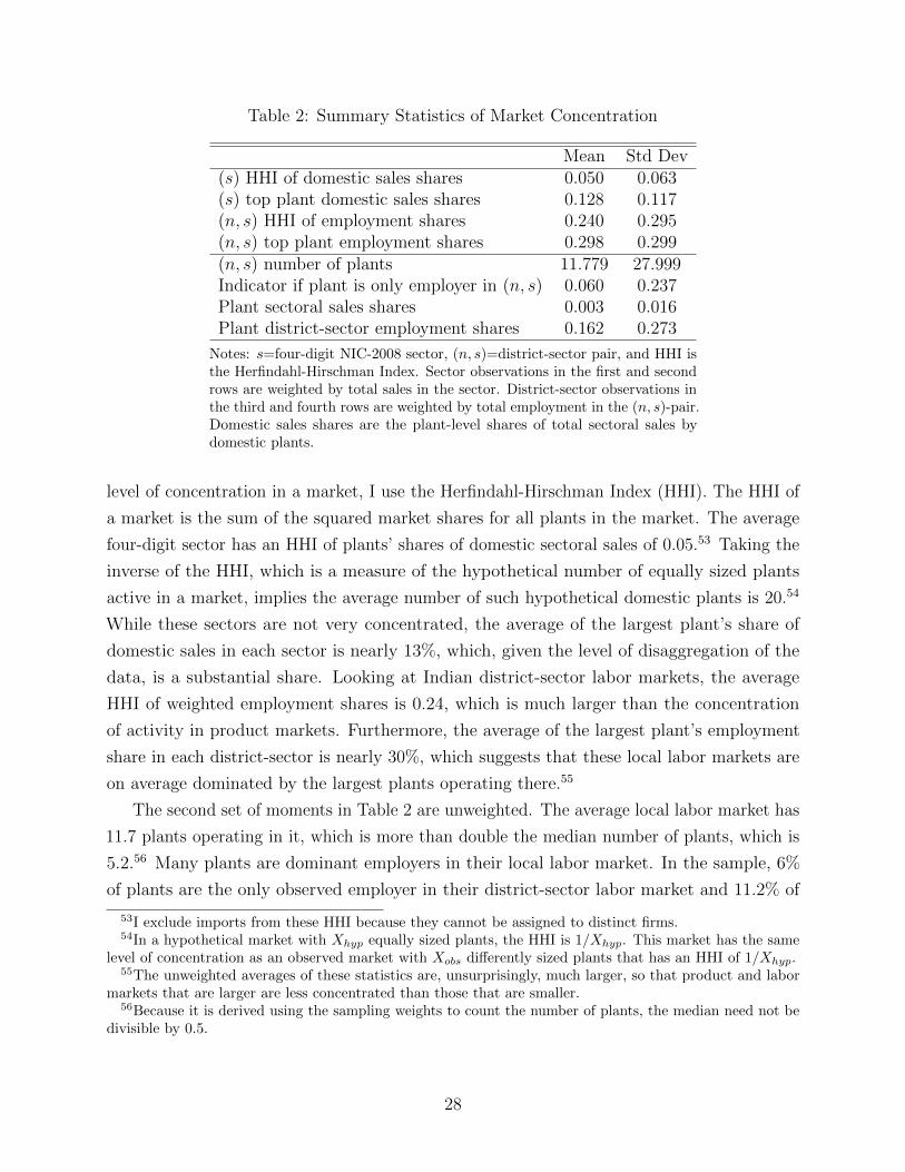
Table 2: Summary Statistics of Market Concentration

Mean Std Dev(s) HHI of domestic sales shares 0.050 0.063(s) top plant domestic sales shares 0.128 0.117(n, s) HHI of employment shares 0.240 0.295(n, s) top plant employment shares 0.298 0.299(n, s) number of plants 11.779 27.999Indicator if plant is only employer in (n, s) 0.060 0.237Plant sectoral sales shares 0.003 0.016Plant district-sector employment shares 0.162 0.273

Notes: s=four-digit NIC-2008 sector, (n, s)=district-sector pair, and HHI isthe Herfindahl-Hirschman Index. Sector observations in the first and secondrows are weighted by total sales in the sector. District-sector observations inthe third and fourth rows are weighted by total employment in the (n, s)-pair.Domestic sales shares are the plant-level shares of total sectoral sales bydomestic plants.

level of concentration in a market, I use the Herfindahl-Hirschman Index (HHI). The HHI of

a market is the sum of the squared market shares for all plants in the market. The average

four-digit sector has an HHI of plants’ shares of domestic sectoral sales of 0.05.53 Taking the

inverse of the HHI, which is a measure of the hypothetical number of equally sized plants

active in a market, implies the average number of such hypothetical domestic plants is 20.54

While these sectors are not very concentrated, the average of the largest plant’s share of

domestic sales in each sector is nearly 13%, which, given the level of disaggregation of the

data, is a substantial share. Looking at Indian district-sector labor markets, the average

HHI of weighted employment shares is 0.24, which is much larger than the concentration

of activity in product markets. Furthermore, the average of the largest plant’s employment

share in each district-sector is nearly 30%, which suggests that these local labor markets are

on average dominated by the largest plants operating there.55

The second set of moments in Table 2 are unweighted. The average local labor market has

11.7 plants operating in it, which is more than double the median number of plants, which is

5.2.56 Many plants are dominant employers in their local labor market. In the sample, 6%

of plants are the only observed employer in their district-sector labor market and 11.2% of

53I exclude imports from these HHI because they cannot be assigned to distinct firms.54In a hypothetical market with Xhyp equally sized plants, the HHI is 1/Xhyp. This market has the same

level of concentration as an observed market with Xobs differently sized plants that has an HHI of 1/Xhyp.55The unweighted averages of these statistics are, unsurprisingly, much larger, so that product and labor

markets that are larger are less concentrated than those that are smaller.56Because it is derived using the sampling weights to count the number of plants, the median need not be

divisible by 0.5.

28

plants have a labor market share larger than 50%.57 The average plant is small relative to

the size of its sector, with a sales share of just 0.3%. In contrast, the average plant is large

relative to the size of its local labor market, with an employment share of 16.2%. Together,

these observations imply that firm sizes in the Indian data are heavily skewed and that many

local labor markets are dominated by a small number of large employers.

4.2 Estimated and Fitted Parameters

The key model determinants of the importance of market power are the product demand and

labor supply elasticity parameters, the dispersion of firm productivities, and the exogenous

number of competitors in each local labor market. Following Gaubert and Itskhoki (2018), I

set the across-sector elasticity of substitution, θ, equal to one, which implies the outer nest of

preferences in equation (7) is Cobb-Douglas, and then use the model to estimate γ, α, and

β.58 Using the estimated values for the remaining elasticity parameters and data on firms’

product and labor market shares, I calculate the model-implied firm productivities and fit

them to a log-normal distribution to estimate a dispersion parameter for firm productivities.

Finally, I allow the number of competitors in each local labor market to be heterogeneous

and target the median number of employers in the ASI data.

When firms have market power in product and labor markets, the share of a firm’s

revenues that are paid to labor depends on their markups and markdowns. In terms of the

model, this labor share of revenues for a Home firm can be written as

wHn,s(ω)`Hn,s(ω)

rn,s(ω)=

rHn,s(ω)/rn,s(ω)

µHn,s(ω)/µLn,s(ω)+r∗Hn,s(ω)/rn,s(ω)

µ∗Hn,s(ω)/µLn,s(ω), (30)

where rn,s(ω) is total firm revenues, rHn,s(ω) is sales in Home, and r∗Hn,s(ω) is sales in Foreign.

All else being equal, an increase in either markup or a decrease in the markdown leads to a

smaller labor share of revenues.

Parameters γ, α, and β are estimated using equation (30) and data on total labor costs,

`cHn,s(ω) = wHn,s(ω)`Hn,s(ω), value added, vaHn,s(ω), and market shares.59 Domestic product

57Because the ASI samples a subset of employers with between 10 and 100 employees and does not samplefrom smaller employers, in reality there may be a smaller percentage of plants that are monopsonists.

58I assume θ = 1 because of the level of aggregation in the data, which, as noted in the previous subsection,implies firms have small product market shares on average. In the counterfactuals below, I assume that eachsector has an identical Cobb-Douglas weight in workers’ preferences.

59This estimation procedure is also used to recover elasticity parameters in Edmond et al. (2015) andKikkawa et al. (2018). To account for material and energy inputs, I use value added instead of sales revenue.These are the same in the model with labor as the only input. Value added is calculated following theguidelines in the ASI documentation as the difference between the total value of output and total inputexpenditures.

29

market shares SHn,s(ω) and labor market shares SLn,s(ω) can be calculated for Indian plants

using the ASI and import data. Because market shares in export markets are unobserved, I

use data for the subsample of plants that do not export and for whom rHn,s(ω) = rn,s(ω).60 The

model implies that the difference between the observed firm-level labor share of value added

and the firm-level distortion dHn,s(ω) defined in equation (26) is equal to zero for non-exporters.

I estimate the elasticity parameters by solving

minγ,α,β

∑s

∑n

∑ω

(`cHn,s(ω)

vaHn,s(ω)− dHn,s(ω)

)2

(31)

using non-linear least squares, where I assume that eHn,s(ω) =`cHn,s(ω)

vaHn,s(ω)− dHn,s(ω) represents a

mean-zero i.i.d. measurement error.

The parameter estimates and implied average elasticities are given in Table 3. Column (1)

shows the parameter estimates under the baseline specification in which θ = 1 and the labor

market shares are measured in terms of shares of mandays worked by all employees at each

plant. The estimate of γ, the within-sector elasticity of substitution, is 1.999, which implies

that γ > θ and therefore firms that are larger sellers within national sectoral product markets

face more inelastic product demand and charge higher markups over their marginal costs.61

The point estimates of the labor supply elasticity parameters are also consistent with the

model assumption that β > α. This implies that workers view jobs from the same local labor

market as closer substitutes for one another than jobs from different local labor markets and

that larger employers within a local labor market face more inelastic labor supply and offer

lower wage markdowns than do smaller employers.

The labor supply elasticity parameters are estimated with low precision. This imprecision

originates from the weak correlation observed in the data between plants’ shares of employment

in their local labor market and their labor shares of value added.62 Nevertheless, this

correlation is negative, which suggests that the assumption that β > α is correct. I conduct

simulated comparative statics in Section 5 for alternative parameter values to evaluate how

the results from the counterfactual experiments are sensitive to these parameters.

Using the parameter estimates, the model implies that the average firm-level labor supply

60Exporting plants account for 9.56% of observations, 14.93% of aggregate domestic sales, and 20.65% oftotal employment among plants that satisfy the sample selection criteria outlined in Appendix B.

61These estimated parameters imply that plants charge very high markups. The average labor share ofvalue added in the estimation sample is 43.64%. Through the lens of the model, this implies that plants havea high amount of market power on average. Because variation in these labor shares of value added is morehighly correlated with variation in product market shares than with variation in labor market shares, theestimated γ is quite low.

62This correlation is −0.032. In part, this is due to aggregation issues such as defining local labor marketsat the district-sector level for plants in every sector.

30

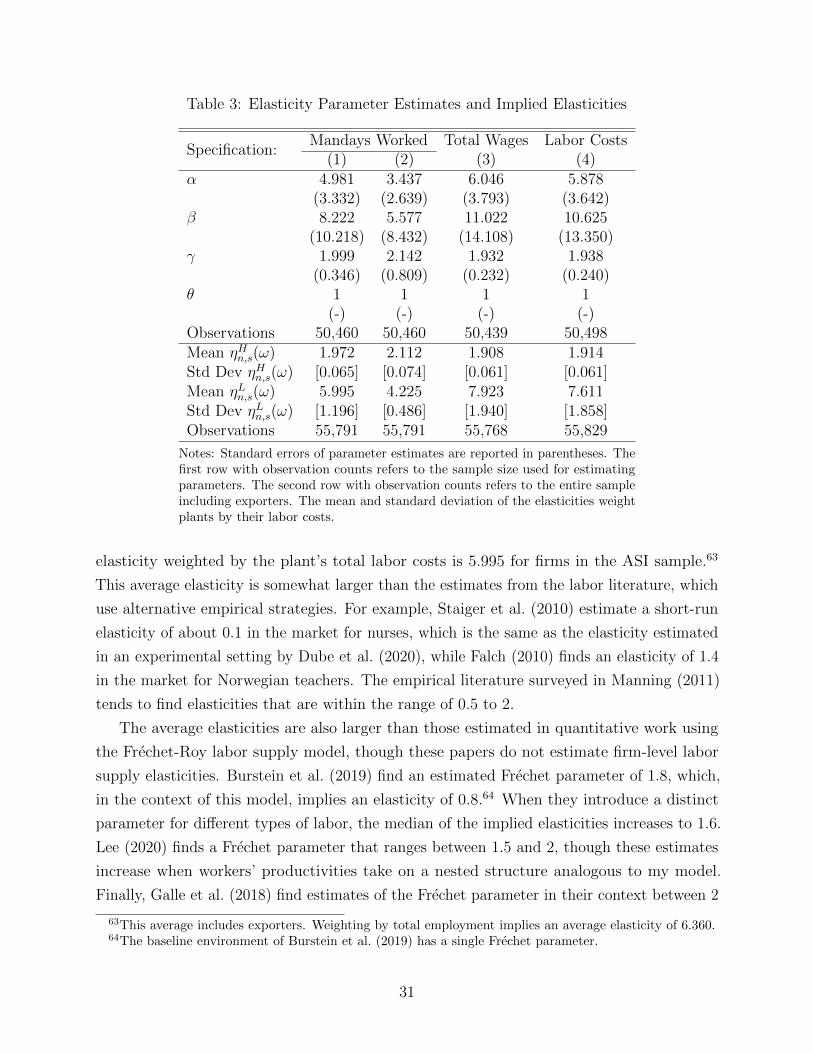
Table 3: Elasticity Parameter Estimates and Implied Elasticities

Specification:Mandays Worked Total Wages Labor Costs

(1) (2) (3) (4)α 4.981 3.437 6.046 5.878

(3.332) (2.639) (3.793) (3.642)β 8.222 5.577 11.022 10.625

(10.218) (8.432) (14.108) (13.350)γ 1.999 2.142 1.932 1.938

(0.346) (0.809) (0.232) (0.240)θ 1 1 1 1

(-) (-) (-) (-)Observations 50,460 50,460 50,439 50,498Mean ηHn,s(ω) 1.972 2.112 1.908 1.914Std Dev ηHn,s(ω) [0.065] [0.074] [0.061] [0.061]Mean ηLn,s(ω) 5.995 4.225 7.923 7.611Std Dev ηLn,s(ω) [1.196] [0.486] [1.940] [1.858]Observations 55,791 55,791 55,768 55,829

Notes: Standard errors of parameter estimates are reported in parentheses. Thefirst row with observation counts refers to the sample size used for estimatingparameters. The second row with observation counts refers to the entire sampleincluding exporters. The mean and standard deviation of the elasticities weightplants by their labor costs.

elasticity weighted by the plant’s total labor costs is 5.995 for firms in the ASI sample.63

This average elasticity is somewhat larger than the estimates from the labor literature, which

use alternative empirical strategies. For example, Staiger et al. (2010) estimate a short-run

elasticity of about 0.1 in the market for nurses, which is the same as the elasticity estimated

in an experimental setting by Dube et al. (2020), while Falch (2010) finds an elasticity of 1.4

in the market for Norwegian teachers. The empirical literature surveyed in Manning (2011)

tends to find elasticities that are within the range of 0.5 to 2.

The average elasticities are also larger than those estimated in quantitative work using

the Frechet-Roy labor supply model, though these papers do not estimate firm-level labor

supply elasticities. Burstein et al. (2019) find an estimated Frechet parameter of 1.8, which,

in the context of this model, implies an elasticity of 0.8.64 When they introduce a distinct

parameter for different types of labor, the median of the implied elasticities increases to 1.6.

Lee (2020) finds a Frechet parameter that ranges between 1.5 and 2, though these estimates

increase when workers’ productivities take on a nested structure analogous to my model.

Finally, Galle et al. (2018) find estimates of the Frechet parameter in their context between 2

63This average includes exporters. Weighting by total employment implies an average elasticity of 6.360.64The baseline environment of Burstein et al. (2019) has a single Frechet parameter.

31

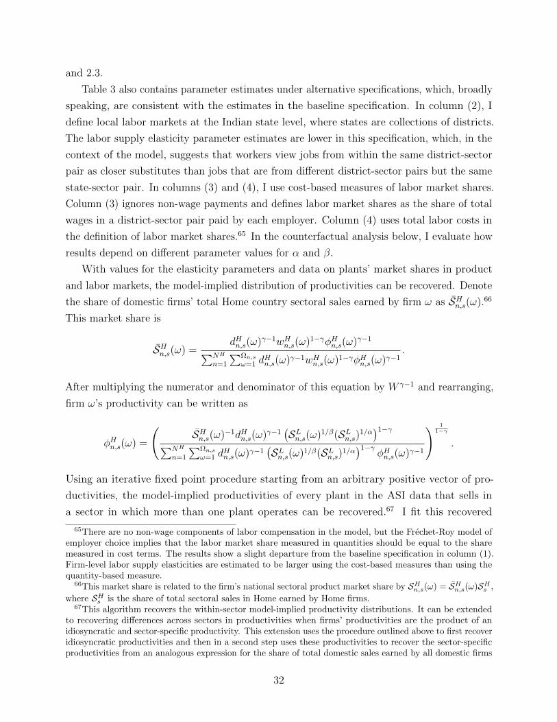
and 2.3.

Table 3 also contains parameter estimates under alternative specifications, which, broadly

speaking, are consistent with the estimates in the baseline specification. In column (2), I

define local labor markets at the Indian state level, where states are collections of districts.

The labor supply elasticity parameter estimates are lower in this specification, which, in the

context of the model, suggests that workers view jobs from within the same district-sector

pair as closer substitutes than jobs that are from different district-sector pairs but the same

state-sector pair. In columns (3) and (4), I use cost-based measures of labor market shares.

Column (3) ignores non-wage payments and defines labor market shares as the share of total

wages in a district-sector pair paid by each employer. Column (4) uses total labor costs in

the definition of labor market shares.65 In the counterfactual analysis below, I evaluate how

results depend on different parameter values for α and β.

With values for the elasticity parameters and data on plants’ market shares in product

and labor markets, the model-implied distribution of productivities can be recovered. Denote

the share of domestic firms’ total Home country sectoral sales earned by firm ω as SHn,s(ω).66

This market share is

SHn,s(ω) =dHn,s(ω)γ−1wHn,s(ω)1−γφHn,s(ω)γ−1∑NH

n=1

∑Ωn,sω=1 d

Hn,s(ω)γ−1wHn,s(ω)1−γφHn,s(ω)γ−1

.

After multiplying the numerator and denominator of this equation by W γ−1 and rearranging,

firm ω’s productivity can be written as

φHn,s(ω) =

(SHn,s(ω)−1dHn,s(ω)γ−1

(SLn,s(ω)1/β(SLn,s)1/α

)1−γ∑NH

n=1

∑Ωn,sω=1 d

Hn,s(ω)γ−1

(SLn,s(ω)1/β(SLn,s)1/α

)1−γφHn,s(ω)γ−1

) 11−γ

.

Using an iterative fixed point procedure starting from an arbitrary positive vector of pro-

ductivities, the model-implied productivities of every plant in the ASI data that sells in

a sector in which more than one plant operates can be recovered.67 I fit this recovered

65There are no non-wage components of labor compensation in the model, but the Frechet-Roy model ofemployer choice implies that the labor market share measured in quantities should be equal to the sharemeasured in cost terms. The results show a slight departure from the baseline specification in column (1).Firm-level labor supply elasticities are estimated to be larger using the cost-based measures than using thequantity-based measure.

66This market share is related to the firm’s national sectoral product market share by SHn,s(ω) = SHn,s(ω)SHs ,

where SHs is the share of total sectoral sales in Home earned by Home firms.67This algorithm recovers the within-sector model-implied productivity distributions. It can be extended

to recovering differences across sectors in productivities when firms’ productivities are the product of anidiosyncratic and sector-specific productivity. This extension uses the procedure outlined above to first recoveridiosyncratic productivities and then in a second step uses these productivities to recover the sector-specificproductivities from an analogous expression for the share of total domestic sales earned by all domestic firms

32

Figure 1: Recovered Productivity Distribution Fit

Productivity

De

nsity

Recovered Productivity Distribution

Data

Fitted Distribution

Notes: Figure shows the recovered productivity distribution andthe fitted log-normal distribution.

productivity distribution to a log-normal productivity distribution, which implies that the

standard deviation of the log of firm productivities is 2.591. The fit of this distribution

relative to the model-implied distribution of productivities recovered from the data is shown

in Figure 1. The log-normal distribution underestimates the frequency of very large and very

small firms and overstimates the frequency of moderately large firms.68

Finally, I allow the number of potential firms operating in each location-sector pair labor

market to be randomly determined. In particular, the number of firms is drawn independently

from a geometric distribution parameterized to match the median number of plants in Indian

district-sector labor markets, which is 5.2 in the ASI data.69

4.3 Fixed Parameters

The remaining parameters are chosen to facilitate analysis of the counterfactual experiments

described in the next section. I assume that Home and Foreign are symmetric as in Assump-

tion 1 so that all parameters are the same for both countries and each firm in a country has

in a sector. As I do not leverage differences across sectors for my quantitative experiments, I assume thatthese sector-specific productivities are all equal to one. See Edmond et al. (2015) for an example of thistwo-step extension.

68This discrepancy is in part due to the sampling frame of the ASI, which samples the largest firms withprobability one and samples smaller firms with a smaller probability.

69The geometric distribution parameter is 0.125.

33

an identical counterpart located in an identical local labor market in the other country.

I normalize the labor endowment in each country to be LH = L∗F = 1. Due to the

computational costs of solving the system of pricing equations, I set the number of locations

to 10 and the number of sectors to 20 and discuss how the quantitative results are sensitive

to increasing the number of labor and product markets below. Each firm’s productivity is

drawn independently from a log-normal distribution with standard deviation 2.591.

I focus on intensive margin reallocation effects of trade and leave the extensive margins

of firm behavior exogenous. As a baseline, I allow every potentially active firm to employ

workers and sell to both countries. I evaluate the implications of allowing only a subset of

firms to export in Section 5.3.

5 Quantitative Analysis

Using the parameter values discussed in the previous section, I conduct counterfactual

experiments to evaluate how accounting for firms’ oligopsony power in labor markets affects

equilibrium outcomes and the gains from trade.70 I first compare outcomes in autarky with

and without endogenous labor market power to show how heterogeneous distortions reallocate

market shares across employers and affect aggregate welfare and real wages. Next, I compare

the effects of opening to trade under different assumptions on firms’ labor market power to

quantify the extent to which gains from trade depend on these assumptions. I also discuss

how trade affects firm’s market power in product and labor markets. Finally, I show how the

effects of trade depend on the extensive margin of exporting by exogenously varying the set

of firms that export in free trade. For each set of counterfactual experiments, I discuss how

changes in the model parameters affect the outcomes of interest.

When comparing outcomes under oligopsony competition and perfect competition in labor

markets, I assume that the structure underlying workers’ employer choices is unchanged

so that firms continue to face upward sloping labor supply curves under either model of

competition.71 Under oligopsony, firms offer an endogenous wage markdown, while under

perfect competition wages are equal to the marginal revenue product of labor.

70I label these parameter values as the baseline case.71In other words, α and β are finite in both cases. An alternative experiment would be to assume that

all firms face perfectly elastic labor supply with α → ∞ and β → ∞. Under either assumption, firms donot mark down their wages. However, α influences aggregate labor productivity through the shifter λΓ, soincreasing α and β to cause firms to face perfectly elastic labor supply curves would change aggregate laborproductivity between the two experiments.

34

Figure 2: Variable Markups and Markdowns

1 2 3 4 5

Productivity Rank Within

Location-Sector Labor Market

2

2.5

3

3.5

4

4.5

Mark

up in A

uta

rky

Markups by Productivity Rank

Top Five Firms

Average Markup

1 2 3 4 5

Productivity Rank Within

Location-Sector Labor Market

0.79

0.8

0.81

0.82

0.83

0.84

0.85

0.86

0.87

0.88

Mark

dow

n in A

uta

rky

Markdowns by Productivity Rank

Top Five Firms

Average Markdown

Notes: Figure shows the markups and markdowns of the five most productive firms within each locallabor market and the size-weighted average within each rank. Each dot represents a single firm. Theleft panel shows the domestic markups and the right panel shows the markdowns.

5.1 Oligopsony, Firm-Level Distortions, and Welfare

As discussed in Section 2, when firms have endogenous market power and internalize the effects

of their prices and wages on their sectoral product market and local labor market competitors,

firm-level outcomes are distorted for two reasons: firms charge variable markups over their

marginal costs and offer variable markdowns on their wages. These variable distortions are

functions of firms’ sizes, which, in this model, depend on firms’ productivities and the set of

local labor market competitors. Figure 2 demonstrates the result in Proposition 1. It shows,

for a typical simulation, the markups and markdowns of the five most productive firms in

every local labor market as well as the average within each rank weighted by the size of the

firm.72 In every local labor market, the markup is decreasing and the markdown is increasing

in the productivity rank of the firm. Therefore, prices and wages are more distorted for more

productive firms than for less productive firms.

Figure 2 also demonstrates that in the calibrated model, variation in the markups and

markdowns across firms is largely constrained to the two or three most productive firms in each

local labor market. This is consistent with results in Gaubert and Itskhoki (2018). In part,

this reflects the large dispersion in plant-level productivities recovered from the Indian data.

The weighted average markup of the third most productive firm across location-sector pair

labor markets is 2.0316, which is only slightly larger than the CES markup of γγ−1

= 2.0015.

While there is more variation across local labor markets in the markdowns offered by firms,

72The weights for markups are sales while the weights for markdowns are labor costs.

35

the markdown under monopsonistic competition, β−1β

= 0.8784, is only slightly larger than

the weighted average markdown of the third and fourth most productive firms, which are

0.8725 and 0.8748, respectively.

The finding that the most productive firms within a local labor market offer lower wage

markdowns compared to less productive firms has two important implications for the effects

of oligopsony competition on firm-level outcomes. First, oligopsony power compresses the

distribution of wages per effective worker across firms within a local labor market. Second,

the most productive firms are too small compared to their local labor market competitors

relative to a counterfactual environment in which firms do not exercise labor market power.

Oligopsony competition causes a reduction in between-firm inequality of wages per effective

worker relative to perfect competition in labor markets because larger firms offer lower

markdowns.73 Under perfect competition, firms continue to face finitely elastic labor supply

curves. Therefore, there is still dispersion of wages per effective worker across firms under

perfect competition because heterogeneity in firm productivity implies firms have different

labor demand curves and offer different equilibrium wages.74 Because, under oligopsony

competition, the most productive firms offer lower wage markdowns, their wages are closer

to what their competitors offer than they would be without variable markdowns. When

markdown distortions are eliminated, the most productive firms increase their wages by more

than do less productive firms, as shown in Figure 3. This figure shows the ratio of real

wages per effective worker with perfect competition relative to oligopsony for the five most

productive firms in every local labor market as well as the weighted average across markets

within each rank.75 The most productive firms would also have the largest wage increases

when moving from an environment with oligopsony and variable markdowns to one with

monopsonistic competition and constant markdowns.

As a corollary to these effects of oligopsony on firm-level wages per effective worker,

firms’ sizes are distorted within local labor markets. Because the most productive firm in

a local labor market charges a higher markup and offers a lower markdown, they have a

larger distortion in their output supplied and labor demanded than do less productive firms.

The result of removing these distortions, which is displayed in Figure 4 for the five most

productive firms in every local labor market along with the cost-weighted average of these

ratios, is that the most productive firm in each market always increases in size relative to its

73There is no inequality in wages per employed worker because, from equations (5) and (6), these are equalto λΓW for all firms.

74If firms instead face perfectly elastic labor supply curves (e.g., if β →∞), every firm within a local labormarket offers the same wage per effective worker.

75Weights are labor costs under oligopsony. Within every local labor market, more productive firms increasetheir wage offer by more than do less productive firms. All firms increase their wage offer when oligopsonycompetition is eliminated because firms compete more intensely for labor.

36

Figure 3: Oligopsony and Between-Firm Inequality

1 2 3 4 5

Productivity Rank Within

Location-Sector Labor Market

1.165

1.17

1.175

1.18

1.185

1.19

1.195

1.2

1.205

1.21

Ratio o

f R

eal W

age

Perf

ect C

om

petition v

s O

ligopsony

Wage Increase By Rank

Top Five Firms

Average Ratio

Notes: Figure shows the ratio of real wages under perfect com-petition and oligopsony for the five most productive firms withineach local labor market and the cost-weighted average withineach rank. Each dot represents a single firm.

local competitors.

While this is true for the most productive firm in a local labor market, this need not be

the case for less productive firms. Figure 4 shows that almost all firms that are not the most

productive in their local labor market lose labor market share when oligopsony distortions

are eliminated, which is then reallocated to the most productive firms.76

Because the most productive firms within a local labor market are too small relative to

the less productive firms under oligopsony competition, aggregate welfare is smaller than it

would be with perfectly competitive labor markets. However, the calibrated model suggests

that these welfare losses are small. Aggregate real income is 0.35% smaller under oligopsony

than under perfect competition.77 While these welfare losses from oligopsony are small, the

composition of real income is very different in the two models. With oligopsony, aggregate

real wage income is only 84.48% of its level under perfect competition, while aggregate real

dividend income is 11.47% higher with oligopsony. The direction of divergence between the

two models in these results is unsurprising, since with more scope for exercising market power

firms should earn more profits holding the extensive margins of firm activity fixed. In an

alternative setting in which dividend income was distributed unequally to different workers,

76Furthermore, within a local labor market these ratios are strictly decreasing in the productivity rank ofthe firm.

77This comparison, and all comparisons in this subsection, assumes each country is in autarky. Furthermore,oligopoly competition in product markets is maintained in all counterfactuals.

37

Figure 4: Firm Size Distortions Within Labor Markets

1 2 3 4 5

Productivity Rank Within

Location-Sector Labor Market

0.84

0.86

0.88

0.9

0.92

0.94

0.96

0.98

1

1.02

1.04

Ratios o

f S

hare

s o

f Labor

Perf

ect C

om

petition / O

ligopsony

Change in relative employment

Perfect Competition vs. Oligopsony

Average Ratio

Notes: Figure shows the ratio of employment under perfectcompetition and oligopsony for the five most productive firmswithin each local labor market and the cost-weighted averagewithin each rank. Each dot represents a single firm.

accounting for endogenous labor market power would introduce additional inequality across

workers.

The finding that the welfare effects induced by firms’ variable markdowns are small does

not depend on the parameter values used for the labor supply elasticities. In Table 4, I show

the percentage change of welfare under oligopsony competition in labor markets relative to

perfect competition for a range of different labor supply elasticity parameters, all of which

imply only small welfare effects.78 As long as α 6= β, firms offer variable markdowns and

therefore firms’ sizes are distorted within local labor markets. Table 4 demonstrates the

general pattern that the larger is the gap between α and β, the larger is the welfare change

due to oligopsony.79 When α and β are larger, firms face more elastic labor supply curves

and offer larger markdowns to their workers. When both parameters increase proportionally,

the welfare effects of variable markdowns become smaller because variation across firms in

markdowns decreases, and hence the entries in the top left of Table 4 are in general larger in

78I do not recalibrate the distribution of productivity under these alternative elasticity parameters, so theseare comparative static experiments.

79When α > β, large firms offer larger markdowns than small firms and are therefore larger than theywould be relative to a constant markdown environment. Using the terminology of Dhingra and Morrow(2019), in this situation private and social incentives can be misaligned depending on the relative magnitudesof the product demand and labor supply elasticity parameters. When α and β are smaller, the relativevariation in markdowns across firms is larger and these incentives are more likely to be misaligned.

38

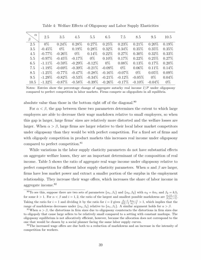
Table 4: Welfare Effects of Oligopsony and Labor Supply Elasticities

βα

2.5 3.5 4.5 5.5 6.5 7.5 8.5 9.5 10.5

2.5 0% 0.24% 0.28% 0.27% 0.25% 0.23% 0.21% 0.20% 0.19%3.5 -0.45% 0% 0.19% 0.28% 0.32% 0.34% 0.35% 0.35% 0.35%4.5 -0.77% -0.26% 0% 0.14% 0.22% 0.27% 0.30% 0.32% 0.33%5.5 -0.97% -0.45% -0.17% 0% 0.10% 0.17% 0.22% 0.25% 0.27%6.5 -1.11% -0.59% -0.29% -0.12% 0% 0.08% 0.13% 0.17% 0.20%7.5 -1.19% -0.69% -0.39% -0.21% -0.09% 0% 0.06% 0.11% 0.14%8.5 -1.25% -0.77% -0.47% -0.28% -0.16% -0.07% 0% 0.05% 0.09%9.5 -1.29% -0.82% -0.53% -0.34% -0.21% -0.12% -0.05% 0% 0.04%10.5 -1.32% -0.87% -0.58% -0.39% -0.26% -0.17% -0.10% -0.04% 0%

Notes: Entries show the percentage change of aggregate autarky real income I/P under oligopsonycompared to perfect competition in labor markets. Firms compete as oligopolists in all equilibria.

absolute value than those in the bottom right off of the diagonal.80

For α < β, the gap between these two parameters determines the extent to which large

employers are able to decrease their wage markdown relative to small employers, so when

this gap is larger, large firms’ sizes are relatively more distorted and the welfare losses are

larger. When α > β, large firms are larger relative to their local labor market competitors

under oligopsony than they would be with perfect competition. For a fixed set of firms and

with oligopoly competition in product markets this increases real income under oligopsony

compared to perfect competition.81

While variations in the labor supply elasticity parameters do not have substantial effects

on aggregate welfare losses, they are an important determinant of the composition of real

income. Table 5 shows the ratio of aggregate real wage income under oligopsony relative to

perfect competition for different labor supply elasticity parameters. When α and β are larger,

firms have less market power and extract a smaller portion of the surplus in the employment

relationship. They increase their wage offers, which increases the share of labor income in

aggregate income.82

80To see this, suppose there are two sets of parameters α1, β1 and α2, β2 with α2 = kα1 and β2 = kβ1

for some k > 1. For α < β and i = 1, 2, the ratio of the largest and smallest possible markdowns are αi(βi−1)βi(αi−1) .

Taking the ratio for i = 1 and dividing it by the ratio for i = 2 gives β1−1kβ1−1

kα1−1α1−1 > 1, which implies that the

range of markdowns decreases under α2, β2 relative to α1, β1. A similar argument holds for α > β.81When α > β, the distortions in firm sizes due to oligopsony counteracts the distortions in firm sizes due

to oligopoly that cause large sellers to be relatively small compared to a setting with constant markups. Theoligopsony equilibrium is not allocatively efficient, however, because the allocation does not correspond to theone that would be chosen by a social planner facing the same labor supply curves.

82The increased wage offers are due both to a reduction of markdowns and an increase in the intensity ofcompetition for workers.

39

Table 5: Oligopsony, Labor Supply Elasticities, and Aggregate Real Wages

βα

2.5 3.5 4.5 5.5 6.5 7.5 8.5 9.5 10.5

2.5 60.0% 65.4% 69.1% 71.8% 73.9% 75.6% 77.0% 78.2% 79.2%3.5 66.9% 71.4% 74.5% 76.8% 78.6% 80.0% 81.2% 82.2% 83.1%4.5 71.1% 75.1% 77.8% 79.8% 81.4% 82.6% 83.7% 84.6% 85.3%5.5 74.0% 77.6% 80.0% 81.8% 83.2% 84.4% 85.3% 86.1% 86.8%6.5 76.2% 79.4% 81.7% 83.3% 84.6% 85.7% 86.5% 87.3% 87.9%7.5 77.9% 80.9% 82.9% 84.5% 85.7% 86.7% 87.5% 88.2% 88.7%8.5 79.3% 82.1% 84.0% 85.4% 86.6% 87.5% 88.2% 88.9% 89.4%9.5 80.4% 83.1% 84.9% 86.2% 87.3% 88.2% 88.9% 89.5% 90.0%10.5 81.4% 83.9% 85.6% 86.9% 87.9% 88.7% 89.4% 90.0% 90.5%

Notes: Entries show the ratio of aggregate autarky real wage W/P under oligopsony relative toperfect competition in labor markets. Firms compete as oligopolists in all equilibria.

Aggregate welfare losses due to endogenous labor market power are also quite insensitive

to changes in the other model parameters, as shown in Table 6. When γ increases, goods

from the same sector become closer substitutes for one another, which reduces the market

power that firms have in product markets. As a result, market shares in product markets

shift towards firms that charge lower prices, so the extent of misallocation in the baseline

oligopsony equilibrium decreases. However, as γ increases, imperfect competition in labor

markets becomes a more important determinant of the composition of real income. Because

the most productive firms gain market share in product markets, they also gain market share

in labor markets, which allows them to offer lower wage markdowns.

Table 6 also shows the effects of changing the market environment that firms face and

the dispersion of firm productivities. When the location dimension of the model is removed

and all firms in a sector compete directly with each other within the same labor market,

welfare losses due to oligopsony are reduced. Firms have smaller labor market shares, so their

wage offers and sizes are less distorted compared to the equilibrium with perfect competition

in labor markets. The finding of small welfare losses does not depend on the number of

locations in a sector or the number of sectors.83 The magnitude of the welfare losses depends

on the dispersion of firm productivity draws. When the standard deviation of the log-normal

distribution from which they are drawn is halved, firms are on average more similar to one

another. This reduces the dispersion of market shares in both product and labor markets

across firms as well as the dispersion of market power. As a result, welfare losses are smaller.

If dispersion of productivities is removed entirely, as is the case in Heiland and Kohler (2018),

83I simulate the model with 20 potential local labor markets in each sector and with 40 sectors (and 10potential local labor markets per sector). This increases the number of total firms in operation, but hasnegligible impacts on welfare losses or the composition of real income.

40

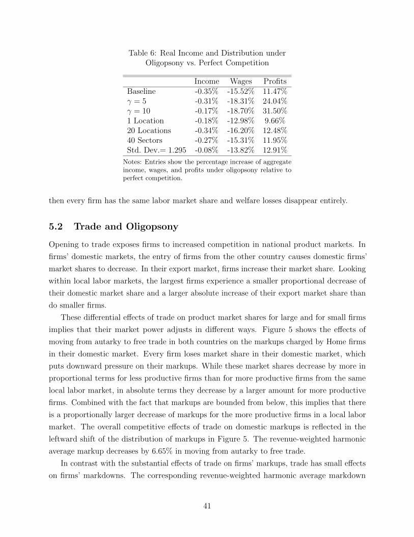
Table 6: Real Income and Distribution underOligopsony vs. Perfect Competition

Income Wages ProfitsBaseline -0.35% -15.52% 11.47%γ = 5 -0.31% -18.31% 24.04%γ = 10 -0.17% -18.70% 31.50%1 Location -0.18% -12.98% 9.66%20 Locations -0.34% -16.20% 12.48%40 Sectors -0.27% -15.31% 11.95%Std. Dev.= 1.295 -0.08% -13.82% 12.91%

Notes: Entries show the percentage increase of aggregateincome, wages, and profits under oligopsony relative toperfect competition.

then every firm has the same labor market share and welfare losses disappear entirely.

5.2 Trade and Oligopsony

Opening to trade exposes firms to increased competition in national product markets. In

firms’ domestic markets, the entry of firms from the other country causes domestic firms’

market shares to decrease. In their export market, firms increase their market share. Looking

within local labor markets, the largest firms experience a smaller proportional decrease of

their domestic market share and a larger absolute increase of their export market share than

do smaller firms.

These differential effects of trade on product market shares for large and for small firms

implies that their market power adjusts in different ways. Figure 5 shows the effects of

moving from autarky to free trade in both countries on the markups charged by Home firms

in their domestic market. Every firm loses market share in their domestic market, which

puts downward pressure on their markups. While these market shares decrease by more in

proportional terms for less productive firms than for more productive firms from the same

local labor market, in absolute terms they decrease by a larger amount for more productive

firms. Combined with the fact that markups are bounded from below, this implies that there

is a proportionally larger decrease of markups for the more productive firms in a local labor

market. The overall competitive effects of trade on domestic markups is reflected in the

leftward shift of the distribution of markups in Figure 5. The revenue-weighted harmonic

average markup decreases by 6.65% in moving from autarky to free trade.

In contrast with the substantial effects of trade on firms’ markups, trade has small effects

on firms’ markdowns. The corresponding revenue-weighted harmonic average markdown

41

Figure 5: Trade and Markups

2 2.2 2.4 2.6 2.8

Markups in Autarky

2

2.2

2.4

2.6

2.8

Ma

rku

ps in

Fre

e T

rad

e

Competitive Effects of

Trade on Markups

2 2.02 2.04 2.06 2.08 2.1

Markup

De

nsity

Distribution of Markups

Autarky

Free Trade

Notes: Figure shows the effect of trade on markups. The left panel plots every Home firm’s domesticmarkup in autarky and free trade. Each dot represents a single firm. The right panel plots thedistributions of markups under autarky and free trade.

decreases by only 0.21%, which implies that firms’ labor market power increases only slightly

on average due to trade. These small effects can be seen at the firm level in Figure 6,

where, for most firms, the ratio of their markdown under free trade relative to autarky is

approximately one. This figure shows that firms that offer the lowest markdowns in autarky,

which are firms that are large employers within their local labor markets, are more likely to

decrease their markdown when the two countries open to trade than are firms that offer the

highest markdowns in autarky. This reflects a slight reallocation of labor market shares from

the least productive to the most productive firms in a local labor market.

The main cause for these reallocations is the change in relative markups across firms

within local labor markets. Because the largest firms experience a larger proportional decrease

in their domestic markup, relative domestic demand for their variety increases compared to

smaller firms in their local labor market. At the same time, these firms increase their export

market shares by a larger amount. In combination, these shifts in relative product demand

are transmitted into an increase in relative labor demand in the largest employers within a

local labor market. Therefore, the largest firms grow relative to the smallest firms.

These reallocations have the potential to affect the distribution of wages across firms both

in the aggregate and within local labor markets. Figure 7 shows how firms’ wages increase

when the countries open to trade. Because competition for workers increases as the most

productive firms in a sector expand, trade causes every firm to increase their wage offer.

However, because the effects of trade on labor market power are small, the increase in wages

has only slight effects on inequality across firms in relative terms. While the distribution of

42

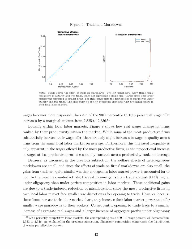
Figure 6: Trade and Markdowns

0.8 0.82 0.84 0.86 0.88

Markdowns in Autarky

0.8

0.82

0.84

0.86

0.88

Ma

rkd

ow

ns in

Fre

e T

rad

e

Competitive Effects of

Trade on Markdowns

0.8 0.82 0.84 0.86 0.88

Markdown

De

nsity

Distribution of Markdowns

Autarky

Free Trade

Notes: Figure shows the effect of trade on markdowns. The left panel plots every Home firm’smarkdown in autarky and free trade. Each dot represents a single firm. Larger firms offer lowermarkdowns compared to smaller firms. The right panel plots the distributions of markdowns underautarky and free trade. The mass point on the left represents employers that are monopsonists intheir local labor markets.

wages becomes more dispersed, the ratio of the 90th percentile to 10th percentile wage offer

increases by a marginal amount from 2.325 to 2.336.84

Looking within local labor markets, Figure 8 shows how real wages change for firms

ranked by their productivity within the market. While some of the most productive firms

substantially increase their wage offer, there are only slight increases in wage inequality across

firms from the same local labor market on average. Furthermore, this increased inequality is

only apparent in the wages offered by the most productive firms, as the proportional increase

in wages at less productive firms is essentially constant across productivity ranks on average.

Because, as discussed in the previous subsection, the welfare effects of heterogeneous

markdowns are small, and since the effects of trade on firms’ markdowns are also small, the

gains from trade are quite similar whether endogenous labor market power is accounted for or

not. In the baseline counterfactuals, the real income gains from trade are just 0.14% higher

under oligopsony than under perfect competition in labor markets. These additional gains

are due to a trade-induced reduction of misallocation, since the most productive firms in

each local labor market face smaller size distortions after opening to trade. However, because

these firms increase their labor market share, they increase their labor market power and offer

smaller wage markdowns to their workers. Consequently, opening to trade leads to a smaller

increase of aggregate real wages and a larger increase of aggregate profits under oligopsony

84With perfectly competitive labor markets, the corresponding ratio of 90-10 wage percentiles increases from2.333 to 2.346. As explained in the previous subsection, oligopsony competition compresses the distributionof wages per effective worker.

43

Figure 7: Trade and Real Wages

10 20 30 40 50 60

Real Wages in Autarky

10

20

30

40

50

60

Re

al W

ag

es in

Fre

e T

rad

eEffects of Trade on Real Wages

10 20 30 40 50 60

Real Wages

De

nsity

Distribution of Real Wages

Autarky

Free Trade

Notes: Figure shows the effect of trade on real wages. The left panel plots every Home firm’sreal wage in autarky and free trade. Each dot represents a single firm. The right panel plots thedistributions of real wages under autarky and free trade.

Figure 8: Trade and Between-Firm Inequality

1 2 3 4 5

Productivity Rank Within

Location-Sector Labor Market

2

2.05

2.1

2.15

2.2

2.25

2.3

2.35

2.4

2.45

Ratio o

f R

eal W

age

Fre

e T

rade v

s A

uta

rky

Wage Increase By Rank

Top Five Firms

Average Ratio

Notes: Figure shows the ratio of real wages under free tradeand autarky for the five most productive firms within each locallabor market and the cost-weighted average within each rank.Each dot represents a single firm.

44

Table 7: Gains from Trade and Labor Supply Elasticities: Oligopsony vs. PerfectCompetition

βα

2.5 3.5 4.5 5.5 6.5 7.5 8.5 9.5 10.5

2.5 0% -0.19% -0.31% -0.38% -0.41% -0.44% -0.45% -0.45% -0.45%3.5 0.16% 0% -0.11% -0.19% -0.24% -0.27% -0.29% -0.31% -0.32%4.5 0.24% 0.10% 0% -0.07% -0.13% -0.16% -0.19% -0.21% -0.23%5.5 0.28% 0.17% 0.07% 0% -0.05% -0.09% -0.12% -0.14% -0.16%6.5 0.30% 0.20% 0.12% 0.05% 0% -0.04% -0.07% -0.09% -0.11%7.5 0.31% 0.23% 0.15% 0.09% 0.04% 0% -0.03% -0.05% -0.07%8.5 0.32% 0.24% 0.17% 0.11% 0.07% 0.03% 0% -0.02% -0.04%9.5 0.32% 0.26% 0.19% 0.13% 0.09% 0.05% 0.02% 0% -0.02%10.5 0.32% 0.26% 0.20% 0.15% 0.11% 0.07% 0.04% 0.02% 0%

Notes: Entries show the percentage increase of real income I/P gains from trade under oligopsony relativeto perfect competition in labor markets. Gains from trade are measured as the ratio of free trade toautarky real income. Firms compete as oligopolists in all equilibria.

than under perfectly competitive labor markets. The baseline real wage gains from trade are

−0.36% smaller with oligopsony while the real profit growth is 1.92% higher.

These small effects on aggregate outcomes are robust to different labor supply elasticity

parameters. In Table 7, I demonstrate how the additional gains from trade change with

variation in these parameters. When labor supply is elastic for all firms (i.e., α and β are

large), the welfare effects of oligopsony are small because there is relatively little variation in

firms’ markdowns. Therefore, employers’ relative labor market shares are similar to what they

would be under perfect competition, so trade has similar effects on welfare under oligopsony

and perfect competition. Similarly, when the gap between the two elasticity parameters

is smaller, there is less variation in the markdowns across employers and the extent of

misallocation is smaller. However, as the gap between these parameters grows, the dispersion

of markdowns increases, which implies the most productive firms’ sizes are more distorted.

When α < β, the most productive firms are relatively small in the oligopsony equilibrium

in autarky. Trade reduces the extent of these size distortions by reallocating labor market

share towards those firms, so the gains from trade are larger under oligopsony and these

additional gains frome trade are increasing in the gap between α and β. In contrast, the

most productive firms are relatively large in the oligopsony equilibrium in autarky when

α > β. Trade increases the size distortions caused by oligopsony and the gains from trade

decrease. Intuitively, for a fixed set of firms the welfare benefits of increasing the relative size

of productive firms is smaller when they are relatively larger to begin with because consumers

view goods as imperfect substitutes.

In Table 8, I show the effect that different labor supply elasticity parameters have on the

45

Table 8: Gains from Trade, Labor Supply Elasticities, and Aggregate Wages: Oligopsonyvs. Perfect Competition

βα

2.5 3.5 4.5 5.5 6.5 7.5 8.5 9.5 10.5

2.5 0% 0.44% 0.65% 0.75% 0.81% 0.83% 0.84% 0.84% 0.83%3.5 -0.46% 0% 0.25% 0.40% 0.49% 0.54% 0.58% 0.60% 0.61%4.5 -0.73% -0.27% 0% 0.17% 0.27% 0.34% 0.39% 0.42% 0.45%5.5 -0.90% -0.45% -0.18% 0% 0.12% 0.20% 0.25% 0.30% 0.33%6.5 -1.02% -0.58% -0.30% -0.12% 0% 0.09% 0.15% 0.20% 0.23%7.5 -1.10% -0.67% -0.40% -0.22% -0.09% 0% 0.07% 0.12% 0.16%8.5 -1.16% -0.75% -0.48% -0.29% -0.16% -0.07% 0% 0.05% 0.10%9.5 -1.21% -0.80% -0.54% -0.35% -0.22% -0.13% -0.06% 0% 0.04%10.5 -1.24% -0.85% -0.59% -0.40% -0.27% -0.18% -0.10% -0.05% 0%

Notes: Entries show the percentage change of real wage W/P gains from trade under oligopsony relativeto perfect competition in labor markets. Real wage gains from trade are measured as the ratio of freetrade to autarky real wages. Firms compete as oligopolists in all equilibria.

real wage gains from trade under oligopsony compared to perfect competition. When α < β,

real wage growth is slower under oligopsony than it is under perfect competition because

the most productive firms gain additional market power in their labor markets due to the

reallocation of market share towards them. When labor supply is elastic, firms’ markdowns

are close to one, and workers’ benefits from the improvement in aggregate productivity are

similar under oligopsony and perfect competition. When α is relatively small compared to β,

the effect of trade-induced reallocations on the largest firms’ markdowns are larger, so the

real wage gains from trade are smaller with oligopsony. When α > β, trade causes the most

productive firms to lose market power in their labor markets as they grow in relative size.

Consequently, the real wage gains from trade are larger in this case.

Variation in the other model parameters has little effect on the additional gains from trade

under oligopsony, as shown in Table 9. In general, the effect of changing model parameters

on the gains follows the results presented in Table 6. When the losses due to misallocation

are larger, then trade leads to a larger increase in real income.85 The effects of trade on real

wage growth are also very similar with different parameter values compared to the baseline

equilibria.

Now consider the effects of taking a step away from the assumption of symmetric countries

as an additional trade shock. Suppose that aggregate productivity in Foreign increases such

85The additional gains when γ = 10 are smaller than when γ = 5 because the overall gains from trade aresubstantially smaller in the former case. The relative real wage gains are much more similar in the two cases.In both cases, aggregate dividend growth is much larger under oligopsony because without oligopsony, tradereduces aggregate profits in the symmetric country counterfactual.

46

Table 9: Gains from Trade: Oligopsony vs.Perfect Competition

Income Wages ProfitsBaseline 0.14% -0.36% 1.92%γ = 5 0.18% -0.74% 21.36%γ = 10 0.10% -0.86% 57.57%1 Location 0.03% -0.40% 1.62%20 Locations 0.12% -0.34% 1.73%40 Sectors 0.09% -0.33% 1.58%Std. Dev.= 1.295 0.02% -0.06% 0.40%

Entries show the percent increase of the gains from tradeand distribution under oligopsony compared to perfectcompetition in labor markets.

Table 10: Productivity Shocks andOligopsony vs. Perfect Competition

Income Wages Profits

Φ∗ = 1.112 0.003% -0.010% 0.049%Φ∗ = 2 0.015% -0.068% 0.316%

Notes: Entries show the effect of aggregate pro-ductivity shocks on real income, wages, and profitsunder oligopsony compared to perfect competition.

that each firm’s total factor productivity is multiplied by the factor Φ∗. Suppose, following the

median estimate in Hsieh and Ossa (2016) of China’s productivity growth over 1995 to 2007,

that Φ∗ = 1.112. Table 10 shows how this increase in Foreign productivity affects the free

trade equilibrium welfare in Home under oligopsony compared to perfect competition in labor

markets. An increase in Foreign productivity, like the effects of opening to trade, causes a

reallocation in Home product markets away from the least productive firms towards the most

productive firms, since the additional competition affects the least productive firms by more.

The results in this table show that there are additional gains when comparing oligospony

to perfect competition because these reallocations reduce the losses due to heterogeneous

variable markdowns. However, because the labor market power of the most productive firms

increases, the benefits of the improved productivity for Home workers’ wages is smaller under

oligopsony. When Φ∗ = 2, these effects are amplified, though the magnitude of these effects

are very small.

47

5.3 Extensive Margins

As a final counterfactual exercise, I consider the effects of the extensive margin of exporting

on the aggregate gains from trade. Instead of allowing every firm to export, suppose that only

a fraction of the most productive firms in each sector are able to export in free trade. When

only the most productive firms are able to export, there is a larger increase in their labor

market share when moving from autarky to free trade than in the baseline counterfactual of

the previous subsection. Both exporters and non-exporters face import competition in their

domestic product markets that reduces their market share there. However, non-exporters

lose additional market share in their local labor markets if there is an exporter there. As a

result, the most productive firms gain more labor market power than they would if every

firm were allowed to export.

In these experiments, I maintain Assumption 1 so that the set of exporters in each

country are identical. I consider the cases where, for each country, 10% and 20% of the

most productive firms in each sector export. I also introduce a symmetric fixed skilled labor

requirement of exporting paid by exporters in both countries and examine how variation

in these market access costs affects outcomes. Denote these labor requirements by fx for

Home firms. As the fixed labor requirement increases, the reallocation of labor towards the

exporters when opening to trade increases. However, because this labor used for fixed export

costs is not productive, less labor is available to produce output, which reduces aggregate

productivity.

Table 11 shows the quantitative effects of allowing only a fraction of the most productive

firms to export. Comparing the real income gains under oligopsony to perfect competition in

labor markets, real income growth under oligopsony is relatively larger when more firms are

able to export. The reason for this is because under oligopsony the additional reallocation in

labor markets towards the exporters causes them to offer lower markdowns and become more

distorted relative to perfect competition. Because they are more distorted, the relative sizes

of these firms are even smaller than what would prevail under perfect competition relative to

an equilibrium in which more firms exported. As a result, the additional gains from trade

due to oligopsony under the baseline case of the previous section are an upper bound on the

additional gains when the sets of producing and exporting firms are exogenous.

Increasing the fixed labor requirement for exporting causes both the real income and real

wage gains from trade to be more similar under oligopsony compared to perfect competition.

As fx increases, exporters demand more labor, which forces them to increase their wage

offer. Because exporters raise their wage offers, non-exporters also raise their wages due to

increased competition for workers. In addition, an increase in the fixed labor requirement of

exporting causes a reallocation of employment towards the more productive exporters and

48

Table 11: Gains from Trade, Exporting, andFixed Labor Requirement

10% Exporters 20% Exportersfx Income Wages Income Wages

0.000 0.052% -0.532% 0.074% -0.544%0.001 0.051% -0.520% 0.072% -0.498%0.002 0.050% -0.510% 0.070% -0.459%0.003 0.050% -0.500% 0.068% -0.425%0.004 0.049% -0.492% 0.067% -0.394%0.005 0.048% -0.486% 0.065% -0.366%0.006 0.047% -0.480% 0.063% -0.341%0.007 0.047% -0.475% 0.062% -0.317%0.008 0.046% -0.472% 0.060% -0.295%0.009 0.045% -0.469% 0.059% -0.274%0.010 0.044% -0.468% 0.057% -0.255%

Notes: Entries show percent increase of gains from tradeunder oligopsony compared to perfect competition in labormarkets for different exogenous amounts of exporters anddifferent fixed labor requirements, fx, for exporting. X%exporters means the X% most productive firms in eachsector are able to export.

away from less productive firms, which reduces the extent of misallocation due to variable

markdowns.

6 Conclusion

In this paper, I have developed a novel quantitative model in which heterogeneous firms

have endogenous market power in their national sectoral product markets and local labor

markets. I show how extending models of workers’ idiosyncratic choices that are becoming

increasingly used in the trade, labor, and macro literatures provides microfoundations for

firms’ endogenous labor market power. I apply the model to evaluate how trade affects firms’

market power in these markets and how accounting for endogenous labor market power affects

the gains from trade and the composition of these gains across workers’ wages and firms’

profits. This model provides a quantitatively tractable means of incorporating market power

of buyers in many input markets beyond labor markets. Moreover, while I study the effects

of a foreign trade shock, the model can be used to study other shocks at the sector or local

labor market level or to model labor market policies and institutions such as minimum wages

and unionization or policies designed to encourage export participation by small firms.

I quantify the importance of endogenous labor market power by estimating the model’s

49

key structural parameters with Indian plant-level data and sectoral import data. Using

the relationship between firm-level market power and factor payments, I provide a method

for recovering labor supply elasticities that is distinct from approaches used thus far in

the literature. This method can be used in other national contexts in both developed and

developing countries and outside the manufacturing industry to measure firms’ labor market

power. The Indian data support the view that firms that are larger sellers in their product

markets have more market power than smaller sellers, and firms that are larger employers in

their local labor markets have more market power than smaller employers.

I find that in the Indian context, the extent of firms’ labor market power is small, which

implies that there are only small welfare losses due to the misallocation of resources that is

caused by firms’ heterogeneous labor market power. Consequently, exposure to trade generates

only small additional welfare gains when comparing models with imperfect competition to

perfect competition in labor markets. However, the mechanism through which these additional

gains are realized is through a reallocation of market shares in local labor markets towards

the most productive firms within those markets, which increases the labor market power of

those firms. As a result, the distribution of the gains from trade is slightly shifted away from

workers’ wages towards firms’ profits when I account for endogenous labor market power.

This redistribution of the gains from trade is amplified when fewer firms can export.

The findings and model in this paper point to numerous interesting directions for future

research. For instance, because firms’ labor market power depends on the set of local

competitors they face, productive firms have an incentive to locate their plants and offices

in places where few other productive firms within their sector are operating. This divide

and conquer strategy of production location decisions does not factor into the present model

because firms’ locations are exogenous. Future research can investigate how the location

decisions of productive firms affects the market structure of local labor markets and outcomes

for both workers and firms. Additionally, extending the model to account for non-labor inputs

and costly trade across locations would allow for an evaluation of the tradeoff between firms’

proximity to their input suppliers and their ability to offer workers smaller wages in locations

and countries with less competitive labor markets.

Another important path for future research is to examine how market and bargaining

power on both sides of labor markets is affected by trade and in turn how this affects worker

and firm outcomes. Coordination by workers, as in, for example, unions, affects the share of

the surplus in employment relationships that is earned by workers. The model in this paper

predicts that large employers’ labor market power increases due to trade. A natural question

to ask is how inequality across workers that participate in unionized versus non-unionized

workplaces is influenced by variation in how trade affects competition across employers and

50

local labor markets. Furthermore, the model can be used to investigate coordination by

employers to reduce wages and policy interventions to prevent these practices.

51

References

Ahn, JaeBin and Alexander F McQuoid (2017) “Capacity Constrained Exporters: Identifying

Increasing Marginal Cost,” Economic Inquiry, Vol. 55, No. 3, pp. 1175–1191.

Almunia, Miguel, Pol Antras, David Lopez-Rodriguez, and Eduardo Morales (2018) “Venting

Out: Exports during a Domestic Slump,” working paper.

Antras, Pol, Teresa C Fort, and Felix Tintelnot (2017) “The Margins of Global Sourcing:

Theory and Evidence from US Firms,” American Economic Review, Vol. 107, No. 9, pp.

2514–64.

Arkolakis, Costas, Arnaud Costinot, Dave Donaldson, and Andres Rodrıguez-Clare (2019)

“The Elusive Pro-Competitive Effects of Trade,” The Review of Economic Studies, Vol. 86,

No. 1, pp. 46–80.

Arkolakis, Costas and Fabian Eckert (2017) “Combinatorial Discrete Choice,” working paper.

Ashenfelter, Orley C, Henry Farber, and Michael R Ransom (2010) “Labor Market Monop-

sony,” Journal of Labor Economics, Vol. 28, No. 2, pp. 203–210.

Atkeson, Andrew and Ariel Burstein (2008) “Pricing-to-Market, Trade Costs, and Interna-

tional Relative Prices,” American Economic Review, Vol. 98, No. 5, pp. 1998–2031.

Autor, David, David Dorn, Lawrence F Katz, Christina Patterson, and John Van Reenen

(2017) “Concentrating on the Fall of the Labor Share,” American Economic Review, Vol.

107, No. 5, pp. 180–85.

(2020) “The Fall of the Labor Share and the Rise of Superstar Firms,” The Quarterly

Journal of Economics, Vol. 135, No. 2, pp. 645–709.

Azar, Jose, Ioana Marinescu, and Marshall Steinbaum (2020a) “Labor Market Concentration,”

Journal of Human Resources, pp. 1218–9914R1.

Azar, Jose, Ioana Marinescu, Marshall Steinbaum, and Bledi Taska (2020b) “Concentration

in US Labor Markets: Evidence from Online Vacancy Data,” Labour Economics, Vol. 66.

Barkai, Simcha (2020) “Declining Labor and Capital Shares,” The Journal of Finance, Vol.

75, No. 5, pp. 2421–2463.

Barth, Erling, Alex Bryson, James C Davis, and Richard Freeman (2016) “It’s Where You

Work: Increases in the Dispersion of Earnings Across Establishments and Individuals in

the United States,” Journal of Labor Economics, Vol. 34, No. S2, pp. S67–S97.

52

Benmelech, Efraim, Nittai Bergman, and Hyunseob Kim (2020) “Strong Employers and

Weak Employees: How Does Employer Concentration Affect Wages?” Journal of Human

Resources, pp. 0119–10007R1.

Berger, David W, Kyle F Herkenhoff, and Simon Mongey (2019) “Labor Market Power,”

NBER Working Paper 25719, National Bureau of Economic Research.

Bernard, Andrew B, J Bradford Jensen, and Peter K Schott (2009) “Importers, Exporters,

and Multinationals: A Portrait of Firms in the U.S. that Trade Goods,” in Dunne, T J,

J B Jensen, and Roberts M eds. Producer Dynamics: New Evidence from Micro Data, pp.

513–552: University of Chicago Press.

Bhaskar, Venkataraman and Ted To (2003) “Oligopsony and the Distribution of Wages,”

European Economic Review, Vol. 47, No. 2, pp. 371–399.

Blum, Bernardo S, Sebastian Claro, and Ignatius J Horstmann (2013) “Occasional and

Perennial Exporters,” Journal of International Economics, Vol. 90, No. 1, pp. 65–74.

Brooks, Wyatt J, Joseph P Kaboski, Yao Amber Li, and Wei Qian (2019) “Exploitation of

Labor? Classical Monopsony Power and Labor’s Share,” NBER Working Paper 25660,

National Bureau of Economic Research.

Burstein, Ariel, Eduardo Morales, and Jonathan Vogel (2019) “Changes in Between-Group

Inequality: Computers, Occupations, and International Trade,” American Economic

Journal: Macroeconomics, Vol. 11, No. 2, pp. 348–400.

Card, David, Ana Rute Cardoso, Jorg Heining, and Patrick Kline (2018) “Firms and Labor

Market Inequality: Evidence and Some Theory,” Journal of Labor Economics, Vol. 36, No.

S1, pp. S13–S70.

Card, David, Jorg Heining, and Patrick Kline (2013) “Workplace Heterogeneity and the Rise

of West German Wage Inequality,” The Quarterly Journal of Economics, Vol. 128, No. 3,

pp. 967–1015.

CEA (2016a) “Benefits of Competition and Indicators of Market Power,” Council of Economic

Advisers Issue Brief, Council of Economic Advisers.

(2016b) “Labor Market Monopsony: Trends, Consequences, and Policy Responses,”

Council of Economic Advisers Issue Brief, Council of Economic Advisers.

De Loecker, Jan and Jan Eeckhout (2020) “Global Market Power,” working paper.

53

Dhingra, Swati and John Morrow (2019) “Monopolistic Competition and Optimum Product

Diversity Under Firm Heterogeneity,” Journal of Political Economy, Vol. 127, No. 1, pp.

196–232.

Dube, Arindrajit, Jeff Jacobs, Suresh Naidu, and Siddharth Suri (2020) “Monopsony in

Online Labor Markets,” American Economic Review: Insights, Vol. 2, No. 1, pp. 33–46.

Eaton, Jonathan and Samuel Kortum (2002) “Technology, Geography, and Trade,” Econo-

metrica, Vol. 70, No. 5, pp. 1741–1779.

Eaton, Jonathan, Samuel Kortum, and Sebastian Sotelo (2013) “International Trade: Linking

Micro and Macro,” in Advances in Economics and Econometrics: Tenth World Congress,

Vol. 2, pp. 329–370, Cambridge University Press.

Edmond, Chris, Virgiliu Midrigan, and Daniel Yi Xu (2015) “Competition, Markups, and

the Gains from International Trade,” American Economic Review, Vol. 105, No. 10, pp.

3183–3221.

(2018) “How Costly Are Markups?”Technical report, National Bureau of Economic

Research.

Elsby, Michael WL, Bart Hobijn, and Aysegul Sahin (2013) “The Decline of the US Labor

Share,” Brookings Papers on Economic Activity, Vol. 2013, No. 2, pp. 1–63.

Epifani, Paolo and Gino Gancia (2011) “Trade, Markup Heterogeneity and Misallocations,”

Journal of International Economics, Vol. 83, No. 1, pp. 1–13.

Falch, Torberg (2010) “The Elasticity of Labor Supply at the Establishment Level,” Journal

of Labor Economics, Vol. 28, No. 2, pp. 237–266.

Furman, Jason and Peter Orszag (2015) “A Firm-Level Perspective on the Role of Rents in

the Rise in Inequality,” working paper.

Galle, Simon, Andres Rodrıguez-Clare, and Moises Yi (2018) “Slicing the Pie: Quantifying

the Aggregate and Distributional Effects of Trade,” working paper.

Gaubert, Cecile and Oleg Itskhoki (2018) “Granular Comparative Advantage,” NBER

Working Paper 24807, National Bureau of Economic Research.

Grassi, Basile (2017) “IO in IO: Competition and Volatility in Input-Output Networks,”

working paper.

54

Heiland, Inga and Wilhelm Kohler (2018) “Heterogeneous Workers, Trade, and Migration,”

working paper.

Hsieh, Chang-Tai, Erik Hurst, Charles I Jones, and Peter J Klenow (2019) “The Allocation

of Talent and US Economic Growth,” Econometrica, Vol. 87, No. 5, pp. 1439–1474.

Hsieh, Chang-Tai and Peter J Klenow (2009) “Misallocation and Manufacturing TFP in

China and India,” The Quarterly Journal of Economics, Vol. 124, No. 4, pp. 1403–1448.

Hsieh, Chang-Tai and Ralph Ossa (2016) “A Global View of Productivity Growth in China,”

Journal of International Economics, Vol. 102, pp. 209–224.

Karabarbounis, Loukas and Brent Neiman (2013) “The Global Decline of the Labor Share,”

The Quarterly Journal of Economics, Vol. 129, No. 1, pp. 61–103.

(2019) “Accounting for Factorless Income,” NBER Macroeconomics Annual, Vol. 33,

No. 1, pp. 167–228.

Kikkawa, Ayuma Ken, Glenn Magerman, and Emmanuel Dhyne (2018) “Imperfect Competi-

tion and the Transmission of Shocks: The Network Matters,” working paper.

Lagakos, David and Michael E Waugh (2013) “Selection, Agriculture, and Cross-Country

Productivity Differences,” American Economic Review, Vol. 103, No. 2, pp. 948–80.

Lee, Eunhee (2020) “Trade, Inequality, and the Endogenous Sorting of Heterogeneous

Workers,” Journal of International Economics, p. 103310.

Liu, Yanping (2018) “Capital Adjustment Costs: Implications for Domestic and Export Sales

Dynamics,” working paper.

Manning, Alan (2011) “Imperfect Competition in the Labor Market,” in Card, David and

Orley Ashenfelter eds. Handbook of Labor Economics, Vol. 4, pp. 973–1041: Elsevier.

Melitz, Marc J (2003) “The Impact of Trade on Intra-Industry Reallocations and Aggregate

Industry Productivity,” Econometrica, Vol. 71, No. 6, pp. 1695–1725.

Melitz, Marc J and Stephen J Redding (2014) “Heterogeneous Firms and Trade,” in Gopinath,

Gita, Elhanan Helpman, and Kenneth Rogoff eds. Handbook of International Economics,

Vol. 4, pp. 1–54: Elsevier.

Melitz, Marc J and Daniel Trefler (2012) “Gains from Trade When Firms Matter,” Journal

of Economic Perspectives, Vol. 26, No. 2, pp. 91–118.

55

Morlacco, Monica (2019) “Market Power in Input Markets: Theory and Evidence from French

Manufacturing,” working paper.

Pavcnik, Nina (2002) “Trade Liberalization, Exit, and Productivity Improvements: Evidence

from Chilean Plants,” The Review of Economic Studies, Vol. 69, No. 1, pp. 245–276.

Peters, Michael (2020) “Heterogeneous Markups, Growth, and Endogenous Misallocation,”

Econometrica, Vol. 88, No. 5, pp. 2037–2073.

Ramondo, Natalia and Andres Rodrıguez-Clare (2013) “Trade, Multinational Production,

and the Gains from Openness,” Journal of Political Economy, Vol. 121, No. 2, pp. 273–322.

Restuccia, Diego and Richard Rogerson (2008) “Policy Distortions and Aggregate Productivity

with Heterogeneous Establishments,” Review of Economic Dynamics, Vol. 11, No. 4, pp.

707–720.

Rossi-Hansberg, Esteban, Pierre-Daniel Sarte, and Nicholas Trachter (2018) “Diverging Trends

in National and Local Concentration,”Technical report, National Bureau of Economic

Research.

Roy, Andrew Donald (1951) “Some Thoughts on the Distribution of Earnings,” Oxford

Economic Papers, Vol. 3, No. 2, pp. 135–146.

Soderbery, Anson (2014) “Market Size, Structure, and Access: Trade with Capacity Con-

straints,” European Economic Review, Vol. 70, pp. 276–298.

Song, Jae, David J Price, Fatih Guvenen, Nicholas Bloom, and Till Von Wachter (2019)

“Firming Up Inequality,” The Quarterly Journal of Economics, Vol. 134, No. 1, pp. 1–50.

Staiger, Douglas O, Joanne Spetz, and Ciaran S Phibbs (2010) “Is There Monopsony in the

Labor Market? Evidence from a Natural Experiment,” Journal of Labor Economics, Vol.

28, No. 2, pp. 211–236.

Suarez Serrato, Juan Carlos and Owen Zidar (2016) “Who Benefits from State Corporate Tax

Cuts? A Local Labor Markets Approach with Heterogeneous Firms,” American Economic

Review, Vol. 106, No. 9, pp. 2582–2624.

Thisse, Jacques-Francois and Eric Toulemonde (2015) “How Monopsonistic and Monopolistic

Competition Affects Wage Disparities?” working paper.

Traina, James (2018) “Is Aggregate Market Power Increasing? Production Trends Using

Financial Statements,” working paper.

56

Tsivanidis, Nick (2018) “The Aggregate and Distributional Effects of Urban Transit Infras-

tructure: Evidence from Bogota’s TransMilenio,” working paper.

Vannoorenberghe, Gonzague (2012) “Firm-Level Volatility and Exports,” Journal of Interna-

tional Economics, Vol. 86, No. 1, pp. 57–67.

57

A Derivation of Model Results

A.1 Labor Supply Curves

This appendix derives the firm-level labor supply curves in Home shown in Section 2.2. The

steps involved follow Lagakos and Waugh (2013) and Hsieh et al. (2019) and the derivation

of choice probabilities with multivariate Frechet distributed productivities in Ramondo and

Rodrıguez-Clare (2013). Use of the Frechet distribution in trade models was pioneered by

Eaton and Kortum (2002). Workers’ match-specific productivities are drawn from

G(ε(h)) = exp

(−∑NH

n=1

∫ 1

0

(∑ΩHn,s

ω=1εn,s(h, ω)−β)

α/β

ds

).

Let Gω(ε(h)) be the derivative of this distribution function with respect to the match-specific

productivity at employer ω in location-sector pair (n, s). This derivative is

Gω(ε(h)) = αεn,s(h, ω)−β−1

(∑ΩHn,s

ω′=1εn,s(h, ω

′)−β)α/β−1

G(ε(h)).

Evaluating this derivative at εn′,s′(h, ω′) =

wHn,s(ω)

wHn′,s′ (ω

′)εn,s(h, ω) for all ω′ in every (n′, s′)-pair

gives the probability that employer ω offers the highest nominal income to worker h of any

potential employer conditional on worker h having match-specific productivity εn,s(h, ω) with

that employer. This probability is given by

αεn,s(h, ω)−α−1G

(wHn,s(ω)

wHn′,s′(ω′)εn,s(h, ω)

)wHn,s(ω)β−αWn,s

α−β, (32)

where Wn,s is defined as in equation (3) and

G

(wHn,s(ω)

wHn′,s′(ω′)εn,s(h, ω)

):= exp

(−εn,s(h, ω)−αwHn,s(ω)−α

(∑NH

n′=1

∫ 1

0

Wn′,s′αds′

))

is the distribution function for match-specific productivities evaluated at εn′,s′(h, ω′) =

wHn,s(ω)

wHn′,s′ (ω

′)εn,s(h, ω) for all potential employers.

58

Notice that∫∞

0

(∂G

(wHn,s(ω)

wHn′,s′ (ω

′)εn,s(h, ω)

)/∂εn,s(h, ω)

)dεn,s(h, ω) = 1, and

∂G

(wHn,s(ω)

wHn′,s′ (ω

′)εn,s(h, ω)

)∂εn,s(h, ω)

= αεn,s(h, ω)−α−1G

(wHn,s(ω)

wHn′,s′(ω′)εn,s(h, ω)

)wHn,s(ω)−αWα,

where W =(∑NH

n=1

∫ 1

0Wn,s

αds)1/α

. Combining these observations, the probability that

worker h chooses employer ω, which is the integral of equation (32) over the range of possible

match-specific productivities, is given by(wHn,s(ω)

Wn,s

)β (Wn,s

W

)α. (33)

Since this probability is independent of the identity of the worker and all workers share

a common distribution from which match-specific productivities are drawn, this is the

probability that any worker chooses employer ω as given in the main text by equation (2).

Equivalently, because there is a continuum of workers, this probability is equal to the market

share of total employment at firm ω.

The average productivity of employer ω’s workers depends on the conditional distribution

of their productivities. Denote this conditional distribution by G(z;ω), where

G(z;ω) = Pr

[εn,s(h, ω) < z

∣∣∣∣∣ wHn,s(ω)

wHn′,s′(ω′)εn,s(h, ω) > εn′,s′(h, ω

′) ∀ω′, n′, s′]

=

Pr

[εn,s(h, ω) < z and

wHn,s(ω)

wHn′,s′ (ω

′)εn,s(h, ω) > εn′,s′(h, ω

′) ∀ω′, n′, s′]

Pr

[wHn,s(ω)

wHn′,s′ (ω

′)εn,s(h, ω) > εn′,s′(h, ω′) ∀ω′, n′, s′

] .

The denominator of this equation is just the unconditional choice probability in equation (33).

The numerator is the integral of equation (32) over εn,s(h, ω) from zero to z. Therefore, the

conditional distribution of ω’s workers’ productivities is

G(z;ω) = exp(−z−αwHn,s(ω)−αWα

).

Using this conditional distribution, the expected productivity of a given worker h at ω is

59

given by

E[z | h chooses ω] =

∫ ∞0

αz−αwHn,s(ω)−αWα exp(−z−αwHn,s(ω)−αWα

)dz

=W

wHn,s(ω)

∫ ∞0

x−1/α exp(−x)dx

=W

wHn,s(ω)Γ(1− 1/α), (34)

where the second equality uses the change of variables x = z−αwHn,s(ω)−αWα, and Γ(1− 1/α)

is the gamma function evaluated at 1− 1/α.

Because the probability that a worker chooses ω is independent across workers, effective

labor supply to the firm is the product of three terms: the probability that the firm is chosen,

given by equation (33); the expected productivity of a worker conditional on choosing the

firm, given by equation (34); and the number of workers, LH . This product is given by

equation (6) in the main text.

A.2 Proof of Proposition 1

Suppose that the two firms under comparison sell to both markets. The argument below

extends to either alternative case with the firms selling to only one of the product markets. For

the first statement of the proposition, suppose that φHn,s(ω) > φHn,s(ω′) but that the statement is

untrue. If yHn,s(ω) ≤ yHn,s(ω′), then `Hn,s(ω) ≤ `Hn,s(ω

′) since labor is the only input in production.

If instead wHn,s(ω) ≤ wHn,s(ω′), then `Hn,s(ω) ≤ `Hn,s(ω

′) because, from equation (6), relative

effective employment at any two firms from the same local labor market depends only on their

relative wage offers. Lastly, if µLn,s(ω) ≥ µLn,s(ω′), then SLn,s(ω) ≤ SLn,s(ω′) since differences in

markdowns depend on differences in employment shares. Therefore, if the statement is false,

it must be the case that SLn,s(ω) ≤ SLn,s(ω′). If ω′ hires more workers compared to ω, then it

must be true that wHn,s(ω) ≤ wHn,s(ω′) and µLn,s(ω) ≥ µLn,s(ω

′). Therefore,

wHn,s(ω′)

µLn,s(ω′)≥wHn,s(ω)

µLn,s(ω).

The ratio of the wage over the markdown is just the marginal effective hiring cost of the firm,

which, under profit maximization, implies that marginal revenue products of effective labor

in Home must satisfy

pHn,s(ω′)φHn,s(ω

′)

µHn,s(ω′)

≥pHn,s(ω)φHn,s(ω)

µHn,s(ω).

60

However, this inequality implies that marginal revenue in Home at ω′ must be larger than

marginal revenue at ω, since

pHn,s(ω′)/µHn,s(ω

′)

pHn,s(ω)/µHn,s(ω)≥φHn,s(ω)

φHn,s(ω′)> 1

by assumption. But if marginal revenue in Home is larger at ω′ than at ω, the same must

be true for marginal revenue in Foreign. Since marginal revenue is strictly decreasing in

the amount sold by firms, this implies that ω′ sells a smaller amount to both Home and

Foreign. If this is true, however, then ω′ must be producing a smaller amount than ω, or

yHn,s(ω) < yHn,s(ω′). Since labor is the only input in production, ω must hire more effective

labor, pay higher wages per efficiency unit, and offer a lower markdown. Therefore, the first

statement in the proposition must be true.

Now suppose the second statement of the proposition is untrue. If pHn,s(ω) ≥ pHn,s(ω′) and

p∗Hn,s(ω) ≥ p∗Hn,s(ω′), then, since demand curves are downward sloping, ω′ must sell more to

both national product markets than does ω. Were this the case, then ω′ must hire more

workers than ω since they produce a larger amount of output with a smaller total factor

productivity. But this has already been shown to be incompatible with the first statement of

the proposition, so this cannot be true.

Alternatively, the second statement could be false if the ranking of the two firms’ prices

are different in each national product market. Suppose that pHn,s(ω) < pHn,s(ω′) but that

p∗Hn,s(ω) ≥ p∗Hn,s(ω′). Since relative market shares and hence markups for these two firms

depend only on the relative prices, this implies that (pHn,s(ω)/µHn,s(ω)) < (pHn,s(ω′)/µHn,s(ω

′)) and

(p∗Hn,s(ω)/µ∗Hn,s(ω)) ≥ (p∗Hn,s(ω′)/µ∗Hn,s(ω

′)). However, these two inequalities are not simultaneously

compatible with profit maximization, since they imply that for at least one of the firms the

marginal revenue of allocating a unit of output to Home is not equal to the marginal revenue

of allocating it to Foreign. Therefore, the second statement of the propsition must be true.

The assumption that both firms sell to the same set of product markets is critical for the

result to hold. As discussed in Section 2.7, marginal costs of production are increasing. As a

result, if ω sells to both markets while ω′ only sells to a single market, it is possible that the

marginal costs of production for ω are larger than for ω′. While the first statement of the

proposition continues to be true, the second statement need not be true because the price

charged by ω′ in the market to which it sells may be smaller than the price charged by ω

in that market. When this is the case, the markup charged by ω′ would be larger than the

markup charged by ω in the market to which both firms sell.

61

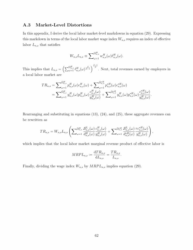
A.3 Market-Level Distortions

In this appendix, I derive the local labor market-level markdowns in equation (29). Expressing

this markdown in terms of the local labor market wage index Wn,s requires an index of effective

labor Ln,s that satisfies

Wn,sLn,s ≡∑ΩHn,s

ω=1wHn,s(ω)`Hn,s(ω).

This implies that Ln,s =(∑ΩHn,s

ω=1 `Hn,s(ω)

ββ−1

)β−1β

. Next, total revenues earned by employers in

a local labor market are

TRn,s =∑ΩHn,s

ω=1pHn,s(ω)cHn,s(ω) +

∑Ω∗Hn,s

ω=1p∗Hn,s(ω)c∗Hn,s(ω)

=∑ΩHn,s

ω=1yHn,s(ω)pHn,s(ω)

cHn,s(ω)

yHn,s(ω)+∑Ω∗Hn,s

ω=1yHn,s(ω)p∗Hn,s(ω)

c∗Hn,s(ω)

yHn,s(ω).

Rearranging and substituting in equations (13), (24), and (25), these aggregate revenues can

be rewritten as

TRn,s = Wn,sLn,s

(∑ΩHn,s

ω=1

SLn,s(ω)

dHn,s(ω)

cHn,s(ω)

yHn,s(ω)+∑Ω∗Hn,s

ω=1

SLn,s(ω)

d∗Hn,s(ω)

τc∗Hn,s(ω)

yHn,s(ω)

),

which implies that the local labor market marginal revenue product of effective labor is

MRPLn,s :=dTRn,s

dLn,s=TRn,s

Ln,s.

Finally, dividing the wage index Wn,s by MRPLn,s implies equation (29).

62

A.4 Proof of Proposition 2

To ease notation, suppose that every firm sells to both markets.86 Aggregate effective labor

is87

L =

∫ 1

0

NH∑n=1

Ln,sαα−1 ds

α−1α

.

Using the production function in equation (13) and output market clearing constraint in

equation (14), aggregate productivity Φ can be expressed as

Φ := C/L =

∫ 1

0

NH∑n=1

ΩHn,s∑ω=1

(cHn,s(ω)/C

φHn,s(ω)+τc∗Hn,s(ω)/C

φHn,s(ω)

) ββ−1

α(β−1)β(α−1)

ds

−α−1

α

. (35)

Let D and Dn,s denote the aggregate and local labor market total distortions in Home,

respectively. Defining the aggregate distortion as D := W/PΦ

and the market-level distortion

as Dn,s := Wn,s/PsΦn,s

, under Assumption 1 aggregate productivity can be rewritten as

Φ =

∫ 1

0

NH∑n=1

((SLn,s

)− θα

(Dn,s

D

)θΦn,s

θ−1

) αα−1

ds

α−1α

1θ−1

, (36)

where local labor market productivity Φn,s is

Φn,s =

ΩHn,s∑ω=1

(SLn,s(ω)−

γβφHn,s(ω)γ−1

[(dHn,s(ω)

Dn,s

)γ

+ τ 1−γ

(d∗Hn,s(ω)

Dn,s

)γ]) ββ−1

β−1β

1γ−1

. (37)

In an environment where distortions are constant across firms and markets, dHn,s(ω) =

d∗Hn,s(ω) = Dn,s = D. In this case, aggregate productivity is

Φd =

∫ 1

0

NH∑n=1

((SL,dn,s

)− θα(

Φdn,s

)θ−1) α

α−1

ds

α−1α

1θ−1

, (38)

86This implies that ΩHn,s = ΩHn,s = Ω∗Hn,s and Ω∗F

n,s = Ω∗Fn,s = ΩFn,s. Under Assumptions 1 and 2, this proof is

easily extended to a setting where some firms sell to only one market as long as the sets of firms selling toeach market is exogenous.

87This result also holds when aggregate productivity is defined in terms of total labor LH rather than totaleffective labor L, since L = λΓL

H .

63

where

Φdn,s =

ΩHn,s∑ω=1

(SL,dn,s (ω)−

γβφHn,s(ω)γ−1

[1 + τ 1−γ]) β

β−1

β−1β

1γ−1

, (39)

and SL,dn,s and SL,dn,s (ω) are the local labor market and firm-level shares of labor when distortions

are constant, respectively. These are also the first best levels of aggregate and local labor

market productivities that a planner would choose if it were subject to the iceberg trade

costs and upward sloping labor supply curves. Heterogeneity in distortions causes some firms

to be too large and other firms to be too small relative to the planner’s allocation. When

α < β, more productive firms are too small relative to their less productive local competitors.

If instead α > β, more productive firms are too large relative to their less productive local

competitors. Moving to an environment with constant distortions alleviates this source of

allocative inefficiency. However, as can be seen in the experiments in Section 5.1, with a fixed

number of firms and with variable markups, aggregate productivity need not be smaller with

variable markdowns than with constant markdowns when α > β.

Because workers have idiosyncratic match-specific productivities, such a move to a constant

distortion environment implies a novel tradeoff reflected in the SLn,s(ω)−γβ and

(SLn,s

)− θα terms

in the above equations. Focusing on the former, the inclusion of this term in the local labor

market productivity implies that a negative effect of increasing the size of an employer is

the reduced average match-specific productivity of workers. Intuitively, shifting workers to a

given employer can have a negative effect on aggregate productivity because some of those

workers would be more productive at a different employer.

That the exponent of this term depends on γ and β highlights how aggregate productivity

depends on a balance between love-of-variety in preferences and workers’ match-specific

productivities. As γ increases, varieties from the same sector become closer substitutes

for one another and the local labor market productivity index increases if more labor is

allocated to the most productive firm in the market. As β increases, workers’ match-specific

productivities become more similar on average across employers in a given local labor market,

so local labor market productivity increases by shifting workers towards the most productive

firms in the market.

B Data Appendix

This appendix describes the sample selection criteria for the ASI data and the crosswalks

used to map import data into Indian four-digit sectors.

64

The ASI samples are from all plants that are listed as registered manufacturers. In the

estimation sample, I include all plants that report the variables necessary to construct labor

costs, value added, sales shares, and employment and that report zero export revenues. Labor

costs are measured as total wages paid to all employees and any non-wage benefits reported.

I include wages for all employees because the non-wage benefits cannot be apportioned to

different categories of workers (i.e., production workers and managers) in a consistent way

across plants. Value added is measured according to guidelines in the ASI documentation.

Sales shares are constructed using data on revenues of all firms selling in a four-digit sector

and the share of Indian firms in total sectoral sales once imports are calculated. Employment

is measured in terms of mandays worked as this is the primary unit used in the ASI for

recording the quantity of labor used. As the ASI is designed as a representative survey rather

than a census, I use sample weights to compute the total sales of Indian firms in a sector

and total employment in a district-sector labor market. I exclude firms from the sample

that report negative labor costs or sales or have gross value added that is smaller than their

labor costs. Finally, I restrict the sample to plants in manufacturing sectors, i.e., they have

four-digit NIC-2008 codes between 1010 and 3300, inclusive. Of the 111,433 observations

across the two cross-sectional surveys, 55, 770 have usable data for each variable listed above,

meet these restrictions, and have a current status that is not recorded as being deleted from

the ASI sampling frame or non-existent. Of those plants, 50, 460 are non-exporters included

in the baseline regression specification.

To measure the total size of Indian sectoral product markets, I use import data from UN

Comtrade at the six-digit product level and a series of crosswalks to measure the import

share within each sector. The import data are available at the six-digit HS 2002 classification

level for the year 2008 and at the six-digit HS 2007 classification level for the year 2009.

I first map the 2008 data into the HS 2007 classification level using a crosswalk provided

by the UN Statistics Division.88 The HS 2007 product-level data can be mapped into the

Central Product Classification 2.0 (CPC2) using another UN provided crosswalk.89 In this

mapping, some HS 2007 codes map into multiple CPC2 codes. To avoid double counting,

I assume that the imports using HS 2007 codes are equally split across the corresponding

CPC2 codes. With imports measured at the CPC2 level, I use a final crosswalk provided by

the UN to map CPC2 codes into International Standard Industrial Classification Revision 4

(ISIC 4) industry-level codes.90 As with the previous mapping, some CPC2 codes map into

multiple ISIC 4 codes. I allocate these imports to the ISIC 4 codes by splitting them evenly

88This crosswalk is available at https://unstats.un.org/unsd/trade/classifications/correspondence-tables.asp89This crosswalk can be found at https://unstats.un.org/unsd/classifications/Family/Detail/107390This crosswalk is available at https://unstats.un.org/unsd/classifications/Family/Detail/27

65

across the relevant industry-level codes. With import data at the ISIC 4 industry level, the

total size of Indian four-digit NIC-2008 sectors can be calculated since, as noted in the ASI

documentation, these NIC-2008 codes are identical to the ISIC 4 codes.

C Model Extensions

C.1 Employer Choice with Non-Pecuniary Benefits

This appendix describes a variant of the model of employer choice developed in Section 2.1

where workers have non-pecuniary taste shocks for working at different employers rather

than match-specific productivity shocks. This model extends the framework developed in

Thisse and Toulemonde (2015) and Card et al. (2018). Workers are still endowed with a unit

of labor that they supply inelastically to their employer. However, the productivity of that

labor is the same for every worker at every employer. Employers are differentiated from each

other from the perspective of workers by an additional utility term that does not depend

on the wage offer of the employer. Suppose that indirect utility of a Home worker h that

chooses employer ω in location-sector pair (n, s) is

vn,s(h, ω) =wHn,s(ω) + Π

P+ εn,s(h, ω),

where the first term is the real income available to the worker for purchasing consumption

goods and the second term is an additive non-pecuniary taste shock.91 For brevity, denote by

vn,s(ω) =(wHn,s(ω) + Π

)/P the component of indirect utility that is common to all workers

at employer ω. Suppose the taste shocks are drawn independently across workers from the

following nested type I extreme value distribution

G(ε(h)) = exp

(−∑NH

n=1

(∫ 1

0

(∑ΩHn,s

ω=1exp

(−εn,s(h, ω)

β

))β/αds

)α).

Given the above specification of workers’ idiosyncratic preferences, the probability that

any given worker h chooses to work for employer ω is given by

SLn,s(ω) =exp (vn,s(ω)/β)

exp(Vn,s/β

) exp(Vn,s/α

)exp

(Vn/α

) exp(Vn)

exp(V) ,

91This formulation follows Thisse and Toulemonde (2015). If the taste shock is instead multiplicative, themodel is as in Card et al. (2018). In this alternative, the value of the taste shock to the worker depends ontheir wage level and aggregate profits and price levels.

66

where

Vn,s = β ln

(∑ΩHn,s

ω=1exp (vn,s(ω)/β)

)Vn = α ln

(∫ 1

0

exp(Vn,s/α

)ds

)V = ln

(∑NH

n=1exp

(Vn))

.

One key difference between the model in the main text and this alternative framework

is that with the same number of parameters, this alternative model implies that there are

asymmetric patterns of worker substitution across (n, s)-pairs because these local labor

markets are nested within sectoral labor markets. One cost of the Frechet distribution

assumption in the main text is that it requires an additional parameter to maintain the same

nested structure.92

While the version of the model with non-pecuniary motives for choosing different employers

offers more flexibility in terms of the patterns of worker substitution for the same number

of parameters, the cost of such a model is that labor supply elasticities depend on general

equilibrium variables. In this model, labor supply is just the product of the probability that

a worker chooses employer ω and the national labor endowment, i.e., `Hn,s(ω) = SLn,s(ω)LH .

The resulting labor supply elasticity is given by

ηLn,s(ω) =wHn,s(ω)

P

[1

β

(1− SLn,s(ω)

)+

1

αSLn,s(ω)

],

where SLn,s(ω) =(exp (vn,s(ω)/β) / exp

(Vn,s/β

))is the share of workers that choose location-

sector pair (n, s) that work for employer ω.

Labor supply elasticities now have two components that reflect the fact that workers

care about both the wage and the non-pecuniary benefit at their employer. The first factor

represents workers substitution patterns with regards to firms’ wage offers while the second

represents substitution patterns with regards to the non-pecuniary benefit. When firms

offer higher wages, then, all else being equal, they face more elastic labor supply. However,

since an increase in an employers’ wage, holding fixed all other firms’ wages, implies that

their labor market share also increases, the relationship between wages and labor supply

elasticities need not be monotonic. When α > β in this model, workers view jobs from the

same location-sector pair as being closer substitutes than those from different local labor

92The Frechet version with three nests is presented in Appendix C.3.

67

markets.93 In this case, labor supply elasticities are not strictly decreasing in the employers’

wage.

Estimating the labor supply elasticity parameters in this alternative framework is more

complicated because the elasticities depend on the aggregate price index. Therefore, the

elasticity parameters would need to be estimated in the full equilibrium of the model using a

simulated method of moments estimation strategy.

A similar problem arises if the specification of indirect utility follows the model in Card

et al. (2018). In this case, indirect utility can be written as vn,s(h, ω) = vn,s(ω)εn,s(h, ω).

Assuming that the log of the taste shocks are drawn from the same nested type I extreme

value distribution as above, the market share of total employment at employer ω is

SLn,s(ω) =vn,s(ω)(1/β)

¯Vn,s(1/β)

¯Vn,s(1/α)

¯Vn(1/α)

¯Vn¯V,

where

¯Vn,s =

(∑ΩHn,s

ω=1vn,s(ω)(1/β)

)β¯Vn =

(∫ 1

0

¯Vn,s1/α

ds

)α¯V =

(∑NH

n=1

¯Vn

).

The corresponding labor supply elasticity is

ηLn,s(ω) =wHn,s(ω)

wHn,s(ω) + Π

[1

β

(1− SLn,s(ω)

)+

1

αSLn,s(ω)

],

where SLn,s(ω) =(vn,s(ω)/ ¯Vn,s

)1/β

. In this case, the labor supply elasticity depends on the

aggregate per-capita dividend payment. Therefore, the estimation strategy used in the main

text to recover the structural parameters cannot be used, as the labor supply elasticity

depends on a general equilibrium variable.

93That is, the structural parameters here are the inverse of the corresponding parameters in the main text.

68

C.2 Labor Supply with Fixed Effects

Suppose that workers’ match-specific productivities are drawn from

G(ε(h)) = exp

(−λ∑NH

n=1λn

∫ 1

0

λn,s(∑ΩHn,s

ω=1λn,s(ω)εn,s(h, ω)−β)

α/β

ds

),

where λ, λn, λn,s, and λn,s(ω) are fixed productivity shifters that adjust the scale of the

distribution. This alternative productivity distribution implies (after repeating the steps in

Appendix A.1) that the probability that a worker h chooses employer ω is

λn,s(ω)wHn,s(ω)β

Wn,sβ

λn,sWn,sα

Wnα

λnWnα

Wα,

where

Wn,s =

(∑ΩHn,s

ω=1λn,s(ω)wHn,s(ω)β

)1/β

Wn =

(∫ 1

0

λn,sWn,sαds

)1/α

W =

(∑NH

n=1λnWn

α

)1/α

.

The average productivity of ω’s workers is now

λ1/α W

wHn,s(ω)Γ(1− 1/α).

Labor supply can be written as

`Hn,s(ω) = wHn,s(ω)β−1

Wn,sα−βΛn,s(ω),

where Λn,s(ω) = λn,s(ω)λn,sλnλ1/αW 1−αλΓL

H is an endogenous labor supply shifter that is

perceived as a constant by employer ω. The formula for a firm’s labor supply elasticity given in

equation (18) remains unchanged. Adding these fixed effects introduces additional exogenous

sources of workers’ comparative advantage. Furthermore, if these fixed effects are specific to

workers in each country, they enable an investigation of how differences across countries in

workers’ patterns of comparative advantage affect trade patterns and other outcomes. This

type of comparative advantage has been studied in Galle et al. (2018) and Lee (2020) (these

papers also allow for the shape parameters of the distribution of worker productivities to

69

be country-specific). Finally, the particular fixed effects presented in this appendix are an

example of how to incorporate additional flexibility into the model. Alternative models with

different nesting patterns are also possible.

C.3 Labor Supply with Additional Nests

This appendix describes two extensions to the labor supply model in the main text that allow

for an additional nest in order to break the symmetric pattern of worker substitution across

location-sector pairs. The first alternative assumes that workers’ match-specific productivities

are nested as follows: employers within an (n, s)-pair, (n, s)-pairs within sector s, and sectors

within location n. Suppose that the distribution of match-specific productivities is

G(ε(h)) = exp

−∑NH

n=1

(∫ 1

0

(∑ΩHn,s

ω=1εn,s(h, ω)−β)

α/β

ds

)ξ/α ,

where the new parameter, ξ, governs the dispersion of productivity draws across sectors

within locations. If ξ = α, this distribution collapses to the one in the main text. If ξ < α,

this distribution implies that workers find jobs within the same location, regardless of their

sector, as closer substitutes for one another on average as compared to jobs from different

locations.

Following the steps in Appendix A.1, this distributional assumption implies that the

probability that worker h chooses employer ω is(wHn,s(ω)

Wn,s

)β (Wn,s

Wn

)α(Wn

W

)ξ,

where wage indices are given by

Wn,s =

(∑ΩHn,s

ω=1wHn,s(ω)β

)1/β

Wn =

(∫ 1

0

Wn,sαds

)1/α

W =

(∑NH

n=1Wn

ξ

)1/ξ

.

The expected productivity of ω’s workers is now WwHn,s(ω)

Γ(1− 1/ξ), which implies that labor

70

supply can be written as

`Hn,s(ω) = wHn,s(ω)β−1

Wn,sα−βΛn,

where Λn = Wnξ−αW 1−ξΓ(1− 1/ξ)LH . While the labor supply curve is modified relative to

the one used in the main text, the assumption that there is a continuum of sectors implies

that the wage elasticity of labor supply remains unchanged and is given by equation (18).

The reason for this is that firms, in choosing their wages, correctly take the location-level

wage index Wn as a constant and only internalize the effect of their wage on the (n, s)-pair

wage index Wn,s. Introducing the additional nest in this way has no effect on the relationship

between market shares and market power, but requires estimation of an additional parameter

to compare outcomes under oligopsony and perfect competition in labor markets.

Suppose instead that workers’ match-specific productivities are drawn from

G(ε(h)) = exp

−∫ 1

0

(∑NH

n=1(∑ΩHn,s

ω=1εn,s(h, ω)−β)

α/β)ξ/α

ds

,

where ξ now governs the dispersion of productivity draws across locations within a sector.

When ξ < α, workers view jobs from the same sector as closer substitutes, on average, to

each other than jobs from different sectors, regardless of where those jobs are located.

Choice probabilities are now given by(wHn,s(ω)

Wn,s

)β (Wn,s

Ws

)α(Ws

W

)ξ,

where Wn,s is unchanged, and

Ws =

(∑NH

n=1Wn,s

α

)1/α

W =

(∫ 1

0

Wsξds

)1/ξ

.

Average productivity of ω’s workers is WwHn,s(ω)

Γ(1− 1/ξ), and the labor supply curve is

`Hn,s(ω) = wHn,s(ω)β−1

Wn,sα−βWs

ξ−αΛ,

where Λ = W ξ−1Γ(1− 1/ξ)LH . In contrast with the previous alternative nesting structure,

this version does change the relationship between firms’ size and their market power in labor

71

markets. Because there is a finite number of locations and a finite number of firms in each

sector, firms correctly internalize the effects of their wage choices on the sector-level wage

indices Ws. The resulting wage elasticity of labor supply perceived by the firm is

(β − 1) + (α− β)SLn,s(ω) + (ξ − α)SLn,s(ω)SLn,s,

where SLn,s = (Wn,s/Ws)α is the share of workers in sector s that work in location-sector pair

(n, s). The rate at which the labor supply elasticity decreases with a firm’s market share is

larger with this alternative nesting structure when ξ < α, because firms internalize the effects

of their size relative to the entire sector and not just relative to their location-sector pair.

Furthermore, firms in larger (n, s)-pairs (within their sector) face more inelastic labor supply.

C.4 Cournot Competition: Differentiated Jobs

In this appendix, I derive price elasticities of product demand and wage elasticities of labor

supply under the assumption that firms compete as Cournot oligopolists and oligopsonists.

Furthermore, the assumption that workers have idiosyncratic match-specific productivities

for working at different firms is maintained so that jobs are imperfect substitutes for one

another. In this alternative model, firms assume that their competitors’ quantity of output

produced and effective labor hired is fixed and that they adjust by changing their prices and

wages. As with the Bertrand model in the main text, a firm simultaneously chooses its total

output produced and quantity of effective labor hired.

For deriving elasticities under Cournot competition, it is convenient to rewrite the product

demand (equations (9) and (10)) and labor supply (equation (6)) curves as inverse demand

and supply curves. The Home inverse product demand function facing a Home producer is

pHn,s(ω) = cHn,s(ω)−1/γCs1/γ−1/θ∆1/θ,

while the inverse labor supply curve facing a Home producer is

wHn,s(ω) = `n,s(ω)1

β−1Ln,s1

α−1− 1β−1 Λ

−1α−1 ,

where Ln,s is an index of the total effective employment in location-sector pair (n, s). This

effective employment index is

Ln,s =

(∑ΩHn,s

ω=1`n,s(ω)

ββ−1

)β−1β

.

72

The functional form for this effective employment index emphasizes the structural similarities

between the CES preference model and the Frechet-Roy labor supply model. This can also

be seen by comparing the market shares. The Home sectoral product market revenue share

of a Home producer is

SHn,s(ω) =

(pHn,s(ω)

Ps

)1−γ

=

(cHn,s(ω)

Cs

) γ−1γ

.

The employment market share (both in terms of the share of (n, s)-pair workers that choose

employer ω and the employer’s share of local effective labor) is

SLn,s(ω) =

(wHn,s(ω)

Wn,s

)β

=

(`n,s(ω)

Ln,s

) ββ−1

.

From the inverse product demand curve, the Home price elasticity of demand under the

Cournot assumption is

ηHn,s(ω) =

(1

θSHn,s(ω) +

1

γ

(1− SHn,s(ω)

))−1

.

The wage elasticity of labor supply when firms compete as Cournot oligopsonists is given by

ηLn,s(ω) =

(1

α− 1SLn,s(ω) +

1

β − 1

(1− SLn,s(ω)

))−1

.

As with the wage elasticity of labor supply under Bertrand competition, the Cournot elasticity

takes on a functional form that is analogous to the price elasticity of demand. The relationship

between firms’ market shares and market power depends on the relative magnitude of α and

β. If, as in the main text, α < β, then larger employers face more inelastic labor supply and

hence have more market power in their local labor markets.

C.5 Endogenous Market Entry

As discussed in Section 2.7, the production and pricing decisions of a firm that sells in both

the Home and Foreign markets are interdependent because firms have increasing marginal

costs. This feature of the model complicates market entry decisions both for a given firm and

in general equilibrium and implies that equilibrium selection rules used in the literature to

endogenize market entry cannot be used without amendment when firms have market power

73

in labor markets.94

Entry decisions in heterogeneous firm trade models typically rely on fixed costs specified

in terms of either labor or some good, neither of which firms can affect the price of directly,

as the arbiter of which firms are active in each market. In this model, there are two distinct

types of assumptions. First, firms could be required to spend a fixed amount of the final

good (either their domestic one or market-specific ones) to enter a market. In this case firms’

costs of production would not depend on these fixed costs of production.95 In contrast, in

the second case firms could be required to hire a fixed amount of labor or use a fixed amount

of their own output to enter a market, which would cause the extensive margin of entry to

affect firms’ costs through these fixed requirements. Suppose that the latter case holds and

Home (Foreign) firms must hire a fixed amount of labor fd (f ∗d ) and f ∗x (fx) to enter into the

domestic and export markets, respectively.

Denote by πHn,s(ω,m) the total profits of Home firm ω that solve equation (15) when it

sells to markets m ∈ ∅, H, F,HF, where m = ∅ implies the firm sells to neither Home nor

Foreign and m = HF implies they sell to both markets. The following definition gives a

notion of a stable equilibrium with endogenous market entry decisions for given aggregate

variables.

Definition 2. An equilibrium is stable if for each firm ω the firm, taking as given its set of

sector s product market competitiors and (n, s)-pair labor market competitiors and aggregate

shifters ∆,∆∗,Λ,Λ∗, sells to the set of markets m such that πjn,s(ω,m) ≥ πjn,s(ω,m′) for

any m′ 6= m and j ∈ H,F.

Stability of entry decisions is a unilateral concept. Each firm chooses the markets that

maximize profits and internalizes the effects of their entry decisions on sectoral price indices Ps

and P ∗s and local wage indices Wn,s or W ∗n,s. As is common in many oligopoly environments,

there can be many potential stable equilibria for a given set of potentially active firms.

For this reason, equilibrium selection rules are used to isolate equilibria that are uniquely

94In the main text, I assume away the problem of determining the sets of firms that sell to each market byassuming they are given exogenously. I make this assumption because of the considerable increase in thecomplexity of endogenizing these decisions relative to other work using oligopoly models of trade, includingAtkeson and Burstein (2008), Eaton et al. (2013), Edmond et al. (2015), and Gaubert and Itskhoki (2018). Inan environment where these margins are endogenous, the problem of determining the optimal set of marketsto sell to shares many similarities with Antras et al. (2017). Whereas in that setting the decision to sourceinputs from a given market is a complement to the decision to source inputs from other markets, here thedecision to sell output to a given market is a substitute for the decision to sell output to the other market.Arkolakis and Eckert (2017) offer a generalized analysis of models in which extensive margins are eithercomplements or susbtitutes and show how solving these problems in general equilibrium is a challengingcombinatorial problem. They offer an algorithm that finds a solution to the problem in general equilibrium,but the algorithm does not give a unique equilibrium.

95In a richer model, an input over which firms have no market power could be used, such as perhaps capital.

74

determined by certain properties deemed to be desirable.96

In an environment with perfectly competitive labor markets, the entry decisions can be

solved for each national product market independently. The typical selection rule, following

Atkeson and Burstein (2008), is to order firms in a sector by their total factor productivities

and consider a sequential entry game that leads to a stable equilibrium in which each firm in

the sector from a given country that sells to a national product market is more productive

than any firm from that same country and sector that does not sell to that market.97

If firms have market power in labor markets, entrants into both markets must be determined

simultaneously. When fd = 0 for all Home firms and f ∗d = 0 for Foreign firms, as is the case in

Atkeson and Burstein (2008), every firm sells in its domestic market and the set of exporters

is endogenous. However, refinements to their equilibrium selection rule are required since

one needs to determine which country’s best firm makes its export entry decision first. For

example, suppose that in a given sector there is a single firm in each country and consider

the problem facing the Home firm. Because marginal costs are increasing, the profitability of

exporting for the Home firm depends on how much it sells domestically.98 But the amount

that the Home firm sells domestically depends on whether or not the Foreign firm sells to

the Home market, so the Home firm can be crowded out of exporting when the Foreign firm

exports. Therefore, one needs to choose which country’s firm makes its export entry decision

first. When there are multiple firms in a sector in each country, this choice cannot solely

depend on firms’ total factor productivity rankings, since differences in the profitability of

exporting for two firms from different countries depends on both their exogenous local labor

market conditions and differences across countries in the product market environment.99

When fd > 0, as in Eaton et al. (2013), Edmond et al. (2015), and Gaubert and Itskhoki

(2018), entry decisions are even more complicated. Suppose that there is a single production

location in each country so that within a sector each country’s firms can be ranked by their

productivities. With labor market power, entry into operation (i.e., selling to either market)

by a firm increases competition in the labor market, which raises wages for all other firms in

96For example, the property that entry by any given firm into a market is not crowded out by a less efficientfirm from the same country selling there.

97This sequential entry game is also used in Eaton et al. (2013), Edmond et al. (2015), and Gaubert andItskhoki (2018).

98To emphasize, profitability does not refer to the profits earned from the export market. Instead,profitability refers to the incremental total profits from entering the export market, πHn,s(ω,HF )− πHn,s(ω,H).Profits earned from the export market must be positive for incremental profits to be positive, but this is nota sufficient condition since entering into exporting reduces profits from the domestic market.

99Another wrinkle with labor market power is that in a stable equilibrium it is possible that an exporter hasa higher marginal cost than a firm from the same country that does not export even though the exporter hasa higher total factor productivity than the non-exporter and even if the two firms being compared produce inthe same (n, s)-pair.

75

that sector and country. Prices of these firms increase in any market to which the firms sell.

For firms in the entrant’s country that were exporting, this entry into operation can make

exporting unprofitable.100 Therefore, in the context of a sequential entry game one needs to

check whether the entry decisions in both markets of firms that act earlier in the game are

robust to entry of firms later in the game.

Reintroducing multiple production locations within a country adds another layer of

complication to determining a stable set of entrants since entrants affect firms from their own

(n, s)-pair by more than they affect other competitors within their sector. As mentioned in

Section 2.4, exogenous heterogeneity in the set of local labor market competitors means firms

within a country cannot be ranked only by their productivities. Furthermore, entry by a second

firm that produces in an (n, s)-pair in which there is already a first firm operating can change

the ranking of the first firm relative to all other firms from the entrant’s country because the

competition for labor from the second firm affects its local labor market competitors more

closely than other firms. This makes the problem of having to check the entry decisions of

previous entrants in a sequential entry game described in the last paragraph more complicated

since the ranking of the previous entrants can change.

Given the intricacies in modelling market entry decisions when firms have labor market

power, solving for a stable equilibrium is computationally demanding, so I leave this problem

for future research.

100If the entrant sells domestically, entry can make exporting unprofitable for firms from the other country,particularly if there are differences in fixed labor requirements for selling to the entrant’s country. This is alsotrue in the sequential entry game in Edmond et al. (2015) since there fixed costs of selling domestically arenot necessarily the same as fixed costs of exporting. In Eaton et al. (2013) and Gaubert and Itskhoki (2018),firms from either country pay the same fixed cost to sell to a given market, so this problem does not arise.

76