Trade Adjustment Assistance and Pre-Displacement Wages

Frank Barry Trinity College Dublin

Eric Strobl

Ecole Polytechnique

Frank Walsh1 University College Dublin

July 2007 Abstract This paper investigates how Trade Adjustment Assistance (TAA) affects pre-displacement wages in imperfectly competitive labour markets, using both an efficiency wage and a bargaining model. Our results reveal that under both frameworks employment subsidies for displaced workers raise pre-displacement wages. By contrast, subsidies to unemployed displaced workers unequivocally raise pre-displacement wages only in the bargaining model.

1 Corresponding author. School of Economics, Room G214 Newman building, University College Dublin, Belfield Dublin 4, Ireland. Email:Frank.walsh@ucd.ie, Phone: 35317168697, Fax: 35312830068.

2

Trade Adjustment Assistance and Pre-Displacement Wages

July 2007

Abstract This paper investigates how Trade Adjustment Assistance (TAA) affects pre-displacement wages in imperfectly competitive labour markets, using both an efficiency wage and a bargaining model. Our results reveal that under both frameworks employment subsidies for displaced workers raise pre-displacement wages. By contrast, subsidies to unemployed displaced workers unequivocally raise pre-displacement wages only in the bargaining model. Section I: Introduction

While trade liberalisation can be hugely beneficial on aggregate, there will almost

invariably be groups who lose out over the course of the adjustment process. In this

regard it is widely recognised that compensating dislocated workers, besides smoothing

the cost of frictional unemployment, can help defuse opposition to liberalisation by

distributing some of the gains to these groups. As a matter of fact, survey evidence

provided by Sheve and Slaughter (2001) indicates that a majority of American workers

would be in favour of further liberalization provided that those who are harmed receive

some sort of compensation or assistance.

Trade adjustment assistance represents one such form of compensation. Baicker

and Rehavi (2004) provide a review of the history of trade adjustment assistance (TAA)

in the US. It was formally introduced in the US Trade Expansion Act of 1962 to

3

compensate workers for tariff cuts under the Kennedy Round of multilateral negotiations.

Similar provisions were included in the Canadian-American Auto Agreement, the

Manpower Development and Training Act of 1962 and the Economic Opportunity Act of

1964. A separate trade adjustment assistance programme was introduced for job

disruptions associated with NAFTA in the early 1990s. In 2002 the US Congress

demanded a substantial expans ion of TAA in exchange for the renewal of Presidential

trade negotiating authority. The 2002 Act expanded eligibility to secondary workers at

an affected firm’s upstream suppliers and downstream customers and to workers laid off

in plant relocations. In addition, cash benefits to workers in certified firms were extended

to 78 weeks rather than the previous 52, and higher job search and relocation allowances

were made available. A new pilot scheme, as proposed by Kletzer and Litan (2001), was

also introduced for workers aged 50 and above. This provides them with cash benefits

equal to 50 percent of the difference between their new and old salaries if reemployed at

lower wages within 26 weeks of separation, subject to earnings of less than a set amount,

and also offers temporary subsidies to help pay for health insurance.

Interest in TAA has expanded further in recent times. One of the first bills

introduced in the new Democratically-controlled US Senate would expand TAA to cover

not only manufacturing workers but also service workers whose jobs are deemed to have

been offshored, and would offer help not just to individual factories but to entire

industries. Germany since 2003 has operated a scheme which sees the government make

up 50 percent of the wages lost by people above a certain age who are forced into a lower

paying job, while France operates a similar scheme without age restrictions. More

4

recently, the European Union has created a €500 million ($650 million) fund to help

those who lose their jobs because of “structural changes in world trade patterns”.

Possible adverse effects of such types of schemes have been identified by Baicker

and Rehavi (2004). Noting the well-documented spike in the likelihood of an

unemployed worker being reemployed at the time that benefits expire, they point out that

increasing the generosity and length of time for which TAA benefits are available could

increase the average duration of unemployment, while the wage subsidies offered to

bridge the gap between workers’ new and old salaries reduce the incentive to seek out the

highest-paying ava ilable jobs. They also point out that firms may be induced to lay off

workers seasonally because they pay less in unemployment insurance taxes than workers

receive in benefits for each layoff.

From a theoretical perspective, Brecher and Choudhri (1994) or iginally

demonstrated that the Dixit and Norman (1986) result that commodity taxes could be

used to compensate the losers without exhausting the benefits from freer trade may not be

possible in the presence of unemployment. Feenstra and Lewis (1994) show that similar

problems also arise when factors of production are imperfectly mobile, though they

suggest that the use of commodity taxes coupled with trade adjustment assistance may be

adequate to achieve true Pareto gains from liberalization. As Davidson and Matusz

(2005) point out, however, Feenstra and Lewis do not address the question of whether

there may be a superior way to achieve this goal. Davidson and Matusz (2005) thus set

themselves the goal of finding the labor market policy that fully compensates declining-

sector workers while imposing the smallest distortion on the economy. They find that the

5

best package consists of a wage subsidy to those who switch sectors after liberalization,

combined with an employment subsidy to the declining sector. 2

The literature on trade adjustment assistance, however, typically ignores the

possible impact of such a policy on pre-displacement wages. In Davidson and Matusz

(2005), for example, the wage paid reflects the marginal productivity of labour which

remains unchanged in the face of TAA. In imperfectly competitive labour markets, by

contrast, the wage is also typically influenced by the workers’ outside option, and this in

turn is influenced by the presence or absence of a trade adjustment assistance program3.

This insight accords well with the logic of TAA as discussed above. If workers are more

likely to support trade liberalisation in the knowledge that they will be compensated in

the event of job loss, it implies that fear of displacement, and hence the perceived outside

option, is affected by the policy. Thus, TAA may feasibly drive up the wages of workers

in potentially eligible firms, raising the possibility that trade adjustment assistance further

increases the likelihood of displacement. Under what circumstances this may happen is

therefore clearly important for properly evaluating the possible effects of TAA on the

labour market.

In this paper we set out to explicitly model the impact of TAA on pre-

displacement wages within an imperfectly competitive labour-market framework. In this

regard we resort to commonly used models of imperfectly competitive labour markets:

2 Barry (1995) critiques an earlier literature on optimal intervention in the presence of arbitrary wage rigidities that concluded that some degree of subsidisation of the declining industry is warranted on efficiency grounds. His bargaining model generates wage stickiness and inefficiently low levels of inter-sectoral labour transfer. Optimal intervention in this case entails supporting expanding rather than declining sectors. 3 There are of course special cases, such as when workers are identical, where the equilibrium wage will equal the outside option for workers in a competitive labour market. In this instance TAA to unemployed displaced workers will price affected workers out of the market and certainly cause displacement. In imperfectly competitive labour markets the dependence of the equilibrium wage on the outside option is more fundamental and will be true in more general settings such as with worker heterogeneity.

6

the efficiency-wage shirking model and the bargaining model. Our results show that

under both efficiency wage and bargaining model frameworks employment subsidies for

displaced workers raise pre-displacement wages. In contrast, while a similar effect is

found for subsidies to unemployed displaced workers in the bargaining model, whether

such TAA will raise the pre-displacement wage of the unemployed under the efficiency

wage framework will depend on the particular parameter values prevailing.

The remainder of the paper is organized as follows. In the following section we

outline the basic structure of our framework. Section III then introduces wage setting

under the shirking model and isolates the effect of employment and unemployment

subsidies on pre-displacement wages. In Section IV we alternatively assume that firms

bargain over wages within a matching/union model and similarly investigate how

subsidies impact on pre-displacement. Concluding remarks are provided in the final

section.

Section II: The General Framework

There are two periods, one and two. Workers who are displaced in the first period

and acquire a job in the second receive a wage or employment subsidy. The intention is

to model the temporary subsidisation of employment or unemployment of workers who

are displaced as a consequence of trade liberalisation. We explore the issue in both a

bargaining model and a shirking efficiency-wage model.

The expected utility of the state the worker is in equals: iKLMV . The i superscript is

either n or s for non-shirking or shirking while the subscript K is either E for employed or

7

U for unemployed, an L subscript means the individual lost his or her job at the end of the

first period (is displaced) and the subscript M is either 1 or 2 for the first or second period

respectively. Workers discount second period utility by a factor ß. The timing of the

model is as follows:

(1) The wage for period one (yE1) is determined at the beginning of the period and

firms choose the level of effort (x1) which will imply a wage that is consistent

with the worker’s incentive not to shirk at that level of effort. Firms also

choose employment. Some workers may be unemployed since the wage is

above the competitive level if monitoring is imperfect. There may also be

frictional unemployment.

(2) Employees either work or shirk, and firms supervise.

(3) At the end of period one there is an exogenous probability b that workers will

be fired due to random negative shocks to firms. There is also a probability q

that a shirking worker will be caught. If caught, they are fired. All those in

employment receive the pre -displacement wage agreed upon at the beginning

of period one while unemployed or fired workers receive the unemployment

benefit (yU1).

(4) All workers, including those fired or otherwise unemployed, apply for period

two jobs.

(5) At the beginning of period two, firms choose the level of employment and

unemployed workers get jobs with probability e. The wage yE2, which will be

paid at the end of the period, is set. TAA payments to eligible employed and

unemployed workers are also made at the end of this period

8

(6) Employees either work or shirk, and employers supervise.

(7) At the end of the second period, non-shirkers and those not caught shirking

are paid the wage. Workers who are caught shirking are fired and do not

receive a wage. Those workers who lost their jobs in the previous period but

found a new job at the beginning of the second period receive the wage plus

an employment subsidy: (yEL2+sE). Unemployed workers who were also

unemployed in the first period receive the unemployment benefit (yU2), while

those unemployed workers who became unemployed at the end of period one

get higher benefits (yU2). Workers who were employed in period one,

continue to be employed at the beginning of period two and get fired for

shirking in period two get: sUy 2 . This equals unemployment benefits (yU2) plus

some fraction e of the unemployment subsidy sU. That is, given the discrete

nature of the model it may be unreasonable to assume that workers who lose

their job at the end of period one are displaced and qualify for full

unemployment subsidies, while another worker who had been employed in

period one but gets fired for shirking in period two (perhaps close to the

beginning of the second period) gets unemployment benefits but no subsidy. 5

Finally, workers who lose their job at the end of period one, succeed in

finding a new job (and thus qualify for employment subsidies) but get fired for

shirking receive sULy 2 . This equals 2Uy plus some fraction a of the

employment subsidy (sE). Because of the discrete nature of the model,

5 Workers displaced during the second period can be assumed to be displaced only at the end of the second period and thus receive the full second-period wage.

9

workers who are caught shirking get fired and do not receive any wage from

the firm. Of course, in reality we would expect that such workers would have

been working for part of the second period before being fired and to have

benefited somewhat from the subsidy. For this reason we allow for the

fraction of the employment subsidy that workers who are fired get to keep

(alpha) to be positive.

To help clarify the payments received by a worker in each state we include two graphs in

the Appendix. The first graph shows all the possible states and payoffs for a worker who

is unemployed at the beginning of period one, while the second shows the possible states

and payoffs for an initially employed worker.

Section III: Wage Setting under the Shirking Model

The best known shirking model of efficiency wages is arguably that of Shapiro

and Stiglitz (1984) . They look at a stationary equilibrium for inf initely lived agents. We

look at a discrete time analogue of the model to analyse the impact of temporary

subsidies.6

6 Given that there are only two periods we might worry that the game is not incentive compatible since agents would cheat in the terminal period. Kandori (1992) shows in an overlapping generations game that incentive compatibility conditions can be sustained in this type of game if the current generation has knowledge on how previous generations played the game. This suggests intuitively at least that we could formulate the game in this paper with finitely lived agents and still satisfy incentive compatibility if we repeat the two period game in an overlapping generations framework.

10

We assume workers have full information and know all the parameters of the

model, including the probability of shocks that might affect their employer. The first

period serves to identify the workers eligible for TAA.

The expected utility of a non-shirker who is employed in period one is:

22111 )1()( EULEn

E VbVbxgyV ββ −++−= (1)

This is the wage income less disutility of effort plus the expected utility of unemployment

in the second period if the worker is displaced times the probability of displacement, plus

the expected utility of employment in the second period times the probability of this

outcome. 7 The expected utilities of employment and unemployment in period two will be

defined below.

The expected utility of a shirker who is employed in the first period is:

22111 )]1)(1(1[)1)(1()1( ULEUEs

E VqbVqbqyyqV ββ −−−+−−++−= (2)

This is the wage times the probability of not being caught shirking, plus benefits times

the probability of being caught, plus the probability of not being displaced in the first

period (1-b)(1-q) times the expected utility of second period employment, plus the

probability of being displaced times the expected utility of second period unemployment

for a displaced worker.

The expected utility of an individual who is unemployed in the first period is:

211 UUU VyV β+= (3)

7 When a worker in the first period anticipates the value of employment in the second period they anticipate the no-shirking condition will be satisfied in the second period . This determines the value of the job as will be seen below.

11

This is just benefits plus the expected present value of second period unemployment

which is defined below. The expected utility of unemployment for a previously

unemployed worker in the second period is:

2 2 2(1 )U U EV y e eV= − + (4)

This is the discounted value of second period benefits times the probability the worker

will not find a job at the beginning of the second period, plus the probability the worker

will find a job times the discounted expected utility of a job for a non-displaced worker.

The expected utility of second period unemployment for a displaced worker is:

222 )1)(( ELUUUL eVesyV +−+= (5)

This is the same as (4), though for a displaced worker.

The expected utility of not shirking in the second period for a worker who was

unemployed in the first period but gets a job in the second is:

)( 222 xgsyV EELn

EL −+= (6)

This is just the value of the difference between earnings and the disutility of effort for a

displaced worker in the second period.

The expected utility of shirking in the second period for a worker who was

unemployed in the first period but gets a job in the second is:

)()1)(( 222 EUEELs

EL syqqsyV α++−+= (7)

This is the wage for a previously displaced worker who gets a job in the second period

times the probability of not being caught shirking times the value of benefits times the

probability they will be caught.

The expected utility of not shirking in the second period for a worker who was

employed in the first period and remains employed in the second is:

12

)( 222 xgyV En

E −= (8)

This is the same as (6), though for a non-displaced worker.

The expected utility of shirking in the second period for a worker who was

employed in the first period and remains employed in the second is:

)()1( 222 UUEs

E syqqyV ε++−= (9)

This is the same as (7) for a non-displaced worker except we assume that a worker who is

fired for shirking gets to keep a fraction e of the additional benefits that displaced workers

get. For the efficiency wage equilibrium we solve for the wage that satisfies the no-

shirking condition for a second period workers: sE

nE VV 22 = .

UUE syqxg

y ε++= 22

2

)( (10)

For displaced workers who get a job in the second period the no shirking condition and

wage are : sEL

nEL VV 22 =

EUEL syqxg

y )1()(

22

2 α−−+= (11)

A fraction (1-a) of employment subsidies will be passed onto employers in lower

wages while displaced workers’ wages increase by aSE. This implies that displaced

workers will be cheaper than others, raising the possibility that firms will fire other

workers in order to hire subsidised displaced workers. 8

From these equations we substitute the no-shirking conditions above into (6) and

(8) to get the equilibrium expected utility of a second period job for non-displaced and

displaced workers respectively, if the no-shirking condition holds with equality: 8 For example Breen and Halpin (1989) find that only 20 percent of jobs under the employment incentive scheme in Ireland were additional. This scheme gave subsidies to firms who hired unemployed workers.

13

])()1(

[ 222 UUE syxgq

qV ε++

−= (12)

])1()()1(

[ 222 EUEL syxgq

qV α−−+

−= (13)

We substitute (12) and (13) into (1) and (2), i.e. we assume that the equilibrium holds in

the second period, and substitute the equilibrium expected utility of a second period job

into the equation for the expected utility of a first period job. This allows us solve for the

no-shirking condition in the first period: sE

nE VV 11 = as

}])1[()(

)1)(1{()1()(

])[1()(

21

1

2211

1

EUU

ULEUE

esseqxg

qebyqxg

VVbyqxg

y

αεβ +−−+−−−−+

=−−−+= (14)

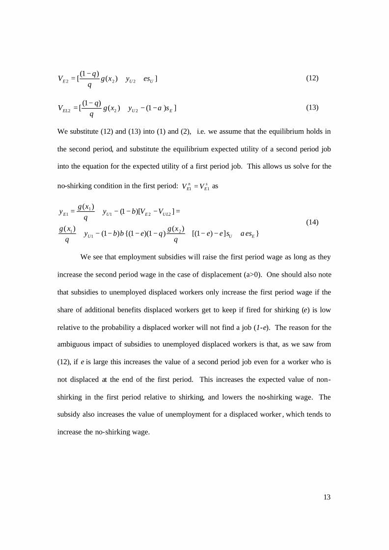
We see that employment subsidies will raise the first period wage as long as they

increase the second period wage in the case of displacement (a>0). One should also note

that subsidies to unemployed displaced workers only increase the first period wage if the

share of additional benefits displaced workers get to keep if fired for shirking (e) is low

relative to the probability a displaced worker will not find a job (1-e). The reason for the

ambiguous impact of subsidies to unemployed displaced workers is that, as we saw from

(12), if e is large this increases the value of a second period job even for a worker who is

not displaced at the end of the first period. This increases the expected value of non-

shirking in the first period relative to shirking, and lowers the no-shirking wage. The

subsidy also increases the value of unemployment for a displaced worker , which tends to

increase the no-shirking wage.

14

Section IV: Wage Setting Under a Bargaining Model

The two most common applications of the bargaining model in the labour

literature are to model unionised labour markets [see Booth (1995)] or to solve the wage

in a matching model where there is a match-specific surplus when a worker and employer

meet (Pissarides 2000). While the model analysed below is closer to the matching model

in that we model a bargain between an individual worker and firm, it can also be applied

to union wage models. For example Lindbeck and Snower (1991) assume workers

bargain only over the wage, and justify the assumption in terms of a pure insider-outsider

model where workers are unconcerned with the plight of outsiders. Oswald (1993)

develops a model that further rationalises this assumption. In his model there is a first-in

last-out rule for firing combined with a median voter who determines union elections.

Unless there are very large adverse shocks, the median voter’s job is secure and the union

bargains only over wages and working conditions, while the firm chooses employment on

the labour-demand curve. One should also note that whether the union cares about

employment possibly depends on the institutional framework (see Booth, 1995, for a

discussion) although in many cases it appears that unions accept the firm’s right to

manage when it comes to the choice of employment [see Oswald (1993) for anecdotal

evidence on this point].

In this section we assume there is perfect monitoring so that workers never shirk,

simplifying stages two and six in the timing of the model. The payoffs to workers are

now just the payoffs to non-shirkers in the previous section. The value of a job in the

second period is given by (6) and (8) for displaced and non-displaced workers

respectively and the value of a first period job by (1). We amend the expected utility of

15

unemployment in each time period [given by (3), (4) and (5)]. The reason for this is that

the motivation for the matching model analysed below is that there is some individual-

specific surplus that will be lost to both parties if they fail to strike a bargain. It is

therefore unreasonable to let the utility of an alternative job the worker may find with

probability e have the same utility as the job that is bargained over. For this reason we

get:

222 )1( EUU VeeyV +−= (4’)

222 )1)(( ELUULUL VeesyV +−+= (5’)

The )(( 22 2xgyV

EE −= and EEEL sVV += 22 terms are the exogenously given values of a

typical alternative second-period job for a non-displaced or displaced worker

respectively. We assume that worker’s productivities in the two periods are p1 and p2

respectively. The firm maximises expected profits in each period:

111 Eyp −=π (15)

222 Eyp −=π (16)

While the above equations give profits for firms that stay in business we define )1,0(∈S

as a firm-level technology shock that is equal to one or zero. In each period there is a

probability b that any firm will face a negative shock and be forced to shut down. The

firm makes zero profit if it shuts down. As a first step to solving the bargaining problem

we define the second period expected surplus from employment to workers who are

respectively eligible and not eligible for TAA:

222222 )1()( EUEUE VeeyxgyVV −−−−=− (17)

and:

16

222222 )1)(()1()( EUEUELULEL VeesseyxgyVV −−−+−−−=− (18)

We note that unemployment and employment subsidies have the opposite affect.

Employment subsidies increase the payoff to employment increasing the worker’s surplus

at any wage, while unemployment subsidies increase the value of the outside option and

lower the employment surplus at a given wage. Firm and worker’s bargaining power are

given by ? and (1-?) respectively. The objective function for the second period Nash

bargain for firm bargaining with displaced workers is the product of the firm’s and the

worker’s surplus weighted by their bargaining power:

)1(2222221 )]1)(()1()([)( θθ −−−+−−−−−=∆ essVeeyxgyyp UEEUELEL (19)

Taking first order conditions we can solve for the wage that solves the second period

bargaining problem for a displaced worker:

)]1)(()([)1( 22222 essyVexgpy EUUEEL −−++++−= θθ (20)

The post-displacement bargained wage is increasing in the unemployment subsidy

and decreasing in the employment subsidy. Of course since the employed worker

receives the employment subsidy this is equivalent to saying that (1-e) of the employment

subsidy is passed on to the firm in the form of lower wage costs while e of the

employment subsidy goes into higher take -home pay. If we do the same for a non-

displaced worker the wage is:

)]1()([)1( 22222 eyVexgpy UEE −+++−= θθ (21)

We recognise that if workers fail to strike a bargain in the first period the match is

dissolved and the second period surplus is lost to both players. In this event the firm gets

nothing and the worker receives VU1 [given in equation (3)]. For this reason, in the first

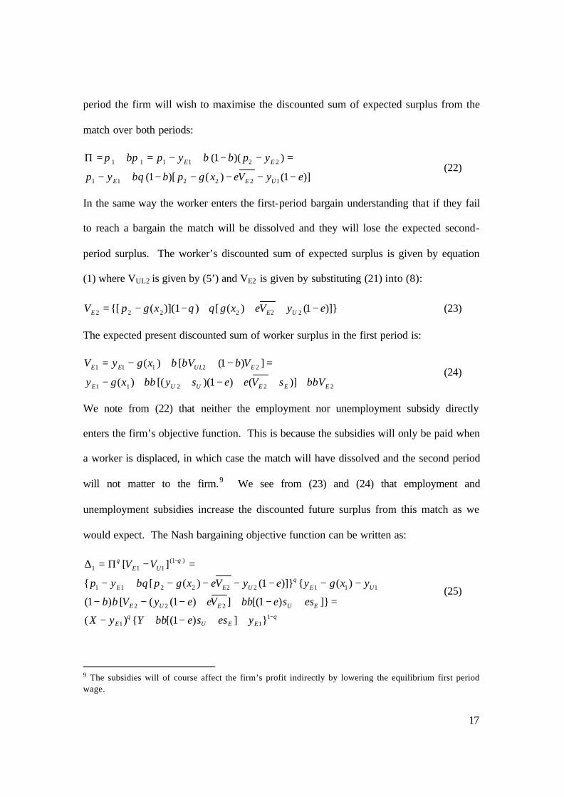
17

period the firm will wish to maximise the discounted sum of expected surplus from the

match over both periods:

)]1()()[1(

))(1(

122211

221111

eyVexgpbyp

ypbyp

UEE

EE

−−−−−+−

=−−+−=+=Π

βθ

ββππ (22)

In the same way the worker enters the first-period bargain understanding that if they fail

to reach a bargain the match will be dissolved and they will lose the expected second-

period surplus. The worker’s discounted sum of expected surplus is given by equation

(1) where VUL2 is given by (5’) and VE2 is given by substituting (21) into (8):

)]}1()([)1)](({[ 222222 eyVexgxgpV UEE −+++−−= θθ (23)

The expected present discounted sum of worker surplus in the first period is:

22211

22111

)]()1)([()(

])1([)(

EEEUUE

EULEE

VbsVeesybxgy

VbbVxgyV

ββ

β

+++−++−

=−++−= (24)

We note from (22) that neither the employment nor unemployment subsidy directly

enters the firm’s objective function. This is because the subsidies will only be paid when

a worker is displaced, in which case the match will have dissolved and the second period

will not matter to the firm.9 We see from (23) and (24) that employment and

unemployment subsidies increase the discounted future surplus from this match as we

would expect. The Nash bargaining objective function can be written as:

θθ

θ

θθ

β

ββ

βθ

−

−

++−+−

=+−++−−−

+−−−−−−+−

=−Π=∆

111

222

111222211

)1(111

}])1[({)(

]})1[(])1(([)1(

)({)]}1()([{

][

EEUE

EUEUE

UEUEE

UE

yessebYyX

essebVeeyVb

yxgyeyVexgpyp

VV

(25)

9 The subsidies will of course affect the firm’s profit indirectly by lowering the equilibrium first period wage.

18

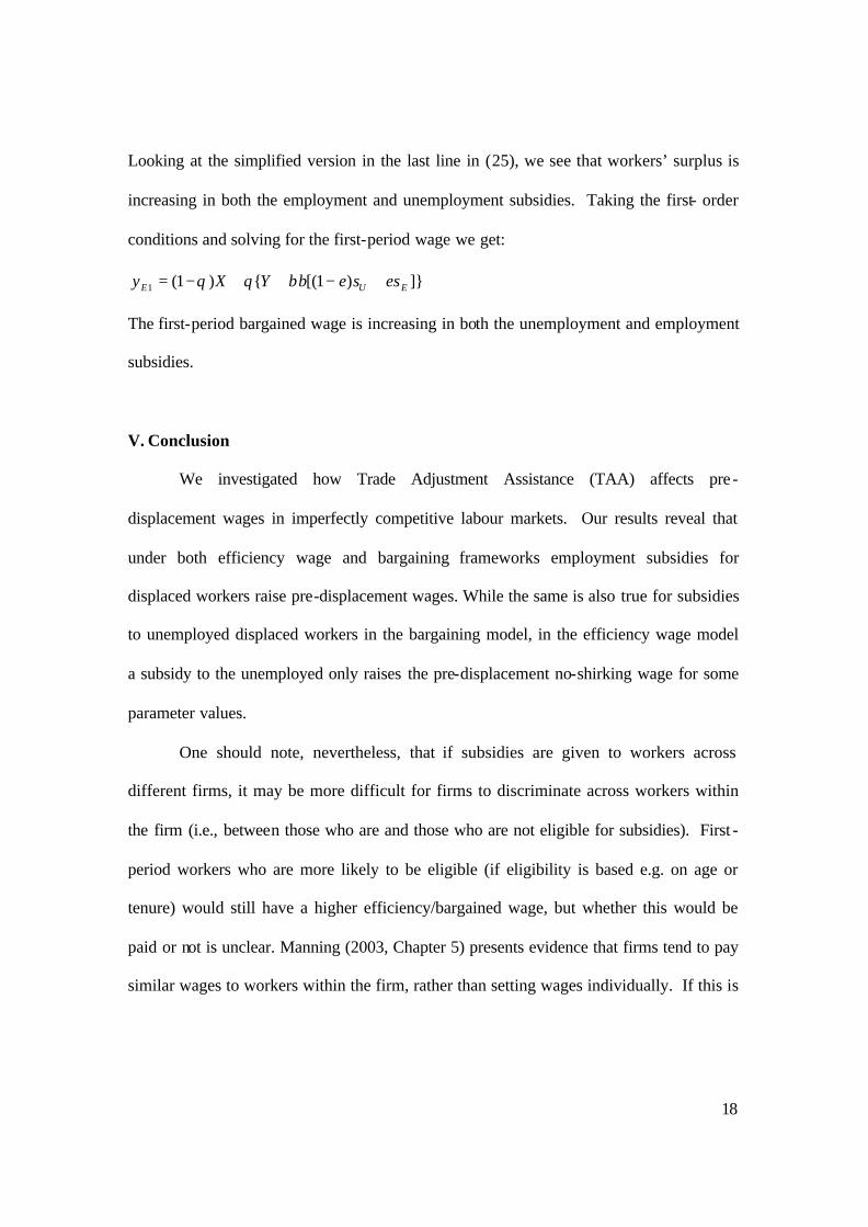
Looking at the simplified version in the last line in (25), we see that workers’ surplus is

increasing in both the employment and unemployment subsidies. Taking the first- order

conditions and solving for the first-period wage we get:

]})1[({)1(1 EUE essebYXy +−++−= βθθ

The first-period bargained wage is increasing in both the unemployment and employment

subsidies.

V. Conclusion

We investigated how Trade Adjustment Assistance (TAA) affects pre -

displacement wages in imperfectly competitive labour markets. Our results reveal that

under both efficiency wage and bargaining frameworks employment subsidies for

displaced workers raise pre-displacement wages. While the same is also true for subsidies

to unemployed displaced workers in the bargaining model, in the efficiency wage model

a subsidy to the unemployed only raises the pre-displacement no-shirking wage for some

parameter values.

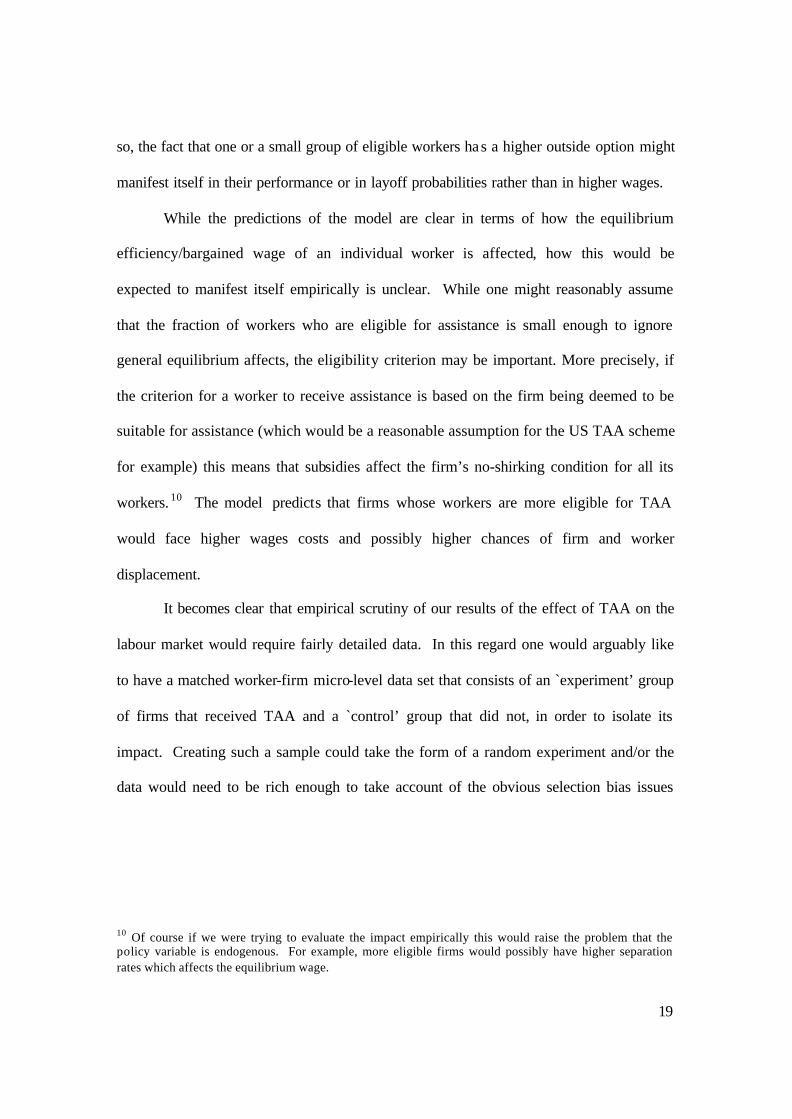
One should note, nevertheless, that if subsidies are given to workers across

different firms, it may be more difficult for firms to discriminate across workers within

the firm (i.e., between those who are and those who are not eligible for subsidies). First -

period workers who are more likely to be eligible (if eligibility is based e.g. on age or

tenure) would still have a higher efficiency/bargained wage, but whether this would be

paid or not is unclear. Manning (2003, Chapter 5) presents evidence that firms tend to pay

similar wages to workers within the firm, rather than setting wages individually. If this is

19

so, the fact that one or a small group of eligible workers has a higher outside option might

manifest itself in their performance or in layoff probabilities rather than in higher wages.

While the predictions of the model are clear in terms of how the equilibrium

efficiency/bargained wage of an individual worker is affected, how this would be

expected to manifest itself empirically is unclear. While one might reasonably assume

that the fraction of workers who are eligible for assistance is small enough to ignore

general equilibrium affects, the eligibility criterion may be important. More precisely, if

the criterion for a worker to receive assistance is based on the firm being deemed to be

suitable for assistance (which would be a reasonable assumption for the US TAA scheme

for example) this means that subsidies affect the firm’s no-shirking condition for all its

workers. 10 The model predicts that firms whose workers are more eligible for TAA

would face higher wages costs and possibly higher chances of firm and worker

displacement.

It becomes clear that empirical scrutiny of our results of the effect of TAA on the

labour market would require fairly detailed data. In this regard one would arguably like

to have a matched worker-firm micro-level data set that consists of an `experiment’ group

of firms that received TAA and a `control’ group that did not, in order to isolate its

impact. Creating such a sample could take the form of a random experiment and/or the

data would need to be rich enough to take account of the obvious selection bias issues

10 Of course if we were trying to evaluate the impact empirically this would raise the problem that the policy variable is endogenous. For example, more eligible firms would possibly have higher separation rates which affects the equilibrium wage.

20

involved in assessing the effect of TAA. As far as we aware, no such detailed data

currently exist.11

11 The paucity of appropriate data for supportive empirical evidence of the effect of TAA becomes obvious from the literature review provided by Baicker and Rehavi (2004). In their discussion of empirical evidence of its effects the authors are only able to resort to secondary evidence by referring to the literature on the impact of changes in unemployment insurance on the labour market. However, as they themselves note, “applying evidence from unemployed workers in general to workers receiving trade adjustment is problematic, since TAA workers have different employment and demographic profiles from the average unemp loyed worker” (p. 249).

21

References Baicker, Katherine and Rehavi, M. Marit (2004), “Trade Adjustment Assistance”, Journal of Economic Perspectives , Vol. 18, No. 2 Spring, pp239-55. Barry, F. (1995) "Declining High-Wage Industries, Efficient Labour Contracts and Optimal Adjustment Assistance", Canadian Journal of Economics, 28, 94-107, 1995. Blanchflower, David G. and Andrew J. Oswald (2005), “The Wage Curve Reloaded” NBER working paper number 11338. Bloom, H., S. Schwartz, S. Lui-Gurr and S.W. Lee (1999) “Testing a Re-employment Incentive for Displaced Workers: The Earnings Supplement Project” Social Research and Demonstration Corporation, New York University Booth, Alison (1995). The Economics of the Trade Union. Cambridge University Press. Brecher, R., and E. Choudri (1994) “Pareto Gains from Trade, Reconsidered: Compensating for Jobs Lost,” Journal of International Economics 36 (May 1994), 223–38. Breen, Richard and Halpin, B. (1989), Subsidising Jobs: An Evaluation of the Employment Incentive Schemes, General Research Series 144, Economic and Social Research Institute, Dublin Davidson, Carl and Steven J. Matusz (2005) “Trade Liberalization and Compensation”, Forthcoming, International Economic Review Dixit, A., and V. Norman (1986) “Gains from Trade without Lump-Sum Compensation,” Journal of International Economics 21, 111–22. Feenstra, R., and T. Lewis (1994) “Trade Adjustment Assistance and Pareto Gains from Trade,” Journal of International Economics 36, 201–22. Kandori, M. (1992) “Repeated games played by overlapping generations of players”, Review of Economic Studies, 59 (1), pp81-92 Kletzer, Lori G. (2004) “Trade-related Job Loss and Wage insurance: a Synthetic Review” Review of International Economics, 12 (5), 724-748. Kletzer, L. and R. Litan (2001), “A Prescription to Relieve Worker Anxiety,” Policy Brief No. 73 (Washington, DC: Brookings Institution). Manning, A. (2003). Monopsony in Motion, Imperfect Competition in Labor Markets, Princeton University Press

22

Oswald, Andrew J. (1993). “Efficient Contracts are on the Labour Demand Curve” Labour Economics , Vol 1, pp 85-113. Pissarides, Christopher A. (2000) “Equilibrium Unemployment Theory” 2nd ed., Cambridge MA: MIT Press. Scheve, F. K., and M. Slaughter (2001) Globalization and the Perception of American Workers (Washington, DC: Institute for International Economics). Shapiro, C. and Joseph Stiglitz (1984) “Equilibrium Unemployment as a Worker Discipline Device” American Economic Review, June 433-444

23

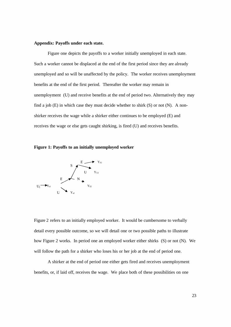
Appendix: Payoffs under each state.

Figure one depicts the payoffs to a worker initially unemployed in each state.

Such a worker cannot be displaced at the end of the first period since they are already

unemployed and so will be unaffected by the policy. The worker receives unemployment

benefits at the end of the first period. Thereafter the worker may remain in

unemployment (U) and receive benefits at the end of period two. Alternatively they may

find a job (E) in which case they must decide whether to shirk (S) or not (N). A non-

shirker receives the wage while a shirker either continues to be employed (E) and

receives the wage or else gets caught shirking, is fired (U) and receives benefits.

Figure 1: Payoffs to an initially unemployed worker

Figure 2 refers to an initially employed worker. It would be cumbersome to verbally

detail every possible outcome, so we will detail one or two possible paths to illustrate

how Figure 2 works. In period one an employed worker either shirks (S) or not (N). We

will follow the path for a shirker who loses his or her job at the end of period one.

A shirker at the end of period one either gets fired and receives unemployment

benefits, or, if laid off, receives the wage. We place both of these possibilities on one

S

E

Yu1

N

E

U1

U Yu2

YE2

YE2

U YU2

24

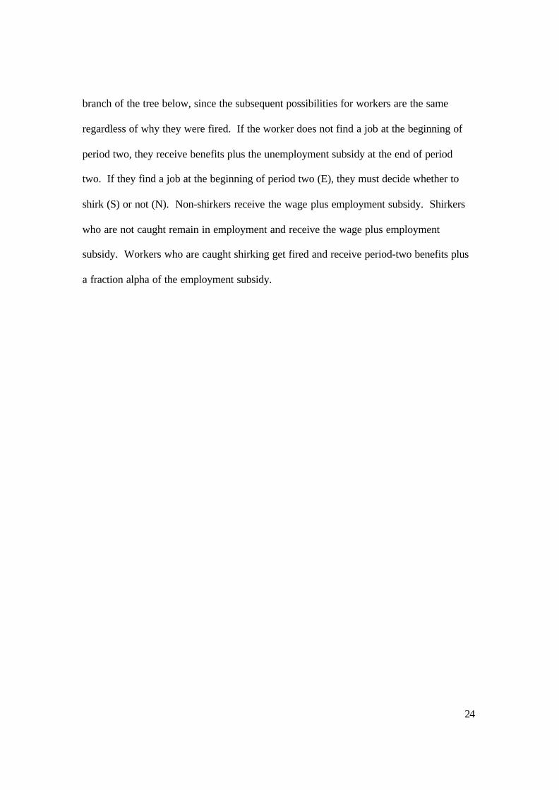
branch of the tree below, since the subsequent possibilities for workers are the same

regardless of why they were fired. If the worker does not find a job at the beginning of

period two, they receive benefits plus the unemployment subsidy at the end of period

two. If they find a job at the beginning of period two (E), they must decide whether to

shirk (S) or not (N). Non-shirkers receive the wage plus employment subsidy. Shirkers

who are not caught remain in employment and receive the wage plus employment

subsidy. Workers who are caught shirking get fired and receive period-two benefits plus

a fraction alpha of the employment subsidy.

25

Figure 2: Payoffs to an initially employed worker

YE1

S

E

U

YU1 YE1

S

N

E1

E

U

YE2

YE2

YU2+eSu

NYE1

YE1

E

U

E

U

S

NYU2 +Su YEL2+SE

E

U

YEL2+SE

YU2+aSE

U

S

NE

UYE2

YE2

YU2 +Su

E

S

NYEL2+SE

E

U

YEL2+SE

YU2+aSE

YU2+eSu

26