Dissertations and Theses

12-2016

Traction and Launch Control for a Rear-Wheel-Drive Parallel-Series Traction and Launch Control for a Rear-Wheel-Drive Parallel-Series

Plug-In Hybrid Electric Vehicle Plug-In Hybrid Electric Vehicle

Adam Michael Szechy

Follow this and additional works at: https://commons.erau.edu/edt

Part of the Automotive Engineering Commons, and the Mechanical Engineering Commons

Scholarly Commons Citation Scholarly Commons Citation Szechy, Adam Michael, "Traction and Launch Control for a Rear-Wheel-Drive Parallel-Series Plug-In Hybrid Electric Vehicle" (2016). Dissertations and Theses. 315. https://commons.erau.edu/edt/315

This Thesis - Open Access is brought to you for free and open access by Scholarly Commons. It has been accepted for inclusion in Dissertations and Theses by an authorized administrator of Scholarly Commons. For more information, please contact commons@erau.edu.

TRACTION AND LAUNCH CONTROL FOR A REAR-WHEEL-DRIVE PARALLEL-

SERIES PLUG-IN HYBRID ELECTRIC VEHICLE

by

Adam Michael Szechy

A Thesis Submitted to the College of Engineering Department of Mechanical

Engineering in Partial Fulfillment of the Requirements for the Degree of

Master of Science in Mechanical Engineering

Embry-Riddle Aeronautical University

Daytona Beach, Florida

December 2016

ii

Acknowledgements

I would like to thank my thesis advisor Dr. Patrick Currier for providing the

guidance and support to complete this research.

I would like to thank my teammates Dylan Lewton, Matthew Nelson, Abdulla

Karmustaji, Rohit Gulati on the Embry-Riddle EcoCAR 3 team that helped develop the

initial powertrain model that was used during architecture selection for the competition. I

would like to thank Dr. Marc Compere for the base six degree of freedom vehicle

dynamics model that was developed in his Advanced Vehicle Dynamics class at Embry-

Riddle.

I would also like to thank the EcoCAR 3 competition for providing this vehicle

and unique competition to do my research on.

iii

Abstract

Researcher: Adam Michael Szechy

Title: Traction and Launch Control for a Rear-Wheel-Drive Parallel-Series Plug-

in Hybrid Electric Vehicle

Institution: Embry-Riddle Aeronautical University

Degree: Master of Science in Mechanical Engineering

Year: 2016

Hybrid vehicles are becoming the future of automobiles leading into the all-electric

generation of vehicles. Electric vehicles come with a great increase in torque at lower

RPM resulting in the issue of transferring this torque to the ground effectively. In this

thesis, a method is presented for limiting wheel slip and targeting the ideal slip ratio for

dry asphalt and low friction surfaces at every given time step. A launch control system is

developed to further reduce wheel slip on initial acceleration from standstill furthering

acceleration rates to sixty miles per hour. A MATLAB Simulink model was built of the

powertrain as well as a six degree of freedom vehicle model that has been validated with

real testing data from the car. This model was utilized to provide a reliable platform for

optimizing control strategies without having to have access to the physical vehicle, thus

reducing physical testing. A nine percent increase has been achieved by utilizing traction

control and launch control for initial vehicle movement to sixty miles per hour.

iv

Table of Contents Thesis Review Committee ................................................................................................... i

Acknowledgements ............................................................................................................. ii

Abstract .............................................................................................................................. iii

List of Tables ..................................................................................................................... vi

List of Figures ................................................................................................................... vii

List of Acronyms ............................................................................................................... ix

Introduction ................................................................................................................. 1

Significance of the Study ........................................................................................ 1

Statement of the Problem ........................................................................................ 2

Limitations and Assumptions ................................................................................. 2

Vehicle Architecture ............................................................................................... 3

Thesis Statement ..................................................................................................... 5

Review of the Relevant Literature ............................................................................... 6

Hybrid Vehicle Modeling ....................................................................................... 6

Traction Control Systems ....................................................................................... 6

Launch Control ....................................................................................................... 9

Tire-Road Friction Estimation ................................................................................ 9

Slip Ratio .............................................................................................................. 11

Methodology .............................................................................................................. 12

Powertrain Model Development ........................................................................... 12

Vehicle Body Model Development ...................................................................... 17

Traction Control .................................................................................................... 19

Launch Control ..................................................................................................... 24

Vehicle Testing ..................................................................................................... 28

Results ....................................................................................................................... 30

Model Validation .................................................................................................. 30

Traction Control Dry Asphalt ............................................................................... 33

Traction Control Split Mu ..................................................................................... 36

Launch Control ..................................................................................................... 41

Conclusions, and Future Work .................................................................................. 47

Conclusions ........................................................................................................... 47

Future Work .......................................................................................................... 48

Appendix ........................................................................................................................... 49

v

Bibliography ..................................................................................................................... 49

vi

List of Tables Table 1: IVM to sixty times on dry asphalt 32

Table 2: IVM to sixty times on split mu 36

Table 3: Generator set and traction motor initial launch RPM compared to IVM-30 43

Table 4: Modeled launch control compared to no current offset 45

vii

List of Figures Figure 1: Torque comparison between an internal combustion engine and electric

machine 1

Figure 2: Power comparison between an internal combustion engine and electric machine

2

Figure 3: Selected architecture diagram 4

Figure 4: Power flow diagram for different operating modes 4

Figure 5: GM LEA Model 13

Figure 6: Simulink to Simscape physical system 13

Figure 7: Bosch IMG model 14

Figure 8: Clutch model 15

Figure 9: Powertrain to vehicle body transition 16

Figure 10: A123 battery model 17

Figure 11: Usable power calculation 20

Figure 12: Torque split logic 21

Figure 13: Traction control torque intervention block diagram 23

Figure 14: Active brake control block diagram 24

Figure 15: Launch control Stateflow 26

Figure 16: Generator set speed controller block diagram 27

Figure 17: Traction motor speed controller block diagram 27

Figure 18: Engine torque controller block diagram 28

Figure 19: TRC velocity data compared to vehicle body model 30

Figure 20: TRC wheel slip compared to vehicle body model 31

Figure 21: Modeled vehicle speed compared to rear wheel speeds without interventions33

Figure 22: Model vehicle speed compared to rear wheel speeds for torque reduction 34

Figure 23: Modeled torque reductions compared to wheel slip 35

Figure 24: Torque reduction compared to wheel slip on vehicle 35

Figure 25: Modeled vehicle speed compared to rear wheel speeds for torque reductions

and active brake control 36

Figure 26: Modeled vehicle speed compared to rear wheel speeds without interventions

on split mu 37

Figure 27: Vehicle course on split mu without interventions 37

Figure 28: Modeled vehicle speed compared to rear wheel speeds for torque reduction on

split mu 38

Figure 29: Vehicle course on split mu with torque reduction 39

Figure 30: Longitudinal tire forces on split mu during torque interventions 39

viii

Figure 31: Modeled vehicle speed compared to rear wheel speeds for torque reduction

and active brake control on split mu 40

Figure 32: Vehicle course on split mu with torque reduction and active brake control 40

Figure 33: Modeled launch control IVM-30 generator set vs traction motor RPM 41

Figure 34: On vehicle launch control clutch engagement with gradual throttle application

42

Figure 35: Model launch control with the engine offsetting the HV bus current draw 44

Figure 36: Modeled launch control without the engine offsetting the HV bus current draw

44

Figure 37: On vehicle launch control clutch engagement with full throttle application 45

Figure 38: On vehicle launch control total torque with TCS torque reductions 46

ix

List of Acronyms

BMS Battery management system

CAN Controlled area network

EM Electric machine

ICE Internal combustion engine

IMG Integrated motor generator

IVM Initial vehicle movement

PHEV Plug-in hybrid electric vehicle

RWD Rear-wheel-drive

TCS Traction control system

1

Chapter I

Introduction

Significance of the Study

Hybrid vehicles and all electric vehicles are becoming the future of the

automobile industry. In countries such as Germany by 2030 sales of internal combustion

engine automobiles are to be banned (Fingas, 2016). From there on all vehicles have to

be zero-emissions, either electric or hydrogen. Forcing auto manufactures to focus on

hybridization of automobiles followed by the complete switch to all electric. By

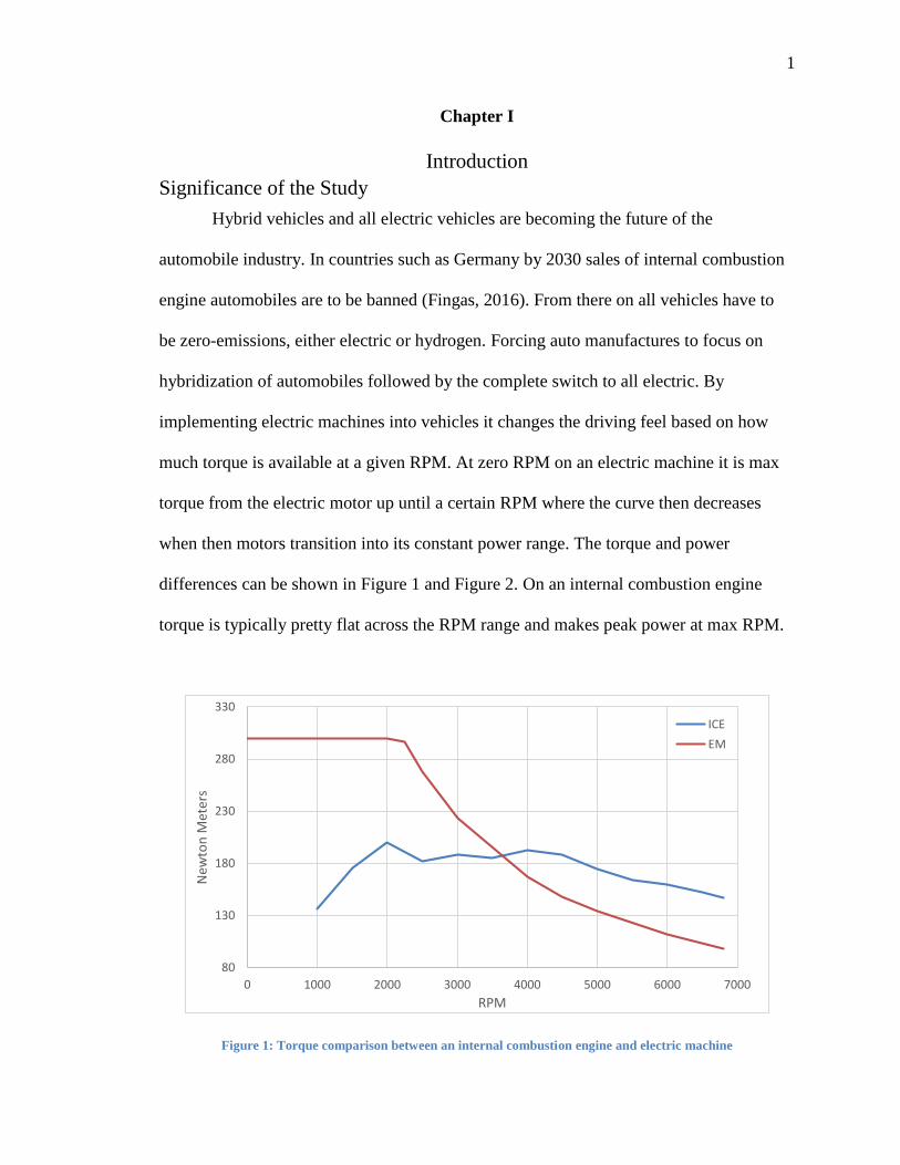
implementing electric machines into vehicles it changes the driving feel based on how

much torque is available at a given RPM. At zero RPM on an electric machine it is max

torque from the electric motor up until a certain RPM where the curve then decreases

when then motors transition into its constant power range. The torque and power

differences can be shown in Figure 1 and Figure 2. On an internal combustion engine

torque is typically pretty flat across the RPM range and makes peak power at max RPM.

Figure 1: Torque comparison between an internal combustion engine and electric machine

80

130

180

230

280

330

0 1000 2000 3000 4000 5000 6000 7000

New

ton

Met

ers

RPM

ICE

EM

2

Figure 2: Power comparison between an internal combustion engine and electric machine

Due the greater amount of torque on the lower range of the RPM curve it is

important to be able to get the torque delivered to the ground as safely and efficiently as

possible by mitigating the amount of wheel slip.

Statement of the Problem

Under hard acceleration with a parallel-series hybrid vehicle with an automatic

transmission, a high amount of torque is available at low RPM thus the driven wheels

experience a high amount of slip from a standstill. The amount of torque needs to be

regulated to limit the amount of slip to deliver the smoothest and fastest acceleration

possible. Also, while driving on various surfaces with different friction coefficients slip is

more prone to happen, thus limiting the wheel slip is needed to keep the vehicle stable.

Limitations and Assumptions

Pacejka coefficients from generic tires

Damping effects during weight transfer

0

20

40

60

80

100

120

0 1000 2000 3000 4000 5000 6000 7000

Kilo

wat

ts

RPM

ICE

EM

3

Constant electric machine temperatures

Torque converter clutch is always locked

Wheels are pointed straight ahead

Vehicle Architecture

The architecture of the vehicle for this study was developed for the EcoCAR 3

competition. The competition is put on by Argonne National Labs and the Department of

Energy. The vehicle, a 2016 Chevrolet Camaro, was donated by General Motors. The

goal of the competition is to reduce the environmental impact while keeping the expected

performance of the iconic car. There is a total of 16 universities competing in this

competition in North America all with different architectures.

The select architecture is a parallel-series utilizing a GM LEA Ecotec internal

combustion engine and two Bosch IMG electric motors. The LEA engine is coupled to a

hydraulic clutch followed by the Bosch IMG. This IMG is followed by another clutch

and IMG which is feed into a 8L90 eight speed automatic transmission with a torque

converter. This architecture is shown in Figure 3. The IMG coupled to the LEA is

referred to as the generator motor, whereas the IMG coupled to the transmission is

referred to as the traction motor. When the clutch between the generator and traction

motor is open it allows the vehicle to run in a series configuration. This allows the LEA

to run and generate power through the generator motor at its most efficient operating

points while being decoupled from the road. When the clutch between the generator and

traction motor is closed it allows the vehicle to run as a parallel configuration. This gives

the potential for the LEA, generator motor, and traction motor to send torque to the rear

wheels. The various operating modes are shown in Figure 4.

4

Figure 3: Selected architecture diagram

Figure 4: Power flow diagram for different operating modes

5

In parallel charge deplete mode the LEA will be the only torque producing

component send torque to the rear wheels, while the generator motor applies additional

load to the LEA to make the current draw on the high voltage bus zero to offset the

accessory loads of the vehicle. For sports mode all torque producing components send

torque to the rear wheels.

Thesis Statement

Traction control and launch control using a tire force observer to regulate electric

motor torque can significantly reduce acceleration times from IVM-60 in hybrid electric

vehicles in both standard and split mu conditions.

6

Chapter II

Review of the Relevant Literature

Hybrid Vehicle Modeling

To model performance of a vehicle architectures and control strategies Simulink

is used. This is done by modeling each component of the hybrid vehicle using a first-

principles approach and validated by experimental data. These components are then

constructed into a coupled nonlinear dynamic model. A supervisory controller is then

programmed to optimized the energy flow in the powertrain. The simulation yields the

results of vehicle behavior and component energy losses (Evangelou & Shabbir, 2016).

In a front-engine, rear-wheel-drive car the rear wheels have a normal force change

due to the drive torque. The driveshaft torque has to be counteracted by a change in the

rear wheel loads with the left tire increasing and right tire decreasing. The change has to

be solved to take in account the torque is being reacted by the front engine mounts

(Milliken & Milliken, 1995). The drive torque reaction at the engine and transmission is

transferred in a distribution between the front and rear suspension. Typically, the roll

torque produced by the suspension is proportional to the roll angle of the chassis

(Gillespie, 1992).

Traction Control Systems

Traction control is implemented by changing gears to reduce driving torque on the

driven wheels and manipulating throttle position. A road coefficient estimator determines

the friction coefficient of the road; from there the driving torque is determined by the slip

controller. An optimal throttle position and gear can then be determined. Simulations

show this algorithm improves vehicle acceleration on various road conditions (Shi, Li,

Lu, & Zhang, 2012).

7

Another approach of implementing fuzzy controller for TCS due to PID

controllers cannot meet the requirements in complicated road conditions. A fuzzy PID

controller is used to regulate the engine torque. The active brakes are driven by a sliding

mode controller. When the driving force exceeds the friction force the wheel begins to

slip. TCS then estimates the optimal slip ratio, then engine controller and brake controller

then adjust output to meet this target. On low friction surface engine torque is regulate to

maintain the optimal slip. In a split mu condition the engine torque is regulated as well as

the brake controller. The driving wheels are regulated by the brake controller and the

engine output torque is increased (Liu & Jin, 2016).

For abrupt changes in road friction a PID and fuzzy controller are used to

regulate the driving torque. The PID controller calculate the base torque for TCS and

fuzzy controller calculates the compensating factor for the change in friction. Simulations

have proven that the controller is robust and effective, compared to conventional PID

controller the performance is improved greatly (Li, et al., 2012).

Sliding-mode controllers can be used to determine the estimated max friction to

determine the maximum torque for the wheels based on a LuGre friction model. A

sliding-mode control was utilized due to the nonlinear system (Kuntanapreeda, Traction

Control of Electric Vehicles Using Sliding-Mode Controller with Tractive Force

Observer, 2014).

When utilizing brake control for traction control there are different strategies for

resetting the control to get optimal results. By using reset control with zero crossing,

fixed reset bands, and variable reset bands the output to the system improves transient

8

time and overshooting. The system is very robust and adheres to changes in friction

conditions (Cerdeira-Corujo, Costas, Delgado, & Barreiro, 2016).

A super-twisting algorithm was implemented as a traction controller for road

vehicles. Control targets a desired wheel slip ratio by using a super-twisting based

sliding-mode control law and a nonlinearity observer. Controller was able to meet the

desired slip target even under changes in road friction. This controller has shown to have

better performance than a conventional sliding-mode controller (Kuntanapreeda, Super-

twisting sliding-mode traction control of vehicles with tractive force observer, 2015).

Formula 1 traction control uses a PID closed-loop feedback control with an

advanced fuel cutoff algorithm. Torque reductions can be done by reducing throttle

position, ignition retard, or switching off ignition or fuel injection to a number of

cylinders. Ignition retardation was found to elevate the exhaust valve to potential failure

point. Ignition cuts were found to was fuel, so fuel cuts were determined to be the best

implementation. Wheel slip is calculated by reference speed of the vehicle, in this case

the maximum value of the two front wheels. The desired slip ratio is calculated based on

car speed, throttle position, gear position and the current lateral acceleration (Lyon,

Philipp, & Grommes, 1994).

Motorcycle traction control is used to improve dynamic performance using

artificial neural networks and fuzzy logic. The neural network is used determine the

optimal slip ratio based on the surface of the road. The fuzzy logic calculates the desired

throttle positon based on the optimal slip ratio (Urda, Cabrera, Castillo, & Guerra, 2015).

Another approach of using a second-order sliding mode controller with a nonlinear

9

dynamic model of rear wheel slip. Torque reductions are performed by changing the

throttle body valve position (Tanelli, Vecchio, Corno, Ferrara, & Savaresi, 2009).

Launch Control

The launch controller manages the acceleration phase of the vehicle by utilizing

the clutch of the transmission. On a sports bike an electronic hydraulic clutch was utilized

to control the clutch engagement. First the bike is toggled into launch control mode and

the clutch is fully disengaged, once shifted into first gear the clutch targets the kiss point

at which it starts grabbing. As throttle is increase the clutch is feathered in giving the

desired acceleration rate, to maintain on this ideal acceleration the can be commanded to

slip more if necessary (Giani, Tanelli, Savaresi, & Santucci, 2013).

Some vehicles use electronically controlled variable transmissions which contain

a planetary gear set, this allows the engine to run at a different speed than the wheels. The

controller provides a counter torque at the wheels to cancel out the torque at the engine

with an electric motor. On conventional vehicles the brake can be applied and torque is

transferred through the torque converter to the wheels as engine RPM is increased. The

standard launch control features cannot be utilized in hybrid vehicles (NewsRx, 2015).

Using a spark retard to limit the internal combustion engine RPM while the driver

is at 100 percent throttle. This also allows for easy rev matching during shifting to unload

the transmission during shifts. A controller is a PID for the spark retardation to reduce

engine power during traction limitations (Delarammatikas, 2011).

Tire-Road Friction Estimation

Estimation of individual wheel friction coefficients to the road are estimated by

slip ratios and longitudinal tire forces. This is achieved by using a recursive least-squares

10

parameter identification. The observer uses engine torque, brake torque, and an

accelerometer (Rajamani, Phanomchoeng, Piyabongkarn, & Lew, 2012).

Instantaneous friction and lateral forces can be computed from filtering noisy

signals from the vehicle. A braking stiffness concept is used to determine the road type

when braking. Utilizing a Dugoff model to estimate the maximum friction coefficient,

producing promising results in noisy experimentations (Villagra, 2010).

The vehicle controller requires a good knowledge of the interaction of tires to the

road. To do so an estimation of the tire to road parameters are evaluated in real-time.

This is done using a trust-region based method to determine the friction parameters. A

LuGre model-based nonlinear least squares parameter estimation is used in conjunction

with vehicle dynamics data from the vehicle in real-time. Promising results have been

obtained in simulations for all road surfaces (Sharifzadeh, Akbari, Timpone, & Daryani,

2016).

Measuring tire-road friction coefficient is hard without expensive equipment. A

method using auxiliary particle filter and iterated extended kalman filter is implemented.

The filters are used to estimate the slip angles of the front tires, which can be used to

determine a preliminary sideslip angle. The iterated extended kalman filter is used to

make the estimation of the sideslip angle for accurate. The iteration algorithm is used to

estimate the friction based on the self-aligning torque of the wheels. The self-aligning

torque is more sensitive to tire slip which provides faster estimation. Using simulations

and vehicle testing in winter gave validation to this method as well as efficiency (Liu, Li,

Yang, Ji, & Wu, 2017).

11

With cars moving to electric power steering it allows for another method to

estimate the tire-road friction coefficient. By utilizing the steering torque measurements

in real-time the self-aligning torques can be estimated. A study of using a lumped axle

assumption shows poor results for front axle force values compared to using independent

wheels (Beal, 2016).

Slip Ratio

Change in tire pressure can impact the optimal slip ratio. Utilizing a second-order

factor an improved prediction for slip ratio can be determined. The change in tire

pressure changes the longitudinal slip stiffness as well as the peak friction coefficient.

Results show under braking with different tire pressures stopping distances and times are

shortened with the improved prediction (Li, Wang, Zhang, Gu, & Shen, 2015).

12

Chapter III

Methodology

Powertrain Model Development

To conduct this research a powertrain model is need to develop a traction control

system and launch control. The powertrain model was created utilizing Mathworks

Simulink which is comprised of mostly Simscape to model the physical systems. It is

composed of a GM LEA engine, two Bosch IMG motors, two hydraulic clutches, GM

8L90 transmission, differential, and a A123 battery. The signals sent and received from

the powertrain to the controller are simulated through Vector Virtual CAN channels to

get the signal delay and sample rate to match the physical hardware.

The GM LEA engine is composed of lookup tables of torque curves vs intake port

flow and RPM. The model is shown in Figure 5. A Simscape model of the intake and

throttle body drives the torque look up table, the torque output is fed into a Simscape

ideal torque sensor. The engine RPM is read off the physical system by a Simscape ideal

rotational motion sensor shown in Figure 6. The proper inertia of the engine is set on the

engine to give the proper acceleration and deceleration of the engine. By utilizing real

data from the components through lookup tables the physical system can be modeled

accurately by implementing inertias, also the intake the ambient air temperature and

pressure can be varied altering the performance. This allows direct comparisons between

the model system and testing performed on the vehicle based on ambient conditions.

13

Figure 5: GM LEA Model

Figure 6: Simulink to Simscape physical system

The Bosch IMG models are constructed of lookup tables for torque based on

voltage and RPM, as well as efficiencies based on torque and RPM. The torque output is

fed into a Simscape ideal torque sensor; the RPM is read off the physical system by a

Simscape ideal rotational motion sensor. The desired torque is saturated by the max

available torque from the motoring and regen torque lookup tables. The efficiencies are

14

used to calculate the current draw on the high voltage bus. The model can be seen in

Figure 7. The limitations of the model are that the efficiencies do not correlate to a

temperature increase of the motor itself, the motors on the physical vehicle will be

automatically de-rated on performance by the inverter based on temperature which is not

accounted for in this model.

Figure 7: Bosch IMG model

The clutches are model in Simscape as a disk friction clutches. The clutches are

normally closed and open at 14 bar of pressure. The Simscape block works by applying

pressure allows the transfer of torque so a lookup table is used to flip the logic. The

clutch model can be seen in Figure 8. The physical properties of the clutch can be

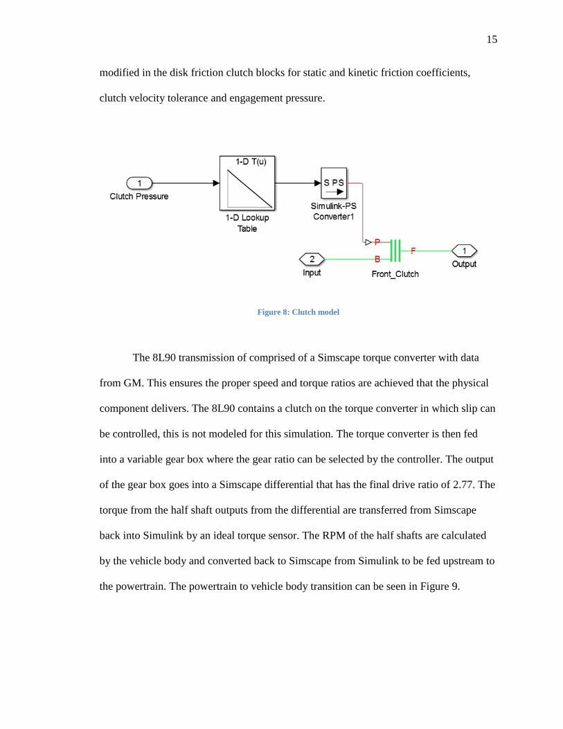
15

modified in the disk friction clutch blocks for static and kinetic friction coefficients,

clutch velocity tolerance and engagement pressure.

Figure 8: Clutch model

The 8L90 transmission of comprised of a Simscape torque converter with data

from GM. This ensures the proper speed and torque ratios are achieved that the physical

component delivers. The 8L90 contains a clutch on the torque converter in which slip can

be controlled, this is not modeled for this simulation. The torque converter is then fed

into a variable gear box where the gear ratio can be selected by the controller. The output

of the gear box goes into a Simscape differential that has the final drive ratio of 2.77. The

torque from the half shaft outputs from the differential are transferred from Simscape

back into Simulink by an ideal torque sensor. The RPM of the half shafts are calculated

by the vehicle body and converted back to Simscape from Simulink to be fed upstream to

the powertrain. The powertrain to vehicle body transition can be seen in Figure 9.

16

Figure 9: Powertrain to vehicle body transition

The A123 battery pack is based on a lookup table for voltage with current draw

from physical testing. The internal resistance varies with temperature and state of charge

with is supplied from the manufacturer. The internal resistance drives the battery thermal

model. A phase change material is also modeled to cool the battery pack. The soft ECU

of the battery model utilizes lookup tables from the manufacturer for max charge and

discharge power and current for continuous use and 10 second bursts based on these

temperature and state of charge. The current is averaged for the last 10 seconds and

divided by the max discharge current to get the percentage of the buffer left. This

increases the fidelity of battery model by having its performance characteristics change

with these factors. The battery model can be seen in Figure 10.

17

Figure 10: A123 battery model

Vehicle Body Model Development

A six degree of freedom model was implemented that consists of axle subsystems

were wheel angular velocities are first calculated.

𝛺 = ∫𝜏𝑡𝑟𝑎𝑐𝑡𝑖𝑣𝑒 − (𝐹𝑥𝑟𝑑𝑦𝑚) − 𝐹𝑟𝑜𝑎𝑑 𝑙𝑜𝑎𝑑 − 𝜏𝑏𝑟𝑎𝑘𝑒

𝑟𝑜𝑡𝑎𝑡𝑖𝑜𝑛𝑎𝑙 𝑖𝑛𝑒𝑟𝑡𝑖𝑎

Where:

𝜏𝑡𝑟𝑎𝑐𝑡𝑖𝑣𝑒 = 𝑡𝑜𝑟𝑞𝑢𝑒 𝑓𝑟𝑜𝑚 𝑝𝑜𝑤𝑒𝑟𝑡𝑟𝑎𝑖𝑛

𝜏𝑏𝑟𝑎𝑘𝑒 = 𝑡𝑜𝑟𝑞𝑢𝑒 𝑓𝑜𝑟𝑚 𝑏𝑟𝑎𝑘𝑒𝑠

𝐹𝑥 = 𝑙𝑜𝑛𝑔𝑖𝑡𝑢𝑑𝑖𝑛𝑎𝑙 𝑓𝑜𝑟𝑐𝑒 𝑓𝑟𝑜𝑚 𝑝𝑎𝑐𝑒𝑗𝑘𝑎 𝑡𝑖𝑟𝑒 𝑚𝑜𝑑𝑒𝑙

𝐹𝑟𝑜𝑎𝑑 𝑙𝑜𝑎𝑑 = 𝑎𝑒𝑟𝑜𝑑𝑦𝑛𝑎𝑚𝑖𝑐 𝑟𝑜𝑎𝑑 𝑙𝑜𝑎𝑑

𝑟𝑑𝑦𝑛 = 𝑑𝑦𝑛𝑎𝑚𝑖𝑐 𝑟𝑜𝑙𝑙𝑜𝑖𝑛𝑔 𝑟𝑎𝑑𝑖𝑢𝑠

Aerodynamic load was taking into consideration for the vehicle model, the

following equation was used based on donated data from GM (Kadijk & Ligterink,

2012).

𝐹𝑟𝑜𝑎𝑑 𝑙𝑜𝑎𝑑 = 𝐹0 + 𝐹1𝜈𝑥 + 𝐹2𝜈𝑥2

18

Where:

𝐹0 = 𝑙𝑏𝑓

𝐹1 = 𝑙𝑏𝑓/𝑚𝑝ℎ

𝐹2 = 𝑙𝑏𝑓/𝑚𝑝ℎ2

The axle angular velocity is then used to calculate the slip ratio of the wheel base

on the longitudinal velocity of the vehicle. Wheel slip is calculated by the following

equation (Robert Bosch GmbH, 2004).

𝜆 =𝜔𝑅𝑟𝑑𝑦𝑛 − 𝜈𝑥

𝜔𝑅𝑟𝑑𝑦𝑛

Where:

𝜔𝑅 = 𝑎𝑛𝑔𝑢𝑙𝑎𝑟 𝑠𝑝𝑒𝑒𝑑 𝑜𝑓 𝑡ℎ𝑒 𝑤ℎ𝑒𝑒𝑙

𝑟𝑑𝑦𝑛 = 𝑑𝑦𝑛𝑎𝑚𝑖𝑐 𝑟𝑜𝑙𝑙𝑖𝑛𝑔 𝑟𝑎𝑑𝑖𝑢𝑠

𝜈𝑥 = 𝑙𝑜𝑛𝑔𝑖𝑡𝑢𝑑𝑖𝑛𝑎𝑙 𝑣𝑒𝑙𝑜𝑐𝑖𝑡𝑦

Longitudinal weight transfer model was implemented to give dynamic tires forces

with acceleration. The change of mass is then added to the static to mass of the rear

corner weights and subtracted from the front corner weights.

∆𝑀𝑎𝑠𝑠 =𝐶𝐺 𝐻𝑒𝑖𝑔ℎ𝑡

𝑊ℎ𝑒𝑒𝑙 𝐵𝑎𝑠𝑒∙ 𝑆𝑢𝑠𝑝𝑒𝑛𝑑𝑒𝑑 𝑀𝑎𝑠𝑠 ∙ 𝐿𝑜𝑛𝑔𝑖𝑡𝑢𝑑𝑖𝑛𝑎𝑙 𝐴𝑐𝑐𝑒𝑙𝑒𝑟𝑎𝑡𝑖𝑜𝑛

19

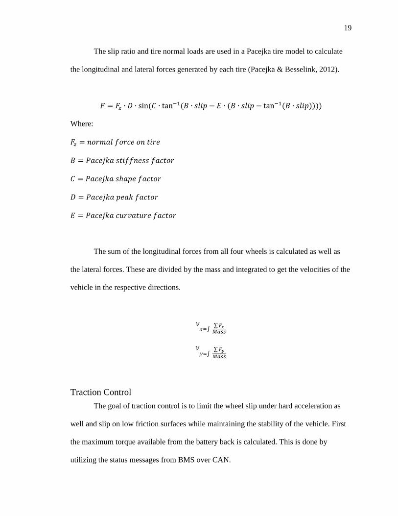
The slip ratio and tire normal loads are used in a Pacejka tire model to calculate

the longitudinal and lateral forces generated by each tire (Pacejka & Besselink, 2012).

𝐹 = 𝐹𝑧 ∙ 𝐷 ∙ sin(𝐶 ∙ tan−1(𝐵 ∙ 𝑠𝑙𝑖𝑝 − 𝐸 ∙ (𝐵 ∙ 𝑠𝑙𝑖𝑝 − tan−1(𝐵 ∙ 𝑠𝑙𝑖𝑝))))

Where:

𝐹𝑧 = 𝑛𝑜𝑟𝑚𝑎𝑙 𝑓𝑜𝑟𝑐𝑒 𝑜𝑛 𝑡𝑖𝑟𝑒

𝐵 = 𝑃𝑎𝑐𝑒𝑗𝑘𝑎 𝑠𝑡𝑖𝑓𝑓𝑛𝑒𝑠𝑠 𝑓𝑎𝑐𝑡𝑜𝑟

𝐶 = 𝑃𝑎𝑐𝑒𝑗𝑘𝑎 𝑠ℎ𝑎𝑝𝑒 𝑓𝑎𝑐𝑡𝑜𝑟

𝐷 = 𝑃𝑎𝑐𝑒𝑗𝑘𝑎 𝑝𝑒𝑎𝑘 𝑓𝑎𝑐𝑡𝑜𝑟

𝐸 = 𝑃𝑎𝑐𝑒𝑗𝑘𝑎 𝑐𝑢𝑟𝑣𝑎𝑡𝑢𝑟𝑒 𝑓𝑎𝑐𝑡𝑜𝑟

The sum of the longitudinal forces from all four wheels is calculated as well as

the lateral forces. These are divided by the mass and integrated to get the velocities of the

vehicle in the respective directions.

𝜈𝑥=∫

∑ 𝐹𝑥𝑀𝑎𝑠𝑠

𝜈𝑦=∫

∑ 𝐹𝑦

𝑀𝑎𝑠𝑠

Traction Control

The goal of traction control is to limit the wheel slip under hard acceleration as

well and slip on low friction surfaces while maintaining the stability of the vehicle. First

the maximum torque available from the battery back is calculated. This is done by

utilizing the status messages from BMS over CAN.

20

𝑃𝑜𝑤𝑒𝑟 (𝑤) = 𝑀𝑎𝑥 𝐷𝑖𝑠𝑐ℎ𝑎𝑟𝑔𝑒 𝐶𝑢𝑟𝑟𝑒𝑛𝑡 (𝐴𝑚𝑝𝑠) ∙ 𝐷𝑖𝑠𝑐ℎ𝑎𝑟𝑔𝑒 𝐵𝑢𝑓𝑓𝑒𝑟 (%) ∙ 𝑉𝑜𝑙𝑡𝑎𝑔𝑒

𝑇𝑜𝑟𝑞𝑢𝑒 𝑎𝑣𝑎𝑖𝑙𝑎𝑏𝑙𝑒 𝑓𝑟𝑜𝑚 𝑏𝑎𝑡𝑡𝑒𝑟𝑦 𝑝𝑎𝑐𝑘 (𝑁𝑚) =𝑃𝑜𝑤𝑒𝑟 (𝑤) ∙ 60

𝑅𝑃𝑀 ∙ 2 ∙ 𝜋

The usable power is found by taking in account the efficiencies of the motors, the

torque fed into the efficiency is the lowest torque of the two torques, electrical torque and

mechanical torque. The power is then multiplied by the efficiency twice to account for

the traction and generator motor, this is shown in Figure 11. The max torque from the

gasoline engine is calculated with a lookup up curve of speed and wide-open-throttle

torque.

Figure 11: Usable power calculation

The driver intended torque is saturated by the max engine torque available. Also,

the driver intended torque is saturated by the traction control torque, the saturated engine

torque is then subtracted from this value. This is fed into another saturation with the

21

limited by the torque available from electrical power. This value is then split equally

among the desired torque to the traction and generator motor. Also, the traction control

torque value minus this value gives the upper bound to another saturation for torque to

the engine. The torque split logic can be seen in Figure 12.

Figure 12: Torque split logic

This strategy utilizes the engine and then supplements more torque with the

electric machines if the driver requests more torque than can be produced by the engine.

Traction control interventions are only necessary under high torque situations or on low

friction surfaces. In high torque demands by the driver this allows the torque reductions

to be done mostly with the electric machines themselves, this is preferred due to their

ability to stop producing torque instantly compared to the gasoline engine where there is

a delay.

22

The longitudinal weight transfer is then calculated by the controller based on

acceleration. This normal load is used by the Pacejka tire model as well as a slip ratio, in

this case the desired slip ratio. The desired slip ratio is dynamically saturated by upper

bound being 100 and the lower bound being the current slip ratio at the given wheel. Out

of the Pacejka model the longitudinal tire force is calculated.

𝑃𝑜𝑤𝑒𝑟𝑡𝑟𝑎𝑖𝑛 𝑇𝑜𝑟𝑞𝑢𝑒 = ∑(𝐿𝑜𝑛𝑔𝑖𝑡𝑑𝑖𝑛𝑎𝑙 𝑇𝑖𝑟𝑒 𝐹𝑜𝑟𝑐𝑒 (𝑁) ∙ 𝑇𝑖𝑟𝑒 𝑅𝑎𝑑𝑖𝑢𝑠 (𝑚))

𝐹𝑖𝑛𝑎𝑙 𝐷𝑟𝑖𝑣𝑒 𝑅𝑎𝑡𝑖𝑜 ∙ 𝐶𝑢𝑟𝑟𝑒𝑛𝑡 𝐺𝑒𝑎𝑟 𝑅𝑎𝑡𝑖𝑜

This is the theoretical max torque the powertrain can produce before having the

tires slip. This value is always the upper limit to the torque allowed to be sent to the

powertrain. If wheel slip exceeds 15 percent an additional torque intervention executed.

A PI controller targets the desired wheel slip and outputs this to the powertrain. The

intervention will stop when the wheel slip falls below five percent.

1) Set point: Dry asphalt - 10% slip

Ice – 3% slip

2) Error: Wheel slip

3) Controller: PI

4) Powertrain: Inputs – Torque

Outputs – Wheel slip

5) Feedback: Wheel slip (%)

6) Actuation Wheel slip greater than 15%

23

Figure 13: Traction control torque intervention block diagram

An active brake controller is implemented to make interventions as well. If slip

exceeds the intervention enter condition of 15 percent wheel slip a PI controller targets

the desired slip ratio by building hydraulic pressure at the brake caliper of the slipping

wheel. Once the slip decreases past the slip target pressure is released from the brake

caliper.

1) Set point: Dry asphalt - 10% slip

Ice – 3% slip

2) Error: Wheel slip

3) Controller: PI

4) Brake Module: Inputs – Brake pressure

Outputs – Wheel slip

5) Feedback: Wheel slip (%)

6) Actuation Wheel slip greater than 15%

24

Figure 14: Active brake control block diagram

In cases of driving and encountering a split mu scenario, one side of the vehicle

on dry asphalt and the other half on a lower friction surface, the controller intervenes to

keep the vehicle stable and acceleration under control. Looking at the individual wheel

accelerations when the vehicle transitions from dry asphalt to split mu a drop in

acceleration can be detected in the non-driven lower friction surface wheel compared to

the non-driven on dry asphalt. The car will naturally want to head towards the lower

friction surface creating a yaw rate on the vehicle. When the controller detects the change

in acceleration and a wheel slip greater than 10 percent on the driven lower friction

surface wheel it lowers the slip target for torque reduction. Also, for the active braking

the slip target is lowered as well as well as the PI controller proportional gain is reduced.

Launch Control

Launch control is utilized to bring the powertrain up to an RPM where more

torque is available than at idle, then drop the clutch to start the vehicle acceleration.

Reducing the time to accelerate the powertrain up to this elevated RPM at which the

components sync RPM reduces the IVM to sixty time. This is caused by the powertrain

being in a higher torque point in its RPM range earlier in the acceleration run. In the case

25

of a parallel-series hybrid the generator set, the gasoline engine and the generator motor

can be separated from the traction motor with the traction motor clutch. This allows the

traction motor to keep the traction motor rotating at idle speed of 700 RPM driving the

automatic transmission. The automatic transmission needs to remain spinning or the

internal clutches will lose pressure causing slip due to the hydraulic pump on the input

shaft no longer spinning.

The generator set, the gasoline engine and the generator motor, can be brought up

to a higher RPM. This is done with a PID controller on the electric motor demanding

torque to hold the desired RPM. The engine throttle is controlled by a PI driven off of

current that increases throttle to make the car energy neutral. Once the clutch is released

TCS remains active and provides torque interventions if necessary.

To enter launch control mode, it has to be enabled by the driver and have the

brake pedal depressed to 15 percent. Once this criterion is met the traction motor clutch is

disengaged and the traction motor maintains its idle speed and the generator set goes to

its elevated launch RPM and targets an energy neutral high voltage bus. The driver then

puts the accelerator pedal to 100 percent, the accelerator pedal signal is disconnected in

the controller until its enable criteria is met. When the driver releases the brake pedal to

less than 15 percent the traction motor clutch is targeted to close. Once the clutch starts to

grab and is fully released the driver’s accelerator pedal position desired torque is sent to

the powertrain. The Stateflow chart is show in Figure 15.

26

Figure 15: Launch control Stateflow

1) Set point: Generator set RPM - 2000

2) Error: RPM

3) Controller: PID

4) Plant: Inputs – Torque

Outputs – RPM

5) Feedback: RPM

6) Actuation Launch control enabled

Traction motor clutch > 14 bar

Brake pressure >= 15%

27

Figure 16: Generator set speed controller block diagram

1) Set point: Traction motor RPM - 700

2) Error: RPM

3) Controller: PID

4) Plant: Inputs – Torque

Outputs – RPM

5) Feedback: RPM

6) Actuation Launch control enabled

Traction motor clutch > 14 bar

Brake pressure >= 15%

Figure 17: Traction motor speed controller block diagram

28

1) Set point: Current – 0 amps

2) Error: Current

3) Controller: PI

4) Plant: Inputs – Torque

Outputs – Current

5) Feedback: Current

6) Actuation Launch control enabled

Traction motor clutch > 14 bar

Brake pressure >= 15%

Figure 18: Engine torque controller block diagram

Vehicle Testing

Testing was performed on the vehicle at Kennedy Space Center on the Shuttle

Landing Facility where CAN data was logged through a Vector GL2000. This gives the

ability to look at the following signal data:

Left non-driven wheel speed

Right non-driven wheel speed

Gasoline engine torque

Gasoline engine speed

Traction motor torque

Traction motor speed

29

Generator motor torque

Generator motor speed

Traction motor clutch pressure

Vehicle longitudinal acceleration

From these signals the controller’s performance can be validated by calculating

IVM to 30 and 60 values, as well and the torque interventions.

30

Chapter IV

Results

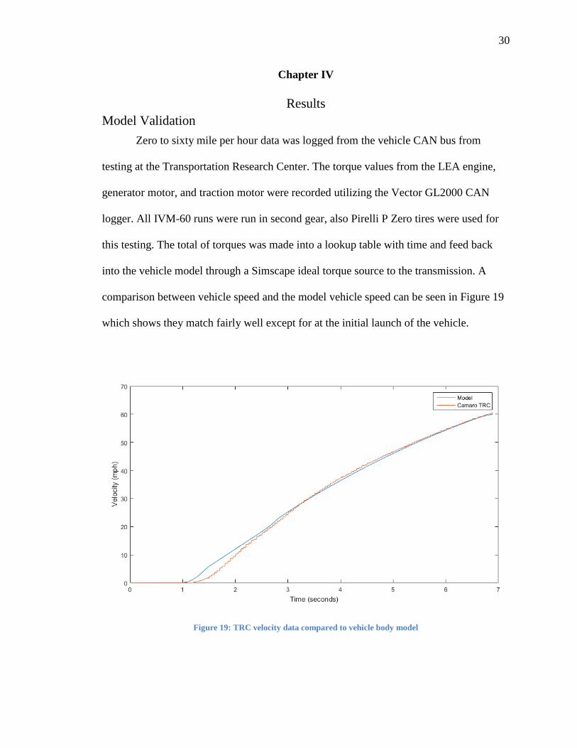
Model Validation

Zero to sixty mile per hour data was logged from the vehicle CAN bus from

testing at the Transportation Research Center. The torque values from the LEA engine,

generator motor, and traction motor were recorded utilizing the Vector GL2000 CAN

logger. All IVM-60 runs were run in second gear, also Pirelli P Zero tires were used for

this testing. The total of torques was made into a lookup table with time and feed back

into the vehicle model through a Simscape ideal torque source to the transmission. A

comparison between vehicle speed and the model vehicle speed can be seen in Figure 19

which shows they match fairly well except for at the initial launch of the vehicle.

Figure 19: TRC velocity data compared to vehicle body model

31

The wheel slip is compared in Figure 20 which has a discrepancy at the initial

launch but follows the same trend, this could be due to the delay of sending the wheel

speeds over CAN causing discretization compared to the model data shown where it is

continuous with no time delay. After the initial high wheel slip the slip percentage

matches with little difference.

Figure 20: TRC wheel slip compared to vehicle body model

IVM to sixty miles per hour is one of the benchmarks for measuring the

effectiveness of the traction control and launch control. These results are for the vehicle

driving on hi mu road surfaces, dry asphalt, shown in Table 1. The results shown here are

modeled with higher accessories loads of 1,000 watts, compared to the TRC testing

which was 670 watts. This was due to cold temperatures, 56 degrees Fahrenheit, during

this testing and the radiator fans being disabled. Decreasing the accessory loads on the

32

high voltage bus gives better electric machine performance by eliminating 330 watts to

offset. The engine was in its proper operating temperature range. Pirelli P Zero tires were

used for this testing. Automatic shifting starting in first going to second then third is what

was modeled in all cases. The TRC time was performed in second gear only due to

transmission issues. Due to this discrepancy, the percent decrease is calculated from the

model only.

Table 1: IVM to sixty times on dry asphalt

Run Time Percent

Decrease

Stock vehicle and TCS (TRC) (2nd gear only) 5.166 -

Model with no interventions 5.134 -

Model with powertrain torque reduction 4.941 3.76

Model with powertrain torque reduction and active brake

control

4.727 7.93

Model with powertrain torque reduction, active brake control

and launch control

4.675 8.94

33

Traction Control Dry Asphalt

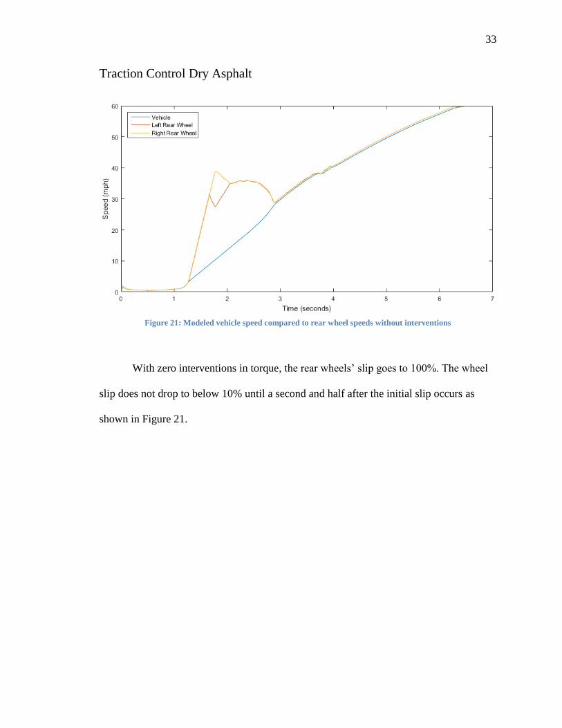
Figure 21: Modeled vehicle speed compared to rear wheel speeds without interventions

With zero interventions in torque, the rear wheels’ slip goes to 100%. The wheel

slip does not drop to below 10% until a second and half after the initial slip occurs as

shown in Figure 21.

34

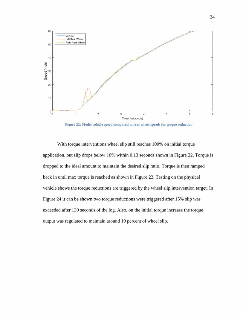
Figure 22: Model vehicle speed compared to rear wheel speeds for torque reduction

With torque interventions wheel slip still reaches 100% on initial torque

application, but slip drops below 10% within 0.13 seconds shown in Figure 22. Torque is

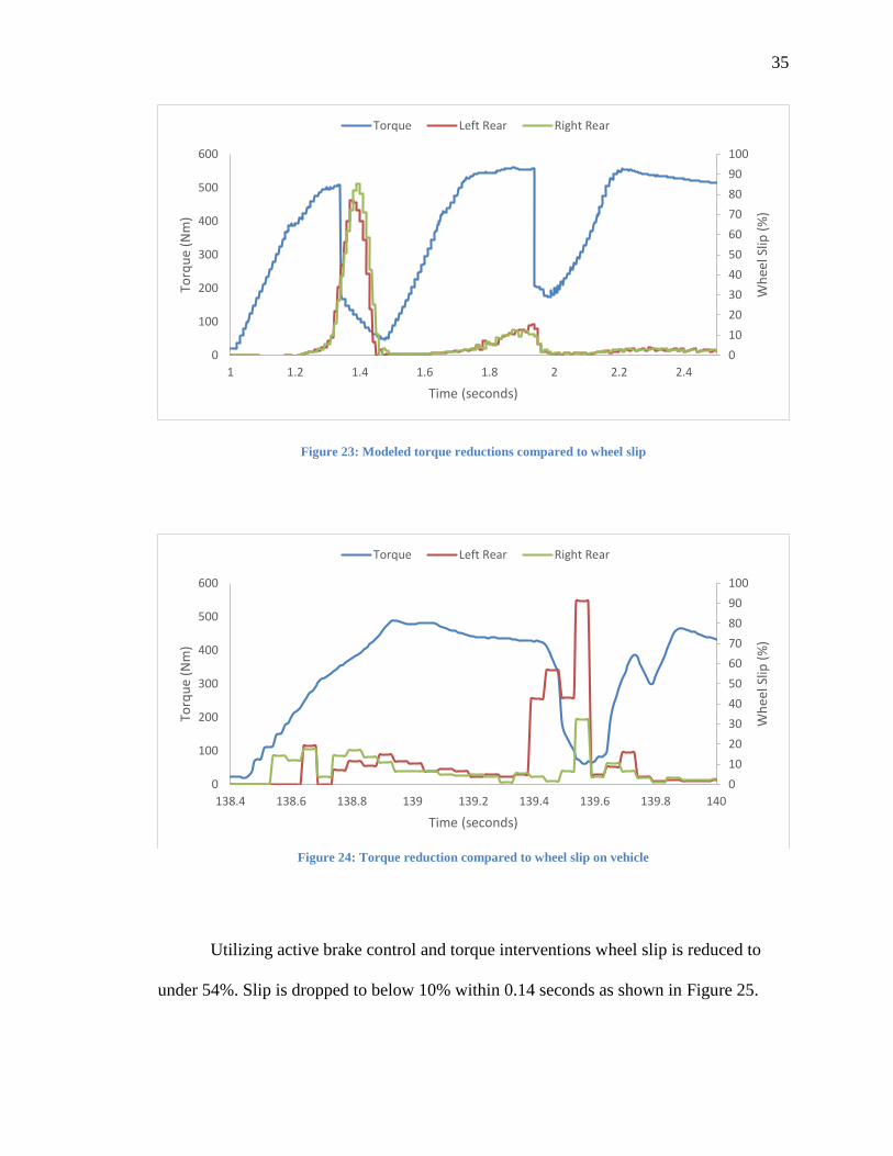
dropped to the ideal amount to maintain the desired slip ratio. Torque is then ramped

back in until max torque is reached as shown in Figure 23. Testing on the physical

vehicle shows the torque reductions are triggered by the wheel slip intervention target. In

Figure 24 it can be shown two torque reductions were triggered after 15% slip was

exceeded after 139 seconds of the log. Also, on the initial torque increase the torque

output was regulated to maintain around 10 percent of wheel slip.

35

Figure 23: Modeled torque reductions compared to wheel slip

Figure 24: Torque reduction compared to wheel slip on vehicle

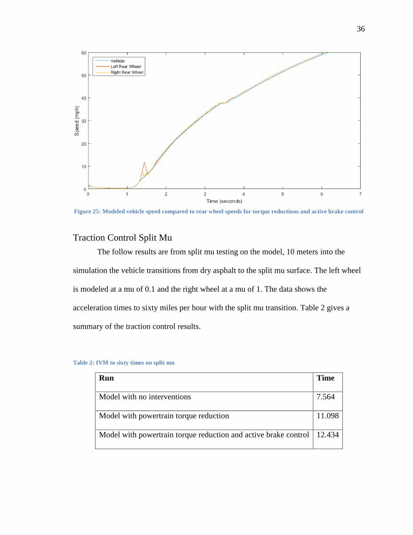
Utilizing active brake control and torque interventions wheel slip is reduced to

under 54%. Slip is dropped to below 10% within 0.14 seconds as shown in Figure 25.

0

10

20

30

40

50

60

70

80

90

100

0

100

200

300

400

500

600

1 1.2 1.4 1.6 1.8 2 2.2 2.4

Wh

eel S

lip (

%)

Torq

ue

(Nm

)

Time (seconds)

Torque Left Rear Right Rear

0

10

20

30

40

50

60

70

80

90

100

0

100

200

300

400

500

600

138.4 138.6 138.8 139 139.2 139.4 139.6 139.8 140

Wh

eel S

lip (

%)

Torq

ue

(Nm

)

Time (seconds)

Torque Left Rear Right Rear

36

Figure 25: Modeled vehicle speed compared to rear wheel speeds for torque reductions and active brake control

Traction Control Split Mu

The follow results are from split mu testing on the model, 10 meters into the

simulation the vehicle transitions from dry asphalt to the split mu surface. The left wheel

is modeled at a mu of 0.1 and the right wheel at a mu of 1. The data shows the

acceleration times to sixty miles per hour with the split mu transition. Table 2 gives a

summary of the traction control results.

Table 2: IVM to sixty times on split mu

Run Time

Model with no interventions 7.564

Model with powertrain torque reduction 11.098

Model with powertrain torque reduction and active brake control 12.434

37

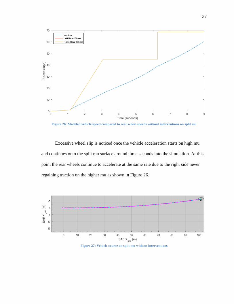
Figure 26: Modeled vehicle speed compared to rear wheel speeds without interventions on split mu

Excessive wheel slip is noticed once the vehicle acceleration starts on high mu

and continues onto the split mu surface around three seconds into the simulation. At this

point the rear wheels continue to accelerate at the same rate due to the right side never

regaining traction on the higher mu as shown in Figure 26.

Figure 27: Vehicle course on split mu without interventions

38

With the left tires on the low mu surface, the vehicle drifts to the left as it

accelerates up to sixty miles per hour as shown in Figure 27.

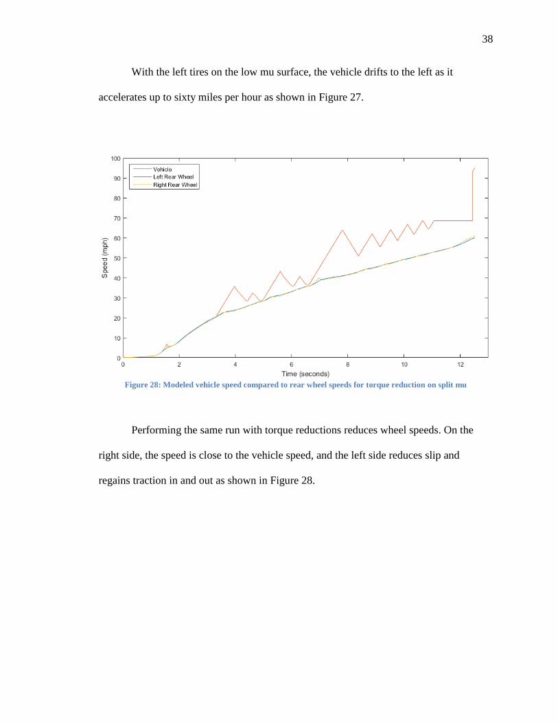
Figure 28: Modeled vehicle speed compared to rear wheel speeds for torque reduction on split mu

Performing the same run with torque reductions reduces wheel speeds. On the

right side, the speed is close to the vehicle speed, and the left side reduces slip and

regains traction in and out as shown in Figure 28.

39

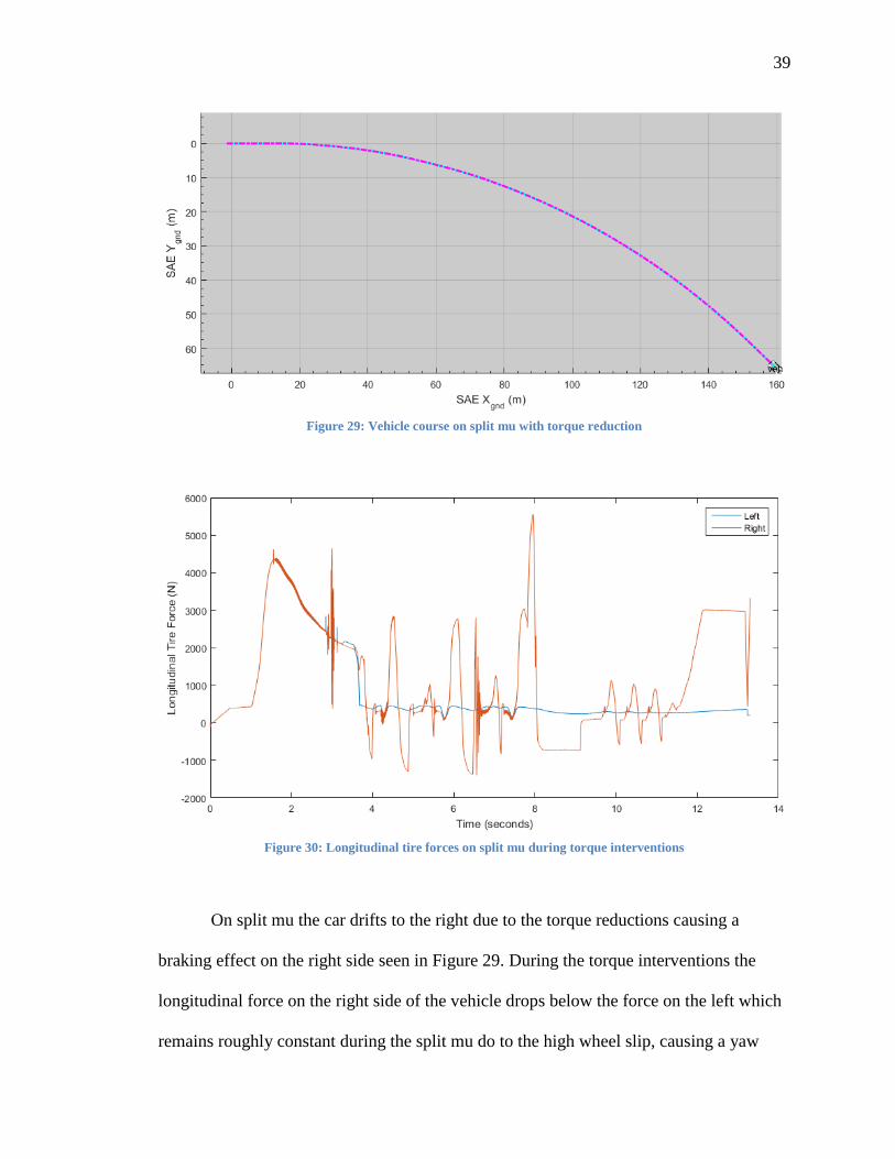
Figure 29: Vehicle course on split mu with torque reduction

Figure 30: Longitudinal tire forces on split mu during torque interventions

On split mu the car drifts to the right due to the torque reductions causing a

braking effect on the right side seen in Figure 29. During the torque interventions the

longitudinal force on the right side of the vehicle drops below the force on the left which

remains roughly constant during the split mu do to the high wheel slip, causing a yaw

40

moment on the vehicle. When an intervention is not taking place the longitudinal force on

the right will raise above the left side, this can be seen in Figure 30.

Figure 31: Modeled vehicle speed compared to rear wheel speeds for torque reduction and active brake control

on split mu

The final run with active braking and torque reductions on split mu yields a

straighter trajectory than the results of no interventions. The wheel speed of the slipping

driven wheel is reduced as shown in Figure 31. Stability is maintained, but acceleration is

decreased, reaching sixty by roughly 90 meters later as shown in Figure 32.

Figure 32: Vehicle course on split mu with torque reduction and active brake control

41

Launch Control

The benchmark for testing launch control is IVM to thirty miles per hour. The

results show improvements over normally accelerating the car from standstill. Figure 33

shows the modeled generator set RPM and traction motor RPM over time. Starting in the

staged RPM with the elevated speed on the generator set, followed by the clutch

engagement to full torque. A gain of 0.16 seconds was achieved, at 9 percent increase, by

utilizing launch control compared to normal acceleration from standstill with TCS.

Figure 33: Modeled launch control IVM-30 generator set vs traction motor RPM

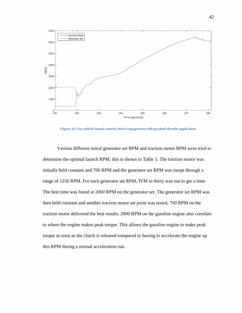
On the vehicle the clutch engagement was validated to the modeled simulation as

shown in Figure 34. The accelerator pedal was not fully depressed for this run resulting in

the slow increase in RPM after the clutch engaged.

42

Figure 34: On vehicle launch control clutch engagement with gradual throttle application

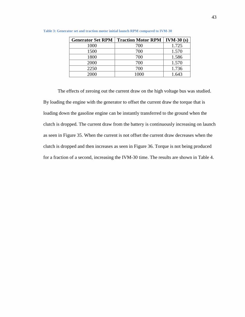
Various different initial generator set RPM and traction motor RPM were tried to

determine the optimal launch RPM, this is shown in Table 3. The traction motor was

initially held constant and 700 RPM and the generator set RPM was swept through a

range of 1250 RPM. For each generator set RPM, IVM to thirty was run to get a time.

The best time was found at 2000 RPM on the generator set. The generator set RPM was

then held constant and another traction motor set point was tested, 700 RPM on the

traction motor delivered the best results. 2000 RPM on the gasoline engine also correlate

to where the engine makes peak torque. This allows the gasoline engine to make peak

torque as soon as the clutch is released compared to having to accelerate the engine up

this RPM during a normal acceleration run.

43

Table 3: Generator set and traction motor initial launch RPM compared to IVM-30

Generator Set RPM Traction Motor RPM IVM-30 (s)

1000 700 1.725

1500 700 1.570

1800 700 1.586

2000 700 1.570

2250 700 1.736

2000 1000 1.643

The effects of zeroing out the current draw on the high voltage bus was studied.

By loading the engine with the generator to offset the current draw the torque that is

loading down the gasoline engine can be instantly transferred to the ground when the

clutch is dropped. The current draw from the battery is continuously increasing on launch

as seen in Figure 35. When the current is not offset the current draw decreases when the

clutch is dropped and then increases as seen in Figure 36. Torque is not being produced

for a fraction of a second, increasing the IVM-30 time. The results are shown in Table 4.

44

Figure 35: Model launch control with the engine offsetting the HV bus current draw

Figure 36: Modeled launch control without the engine offsetting the HV bus current draw

0

1000

2000

3000

4000

5000

6000

-500

-400

-300

-200

-100

0

4.5 5 5.5 6 6.5 7

RP

M

Cu

rren

t

Time (seconds)

Current Traction Motor Generator Set

0

1000

2000

3000

4000

5000

6000

-500

-400

-300

-200

-100

0

5 5.5 6 6.5 7 7.5

RP

M

Cu

rren

t

Time (seconds)

Current Traction Motor Generator Set

45

Table 4: Modeled launch control compared to no current offset

Run IVM-30 (s) Percent Decrease

TCS – torque interventions only 1.741 -

Launch control – 24 amp initial draw 1.603 7.93

Launch control – 0 amp initial draw 1.582 9.13

Launch control – 10 amp initial charge 1.618 7.06

A release of the clutch at 100 percent throttle is shown in Figure 37 resulting in a

quicker increase in RPM afterwards. Also, shown is the clutch disengagement and the

generator set targeting its set point and energy neutral high voltage bus. The torque of the

powertrain briefly goes negative on clutch engagement followed by a torque reduction by

TCS after full torque was reached shown in Figure 38.

Figure 37: On vehicle launch control clutch engagement with full throttle application

46

Figure 38: On vehicle launch control total torque with TCS torque reductions

47

Chapter V

Conclusions, and Future Work

Conclusions

Using a model based approach to developing a traction control and launch control

system in parallel to the hardware proved to be effective. Implementing a traction control

system that utilizes tire models in the controller allows the max torque that can be

transferred from the tires to the ground to be produced by the powertrain at every

controller cycle. If excessive wheel slip were to occur torque reductions are triggered that

target a desired slip ratio based on road surfaces, these interventions yield a 3.8 percent

decrease in time for IVM to sixty. Additionally, active braking is implemented on the

slipping wheels to achieve the desired slip ratio for the road surface, this yields a 7.9

percent increase in time for IVM to sixty.

On split mu situations the controller detects the change in wheel accelerations to

determine which side of the vehicle is on a lower friction coefficient surface. The base

torque reductions are implemented as well as the active braking on the slipping rear

wheel. Due to the lower friction coefficient the slip targets are lowered to get the optimal

acceleration for the surface. By doing so the vehicle is able to accelerate with very

minimal changes in its desired trajectory.

Launch control was used to elevate the generator set RPM to get into a region of

higher torque. The current draw was offset by the engine producing torque and the

generator IMG generating current. By producing an energy neutral high voltage bus this

allows the full discharge buffer to be utilized; normally it would be decreasing by having

the traction motor spinning at idle to keep the automatic transmission clutches engaged.

Once the launch criteria are met the clutch is engaged between the generator set and

48

traction motor and all torque is delivered to the rear wheels. This yielded a 10 percent

decrease in time from IVM to thirty.

The modeled results were shown to correlate to the on vehicle test results, but a

full comparison could not be conducted due to vehicle transmission issues.

Future Work

If time were permitted a couple of topics for future refinement would be

recommended. First, in split mu scenarios torque increases would be implemented by the

amount of brake torque applied to the slipping wheel to counter the yaw moment of the

vehicle, reducing the amount of counter steering necessary by the driver. This would help

keep the vehicle in a straight line trajectory. Second would be to perform a more

extensive parameter optimization for the ideal launch RPM points for the generator set

and traction motor. This would further enhance the IVM to sixty times for the vehicle.

49

Appendix A

Bibliography Beal, C. E. (2016). Independent Wheel Effects in Real Time Estimation of Tire-Road

Friction Coefficient from Steering Torque. IFAC-PapersOnLine, 319-326.

Cerdeira-Corujo, M., Costas, A., Delgado, E., & Barreiro, A. (2016). Comparative

analysis of gain-scheduled wheel slip reset controllers with different reset

strategies in automotive brake systems. Lecture Notes in Electrical Engineering,

751-761.

Delarammatikas, F. T. (2011). The traction control system of the 2011 cooper union

FSAE vehicle. SAE Technical Papers.

Evangelou, S. A., & Shabbir, W. (2016). Control Engineering Practice. IFAC-

PapersOnLine, 533-540.

Fingas, J. (2016, 10 08). Germany call for a ban on combustion engine cars by 2030.

Retrieved from Engadget: https://www.engadget.com

Giani, P., Tanelli, M., Savaresi, S. M., & Santucci, M. (2013). Launch control for sport

motorcycles: A clutch-based approach. Control Engineering Practice, 1756-1766.

Gillespie, T. D. (1992). Fundamentals of Vehicle Dynamics. Warrendale: Society of

Automotive Engineers, Inc.

Kadijk, G., & Ligterink, N. (2012). Road load determination of passenger cars.

Plesmanweg: Ministry of Infrastructure and the Environment.

Kuntanapreeda, S. (2014). Traction Control of Electric Vehicles Using Sliding-Mode

Controller with Tractive Force Observer. International Journal of Vehicular

Technology, 9.

Kuntanapreeda, S. (2015). Super-twisting sliding-mode traction control of vehicles with

tractive force observer. Control Engineering Practice, 26-36.

Li, G., Wang, T., Zhang, R., Gu, F., & Shen, J. (2015). An Improved Optimal Slip Ratio

Prediction considering Tyre Inflation Pressure Changes. Journal of Control

Science and Engineering, 8.

Li, H.-Z., Li, L., He, L., Kang, M.-X., Song, J., Yu, L.-Y., & Wu, C. (2012). PID Plus

Fuzzy Logic for Torque Control in Traction Control System. International

Journal of Automotive Technology, 441-450.

Liu, G., & Jin, L. (2016). A Study of Coordinated Vehicle Traction Control System

Based on Optimal Slip Ratio Algorithm. Mathematical Problems in Engineering,

10.

Liu, Y. H., Li, T., Yang, Y. Y., Ji, X. W., & Wu, J. (2017). Estimation of tire-road

friction coefficient based on combined APF-IEKF and iteration algorithm.

Mechanical Systems and Signal Processing, 25-35.

Lyon, K., Philipp, M., & Grommes, E. (1994). Traction control for a formula 1 race car:

Conceptual design, algorithm development, and calibration methodology. SAE

Technical Papers.

Milliken, W. F., & Milliken, D. L. (1995). Race Car Vehicle Dynamics. Warrendale:

Society of Automotive Engineers, Inc.

NewsRx. (2015). Toyota Motor Engineering & Manufacturing North America, Inc.;

Patent Issued for Hybrid Vehicle Launch Control. Journal of Engineering.

50

Pacejka, H. B., & Besselink, I. (2012). Tire and Vehicle Dynamics. Waltham: Elsevier

Ltd.

Rajamani, R., Phanomchoeng, G., Piyabongkarn, D., & Lew, J. Y. (2012). Algorithms for

Real-Time Estimation of Individual Wheel Tire-Road Friction Coefficients.

IEEE/ASME Transactions on Mechatronics, 1183-1195.

Robert Bosch GmbH. (2004). Automotive Handbook. Karlsruhe: Robert Bosch GmbH.

Sharifzadeh, M., Akbari, A., Timpone, F., & Daryani, R. (2016). Vehicle tyre/road

interaction modeling and identification of its parameters using real-time trust-

region methods. IFAC-PapersOnLine, 111-116.

Shi, J., Li, X., Lu, T., & Zhang, J. (2012). Development of a New Traction Control

System for Vehicles with Automatic Transmissions. International Journal of

Automotive Technology, 743-750.

Tanelli, M., Vecchio, C., Corno, M., Ferrara, A., & Savaresi, S. M. (2009). Traction

control for ride-by-wire sport motorcycles: A second-order sliding mode

approach. IEEE Transactions on Industrial Electronics, 3347-3356.

Urda, P., Cabrera, J. A., Castillo, J. J., & Guerra, A. J. (2015). An intelligent traction

control for motorcycles. The Dynamics of Vehicles on Roads and Tracks, 809-

822.

Villagra, J. (2010). A diagnosis-based approach for tire-road forces and maximum

friction estimation. Control Engineering Practice, 174-184.