Tractable Classes of Metric Temporal Problems with Domain Rules

T. K. Satish KumarComputer Science Division

University of California, Berkeleytksk@eecs.berkeley.edu

Abstract

In this paper, we will deal with some important kinds of met-ric temporal reasoning problems that arise in many real-lifesituations. In particular, events X0, X1 . . . XN are modeledas time points, and a constraint between the execution timesof two events Xi and Xj is either simple temporal (of theform Xi − Xj ∈ [a, b]), or has a connected feasible regionthat can be expressed using a finite set of domain rules each inturn of the form Xi ∈ [a, b] → Xj ∈ [c, d] (and converselyXj ∈ [e, f ] → Xi ∈ [g, h]). We argue that such rules areuseful in capturing important kinds of non-monotonic rela-tionships between the execution times of events when theyare governed by potentially complex (external) factors. Ourpolynomial-time (deterministic and randomized) algorithmsfor solving such problems therefore enable us to efficientlydeal with very expressive representations of time.

IntroductionEfficient algorithms for solving problems involving rich rep-resentations of time are crucial to many applications in AI.Several tasks in planning and scheduling, for example, in-volve reasoning about temporal constraints between actionsand propositions in partial plans (Smith et al 2000). Thesetasks may include threat resolution in partial order plan-ning, analyzing resource consumption envelopes to guidethe search for a good plan (see (Muscettola 2002) and (Ku-mar 2003)), etc. Among the important formalisms used forreasoning with metric time are simple temporal problems(STPs) and disjunctive temporal problems (DTPs).

Unlike DTPs, STPs can be solved in polynomial time, butare not as expressive as DTPs. An STP is characterized by agraph G = 〈X , E〉, where X = {X0, X1 . . . XN} is a set ofevents (X0 is the “beginning of the world” node and is setto 0 by convention), and e = 〈Xi, Xj〉 ∈ E , annotated withthe bounds [LB(e), UB(e)], is a simple temporal constraintbetween Xi and Xj indicating that Xj must be scheduledbetween LB(e) and UB(e) seconds after Xi is scheduled(LB(e) ≤ UB(e)).

DTPs are significantly more expressive than STPs, andallow for disjunctive constraints. The general form of aDTP is as follows. We are given a set of events X ={X0, X1 . . . XN} (X0 is the “beginning of the world” node

Copyright c© 2006, American Association for Artificial Intelli-gence (www.aaai.org). All rights reserved.

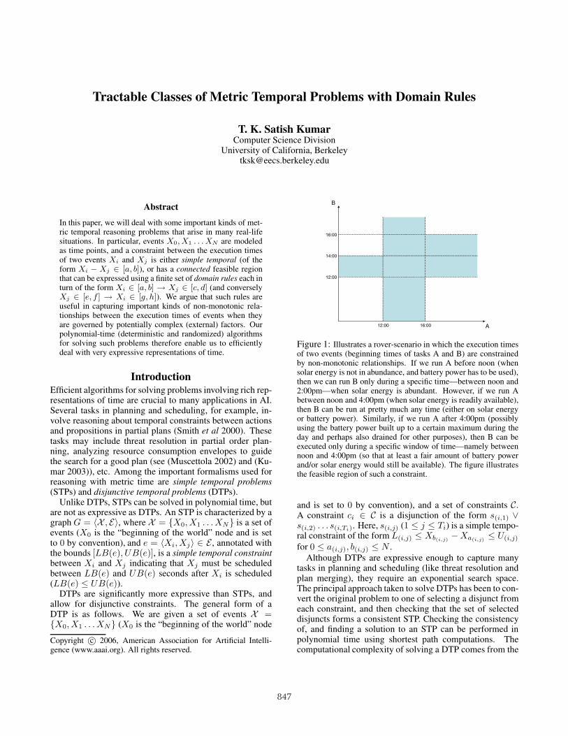
Figure 1: Illustrates a rover-scenario in which the execution timesof two events (beginning times of tasks A and B) are constrainedby non-monotonic relationships. If we run A before noon (whensolar energy is not in abundance, and battery power has to be used),then we can run B only during a specific time—between noon and2:00pm—when solar energy is abundant. However, if we run Abetween noon and 4:00pm (when solar energy is readily available),then B can be run at pretty much any time (either on solar energyor battery power). Similarly, if we run A after 4:00pm (possiblyusing the battery power built up to a certain maximum during theday and perhaps also drained for other purposes), then B can beexecuted only during a specific window of time—namely betweennoon and 4:00pm (so that at least a fair amount of battery powerand/or solar energy would still be available). The figure illustratesthe feasible region of such a constraint.

and is set to 0 by convention), and a set of constraints C.A constraint ci ∈ C is a disjunction of the form s(i,1) ∨s(i,2) . . . s(i,Ti). Here, s(i,j) (1 ≤ j ≤ Ti) is a simple tempo-ral constraint of the form L(i,j) ≤ Xb(i,j) −Xa(i,j) ≤ U(i,j)

for 0 ≤ a(i,j), b(i,j) ≤ N .Although DTPs are expressive enough to capture many

tasks in planning and scheduling (like threat resolution andplan merging), they require an exponential search space.The principal approach taken to solve DTPs has been to con-vert the original problem to one of selecting a disjunct fromeach constraint, and then checking that the set of selecteddisjuncts forms a consistent STP. Checking the consistencyof, and finding a solution to an STP can be performed inpolynomial time using shortest path computations. Thecomputational complexity of solving a DTP comes from the

847

Figure 2: Presents an elaborate real-life example about an agenthaving to plan her day’s schedules. Suppose X0 corresponds to12:00am. The agent chooses to sleep between 6 and 8 hours, andhave breakfast for anytime between 1 and 2 hours. After this, shehas to go to the shopping store; shop there for anytime between 2and 3 hours; and come back home before 4:00pm. The constraint(between X2 and X3) describing her travel options between homeand the shopping store is best described by the set of domain rulesas in the accompanying diagram. If the agent starts out between6:00am and 6:30am, then she can accompany a friend going tothe same destination in his/her car and reach her destination any-time between 8:00am and 8:30am. However, between 6:30am and7:30am, the only option she has is to take the city bus. If she takesthe bus between 6:30am and 7:00am, she can reach her destinationanytime between 7:30am and 9:30am—with the large uncertaintycoming from the (un)availability of an express bus and/or exter-nal traffic-related factors. Similarly, if she takes the bus between7:00am and 7:30am, she can get to her destination anytime be-tween 8:00am and 10:00am. Finally, if she is willing to wait until7:30am and possibly spend more money, she can take an expresstrain to reach her destination anytime between 9:00am and 9:30am.Her travel options between the shopping store and back home (con-straint between X4 and X5) can be similarly argued.

fact that there are an exponentially large number of disjunctcombinations possible. This “disjunct selection problem”can also be cast as a constraint satisfaction problem (CSP),or a satisfiability problem (SAT) and solved using standardsearch techniques applicable for them (see (Tsamardinosand Pollack 2003) and (Armando et al 2004)).

In (Kumar 2005a), a tractable class of DTPs called re-stricted DTPs (RDTPs) is identified. In RDTPs, any ci ∈ Cis restricted to be of one of the following types: (Type 1)(L ≤ Xb − Xa ≤ U), (Type 2) (L1 ≤ Xa ≤ U1) ∨ (L2 ≤Xa ≤ U2) . . . (LTi ≤ Xa ≤ UTi), or (Type 3) (L1 ≤ Xa ≤U1)∨(L2 ≤ Xb ≤ U2). RDTPs are amenable to very simplepolynomial-time algorithms (Kumar 2005a).

In this paper, however, instead of dealing with disjunc-tions explicitly, we will deal with important kinds of met-ric temporal reasoning problems where the direct constraintbetween the execution times of two events Xi and Xj isitself more naturally expressive. In particular, the eventsX0, X1 . . .XN are modeled as time points, and a constraintbetween the execution times of two events Xi and Xj is ei-ther simple temporal or has a connected feasible region thatcan be expressed using a finite set of domain rules each inturn of the form Xi ∈ [a, b] → Xj ∈ [c, d] (and converselyXj ∈ [e, f ] → Xi ∈ [g, h]). We argue that such rules areuseful in capturing important kinds of non-monotonic rela-

Figure 3: Illustrates the notion of a smooth constraint (left side).The right side illustrates the fact that a simple temporal constraintis smooth. At any infeasible point (A) there exist two directionssuch that moving along at least one of them (by a tiny amount)decreases the L1-distance to the solution (A∗), no matter where itis placed in the feasible region of the constraint.

tionships between the execution times of events when theyare governed by potentially complex (external) factors. Ourpolynomial-time (deterministic and randomized) algorithmsfor solving such problems therefore enable us to efficientlydeal with very expressive representations of time.

We note that although a rule of the form Xi ∈ [a, b] →Xj ∈ [c, d] is equivalent to the disjunction (Xi < a)∨(Xi >b)∨(Xj ∈ [c, d]), it is not of a type allowed by RDTPs. Fur-ther, treating the disjunctions explicitly will result in a DTPwhich requires an exponential search space. The key ideain this paper is to show that although each rule consideredindividually is equivalent to a disjunction of the above men-tioned kind, when all the rules are treated together, they canbe made amenable to very simple polynomial-time (deter-ministic and randomized) algorithms.

Figure 1 shows an example of the kinds of constraints ex-pressible by domain rules (that are going to be dealt within this paper). In particular, it illustrates a rover scenario inwhich the execution times of two events (beginning timesof two tasks A and B respectively) are constrained by non-monotonic relationships. (Note that the problem is allowedto contain other such constraints or even other simple tem-poral constraints.) Non-monotonic relationships betweenthe execution times of events occur fairly naturally in manyproblem domains, and are mostly a result of the effects ofcomplex (external) factors like the presence of reservoirs ofresources (e.g. battery power and sunlight), presence of mul-tiple options (see next example), etc. Such non-monotonicrelationships can very often be appropriately expressed us-ing a finite set of domain rules, but cannot be captured bysimple temporal constraints alone. Figure 2 presents a moreelaborate real-life example.

Smoothness and Temporal ProblemsIn (Kumar 2005b), a theory of random walks is shown to beuseful in identifying tractable classes of constraints referredto as smooth constraints. A binary constraint between Xi

and Xj (under an ordering of their domain values) is said to

848

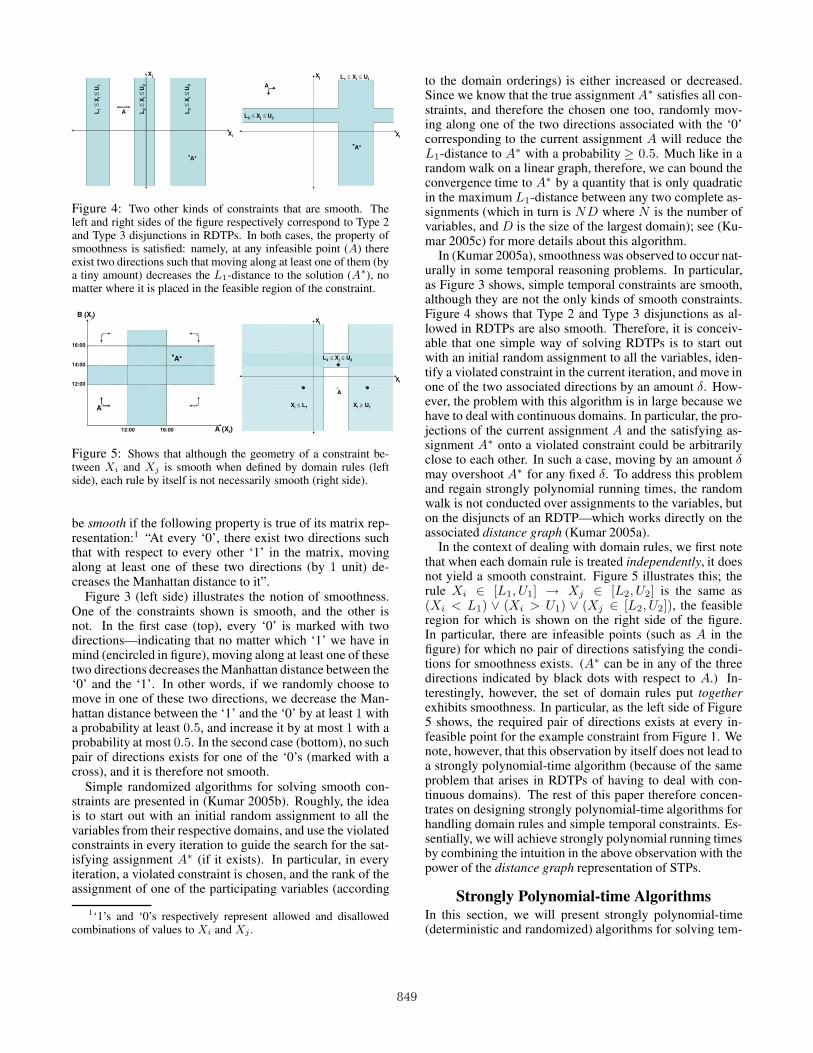
Figure 4: Two other kinds of constraints that are smooth. Theleft and right sides of the figure respectively correspond to Type 2and Type 3 disjunctions in RDTPs. In both cases, the property ofsmoothness is satisfied: namely, at any infeasible point (A) thereexist two directions such that moving along at least one of them (bya tiny amount) decreases the L1-distance to the solution (A∗), nomatter where it is placed in the feasible region of the constraint.

Figure 5: Shows that although the geometry of a constraint be-tween Xi and Xj is smooth when defined by domain rules (leftside), each rule by itself is not necessarily smooth (right side).

be smooth if the following property is true of its matrix rep-resentation:1 “At every ‘0’, there exist two directions suchthat with respect to every other ‘1’ in the matrix, movingalong at least one of these two directions (by 1 unit) de-creases the Manhattan distance to it”.

Figure 3 (left side) illustrates the notion of smoothness.One of the constraints shown is smooth, and the other isnot. In the first case (top), every ‘0’ is marked with twodirections—indicating that no matter which ‘1’ we have inmind (encircled in figure), moving along at least one of thesetwo directions decreases the Manhattan distance between the‘0’ and the ‘1’. In other words, if we randomly choose tomove in one of these two directions, we decrease the Man-hattan distance between the ‘1’ and the ‘0’ by at least 1 witha probability at least 0.5, and increase it by at most 1 with aprobability at most 0.5. In the second case (bottom), no suchpair of directions exists for one of the ‘0’s (marked with across), and it is therefore not smooth.

Simple randomized algorithms for solving smooth con-straints are presented in (Kumar 2005b). Roughly, the ideais to start out with an initial random assignment to all thevariables from their respective domains, and use the violatedconstraints in every iteration to guide the search for the sat-isfying assignment A∗ (if it exists). In particular, in everyiteration, a violated constraint is chosen, and the rank of theassignment of one of the participating variables (according

1‘1’s and ‘0’s respectively represent allowed and disallowedcombinations of values to Xi and Xj .

to the domain orderings) is either increased or decreased.Since we know that the true assignment A∗ satisfies all con-straints, and therefore the chosen one too, randomly mov-ing along one of the two directions associated with the ‘0’corresponding to the current assignment A will reduce theL1-distance to A∗ with a probability ≥ 0.5. Much like in arandom walk on a linear graph, therefore, we can bound theconvergence time to A∗ by a quantity that is only quadraticin the maximum L1-distance between any two complete as-signments (which in turn is ND where N is the number ofvariables, and D is the size of the largest domain); see (Ku-mar 2005c) for more details about this algorithm.

In (Kumar 2005a), smoothness was observed to occur nat-urally in some temporal reasoning problems. In particular,as Figure 3 shows, simple temporal constraints are smooth,although they are not the only kinds of smooth constraints.Figure 4 shows that Type 2 and Type 3 disjunctions as al-lowed in RDTPs are also smooth. Therefore, it is conceiv-able that one simple way of solving RDTPs is to start outwith an initial random assignment to all the variables, iden-tify a violated constraint in the current iteration, and move inone of the two associated directions by an amount δ. How-ever, the problem with this algorithm is in large because wehave to deal with continuous domains. In particular, the pro-jections of the current assignment A and the satisfying as-signment A∗ onto a violated constraint could be arbitrarilyclose to each other. In such a case, moving by an amount δmay overshoot A∗ for any fixed δ. To address this problemand regain strongly polynomial running times, the randomwalk is not conducted over assignments to the variables, buton the disjuncts of an RDTP—which works directly on theassociated distance graph (Kumar 2005a).

In the context of dealing with domain rules, we first notethat when each domain rule is treated independently, it doesnot yield a smooth constraint. Figure 5 illustrates this; therule Xi ∈ [L1, U1] → Xj ∈ [L2, U2] is the same as(Xi < L1) ∨ (Xi > U1) ∨ (Xj ∈ [L2, U2]), the feasibleregion for which is shown on the right side of the figure.In particular, there are infeasible points (such as A in thefigure) for which no pair of directions satisfying the condi-tions for smoothness exists. (A∗ can be in any of the threedirections indicated by black dots with respect to A.) In-terestingly, however, the set of domain rules put togetherexhibits smoothness. In particular, as the left side of Figure5 shows, the required pair of directions exists at every in-feasible point for the example constraint from Figure 1. Wenote, however, that this observation by itself does not lead toa strongly polynomial-time algorithm (because of the sameproblem that arises in RDTPs of having to deal with con-tinuous domains). The rest of this paper therefore concen-trates on designing strongly polynomial-time algorithms forhandling domain rules and simple temporal constraints. Es-sentially, we will achieve strongly polynomial running timesby combining the intuition in the above observation with thepower of the distance graph representation of STPs.

Strongly Polynomial-time AlgorithmsIn this section, we will present strongly polynomial-time(deterministic and randomized) algorithms for solving tem-

849

Figure 6: Illustrates constraints that can be expressed using do-main rules. The (connected) feasible region on the top left side ofthe figure can be expressed using domain rules with either Xi orXj as the tail variable. The (connected) feasible region on the topright side of the figure, however, can be expressed using domainrules only with Xi as the tail variable (and not with Xj). In the lastcase (bottom), the feasible region can be expressed using domainrules with either Xi or Xj as the tail variable, but is not connected.Only the first case qualifies as a smooth constraint.

poral problems with domain rules. The correctness of the al-gorithms is proved in the Lemmas that follow. For notationalconvenience, we will refer to the constraint (L ≤ Xa ≤ U )as Xa ∈ [L, U ]. For any interval I = [L, U ], we will de-note its left end-point (viz. L) by L(I), and its right end-point (viz. U ) by R(I). We will also say that an intervalI1 = [L1, U1] subsumes another interval I2 = [L2, U2] (de-noted I2 ⊆ I1) if and only if L1 ≤ L2 and U2 ≤ U1.

We note once again that we are dealing with temporal con-straints that are either simple temporal (between Xi and Xj),or have a connected feasible region that can be expressedby a finite set of domain rules, each in turn of the form:Xi ∈ Ii1 → Xj ∈ Ij1 (and conversely Xj ∈ Ij2 → Xi ∈Ii2). It is important that the constraint be expressible in bothways and have a connected feasible region in order for it tobe smooth (as illustrated in Figure 6). This is because bi-nary smooth constraints have been shown to be equivalentto connected row-convex (CRC) constraints (see (Deville etal 1999) and (Kumar 2005c)). The top left side of the figurehas a connected feasible region which can be expressed asthree rules of the form Xi ∈ Ip → Xj ∈ Iq (namely Xi ∈[0, a1] → Xj ∈ [b1, b3], Xi ∈ [a1, a2] → Xj ∈ [0,∞] andXi ∈ [a2,∞] → Xj ∈ [b2, b4]). Here, Xi is referred to asthe tail variable, and Xj as the head variable. Moreover, theconstraint can also be expressed using five rules of the formXj ∈ Iq → Xi ∈ Ip i.e. with Xj as the tail variable (namelyXj ∈ [0, b1] → Xi ∈ [a1, a2], Xj ∈ [b1, b2] → Xi ∈[0, a2], Xj ∈ [b2, b3] → Xi ∈ [0,∞], Xj ∈ [b3, b4] →Xi ∈ [a1,∞] and Xj ∈ [b4,∞] → Xi ∈ [a1, a2]). Thus,it satisfies the properties required for smoothness. The top

Figure 7: Three basic cases in which a constraint between Xi

and Xj (with a connected feasible region) can be expressed usingdomain rules with either Xi or Xj as the tail variable. Cases (1)and (2) (top two cases) have a monotonic behavior in terms of thelower and upper end-points of the intervals Ij1, Ij2 . . . Ijk (usingXi as the tail). In case (3) (bottom case), this is not true. However,the subsumption relationships between the intervals Ij1, Ij2 . . . Ijk

follow a bitonic sequence—i.e. Ij1 ⊆ Ij2 ⊆ Ij3 ⊇ Ij4.

right side of the figure, however, cannot be expressed in thisfashion, and is therefore not smooth. Although it can be ex-pressed as three rules of the form Xi ∈ Ip → Xj ∈ Iq

(namely Xi ∈ [0, a1] → Xj ∈ [b1, b4], Xi ∈ [a1, a2] →Xj ∈ [b3, b6] and Xi ∈ [a2,∞] → Xj ∈ [b2, b5]), it cannotbe expressed using rules of the form Xj ∈ Iq → Xi ∈ Ip.In particular, this is because when Xj ∈ [b2, b3], Xi is in[0, a1] ∪ [a2,∞] and not within a continuous interval. Thebottom case in the figure shows that although the constraintcan be expressed as a finite set of domain rules using eitherXi or Xj as the tail variable, it is still not a smooth constraintbecause the feasible region is not connected.2 Put together,not all non-monotonic relationships are smooth; but thoseconstraints that have a connected feasible region and thatcan be expressed as domain rules using any of the two vari-ables as the tail variable are certainly smooth. As we willsee later in this section, these cases can be made amenableto simple polynomial-time (deterministic and randomized)algorithms. We also note that the examples presented in theIntroduction satisfy our requirements for smoothness.

Consider a constraint between Xi and Xj (with a con-nected feasible region) that can be expressed as a finite setof domain rules using either of the variables as the tail vari-able. Without loss of generality, let us assume that we use

2Strictly speaking, smoothness does not a priori prohibit dis-connected feasible regions (e.g. Type 2 disjunctions of RDTPs)provided they become connected after removing entire horizon-tal and vertical strips of infeasible regions (analogous to rows andcolumns with only ‘0’s in the discrete case). Although these casescan also be taken care of in the various Lemmas, we will not dealwith them explicitly in the rest of this paper (to retain simplicity).

850

ALGORITHM: SOLVE-STP-DOMAIN-RULESINPUT: Events {X0, X1 . . . XN}, with a constraint be-tween Xi and Xj being either simple temporal or havinga connected feasible region expressible as a finite set ofdomain rules using either Xi or Xj as the tail variable.OUTPUT: A solution s (if it exists).(1) Cast the problem as a “disjunct selection problem”using meta-variables W = {W1, W2 . . . WR} such that:

(a) A variable W ∈ W corresponds to a constraint ofthe form Xi ∈ Ii1 → Xj ∈ Ij1, Xi ∈ Ii2 → Xj ∈ Ij2

. . . Xi ∈ Iik → Xj ∈ Ijk (domain rules).(b) The domain of W is = {(Xi ∈ Ii1 ∧ Xj ∈ Ij1),(Xi ∈ Ii2 ∧ Xj ∈ Ij2) . . . (Xi ∈ Iik ∧ Xj ∈ Ijk)}(c) The ordering on the domain values of W is thenominal ordering—i.e. ascending order of the intervalsdefined for the tail variable.

(2) For every Wi and Wj in W , build a binary constraintas follows:

(a) An instantiation of disjuncts to Wi and Wj isdisallowed, if and only if, together with the rest of thesimple temporal constraints, they introduce a negativecycle in the underlying distance graph.

(3) Solve these binary constraints using the (deterministicor randomized) procedures for solving CRC constraints.(4) RETURN: s = SOLVE-STP (induced STP).END ALGORITHM

Figure 8: Strongly polynomial-time (deterministic and random-ized) algorithms for solving simple temporal constraints with do-main rules (of the special kinds identified in the paper). We notethat a “disjunct” involves constraining intervals for two variables.

Xi as the tail variable. Then, a natural ordering exists on therules Xi ∈ Ii1 → Xj ∈ Ij1, Xi ∈ Ii2 → Xj ∈ Ij2 . . . Xi ∈Iik → Xj ∈ Ijk—namely, the increasing order of the in-tervals Ii1, Ii2 . . . Iik .3 We will refer to this ordering as thenominal ordering of the domain rules with respect to Xi.For example, the rules Xi ∈ [0, 2] → Xj ∈ [3, 5], Xi ∈[10,∞] → Xj ∈ [7, 14] and Xi ∈ [2, 10] → Xj ∈ [1,∞]are arranged as Xi ∈ [0, 2] → Xj ∈ [3, 5], Xi ∈ [2, 10] →Xj ∈ [1,∞] and Xi ∈ [10,∞] → Xj ∈ [7, 14] in the nomi-nal ordering with respect to the tail variable Xi.

Figure 7 shows the three basic cases in which a constraintbetween Xi and Xj (with a connected feasible region) canbe expressed using domain rules with either Xi or Xj asthe tail variable. (Other cases are possible by certain com-binations of these basic cases, and their tractability can beestablished using arguments similar to the ones presentedin this paper; but in the interest of simplicity, we will notdeal with them explicitly.) Cases (1) and (2) have a mono-tonic behavior in terms of the lower and upper end-points ofthe intervals Ij1, Ij2 . . . Ijk (using Xi as the tail variable).The more interesting case is (3) where the subsumptionrelationships between the intervals Ij1, Ij2 . . . Ijk follow abitonic sequence—i.e. Ij1 ⊆ Ij2 . . . Ij(q∗−1) ⊆ Ijq∗ ⊇

3We will assume that Ii1, Ii2 . . . Iik are non-overlapping; oth-erwise, we can rewrite the rules in such a canonical form.

Ij(q∗+1) . . . Ij(k−1) ⊇ Ijk (for some 1 ≤ q∗ ≤ k). We willdeal only with the more interesting case in (3). The casesin (1) and (2) are simple generalizations of the Lemmas pre-sented in (Kumar 2005a). Case (3), however, requires dif-ferent arguments (presented in the Lemmas below). We usethe result that a consistent schedule exists for an STP if andonly if its associated distance graph does not contain anynegative cycles (Dechter et al 1991).

For any finite set of domain rules Xi ∈ Ii1 → Xj ∈ Ij1,Xi ∈ Ii2 → Xj ∈ Ij2 . . . Xi ∈ Iik → Xj ∈ Ijk , sincethe intervals Ii1, Ii2 . . . Iik are non-overlapping, all of theimplications (rules) would be satisfied if we ensure that both(Xi ∈ Iih) and (Xj ∈ Ijh) are true for some 1 ≤ h ≤ k.Because of this, we can view our problem as a meta-levelCSP where the meta-level variables are associated withevery set of rules of the form Xi ∈ Ii1 → Xj ∈ Ij1, Xi ∈Ii2 → Xj ∈ Ij2 . . . Xi ∈ Iik → Xj ∈ Ijk , and theirdomains are respectively {(Xi ∈ Ii1 ∧ Xj ∈ Ij1), (Xi ∈Ii2 ∧ Xj ∈ Ij2) . . . (Xi ∈ Iik ∧ Xj ∈ Ijk)}. The goal isthen to instantiate these meta-level variables in such a waythat the resulting simple temporal constraints (in additionto the other simple temporal constraints already specifiedin the problem) do not induce a negative cost cycle in theunderlying distance graph.

Lemma 1: The choice (Xi ∈ Ip ∧Xj ∈ Iq) is equivalent toadding the edges 〈X0, Xi〉 annotated with R(Ip), 〈Xi, X0〉annotated with −L(Ip), 〈X0, Xj〉 annotated with R(Iq)and 〈Xj , X0〉 annotated with −L(Iq) to the distance graphwithout creating a negative cycle.Proof: If we have to ensure that the variable Xi is in theinterval Ip, we have to make sure that Xi−X0 ≤ R(Ip) andXi − X0 ≥ L(Ip). Retaining the semantics of the distancegraph where the constraint Xb − Xa ≤ w is specified bythe edge 〈Xa, Xb〉 annotated with w, this corresponds tothe addition of the edges 〈X0, Xi〉 annotated with R(Ip),and 〈Xi, X0〉 annotated with −L(Ip), to the distance graphwithout creating an inconsistency (which is characterizedby the presence of a negative cycle). Similarly, the othertwo edges are required for ensuring that Xj ∈ Iq .

We define a conflict to be an instantiation of a set ofmeta-level variables that results in an inconsistency with therest of the simple temporal constraints. We define a minimalconflict to be a conflict no proper subset of which is alsoa conflict. It is easy to see that an instantiation of a set ofmeta-level variables is consistent (with the rest of the simpletemporal constraints in the problem) if and only if there isno subset of this set that constitutes a minimal conflict.

Lemma 2: The size of a minimal conflict is ≤ 2.Proof: Suppose we try to instantiate a set of meta-levelvariables W1, W2 . . .Wh. Since instantiating any meta-levelvariable W requires committing to some variables XiW

and XjW to respectively be within some intervals IpW

and IqW , we would have to add the following edges tothe distance graph: 〈X0, XiW 〉 annotated with R(IpW ),〈XiW , X0〉 annotated with −L(IpW ), 〈X0, XjW 〉 annotatedwith R(IqW ), and 〈XjW , X0〉 annotated with −L(IqW )

851

(for all W ∈ {W1, W2 . . . Wh}). We will refer to theseedges as “special” edges. Knowing that the distance graphinitially does not contain any negative cycles (because anyinconsistency in the given simple temporal constraints canbe caught right away), if a negative cycle is newly created, itmust involve one of the “special” edges. Since all “special”edges have X0 as an end point, the negative cycle mustcontain X0. Further, since a fundamental cycle can haveany node repeated at most once, at most 2 “special” edgescan be present in a newly created negative cycle. Finally,since “special” edges correspond to the instantiation ofmeta-level variables, the size of a minimal conflict is ≤ 2.

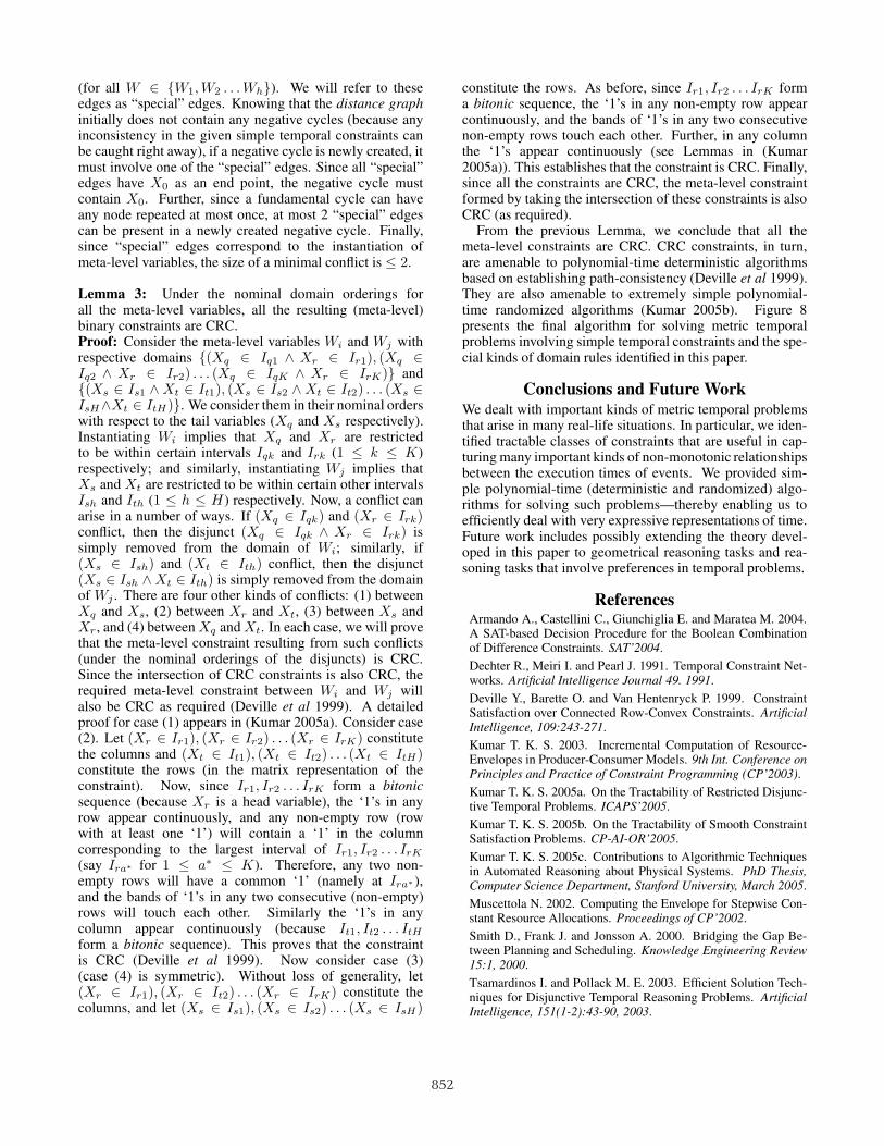
Lemma 3: Under the nominal domain orderings forall the meta-level variables, all the resulting (meta-level)binary constraints are CRC.Proof: Consider the meta-level variables Wi and Wj withrespective domains {(Xq ∈ Iq1 ∧ Xr ∈ Ir1), (Xq ∈Iq2 ∧ Xr ∈ Ir2) . . . (Xq ∈ IqK ∧ Xr ∈ IrK)} and{(Xs ∈ Is1 ∧ Xt ∈ It1), (Xs ∈ Is2 ∧ Xt ∈ It2) . . . (Xs ∈IsH∧Xt ∈ ItH)}. We consider them in their nominal orderswith respect to the tail variables (Xq and Xs respectively).Instantiating Wi implies that Xq and Xr are restrictedto be within certain intervals Iqk and Irk (1 ≤ k ≤ K)respectively; and similarly, instantiating Wj implies thatXs and Xt are restricted to be within certain other intervalsIsh and Ith (1 ≤ h ≤ H) respectively. Now, a conflict canarise in a number of ways. If (Xq ∈ Iqk) and (Xr ∈ Irk)conflict, then the disjunct (Xq ∈ Iqk ∧ Xr ∈ Irk) issimply removed from the domain of Wi; similarly, if(Xs ∈ Ish) and (Xt ∈ Ith) conflict, then the disjunct(Xs ∈ Ish ∧ Xt ∈ Ith) is simply removed from the domainof Wj . There are four other kinds of conflicts: (1) betweenXq and Xs, (2) between Xr and Xt, (3) between Xs andXr, and (4) between Xq and Xt. In each case, we will provethat the meta-level constraint resulting from such conflicts(under the nominal orderings of the disjuncts) is CRC.Since the intersection of CRC constraints is also CRC, therequired meta-level constraint between Wi and Wj willalso be CRC as required (Deville et al 1999). A detailedproof for case (1) appears in (Kumar 2005a). Consider case(2). Let (Xr ∈ Ir1), (Xr ∈ Ir2) . . . (Xr ∈ IrK) constitutethe columns and (Xt ∈ It1), (Xt ∈ It2) . . . (Xt ∈ ItH)constitute the rows (in the matrix representation of theconstraint). Now, since Ir1, Ir2 . . . IrK form a bitonicsequence (because Xr is a head variable), the ‘1’s in anyrow appear continuously, and any non-empty row (rowwith at least one ‘1’) will contain a ‘1’ in the columncorresponding to the largest interval of Ir1, Ir2 . . . IrK

(say Ira∗ for 1 ≤ a∗ ≤ K). Therefore, any two non-empty rows will have a common ‘1’ (namely at Ira∗ ),and the bands of ‘1’s in any two consecutive (non-empty)rows will touch each other. Similarly the ‘1’s in anycolumn appear continuously (because It1, It2 . . . ItH

form a bitonic sequence). This proves that the constraintis CRC (Deville et al 1999). Now consider case (3)(case (4) is symmetric). Without loss of generality, let(Xr ∈ Ir1), (Xr ∈ It2) . . . (Xr ∈ IrK) constitute thecolumns, and let (Xs ∈ Is1), (Xs ∈ Is2) . . . (Xs ∈ IsH)

constitute the rows. As before, since Ir1, Ir2 . . . IrK forma bitonic sequence, the ‘1’s in any non-empty row appearcontinuously, and the bands of ‘1’s in any two consecutivenon-empty rows touch each other. Further, in any columnthe ‘1’s appear continuously (see Lemmas in (Kumar2005a)). This establishes that the constraint is CRC. Finally,since all the constraints are CRC, the meta-level constraintformed by taking the intersection of these constraints is alsoCRC (as required).

From the previous Lemma, we conclude that all themeta-level constraints are CRC. CRC constraints, in turn,are amenable to polynomial-time deterministic algorithmsbased on establishing path-consistency (Deville et al 1999).They are also amenable to extremely simple polynomial-time randomized algorithms (Kumar 2005b). Figure 8presents the final algorithm for solving metric temporalproblems involving simple temporal constraints and the spe-cial kinds of domain rules identified in this paper.

Conclusions and Future WorkWe dealt with important kinds of metric temporal problemsthat arise in many real-life situations. In particular, we iden-tified tractable classes of constraints that are useful in cap-turing many important kinds of non-monotonic relationshipsbetween the execution times of events. We provided sim-ple polynomial-time (deterministic and randomized) algo-rithms for solving such problems—thereby enabling us toefficiently deal with very expressive representations of time.Future work includes possibly extending the theory devel-oped in this paper to geometrical reasoning tasks and rea-soning tasks that involve preferences in temporal problems.

ReferencesArmando A., Castellini C., Giunchiglia E. and Maratea M. 2004.A SAT-based Decision Procedure for the Boolean Combinationof Difference Constraints. SAT’2004.Dechter R., Meiri I. and Pearl J. 1991. Temporal Constraint Net-works. Artificial Intelligence Journal 49. 1991.Deville Y., Barette O. and Van Hentenryck P. 1999. ConstraintSatisfaction over Connected Row-Convex Constraints. ArtificialIntelligence, 109:243-271.Kumar T. K. S. 2003. Incremental Computation of Resource-Envelopes in Producer-Consumer Models. 9th Int. Conference onPrinciples and Practice of Constraint Programming (CP’2003).Kumar T. K. S. 2005a. On the Tractability of Restricted Disjunc-tive Temporal Problems. ICAPS’2005.Kumar T. K. S. 2005b. On the Tractability of Smooth ConstraintSatisfaction Problems. CP-AI-OR’2005.Kumar T. K. S. 2005c. Contributions to Algorithmic Techniquesin Automated Reasoning about Physical Systems. PhD Thesis,Computer Science Department, Stanford University, March 2005.Muscettola N. 2002. Computing the Envelope for Stepwise Con-stant Resource Allocations. Proceedings of CP’2002.Smith D., Frank J. and Jonsson A. 2000. Bridging the Gap Be-tween Planning and Scheduling. Knowledge Engineering Review15:1, 2000.Tsamardinos I. and Pollack M. E. 2003. Efficient Solution Tech-niques for Disjunctive Temporal Reasoning Problems. ArtificialIntelligence, 151(1-2):43-90, 2003.

852