Tracking for Augmented Reality on Wearable...
23
Tracking for Augmented Reality on Wearable Computers Ulrich Neumann and Jun Park Computer Science Department Integrated Media Systems Center University of Southern California {uneumann | junp}@graphics.usc.edu Abstract Wearable computers afford a degree of mobility that makes tracking for augmented reality difficult. This paper presents a novel object-centric tracking architecture for presenting augmented reality media in spatial relationships to objects, regardless of the objects’ positions or motions in the world. The advance this system provides is the ability to sense and integrate new features into its tracking database, thereby extending the tracking region automatically. A lazy evaluation of the structure from motion problem uses images obtained from a single calibrated moving camera and applies recursive filtering to identify and estimate the 3D positions of new features. We evaluate the performance of two filters; a classic Extended Kalman Filter (EKF) and a filter based on a Recursive-Average of Covariances (RAC). Implementation issues and results are discussed in conclusion. 1. Motivation and Introduction Wearable computers offer a compelling target for augmented reality (AR) interface metaphors. The promise of wearables is to endow users with essentially limitless mobility and range. Users, moving about and interacting with the real world, receive data
Transcript of Tracking for Augmented Reality on Wearable...

Tracking for Augmented Reality on Wearable Computers
Ulrich Neumann and Jun Park
Computer Science Department
Integrated Media Systems Center
University of Southern California
{uneumann | junp}@graphics.usc.edu
Abstract
Wearable computers afford a degree of mobility that makes tracking for augmented
reality difficult. This paper presents a novel object-centric tracking architecture for
presenting augmented reality media in spatial relationships to objects, regardless of the
objects’ positions or motions in the world. The advance this system provides is the
ability to sense and integrate new features into its tracking database, thereby extending
the tracking region automatically. A lazy evaluation of the structure from motion
problem uses images obtained from a single calibrated moving camera and applies
recursive filtering to identify and estimate the 3D positions of new features. We evaluate
the performance of two filters; a classic Extended Kalman Filter (EKF) and a filter based
on a Recursive-Average of Covariances (RAC). Implementation issues and results are
discussed in conclusion.
1. Motivation and Introduction
Wearable computers offer a compelling target for augmented reality (AR) interface
metaphors. The promise of wearables is to endow users with essentially limitless
mobility and range. Users, moving about and interacting with the real world, receive data

and communication through wearables. The AR metaphor of overlaying information in
spatial relationships to real objects support such interactions without the ambiguity that
may arise from text or diagrams displayed in fixed screen positions. Figure 1 illustrates
how spatially aligned AR overlays can concisely communicate information and tasks.
Maintaining the spatial alignment between virtual annotation and real objects as users
move requires dynamic tracking of the viewpoint relative to objects.
Fig. 1 Example of AR annotation supporting a
maintenance task
Tracking has been at the heart of research and development in augmented reality (AR)
since it’s inception in the 1960’s [SUTH68]. Many systems have been developed to track
the six-degree of freedom (6DOF) pose of an object (or a person) relative to a fixed
coordinate-frame in the environment [FOXL96, GHAZ95, KIM97, MEYE92, SOWI93,
STAT96, WARD92, WELC97]. These tracking systems employ a variety of sensing
technologies, each with unique strengths and weaknesses, to determine a world-centric
pose measurement, as required for virtual and augmented reality applications. Tracking
for AR in a fixed frame of reference, however, implies that objects in the environment are
calibrated to the tracker’s frame of reference and that, after calibration they remain fixed.
This assumption is valid for applications such as architectural visualization [KLIN97,
FEIN95] where the walls and floors form a rigid structure whose world coordinates can
be calibrated, or are already known by design, and are not likely to move. World-centric
trackers can be used to calibrate movable objects [FEIN93, STAR97, WELL93,
BAJU92], but this generally entails placing and calibrating tracking system elements on
each object of interest and operating within range of the shared tracking infrastructure,
(e.g., magnetic fields or active beacons) [KIM97, WELC97]. These requirements make it
difficult and expensive to accommodate moving objects with current world-centric
tracking approaches.
A large class of AR applications require annotation on objects whose positions in a room
or the world may vary freely without impact on the AR media linked to them. For
example, AR applications in manufacturing, maintenance, and training [KLIN97,
CAUD92, FEIN93] require virtual annotations that provide task guidance and specific
component indications on subassemblies or portions of structure (Fig.1). These
applications are particularly suited to wearable computers because of the mobility
afforded to the user. A more appropriate tracking solution for these highly mobile
applications is one that is object-centric, or in other words, based on viewing the object
itself [NATO95, NEUM96, REKI97, SHAR97, UENO95, STAR97, KUTU96,
MELL95]. Such tracking is possible with the pose estimation methods developed in the
fields of computer vision and photogrammetry [HUAN94, FISC81]. However, a
weakness of vision-based tracking is that pose is only computed for those views that
contain known features of the scene. Given the mobility of wearable computer users, and
the range of tasks they may need to perform, it is necessary to increase the robustness of
pose tracking. Our tracking method can dynamically expand the range and robustness of
tracked AR camera views as the system is operating.
1.1. Issues in Vision-Based Tracking
Vision-based tracking is the problem of calibrating a camera’s pose relative to an object,
given one or more images. Vision-based tracking methods can be roughly grouped into
the three following categories, based on their requirements:
♦ Three or more known 3D points from a single image [FISC81, GANA84, HORA89,
KLIN97, KUTU96, MELL95, SHAR97, NEUM96, WARD92]
♦ A sequence of images from a moving camera where point positions may be known or
unknown [AZAR95, BROI90, SOAT94, WELC97, UENO95]
♦ Model and template matching from a single image [LU96 , NATO95]
The first class of approaches uses a calibrated camera to provide constraints to the pose
formulation, so only a few known points within a single image are needed for tracking.
This class of methods has been successfully employed in AR tracking systems, and it is
used in our system as well.
The points needed for tracking can be object features such as corners and holes, or they
can be intentionally designed and applied targets or fiducials. We selected the latter
option in our work since naturally-occurring features can be difficult to recognize due to
their variety and unpredictable characteristics. Also, objects do not always have features
where they are needed for tracking; large regions of surfaces are often indistinguishable
when viewed without context. Fiducials have the advantage that they can be designed to
maximize the AR system’s ability to detect and distinguish between them, they can be
inexpensive, and they can be placed arbitrarily on objects. The design and detection of

fiducials are important topics, but in this work, we assume only that fiducials have some
basic characteristics such as color and shape.
Our goal is to increase the range of camera-motion that provides tracked viewing while
minimizing the number of fiducials that must be applied to an object. A worst-case
occurs when all regions of a large object are equally likely to be viewed and therefore a
dense distribution of fiducials is needed to support tracking over the entire object.
Covering large objects (e.g., airplanes, machinery) with fiducials is impractical and
calibrating them is difficult. Our approach is an alternative analogous to “lazy-
evaluation” in algorithm design; fiducials are only placed, and their positions computed,
as the need for them arises. An initial set of fiducials is strategically placed and
calibrated on an object or a fixture rigidly connected to an object. As regions of the
object require additional fiducials to support tracking, users simply add new fiducials to
those regions of interest and allow the system to automatically calibrate them. Once
calibrated, the new fiducials are added to the database of known fiducials that are used
for tracking. In addition to extending the range of tracked poses, the additional fiducials
stabilize the pose calculation since more fiducials are likely to be visible in images.
This approach is most practical when a limited region of the object needs to be viewed
and tracked for a given task, but that region and task is just one of many that may occur.
Assembly, training, and maintenance tasks often have this quality. Information for a
given task is local, but the specific task and locality is only one of many that may be
performed by different people at different times. Figure 1 illustrates AR annotation for a
maintenance task that requires tracking in only a limited region around an access panel in
a larger structure.

The remainder of this paper presents our vision-based AR tracking architecture. Details
are given on the recursive filters that calibrate the 3D positions of new fiducials. We
compare the results from two filters and two operational examples.
2. System Architecture
Figure 2 depicts our architecture. A single camera provides real time video input, and a
user observes the camera image and AR media overlay on a display that may be desktop,
handheld, or head-mounted. Sections 2.1 - 2.3 describe the components of this
architecture that set the context for section 3 where the unique new point evaluation is
described.
cameravideo
segmentation andfeature detection
identifiedfiducials
2D correspondence
correspondedfiducials
(R, p, q)
uncorresponded fiducials (p, q)
6 DOF camera pose
3D correspondence
rankedposes K
3D Object fiducial DB(color, shape, position)
3D New fiducial DB(color, shape, position)
render 3D graphics
confirmedpose K
displayvideo
3D position update
new objectfiducials(R, q)
fiducial traits (R, q)
candidatefiducials
fiducial traits (R, q)
estimate (R, I)
(p, q)
(p, q)
Fig. 2 - AR system architecture for extendible vision-
based tracking. New fiducial management functions are
shown against a gray background

2.1. Segmentation and Feature Detection
The important aspect of this step is that fiducials must be robustly detected and located.
They are defined by a 2D screen position p and a type q that encodes characteristics such
as color and shape. Our fiducial design is a colored circle or triangle [NEUM96], but
other designs such as concentric circles or coded squares are equally valid [STAT96,
EAGL, KLIN97, MELL95]. We use the three primary and three secondary colors along
with the triangle and circle shapes to provide twelve unique fiducial types. Fiducials are
detected by segmenting the image into regions of similar intensity and color and testing
the regions for the color and geometric properties of fiducials. Detection strategies are
often dependent on the characteristics of the fiducials [REKI97, TREM97, UENO95].
2.2. 2D Correspondence
The 2D fiducials (p,q) must be corresponded to elements in a database of known 3D
fiducial positions and types(R,q). The result of a successful match is a corresponded
fiducial whose 2D screen position and 3D coordinate on the object are now known
(R,p,q). Fiducials observed in the image, but not corresponded to the world database, are
passed on as uncorresponded fiducials and potential new points to estimate.
Computing correspondences is hard in the general case [MELL95, UENO95], and trivial
if the fiducial types are unique for each element in the database. For this work, we
consider only unique feature types that are trivial to correspond since our focus is on the
extendible tracking portion of the architecture, however, we recognize that
correspondence is a necessary function for the architecture to scale to truly useful levels.

Other researchers have proposed solutions of varying applicability to our case, and we
intend to leverage from their work in the future [SHAR97, MELL95].
2.3. Camera Pose
Three or more corresponded fiducials allows the camera pose to be determined [FISC81].
The approach we use has known instabilities in certain poses, and in general provides
multiple solutions (two or four) from a fourth-degree polynomial. Methods have been
proposed to select the most likely solution [SHAR97]. We weight several tests to rank
the possible pose solutions in terms of their apparent correctness.
♦ The distance between the current and last frame’s viewpoint is inversely proportional
to a solution’s weight.
♦ The fiducials’ relative pixel-areas are tested for agreement with the expected
relationships based on each pose solution.
♦ When more than three known fiducials are available, their projections under the
candidate poses are compared to their measured positions.
♦ When more than three known fiducials are available multiple pose calculations are
performed for different sets of three fiducials, and the closest pairs from each
calculation are highly ranked.
The result of this function is an array of poses K, ranked by the above tests, which are
passed on to the new point functions (shown over gray in Fig. 2).
3. New Point Evaluation
This section details the unique aspects of this architecture that provide the interactive
extension of the tracked viewing range. Given the camera pose and image coordinates of

the uncorresponded features, these features’ position estimates are updated in one or two
possible ways, as detailed in the next section.
3.1. Algorithms
3.1.1. Initial Estimates
For uncorresponded fiducials (p, q), the intersection1 of two lines connecting the camera
positions and the fiducial locations in the image create the initial estimate of the 3D
position of the fiducial. The intersection threshold is scaled to the expected size of the
fiducials. For example, if the radius of the fiducials is 0.5 inch, as in our case, the
threshold is 1.0 inch. Our selection is based on the minimum distance that two distinct
fiducials can be placed without overlap. Lines with a closest point of approach less than
1.0 inch are considered to be intersecting.
3.1.2. Extended Kalman Filter (EKF)
The Extended Kalman Filter (EKF) has been used in many applications, and details of the
method can be found in references such as [MEND95, WELC97, BROI90].
Inputs to the EKF are the current camera pose and the image coordinates of the fiducial.
kc : camera pose at kth time step
kz : image coordinates of the fiducial at kth time step
The state of the EKF is the current estimate of the fiducial’s 3D position. The real 3D
position of the fiducial is constant over time, so no dynamics are involved in the KEF
1 Since two lines in 3D space may not actually intersect, the point midway between the
points of closest approach is used as the intersection.
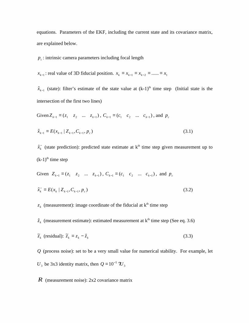
equations. Parameters of the EKF, including the current state and its covariance matrix,
are explained below.
cp : intrinsic camera parameters including focal length
1−kx : real value of 3D fiducial position. 121 ...... xxxx kkk ==== −−
1ˆ −kx (state): filter’s estimate of the state value at (k-1)th time step (Initial state is the
intersection of the first two lines)
Given )...( 1211 −− = kk zzzZ , )...( 1211 −− = kk cccC , and cp
),,|(ˆ 1111 ckkkk pCZxEx −−−− = (3.1)
−kx (state prediction): predicted state estimate at kth time step given measurement up to
(k-1)th time step
Given )...( 1211 −− = kk zzzZ , )...( 1211 −− = kk cccC , and cp
),,|(ˆ 11 ckkkk pCZxEx −−− = (3.2)
kz (measurement): image coordinate of the fiducial at kth time step
kz (measurement estimate): estimated measurement at kth time step (See eq. 3.6)
kz~ (residual): kkk zzz ˆ~ −= (3.3)
Q (process noise): set to be a very small value for numerical stability. For example, let
3U be 3x3 identity matrix, then 3510 UQ ?= −
R (measurement noise): 2x2 covariance matrix

Let 2U be 2x2 identity matrix, then 22 UR ?= , assuming that the measurement error
variance is 2, and there is no correlation between x and y coordinates in the image space.
1−kP (state uncertainty): 3x3 uncertainty covariance matrix at (k-1)th time step
])ˆ)(ˆ[( 11111T
kkkkk xxxxEP −−−−− −−= (3.4)
−kP (state uncertainty prediction): predicted state uncertainty at kth time step given
measurement up to (k-1)th time step
])ˆ)(ˆ[( Tkkkkk xxxxEP −−− −−= (3.5)
hr
(measurement function): function returning the projection(measurement estimate) of
the current position estimate given the current camera pose and camera parameters
),,ˆ(ˆ ckkk pcxhz −=r
(3.6)
kH (Jacobian): Jacobian matrix of hr
kK (Kalman Gain): 3x2 matrix. See equation (3.9)
The EKF process is composed of two groups of equations: predictor(time update) and
corrector(measurement update). The predictor updates the previous ((k-1) th) state and its
uncertainty to the predicted values at the current (kth) time step. Since the 3D fiducial
position does not change with time, the predicted position at the current time step is the
same as the position of the previous time step.
),,ˆ(ˆ
ˆˆ
1
1
ckkk
kk
kk
pcxhz
QPP
xx
−
−−
−−
=
+=
=
r
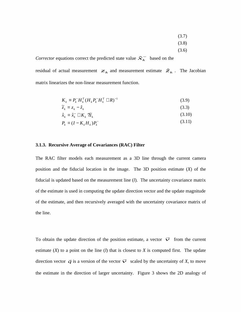
Corrector equations correct the predicted state value −kx based on the
residual of actual measurement kz and measurement estimate kz . The Jacobian
matrix linearizes the non-linear measurement function.
3.1.3. Recursive Average of Covariances (RAC) Filter
The RAC filter models each measurement as a 3D line through the current camera
position and the fiducial location in the image. The 3D position estimate (X) of the
fiducial is updated based on the measurement line (l). The uncertainty covariance matrix
of the estimate is used in computing the update direction vector and the update magnitude
of the estimate, and then recursively averaged with the uncertainty covariance matrix of
the line.
To obtain the update direction of the position estimate, a vector vr
from the current
estimate (X) to a point on the line (l) that is closest to X is computed first. The update
direction vector qr is a version of the vector v
r scaled by the uncertainty of X, to move
the estimate in the direction of larger uncertainty. Figure 3 shows the 2D analogy of
)6.3(
)8.3(
)7.3(
−
−
−−−
−=
?+=
−=+=
kkkk
kkkk
kkk
Tkkk
Tkkk
PHKIP
zKxx
zzz
RHPHHPK
)(
~ˆˆ
ˆ~)( 1
)11.3(
)10.3(
)3.3(
)9.3(
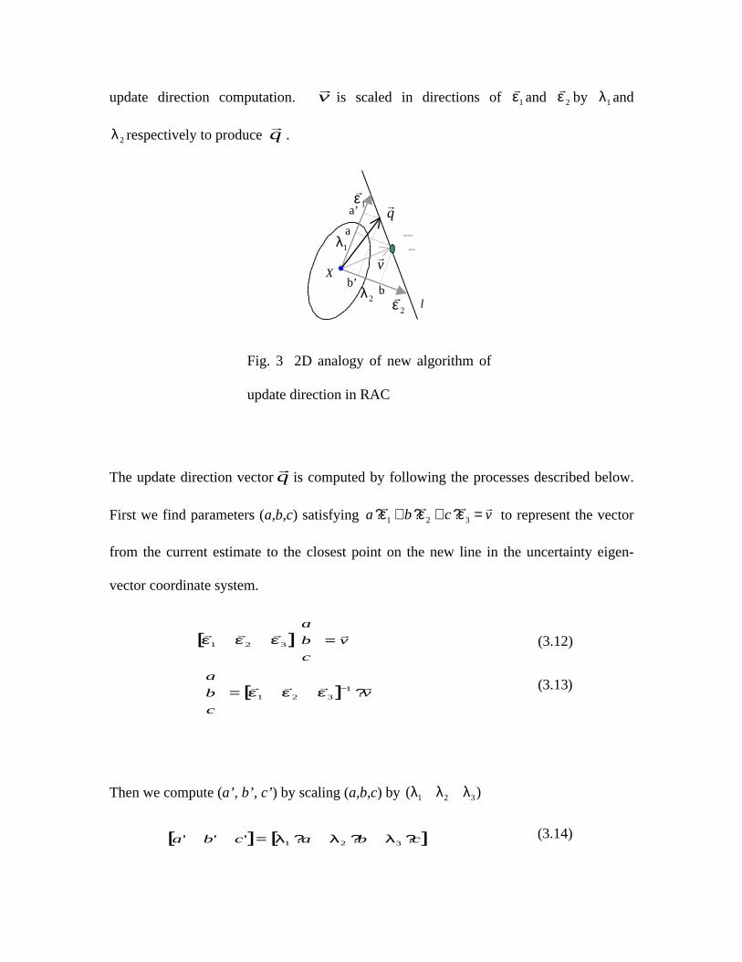
update direction computation. vr
is scaled in directions of 1εr and 2εr by 1λ and
2λ respectively to produce qr
.
1εr
2εr
1λ
2λ
Closest
point
vr
qr
a
b
a’
b’X
l
Fig. 3 2D analogy of new algorithm of
update direction in RAC
The update direction vector qr
is computed by following the processes described below.
First we find parameters (a,b,c) satisfying vcbarrrr =?+?+? 321 εεε to represent the vector
from the current estimate to the closest point on the new line in the uncertainty eigen-
vector coordinate system.
Then we compute (a’, b’, c’) by scaling (a,b,c) by )( 321 λλλ
[ ]
[ ] v
c
b
a
v
c
b
a
rrrr
rrrr
?=���
�
�
���
�
�
=���
�
�
���
�
�
−1321
321
εεε
εεε
)13.3(
)12.3(
[ ] [ ]cbacba ???= 321''' λλλ )14.3(

Finally, the update direction qr
is obtained using the scaled components (a’, b’, c’).
The update magnitude m of the position estimate is
m = min(du, dl)
where du is the uncertainty of the current estimate in the direction of qr
and dl is the
scaled distance from X to l in the direction of qr
,i.e., qr
.
The uncertainty of the position estimate is represented by a 3x3 covariance matrix. Each
line has a constant uncertainty kL , which is narrow and long along the direction of the
line. Uncertainty is updated by recursively averaging the covariance matrices, similar to
the process used in the Kalman Filter. In the Kalman Filter, the uncertainty covariance
matrix is updated by performing weighted-averaging with 2D-measurement error
covariance as below.
In the RAC filter, the measurement is modeled as a line that is already in the same 3D
space the estimate is in. Therefore we can eliminate the Jacobian matrix and its
linearization approximation. This is an advantage of the RAC filter over the EKF,
simplifying and reducing the computational overhead. Let −kP be the uncertainty
321 ''' εεεrrrr ?+?+?= cbaq )15.3(
)16.3(
−
−−−
−=
+=
kkkk
kTkkk
Tkkk
PHKIP
RHPHHPK
)(
)( 1
)11.3(
)9.3(

covariance matrix of the current estimate and kL be that of the new line, then
computation of the updated uncertainty covariance matrix kP is simplified as below.
The initial value of kP is obtained in the same way by replacing −kP with kL ,
resulting from the two initial line uncertainties.
3.2. Experiment and Result
Both filters appear stable in practice. The EKF is known to have good characteristics
under certain conditions [BROI90], however the RAC gives comparable results, and it is
simpler, operating completely in 3D world space with 3D lines as measurements. The
RAC approach eliminates the linearization processes required in the EKF with Jacobian
matrices.
We tested the EKF and RAC filters to find the positions of two new fiducials (refered to
as red and magenta fiducials). We started with three known fiducials and two cases were
tested. In the panning case, new fiducials were placed to the side of the known fiducials,
assuming a translated region of interest. In the zooming case, new fiducials were placed
in the center so that the user could zoom in to a region of interest.
−−−
−−−−−−−
−−−−
−
−−−
+=
+−++=
+−=
−=
+=
kkkk
kkkkkkkk
kkkk
kkk
kkkk
PLPL
PLPPLPLP
PLPPI
PKIP
LPPK
))((
))())(((
))((
)(
)(
1
11
1
1
)21.3(
)20.3(
)19.3(
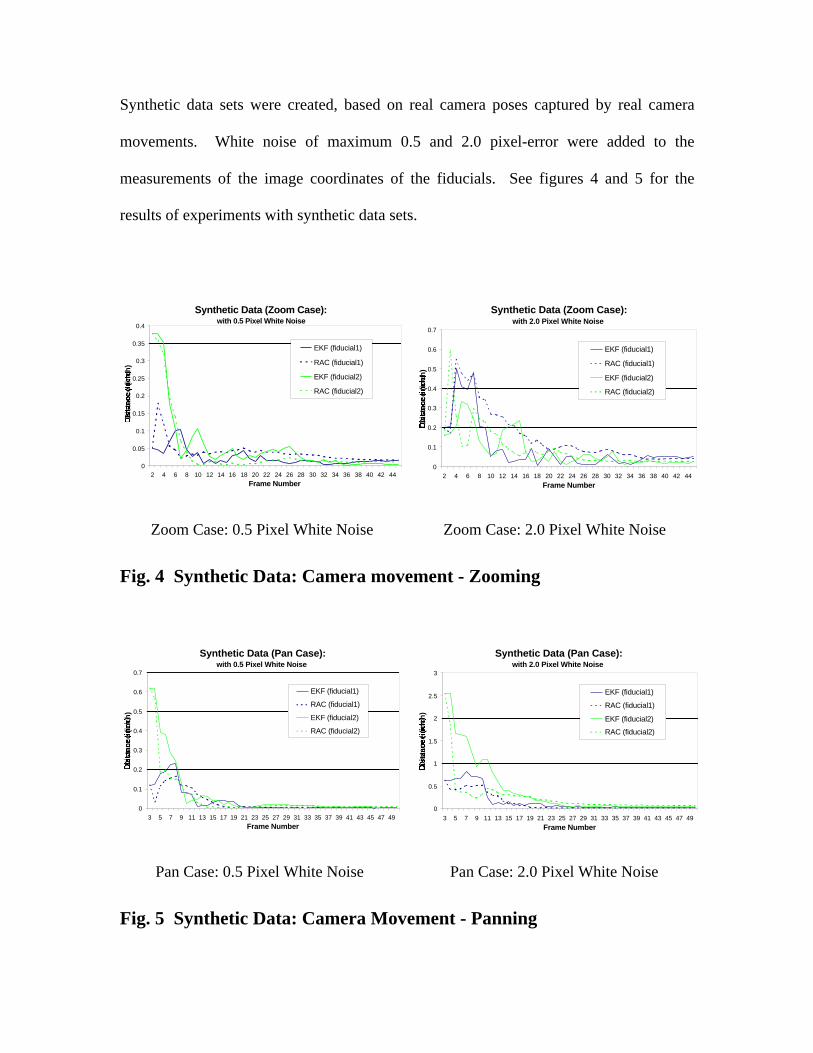
Synthetic data sets were created, based on real camera poses captured by real camera
movements. White noise of maximum 0.5 and 2.0 pixel-error were added to the
measurements of the image coordinates of the fiducials. See figures 4 and 5 for the
results of experiments with synthetic data sets.
Synthetic Data (Zoom Case): with 0.5 Pixel White Noise
0
0.05
0.1
0.15
0.2
0.25
0.3
0.35
0.4
2 4 6 8 10 12 14 16 18 20 22 24 26 28 30 32 34 36 38 40 42 44
Frame Number
Dis
tan
ce (
inch
)
EKF (fiducial1)
RAC (fiducial1)
EKF (fiducial2)
RAC (fiducial2)
Synthetic Data (Zoom Case): with 2.0 Pixel White Noise
0
0.1
0.2
0.3
0.4
0.5
0.6
0.7
2 4 6 8 10 12 14 16 18 20 22 24 26 28 30 32 34 36 38 40 42 44
Frame Number
Dis
tan
ce (
inch
)
EKF (fiducial1)
RAC (fiducial1)
EKF (fiducial2)
RAC (fiducial2)
Zoom Case: 0.5 Pixel White Noise Zoom Case: 2.0 Pixel White Noise
Fig. 4 Synthetic Data: Camera movement - Zooming
Synthetic Data (Pan Case): with 0.5 Pixel White Noise
0
0.1
0.2
0.3
0.4
0.5
0.6
0.7
3 5 7 9 11 13 15 17 19 21 23 25 27 29 31 33 35 37 39 41 43 45 47 49
Frame Number
Dis
tan
ce (
inch
)
EKF (fiducial1)
RAC (fiducial1)
EKF (fiducial2)
RAC (fiducial2)
Synthetic Data (Pan Case): with 2.0 Pixel White Noise
0
0.5
1
1.5
2
2.5
3
3 5 7 9 11 13 15 17 19 21 23 25 27 29 31 33 35 37 39 41 43 45 47 49
Frame Number
Dis
tan
ce (
inch
)
EKF (fiducial1)
RAC (fiducial1)
EKF (fiducial2)
RAC (fiducial2)
Pan Case: 0.5 Pixel White Noise Pan Case: 2.0 Pixel White Noise
Fig. 5 Synthetic Data: Camera Movement - Panning

Experiments with real data were performed in both the zoom and pan cases (figure 7).
The estimates of the filters were compared with analytic solutions, which have the
minimum sum of Euclidean distances to the input lines. Figure 6 shows a 2D analogy of
the analytic solution computation.
l4
l3
l2
l1
d4
d3d2
d1
X
Fig. 6 2D Analogy of Analytic Solution:
The analytic solution is a point that has minimum sum
of distances to the lines. In this case, the analytic
solution is a point X that minimizes d1+ d2+ d3+ d4.
Real Data (Zoom Case)
0
0.1
0.2
0.3
0.4
0.5
0.6
0.7
0.8
2 4 6 8 10 12 14 16 18 20 22 24 26 28 30 32 34 36 39 42
Frame Number
Dis
tan
ce (
inch
)
EKF (red fiducial)
RAC (red fiducial)
EKF (magenta fiducial)
RAC (magenta fiducial)
Real Data (Pan Case)
0
0.5
1
1.5
2
2.5
3
3.5
3 5 7 9 11 13 16 18 20 22 24 26 28 30 32 34 36 38 40 42 44
Frame Number
Dis
tan
ce (
inch
)
EKF (red fiducial)
RAC (red fiducial)
EKF (magenta fiducial)
RAC (magenta fiducial)
Zoom Case Pan Case
Fig. 7 Real Data: Zooming and Panning cases

A virtual camera view shows the results of the real data experiments graphically (figure
8). The lines are traces of the camera, i.e., the input lines used for RAC filter. The large
spheres indicate positions of known fiducials, which were used for computing camera
poses. The dark and bright small spheres represent the estimated positions produced by
the RAC and EKF filters, while the black cube represents the analytic solution positions.
Pan Case: Magenta fiducial
The EKF result (bright sphere) appears in
front of the analytic solution (black cube),
and the RAC filter result (dark sphere) is
just to their left.
Zoom Case: Red fiducial
The EKF result (bright sphere), RAC filter
result (dark sphere), and the analytic solution
(black cube) overlap and are not separately
discernible.
Fig. 8 Virtual camera views of the results of real data experiments.
The results show that the estimates of the filters converge fast and remain stable after
convergence with both real and synthetic data.
Our hardware configuration included a desktop workstation, however this system is
similar in computing power to currently available portable laptops or wearables.
♦ SGI Indy 24-bit graphics system with MIPS4400@200MHz.
♦ SONY DXC-151A color video camera with 640x480 resolution, 31.4 degree
horizontal and 24.3 degree vertical field of view (FOV), S-video output.
Our future work entails a solution to the 2D correspondence problem. This is necessary
for the system to scale to greater numbers of fiducials. We also hope to improve our
ability to select the correct pose solution, and we will have to address the error
propagation from multiple chained fiducial estimates.
4.0 Acknowledgments
We gratefully acknowledge support funding from NSF grant CCR-9502830 and the
Integrated Media Systems Center, a National Science Foundation Engineering Research
Center with additional support from the Annenberg Center for Communication at the
University of Southern California and the California Trade and Commerce Agency. Our
thanks also go to Youngkwan Cho, Suya You, Anthony Majoros (The Boeing Co.), and
Michael Bajura (Interval Corp.) for technical input.
5.0 References
[AZAR95] A. Azarbayejani, A. Pentland, “Recursive Estimation of Motion, Structure, and Focal Length,”
IEEE Transactions on Pattern Analysis and Machine Intelligence, Vol. 17, No. 6, June 1995
[BAJU92] Bajura, M., Fuchs, H., Ohbuchi, R. "Merging Virtual Reality with the Real World: Seeing
Ultrasound Imagery within the Patient," Computer Graphics (Proceedings of Siggraph 1992), pp. 203-
210.
[BROI90] T. J. Broida, S. Chandrashekhar, R. Chellappa, “Recursive Estimation from a Monocular Image
Sequence,” IEEE Transactions on Aerospace and Electronic Systems, Vol. 26, No. 4, pp. 639-655, July
1990
[CAUD92] T. P. Caudell, D. M. Mizell, “Augmented Reality: An Application of Heads-Up Display
Technology to Manual Manufacturing Processes,” Proceedings of the Hawaii International Conference
on Systems Sciences, pp. 659-669, 1992
[EAGL] Eagle Eye, Kinetic Sciences http://www.kinetic.bc.ca/eagle_eye.html
[FEIN93] S. Feiner, B. MacIntyre, D. Seligmann, “Knowledge-Based Augmented Reality,”
Communications of the ACM, Vol. 36, No. 7, pp 52-62, July 1993
[FEIN95] S. Feiner, A. Webster, T Krueger III, M MacIntyre, E. Keller, “Architectural Anatomy,”
Presence: Teleoperator and Virtual Environments, Vol. 4, No. 3, pp. 318-325, Summer 1995
[FISC81] Fischler, M.A., Bolles, R.C. “Random Sample Consensus: A Paradigm for Model Fitting with
Applications to Image Analysis and Automated Cartography,” Graphics and Image Processing, Vol.
24, No. 6, 1981, pp. 381-395.
[FOXL96] E. Foxlin, “Inertial Head-Tracker Sensor Fusion by a Complementary Separate-Bias Kalman
Filter,” Proceedings of VRAIS’96, pp. 184-194
[GANA84] S. Ganapathy, “Real-Time Motion Tracking Using a Single Camera,” AT&T Bell Labs Tech
Report 11358-841105-21-TM, Nov. 1984

[GHAZ95] M. Ghazisadedy, D. Adamczyk, D. J. Sandlin, R. V. Kenyon, T. A. DeFanti, “Ultrasonic
Calibration of a Magnetic Tracker in a Virtual Reality Space,” Proceedings of VRAIS’95, pp. 179-188
[HORA89] R. Horaud, B. Conio, O. Leboulleux, “An Analytic Solution for the Perspective 4-point
Problem,” Compter Vision, Graphics, and Image Processing, Vol. 47, No. 1, pp. 33-43, 1989
[HUAN94] T. S. Huang, A. N. Netravali, “Motion and Structure from Feature Correspondences: A
Review,” Proceedings of the IEEE, Vol. 82, No. 2, pp. 252-268, Feb. 1994
[KIM97] D. Kim, S. W. Richards, T. P. Caudell, “An Optical Tracker for Augmented Reality and
Wearable Computers,” Proceedings of VRAIS’97, pp. 146-150
[KLIN97] G. Klinker, K. Ahlers, D. Breem, P. Chevalier, C. Crampton, D. Greer, D. Koller, A. Kramer, E.
Rose, M. Tuceryan, R. Whitaker, “Confluence of Computer Vision and Interactive Graphics for
Augmented Reality,” Presence: Teleoperator and Virtual Environments, Vol. 6, No. 4, pp. 433-451,
August 1997
[KUTU96] K. Kutulakos, J. Vallino, “Affine Object Representations for Calibration-Free Augmented
Reality,” Proceedings of VRAIS’96, pp. 25-36
[LU96] S-L. Iu, K. W. Rogovin, “Registering Perspective Contours with 3-D Objects without
Correspondence, Using Orthogonal Polynomials,” Proceedings of VRAIS’96, pp. 37-44
[MELL95] J. P. Mellor, “Enhanced Reality Visualization in a Surgical Environment,” Master’s Thesis,
Dept. of Electrical Engineering, MIT, 1995
[MEND95] J.M. Mendel, “Lessons in Estimation Theory for Signal Processing, Communications, and
Control”, Prentice Hall PTR, 1995
[MEYE92] K. Meyer, H. L. Applewhite, F. A. Biocca, “A Survey of Position Trackers,” Presence:
Teleoperator and Virtual Environments, Vol. 1, No. 2, pp. 173-200, 1992
[NATO95] E. Natonek, Th. Zimmerman, L. Fluckiger, “ Model Based Vision as Feedback for Virtual
Reality Robotics Environments,” Proceedings of VRAIS’95, pp. 110-117
[NEUM96] U. Neumann, Y. Cho, “A Self-Tracking Augmented Reality System,” Proceedings of ACM
Virtual Reality Software and Technology ‘96, pp. 109-115
[REKI97] J. Rekimoto, “NaviCam: A Magnifying Glass Approach to Augmented Reality,” Presence:
Teleoperator and Virtual Environments, Vol. 6, No. 4, pp. 399-412, August 1997
[SHAR97] R. Sharma, J. Molineros, “Computer Vision-Based Augmented Reality for Guiding Manual
Assembly,” Presence: Teleoperator and Virtual Environments, Vol. 6, No. 3, pp. 292-317, June 1997
[SOAT94] S. Soatto, P. Perona, “Recursive 3D Visual Motion Estimation Using Subspace Constraints,”
CIT-CDS 94-005, California Institute of Technology, Tech Report, Feb. 1994
[SOWI93] H. Sowizral, J. Barnes, “Tracking Position and Orientation in a Large Volume,” Proceedings of
IEEE VRAIS’93, pp. 132-139
[STAR97] T. Starner, S. Mann, B. Rhodes, J. Levine, J. Healey, D. Kirsh, R. Picard, A. Pentland,
“Augmented Reality Through Wearable Computing,” Presence: Teleoperator and Virtual Environments,
Vol. 6, No. 4, pp. 386-398, August 1997
[STAT96] A. State, G. Hirota, D. T. Chen, B. Garrett, M. Livingston, “Superior Augmented Reality
Registration by Integrating Landmark Tracking and Magnetic Tracking,” Proceedings of Siggraph96,
Computer Graphics, pp. 429-438
[SUTH68] I. Sutherland “A Head-Mounted Three-Dimensional Display,” Fall Joint Computer
Conference, pp. 757-775, 1968
[TREM97] A. Tremeau, N. Borel, “A Region Growing and Merging Algorithm to Color Segmentation,”
Pattern Recognition, Vol. 30, No. 7, pp. 1191-1203, 1997
[UENO95] M. Uenohara, T. Kanade, “Vision-Based Object Registration for Real-Time Image Overlay,”
Proceedings of Computer Vision, Virtual Reality, and Robotics in Medicine, pp. 13-22, 1995

[WARD92] M. Ward, R. Azuma, R. Bennett, S. Gottschalk, H. Fuchs, “A Demonstrated Optical Tracker
with Scalable Work Area for Head-Mounted Display Systems,” Proceedings of the 1992 Symposium
on Interactive 3D Graphics,” pp. 43-52
[WELC97] G. Welch, G. Bishop, “SCAAT: Incremental Tracking with Incomplete Information,”
Proceedings of Siggraph97, Computer Graphics, pp. 333-344
[WELL93] Wells, W., Kikinis, R., Altobelli, D., Ettinger, G., Lorensen, W., Cline, H., Gleason, P.L., and
Jolesz, F. “Video Registration Using Fiducials for Surgical Enhanced Reality,” Engineering in
Medicine and Biology, IEEE, 1993