Tracing semantic change with Latent Semantic Analysis · 2 Tracing semantic change with Latent...
32
Tracing semantic change with Latent Semantic Analysis Eyal Sagi Stefan Kaufmann Brady Clark Abstract: Research in historical semantics relies on the examination, selec- tion, and interpretation of texts from corpora. Changes in meaning are tracked through the collection and careful inspection of examples that span decades and centuries. This process is inextricably tied to the researcher‟s expertise and familiarity with the corpus. Consequently, the results tend to be difficult to quantify and put on an objective footing, and “big-picture” changes in the vocabulary other than the specific ones under investigation may be hard to keep track of. In this paper we present a method that uses Latent Semantic Analysis (Landauer, Foltz & Laham, 1998) to automatical- ly track and identify semantic changes across a corpus. This method can take the entire corpus into account when tracing changes in the use of words and phrases, thus potentially allowing researchers to observe the larger context in which these changes occurred, while at the same time considerably reducing the amount of work required. Moreover, because this measure relies on readily observable co-occurrence data, it affords the study of semantic change a measure of objectivity that was previously dif- ficult to attain. In this paper we describe our method and demonstrate its potential by applying it to several well-known examples of semantic change in the history of the English language. Keywords: Latent Semantic Analysis, Historical Linguistics, Semantic Change
Transcript of Tracing semantic change with Latent Semantic Analysis · 2 Tracing semantic change with Latent...

Tracing semantic change with Latent Semantic
Analysis
Eyal Sagi
Stefan Kaufmann
Brady Clark
Abstract: Research in historical semantics relies on the examination, selec-
tion, and interpretation of texts from corpora. Changes in meaning are
tracked through the collection and careful inspection of examples that span
decades and centuries. This process is inextricably tied to the researcher‟s
expertise and familiarity with the corpus. Consequently, the results tend to
be difficult to quantify and put on an objective footing, and “big-picture”
changes in the vocabulary other than the specific ones under investigation
may be hard to keep track of. In this paper we present a method that uses
Latent Semantic Analysis (Landauer, Foltz & Laham, 1998) to automatical-
ly track and identify semantic changes across a corpus. This method can
take the entire corpus into account when tracing changes in the use of
words and phrases, thus potentially allowing researchers to observe the
larger context in which these changes occurred, while at the same time
considerably reducing the amount of work required. Moreover, because this
measure relies on readily observable co-occurrence data, it affords the
study of semantic change a measure of objectivity that was previously dif-
ficult to attain. In this paper we describe our method and demonstrate its
potential by applying it to several well-known examples of semantic
change in the history of the English language.
Keywords: Latent Semantic Analysis, Historical Linguistics, Semantic
Change
2 Tracing semantic change with Latent Semantic Analysis
1 Introduction
The widespread availability of affordable and powerful computational ma-
chinery for the storage, manipulation and analysis of large data sets has had
a profound methodological impact on virtually every area of scholarly in-
quiry. Historical linguistics is no exception to this trend. This is not surpris-
ing inasmuch as the diachronic study of language has always relied on the
analysis of large amounts of text. But it is an exciting development none-
theless because the new computational tools open up methodological possi-
bilities that were hitherto unavailable. We see three major ways in which
research in historical linguistics has already been affected and will continue
to be transformed by data-driven computational methods. First, they pro-
vide an objective means to make observations and test hypotheses in a way
that does not depend on the researcher‟s intuitive judgment. Second, phe-
nomena which manifest themselves as statistical trends in large corpora can
be observed and quantified precisely and efficiently without enormous in-
vestments in manpower. Third, these methods have the potential to help
detect interesting trends in the data based on large-scale observations on the
entire corpus.
To be sure, computational methods have only just begun to have an im-
pact in historical linguistics. At this point, most work in the area is explora-
tory, testing and refining methods rather than putting them to work to pro-
duce new findings. This is also true for the work described in the present
paper. Our goal is to demonstrate how an existing method which has en-
joyed great success in such areas as natural-language processing and psy-
chology can be used to automate and enhance certain aspects of research in
historical semantics. This method is known as Latent Semantic Analysis

3
(LSA). Although linguists would scarcely recognize it as “semantic analy-
sis” in the familiar sense, we use the term here because of its wide currency
in the fields in which it was first applied. The details of the method are
described in the next section. Here we give a cursory overview of the main
ideas and the motivation underlying our application of it.
Our main interest is in semantic change, specifically the shifts in lexical
meaning undergone by words1 in the history of English. Well-known ex-
amples of such shifts include the grammaticalization and attendant seman-
tic “bleaching” of the verb do, and the broadening or narrowing of the
senses of common nouns like dog and deer. More details on these changes
are given below.
Semantic change is an area in which computational methods face specif-
ic challenges due to the nature of the data. Texts generally carry few overt
hints as to the denotations of the words that constitute them. While changes
in morphosyntactic properties (as in grammaticalization) may be observa-
ble as differences in the range of grammatical constructions in which a
given word occurs, shifts in denotation that are not accompanied by syntac-
tic change (as in broadening or narrowing) manifest themselves in less
tangible ways. Add to this the problem that speakers of earlier varieties of
English cannot be consulted, and it becomes rather mysterious just how
human researchers themselves recognize and track such changes with any
confidence, let alone how computers might be fruitfully employed in carry-
ing out the task.
To define the problem in such a way that it can be operationalized, we
start from the assumption that intuitive notions like “breadth” or “narrow-
1 Throughout this paper, we use the term “word” to refer to word types, and
“token” or “occurrence” for word tokens.

4 Tracing semantic change with Latent Semantic Analysis
ness” of a word‟s denotation are related to the range of topics in whose
discussion that word may occur.2 Of course, topics are themselves not di-
rectly observable, but here we can rely on long-standing and well-
established research on the relationship between the topic of a passage of
text and the words that constitute it (e.g., Firth, 1957).3 Thus what we ac-
tually observe is the range of contexts in which the word occurs, where by
“context” we mean quite literally the text surrounding its individual occur-
rences.4
As we describe in more detail below, our method provides a measure of
distance or (dis-)similarity between the various occurrences (tokens) of a
given word (type). This measure is derived from large-scale observations
on the co-occurrence patterns of the vocabulary in a corpus. Based on the
central assumption that a tendency to occur in similar contexts is an indica-
tion of semantic relatedness, the method can be seen as locating each occur-
rence of a given word in an abstract “semantic space.” With this spatial
metaphor in mind, our main interest lies in the overall distribution of large
numbers of occurrences of a given word. Our hypothesis is that the
“breadth” of the word‟s meaning is inversely proportional to the “density”
with which its occurrences are distributed in the space, and that shifts in the
2 By topic we mean “what is being talked about” or the theme of the surrounding
text. This use of the term is congruent with its use by Landauer and Dumais (1997)
and the Latent Semantic Analysis literature in general. Importantly, these topics are
an abstraction and do not always map to cognitively identified topics. As such,
there is no explicit classification of topics but rather a fuzzy set of uses. Conse-
quently, these abstractions are more sensitive to shifts than traditional definitions
of topic and might change due to differences in the underlying referential structure
that the explicit topical classification is not sensitive to. 3 This is the foundational assumption underlying Latent Semantic Analysis and
similar approaches (e.g., Landauer and Dumais, 1997). 4 This notion of context is sometimes referred to as the co-text of a word. We
continue our use of the term context in this sense because this usage is established
in the computational literature. We believe that no confusion will arise from this.

5
word‟s meaning are accompanied by changes in the distribution of its oc-
currences in the space.
The next section gives a brief overview of LSA in general and of our
application in particular. In Section 3, we describe the results of a study
applying the method in the study of semantic change in English. Section 4
concludes with general remarks on the strengths, weaknesses, and future
prospects of the method.
2 Latent Semantic Analysis and the Infomap system
Latent Semantic Analysis (LSA) is a collective term for a family of related
methods, all of which involve building numerical representations of words
based on occurrence patterns in a corpus. The basic underlying assumption
is that co-occurrence with the same linguistic contexts can be used as a
measure of semantic relatedness. This idea has been around for some time –
see Firth (1957), Halliday and Hasan (1976), and Hoey (1991) for early
articulations – but applying it in practice only became feasible when large
text corpora and powerful computational machinery were available.
The first computational implementations in this vein, known at the time
as Latent Semantic Indexing (Deerwester et al., 1990), were developed for
technological applications in areas like Information Retrieval. There the
goal was to build representations of documents which summarized and
distilled information about their contents. The guiding idea was that simi-
larities and differences in the vocabulary used in documents could serve as
indicators of thematic similarities and differences between them. For more
details on the history and current state of the art in this area, see Manning
and Schütze (1999), Manning et al. (2008), and references therein.
6 Tracing semantic change with Latent Semantic Analysis
From its early uses as an engineering tool in practical applications, the
method was adapted in the late Nineties, now under the label Latent Seman-
tic Analysis, to address more theoretical questions about the mental lexicon
and the structure of conceptual spaces, again via the measure of word simi-
larity it provides. In this tradition, the method has been used as a research
tool in a diverse range of fields including Psychology (Landauer and Du-
mais, 1997; Otis and Sagi, 2008; see also the papers in Landauer and
McNamara, 2007) and Education (Dam and Kaufmann, 2008; Steinhart,
2001; Graesser et al., 1999; Wiemer-Hastings et al., 1999). For instance,
Landauer and Dumais (1997) showed that the acquisition of vocabulary
knowledge by school children can be successfully simulated by LSA, and
that an LSA-trained automatic system can answer standardized, multiple-
choice, synonym questions as well as test-takers. Dam and Kaufmann
(2008) used an LSA-based classification method in the analysis of inter-
views with middle school students to assess their scientific knowledge, and
achieved high levels of agreement with human coders. The success of LSA
in these and other applications has lent empirical support to the underlying
assumption that semantic relatedness can be operationalized as similarity of
co-occurrence with words in naturally occurring texts.5
Most applications of LSA focus on co-occurrence profiles of words in
order to explore properties of the lexicon. We go one step beyond this re-
presentation and build vectors for all individual occurrences of a given
word, thus enabling us to track differences in its use. This method is in-
5 Importantly, LSA identifies words that appear in similar contexts – i.e., words
that have related meanings. Interestingly, because antonyms tend to appear in the
same contexts, just as synonyms do, this method cannot effectively distinguish
between these two semantic relationships. Rather, the degree of similarity indicated
by LSA measures semantic relatedness in a broader sense, akin to the associativity
underlying priming and similar psychological phenomena.
7
spired by ideas first introduced in Word Sense Discrimination (Schütze,
1998). Roughly speaking, two steps are involved: first the construction of
vectors for word types, second the construction of vectors for individual
occurrences of a given target word, based on the vectors obtained in the
first step. In the remainder of this section we describe each of these steps
in more detail.
Before entering this discussion, it is well to emphasize once again the
exploratory character of our study. The method is complex and involves
many steps, and its implementation requires numerous parameter settings
and design choices which one would ultimately want to base on experience,
typically gained through a combination of trial-and-error and extensive
empirical tests. However, since our application in historical semantics has
no immediate precursors, the method has yet to undergo this long matura-
tion process. Thus while readers familiar with applications of LSA else-
where in computational linguistics may wish to see comparisons between
alternative ways to carry out the various steps of the analysis,6 our main
goal here is to demonstrate the viability of the idea itself, rather than to
tweak the implementation.
2.1 Word vectors
In building vector representations of words or texts, the crucial mathemati-
cal object underlying all flavors of LSA is a co-occurrence matrix, essen-
tially a large table whose rows and columns are labeled by certain entities
6 We are grateful to an anonymous reviewer for raising a few specific questions of
this kind to be addressed in subsequent and more technical expositions.

8 Tracing semantic change with Latent Semantic Analysis
occurring in the corpus (words or larger units). Cells contain numbers
recording how often the i-th row label occurs with the j-th column label.
The array of numbers in each row i can be thought of as a vector in an ab-
stract space whose dimensions correspond to the columns. Two such vec-
tors are similar to the extent that their components are correlated, and the
similarity between rows is used as a stand-in for the similarity between the
linguistic entities associated with them.
Within the class of LSA methods, there is much variation in the nature
of the entities associated with the rows and labels, as well as in the defini-
tion of “co-occurrence.” An early and still widely used implementation
assembles a term-document matrix in which each vocabulary item (term) is
associated with an n-dimensional vector representing its distribution over
the n documents in the corpus. Thus two words are taken to be similar to
the extent that they tend to occur in the same documents. But while using
documents as the relevant text unit in this way may be the right thing to do
if document retrieval is the ultimate purpose, it is less clear that the docu-
ment is the right size unit for exploring lexical semantics. Topics may vary
widely within a single document, and the properties of documents may
depend on factors (genre etc.) that are not straightforwardly linked to word
meaning.
In contrast, the version of LSA we use measures co-occurrence in a way
that is more independent of the characteristics of the documents in the cor-
pus. It relies on a term-term matrix, each of whose rows encodes the co-
occurrence pattern of a word with each of a list of words (column labels)
that are deemed “content-bearing.” This approach originated with the
WordSpace paradigm developed by Schütze (1996). The software we used
is a version of the Infomap package developed at Stanford University (in
9
part by the second author) and available in the public domain (see also Ta-
kayama et al., 1990).7 Using a term-term matrix mitigates the impact of the
properties of individual documents somewhat, but even so, the information
represented in the co-occurrence matrix, and thus ultimately the similarity
measure, depends greatly on the genre and subject matter of the corpus
(Takayama et al., 1999; Kaufmann, 2000).
The results reported in this paper used a vector space based on word co-
occurrence counts in a corpus composed of the Middle English and Early
Modern English parts of the Helsinki corpus. The word types were ranked
by frequency of occurrence, and the Infomap system automatically selected
(i) a vocabulary W for which vector representations are to be collected, and
(ii) a set C of “content-bearing” words whose occurrence or non-occurrence
is taken to be indicative of the subject matter of a given passage of text.
Usually, these choices are guided by a “stoplist” of (mostly closed-class)
lexical items that are deemed useless to the task and therefore excluded, but
because we were interested in tracing changes in the meaning of lexical
items, we reduced the stoplist to a bare minimum containing only numbers
and single letters. To compensate, we used a rather large number of 2,000
content-bearing words (the Infomap default is 1,000). Specifically, our
vocabulary W consisted of the 40,000 most frequent non-stoplist words,
and the set C of content-bearing words contained the 50th through 2,049
th
most frequent non-stoplist words. Thus the choice of words is based solely
on frequency, rather than some linguistically more interesting property like
7 The default settings of this package were used for many of the parameter settings
reported here. A more extensive exploration of the parameter space is left for
future work.
10 Tracing semantic change with Latent Semantic Analysis
semantic content or grammatical category.8 This may seem blunt, but it has
the advantage of not requiring any human intervention or antecedently giv-
en information about the domain.
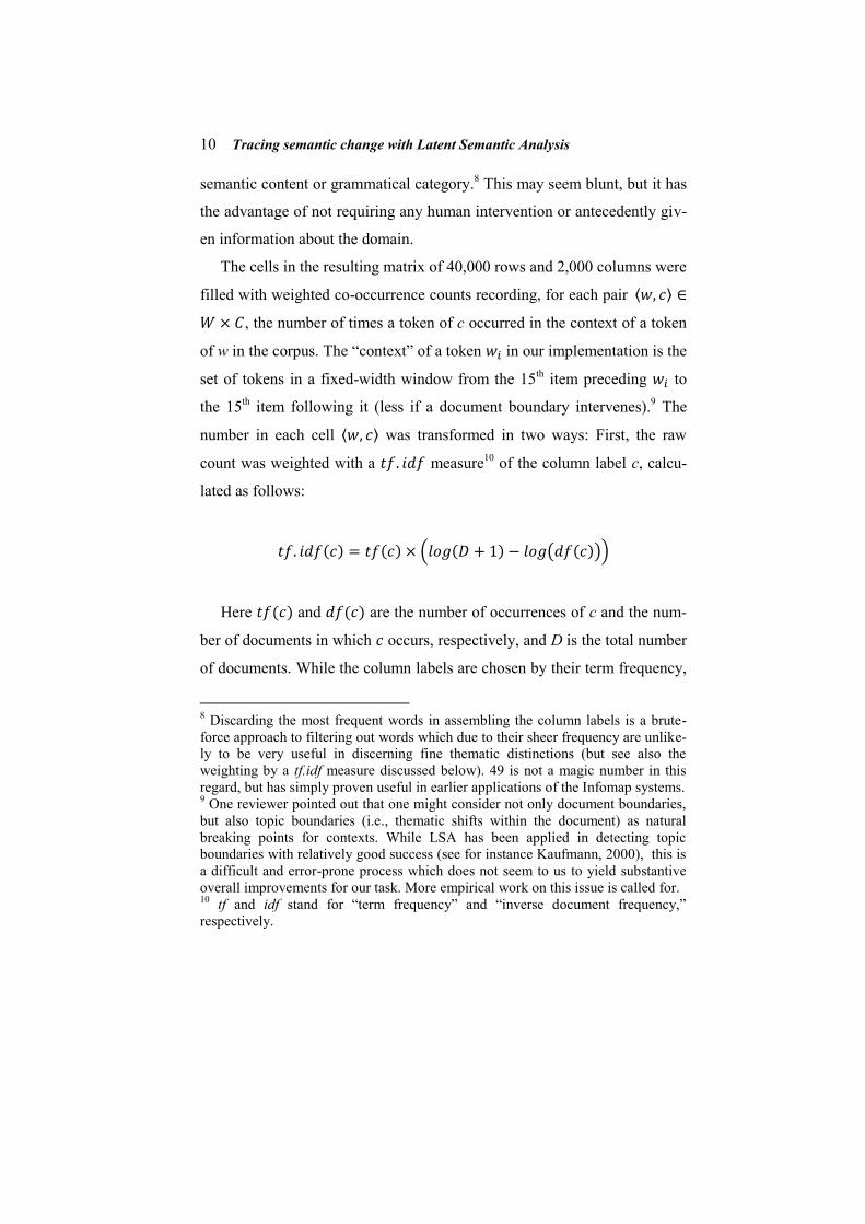
The cells in the resulting matrix of 40,000 rows and 2,000 columns were
filled with weighted co-occurrence counts recording, for each pair
, the number of times a token of c occurred in the context of a token
of w in the corpus. The “context” of a token in our implementation is the
set of tokens in a fixed-width window from the 15th item preceding to
the 15th item following it (less if a document boundary intervenes).
9 The
number in each cell was transformed in two ways: First, the raw
count was weighted with a measure10
of the column label c, calcu-
lated as follows:
Here and are the number of occurrences of c and the num-
ber of documents in which occurs, respectively, and D is the total number
of documents. While the column labels are chosen by their term frequency,
8 Discarding the most frequent words in assembling the column labels is a brute-
force approach to filtering out words which due to their sheer frequency are unlike-
ly to be very useful in discerning fine thematic distinctions (but see also the
weighting by a tf.idf measure discussed below). 49 is not a magic number in this
regard, but has simply proven useful in earlier applications of the Infomap systems. 9 One reviewer pointed out that one might consider not only document boundaries,
but also topic boundaries (i.e., thematic shifts within the document) as natural
breaking points for contexts. While LSA has been applied in detecting topic
boundaries with relatively good success (see for instance Kaufmann, 2000), this is
a difficult and error-prone process which does not seem to us to yield substantive
overall improvements for our task. More empirical work on this issue is called for. 10
tf and idf stand for “term frequency” and “inverse document frequency,”
respectively.
11
the weighting by inverse document frequency is intended to scale down
those columns labeled by words that are widely dispersed over the corpus.
The idea is that words whose occurrences are spread over many documents
are less useful as indicators of semantic content.11
Second, the number in
each cell is replaced with its square root, in order to approximate a normal
distribution of counts and attenuate the potentially distorting influence of
high base frequencies (cf. Takayama, et al. 1998; Widdows, 2004).
The matrix was further transformed by Singular Value Decomposition
(SVD), a dimension-reduction technique yielding a new matrix which is
less sparse (i.e., has fewer cells with zero counts) and with the property
that, roughly speaking, the first n columns, for any , capture as
much of the information about word similarities from the original matrix as
can be preserved in the lower n-dimensional space (Golub and Van Loan,
1989). The SVD implementation in the Infomap system relies on the
SVDPACKC package (Berry, 1992; Berry et al., 1993). The output was a
reduced matrix. Thus ultimately each item is asso-
ciated with a 100-dimensional vector .
2.2 Context vectors
Once the vector space for word types is obtained from the corpus, new
vectors can be derived for any multi-word unit of text (e.g. paragraphs,
queries, or documents), regardless of whether it occurs in the original cor-
11
Thus for instance, in most corpora the word do or its inflectional forms occur in
all documents, making them poor indicators of semantic content. While this
property does disqualify do as a “content-bearing” column label, it does not of
course impede the study the use of do itself, based on truly content-bearing words
in the contexts of its occurrences. We are grateful to an anonymous reviewer for
asking about this case.
12 Tracing semantic change with Latent Semantic Analysis
pus or not, as the normalized sum of the vectors associated with the words
it contains.12
In this way, for each occurrence of a target word type un-
der investigation, we calculated a context vector from the 15 items preced-
ing and the 15 items following that occurrence.13
Context vectors were first used in Word Sense Discrimination by
Schütze (1998). Similarly to that application, we assume that the “second-
order” context vectors represent the aggregate meaning or topic of the seg-
ment they are associated with, and thus, following the reasoning behind
LSA, are indicative of the meaning with which the target word is being
used on that particular occurrence. Consequently, for each target word w of
interest, the context vectors associated with its occurrences constitute the
data points. The analysis is then a matter of grouping these data points ac-
cording to some criterion (e.g., the period in which the text was written)
and conducting an appropriate statistical test. In some cases it might also be
possible to use regression or apply a clustering analysis.
2.3 Semantic density analysis
Conducting statistical tests comparing groups of vectors is not trivial. For-
tunately, some questions can be answered based on the similarity of vectors
12
The sum of m vectors with n dimensions is a vector
The inner product or dot product of two n-dimensional
vectors is . The length of a vector w is .
13 Since only 40,000 of the word types in the corpus are associated with vectors,
not all items in the window surrounding the target contribute to the context vector.
If a word occurs more than once in the window, all of its occurrences contribute to
the context vector.
13
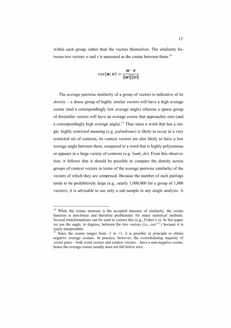
within each group, rather than the vectors themselves. The similarity be-
tween two vectors w and v is measured as the cosine between them:14
The average pairwise similarity of a group of vectors is indicative of its
density – a dense group of highly similar vectors will have a high average
cosine (and a correspondingly low average angle) whereas a sparse group
of dissimilar vectors will have an average cosine that approaches zero (and
a correspondingly high average angle).15
Thus since a word that has a sin-
gle, highly restricted meaning (e.g. palindrome) is likely to occur in a very
restricted set of contexts, its context vectors are also likely to have a low
average angle between them, compared to a word that is highly polysemous
or appears in a large variety of contexts (e.g. bank, do). From this observa-
tion, it follows that it should be possible to compare the density across
groups of context vectors in terms of the average pairwise similarity of the
vectors of which they are comprised. Because the number of such pairings
tends to be prohibitively large (e.g., nearly 1,000,000 for a group of 1,000
vectors), it is advisable to use only a sub-sample in any single analysis. A
14
While the cosine measure is the accepted measure of similarity, the cosine
function is non-linear and therefore problematic for many statistical methods.
Several transformations can be used to correct this (e.g., Fisher‟s z). In this paper
we use the angle, in degrees, between the two vectors (i.e., ) because it is
easily interpretable. 15
Since the cosine ranges from -1 to +1, it is possible in principle to obtain
negative average cosines. In practice, however, the overwhelming majority of
vector pairs – both word vectors and context vectors – have a non-negative cosine,
hence the average cosine usually does not fall below zero.

14 Tracing semantic change with Latent Semantic Analysis
Monte-Carlo analysis in which some number of pair-wise similarity values
is chosen at random from each group of vectors is therefore appropriate.16
However, there is one final complication to consider in the analysis. The
passage of time influences not only the meaning of words, but also styles
and varieties of writing. For example, texts in the 11th century were much
less varied, on average, than those written in the 15th century.
17 This will
influence the calculation of context vectors as those depend, in part, on the
text they are taken from. Because the document as a whole is represented
by a vector that is the average of all of its word vectors, it is possible to
predict that, if no other factors exist, two contexts are likely to be related to
one another to the same degree that their documents are. Controlling for
this effect can therefore be achieved by subtracting from the angle between
two context vectors the angle between the vectors of the documents in
which they appear.18
3 A diachronic investigation: Semantic change
3.1 Some background
Semantics is the study of the mapping between forms and meanings. Con-
sequently, the formal study of semantic change takes form-meaning pairs as
16
It is important to note that the number of independent samples in the analysis is
determined not by the number of similarity values compared but by the number of
individual vectors used in the analysis. 17
Tracking changes in the distribution of the document vectors in a corpus over
time might itself be of interest, but is beyond the scope of the current paper. 18
Subtraction of the angle between the document vectors was chosen because it
was the simplest and easiest method to implement. However, future work might
benefit from an approach that more fully explores the differences between the
documents within which the contexts are found and controls for them.
15
its object and explores changes in the association between the two. One
way to approach this task is to consider a fixed form F throughout various
periods in the history of the language and ask about the result-
ing sequence of form-meaning pairs, what
changes the meaning underwent. For instance, the expression as long as
underwent the change „equal in length‟ > „equal in time‟ > „provided that‟.
This is the kind of change we explore in our study. Another approach
would be to hold the meaning constant and look for changes in the forms
that express it (see Traugott, 1999 for discussion).
In this work we examine two of the traditionally recognized categories
of semantic change (Traugott, 2005:2-4; Campbell, 2004:254-262; Forston,
2003:648-650):
Broadening (generalization, extension, borrowing): A restricted
meaning becomes less restricted (e.g. Late Old English docga „a
(specific) powerful breed of dog‟ > dog „any member of the
species Canis familiaris‟
Narrowing (specialization, restriction): A relatively general
meaning becomes more specific (e.g. Old English deor „animal‟
> deer „deer‟)
Semantic change is generally the result of the use of language in varying
contexts, both linguistic and extralinguistic. Furthermore, the subsequent
meanings of a form are related to its earlier ones. As a result, the first sign
of semantic change is often the coexistence of the old and new meanings
(i.e., polysemy). Sometimes the new meanings become dissociated from the
earlier ones over time, resulting in homonymy (e.g., mistress „woman in a
16 Tracing semantic change with Latent Semantic Analysis
position of authority, head of household‟ > „woman in a continuing extra-
marital relationship with a man‟).
3.2 Hypotheses
As noted above, the main assumption underlying this project is that
changes in the meaning of a given word will be evident when examining
the contexts of its occurrences over time. For example, semantic broaden-
ing results in a meaning that is less restricted and as a result can be used in
a larger variety of contexts. In a semantic space that spans the period during
which the change occurred, the word‟s increase in versatility can be meas-
ured as a decrease in the density of its tokens, i.e., higher average angles
between the context vectors of the occurrences, across the time span of the
corpus. For instance, because the Old English word docga applied to a spe-
cific breed of dog, we predict that earlier occurrences of the lexemes docga
and dog, in a corpus of documents of the appropriate time period, will show
less variety and therefore higher density than later occurrences.19
The process of grammaticalization (Traugot and Dasher, 2002), in
which a content word becomes a function word, provides an even more
extreme case of semantic broadening. Since the distributions of function
words generally depend much less on the topic of the text than those of
content words, a word that underwent grammaticalization should appear in
a substantially larger variety of contexts than it did prior to becoming a
19
It is important to recall that because we measure variability of context compared
to the variability of the documents in question, the differences in the variability of
the documents between Middle English and Early Modern English is controlled for
and should not influence the analysis.
17
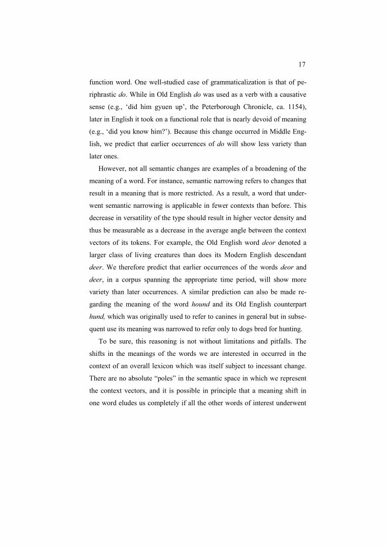
function word. One well-studied case of grammaticalization is that of pe-
riphrastic do. While in Old English do was used as a verb with a causative
sense (e.g., „did him gyuen up‟, the Peterborough Chronicle, ca. 1154),
later in English it took on a functional role that is nearly devoid of meaning
(e.g., „did you know him?‟). Because this change occurred in Middle Eng-
lish, we predict that earlier occurrences of do will show less variety than
later ones.
However, not all semantic changes are examples of a broadening of the
meaning of a word. For instance, semantic narrowing refers to changes that
result in a meaning that is more restricted. As a result, a word that under-
went semantic narrowing is applicable in fewer contexts than before. This
decrease in versatility of the type should result in higher vector density and
thus be measurable as a decrease in the average angle between the context
vectors of its tokens. For example, the Old English word deor denoted a
larger class of living creatures than does its Modern English descendant
deer. We therefore predict that earlier occurrences of the words deor and
deer, in a corpus spanning the appropriate time period, will show more
variety than later occurrences. A similar prediction can also be made re-
garding the meaning of the word hound and its Old English counterpart
hund, which was originally used to refer to canines in general but in subse-
quent use its meaning was narrowed to refer only to dogs bred for hunting.
To be sure, this reasoning is not without limitations and pitfalls. The
shifts in the meanings of the words we are interested in occurred in the
context of an overall lexicon which was itself subject to incessant change.
There are no absolute “poles” in the semantic space in which we represent
the context vectors, and it is possible in principle that a meaning shift in
one word eludes us completely if all the other words of interest underwent
18 Tracing semantic change with Latent Semantic Analysis
just the right kind of shift themselves. This risk is of course not limited to
computational methods, but faced by human investigators as well. We be-
lieve that it could be minimized by tracking changes on a “global” scale,
looking for patterns in the vocabulary as a whole. Computational methods
like ours are in principle well-suited to this task, which is why we men-
tioned this application as one of their potential advantages. Implementing
and testing our method on such a large scale is not trivial, however, and
beyond the scope of the present study. Meanwhile, we believe that such a
case of simultaneous shifts is highly unlikely, and our results suggest that
the method can be used fruitfully despite this caveat.
3.3 Materials
We used a corpus derived from the Helsinki corpus (Rissanen, 1994) to
test these predictions. The Helsinki corpus is comprised of texts spanning
the periods of Old English (prior to 1150A.D.), Middle English (1150-
1500A.D.), and Early Modern English (1500-1710A.D.). Because spelling
in Old English was highly variable, we decided to exclude that part of the
corpus and focused our analysis on the Middle English and Early Modern
English periods.20
The resulting corpus included 504 distinct documents
totaling approximately 1.15 million words (approximately 200,000 from
early Middle English texts, 400,000 from late Middle English texts, and
550,000 from Early Modern English texts).
20
While the spelling in Middle English, especially during the earlier periods, is
also quite variable, it is still less variable than that found in Old English. Because
semantic change takes time, we expect to see at least part of these shifts in Middle
English and Early Modern English.
19
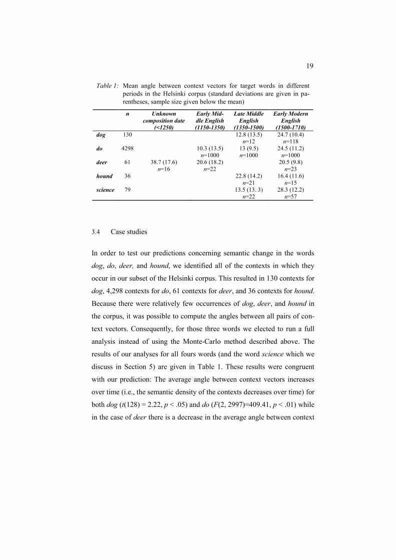
3.4 Case studies
In order to test our predictions concerning semantic change in the words
dog, do, deer, and hound, we identified all of the contexts in which they
occur in our subset of the Helsinki corpus. This resulted in 130 contexts for
dog, 4,298 contexts for do, 61 contexts for deer, and 36 contexts for hound.
Because there were relatively few occurrences of dog, deer, and hound in
the corpus, it was possible to compute the angles between all pairs of con-
text vectors. Consequently, for those three words we elected to run a full
analysis instead of using the Monte-Carlo method described above. The
results of our analyses for all fours words (and the word science which we
discuss in Section 5) are given in Table 1. These results were congruent
with our prediction: The average angle between context vectors increases
over time (i.e., the semantic density of the contexts decreases over time) for
both dog (t(128) = 2.22, p < .05) and do (F(2, 2997)=409.41, p < .01) while
in the case of deer there is a decrease in the average angle between context
Table 1: Mean angle between context vectors for target words in different
periods in the Helsinki corpus (standard deviations are given in pa-
rentheses, sample size given below the mean)
n Unknown
composition date
(<1250)
Early Mid-
dle English
(1150-1350)
Late Middle
English
(1350-1500)
Early Modern
English
(1500-1710)
dog 130 12.8 (13.5)
n=12
24.7 (10.4)
n=118
do 4298 10.3 (13.5)
n=1000
13 (9.5)
n=1000
24.5 (11.2)
n=1000
deer 61 38.7 (17.6)
n=16
20.6 (18.2)
n=22
20.5 (9.8)
n=23
hound 36 22.8 (14.2)
n=21
16.4 (11.6)
n=15
science 79 13.5 (13. 3)
n=22
28.3 (12.2)
n=57
20 Tracing semantic change with Latent Semantic Analysis
vectors, indicating an increase in the semantic density of the contexts over
time (F(2, 58) = 8.82, p < .01). However, while the semantic density of the
contexts of hound appears to increase over time, this trend is not statistical-
ly significant (t(34) = -1.50, n.s.). It is likely that this last difference was
not statistically significant due to a lack of statistical power. Because our
method relies on statistics rather than human intuition and reasoning, it is to
be expected that it requires a larger corpus in order to be effective.
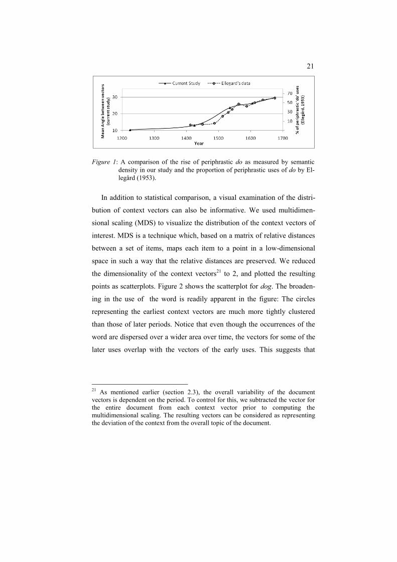
To supplement the above analysis, we compared our observations on do
with the data collected by Ellegård (1953). Ellegård mapped out the gram-
maticalization of do through a manual examination of the changes in the
proportions of its various uses between 1400 and 1700. He identified an
overall shift in the pattern of use that occurred mainly between 1475 and
1575. Our statistical analysis shows a comparable shift in patterns between
the time periods spanning 1350-1500 and 1500-1570. Figure 1 depicts an
overlay of both datasets. The relative scale of the two sets was set so that
the proportions of do uses at 1400 and 1700 (the beginning and end of El-
legård‟s data, respectively) match the semantic density measured by our
method at those times. We see that not only the direction, but also the rate
of the change as detected by these respective methods are quite similar.
21
In addition to statistical comparison, a visual examination of the distri-
bution of context vectors can also be informative. We used multidimen-
sional scaling (MDS) to visualize the distribution of the context vectors of
interest. MDS is a technique which, based on a matrix of relative distances
between a set of items, maps each item to a point in a low-dimensional
space in such a way that the relative distances are preserved. We reduced
the dimensionality of the context vectors21
to 2, and plotted the resulting
points as scatterplots. Figure 2 shows the scatterplot for dog. The broaden-
ing in the use of the word is readily apparent in the figure: The circles
representing the earliest context vectors are much more tightly clustered
than those of later periods. Notice that even though the occurrences of the
word are dispersed over a wider area over time, the vectors for some of the
later uses overlap with the vectors of the early uses. This suggests that
21
As mentioned earlier (section 2.3), the overall variability of the document
vectors is dependent on the period. To control for this, we subtracted the vector for
the entire document from each context vector prior to computing the
multidimensional scaling. The resulting vectors can be considered as representing
the deviation of the context from the overall topic of the document.
Figure 1: A comparison of the rise of periphrastic do as measured by semantic
density in our study and the proportion of periphrastic uses of do by El-
legård (1953).

22 Tracing semantic change with Latent Semantic Analysis
while the meaning of dog broadened, the word did not lose its original
meaning altogether.
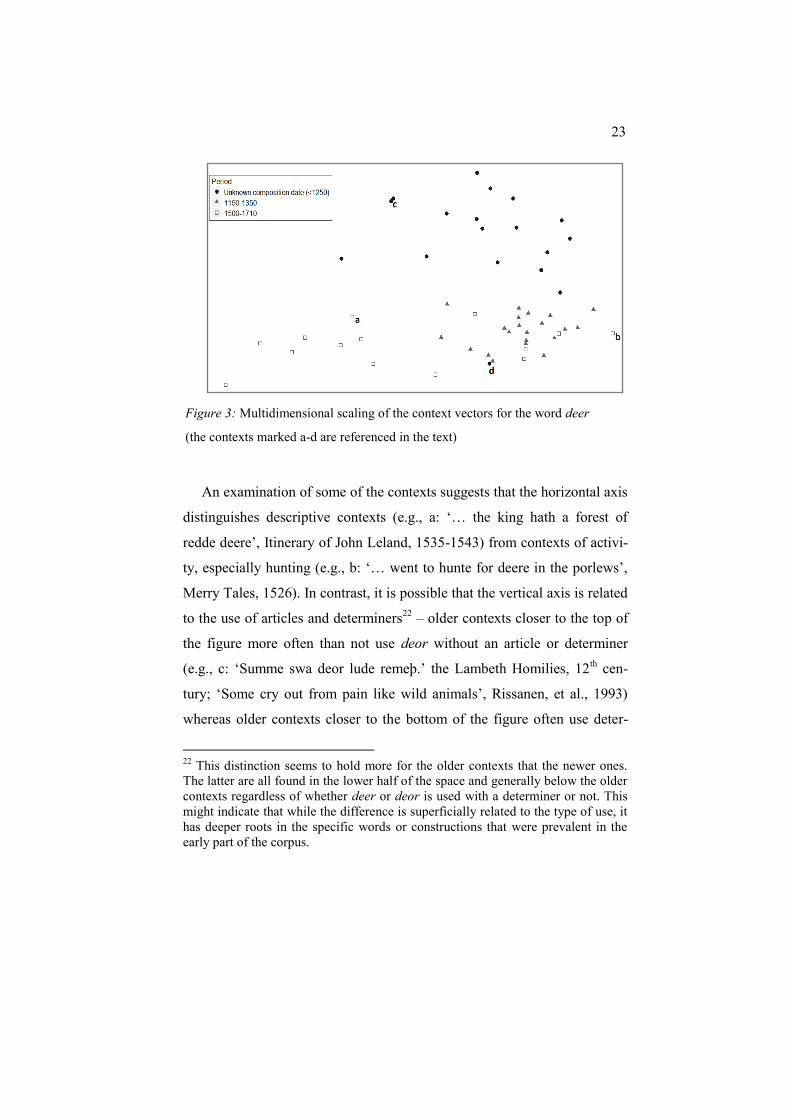
Similarly, the narrowing in the meaning of deer is evident when ex-
amining the scatterplot of its context vectors (Figure 3). The circles
representing the contexts of the earliest occurrences are spread out more
than those in later periods. However, unlike in the case of dog, the vectors
from the early period seem to generally occupy a different part of the MDS
space than those of later periods. This suggests that in addition to the nar-
rowing that is evident from the increasing density of the vectors, there was
also a more fundamental shift in how deer was used. Specifically, some of
the ways in which it was used in Old and early Middle English may no
longer be prevalent in Early Modern English.
Period
1150-1350
1350-1500
1500-1710
Figure 2: Multidimensional scaling of the context vectors for the word dog
23
An examination of some of the contexts suggests that the horizontal axis
distinguishes descriptive contexts (e.g., a: „… the king hath a forest of
redde deere‟, Itinerary of John Leland, 1535-1543) from contexts of activi-
ty, especially hunting (e.g., b: „… went to hunte for deere in the porlews‟,
Merry Tales, 1526). In contrast, it is possible that the vertical axis is related
to the use of articles and determiners22
– older contexts closer to the top of
the figure more often than not use deor without an article or determiner
(e.g., c: „Summe swa deor lude remeþ.‟ the Lambeth Homilies, 12th cen-
tury; „Some cry out from pain like wild animals‟, Rissanen, et al., 1993)
whereas older contexts closer to the bottom of the figure often use deter-
22
This distinction seems to hold more for the older contexts that the newer ones.
The latter are all found in the lower half of the space and generally below the older
contexts regardless of whether deer or deor is used with a determiner or not. This
might indicate that while the difference is superficially related to the type of use, it
has deeper roots in the specific words or constructions that were prevalent in the
early part of the corpus.
Figure 3: Multidimensional scaling of the context vectors for the word deer
(the contexts marked a-d are referenced in the text)

24 Tracing semantic change with Latent Semantic Analysis
miners such as the (e.g., d:„Alle þa deor and alle ϸe nutenu þe on eorðe
weren.‟, the Lambeth Homilies, 12th century; „All the wild animals and all
the domestic animals which were on earth‟). Importantly, this analysis is
focused on exploring the shifts observed in Figure 3. While the interpreta-
tion of the horizontal axis could potentially provide some interesting in-
sights regarding the nature of the shift in meaning of deer beyond its well
documented narrowing, the inferred interpretation of the vertical axis simp-
ly reiterates a well known observation – namely that the use of determiners
increases over time.
4 Discussion
The method we presented in this paper attempts to statistically analyze
semantic relationships that were previously difficult to quantify. However,
this use raises an interesting theoretical question regarding the relationship
between the statistically computed semantic space and the actual semantic
content of words. While simulations based on Latent Semantic Analysis
have been shown to correlate with cognitive factors such as the categoriza-
tion of texts and the acquisition of vocabulary (cf. Landauer & Dumais,
1997), in reality speakers‟ use of language relies on more than mere pat-
terns of word co-occurrence. For example, syntactic structures and prag-
matic reasoning are used extensively to supplement the meaning of the
individual lexemes we come across (e.g., Fodor, 1995; Grice, 1989 [1975]).
Moreover, the very nature of the word co-occurrence patterns used in
Latent Semantic Analysis limits the type of semantic information it can
uncover. One such well known limitation regards negation of meaning and
antonyms. Both of these result in a meaning that is the opposite of the orig-

25
inal (e.g., happy vs. not happy or sad). However, because a word and its
antonyms appear in similar contexts, methods that rely on word co-
occurrence patterns would judge that their meaning is similar. Likewise,
because negation is realized through the use of function words rather than
content-bearing words, such meanings cannot easily be captured by me-
thods such as Latent Semantic analysis.
It is therefore likely that while LSA captures some of the variability in
meaning exhibited by words in context, it does not capture all of it. Indeed,
there is a growing body of methods that propose to integrate statistical me-
thods such as LSA with methods that rely on a structured analysis of lan-
guage such as syntactic analysis and formal semantics (e.g., Pado and La-
pata, 2007; Widdows, 2003, Wiemer-Hastings, 2000).
That said, it appears that enough of the semantic content of word mean-
ing is captured by LSA for semantic density to be a useful measure of the
broadness of word meaning. Specifically, we observed sufficient changes in
the semantic density of word meaning over time to identify patterns of both
semantic broadening and semantic narrowing in a couple of cases with a
relatively small sample size (e.g., dog and deer). To be sure, for statistical
methods it is preferably to have a larger sample size whenever possible.23
Regardless of any such limitations, in this paper we demonstrated that
important information about meaning can be gathered through a systematic
analysis of the contexts in which words appear and the changes these con-
texts undergo over time. Furthermore, we believe that the role of context in
23
It remains to be seen whether this method can distinguish between other kinds of
semantic change, such as pejoration and amerlioration as they require a fine-
grained distinction between “positive” and “negative” meanings. The growing field
of sentiment analysis in the computational literature may provide useful tools for
this application.
26 Tracing semantic change with Latent Semantic Analysis
semantic change is likely to be an active one. For example, when we come
across a word we are unfamiliar with, the context in which we encounter it
can often give us some clues as to its meaning. Likewise, if we come across
a familiar word in a context in which it does not seem to fit well, this unex-
pected encounter may induce us to adjust our representation of both the
context and the word so that the utterance or sentence becomes more cohe-
rent. The importance of the contexts in which a word appears for its mean-
ing and more specifically for changes to its meaning over time suggests a
dynamic view of semantics as an ever-changing landscape of meaning. In
such a view, semantic change is the norm, as the perceived meanings of
words keep shifting to accommodate the contexts in which they are used.
5 Future work: Discovery
Finally, at least in some cases our method can be used not only to test pre-
dictions based on established cases of semantic change, but also to identify
new ones. While there are several well known examples of semantic
change (e.g., deer, dog and hound), many other words have likely under-
gone change in meaning over the centuries. Researchers interested in such
cases can use the method described here to rapidly identify whether such a
change is likely for a specific word. For instance, we examined the word
science without any preexisting hypothesis as to possible semantic change
that it might have undergone, disregarding the discussions of its history in
the linguistic literature (e.g., Hughes, 2000). Our initial analysis of its con-
texts uncovered that it underwent semantic broadening shortly after it first
appeared in the 14th century (t(77) = 4.51, p < .01). A subsequent examina-
tion of the contexts in which the word appears indicated that this is proba-

27
bly the result of a shift from a meaning related to knowledge in a basic,
generic sense (e.g., „…and learn science of school‟, John of Trevisa‟s Po-
lychronicon, 1387) to one that can be used to refer to more specific discip-
lines of systematic inquiry in addition to its original use (e.g., „…of the
seven liberal sciences‟, Simon Forman‟s Diary, 1602). This shift involves a
mass-to-count change in the core meaning of the noun; in addition, its new
uses may have at least partly displaced earlier senses of art/arts. More work
is required to trace the exact time course of these changes in detail.
Our long-term goal is to use this method in a computer-based tool that
can scan a diachronic corpus and automatically identify probable cases of
semantic change within it. Researchers can then use these results to focus
on identifying the specifics of such changes, as well as examine the overall
patterns of change attested in the corpus. It is our belief that while no such
system is likely to supplant the researcher‟s intuition entirely, it will enable
a more rigorous testing and refinement of existing theories of semantic
change.
6 Acknowledgments
We would like to thank the audience at ICEHL for valuable feedback, as
well as two anonymous referees for detailed comments and the editors for
their patience and support. The second author thanks the American Council
of Learned Societies (ACLS) and the Lichtenberg-Kolleg at Georg-August-
Universität Göttingen for support during part of this project.
28 Tracing semantic change with Latent Semantic Analysis
7 References
Berry, M. W.
1992 SVDPACK: A Fortran-77 Software Library for Sparse Singular
Value Decomposition. Tech. Rep. CS-92-159, Knoxville, TN: Uni-
versity of Tennessee.
1992 Large scale singular value computations. International Journal of
Supercomputer Applications 6:13-49.
Berry, M. W., T. Do, G. O‟Brien, K. Vijay, and S. Varadhan
1993 SVDPACKC (Version 1.0) User’s Guide, Tech. Rep. UT-CS-93-194.
Knoxville, TN: University of Tennessee.
Campbell, L.
2004 Historical Linguistics: An Introduction, 2nd
ed. Cambridge, MA: The
MIT Press.
Dam, G. and Kaufmann, S.
2008 Computer assessment of interview data using Latent Semantic Anal-
ysis. Behavior Research Methods 40:8-20.
Deerwester, S., S. T. Dumais, G. W. Furnas, T. K. Landauer, and R. Harshman
1990 Indexing by Latent Semantic Analysis. Journal of the American
Society for Information Science 41:391-407.
Ellegård, A.
1953 The auxiliary do: The establishment and regulation of its use in Eng-
lish. Gothenburg Studies in English, 2. Stockholm: Almqvist and
Wiksell.
Firth, J.
1930 Speech. London: Benn's sixpenny library.
1957 Papers in Linguistics, 1934-1951. London: Oxford University Press.
Fodor, J. D.
29
1995 Comprehending sentence structure. In Invitation to Cognitive
Science, volume 1, Gleitman, L. R. and M. Liberman, (eds.), 209-
246. Cambridge, MA: The MIT Press.
Forston, B. W.
2003 An approach to semantic change. In The Handbook of Historical
Linguistics, Joseph, B. D., and R. D. Janda (eds.), 648-666. Malden,
MA: Blackwell Publishing.
Grice, H. P.
1989 Logic and Conversation. In Studies in the Way of Words, 22-40.
Cambridge, MA: Harvard University Press.
Golub, G. H., and C. F. Van Loan
1989 Matrix Computations, 2nd
edition. Balitimore, MD: The Johns
Hopkins University Press.
Graesser, A. C., K. Wiemer-Hastings, P. Wiemer-Hastings, R. Kreuz and Tutorial
Research Group
1999 AutoTutor: A simulation of a human tutor. Journal of Cognitive
Systems Research 1:35-51
Halliday, M. A. K., and R. Hasan
1976 Cohesion in English. London: Longman.
Hock, H. H., and B. D. Joseph
1996 Language History, Language Change, and Language Relationship:
An Introduction to Historical and Comparative Linguistics. Berlin:
Mouton de Gruyter.
Hoey, M.
1991 Patterns of Lexis in Text. London: Oxford University Press.
Hughes, G.
2000 A History of English Words. Malden, MA: Blackwell.
Infomap [Computer Software]
2007 http://infomap-nlp.sourceforge.net/ Stanford, CA.
Kaufmann, S.
30 Tracing semantic change with Latent Semantic Analysis
2000 Second-order cohesion. Computational Intelligence 16:511-524.
Landauer, T. K., and S. T. Dumais
1997 A solution to Plato‟s problem: The Latent Semantic Analysis theory
of the acquisition, induction, and representation of knowledge. Psy-
chological Review 104:211-240.
Landauer, T. K., D. S. McNamara, S. Dennis, and W. Kintsch
2007 Handbook of Latent Semantic Analysis. Mahwah, NJ: Lawrence
Erlbaum Associates.
Levin, E., M. Sharifi, and J. Ball
2006 Evaluation of utility of LSA for word sense discrimination. In Pro-
ceedings of the Human Language Technology Conference of the
NAACL, Companion Volume: Short Papers, 77-80. New York City.
Manning, C. D., P. Raghavan, and H. Schütze
2008 Introduction to Information Retrieval. New York: Cambridge Uni-
versity Press.
Manning, C. D., and H. Schütze
1999 Foundations of Statistical Natural Language Processing. Cam-
bridge, MA: The MIT Press.
Marcu, D.
2003 Automatic Abstracting. In Encyclopedia of Library and Information
Science, Drake, M. A. (ed.), 245-256. New York : Marcel Dekker.
Otis, K. and E. Sagi
2008 Phonaesthemes: A Corpora-based Analysis. In Proceedings of the
30th Annual Conference of the Cognitive Science Society, Love B.
C., K. McRae, & V. M. Sloutsky (eds.), 65-70. Austin, TX: Cogni-
tive Science Society.
Pado, S. and M. Lapata
2007 Dependency-based construction of semantic space models. Compu-
tational Linguistics 33:161-199.
Riedel E., S. L. Dexter, C. Scharber, and A. Doering
31
2006 Experimental evidence on the effectiveness of automated essay scor-
ing in teacher education cases. Journal of Educational Computing
Research 35:267-287.
Rissanen, M.
1994 The Helsinki Corpus of English Texts. In Corpora Across the Centu-
ries: Proceedings of the First International Colloquium on English
Diachronic Corpora, Kytö, M., M. Rissanen, and S. Wright (eds).
Amsterdam: Rodopi.
Rissanen, M., M. Kytö, and M. Palander-Collin
1993 Early English in the computer age: explorations through the Helsin-
ki corpus. Berlin: Mouton de Gruyter
Schütze, H.
1996 Ambiguity in Language Learning: Computational and Cognitive
Models. Stanford, CA: CSLI Publications.
1998 Automatic word sense discrimination. Computational Linguistics
24:97-124.
Steinhart, D. J.
2001 Summary Street: An Intelligent Tutoring System for Improving Stu-
dent Writing through the Use of Latent Semantic Analysis. PhD The-
sis, University of Colorado, Boulder.
Takayama, Y., R. Flournoy, and S. Kaufmann
1998 Information Mapping: Concept-Based Information Retrieval Based
on Word Associations. Stanford, CA: CSLI Publications.
Takayama, Y., R. Flournoy, S. Kaufmann, and S. Peters
1999 Information retrieval based on domain-specific word associations. In
Proceedings of the Pacific Association for Computational Linguis-
tics (PACLING’99), Cercone, N. and K. Naruedomkul (eds.), 155-
161. Waterloo, Canada.
Traugott, E. C.
32 Tracing semantic change with Latent Semantic Analysis
1999 The role of pragmatics in semantic change. In J. Verschueren (ed.),
Pragmatics in 1998: Selected Papers from the 6th International
Pragmatics Conference, vol. II., 93-102. Antwerp: International
Pragmatics Association.
2005 Semantic change. In Encyclopedia of Language and Linguistics, 2nd
ed., Brown K. (ed.). Oxford: Elsevier.
Traugott, E. C., and R. B. Dasher
2002 Regularity in Semantic Change. New York: Cambridge University
Press.
Widdows, D.
2003 Unsupervised methods for developing taxonomies by combining
syntactic and statistical information. In Proceedings of the joint Hu-
man Language Technology Conference and Annual Meeting of the
North American Chapter of the Association for Computational Lin-
guistics, 197-204. Edmonton, Canada: Wiemer-Hastings.
2004 Geometry and Meaning. Stanford, CA: CSLI Publications.
Wiemer-Hastings, P.
2000 Adding syntactic information to LSA. In Proceedings of the Twenty-
Second Annual Conference of the Cognitive Science Society, Gleit-
man, L. A. and A. K. Joshi (eds.), 989-993. Mahwah, NJ: Erlbaum.
Wiemer-Hastings, P., K. Wiemer-Hastings, and A. C. Graesser
1999 Improving an intelligent tutor‟s comprehension of students with
Latent Semantic Analysis, in Artifical Intelligense in Education, Le
Mans, France, 535-542. Amsterdam: IOS Press.