TR/11 July 1972

SARD KERNEL THEOREMS ON TRIANGULAR

AND RECTANGULAR DOMAINS WITH

EXTENSIONS AND APPLICATIONS TO

FINITE ELEMENT ERROR BOUNDS by

R. E. Barnhill and J. A. Gregory.

The research of R. E. Barnhill was supported by The National Science Foundation with Grant GP 20293 to the University of Utah, by the Science Research Council with Grant B/SR/9652 at Brunel University, and by a N.A.T.O. Senior Fellowship in Science.

1.

1. Introduction

The purpose of this paper Is to derive error bounds for

the finite element analysis of elliptic boundary value problems.

As shown in Section 2, the interpolation remainder is an upper

bound on the finite element remainder in the appropriate norm.

Error bounds are derived for the interpolation remainder by

means of extensions of the Sard kernel theorems. The Sard kernel

theorems provide a representation of admissible linear functionals

on spaces of functions with a prescribed smoothness. If appropriate

derivatives of the solution u of the boundary value problem can

be found, then these theorems yield computable error bounds.

These theorems have been applied to cubatures by Stroud [10] and

by Barnhill and Pilcher [1].

The solutions of elliptic boundary value problems are usually

assumed to be in a Sobolev space. The Sobolev and Sard spaces

are not the same. If (a,b) is the point about which Taylor

expansions are taken in the Sard space, then the Sobolev spaces

are contained in the Sard spaces of the same order for almost

all a and for almost all b. In Section 3, we show that the

derivatives occurring in the Sard spaces can be generalized

derivatives, so that the derivatives in the two types of spaces

are of the same kind.

Some of the functionals of finite element interest are not,

in general, admissible for Sard spaces. A precise statement of

this is given in Section 2. This problem was avoided by Birkhoff,

Schultz and Varga [4] in a way that is appropriate for rectangles,

but is inappropriate for triangles because it implies the use of

derivatives outside the original region of interest. In Section 4,

2.

2.

we extend the kernel theorems and show how to choose the

point (a,b) so that the finite element functionals can be applied

in an arbitrary triangle. The method can also be used for more

general regions.

The finite element functionals do not involve all possible

derivatives of a certain order. In Section 5, we prove a Zero

Kernel Theorem that states sufficient conditions for certain of

the Sard kernels to be identically zero. The Zero Kernel Theorem

has various applications, one being that certain mesh restrictions

in Birkhoff, Schultz and Varga can be avoided.

We conclude in Section 6 with computed examples of the

constants in the error bound for piecewise linear and piecewise

quadratic interpolation.

The Galerkin Method and Its Relationship to Interpolation.

Finite element analysis means piecewise approximation over a

set of geometric "elements". This rather general definition

suffices e.g., for computer-aided geometric design, but for

elliptic boundary value problems finite element analysis usually

means the Galerkin method. If the partial differential equation

is the Euler equation for a variational problem, then the

Rayleigh-Ritz method is applicable and is the same as the

Galerkin method. Thus the Galerkin method is the more general

since it does not depend upon the existence of some underlying

variational problem. Therefore, we discuss only the Galerkin

method in this paper.

Let Ω be a simply connected bounded region that satisfies

a restricted cone condition in the xy- plane. For p > 1 and ℓ

a non-negative integer, is the Sobolev space of functions ( )ΩloW

3.

with all ℓth order generalized derivatives existing and in

L p (Ω). Usually p = 2 . We recall that for Ω as in Figure 1,

1,0uxu

=∂∂ is the (1,0) generalized derivative of u means that

u1,0 is in L1(Ω) and

∫∫∂∂

−∫∫ ∫⎥⎥⎦

⎤

⎢⎢⎣

⎡ ===

∂∂

Ω(2.1)dydx

xvudy

Ω

d

c

(y)2xx(y)1xxy)(x,vy)u(x,dydxv

xu

for all test functions v in )(12 Ωw

( )

∫∫−=∫∫

∈∂≡

Ωdydx1,0vudydxv

Ω ,01u

Ω12

0WVi.eΩon0V then

(2.2)

:followingtheis)(Ω2wfornormA l

( ) ∂≤

∑=∂

|α |21

2)2L| |vαD | (|Ω2 W| | v| | (2.3)

α2yα1x

ααD,)2α,1(ααwhere∂∂

∂==

and the summation in (2.3) is over all α such that

|α| = α1 + α2 ≤ ℓ. The definition of generalized derivative

4. implies that the partials in can be taken in any order. αD

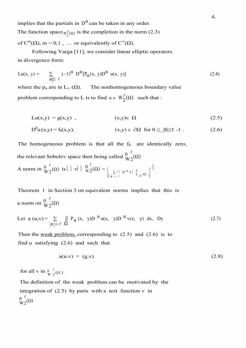
The function space is the completion in the norm (2.3) ( )Ω2W∂

of Cm(Ω), m = 0,1 , ... or equivalently of C∞(Ω).

Following Varga [11], we consider linear elliptic operators

in divergence form:

(2.4)y)]u(x,α

αy)D(x,α[PαDα1)(y)Lu(x, ∑≤

−=l

where the pα are in L∞ (Ω). The nonhomogeneous boundary value

problem corresponding to L is to find such that : ( )Ω2Wu l∈

Lu(x,y) = g(x,y) , (x,y)∈ Ω (2.5)

Dßu (x,y) = fß(x,y), (x,y) ∈ ∂Ω for 0 ≤_|ß|≤ℓ -1 . (2.6)

The homogeneous problem is that all the fß are identically zero,

the relevant Sobolev space then being called ( )Ω20Wl

A norm in is v = ( )Ω20Wl

( )Ω20wl

.21

2Ω2Lv

α

αD⎪⎭

⎪⎬⎫

⎪⎩

⎪⎨⎧

∑=

⎟⎠⎞⎜

⎝⎛

l

Theorem 1 in Section 3 on equivalent norms implies that this is

a norm on ( )Ω20Wl

Let a (u,v) = (2.7)Dydx,y)v(x,αy)Du(x,

ααy)D(x,

ΩαP∑

=∫∫

l

Then the weak problem, corresponding to (2.5) and (2.6) is to

find u satisfying (2.6) and such that

a(u.v) = (g,v) (2.8) for all v in ( )Ω2

0W

l

The definition of the weak problem can be motivated by the

integration of (2.5) by parts with a test function v in

( )Ω20Wl

5.

We consider interpolants u to u, where the interpolation ~

conditions are the following:

(2.9),n....,,1j,(u)jM)~u(jM

,m....,,1i,(u)iL)~u(iL

====

and the Li and Mj. are interpolation functionals such that

the Li(u) are unknown and the Mj.(u) are known a priori.

Hereafter we assume that the Mj(u) are known from the

boundary data (2.6). −Ω is usually discretized and the linear funotionals Li and

Mj based on the discretization, an example being the

evaluation of u and its derivatives at certain mesh points.

Let vh be an (m + n)-dimensional subspace of such )(Ω2wl

that the L.i and Mj are linearly independent over vh. Then Vh has a

basis of functions n1jy)(x,jcandm

1iy)(x,iB == that

are biorthonormal with respect to the Li and Mj [5]. Let

Sh be the subset of which consists of functions v of )(Ω2wl

the form

y)(x,jc

n

1j(u)iMy)(x,iB

m

1i ia y)v(x, ∑=

+∑=

=

where the ai are constants. Let be the m-dimensional h0s

subspace generated by the Bi. The Galerkin method is to

find U in Sh such that a(U,v) = (g,v) for all v in . (2.10) h0s

The"conforming condition" is that ,which is )(Ω2whs l⊂

required for the Galerkin method. We also require

,)(Ω20wh

0sl

⊂ which usually follows from the conforming condition.

Lemma.1 (Strang [9]). The Galerkin approximation U is the best

approximation from Sh to u in the energy norm induced by

6.

the inner product a(u,v). That is,

a(u -U, u - U) ≤ a(u - u~ , u - u~ for all u~ in Sh (2.11)

In fact,

.)~u,~u(a)U~U,~(aU)u,U(ua uuuu −−=−−+−− (2.12)

Proof: From the definitions of weak problem (2.3) and

Galerkin method, (2.10), a(u - U,v) = 0 for all v in .h0s

Therefore, a( u - U, u - U) = =−−−− U),Uu~(aand,)u~uU,(ua

,)Uu(u,ua( −− ~~ from which (2.12) follows. Q.E.D.

The normal equations for this beat approximation can be

derived as follows:

If u~ interpolates to u with respect to the functionals

Li and Mj, then

)y(x,jc(u)n

1j jMy)(x,iBiAy)U(x,Hence

)y(x,jc(u)n

1j jMy)(x,i(u)Bm

11i iL)y,x(u

∑=

+∑=

∑=

+∑=

= 3) (2.~

and a(U,Bk ) = (g,Bk) k =- 1, ...., m.

m.,....,1k

,)kB,n

1j ja(c(u)jM)kB(g,)kB,ia(Bm

1i iA

Thus

=

∑=

−=∑=

(2.14) Equations (2.14) yield a method of calculation of the Ai.

Since the Bk are in the actual normal equations are ,)(Ω20wl

7. the following :

(2.15)m.1,.....,k),kB,j(u)Cn

1j jMa(u)kB,ia(Bm

1i iA =∑=

−=∑=

The norm induced by a(u,v) is equivalent to the

norm if a is bounded and - elliptic, i.e. )(Ω2wl )(Ω2w l

Elliptic : ( )

0ρconstantsomeand(2.16)Ω2Wvεallforv)a(v,2

Ω2W||v||ρ

>≤

⎟⎠⎞⎜

⎝⎛

ll

( ) (2.17)Ω2Wεwv,allfor2W

||w||2W

||v|| ||a||w)a(v,:|Bounded lll≤

( ) (2.17)ΩL||Pα||max|α|||a||(2.4),From ∞≤≤l

Lemma 2. Assumptions (2.16),(2.17) imply that

(2.18)2W||u-u||minhεSu

21

ρ||a||

2W||U-u|| ll ~~⎭

⎬⎫

⎩⎨⎧

≤

Proof : The best approximation property a (u-U,u-U) < a ),uu,u(u ~~ −−

ellipticity ,and boundedness imply the conclusion . Q.E.D.

Example. For Poisson's equation, ℓ = 1, | |a| |= 1 and ρ

can be taken as one.

Interpolation remainder theory is applicable to the Galerkin

method from the best approximation property (2.11) or

equivalently, from (2.18), the interpolant being taken as u~

3. The Sobolev Imbedding Theorems.

The following theorem on equivalent norma [7] was used in

Section 2:

Theorem 1. If F1,.. .FN are bounded linear functionals on

that are linearly independent over P)(Ω2wl

ℓ-1 , the space of

polynomials of degree ≤ ℓ - 1 , and N = ℓ(ℓ+l)/2, then the usual

8.

21

|α|)(Ω2

2L||vαD||2|(v)N

1k kF|||v||

normthebyreplacedbecan(2.3)norm)(Ω2w

⎪⎭

⎪⎬⎫

⎪⎩

⎪⎨⎧

∑=

+∑=

=+l

l

(3.1)

The norm on is obtained with the F( )Ω20W

lk being

of the form ∫∂

−−<Ω

1β,dsuβD l

The Fk are bounded because lower order derivatives can be

bounded in terms of higher order derivatives as follows:

Theorem 2. Let Ω be the union of finitely many star-like

regions. If ℓ = 1 , then v in implies that )(Ω12w

( ) ||1ΩL2|| v|| ≤ ℒ ( ) ( ) ( ) (3.2)Ω12W

||v||1Ω2LΩ12W

|| →

where Ω1 is a one-dimensional subset of −Ω .

If ℓ > 1 , then v in implies that )(Ω2wl

||ℒ||( ) ≤Ω2-C||v|| l ( ) ( ) ( ) (3.3)Ω2W||v||1Ω2LΩ2W ll →

Where ||ℒ|| x→y means the norm of the operator imbedding

X into Y.

We note from Theorem 2 that point evaluation funotionals are

bounded on W (Ω). However, these functionals are unbounded 22

on w 12 (Ω).

A specific example of Theorem 2 is the following:

Lemma 3. Let Ω be a bounded convex region with B equal to

the maximum of Bx and By , where Bx is the diameter of Ω along

parallels to the x-axis and By is dual.

If u ≡ 0 on ∂Ω, then

( ) ( ) (3.4)Ω12

0W||u||B

2Ω2L||u|| ≤

9.

Proof: Let ∂Ω be parametrized by the pair of functions

y1 (x) ≤ y2 (x), a ≤ x ≤ b or by x1 (y) ≤ x2 (y), c ≤ y ≤ d

(see Figure 1). Then

,yd2)]y(x,(x)2y

(x)1y 0,1[uc)(y2y)u(x,(3.5),From

x

(y)1x(3.6).xy)d,x(1,0uy)(y),1u(xy)u(x,

(3.5)y)dy(x,y

(x)1y 1,0u(x))1yu(x,y)u(x,

~~

~~

~~

∫−≤

∫=−

∫=−

so that

∫ ∫ ∫ ∫≤b

a

(x)2y

(x)1y

b

a

(x)2y

(x)1y (3.7)dx.yd2)]y(x,0,1[u

2

2yB

dxdy2|y)u(x,| ~~

A dual result comes from (3.6) and the conclusion follows. Q.E.D.

4. Interpolation Remainder Theory We review and then extend the Sard kernel theorems in order to

obtain interpolation error bounds, including the corresponding constants.

Let p and q be positive integers with n = p + q. Sard [6] has

defined several types of spaces of functions with a prescribed smoothness.

The two types of interest for remainder theory are the triangular

Spaces and the rectangular spaces For remainders of qp,B= ⎤⎡= q,pB

polynomial precision in two variables, qp,B= is the more useful unless

the remainder corresponds to a tensor product rule, in which case

is used. The latter case has been considered much more,

building as it does on one-dimensional rules, and many particular

results are summarised in Stancu[8]. This paper will be concerned

⎤⎡= q,pB

10.

with interpolation over triangulated polygons Ω ,

so that Is the appropriate Sard space. qp,B=

qp,B= is the space of bivariate functions with Taylor

expansions containing derivatives in a certain triangular form.

The Taylor expansions are at the point (x,y) about the point (a , b).

The notation means that the derivatives occurring in the qp,B=

Taylor expansions are integrable. In fact, we shall usually

consider subspaces of qp,B= in which the derivatives are in Lp .

for some p ' ≥ 1•

The space depends on the region Ω in which the Taylor qp,B=

expansions take place. Sard let Ω be a rectangle, but this is

insufficient for our later purpose of interpolation to

functions defined on triangles. However, the boundary value

problem assumption that Ω be a bounded region satisfying a

restricted cone condition is too general.

Definition 1. Let Ω be a bounded region with the following

property: After a rotation (if necessary), there is a point

(a,b) in such that for all (x,y) in −Ω

−Ω the rectangle with

opposite corners at (a,b) and at (x,y) is contained In−Ω

Examples. If Ω is a rectangle, then (a,b) can be an arbitrary

point in the rectangle. If Ω is a triangle, then (a,b) can be

taken as the point on the longest side of the triangle that is

at the foot of the perpendicular to this side from eth opposite vertex.

11.

We assume hereafter that the region Ω of definition of the

boundary value problem (2.8) is the union of finitely many regions

Ω satisfying the above definition. When Ω is a rectangle, the

next theorem is due to Sard.

Theorem 3. Taylor Expansion. Let Ω satisfy Definition 1. Then

)(Ωqp,Bu =∈ implies that u has the following Taylor expansion at

(x,y) about (a,b):

b)(a,ji,uj

b)(ynji

ia)(xy)u(x,

⎟⎠⎞⎜

⎝⎛⎟

⎠⎞⎜

⎝⎛

−∑<+

−=

xdb),x(jj,nux

a1)j(n)x(x

qj(j)b)(y ~~~

−∫−−−∑

<−+

yd)y(a,ini,ux

b1)j(n)x(y

qj(j)b)(x ~~~

−∫−−−∑

<−+

(4.1)ydxd)y,x(qp,ux

a1)(p)x(x

y

b1)(q)y(y ~~~~~~ ∫

−−∫−−+

where (x - a)(i) ≡ (x- a) I / i! etc.

Remarks on the proof:

Theorem 3 is proved by several integrations by parts.

(4.3)xd)y,x(qp,u

x

a1)(p)x(x...a))(xy, (q1,u)y(a,q0,u)y(x,q0,u

(4.2)yd)y(x,q0,uy

b1)(q)y(y...b)b)(y(x,0,1ub)(x,y)u(x,

~~~~~~~

~~~

∫−−++−+=

∫−−++−+=

ε

12.1

This completes the expansion along Sard's "main route" in the

Sard index triangle of partial derivatives from (0,0) to (p,q),

Figure 3.

Next, univariate expansions

are made along the arrows,

exactly one expansion for

each term of (4.2) after

(4.3) has been substituted

into (4.2).

We have assumed the existence of the generalized derivatives

in Table 1. These derivatives need exist only almost

everywhere in the variables ,y~andx~ because these variables

are "covered" by integrals in the Taylor expansions. In particular,

up,q ( )y,x ~~ exists a,e. x~ and a.e.y Our later use of (4.1) only

requires that u(x,y) exist a.e. (x,y) and that the derivatives involving x

in the first two columns in Table 1 exist a.e. x.

~

12.2

13.

An importance of these derivatives being generalised rather

than ordinary is to make the Sard and Sabolev spaces more compatible.

(Sard's statement of this theorem presumes that the derivatives

are ordinary.)

The Sard kernel theorems are for admissible functionals defined

on functions which have a rectangle as their domain of definition.

We extend the definition of admissible functional to regions

satisfying Definition 1.

Definition 2. The admissible functionals on are )(Ωqp,B=

of the following form:

(4.4)β~

β )y~(ji,dμ)y~,(aji,u

qjnji

a~a )x~(ji,dμ)b,x~(ji,u

pinji

)y~,x~(ji,dμ)y~,x~(ji,uΩ

qjpi

Fu

∫∑

≥<+

+

∫∑

≥<+

+

∫ ∫∑

<<

=

where the μi,j are of bounded variation with respect to their

arguments. The line segments β~y~β,axandαxα,by ≤≤=≤≤=

are assumed to be in Ω or, equivalently, the support of the univariate

μi,j is contained in Ω .

14.

Theorem 4. Kernel Theorem, Let Ω satisfy Definition 1 and F be an

admissible functional on . If )(Ωqp,B= )(Ωqp,Bu =∈ , then

x)dx(jj,nKqj

b),x(α

α jj,nub)(a,ji,unji

ji,cy)Fu(x, ~~~~

−∑<

∫ −+∑<+

=

∑<

∫ ∫ ∫+−−+Di

β

β(4.5)ydxd

Ω)y,x(qP,)Ky,x(qp,uy)dy(ini,)Kyi(a,n,iu

~~~~~~~~~~

(4.6)nji,(j)b)(y(i)a)(x,y)(x,Fji,cWhere <+⎥⎦⎤

⎢⎣⎡ −=

(4.7)Jxxq,j,(j)b)x)(y,xφ(a,1)j(n)x(xY)F(x,)x(jj,nK ∉<⎥⎦⎤

⎢⎣⎡ −−−−=− ~~~~

(4.8)jyyP.i,y),yψ(b,1)i(n)y(y(i)a)(xy)(x,F)y(ini,K ∉<⎥⎦⎤

⎢⎣⎡ − −−−=− ~~~~

(4.9)yjyx,jxy),yψ(b,1)(q)yx)(y,xψ(a,1)(p)x(xy)(x,Fy)(x,qp,K

−∉

−∉⎥⎦

⎤⎢⎣⎡ −−−−= ~~~~~~

The notation F(x,y) means that F is applied to functions in the

variables (x,y). The function Ψ is

⎪⎩

⎪⎨

⎧<≤−<≤

≡.otherwise0

ax~xif1xx~aif1

x),x~(a,ψ

Jx is the "jump set" consisting of the points of discontinuity of

the total variation functions |μn-1-j,j | (x) for j < q. Jy is the

dual jump set, If xJ,1p > is the jump set consisting of points of

discontinuity of where,q'jfor)β,(x|'j,1pμ| <− ~

,1PIf.β~yatevaluatedy),(x|'j,1pμ|)β~,(x|'j,1pμ| =/=−≡−

15.

then xj is empty. yJ Is dual.

Remarks on the proof: The purpose of the function )x,x,a(ψ ~ is to change indefinite

Integrals of the form to definite integrals of the ∫xa xd)xf( ~~

Form , The functions μ∫αα .x)dxf()x,x,(aψ~ ~~~ i ,j are defined in

order that Fubini's Theorem can be applied. The jump sets arise

because, for example x)],xψ(a,1)(n)x(x1nx

1n~~ −−−∂

−∂ [ is integrated

against , which is undefined at ),x(0,1nμ ~− xx =~ unless n = 1 .

An advantage of the Sard kernel theorem is that in (4.5)

the variables occurring as arguments of the derivatives are )y,x( ~~

"covered", i.e., they are the variables of integration.

In finite element analysis, the functionals of interest involve

derivatives. Since the variables that occur as arguments of

the derivatives in the Sard kernel theorem are covered, the order

of these derivatives is not increased by applying derivative

functionals to them.

The following illustrates what can happen with uncovered

variables:

Example of a Taylor expansion with uncovered variables.

The Sard space. consists of functions with Taylor expansions 0,1B=of the form

∫+∫+= yb (4.10) yd)y,(a1,0uxd)y,x(x

a ,01u)b,(au)y,(xu ~ ~ ~ ~

The variable y is uncovered in the first integral. If the

derivative operator y∂∂ is applied to (4.10), then the formal

result is

∫ += xa )y,(a1,0ux~d)y,x~(1,1u)y,(x1,0u

(4.11)

16.

5.

However, (4.11) assumes the existence of u1,1 , which is

not ensured by the function u being in 1,0B=

Finite Element Remainder Functionals,

If u is an interpolant to u, then the remainder is

Ru(x,y) ≡ u(x,y) - y),(xu~ (4.12)

The finite element remainder functionals of interest for a

2ℓth order elliptic boundary value problem are the following:

13) (4.l≤+≤∂

∂

∂

∂≡ ji0for)y,(xRuix

i

jy

j)y,x(uj,iR

qp,BIn order to use the Sard kernel theorems, the space =

must be chosen. The interpolant p(x,y) usually has some

polynomial precision and the constant n is chosen so that this

polynomial precision is at least n- 1. This choice implies

that ci,j = 0, 0 ≤ I + j < n. p and q are arbitrary positive

integers such that p + q = n. However, if n is even, then

p = q = n/2 is a practical choice if Ω and R are symmetric

about y = x, because the number of kernels to be calculated is

reduced. In general, we let p + q. ≥ ℓ + 1 and if p+q = ℓ + 1,

then ,2

1P the greatest integer in (ℓ + l)/2, and ⎥⎦⎤

⎢⎣⎡ +l

=

. In the sequel we consider the result ⎥⎦⎤

⎢⎣⎡ +

−+=2

11q ll

of applying the R.i,j to the Taylor expansion (4.1).

Inadmissible Functionalss an example.

For the Sard space B the term in 1,1= x

)y,x(u∂

∂ R1,0u (x,y)

is not admissible unless x = a. Dually, R0,1 , is not

admissible on unless y = b. Birkhoff, Schultz and Varga [ 4] 1,1B=

17. considered piecewise Hermite interpolation over a region

divided into sub rectangles. They let the point of

interpolation (x,y) = (a,b), the point of Taylor expansion.

This has the effect of involving derivative values in

rectangles containing the region of interest, as we now

illustrate. Let T be the right triangle with vertices at (0,0)

(1,0), and (0,1). Then in (T) implies that 1,1B=

(4.14)ydxd)y,x(T 1,1u)y,xb;(a,1,1K

y)dy(a,0,2)uyb;(a,1

0

,20K

xdb),x(2,0)uxb;(a,1

02,0Kb)u(a,1,0R

~~~~~~

~~~

~~~

∫ ∫+

∫+

∫=

Hence | |R1,0u(a,b)| |L2 (T)(a,b) involves values of u2,0 and

u0,2. outside T and, in fact, in the whole unit square.

To avoid this difficulty, we apply R1,0 and R0,1 to the

Taylor expansion (4.l) directly. This avoids difficulties of

.1,1Bonleinadmissab

αα 1,0Rmakethatψ

xformtheofintegralsisIt.example

αα

xa for,

xbecomesinsteadwhich ψ

xtypethe

=

∫ ∂∂

∫ ∫∂∂

∂∂

~

~

5. Zero Kernels.

It was noted [2] by direct calculation that, for linear

interpolation on the triangle T, the kernel K 0,2 corresponding

to R1,0 is identically zero. The first clue that such a

result held was that in Birkhoff, Schultz and Varga, [p.242]

the Kernel "k0,2 (t' ) " corresponding to R1,0 for bilinear

18.

Hermite interpolation is identically zero instead of what

is claimed in that paper. In general, we let P denote an interpolation functional

with remainder R = I - P. We consider the Sard kernels

corresponding to the remainder functional D(h,k) R.

Theorem, If f(x,y) is of the form f(x,y) = pqp,Bε = 1(x) h(y),

where PI(X) is a polynomial in x of degree i < h, and if P has

the property that

P[pi(x)h(y)] = q(x,y) (5.1)

where q(x,y) considered as a function of x alone is a polynomial of degree < h, then the Sard kernels for D(h,k) R have the property that

Ki,P+q-i ≡ 0, 0 ≤ i <. h ≤ p. (5.2) )y(x, ~;y

Dually, if f(x,y) = g(x) qj(y), where qj(y) is a polynomial

in y of degree j < k and

P [g(x) qj(y)] = s(x,y) (5.3)

where s(x,y) considered as a function of y alone is a polynomial

of degree < k, then the Sard kernels

,0)x~y;,(xj,jqpK ≡−+ 0 ≤ j < k ≤ q (5.4)

Proof of (5.2): We assume that 0 <h ≤ p. The Sard

kernels for the functional D (h,k) R are the (h,k) partial

derivatives of the corresponding kernels for R. Let i be an

integer such that 0 ≤ i < h. Then the kernel K1 , P+q-1 )y~;y,x(

corresponding to R is the following:

19.

(5.5)yJy,y),yψ(b,1)i(p)y(y(i)a)(xy)(x,R)yy;i(x,qp,iRk ∉⎥⎦

⎤⎢⎣⎡ −−+−−=−+ ~~~~ q

Therefore, the kernel corresponding to D(h,k) R is the following;

[

⎥⎦⎤−−+−−−

−−+−−∂

∂

∂

∂=

−+∂

∂

∂

∂=−+

y),yψ(b,1)iq(p)y(y(i)a)(xP

y),yψ(b,1)iq(p)y(y(i)a)(xhx

hky

k

)yy;i(x,qp,iRKky

k

hx

h)yy;(x,iqpi,K

~~

~~

~~

[ ] Q.E.D(5.1).assumptionby0,00ky

k=−

∂

∂=

Schematic ally, the domain of influence in the ard index space

qp,B= of the functional D(h,k) R is the shaded sub triangle shown in

Figure 4.

For given h and k, p

should be chosen so that

h < p and k < q.

20.

Many interpolants satisfy hypotheses (5,1) and (5.3)

e.g., linear interpolation with i = j = 0. (4.13).

We next prove the corollary that (5.1) and (5.3) are always

satisfied by tensor product schemes with sufficient polynomial

precision. However, we then conclude this Section with an example

in which (5.2) does not hold.

Corollary. Tensor product interpolants of polynomial precision

at least h-1 in the variable x and at least k - 1 in the variable

y satisfy (5.2) and (5.4).

proof: p a tensor product interpolant implies that P is of the form

Px Py = Py Px (5.6)

where px is an interpolant in the variable x and py is dual in y.

Therefore, if f(x,y) = pi(x)h(y) where Pi(x) is a polynomial in x

of degree i < h, then P[Pi(x)h(y)] = Py px [p1(x)h(y) ] = Py[p1(x)h(y)]

= pi(x) Py[h(y)]≡ q q(x,y). q(x,y) satisfies (5.1) so that (5.2) follows. The argument is dual for (5.4). Q.E.D.

Birkhoff, Schults and Varga considered tensor product piecewise

Hermite interpolation on rectangles and they assumed that their

meshes were "regular" [4,p. 244]. Their reason for this assumption

was the possibility of negative exponents in equation (4.20) in [4].

However, the above Corollary implies that the kernels of the terms

corresponding to these negative exponents are identically zero and

so no such mesh restriction is needed.

We conclude this section with an example of an interpolant on a

triangle such that its K0,2 kernel corresponding to R1,0 is

not identically zero.

21.

0,1)]y(b,ψ)yy(1

y)],y(b,ψ)yy)[(y(x,1,0R)yy;(x,0,2Kandf(0,1)yf(1,0)y)(1

f(0,0)y)(1y)(x,1,0fy)f(x,1,0Rx)y.Thenf(0,1)(1y)(1xf(1,0)

y)(1x)(1f(0,0)y)f(x,PLetExample

≠−−=

−=−−+

−−=−+−+

−−=

~~

~~~

unless b=1

We note that

P[l.h(y)] = h(0)(l-y) + h(l)(l -x)y, which is not a function

of y alone, so that (5.1) is not satisfied.

Error Bounds for Interpolation on a Triangle

In this section, we illustrate how to obtain error bounds for

linear and quadratic interpolation on the triangle T with vertices

(0,0), (h,0), and (o,h). The linear bivariate polynomial which

interpolates the function values of u(x,y) at the vertices of the

triangle T is

(6.1).hy)0,(u

hx),0h(u1)0u(0,)y,x(u h++⎥⎦

⎤⎢⎣⎡ +

−=h

yx~

The quadratic bivariate polynomial which interpolates the function

values at the vertices and mid-points of the sides of the triangle T is

.2hxy4

2h

2,hu2h

22yhy)h,u(02h

22xhx)0,u(h

2h

24y2h

4xyh4y

2h0,u2h

24x2h

4xyh4x0),

2hu(

)2y2(x2h2xy2h

4y)(xh310),u(0y),(xu~

⎟⎠

⎞⎜⎝

⎛+⎥

⎦

⎤⎢⎣

⎡+

−+⎥

⎦

⎤⎢⎣

⎡+

−+

⎥⎦

⎤⎢⎣

⎡−−⎟

⎠⎞

⎜⎝⎛+⎥

⎦

⎤⎢⎣

⎡−−+

⎥⎦⎤

⎢⎣⎡ ++++−

(6.2)

22.

The finite element error bounds of interest are those on the

L2(x,y) norm of the following error functions:

)5.(6,y),u(xRy

)y,u(x1,0R

)4(6.,)yx,(uRx

)y,u(x0,1R

3).6(,y),(xu~)y,x(u)y,u(xR

∂∂

=

∂∂

=

−=

L2(x,y) denotes the L2 norm over the triangle T with respect to

(x,y). We also derive bounds on the general Lq (x,y) norm at

R u(x,y) for the linear interpolant (6.1). The results obtained

are generalisations of those given in Barnhill and Whiteaan [2,3] •

The point (a,b) of the Taylor expansions is taken as (0,0)

which satisfies the requirement that for (x,y) T the rectangle

[0,x] x [0,y] is contained in T. This choice of (a,b) simplifies

the Ψ functions of section 4 to the functions of the form

(6.6)xxFot(i))x(xotherwise0

(i))x(x⎪⎩

⎪⎨⎧ >−=+−

~~~

Lq Bounds on R for Linear Interpolation. The error functional

(6.7)hyh)u(0,

hx0),(hu

hyx

10),u(0y),u(xy),Ru(x⎭⎬⎫

⎩⎨⎧

++⎥⎦

⎤⎢⎣

⎡⎟⎠⎞

⎜⎝⎛ +

−−=

is zero for the functions 1, x and y. We thus consider the

Sard space .(T) in which the Taylor expansion is 1,1B=

∫ ∫ −+∫+

∫ −+++=

y

oyo .yd)y(0,2,0u)y(yydx)d,x(x

o 1,1

x0)d,x(xo 0,2u)x(x0),(00,1uy0),(01,0xu0),u(0y),(xu

(6.8)~~~~~~

~~~

yu

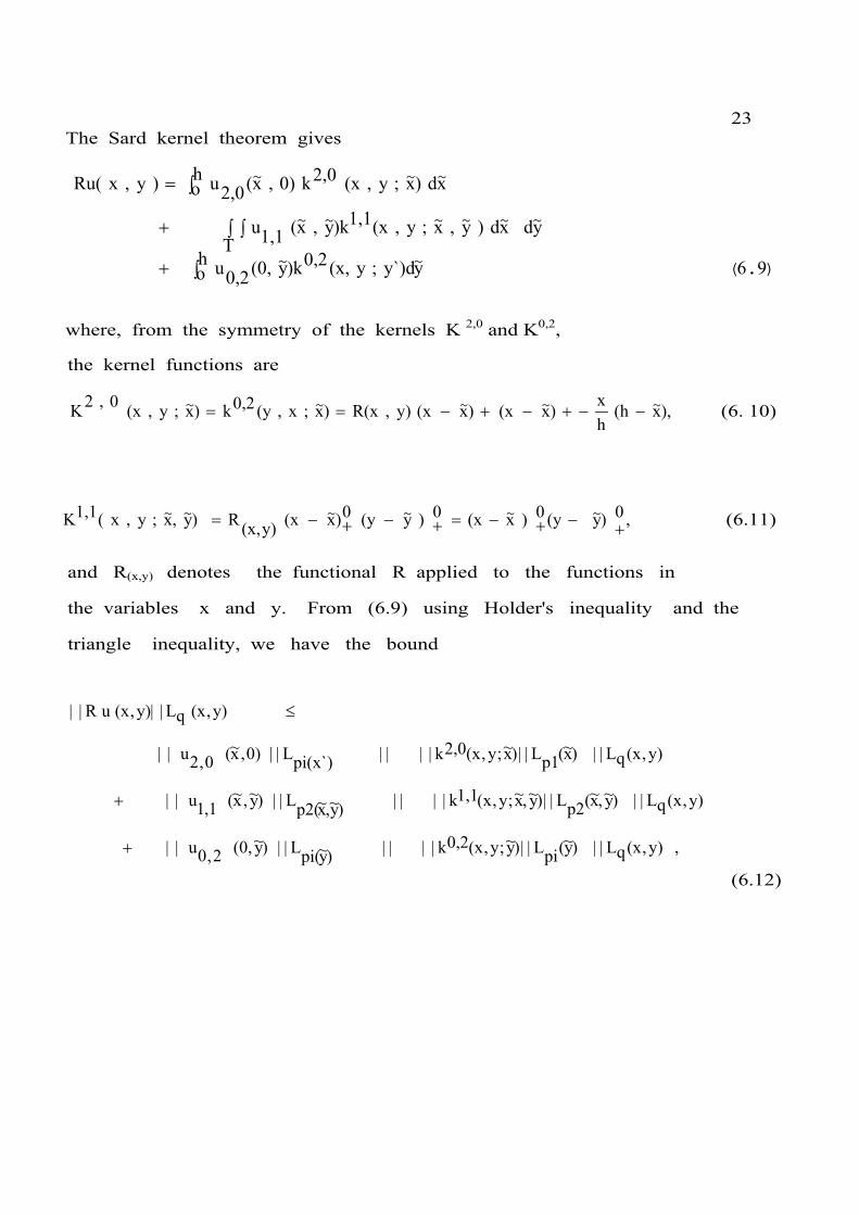
23 The Sard kernel theorem gives

).(~~

~~~~~~

~~~

96yy`)d;(x,0,2)ky(0,ho 0,2u

Tydxd)y,x;y,(x1,1)ky,x(1,1u

xd)x;y,(x2,0k0),x(ho 2,0u)y,xRu(

y∫+

∫ ∫+

∫=

where, from the symmetry of the kernels K 2,0 and K0,2,

the kernel functions are

),x(hhx)x(x)x(xy),R(x)x;x,(y0,2k)x;y,(x0,2K ~~~~~ −−+−+−== (6. 10)

(6.11) ,0)y(y0)x(x0)y(y0)x(xy)(x,)y,x;y,x(1,1K +−+−=+−+−= ~~~~~~ R

and R(x,y) denotes the functional R applied to the functions in

the variables x and y. From (6.9) using Holder's inequality and the

triangle inequality, we have the bound

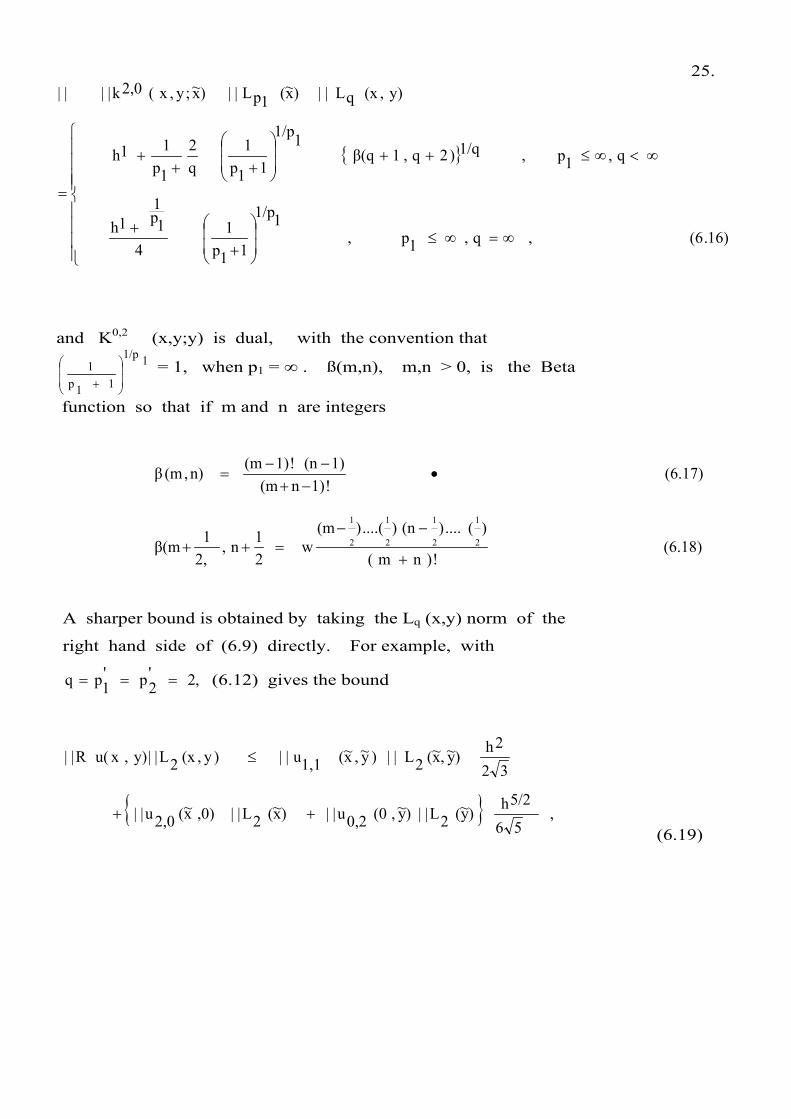
,y),(xqL||)y~(piL||)y~;y,(x0,2k||||)y~pi(L||)y~,(02,0u||

y),(xqL||)y~,x~(p2L||)y~,x~;y,(x1,1k||||)y~,x~p2(L||)y~,x~(1,1u||

y),(xqL||)x~(p1L||)x~;y,(x2,0k||||pi(x`)L||0),x~(0,2u||

y),(xqL||y),(xuR||

+

+

≤

(6.12)

24.

1..2p

1

2p1and1.

1p1

1p1where =+=+ The norms involving

one variable are over [0,h] and those involving two variables

are over T, where, for simplicity, we assume the existence of

the double integral rather than the more general repeated integral

in (6.9). The LP norms of the kernel functions are

(6.14)

,2p,hx)x(h

,1p,1p1

11ph

h

x)x(h

)x~(2Lp||)x~;y,(x2,0k|

(6.13),2p,1

,2p,21/py),(x)y~,x~(

2Lp||)y~,x~;y,(x1,1k||

⎪⎪

⎩

⎪⎪

⎨

⎧

∞=−

∞<⎟⎟

⎠

⎞

⎜⎜

⎝

⎛

+

−

=

⎪⎩

⎪⎨⎧

∞=

∞<=

and K0,2 (x,y:y) is dual. The Lq nortas of (6.13) and (6.14) are

⎪⎪⎪⎪⎪⎪

⎩

⎪⎪⎪⎪⎪⎪

⎨

⎧

∞≤∞=⎟⎟⎠

⎞⎜⎜⎝

⎛

∞=∞<⎟⎟⎠

⎞⎜⎜⎝

⎛

∞<+++

=

⎪⎪⎭

⎪⎪⎬

⎫

⎪⎪⎩

⎪⎪⎨

⎧

⎟⎟⎟⎟

⎠

⎞

⎜⎜⎜⎜

⎝

⎛

⎟⎟⎟⎟

⎠

⎞

⎜⎜⎜⎜

⎝

⎛

(6.15) ,q,2P,1/q

2

2h

,q,2P,21/p

4

2h

,q,2p1/q

22pq,1

2pqβq

12p12

h

y)(x,qL||)y~,x~(2pL||)y~,x~y;(x,1,1k||||

25.

⎪⎪⎪⎪

⎩

⎪⎪⎪⎪

⎨

⎧

∞=∞≤⎟⎟

⎠

⎞

⎜⎜

⎝

⎛

++

∞<∞≤++⎟⎟

⎠

⎞

⎜⎜

⎝

⎛

+++

=

16).(6,q,1p,11/p

11p1

41p1

1h

q,1p, 1/q)2q,1β(q11/p

11p1

q2

1p11h

y),(xqL||)x~(1pL||)x~;y,x(2,0k||||

and K0,2 (x,y;y) is dual, with the convention that 11/p

11p1

⎟⎟

⎠

⎞

⎜⎜

⎝

⎛

+ = 1, when p1 = ∞ . ß(m,n), m,n > 0, is the Beta

function so that if m and n are integers

(6.18)!)nm(

)(....)(n)....()(mw

21n,

2,1β(m

(6.17)!1)n(m1)(n!1)(mn),(mβ

2

1

2

1

2

1

2

1

+

−−=++

•−+

−−=

A sharper bound is obtained by taking the Lq (x,y) norm of the

right hand side of (6.9) directly. For example, with

,2'2p'

1pq === (6.12) gives the bound

,56

5/2h)y~(2L||)y~,(00,2u||)x~(2L||,0)x~(2,0u||

32

2h)y~,x~(2L||)y~,x~(1,1u||)y,(x2L||y),xu(R||

++

≤

(6.19)

26. whereas talcing the L2(x,y) norm directly gives

(6.20)21

64/3

9/2πh)y(2L||)y,(00,2u||

)x(2L||0),x(2,0u||)y,x(2L||)y,x(1,1u||

5h88)y(2L||)y(0,0,2u||)x(2

L||,0)x(2,0u||

180

5h2)y(2L||)y(0,0,2u||2

)x(2L||,0)x(2,0u||

12

4h2)y,x(2L||)y,x(1,1u||y)(x,2L||y)Ru(x,||

⎥⎥⎦

⎤

⎭⎬⎫

+

+

+

⎭⎬⎫

⎩⎨⎧

++

⎢⎣⎡ ≤

~~

~~~~~~

~~~~

~~~~

~~~~

The apparent discrepancy In the orders h is implict in the

difference between the univariate and bivariate norms.

L2 Bounds on R1,0 and R0,1 for Linear Interpolation.

R1,0 and R0,1 are symmetric functionals in ..(T). 1,1B=

The functional

R1,0 u(x,y) = u1,0 (x,y) + h

0),(huu(0,0 −) (6.21)

is zero for the functions 1 ,x, and y. The application of this

functional to the Taylor expansion (6.9) in the Sard space

B1,1 gives

(6.22).yd)y(0,y

0 0,2)uy(yy)(x,1,0R

ydxdy

0)y,x(

x

0 1,1uy)(x,,01R

x,0)dx(x

o 2,0)ux(xy)(x,,01Ry)u(x,1,0R

⎥⎦

⎤⎢⎣

⎡∫ −+

⎥⎦

⎤⎢⎣

⎡∫ ∫+

⎥⎦⎤

⎢⎣⎡∫ −=

~~~

~~~~

~~~

27. R1,0 is not an admissible functional for the Sard kernel

theorem in but the first and last terms in (6.22) can be 1,1B=

evaluated in Sard kernel form. Thus

(6.23)xd)x;y,(x,2,0,0)Kx(h

0 2,0uxd,0)x(x

0 2,0)ux(x1,0R ~~~~~~ ∫=⎥⎦

⎤⎢⎣

⎡∫ −

and

(6.24)yd)x;y,(x,0,2)Ky(0,h

0 0,2uyd)y(0,y

0 0,2)uy(y1,0R ~~~~~~ ∫=⎥⎦

⎤⎢⎣

⎡∫ −

Where

(6.25)x,x,h

xh0)x(x)x(x1,0R)xy;(x,2,0K ≠−

−+−=+−= ~~

~~~

and

0)y(y1,0R)y;(x,0,2k =+−= ~~y (6.26)

For the first kernel xx =~ is a jump set. The second kernel is an

example of the Zero Kernel Theorem. The Lp norm of the kernel

function (6.25) is

⎪⎪

⎩

⎪⎪

⎨

⎧

∞=

∞<⎥⎥

⎦

⎤

⎢⎢

⎣

⎡ +⎟⎠⎞

⎜⎝⎛ −+

+⎟⎟⎠

⎞⎜⎜⎝

⎛+=

(6.27)pif1

1/p

p,

1p

hx1hph

1px1/p

1p1

)x~(pL||)x~;y,(x0,2k||

The middle term of (6.22) is evaluated by applying the functional

directly to it. Thus

(6.28),y)dy(x,y

0 1,1u

xdydx

0)y,x(

y

0 1,1ux

ydxdy

0)y,x(

x

0 1,1u1,0R

~~

~~~~~~~~

∫=

∫ ∫∂∂

=⎥⎦

⎤⎢⎣

⎡∫ ∫

28.

where we have assumed the existence of the double integral so

that Fubini'a theorem applies. Substitution in (6.22) gives

the following!

y)(x,

2L||)x(1PL||)xy;(x,2,0K||||)x('1

Lp||,0)x(2,0u||

y)(x,2L||y)u(x,1,0R||

~~~~

≤

(6.29),y)(x,

2L||yd)y(x,y

0 1,1u|| ~~∫+

Now1'1p

1

1P1Where =+

∫ ∫−

∫h

0

yh

0dydx2yd)y(x,

y

0 1,1u ~~

).(~~

306dydx

'22/p

yd'2p

h

0

yh

0

y

0)yu1,1(x,y2/P2

⎭⎬⎫

∫ ∫−

⎩⎨⎧∫≤

and12P1

2P1Where =+

29

dydx

2/P2yh

0

y

0ydP)yu1,1(x,∫

−

⎭⎬⎫

⎩⎨⎧∫ ~~

'22/P

dxyd'2pyh

0

y

0)y(x,1,1u

'2P

21

y)(h⎪⎭

⎪⎬⎫

⎪⎩

⎪⎨⎧

∫−

∫

−

−≤ ~~

(6.31))y(x,2'2pL

||)y(x,1,1u||1

2P2

y)(h ~~−

−≤

getthusWe2.'2P Provided ≥

y)(x,2L||yd)y(x,)y(x,

y

0 1,1u|| ~~~∫

( )[ ]

⎪⎪⎪

⎩

⎪⎪⎪

⎨

⎧

∞

∞<≤+

≤

).(~~

~~

326)y(x,L||)y(x,1,1u||32

2h

,2P2),y(x,'2P

L||)yu1,1(x,||21

1P22,P2

2β2/P2h

Where ß(m,n) is the Beta function Lastly

.

P,2

h

(6.33)2,P,

222

3h

1,P,152112h

y)(x,2L||)x(1PL||)xy;(x,2,0K||||

⎪⎪⎪⎪

⎩

⎪⎪⎪⎪

⎨

⎧

∞=

=

=

=~~

The L2 bound on R0,1 u (x,y) is dual

30

Application to Finite Element Error Bounds

We consider the space of piecewise linear interpolants over a

triangulated polygon Ω. This is a suitable sub space vh of for 12w

the Galerkin method described in section 2. For a particular

Triangle Te in Ω, a bound on can)e(T12Wy)(x,

~uy)u(x, −

be obtained from (6.12) and (6.29) with a suitable change of

variable from T to Te . error bound is then given by Ω)( 1AW 2

.eTe

Ωwhere

,21

2)e(T1

2Wy)(x,

~uy)u(x,

eΩ) (1

2Wy)(x,~uy)u(x,

∑=

⎪⎭

⎪⎬⎫

⎪⎩

⎪⎨⎧

−∑=−

(6.34)

L2 Bound on R for Quadratic Interpolation

The error functional R u(x,y) = u(x,y) - u(x,y),

where u(x,y) is the quadratic interpolant (6.2), is zero for the

functions 1 , x, y, x2 , xy and y2 • We thus consider the Sard

space B 2,1. (T). The kernel theorem is

,~y)d

~yy;(x,0,3)k

~y(0,0,3uh

o

~y)d

~yy;(x,1,2)k

~y(0,1,2uh

o

~yd

~xd)

~y,

~xy;(x,2,1)k

~y,

~x(2,1u

T

~xd)

~xy;(x,3,0,0)k

~x(3,0uh

oy)Ru(x,

∫+

∫+

∫∫+

∫=

(6.35)

(31)

where the kernel functions are the following

(6.39)

,4xh3213h2x

32112h3x

1625h4x

41555x

h

6x27

2h

7x151o

x2h

4xh1613h2x2h3x

1677h4x

883511x

h

6x2

112h

7x301

)!x(2

2L~xy;(x,3,0k

arefunctionskerneltheofnorms2LtheofsquareThe

(6.38).h2y~

y2h~

y)(yx)~yx(yy)(x,R)

~yy;(x,1,2k

(6.37),2h

4xyo~y

2h~

x2ho)

~y(y)

~x(x

o)~y(y)

~x(xy)(x,R)

~y,

~xy;(x,2,1k

(6.36),2h

22xhx(2))

~x(h2h

24xh4x(2)~

x2h(2))

~x(x

(2))~x(xy)(x,R)

~xx;(y,0,3k)

~xy;(x,3,0k

⎥⎥⎦

⎤

⎢⎢⎣

⎡+−+−+−

+⎟⎠⎞

⎜⎝⎛ −+

⎥⎥⎦

⎤

⎢⎢⎣

⎡−+−+−+−=

⎥⎦

⎤⎢⎣

⎡

+⎟⎠⎞

⎜⎝⎛ −−+−=+−=

+⎟⎠⎞

⎜⎝⎛ −

+⎟⎠⎞

⎜⎝⎛ −−+−+−=

+−+−=

⎥⎥⎦

⎤

⎢⎢⎣

⎡+−−−

⎥⎥⎦

⎤

⎢⎢⎣

⎡−

+⎟⎠⎞

⎜⎝⎛ −−+−=

+−==

32

2y2x31y3x

31)y,x(2

2L||)y,xy;(x,2,1K|| +=~~~~

y3xh

y4x320

2hy

0x

2h

h

2y3x22h

2y4x340

y2h0

x2h

−+⎟⎠⎞

⎜⎝⎛ −

+⎟⎠⎞

⎜⎝⎛ −+

⎥⎥⎦

⎤

⎢⎢⎣

⎡−

+⎟⎠⎞

⎜⎝⎛ −

+⎟⎠⎞

⎜⎝⎛ −+

(6.40),h2xy612y2x

0y

2h0

2hx ⎥⎦

⎤⎢⎣⎡ +−

+⎟⎠⎞

⎜⎝⎛ −

+⎟⎠⎞

⎜⎝⎛ −+

⎥⎥⎦

⎤

⎢⎢⎣

⎡+−

+⎟⎠⎞

⎜⎝⎛ −= h2y

613y

32

h

4y322x

0y

2h)y(2

2L||yy;(x,1,2K|| ~~

(6.41),2yh121h2y

313y

312x

0

2hy ⎥⎦

⎤⎢⎣⎡ +−

+⎟⎠⎞

⎜⎝⎛ −+

and K0,3 ( yy;x, ~) is the dual of K3,0 ( )xyx ~;, .The L2 (x,y) norms

are

(6.44).27h

3·5·753·2

119y)(x,2L||y)(x,2L||)y(2L||)yy;(x,1,2K||||

(6.43),3h3.5.7.2·43·2

761y)(x,2L||)y,x(2L||)y,xy;(x,2,1K||||

(6.42),27h

3.65·3.2

179y)(x,2L||)x(2L||)xy;(x,3,0K||||

=

=

=

~~

~~~~

~~

33

We thus have the bound. :

27

h3·65·3·2

179)y(2L||)y(0,0,3u||)x(2L||,0)x(,03u||y)(x,2L||y)u(x,R||⎭⎬⎫

⎩⎨⎧ +≤ ~~~~

3h3·5·7·2·43·2

761)y,x(2L||)y,x(2,1u|| ~~~~+

(6.45)27h

3·5·753·2

119)y(2L||)y(0,1,2u|| ~~+

We summarise Some results for the quadratic interpolant

Functionals R1,0 and R 0,1 :

The Functional R1 0 for Quadratic Interpolation The functional

(6.46)y2h

4)2h

2,hu(x2h

4h1u(h,0)

y2h

4)2hu(0,x2h

8y2h

4h4,0

2hu

x2h

4y2h

4h3u(0,0)y)(x,1,0uy)u(x,1,0R

−⎥⎦

⎤⎢⎣

⎡+−−

+⎥⎦

⎤⎢⎣

⎡−−⎟

⎠⎞

⎜⎝⎛−

⎥⎦

⎤⎢⎣

⎡++−−=

is admissible for the Sard kernel theorem in The kernel 1,2B=

34.

theorem is

(6.47)y~d)y~;y,(x,30K)y~,0(3,0u

y~d)y~;y,(x,21k)y~,(oho 2,1u

y~dx~d)y~,x~;y,(xT

1,2k)y~,x~(1,2u

x~d)x~;y,(x0,3k0),x~(ho ,03uy)u(x,0,1R

∫+

∫+

∫ ∫+

∫=

where the kernel functions are the following:

(6.48)2h

4xh1(2))x(h2h

8xh4x

2h)x(x)xy;(x,3,0K ⎥

⎦

⎤⎢⎣

⎡+−−−⎥

⎦

⎤⎢⎣

⎡−

+⎟⎠⎞

⎜⎝⎛ −−+−= ~~~~

(2)

(6.49)x,x,2h

4y0y

2hx

2h0)y(y0)x(x)y,xy;(x,2,1K ≠

+⎟⎠⎞

⎜⎝⎛ −

+⎟⎠⎞

⎜⎝⎛ −−+−+−= ~~~~~~~

(6.50),h2yy

2h)y(y)yy;(x,1,2K

+⎟⎠⎞

⎜⎝⎛ −−+−= ~~~

(6.51).0)yy;(x,0,3K =~

The square of the L2 norms of the kernel functions are

(6.52),3h4812xh

83h2x

320

2hx3x

h

4x20

x2h

3h24232xh

1057h2x

51232x

h

4x1217

2h

5x2)x~(2L||)x~;y,(x,03k||

⎥⎦

⎤⎢⎣

⎡−+−

+⎟⎠⎞

⎜⎝⎛ −+

⎥⎥⎦

⎤

⎢⎢⎣

⎡+−

+⎟⎠⎞

⎜⎝⎛ −+

−+−−+−=

35

2y

31xy)y,x(2

2L||)y,xy;(x,2,1K|| +=~~~~

⎥⎥⎦

⎤

⎢⎢⎣

⎡−

+⎟⎠⎞

⎜⎝⎛ −

+⎟⎠⎞

⎜⎝⎛ −+ 2h

2y2x4h

2xy40

y2h0

x2h

⎥⎥⎦

⎤

⎢⎢⎣

⎡−

+⎟⎠⎞

⎜⎝⎛ −

+⎟⎠⎞

⎜⎝⎛ −+

hy2x22xy

0

2hy

0x

2h

(6.53),2y0

y2h0

2hx

+⎟⎠⎞

⎜⎝⎛ −

+⎟⎠⎞

⎜⎝⎛ −−

3yh

4y320

y2h2h2y

613y

312

)y(2L||)yy;(x,1,2K|| −+⎟⎠⎞

⎜⎝⎛ −++=~~

(6.54).2yh121h2y

410

2hy ⎥⎦

⎤⎢⎣⎡ +−

+⎟⎠⎞

⎜⎝⎛ −+

The Functional R0,1 . for Quadratic Interpolation

The functional

⎥⎦

⎤⎢⎣

⎡++−−= y2h

4x2h

4h3u(0,0)y)(x,0,1uy)u(x,0,1R

⎥⎦

⎤⎢⎣

⎡−−⎟

⎠⎞

⎜⎝⎛−⎟

⎠⎞

⎜⎝⎛+ y2h

8x2h

4h4

2h0,ux2h

4,02hu

(6.55)x2h

42h

2,huy2h

4h1h)u(0, ⎟

⎠

⎞⎜⎝

⎛−⎥

⎦

⎤⎢⎣

⎡+−−

36 is not admissible for the Sard kernel theorem in . The 2,1B=application of this functional to the Taylor expansion in 2,1B=gives

⎥⎦

⎤⎢⎣

⎡∫ −= xd,0)x(3,0ux

0(2))x(xy)(x,1,0Ry)u(x,0,1R ~~~

⎥⎦

⎤⎢⎣

⎡∫ ∫ − ydxd)y,x(2,1uy

0)y,x(

x

0 2,1)ux(xy)(x,1,0R ~~~~~~~

⎥⎦

⎤⎢⎣

⎡∫ − yd)y(0,1,2uy

0)y(yxy)(x,1,0R ~~~

).(~~~ 566yd)y(0,0,3u(2)y

0)y(yy)(x,1,0R

⎥⎥

⎦

⎤

⎢⎢

⎣

⎡∫ −

The second term of (6.54) is evaluated by direct application

of the functional to it. Thus

⎥⎦

⎤⎢⎣

⎡∫ ∫ − ydxdy

0)y,x(

x

0 2,1u)x(xy)(x,0,1R ~~~~~

ydxd)y,x(2

h

0 2,1u2

h

0x

2hx2h

4ydxd)y,x(2,1uy

0

x

0)x(x

y~~~~~~~~~~ ∫ ∫ ⎟

⎠⎞

⎜⎝⎛ −−⎥

⎦

⎤⎢⎣

⎡∫ ∫ −

∂∂

=

(6.57).ydxd)y,x(2

h

0 2,1u2

h

0x

2hx2h

4xd)y(x,x

0 2,1)ux(x ~~~~~~~~ ∫ ∫ ⎟⎠⎞

⎜⎝⎛ −−∫ −=

37.

The remaining terms of (6.56) can be evaluated in Sard kernel

form. Thus

(6.58),xd)xy;(x,3,0K,0)x(h

0 3,0uxd,0)x(3,0ux

0(2))x(xy)(x,0,1R ~~~~~~ ∫=⎥

⎦

⎤⎢⎣

⎡∫ −

(6.59),yd)yy;(x,1,2K)y(0,h

0 1,2uyd)y(0,1,2uy

0)y-(yxy)(x,0,1R ~~~~~~ ∫=⎥

⎦

⎤⎢⎣

⎡∫

(6.60)y)dyy;(x,0,3)Ky(0,h

0 0,3uyd)y(0,0,3uy

0(2))y(yy)(x,0,1R ~~~~~~ ∫=⎥

⎦

⎤⎢⎣

⎡∫ −

where the kernel functions are

K3,0 )x~;y,(x = 0 , (6.61)

,yy,h2y

2h0)y(yx)y(x,1,2K ≠⎥

⎦

⎤⎢⎣

⎡

+⎟⎠⎞

⎜⎝⎛ −−+−= ~~~~y (6.62)

)y~;y, )y(x is the dual of the R1,0 kernel K3,0 ~and K 0,3 ;y,(x ,

equation (6.48).

The square of the L2 norm of (6.62)is

h2x61y2x)y(2

2L||yy;(x,1,2K|| +=~~

(6.63)h2x0

2hyy22x

h

2y2x20

y2h

+⎟⎠⎞

⎜⎝⎛ −−

⎥⎥⎦

⎤

⎢⎢⎣

⎡−

+⎟⎠⎞

⎜⎝⎛ −+

A L2 (x,y) bound on R1,0 u(x,y) and R0,1 u(x,y) can be

obtained as was done above for the functional R.

Acknowledgment. The authors wish to acknowledge helpful discussions with J. R. Whiteman.

38.

39,

References

1. Barnhill R.E., and Pilcher D.T., Sard kernels for certain bivariate cubatures. Technical Report 4, Department of Mathematics, Brunei University, 1971.

2. Barnhill R.E. and Whiteman J.R., Error analysis of finite element methods with triangles for elliptic boundary value problems. In whiteman,j.R.ed.),The Mathematics of Finite Elements and Applications, Academic Press, London,1972.

3. Barnhill R.E., and Whiteman J.R., Computable error bounds for the finite element method for elliptic boundaiy value problems. In L.Collatz (ed,),Proceedings of the Symposium on Numerical Solution of Differential Equationa, Oberwolfach, Germany, 1972.

4. Birkhoff G., Schultz M.H., and Varga R.E., Piecewise Hermite interpolation in one and two variables with applications to partial differential equations. Numerischs Mathematik 11, 232-256, 1968.

5. Davis P.J., Interpolation and Approximation. Blaisdell, New York, 1962.

6. Sard A., Linear Approximation, Matheniatical Survey 9, American Mathematical Society, Providence, Rhode Island, 1963.

7. Smirnov V.I., A Course of Higher Mathematics, Vol.V. Pergamon Press, Oxford, 1964.

8. Stancu D.D., The remainder of certain linear approximation formulas in two variables. SIAM Journal on Numerical Analysis 1, 137-163, 1964.

9. Strang G., Approximation in the finite element method. Numerische Mathematik 19, 81-98,1972.

10. Stroud A.H., Approximate Calculation of Multiple Integrals. Prentice-Hall, 1971.

11. Varga R.S., The role of interpolation and approximation theory in variational and projectional methods for solving partial differential equations. IFIP Congress 71, 14 -19, North Holland Amsterdam, 1971.

12. Zenisek A., Interpolation polynomials on the triangle. Numer.Math.15, 282-296, 1970.

13. Zlamal M., On the finite element method. Numer.Math. 12, 394-409, 1968.

14. Zlamal M., Some recent advances in the mathematics of finite elements. In Whiteman (ed.) The Mathematics of Finite Elements and Applications, 59-81, Academic Press, London, 1972.

15. Bramble J.H., and Zlamal M., Triangular elements in the finite element method. Math.Comp.24,809-820, 1970.