ETSI TR 102 376-2 V1.1.1 (2015-11)

Digital Video Broadcasting (DVB); Implementation guidelines for the second generation system for Broadcasting, Interactive Services, News Gathering and

other broadband satellite applications; Part 2: S2 Extensions (DVB-S2X)

TECHNICAL REPORT

�

ETSI

ETSI TR 102 376-2 V1.1.1 (2015-11)2

Reference DTR/JTC-DVB-354-2

Keywords broadband, broadcasting, digital, satellite, TV,

video

ETSI

650 Route des Lucioles F-06921 Sophia Antipolis Cedex - FRANCE

Tel.: +33 4 92 94 42 00 Fax: +33 4 93 65 47 16

Siret N° 348 623 562 00017 - NAF 742 C

Association à but non lucratif enregistrée à la Sous-Préfecture de Grasse (06) N° 7803/88

Important notice

The present document can be downloaded from: http://www.etsi.org/standards-search

The present document may be made available in electronic versions and/or in print. The content of any electronic and/or print versions of the present document shall not be modified without the prior written authorization of ETSI. In case of any

existing or perceived difference in contents between such versions and/or in print, the only prevailing document is the print of the Portable Document Format (PDF) version kept on a specific network drive within ETSI Secretariat.

Users of the present document should be aware that the document may be subject to revision or change of status. Information on the current status of this and other ETSI documents is available at

http://portal.etsi.org/tb/status/status.asp

If you find errors in the present document, please send your comment to one of the following services: https://portal.etsi.org/People/CommiteeSupportStaff.aspx

Copyright Notification

No part may be reproduced or utilized in any form or by any means, electronic or mechanical, including photocopying and microfilm except as authorized by written permission of ETSI.

The content of the PDF version shall not be modified without the written authorization of ETSI. The copyright and the foregoing restriction extend to reproduction in all media.

© European Telecommunications Standards Institute 2015.

© European Broadcasting Union 2015. All rights reserved.

DECTTM, PLUGTESTSTM, UMTSTM and the ETSI logo are Trade Marks of ETSI registered for the benefit of its Members.

3GPPTM and LTE™ are Trade Marks of ETSI registered for the benefit of its Members and of the 3GPP Organizational Partners.

GSM® and the GSM logo are Trade Marks registered and owned by the GSM Association.

ETSI

ETSI TR 102 376-2 V1.1.1 (2015-11)3

Contents Intellectual Property Rights ................................................................................................................................ 8

Foreword ............................................................................................................................................................. 8

Modal verbs terminology .................................................................................................................................... 8

1 Scope ........................................................................................................................................................ 9

2 References ................................................................................................................................................ 9

2.1 Normative references ......................................................................................................................................... 9

2.2 Informative references ........................................................................................................................................ 9

3 Symbols and abbreviations ..................................................................................................................... 11

3.1 Symbols ............................................................................................................................................................ 11

3.2 Abbreviations ................................................................................................................................................... 12

4 General description of the technical characteristics of the DVB-S2X extensions ................................. 15

4.0 Overview .......................................................................................................................................................... 15

4.1 Commercial requirements ................................................................................................................................ 15

4.1.0 Background ................................................................................................................................................. 15

4.1.1 Use Cases for an enhanced DVB-S2 Standard ........................................................................................... 16

4.1.1.0 General aspects ..................................................................................................................................... 16

4.1.1.1 Direct-to-Home ..................................................................................................................................... 16

4.1.1.2 Applications requiring low SNR links .................................................................................................. 16

4.1.2 Commercial requirements for the enhancements of the DVB-S2 standard ................................................ 16

4.2 Application scenarios ....................................................................................................................................... 18

4.3 System architecture .......................................................................................................................................... 19

4.3.0 General ........................................................................................................................................................ 19

4.3.1 CRC8_MODE computation in GSE High Efficiency Mode (GSE-HEM) ................................................. 19

4.3.2 Signalling of the DVB-S2X MODCODs .................................................................................................... 19

4.3.3 Roll off detection on DVB-S2X ................................................................................................................. 20

4.3.4 Reference performance ............................................................................................................................... 21

4.4 Channel models ................................................................................................................................................ 24

4.4.0 Introduction................................................................................................................................................. 24

4.4.1 DTH Broadcasting services ........................................................................................................................ 25

4.4.1.0 General description ............................................................................................................................... 25

4.4.1.1 Uplink station HPA ............................................................................................................................... 27

4.4.1.2 IMUX and OMUX filters ...................................................................................................................... 27

4.4.1.3 Cross-polar interference models............................................................................................................ 29

4.4.1.3.0 General description .......................................................................................................................... 29

4.4.1.3.1 Satellite antenna polarization discrimination ................................................................................... 29

4.4.1.3.2 Depolarization ................................................................................................................................. 29

4.4.1.3.3 User terminal outdoor unit polarization isolation ............................................................................ 30

4.4.1.3.4 Cross-polarization summary model ................................................................................................. 31

4.4.1.4 On-board TWTA ................................................................................................................................... 31

4.4.1.5 Interference Scenarios for the evolutionary path................................................................................... 33

4.4.1.5.0 Overview ......................................................................................................................................... 33

4.4.1.5.1 Adjacent Satellite Interference ........................................................................................................ 34

4.4.1.6 Phase and Frequency Errors .................................................................................................................. 36

4.4.1.6.1 Phase noise ...................................................................................................................................... 36

4.4.1.6.2 Carrier Frequency instabilities ......................................................................................................... 38

4.4.1.7 Receiver Amplitude Distortions ............................................................................................................ 38

4.4.1.8 Fading Dynamics .................................................................................................................................. 38

4.4.2 VSAT Outbound ......................................................................................................................................... 39

4.4.2.1 Scenarios ............................................................................................................................................... 39

4.4.2.1.1 Single Beam in Ku-band.................................................................................................................. 39

4.4.2.1.2 Multi-spot beam in Ka-band ............................................................................................................ 39

4.4.2.1.2.0 General description of the scenarios .......................................................................................... 39

4.4.2.1.2.1 71 beams with a 4 colours scheme ............................................................................................. 40

4.4.2.1.2.2 71 beams with a 2 colours scheme ............................................................................................. 42

4.4.2.1.2.3 200 beams with a 4 colours scheme and 500 MHz of total user bandwidth .............................. 44

ETSI

ETSI TR 102 376-2 V1.1.1 (2015-11)4

4.4.2.1.2.4 200 Beams with a 4 colours scheme and 3 GHz of total user bandwidth .................................. 46

4.4.2.2 VSAT Forward Links in regions prone to deep transient atmospheric fading ...................................... 47

4.4.2.3 Channel models for the VSAT outbound scenarios .............................................................................. 48

4.4.2.3.0 Introduction ..................................................................................................................................... 48

4.4.2.3.1 Single beam in Ku-band .................................................................................................................. 48

4.4.2.3.2 Multi-carrier per TWTA and high number of colours (negligible co-channel interference) ........... 48

4.4.2.3.2.0 General description .................................................................................................................... 48

4.4.2.3.2.1 GW HPA .................................................................................................................................... 49

4.4.2.3.2.2 IMUX and DIPLEXER filters.................................................................................................... 50

4.4.2.3.2.3 On-board TWTA ........................................................................................................................ 50

4.4.2.3.2.4 Phase and Frequency Errors ....................................................................................................... 50

4.4.2.3.2.5 Receiver Amplitude Distortions................................................................................................. 50

4.4.2.3.3 Single Carrier per TWTA and 2 colours .......................................................................................... 50

4.4.2.3.3.0 General description .................................................................................................................... 50

4.4.2.3.3.1 GW HPA .................................................................................................................................... 51

4.4.2.3.3.2 IMUX and User Bandwidth Filter ............................................................................................. 52

4.4.2.3.3.3 TWTA ........................................................................................................................................ 52

4.4.2.3.3.4 Co-channel Interference Model ................................................................................................. 52

4.4.2.3.3.5 Phase and Frequency Error ........................................................................................................ 52

4.4.2.3.3.6 Receiver Amplitude Distortions................................................................................................. 52

4.4.2.4 Phase Noise Masks ................................................................................................................................ 52

4.4.3 Broadcast Distribution, Contribution and High Speed IP links .................................................................. 54

4.4.3.0 Introduction ........................................................................................................................................... 54

4.4.3.1 Notes on optimization criteria for contribution links ............................................................................ 54

4.4.3.1.0 Introduction ..................................................................................................................................... 54

4.4.3.1.1 Example of Link Budget over an Existing Satellite......................................................................... 54

4.4.3.2 A Channel Model for Contribution Links ............................................................................................. 57

4.4.3.2.0 General description .......................................................................................................................... 57

4.4.3.2.1 GW HPA ......................................................................................................................................... 59

4.4.3.2.2 IMUX and OMUX Filter ................................................................................................................. 59

4.4.3.2.3 On-board TWTA ............................................................................................................................. 59

4.4.3.2.4 Phase and Frequency Errors ............................................................................................................ 59

4.4.3.2.5 Receiver Amplitude Distortions ...................................................................................................... 59

4.4.4 Emerging Mobile Applications (airborne and railway) .............................................................................. 60

4.4.4.0 Introduction ........................................................................................................................................... 60

4.4.4.1 Frequency Stability and Phase Noise .................................................................................................... 60

4.4.4.2 Terminal-Motion Doppler Shift ............................................................................................................ 60

4.4.4.3 Multipath Fading ................................................................................................................................... 61

4.4.4.4 Shadowing ............................................................................................................................................. 61

4.4.4.5 Adjacent Satellite Interference .............................................................................................................. 62

4.4.4.6 SNR Dynamics ...................................................................................................................................... 63

4.4.4.6.0 General description .......................................................................................................................... 63

4.4.4.6.1 Forward Link ................................................................................................................................... 63

4.4.4.6.2 Return Link ...................................................................................................................................... 64

4.4.4.7 Summary of the Channel Models for the Mobile Services ................................................................... 64

4.5 Performance over typical satellite channels ..................................................................................................... 66

4.5.0 Introduction................................................................................................................................................. 66

4.5.1 Reference Receiver Architecture ................................................................................................................ 67

4.5.2 Performance in DTH Broadcasting Services .............................................................................................. 67

4.5.3 Performance in VSAT Outbound ................................................................................................................ 71

4.5.4 Performance in Broadcast Distribution, Contribution and High Speed IP links ......................................... 75

4.6 Channel bonding .............................................................................................................................................. 78

4.6.0 Introduction................................................................................................................................................. 78

4.6.1 The principle and advantages of Channel Bonding .................................................................................... 78

4.6.2 Channel bonding for TS transmissions ....................................................................................................... 79

4.6.3 Channel bonding for GSE transmissions .................................................................................................... 82

4.7 S2X system configurations ............................................................................................................................... 82

5 Broadcast applications ............................................................................................................................ 84

5.0 Introduction ...................................................................................................................................................... 84

5.1 DVB-S2X features for broadcast applications ................................................................................................. 84

5.1.1 Broadcasting with differentiated channel protection .................................................................................. 84

ETSI

ETSI TR 102 376-2 V1.1.1 (2015-11)5

5.1.2 Channel bonding ......................................................................................................................................... 85

5.1.3 Higher order modulation ............................................................................................................................. 85

5.2 Comparative Performance Assessment ............................................................................................................ 85

5.2.0 Introduction................................................................................................................................................. 85

5.2.1 Receiver architecture assumptions .............................................................................................................. 85

5.2.2 Video Service Quality ................................................................................................................................. 86

5.2.3 Example Scenario 1: Ku-band broadcasting with a wide coverage ............................................................ 86

5.2.3.0 Introduction ........................................................................................................................................... 86

5.2.3.1 Study cases for reference scenario 1 ..................................................................................................... 88

5.2.3.1.0 Introduction ..................................................................................................................................... 88

5.2.3.1.1 Study case 1.1: DVB-S2 with legacy receiver and MPEG-4 decoder ............................................. 88

5.2.3.1.2 Study case 1.2: DVB-S2 with enhanced receiver and MPEG-4 decoder ........................................ 88

5.2.3.1.3 Study case 1.3: DVB-S2X with enhanced receiver and MPEG-4 decoder ...................................... 88

5.2.3.1.4 Study case 1.4: DVB-S2 with enhanced receiver and HEVC decoder ............................................ 88

5.2.3.1.5 Study case 1.5: DVB-S2X with enhanced receiver and MPEG-4 decoder ...................................... 88

5.2.3.2 Comparative performance results for reference scenario 1 ................................................................... 90

5.2.4 Example Scenario 2: Ka-band Multi-Beam broadcasting satellite ............................................................. 91

5.2.4.0 General .................................................................................................................................................. 91

5.2.4.1 Study cases for reference scenario 2 ..................................................................................................... 93

5.2.4.1.0 Introduction ..................................................................................................................................... 93

5.2.4.1.1 Study case 2.1: Ku-band reference system with DVB-S2 and legacy receiver ............................... 93

5.2.4.1.2 Study case 2.2: Ku-band reference system with DVB-S2 and enhanced receiver ........................... 93

5.2.4.1.3 Study case 2.3: Ku-band reference system with DVB-S2X with channel bonding ......................... 93

5.2.4.1.4 Study case 2.4: Ka-band system with DVB-S2 and enhanced receiver ........................................... 93

5.2.4.1.5 Study case 2.5: Ka-band system with DVB-S2X ............................................................................ 93

5.2.4.1.6 Study case 2.6: Ka-band system with DVB-S2X and 97,0 % UHD availability ............................. 93

5.2.4.2 Comparative performance results for reference scenario 2 ................................................................... 95

6 Interactive applications........................................................................................................................... 96

6.0 Introduction ...................................................................................................................................................... 96

6.1 Performance over next generation multi-beam broadband systems ................................................................. 97

6.1.0 General ........................................................................................................................................................ 97

6.1.1 200 multi-spot beam European scenario ..................................................................................................... 99

6.1.1.0 Description of the scenario .................................................................................................................... 99

6.1.1.1 Baseline performance with DVB-S2, roll-off 20 % ............................................................................ 100

6.1.1.2 Performance with DVB-S2X, roll-off 20 % ........................................................................................ 102

6.1.1.3 Performance with DVB-S2X, roll-off 5 % .......................................................................................... 103

6.1.2 40 multi-spot beam regional scenario ....................................................................................................... 104

6.1.2.0 Description of the scenario .................................................................................................................. 104

6.1.2.1 Baseline performance with DVB-S2, roll-off 20 % ............................................................................ 105

6.1.2.2 Performance with DVB-S2X, roll-off 20 % ........................................................................................ 107

6.1.2.3 Performance with DVB-S2X, roll-off 5 % .......................................................................................... 107

6.1.3 Conclusions on the performance of DVB-S2X for next generation broadband networks ........................ 109

7 Contribution services, data content distribution/trunking and other professional applications ............ 109

8 VL-SNR applications ........................................................................................................................... 111

8.0 Introduction .................................................................................................................................................... 111

8.1 Operation in Heavy Fade Conditions ............................................................................................................. 111

8.2 Small-Aperture Antenna Reception................................................................................................................ 113

8.3 Contribution Links Originating from Small-Aperture Terminals ................................................................... 114

Annex A: Linear MODCODs .............................................................................................................. 116

Annex B: DVB-S2X VL-SNR Modes ................................................................................................. 117

B.1 VL-SNR MODCODs ........................................................................................................................... 117

B.2 VL-SNR Frame and pilot structure ...................................................................................................... 122

B.3 VL-SNR MODCOD Signalling ........................................................................................................... 123

B.4 VL-SNR Dummy Frames ..................................................................................................................... 126

Annex C: Super-Framing structure ................................................................................................... 128

ETSI

ETSI TR 102 376-2 V1.1.1 (2015-11)6

C.0 General description............................................................................................................................... 128

C.1 Application Scenarios and System Setup ............................................................................................. 129

C.1.0 Introduction to Super-Frame Formats ............................................................................................................ 129

C.1.1 Focus of Super-Frame Formats ...................................................................................................................... 129

C.1.2 Comparison of Super-Frame Format Features ............................................................................................... 130

C.1.3 Application Scenario Beam-Hopping/ -Switching ......................................................................................... 131

C.2 Clarifications and Additional Explanations of the Specification ......................................................... 132

C.2.0 General ........................................................................................................................................................... 132

C.2.1 Common Super-Frame Structure .................................................................................................................... 132

C.2.1.1 SF-Scrambler Implementation and Justification for Two-Way Scrambling ............................................. 132

C.2.1.2 Two-Way Scrambler Configuration and SOSF and Pilots Sequence Selection in Interference Scenarios ................................................................................................................................................... 133

C.2.1.3 Padding for 128APSK .............................................................................................................................. 136

C.2.2 Additional information related to Format 0 and 1 .......................................................................................... 136

C.2.3 Additional information related to Format 2 and 3 .......................................................................................... 136

C.2.3.0 General aspects ......................................................................................................................................... 136

C.2.3.1 Implementation of Spreading .................................................................................................................... 136

C.2.4 Additional information related to Format 4 .................................................................................................... 136

C.2.4.1 Modulation and Coding ............................................................................................................................ 136

C.2.4.2 Implementation of Spreading .................................................................................................................... 137

C.2.4.3 VL-SNR operation in connection with CCM/ACM/VCM ....................................................................... 137

C.2.4.4 Use of SID/ISI/TSN of the PLH ............................................................................................................... 137

C.2.4.5 Application of Dummy-Frames ................................................................................................................ 137

C.2.4.6 PLFRAME Mapping into Super-Frame .................................................................................................... 138

C.3 Synchronization to the Super-Frame (independent of content format) ................................................ 140

C.3.0 General aspects ............................................................................................................................................... 140

C.3.1 SF-aided Timing Synchronization .................................................................................................................. 140

C.3.1.1 Conventional approach ............................................................................................................................. 140

C.3.1.2 SOSF + SFFI Assisted Symbol Timing Recovery .................................................................................... 141

C.3.1.3 Probability of SF-lock ............................................................................................................................... 143

C.3.2 SFFI Decoder Performance ............................................................................................................................ 145

C.4 Super-Frame-Format-specific Synchronization Cases ......................................................................... 145

C.4.0 Introduction .................................................................................................................................................... 145

C.4.1 Format 0 and 1 ................................................................................................................................................ 146

C.4.2 Format 2 and 3 ................................................................................................................................................ 146

C.4.3 Format 4 ......................................................................................................................................................... 146

C.4.3.0 Overview .................................................................................................................................................. 146

C.4.3.1 SFH Word Error Rate ............................................................................................................................... 146

C.4.3.2 PLH Word Error Rate ............................................................................................................................... 147

C.5 Example of Exploitation of the Superframing Structure: Precoding in Broadband Interactive Networks .............................................................................................................................................. 150

C.5.1 System Elements for Applying Precoding in Multibeam High Throughput Systems .................................... 150

C.5.1.0 General description ................................................................................................................................... 150

C.5.1.1 System Model & Payload Resources ........................................................................................................ 150

C.5.1.2 Forming the Channel Matrix ..................................................................................................................... 152

C.5.1.3 Algorithms for Multicast Precoding ......................................................................................................... 152

C.5.1.4 Implementation Aspects of Multicast Precoding ...................................................................................... 154

C.5.1.5 Multibeam Satellite System Channel Impairments and Formulation ....................................................... 156

C.5.2 Synchronization Procedure at the Terminal for pre-coded waveforms .......................................................... 158

C.5.2.1 Introduction............................................................................................................................................... 158

C.5.2.2 Signal Model ............................................................................................................................................. 158

C.5.2.3 Synchronization Procedure ....................................................................................................................... 159

C.5.2.3.0 General description ............................................................................................................................. 159

C.5.2.3.1 Synchronization procedure for "Quasi-Synchronous" Signals ............................................................ 159

C.5.2.3.2 Synchronization procedure for "non-synchronous" Signals ................................................................ 160

C.5.2.4 Numerical Examples ................................................................................................................................. 162

C.5.2.4.0 Introduction ......................................................................................................................................... 162

C.5.2.4.1 Discussion on impairments ................................................................................................................. 162

ETSI

ETSI TR 102 376-2 V1.1.1 (2015-11)7

C.5.2.4.2 Numerical results ................................................................................................................................ 163

C.5.2.4.2.0 Assuptions ..................................................................................................................................... 163

C.5.2.4.2.1 Coarse Frequency Acquisition ....................................................................................................... 163

C.5.2.4.2.2 Frame Synchronization and Interferer Frame Synchronization ..................................................... 164

C.5.2.4.2.3 Time tracking and Interferer Time tracking .................................................................................. 165

C.5.2.4.2.4 Channel Estimation ....................................................................................................................... 168

C.5.3 System performance estimation ..................................................................................................................... 168

C.5.3.1 System Overview ...................................................................................................................................... 168

C.5.3.2 Performance Estimation ............................................................................................................................ 169

C.5.3.2.0 General description of the scenarios ................................................................................................... 169

C.5.3.2.1 CSI Errors ........................................................................................................................................... 170

C.5.3.2.2 Outdated CSI information due to phase noise ..................................................................................... 170

C.5.3.2.3 Threshold on weakest user estimate .................................................................................................... 172

Annex D: Time slicing .......................................................................................................................... 174

Annex E: IMUX and OMUX filters characteristics .......................................................................... 175

Annex F: Details for adjacent satellite interference modelling........................................................ 176

Annex G: Phase Noise Model in Computer Simulations .................................................................. 177

G.1 Introduction .......................................................................................................................................... 177

G.2 Definition of phase noise ...................................................................................................................... 177

G.3 Digital synthesis of the phase noise in simulations .............................................................................. 179

Annex H: Bibliography ........................................................................................................................ 181

History ............................................................................................................................................................ 182

ETSI

ETSI TR 102 376-2 V1.1.1 (2015-11)8

Intellectual Property Rights IPRs essential or potentially essential to the present document may have been declared to ETSI. The information pertaining to these essential IPRs, if any, is publicly available for ETSI members and non-members, and can be found in ETSI SR 000 314: "Intellectual Property Rights (IPRs); Essential, or potentially Essential, IPRs notified to ETSI in respect of ETSI standards", which is available from the ETSI Secretariat. Latest updates are available on the ETSI Web server (http://ipr.etsi.org).

Pursuant to the ETSI IPR Policy, no investigation, including IPR searches, has been carried out by ETSI. No guarantee can be given as to the existence of other IPRs not referenced in ETSI SR 000 314 (or the updates on the ETSI Web server) which are, or may be, or may become, essential to the present document.

Foreword This Technical Report (TR) has been produced by Joint Technical Committee (JTC) Broadcast of the European Broadcasting Union (EBU), Comité Européen de Normalisation ELECtrotechnique (CENELEC) and the European Telecommunications Standards Institute (ETSI).

The work of the JTC was based on the studies carried out by the European DVB Project under the auspices of the Ad Hoc Group on DVB-S2 of the DVB Technical Module. This joint group of industry, operators and broadcasters provided the necessary information on all relevant technical matters (see clause 2).

NOTE: The EBU/ETSI JTC Broadcast was established in 1990 to co-ordinate the drafting of standards in the specific field of broadcasting and related fields. Since 1995 the JTC Broadcast became a tripartite body by including in the Memorandum of Understanding also CENELEC, which is responsible for the standardization of radio and television receivers. The EBU is a professional association of broadcasting organizations whose work includes the co-ordination of its members' activities in the technical, legal, programme-making and programme-exchange domains. The EBU has active members in about 60 countries in the European broadcasting area; its headquarters is in Geneva.

European Broadcasting Union CH-1218 GRAND SACONNEX (Geneva) Switzerland Tel: +41 22 717 21 11 Fax: +41 22 717 24 81

The Digital Video Broadcasting Project (DVB) is an industry-led consortium of broadcasters, manufacturers, network operators, software developers, regulatory bodies, content owners and others committed to designing global standards for the delivery of digital television and data services. DVB fosters market driven solutions that meet the needs and economic circumstances of broadcast industry stakeholders and consumers. DVB standards cover all aspects of digital television from transmission through interfacing, conditional access and interactivity for digital video, audio and data. The consortium came together in 1993 to provide global standardisation, interoperability and future proof specifications.

The present document is part 2 of a multi-part deliverable covering the implementation guidelines for the second generation system for Broadcasting, Interactive Services, News Gathering and other broadband satellite applications, as identified below:

Part 1: "DVB-S2";

Part 2: "S2 Extensions (DVB-S2X)".

Modal verbs terminology In the present document "shall", "shall not", "should", "should not", "may", "need not", "will", "will not", "can" and "cannot" are to be interpreted as described in clause 3.2 of the ETSI Drafting Rules (Verbal forms for the expression of provisions).

"must" and "must not" are NOT allowed in ETSI deliverables except when used in direct citation.

ETSI

ETSI TR 102 376-2 V1.1.1 (2015-11)9

1 Scope The present document gives an overview of the technical and operational issues relevant to the system specified in ETSI EN 302 307-2 [i.2], and is intended to provide guidance to broadcasters and operators considering the adoption of DVB-S2X. It is assumed a reasonable familiarity with the original DVB-S2 standard ETSI EN 302 307-1 [i.1], whose technical and operational issues are described in details in ETSI TR 102 376-1 [i.3]. It can also be considered as a useful guideline for implementation of DVB-S2, when enhanced DVB-S2 receivers and channel models are applicable.

2 References

2.1 Normative references References are either specific (identified by date of publication and/or edition number or version number) or non-specific. For specific references, only the cited version applies. For non-specific references, the latest version of the reference document (including any amendments) applies.

Referenced documents which are not found to be publicly available in the expected location might be found at http://docbox.etsi.org/Reference.

NOTE: While any hyperlinks included in this clause were valid at the time of publication, ETSI cannot guarantee their long term validity.

The following referenced documents are necessary for the application of the present document.

Not applicable.

2.2 Informative references References are either specific (identified by date of publication and/or edition number or version number) or non-specific. For specific references, only the cited version applies. For non-specific references, the latest version of the reference document (including any amendments) applies.

NOTE: While any hyperlinks included in this clause were valid at the time of publication, ETSI cannot guarantee their long term validity.

The following referenced documents are not necessary for the application of the present document but they assist the user with regard to a particular subject area.

[i.1] ETSI EN 302 307-1: "Digital Video Broadcasting (DVB); Second generation framing structure, channel coding and modulation systems for Broadcasting, Interactive Services, News Gathering and other broadband satellite applications; Part 1: DVB-S2".

[i.2] ETSI EN 302 307-2: "Digital Video Broadcasting (DVB); Second generation framing structure, channel coding and modulation systems for Broadcasting, Interactive Services, News Gathering and other broadband satellite applications; Part 2: DVB-S2 Extensions (DVB-S2X)".

[i.3] ETSI TR 102 376-1: "Digital Video Broadcasting (DVB) Implementation guidelines for the second generation system for Broadcasting, Interactive Services, News Gathering and other broadband satellite applications; Part 1: DVB-S2".

[i.4] Ken Mc Cann: "Review of DTT HD Capacity Issues, An Independent Report from ZetaCast Ltd Commissioned by Ofcom".

[i.5] ETSI TS 102 991: "Digital Video Broadcasting (DVB); Implementation Guidelines for a second generation digital cable transmission system (DVB-C2)".

[i.6] J. Grotz, B. Ottersten, J. Krause: "Applicability of Interference Processing to DTH Reception", 9th International Workshop on Signal Processing for Space Communications, September 2006.

[i.7] ETSI TR 102 768: "Digital Video Broadcasting (DVB); Interaction channel for Satellite Distribution Systems; Guidelines for the use of EN 301 790 in mobile scenarios".

ETSI

ETSI TR 102 376-2 V1.1.1 (2015-11)10

[i.8] ETSI TR 101 790: "Digital Video Broadcasting (DVB); Interaction channel for Satellite Distribution Systems; Guidelines for the use of EN 301 790".

[i.9] M. Holzbock, E. Lutz, G. Losquadro: "Aeronautical Channel Measurements and Multimedia Service Demonstration at K/Ka Band", 4th ACTS Mobile Communications Summit, Sorrento, Italy, 1999.

[i.10] A. Dissanayake: "Ka-Band Propagation Modeling for Fixed Satellite Applications", Online Journal of Space Communication, Issue number 2, Fall 2002.

[i.11] C. Morlet et. al.: "Implementation of Spreading Techniques in Mobile DVB-S2/DVB-RCS Systems", Proc. IWSSC 2007, Salzburg, Austria, September 2007, pages 259-263.

[i.12] ETSI EN 303 978: "Satellite Earth Stations and Systems (SES); Harmonised EN for Earth Stations on Mobile Platforms (ESOMP) transmitting towards satellites in geostationary orbit in the 27,5 GHz to 30,0 GHz frequency bands covering the essential requirements of article 3.2 of the R&TTE Directive".

[i.13] E. Kubista, F. Perez Fontan, M. A. Vazquez Castro, S. Buonomo, B. R. Arbesser-Rastburg, J.P.V. Poiares Baptista: "Ka-Band Propagation Measurements and Statistics for Land Mobile Satellite Applications", IEEE Transactions on Vehicular Technology, volume 49, number 3, May 2000.

[i.14] F. Perez Fontan, M. Vazquez Castro, C. Enjamio Cabado, J. Pita Garcia, and E. Kubista: "Statistical modelling of the LMS channel", IEEE Transactions on Vehicular Technology", volume 50, pages 1 549-1 567, November 2001.

[i.15] IEEE Std 1139™: "IEEE Standard Definitions of Physical Quantities for Fundamental Frequency and Time Metrology - Random Instabilities", February 2009.

[i.16] F.M. Gardner: "Phaselock Techniques", 3rd edition, Wiley, 2005.

[i.17] W.H. Press, et al.: "Numerical Recipes in C - The Art of Scientific Computing", Cambridge University Press, 2002.

[i.18] A. Ginesi and S. Cioni: "Phase Noise Model in Computer Simulations", ESA Technical Report, December 2013.

[i.19] T. Alberty and V. Hespelt: "A New pattern Jitter Free Frequency Error Detector", IEEE Transactions on Communications, volume 37, number 2, pages 159-163, February 1989.

[i.20] J.G. Proakis, M. Salehi: "Digital Communications", 5th edition, McGraw-Hill, 2008.

[i.21] E. Casini, A. Ginesi, and R. De Gaudenzi: "DVB-S2 modem algorithms design and performance over typical satellite channels", International Journal of Satellite Communications and Networking, volume 22, number 3, pages 281-318, 2004.

[i.22] Zoellner, J.; Loghin, N.: "Optimization of high-order non-uniform QAM constellations", IEEE International Symposium on Broadband Multimedia Systems and Broadcasting (BMSB), June 2013.

[i.23] D'Andrea, A.N.; Mengali, U.: "Design of quadricorrelators for automatic frequency control systems", IEEE Transactions on Communications, volume 41, number 6, pages 988-997, June 1993.

[i.24] Kim, P., Pedone, R., Villanti, M., Vanelli-Coralli, A., Corazza, G. E., Chang, D.-I. and Oh, D.-G. (2009): "Robust frame synchronization for the DVB-S2 system with large frequency offsets", International Journal of Satellite Communications and Networking, 27: 35-52.

[i.25] Pedone, R.; Villanti, M.; Vanelli-Coralli, A.; Corazza, G.E.; Mathiopoulos, P.T.: "Frame synchronization in frequency uncertainty", IEEE Transactions on Communications, volume 58, number 4, pages 1 235-1 246, April 2010.

ETSI

ETSI TR 102 376-2 V1.1.1 (2015-11)11

[i.26] Anzalchi, J.; Couchman, A.; Gabellini, P.; Gallinaro, G.; D'Agristina, L.; Alagha, N.; Angeletti, P.: "Beam hopping in multi-beam broadband satellite systems: System simulation and performance comparison with non-hopped systems", Advanced satellite multimedia systems conference (asma) and the 11th signal processing for space communications workshop (spsc), 2010 5th volume, pages 248-255, 13-15 September 2010.

[i.27] Code of Federation Regulations 47 CFR 25.222: "Blanket Licensing provisions for Earth Stations on Vessels (ESVs) receiving in the 10.95-11.2 GHz (space-to-Earth), 11.45-11.7 GHz (space-to-Earth), 11.7-12.2 GHz (space-to-Earth) frequency bands and transmitting in the 14.0-14.5 GHz (Earth-to-space) frequency band, operating with Geostationary Orbit (GSO) Satellites in the Fixed-Satellite Service".

[i.28] M. Costa: "Writing on dirty paper", IEEE Transactions on Information Theory, volume 29, number 3, pages 439-441, May 1983.

[i.29] D. Christopoulos, S. Chatzinotas, G. Taricco, M. Vazquez, A. Perez-Neira, P.-D. Arapoglou and A. Ginesi: "Multibeam Joint Precoding: Frame Based Design", Chapter in Cooperative & Cognitive Satellite Systems, Eds. S. Chatzinotas, B. Ottersten, R. De Gaudenzi, Elsevier, 2015.

[i.30] N. Jindal, S. Vishwanath, and A. Goldsmith: "On the duality of Gaussian multiple-access and broadcast channels", IEEE Transactions on Information Theory, volume 50, number 5, pages 768-783, May 2004.

[i.31] G. Taricco: "Linear Precoding Methods for Multi-Beam Broadband Satellite Systems", European Wireless 2014; Proceedings of 20th European Wireless Conference, 14-16 May 2014.

[i.32] ETSI EN 300 421: "Digital Video Broadcasting (DVB); Framing structure, channel coding and modulation for 11/12 GHz satellite services".

3 Symbols and abbreviations

3.1 Symbols For the purposes of the present document, the following symbols apply:

α Roll-off factor AAS Amplitude of the interfering signal APU Factor to take into account uncompensated fading events BS Bandwidth of the frequency Slot allocated to a service

BLT Loop Bandwidth BUFS Maximum size of the requested receiver buffer to compensate delay variations c codeword C/N Carrier-to-noise power ratio (N measured in a bandwidth equal to symbol rate) C/(N+I) Carrier-to-(Noise + Interference) ratio DFL Data Field Length Eb/N0 Ratio between the energy per information bit and single sided noise power spectral density

Es/N0 Ratio between the energy per transmitted symbol and single sided noise power spectral density

Es/(N0 + I0) Ratio between the energy per transmitted symbol and single sided noise plus interference power

spectral density Φ Antenna diameter i LDPC code information block

110 ,...,, −ldpckiii LDPC code information bits

NKNH ×− )( LDPC code parity check matrix

I, Q In-phase, Quadrature phase components of the modulated signal IADJ Adjacent carrier interference ITOT Total interference KBCH number of bits of BCH uncoded Block

NBCH number of bits of BCH coded Block

kldpc number of bits of LDPC uncoded Block

ETSI

ETSI TR 102 376-2 V1.1.1 (2015-11)12

nldpc number of bits of LDPC coded Block

η Spectral efficiency ηc code efficiency

ηMOD number of transmitted bits per constellation symbol

L IP packet length m BCH code information word m(x) BCH code message polynomial

110 ,..., −− ldpcldpc knppp LDPC code parity bits

PSF Transmitted Pilots in a SuperFrame q code rate dependant constant for LDPC codes rm In-band ripple (dB)

Rs Symbol rate corresponding to the bilateral Nyquist bandwidth of the modulated signal Ru Useful bit rate at the DVB-S2 system input

S Number of Slots in a XFECFRAME Ts Symbol period

Tloop loop delay

Tprop propagation time

Tq waiting time

UPL User Packet Length TST Threshold on SOF in Tentative state

TPT Threshold on PLSCODE in Tentative state

TSL Threshold on SOF in Locked state

XPITX Transmitter cross-polar isolation XPIRX Receiver cross-polar isolation

3.2 Abbreviations For the purposes of the present document, the following abbreviations apply:

128APSK 128-ary Amplitude and Phase Shift Keying 16APSK 16-ary Amplitude and Phase Shift Keying 256APSK 256-ary Amplitude and Phase Shift Keying 32APSK 32-ary Amplitude and Phase Shift Keying 64APSK 64-ary Amplitude and Phase Shift Keying 8APSK 8-ary Amplitude and Phase Shift Keying 8PSK 8-ary Phase Shift Keying ACM Adaptive Coding and Modulation ADSL Asymmetric Digital Subscriber Line ALC Automatic Level Control AM/AM Amplitude Modulation/Amplitude Modulation AM/PM Amplitude Modulation/Phase Modulation APSK Amplitude Phase Shift Keying ASI Adjacent Satellite Interference AVC Advanced Video Coding AWGN Additive White Gaussian Noise BB Base-Band BBH BaseBand Header BCH Bose-Chaudhuri-Hocquenghem multiple error correction binary block code BPSK Binary Phase Shift Keying BPSK-S Binary Phase Shift Keying-Spread BSS Broadcast Satellite Systems BW Bandwidth (at -3 dB) of the transponder CAPEX Capital expenditure CBR Constant Bit Rate CCDF Complementary Cumulative Distribution Function CCI Co-Channel Interference CCM Constant Coding and Modulation

ETSI

ETSI TR 102 376-2 V1.1.1 (2015-11)13

CDF Cumulative Distribution Function CER Code-word Error Rate CH Transmission Channel CM Commercial Module CM-BSS Commercial Module - Broadcast Satellite Systems group CRC Cyclic Redundancy Check CSI Channel State Information CU Capacity Unit D Decimal notation DC Direct Current DDSO Digital Data Service Obligation DEMUX DEMUltipleXer DMD Demodulation DNP Deleted Null Packets DPC Dirty Paper Coding DSNG Digital Satellite News Gathering DTH Direct To Home DTT Digital Terrestrial Television DVB Digital Video Broadcasting project DVB-C Digital Video Broadcasting - Cable DVB-CM Digital Video Broadcasting - Commercial Module DVB-S DVB System for satellite broadcasting

NOTE: As specified in ETSI EN 300 421 [i.32].

DVB-S2 DVB-S2 System

NOTE: As specified in ETSI EN 302 307-1 [i.1].

EBU European Broadcasting Union EIRP Effective Isotropic Radiated Power EN European Norm EPG Electronic Program Guide FA False Alarm FCC Federal Communications Commission FEC Forward Error Correction FER Frame Error Rate FFT Fast Fourier Transform FSS Fixed Satellite Service FWD Forward GEO Geostationary Satellite GS Generic Stream GSE Generic Stream Encapsulation GW GateWay HD High Definition HDTV High Definition Television HEVC High Efficiency Video Coding HPA High Power Amplifier HQ High Quality HTS High Throughput Satellite IBO Input Back Off IM InterModulation IMUX Input MUltipleXer - Filter IP Internet Protocol ISCR Input Stream Clock Reference ISI Input Stream Identifier ISSY Input Stream SYnchronizer ITU International Telecommunications Union ITU-R Telecommunication Union - Radiocommunication Sector LDPC Low Density Parity Check (codes) LMS Least Mean Square LNB Low Noise Block LO Local Oscilator

ETSI

ETSI TR 102 376-2 V1.1.1 (2015-11)14

LOS Line Of Sight LQ Low Quality LTE Long Term Evolution MF Matche Filtering ML Maximum Likelihood MMSE Minimum Mean Square Error MOD Modulation MODCOD Modulation & Coding MP Missed Peak MPEG Moving Pictures Experts Group MU-MIMO Multi User Multiple Input Multiple Output MUX Multiplex NA Not Applicable NDA Non Data Aided NF Noise Figure NP Null Packets NPD Null-Packet Deletion NPI Null Packet Insertion OBO Output Back Off ODU OutDoor Unit OMUX Output Multiplexer - Filter PDI Post-Detection Integration PER (MPEG TS) Packet Error Rate PL Physical Layer PLH Physical Layer Header PLL Phase Lock Loop PLP Physical Layer Pipe PLS Physical Layer Signalling PLSCODE PLS code PSD Power Spectral Density QFHD Quad High Definition QPSK Quaternary Phase Shift Keying RF Radio Frequency RMS Root Mean Squre RO Roll Off RTT Round-Trip Time SAP Satellite Operator SAT-IP Satellite-Internet Protocol SD Standard Definition SF Spreading Factor SFFI Super-Frame Format Indicator SFH Super Frame Header SFPB Single Feed Per Beam SI System Information SID Stream IDentifier SNIR Signal to Noise plus Interference Ratio SNR Signal to Noise power Ratio SOF Start Of Frame SOSF Start Of Super Frame SPLIT SPLITter SSB Single Side Band ST Satellite Terminal TDM Time Division Multiplex TDMA Time Division Multiple Access TS Transport Stream TS/GS TRasport Stream/ Generic Stream TSN Time Slice Number TV Television TWTA Travelling Wave Tube Amplifier UHD Ultra High Definition UHDTV Ultra High Definition TeleVision UL Up-Link

ETSI

ETSI TR 102 376-2 V1.1.1 (2015-11)15

UT User Terminal UW Unique Word VCM Variable Coding and Modulation VL-SNR Very Low Signal to Noise Ratio VSAT Very Small Aperture Terminal WER Word Error Rate WH Walsh-Hadamard XPD Cross Polar Discrimination XPI Cross Polar Interference

4 General description of the technical characteristics of the DVB-S2X extensions

4.0 Overview In October 2012 the Commercial Module of DVB defined the Commercial Requirements for an improved DVB-S2 standard (CM-1330r1), to achieve higher efficiencies without a fundamental change to the complexity and structure of DVB-S2. More, the CM requested a significant increase in the range and scope of the DVB-S2 specification, calling for improved operating performance in the core markets (Direct to Home, contribution, VSAT, DSNG) as well as for increased operating range to cover emerging markets such as mobile (air, sea, rail) and professional applications.

The DVB-S2X technical specification is an extension of the DVB-S2 standard and, accordingly, DVB-S2X retains DVB-S2's architecture, in order to facilitate rapid implementation and launch on the market, but it is not backward-compatible to it. Nevertheless new DVB-S2X receivers are required to decode DVB-S2X and legacy DVB-S2 transmissions.

The main new elements of DVB-S2X consist of the introduction of very-low SNR range (VL-SNR) and the very-high SNR range (VHSNR), improved physical layer signalling allowing finer SNR granularity, reduced roll-off factors (decreasing the occupied bandwidth) and defined linear channel modes (for use in for example Ka-band and for multi-carrier per transponder configurations). In addition, the scrambling sequences for DTH may be configurable, in order to better cope with high level of co-channel interference. For DTH it also mandates frame by frame modulation changes (allowing real time efficiency vs robustness optimization), specified channel bonding and the use of higher level protocols (GSE, GSE-lite and the introduction of all IP streaming).

For DTH applications many of these modifications contribute to a small improvement in efficiency and flexibility to provide, when combined, to a significant improvement over the original DVB-S2 standard. For VSAT applications, in addition, the DVB-S2X specifications open up the possibility to support advanced techniques for future broadband interactive networks, i.e. intra-system interference mitigation, beam-hopping as well as multi-format transmissions. These may result in significant gains in capacity and flexibility of broadband interactive satellite networks and are made possible thanks to the optional Super-Framing structure described in annex E of ETSI EN 302 307-2 [i.2]. Finally, for Professional and DSNG applications high efficiency modulation schemes allow spectral efficiencies approaching 6 bps/Hz (with 256APSK).

4.1 Commercial requirements

4.1.0 Background

For clause 4.1 the content in italic is extracted from document DVB-CM BSS 0021 Rev.1, DVB-CM1330 Rev.1"Enhancement of the DVB-S2 Standard - Commercial Requirements ".

In recent years users of professional broadcast applications such as TV contribution and -distribution, DSNG and professional data services have demanded more spectrum efficient solutions from industry. The key demand for a DVB-S2 enhancement is coming from professional services and applications whilst it is anticipated that the volume demand for chip sets and equipment will be driven by consumer internet services and broadcast of UHDTV services via DTH satellites, thanks to the introduction of the HEVC (High Efficiency Video Coding) standard. The need for a timely availability of an enhanced DVB-S2 standard has been communicated to the CM-BSS group by several operators and hence this use case is reflected in the commercial requirements that at the 63rd meeting of the DVB Commercial Module on May 7th, 2012 the CM-BSS group had been tasked to produce.

ETSI

ETSI TR 102 376-2 V1.1.1 (2015-11)16

Since there were indications that a more revolutionary approach towards enhancing DVB-S2 could lead to even higher efficiency gains, the CM requirement document indicated that work of DVB-S2 should follow two parallel paths. One was for the development of an evolution of the DVB-S2 specification - fine-tuning the technical specification without major increases of the receiver complexity. The other was for the launch of a study mission on "green-field" satellite technologies that would analyse the potential of totally new technical approaches with much wider complexity boundaries several times that of DVB-S2. The summer 2013 meetings of the Technical and Commercial Modules and of the Steering board reviewed the DVB-S2 developments and recommended to develop the new system, with the scope to achieve higher efficiencies without a fundamental change to the complexity and structure of DVB-S2. The specification had to be a short track development and had to be available at the latest by end of September 2013 in order for DVB no to lose the aspect of a widely adopted and successful standardization in the satellite market. More, the CM requested a significant increase in the range and scope of the DVB-S2 specification, calling for improved operating performance in the core markets (Direct to Home, contribution, VSAT, DSNG) as well as for increased operating range to cover emerging markets such as mobile (air, sea, rail) and professional applications.

4.1.1 Use Cases for an enhanced DVB-S2 Standard

4.1.1.0 General aspects

The new specification was requested to address the current DVB-S2 core markets including Direct-To-Home, broadcast distribution, contribution, VSAT outbound and high speed IP links, but also shall address newly defined applications in market segments such as airborne, rail and other mobile forward links, small aperture terminals for news gathering, disaster relief and similar ad hoc links, and VSAT forward links in regions prone to deep atmospheric fading events. The specification shall take advantage, where possible, of the difference in linear and non-linear operations, reflecting the commercial advantages in differentiating applications like video distribution and video contribution of satellite signals. The use of multiple spot beam systems was to be taken into account as well as wideband transponders.

4.1.1.1 Direct-to-Home

Several DVB-members expressed the commercial need to benefit from the throughput gain that would be possible with an evolutionary enhancement (e.g. adding additional MODCODs and tighter roll-offs). The respective use case is the anticipated launch of 4K (QFHD) television services in Ku-/Ka-band that will use HEVC encoding. In this context it may be desirable to eventually use fragments of smaller blocks of capacity on two or three DTH transponders and bond them into one logical stream, under the assumption of a multiple tuner front-end in the receiver.

4.1.1.2 Applications requiring low SNR links

DVB-S2X supports newly identified applications in growing markets which include airborne, rail, maritime , and other mobile forward links, news gathering, disaster relief and similar ad hoc links, which typically have low SNR to begin with due to the use of smaller aperture terminals. The performance of these links tends to degrade further due to vehicle motion, less than precise pointing and alignment, or other additional impairments. Fixed VSAT forward links in regions prone to higher rain rates may also suffer deep transient atmospheric fading. Especially at higher frequencies, such as Ka-bands, the SNR can often drop well below 0 dB, while link continuity should be maintained. To maintain connectivities, DVB-S2X defines nine new, low SNR MODCODs, with the most resilient MODCOD providing quasi-error free performance down to near -10 dB Es/N0.

4.1.2 Commercial requirements for the enhancements of the DVB-S2 standard

The specification shall focus on Es/N0 ranges necessary to address the markets of interest. The specification should

address all markets through a single profile while targeting core markets with maximum efficiency gains. If necessary, modular additions to the core specification shall address new markets through a standardized framework. The Es/N0

range is extended to support larger values reflecting the availability of higher powered and spot-beam satellites (such as video and IP trunk links achieving Es/N0 greater than 22 dB). The lower Es/N0 range is required to maintain links

during deep fades seen in mobile and high frequency systems (such as in VSAT systems). The specification should be harmonized with the lower Es/N0 range and ACM described in the DVB-RCS2 guidelines.

The system shall maximize spectral efficiency (measured in bits/sec/Hz) as well as link robustness, with efficiency gain over the existing DVB-S2 standard averaging at least at 15 % and where possible achieving from 25 % to 30 % on individual measuring points, reflecting a significant commercial interest of the eco-system in the satellite industry.

ETSI

ETSI TR 102 376-2 V1.1.1 (2015-11)17

The specification of the modulation techniques shall be compatible with other common or recently defined satellite related items such as wideband, ACM, Uplink power control, RF Carrier ID, RF pre-distortion etc.

Finally, the specification shall allow for better diagnostic capabilities (of link performance including accurate estimation of signal to noise ratio).

Application scenarios:

The S2X specification targets the core application areas of S2 (Digital Video Broadcasting, forward link for interactive services using ACM, Digital Satellite News Gathering and professional digital links such as video point-to-point or Internet trunking links), and new application areas in emerging markets such as mobile (air, sea, rail) and other professional applications. The S2X system offers the ability to operate with very-low carrier-to-noise and carrier-to-interference ratios (SNR down to -10 dB), to serve markets such as airborne (business jets), maritime, civil aviation internet access, VSAT terminals at higher frequency ranges or in tropical zones, small portable terminals for journalists and other professionals.

Furthermore, the S2X system provides transmission modes offering significantly higher capacity and efficiency to serve professional links characterized by very-high carrier-to-noise and carrier-to-interference ratios conditions.

S2X also provides a finer granularity of operative SNRs, reduced roll-off factors in order to decrease the occupied bandwidth, and methods to optimize satellite transmissions in "linear channels" (for instance in the case of multi-carrier per transponder transmissions in the Ka-band) S2X also improves some features of the satellite transmission at system level.

The scrambling sequence, that in S2 was configurable for professional applications only, in S2X becomes configurable also for DTH services, in order to better cope with high level of co-channel. In some specific scenarios, a high level of co-channel interference (CCI) is already present today, and it is expected that multi-spot beam satellite payloads, with an inherently high level of CCI, will become common place in the future (especially, but not exclusively, in Ka band). To avoid performance degradations where channel estimation is based on pilots, DVB-S2X proposes a mechanism to mitigate Co-Channel interference between S2/S2X carriers, by invoking the use of a defined set of scrambling sequences. This is also applicable to the broadcast profile.

The changes of modulation on a frame-by-frame basis, becomes normative in all application areas, including DTH services for which it was only optional in S2. This tool permits the real time optimization of the transmission efficiency versus the transmission robustness. Another new tool introduced in S2X is Channel bonding, which provides an increase of throughput, thus enhancing the performances of the statistical multiplexing of services. In particular for DTH, a possible use case is the launch of UHDTV-1 (e.g. 4k) television services in Ku-/Ka-band that will adopt HEVC encoding. In this context it may be desirable to eventually use fragments of smaller blocks of capacity on two or three DTH transponders and bond them into one logical stream. This permits to maximize capacity exploitation by avoiding the presence of spare capacity in individual transponders and/or to take maximum advantage of statistical multiplexing. In addition the higher level protocols (i.e. GSE, GSE-lite) have been improved and the "all-IP streaming" capability has been introduced. For DTH applications each of the S2X feature provides only a small improvement in terms of efficiency and flexibility, but the sum of enhancement constitutes a significant improvement over the original S2 DTH-system.

For VSAT applications, the S2X specifications open up the possibility of supporting advanced techniques for future broadband interactive networks, like:

• intra-system interference mitigation;

• beam-hopping;

• multi-format transmissions.

These may result in significant gains in capacity and flexibility of broadband interactive satellite networks and are made possible thanks to the optional Super-Framing structure described in annex E.

For Professional & DSNG applications high efficiency modulation schemes, such as the 256APSK constellation , allow spectral efficiencies approaching 6 bps/Hz.

ETSI

ETSI TR 102 376-2 V1.1.1 (2015-11)18

4.2 Application scenarios The S2X specification targets the core application areas of S2 (Digital Video Broadcasting, forward link for interactive services using ACM, Digital Satellite News Gathering and professional digital links such as video point-to-point or Internet trunking links), and new application areas in emerging markets such as mobile (air, sea, rail) and other professional applications.The S2X system offers the ability to operate with very-low carrier-to-noise and carrier-to-interference ratios (SNR down to -10 dB), to serve markets such as airborne (business jets), maritime, civil aviation internet access, VSAT terminals at higher frequency ranges or in tropical zones, small portable terminals for journalists and other professionals.

Furthermore, the S2X system provides transmission modes offering significantly higher capacity and efficiency to serve professional links characterized by very-high carrier-to-noise and carrier-to-interference ratios conditions.

S2X also provides a finer granularity of operative SNRs, reduced roll-off factors in order to decrease the occupied bandwidth, and methods to optimise satellite transmissions in “linear channels” (for instance in the case of multi-carrier per transponder transmissions in the Ka-band)S2X also improves some features of the satellite transmission at system level.

The scrambling sequence, that in S2 was configurable for professional applications only, in S2X becomes configurable also for DTH services, in order to better cope with high level of co-channel. In some specific scenarios, a high level of co-channel interference (CCI) is already present today, and it is expected that multi-spot beam satellite payloads, with an inherently high level of CCI, will become common place in the future (especially, but not exclusively, in Ka band). To avoid performance degradations where channel estimation is based on pilots, DVB-S2X proposes a mechanism to mitigate Co-Channel interference between S2/S2X carriers, by invoking the use of a defined set of scrambling sequences. This is also applicable to the broadcast profile.

The changes of modulation on a frame-by-frame basis, becomes normative in all application areas, including DTH services for which it was only optional in S2. This tool permits the real time optimisation of the transmission efficiency versus the transmission robustness. Another new tool introduced in S2X is Channel bonding, which provides an increase of throughput, thus enhancing the performances of the statistical multiplexing of services. In particular for DTH, a possible use case is the launch of UHDTV-1 (e.g. 4k) television services in Ku-/Ka-band that will adopt HEVC encoding. In this context it may be desirable to eventually use fragments of smaller blocks of capacity on two or three DTH transponders and bond them into one logical stream. This permits to maximise capacity exploitation by avoiding the presence of spare capacity in individual transponders and/or to take maximum advantage of statistical multiplexing. In addition the higher level protocols (i.e. GSE, GSE-lite) have been improved and the “all-IP streaming” capability has been introduced.For DTH applications each of the S2X feature provides only a small improvement in terms of efficiency and flexibility, but the sum of enhancement constitutes a significant improvement over the original S2 DTH-system.

For VSAT applications, the S2X specifications open up the possibility of supporting advanced techniques for future broadband interactive networks, like:

• Intra-system interference mitigation;

• beam-hopping;

• multi-format transmissions.

These may result in significant gains in capacity and flexibility of broadband interactive satellite networks and are made possible thanks to the optional Super-Framing structure described in Annex E.

For Professional & DSNG applications high efficiency modulation schemes, such as the 256APSK constellation , allow spectral efficiencies approaching 6 bps/Hz.

ETSI

ETSI TR 102 376-2 V1.1.1 (2015-11)19

4.3 System architecture

4.3.0 General

Due to world-wide adoption of DVB-S2, DVB-S2X maintains the DVB-S2 system architecture as described in Figure 1 of ETSI EN 302 307-1 [i.1] to the extent possible , while adding finer MODCOD steps, sharper roll-off filtering, technical means allowing time-slicing of wide-band signals for a reduced processing speed in the receiver, technical means for bonding of multiple transponders and additional signalling capacity by means of:

• an optional periodic super-frame structure with signalling of the format of the super-frame content and further benefits like simplifying synch recovery at VL-SNR and allowing periodic pilot structures and PL-Scramblers (see annex C);

• an extended PLHEADER signalling scheme to support the additional MODCODs, as described in clause 4.3.2;

• an extended PLHEADER signalling scheme to support Mobile Frames (VL-SNR), as described in annex B ;

• a high-efficiency BBFRAME mode (GSE-HEM), similar to the T2 and C2 systems, to transport GSE /GSE-Lite packets;

• signalling of streams which are GSE-Lite compliant.

4.3.1 CRC8_MODE computation in GSE High Efficiency Mode (GSE-HEM)

The stream format at the output of the MODE ADAPTER in GSE-HEM replaces the CRC-8 of Normal Mode with CRC8_MODE: it is the XOR of the CRC-8 (1-byte) field with the MODE (1-byte) field. CRC-8 is the error detection code applied to the first 9 bytes of the BBHEADER. MODE (8 bits) is 1_D for GSE-HEM.

4.3.2 Signalling of the DVB-S2X MODCODs

All of the features of DVB-S2 are preserved as a subset of DVB-S2X. In particular all of the DVB-S2 MODCODs keep their decimal values of the original PLS code, 0 through 127. The new MODCODs are assigned values 128 through 255. Moreover DVB-S2 PLS code is extended in such a way that, the codewords corresponding to the original DVB-S2 MODCODs remain unchanged. In other words, the (64,7) PLS code of DVB-S2 is a subset of the (64,8) PLS code of DVB-S2X. For the case of DVB-S2 MODCODs, 64 symbol PLS codewords are transmitted in the same manner as in DVB-S2. For the new MODCODs unique to DVB-S2X, on the other hand, a phase jump of π/2 is introduced between the transmission of SOF field and PLS codewords. As a result of the aforementioned design, the (64,8) PLS code of DVB-S2X has almost identical performance as the (64,7) PLS code of DVB-S2 while keeping a completely backward-compatible signalling for DVB-S2 MODCODs. Figure 1 shows a performance comparison using coherent detection; non-coherent detection performance follows a similar pattern.

ETSI

ETSI TR 102 376-2 V1.1.1 (2015-11)20

Figure 1: Performance Comparison of DVB-S2 and DVB-S2X PLS Codes

For DVB-S2X MODCODs, the bit for short/normal frame size is no longer used for its original purpose. Instead, this bit is used in enumerating all of the DVB-S2X MODCODs (short or normal), as short DVB-S2X MODCODs are listed separately along with normal MODCODs. One reason for introducing short codes in DVB-S2 originally was to reduce latency for lower symbol rate carriers. For high-order modulations such as 64-APSK and higher, latency reduction is no longer an important consideration. Thus, in DVB-S2X the number of short size MODCODs is a lot fewer than the number of normal size MODCODs. Therefore, listing the short MODCODs explicitly instead of allocating an entire bit field to signal the length is more economical. The signalling space vacated by these short MODCODs for higher order modulation are used to designate additional MODCODs specifically designed for linear channels, which would not otherwise be available.

Another feature of DVB-S2X is that it allows mixing of very-low SNR (VL-SNR) frames with regular frames. Following the original DVB-S2 design philosophy, all of the PLS field would have to be extended to support the lowest operating SNR, which is more than 7 dB below that of the DVB-S2. This would require significantly longer PLS header which could then unnecessarily penalize terminals with higher SNR, and make the overall network much less efficient. Furthermore, it would also preclude the coexistence with DVB-S2 MODCODs. DVB-S2X has accomplished the objective without adding any additional overhead to the regular terminals. Only frames for terminals with VL-SNR are required to include an additional synchronization header, which allows these terminals to acquire their frames at SNR well below the normal PLS code decoding capability (see annex B). Two PLS code with decimal values (129 and 131) are allocated to signal the length of VL-SNR frames (set 1 length and set 2 length) to the regular terminals. Upon encountering these values, regular terminals simply skip an appropriate number of symbols to the start of the next frame. The detection of the VL-SNR frames and the specific MODCOD among nine possibilities is achieved by using a special 900-symbol frame synchronization header that only the VL-SNR terminals detect in burst mode.

4.3.3 Roll off detection on DVB-S2X

The DVB-S2X standard requires that it is ensured that the Multiple Input Stream configuration (SIS/MIS field = 0) alternation is unambiguously evident over all Input Streams (for every ISI) and MODCOD combinations, such that any receiver will receive regular alternation. Any receiver, once locked will switch to low roll-off range on first detection of '11'.

It is best when both transmitter and receiver agree on the alternation. When the timeslicing PLHEADER is in use, the best solution is to alternate for each MODCOD/time slice number combination individually. When the non timeslicing PLHEADER is in use, the best solution is to alternate for each MODCOD individually.

The MODCOD is identified for the regular DVB-S2 MODCODS (b0 = 0) by (b1,...,b5). The MODCOD is identified for the non VL-SNR MODCODs defined in part II (b0 = 1) by (b1,...,b6) and for the VL-SNR MODCODs defined in part II by the VL-SNR Walsh-Hadamard Sequence. The TSN is identified by (u8,...,u15) in the wideband header.

1.E-08

1.E-07

1.E-06

1.E-05

1.E-04

1.E-03

1.E-02

1.E-01

1.E+00

-8.0 -7.0 -6.0 -5.0 -4.0 -3.0 -2.0 -1.0

Fra

me

Err

or

Rat

e

Es/No (dB)

BPSK

DVB-S2 (7,64)

Reed-Muller

DVB-S2X (8,64)

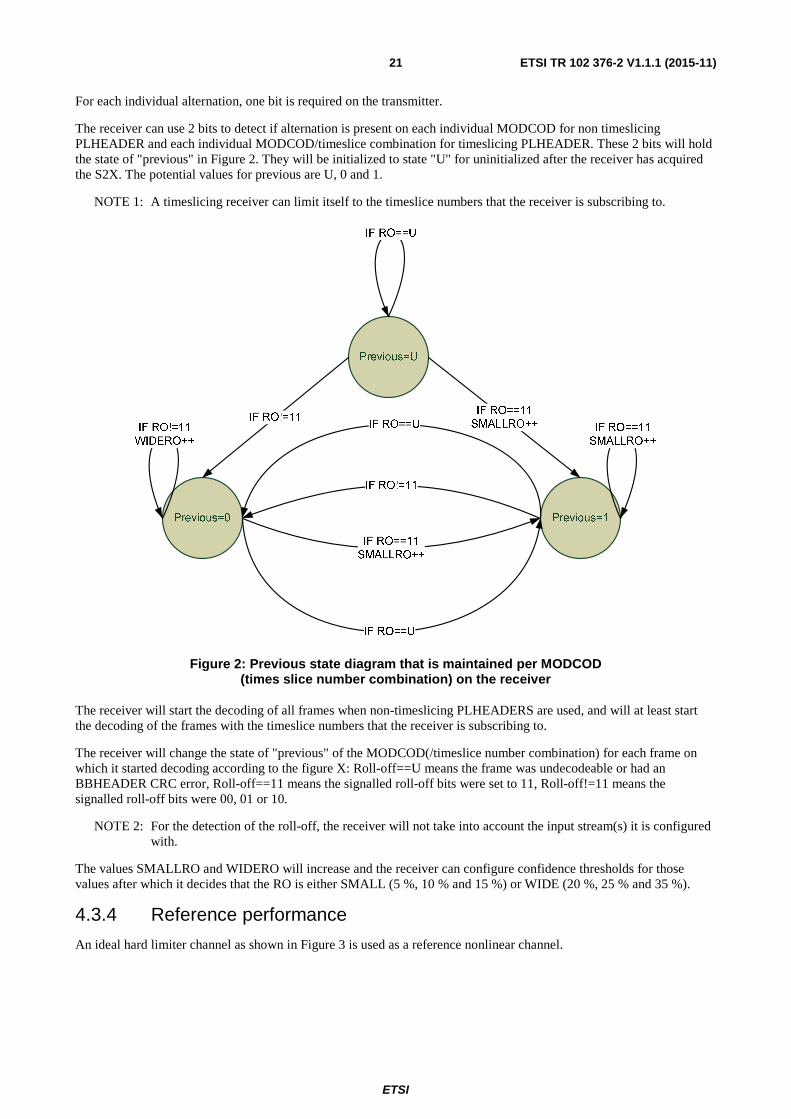
ETSI

ETSI TR 102 376-2 V1.1.1 (2015-11)21

For each individual alternation, one bit is required on the transmitter.

The receiver can use 2 bits to detect if alternation is present on each individual MODCOD for non timeslicing PLHEADER and each individual MODCOD/timeslice combination for timeslicing PLHEADER. These 2 bits will hold the state of "previous" in Figure 2. They will be initialized to state "U" for uninitialized after the receiver has acquired the S2X. The potential values for previous are U, 0 and 1.

NOTE 1: A timeslicing receiver can limit itself to the timeslice numbers that the receiver is subscribing to.

Figure 2: Previous state diagram that is maintained per MODCOD (times slice number combination) on the receiver

The receiver will start the decoding of all frames when non-timeslicing PLHEADERS are used, and will at least start the decoding of the frames with the timeslice numbers that the receiver is subscribing to.

The receiver will change the state of "previous" of the MODCOD(/timeslice number combination) for each frame on which it started decoding according to the figure X: Roll-off==U means the frame was undecodeable or had an BBHEADER CRC error, Roll-off==11 means the signalled roll-off bits were set to 11, Roll-off!=11 means the signalled roll-off bits were 00, 01 or 10.

NOTE 2: For the detection of the roll-off, the receiver will not take into account the input stream(s) it is configured with.

The values SMALLRO and WIDERO will increase and the receiver can configure confidence thresholds for those values after which it decides that the RO is either SMALL (5 %, 10 % and 15 %) or WIDE (20 %, 25 % and 35 %).

4.3.4 Reference performance

An ideal hard limiter channel as shown in Figure 3 is used as a reference nonlinear channel.

ETSI

ETSI TR 102 376-2 V1.1.1 (2015-11)22

Figure 3: Hard limiter TWTA model

Performance of DVB-S2X MODCODs in AWGN and ideal hard limiter channel is shown in Table 1 for the Normal FECFRAME. For the case of hard limiter channel, no transmit or receive nonlinearity compensation is performed, only ring ratios are optimized for constellations with 16 or more symbols.

The spectral efficiency values for 32APSK 2/3-L and 64APSK 5/6 indicated in ETSI EN 302 307-2 v1.1.1 [i.2] are to be disregarded. The values indicated in this Table 1 are to be considered.

Table 2 and Table 3 respectively show the AWGN performance for Medium and Short FECFRAME.

Table 1: Performance at Quasi Error Free FER = 10-5 (see note 5) Normal FECFRAMES, 50 iterations

Canonical MODCOD name

Spectral efficiency [bit/symbol] (see note 4)

Ideal Es/N0 [dB] for (AWGN Linear

Channel) (Normative) (see note 1)

Ideal Csat/(N0⋅Rs) [dB] (Non-Linear Hard Limiter Channel)

(Informative) (see note 2)

Optimized input Back-off

IBO [dB]

(see note 2) QPSK 2/9 0,434841 -2,85 (see note 3) -2,45 -5 QPSK 13/45 0,567805 -2,03 -1,60 -5 QPSK 9/20 0,889135 0,22 0,69 -5 QPSK 11/20 1,088581 1,45 1,97 -5 8APSK 5/9-L 1,647211 4,73 5,95 -3,5 8APSK 26/45-L 1,713601 5,13 6,35 -3,5 8PSK 23/36 1,896173 6,12 6,96 -3,5 8PSK 25/36 2,062148 7,02 7,93 -3,5 8PSK 13/18 2,145136 7,49 8,42 -3,5 16APSK 1/2-L 1,972253 5,97 8,4 0,75 16APSK 8/15-L 2,104850 6,55 9,0 0,25 16APSK 5/9-L 2,193247 6,84 9,35 0,75 16APSK 26/45 2,281645 7,51 9,17 -1,25 16APSK 3/5 2,370043 7,80 9,38 -1,5 16APSK 3/5-L 2,370043 7,41 9,94 2 16APSK 28/45 2,458441 8,10 9,76 -1,5 16APSK 23/36 2,524739 8,38 10,04 -1,25 16APSK 2/3-L 2,635236 8,43 11,06 2 16APSK 25/36 2,745734 9,27 11,04 0,25 16APSK 13/18 2,856231 9,71 11,52 0,25 16APSK 7/9 3,077225 10,65 12,50 0 16APSK 77/90 3,386618 11,99 14,00 0,75 32APSK 2/3-L (see note 6)

3,291954 11,10 13,81 2

32APSK 32/45 3,510192 11,75 14,50 2 32APSK 11/15 3,620536 12,17 14,91 2,25 32APSK 7/9 3,841226 13,05 15,84 2,25 64APSK 32/45-L 4,206428 13,98 17,7 3,5 64APSK 11/15 4,338659 14,81 17,97 2,5 64APSK 7/9 4,603122 15,47 19,10 3,25 64APSK 4/5 4,735354 15,87 19,54 3,25

Pout

Pin

CSAT

0 dB

ETSI

ETSI TR 102 376-2 V1.1.1 (2015-11)23

Canonical MODCOD name

Spectral efficiency [bit/symbol] (see note 4)

Ideal Es/N0 [dB] for (AWGN Linear

Channel) (Normative) (see note 1)

Ideal Csat/(N0⋅Rs) [dB] (Non-Linear Hard Limiter Channel)

(Informative) (see note 2)

Optimized input Back-off

IBO [dB]

(see note 2) 64APSK 5/6 (see note 6)

4,936639 16,55 20,44 3,5

128APSK 3/4 5,163248 17,73 21,43 3,25 128APSK 7/9 5,355556 18,53 22,21 3,25 256APSK 29/45-L 5,065690 16,98 21,6 4,25 256APSK 2/3-L 5,241514 17,24 21,89 4,25 256APSK 31/45-L 5,417338 18,10 22,9 4,5 256APSK 32/45 5,593162 18,59 22,91 4 256APSK 11/15-L 5,768987 18,84 23,80 4,75 256APSK 3/4 5,900855 19,57 24,02 4 NOTE 1: Es is the average energy per transmitted symbol; N0 is the noise power spectral density.

NOTE 2: Csat is the hard limiter pure carrier saturated power; N0⋅Rs is the noise power integrated over a bandwidth equal to the symbol rate. Performance results are for the optimized input back-off (IBO) indicated in the table and for a roll-off = 10 %. Csat/ (N0⋅Rs) is equal to Es,sat/N0 and the difference between the Es/N0 of the AWGN linear channel and Es,sat /N0 is due to the compromise between operating back-off and nonlinear distortion (which is dependent on the roll-off).

NOTE 3: The FECFRAME length is 61 560. NOTE 4: Spectral efficiencies are calculated in a bandwidth equal to the symbol rate Rs in case of no pilots. The

corresponding spectral efficiency for a bandwidth equal to Rs (1 + roll-off) can be computed dividing the numbers in column "spectral efficiency" by (1 + roll-off).

NOTE 5: Note that in ETSI EN 302 307-1 [i.1], Table 13, performance was defined for Quasi Error Free PER = 10-7, wherein a packet is defined to have 188 bytes. It can be assumed that performance at PER = 10-7 is comparable to that at FER = 10-5.

NOTE 6: The modcods 32APSK 2/3-L and 64APSK 5/6 use the DVB-S2 LDPC codes. As a result, the corresponding BCH codes for these two modcods have t = 10.

NOTE 7: The spectral efficiency in case of no pilots is given by η = (kBCH-80) / [90 (S + 1)], where kBCH is the number of bits of BCH uncoded Block and S is the number of SLOTs (of size M = 90 symbols) per XFECFRAME. When pilots are present, the spectral efficiency can be computed as η = (kBCH-80) / [90 (S + 1) + P int{(S-1) / 16}], where P = 36 is the length of the pilot sequence and int{.} is the integer function.

The spectral efficiency values for 32APSK 2/3-L and 64APSK 5/6 indicated in ETSI EN 302 307-2 v1.1.1 [i.2] are to be disregarded. The values indicated in this Table 1 are to be considered.

Table 2: Es/N0 Performance at Quasi Error Free FER = 10-5 (AWGN Channel) medium XFECFRAMEs, 75 iterations

Canonical MODCOD name Ideal Es/N0 (dB) for FECFRAME length = 30 780

BPSK 1/5 -6,85 BPSK 11/45 -5,50

BPSK 1/3 -4,00

ETSI

ETSI TR 102 376-2 V1.1.1 (2015-11)24

Table 3: Es/N0 Performance at Quasi Error Free FER = 10-5 (AWGN Channel) Short XFECFRAMEs, 75 iterations π/2 BPSK modes, 50 iterations other modes

Canonical MODCOD name Ideal Es/N0 (dB) for FECFRAME length = 16 200

BPSK-S 1/5 -9,9 (note 1) BPSK-S 11/45 -8,3 (note 1)

BPSK 1/5 -6,1 (note 2) BPSK 4/15 -4,9 (note 2) BPSK 1/3 -3,72

QPSK 11/45 -2,50 QPSK 4/15 -2,24

QPSK 14/45 -1,46 QPSK 7/15 0,60 QPSK 8/15 1,45

QPSK 32/45 3,66 8PSK 7/15 3,83 8PSK 8/15 4,71

8PSK 26/45 5,52 8PSK 32/45 7,54

16APSK 7/15 5,99 16APSK 8/15 6,93

16APSK 26/45 7,66 16APSK 3/5 8,10

16APSK 32/45 9,81 32APSK 2/3 11,41

32APSK 32/45 12,18 NOTE 1: The FECFRAME length is 15 390. NOTE 2: The FECFRAME length is 14 976.

4.4 Channel models

4.4.0 Introduction

The scope of this clause is to define suitable channel models for performance evaluation of DVB-S2X in the various application areas.

The following services, divided in "core markets" and "emerging markets", are addressed within the scope of the present document:

• Core markets: Direct-To-Home, broadcast distribution, contribution, VSAT outbound and high speed IP links.

• Emerging markets: airborne, rail and other mobile forward links, small aperture terminals for news gathering, disaster relief and similar ad hoc links, and VSAT forward links in regions prone to deep transient atmospheric fading.

It is to be underlined that it is not the scope of the clause to thoroughly represent all the possible scenarios for the considered set of services. Instead, a limited set of channel models are selected if deemed to contribute in specific performance differentiation of the proposed physical layer techniques for DVB-S2X.

Also to be remarked that the specific satellite transponder characteristics that have been used in the present document are not meant to be considered as reference design for broadcast and broadband satellite payloads supporting next generation DVB-S2X specifications. It is recognized that the detailed specifications and characteristics of these transponders may present relatively large variations depending on many different design criteria. In the present document, instead, a rather limited set of characteristics for legacy sub-systems has been chosen in order to be able to test new techniques within a limited computer simulation effort.

ETSI

ETSI TR 102 376-2 V1.1.1 (2015-11)25

4.4.1 DTH Broadcasting services

4.4.1.0 General description

For DTH broadcasting services, both Ku and Ka bands will be considered. Although it is recognized that DTH service can also be provided in multi-carrier per TWTA configuration, in the following will be focused on single carrier per transponder operations.

Although uplink of multiple carriers from a single station is also possible, here three carriers are considered uplinked by three different ground stations, geographically separated. The carrier frequencies are equal to the transponder center frequencies. Within this set, the carrier under test is assumed to be the central frequency carrier (i.e. the one with two adjacent carriers on each side). The adjacent carriers are simulated from the carrier under test by delaying the latter by different time delays so as to simulate complete uncorrelation among the carriers. It is recommended to set these values to multiple of 50,2 symbols (see note 1) in order to:

1) ensure uncorrelation among the carriers even when considering transmit shaping filters with very long tails in time; and

2) to avoid perfect symbol timing synchronization. Following this recommendation, the set of delays is to be fixed as follows:

DELAY5 = 50,2 symbols, DELAY6 = 100,4 symbols.

The carrier under test (central carrier) is also optionally reduced in power by a factor APU to take into account any uncompensated fading events on the uplink: the proposed set-up assumes that the two adjacent carriers do not suffer from fading while the central carrier is possibly subject of fading of up to 8 dB. This represents a worst case condition in that:

i) the two adjacent carriers are assumed in clear sky (worst case uplink interference); and

ii) the ground stations are assumed to be without up-link power control.

The AM/AM and AM/PM characteristics of the HPA of the three uplink stations are simulated by the model described in Figure 5. As for the operating point of the HPA (assumed the same for the three stations), an optimized value has to be selected also taking into account the requirement to minimize the adjacent channel interference. It is important to underline that, in order to well represent the non-linear behaviour of the HPA, a high sampling frequency has to be used, so as to avoid aliasing effects of the intermodulation distortion images. A minimum oversampling factor of 10 (with respect to the composite - i.e. of the set of carriers - signal bandwidth) is recommended.

Following the HPA, the IMUX filter selects the carrier under test and remove the other adjacent carriers, following the transfer function model of Figure 6.

The second block of the transponder corresponds to the TWTA for which two models exist for the AM/AM and AM/PM characteristics, i.e. the conventional model of Figure 10 and the linearized model of Figure 11. The single carrier that has been selected by the IMUX is amplified at an operating point to be optimized. Same considerations as in the case of the ground station HPA applies here for what concerns the requirements for the oversampling factor.

Next, the OMUX filter is responsible for shaping the non-linearly distorted carrier in order to limit the interference to adjacent transponders. Its frequency response model is depicted in Figure 7. The next block introduces in the channel the effects of the adjacent transponder interference, by shifting in time and frequency the carrier under test so as to simulate the adjacent transponder carriers placed and ±fT and at the same power level (see note 2). The delays of the models have to be selected with criteria which are very similar to the ones used for the ground station adjacent carriers. It is then suggested to use DELAY1 = 75,2 symbols and DELAY2 = 125,4 symbols.

The model does not take into account that in the reality the adjacent transponder interference signal that occurs before the transponder and the one that occurs after the transponder are correlated. Therefore, the total power is higher than sum of powers. The impact on the performance can however be considered very low.

Cross-polar interference is then added to the channel according to the models described in clauses 4.4.1.3 and 4.4.1.5. In particular, the amplitudes Ap1, Ap2 and the frequencies fp1 and fp2 should be selected according to Table 5. DELAY3 and DELAY4 are set to 25,6 symbols and 100,8 symbols.

ETSI

ETSI TR 102 376-2 V1.1.1 (2015-11)26

The blocks labelled in red "Adjacent Satellite Interference" can be optionally included. For advanced techniques which aims at mitigating its impact to the end-to-end performance, its model is described in clause 4.4.1.5.1, otherwise it is assumed that the adjacent satellite interference is modelled through an additional white Gaussian noise with a C/IADJ of 14 dB.

NOTE 1: These delays can also be expressed as function of the inverse of the signal bandwidth (which should coarsely match the one of the IMUX filter). This approach would better respond to the requirements of modulations where the length of the signalling pulse is more directly related to the signal bandwidth as opposed to the symbol rate.

NOTE 2: Although it is recognized that is some cases the output power of adjacent transponders may differ by 1 or 2 dB maximum due to a possible different OBO setting.

The AWGN block adds the noise to the channel according to the target signal to noise ratio. The terminal receiver imperfections are then added through the phase and frequency errors mainly caused by the LNB (see clause 4.4.1.6 for the details of the model) and the amplitude gain ripple and slope caused by the LNB and the interfacility link coax cable (see clause 4.4.1.7).

*: To be modelled if the bandwidth of the signal carrier is greater than the nominal transponder bandwidth. **: To be modelled according to the models of Figure 12 and Figure 13. ***: To be modelled as an additional AWGN or if adjacent satellite interference cancellation techniques are

considered, according to Figure 15.

Figure 4: Channel model Block diagram for the DTH broadcasting services

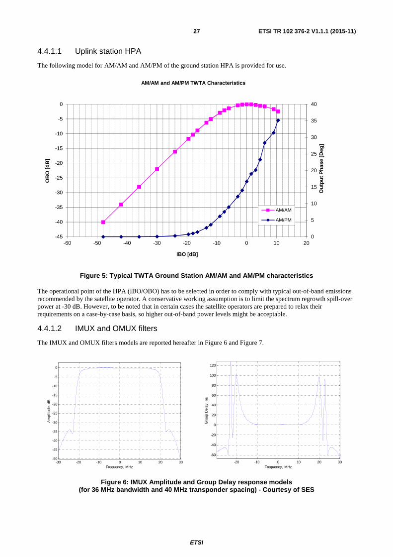
ETSI

ETSI TR 102 376-2 V1.1.1 (2015-11)27

4.4.1.1 Uplink station HPA

The following model for AM/AM and AM/PM of the ground station HPA is provided for use.

Figure 5: Typical TWTA Ground Station AM/AM and AM/PM characteristics

The operational point of the HPA (IBO/OBO) has to be selected in order to comply with typical out-of-band emissions recommended by the satellite operator. A conservative working assumption is to limit the spectrum regrowth spill-over power at -30 dB. However, to be noted that in certain cases the satellite operators are prepared to relax their requirements on a case-by-case basis, so higher out-of-band power levels might be acceptable.

4.4.1.2 IMUX and OMUX filters

The IMUX and OMUX filters models are reported hereafter in Figure 6 and Figure 7.

Figure 6: IMUX Amplitude and Group Delay response models (for 36 MHz bandwidth and 40 MHz transponder spacing) - Courtesy of SES

0

5

10

15

20

25

30

35

40

-45

-40

-35

-30

-25

-20

-15

-10

-5

0

-60 -50 -40 -30 -20 -10 0 10 20

Ou

tpu

t P

has

e [D

eg]

OB

O [

dB

]

IBO [dB]

AM/AM and AM/PM TWTA Characteristics

AM/AM

AM/PM

-30 -20 -10 0 10 20 30-50

-45

-40

-35

-30

-25

-20

-15

-10

-5

0

Frequency, MHz

Am

plitu

de,

dB

-20 -10 0 10 20 30

-60

-40

-20

0

20

40

60

80

100

120

Frequency, MHz

Gro

up D

elay

, ns

ETSI

ETSI TR 102 376-2 V1.1.1 (2015-11)28

Figure 7: OMUX Amplitude and Group Delay response model (for 36 MHz bandwidth and 40 MHz transponder spacing) - Courtesy of SES

The amplitude and group delay numerical entries for these filters are provided in the embedded text files of annex E, where the 26 MHz and 33 MHz versions are also present.

In clause H.7 of ETSI EN 302 307-1 [i.1] the following scaling formula is suggested for using the same frequency responses at a different transponder bandwidth:

R(f) = Rejection (f x 36/BW(MHz))

G(f) = (36/BW(MHz)) × Group-delay (f x 36/BW(MHz))

This assumes also that the ratio between the transponders' spacing and the transponder bandwidth remains constant at a value equal to 40/36 = 1,11.

It is recognized that these scaling formulas cannot exactly reproduce the exact frequency response for any bandwidth, while instead they can produce a fairly good approximation, at least for the purpose of estimating the end-to-end link performance.

These filters, though being taken from a real transponder, are not meant to exactly model the transfer function of all the OMUX and IMUX filters being deployed in existing payloads, as a relatively large variation of characteristics may occur (in particular also the ratio between transponder spacing and bandwidth do vary). Nevertheless, these models are considered quite common in existing broadcast payloads.

The IMUX/OMUX transfer function define the transponder bandwidth. In the present document the following naming convention will be used:

• Nominal transponder bandwidth: is the transponder bandwidth where the amplitude response of the IMUX/OMUX filters is "almost flat". This corresponds to 36 MHz for the filters in Figure 6 and Figure 7.

• Transponder Frequency spacing, is the distance of center frequency of adjacent transponders. For example, for 36 MHz transponders a spacing of 40 MHz may be used. Throughout the present document it will be assumed that for any nominal transponder/beam bandwidth, the spacing is set to 40/36 = 1,11 times the nominal bandwidth.

The following cases are used as references:

1) 36 MHz IMUX and OMUX filters with a spacing of 40 MHz.

2) 225 MHz IMUX and OMUX filters (in the scaling formula of clause 4.4.1.2 replace BW with 225) with a spacing of 250 MHz.

-30 -20 -10 0 10 20 30

-50

-45

-40

-35

-30

-25

-20

-15

-10

-5

0

Frequency, MHz

Am

plitu

de,

dB

-30 -20 -10 0 10 20 30

-30

-20

-10

0

10

20

30

40

50

Frequency, MHz

Gro

up D

elay

, ns

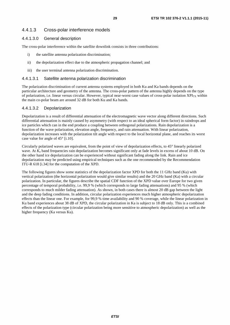
ETSI

ETSI TR 102 376-2 V1.1.1 (2015-11)29

4.4.1.3 Cross-polar interference models

4.4.1.3.0 General description

The cross-polar interference within the satellite downlink consists in three contributions:

i) the satellite antenna polarization discrimination;

ii) the depolarization effect due to the atmospheric propagation channel; and

iii) the user terminal antenna polarization discrimination.

4.4.1.3.1 Satellite antenna polarization discrimination

The polarization discrimination of current antenna systems employed in both Ku and Ka bands depends on the particular architecture and geometry of the antenna. The cross-polar pattern of the antenna highly depends on the type of polarization, i.e. linear versus circular. However, typical near-worst case values of cross-polar isolation XPITX within the main co-polar beam are around 32 dB for both Ku and Ka bands.

4.4.1.3.2 Depolarization

Depolarization is a result of differential attenuation of the electromagnetic wave vector along different directions. Such differential attenuation is mainly caused by asymmetry (with respect to an ideal spherical form factor) in raindrops and ice particles which can in the end produce a coupling between orthogonal polarizations. Rain depolarization is a function of the wave polarization, elevation angle, frequency, and rain attenuation. With linear polarization, depolarization increases with the polarization tilt angle with respect to the local horizontal plane, and reaches its worst case value for angle of 45° [i.10].

Circularly polarized waves are equivalent, from the point of view of depolarization effects, to 45° linearly polarized wave. At Ka band frequencies rain depolarization becomes significant only at fade levels in excess of about 10 dB. On the other hand ice depolarization can be experienced without significant fading along the link. Rain and ice depolarization may be predicted using empirical techniques such as the one recommended by the Recommendation ITU-R 618 [i.34] for the computation of the XPD.

The following figures show some statistics of the depolarization factor XPD for both the 11 GHz band (Ku) with vertical polarization (the horizontal polarization would give similar results) and the 20 GHz band (Ka) with a circular polarization. In particular, the figures describe the spatial CDF function of the XPD value over Europe for two given percentage of temporal probability, i.e. 99,9 % (which corresponds to large fading attenuations) and 95 % (which corresponds to much milder fading attenuation). As shown, in both cases there is almost 20 dB gap between the light and the deep fading conditions. In addition, circular polarization experiences much higher atmospheric depolarization effects than the linear one. For example, for 99,9 % time availability and 90 % coverage, while the linear polarization in Ku band experiences about 38 dB of XPD, the circular polarization in Ka is subject to 18 dB only. This is a combined effects of the polarization type (circular polarization being more sensitive to atmospheric depolarization) as well as the higher frequency (Ka versus Ku).

ETSI

ETSI TR 102 376-2 V1.1.1 (2015-11)30

Figure 8: Cumulative Distribution Function of the atmospheric depolarization XPD in Ku band and vertical linear polarization

Figure 9: Cumulative Distribution Function of the atmospheric depolarization XPD in Ku band and vertical polarization

4.4.1.3.3 User terminal outdoor unit polarization isolation

Typical value near worst case values XPIRX are in the range 20 to 25 dB for both Ku and Ka bands and linear and circular polarizations. In the simulations the XPIRX was set to 25 dB.

ETSI

ETSI TR 102 376-2 V1.1.1 (2015-11)31

4.4.1.3.4 Cross-polarization summary model

The total cross-polar interference power can be computed by adding the interference power contributions from the three components described above:

Icross = IcrossTX + Icross

RX + Idepol

Under the assumption of equal transmitted power in both polarization, it can be shown that the total C/I due to cross-polar interference can be computed as:

C/Icross = [ XPITX-1 + XPIRX

-1 + XPD-1]-1

Considering only the XPI terms (satellite and terminal antenna) the total is around 24 dB so the XPD contribution may be considered negligible at Ku band with linear polarization (XPD being higher than 38 dB), while at Ka-band with circular polarization the total C/I would result to about 17dB when in the presence of deep fading events, while it would be similar to the Ku-band case (24 dB) for light fading attenuations. This is all summarized in Table 4.

Table 4: Near-worst case ( in time and location) Carrier-to-Interference ratio values for two scenarios over Europe

Ku band - Linear Polarization C/Icross, dB

Ka band - Circular Polarization C/Icross, dB

24 Deep fading: 17 Light fading: 24

4.4.1.4 On-board TWTA

The following conventional and linearized TWTA AM/AM and AM/PM characteristics is provided to be used to test the end-to-end performance for all the conceivable transponder bandwidths both in Ku and Ka bands. Single carrier per transponder operation is assumed.

Figure 10: Conventional TWTA Amplitude and Phase response model as in ETSI EN 302 307-1 [i.1]

-10

0

10

20

30

40

50

60

70

-16

-14

-12

-10

-8

-6

-4

-2

0

-20 -18 -16 -14 -12 -10 -8 -6 -4 -2 0 2 4 6

Ou

tpu

t P

has

e [D

eg]

OU

TP

UT

PO

WE

R [d

B]

INPUT POWER [dB]

Ka-band TWTA - Single Carrier Transfer Characteristics

OUTPUT POWER

PHASE

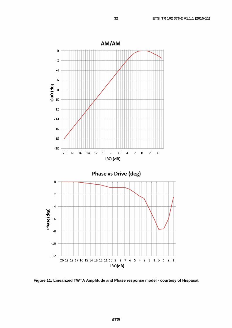
ETSI

ETSI TR 102 376-2 V1.1.1 (2015-11)32

Figure 11: Linearized TWTA Amplitude and Phase response model - courtesy of Hispasat

-20

-18

-16

-14

-12

-10

-8

-6

-4

-2

0

-20 -18 -16 -14 -12 -10 -8 -6 -4 -2 0 2 4

OBO (dB)

IBO (dB)

AM/AM

-12

-10

-8

-6

-4

-2

0

-20-19-18-17-16-15-14-13-12-11-10 -9 -8 -7 -6 -5 -4 -3 -2 -1 0 1 2 3

Phase (deg)

IBO(dB)

Phase vs Drive (deg)

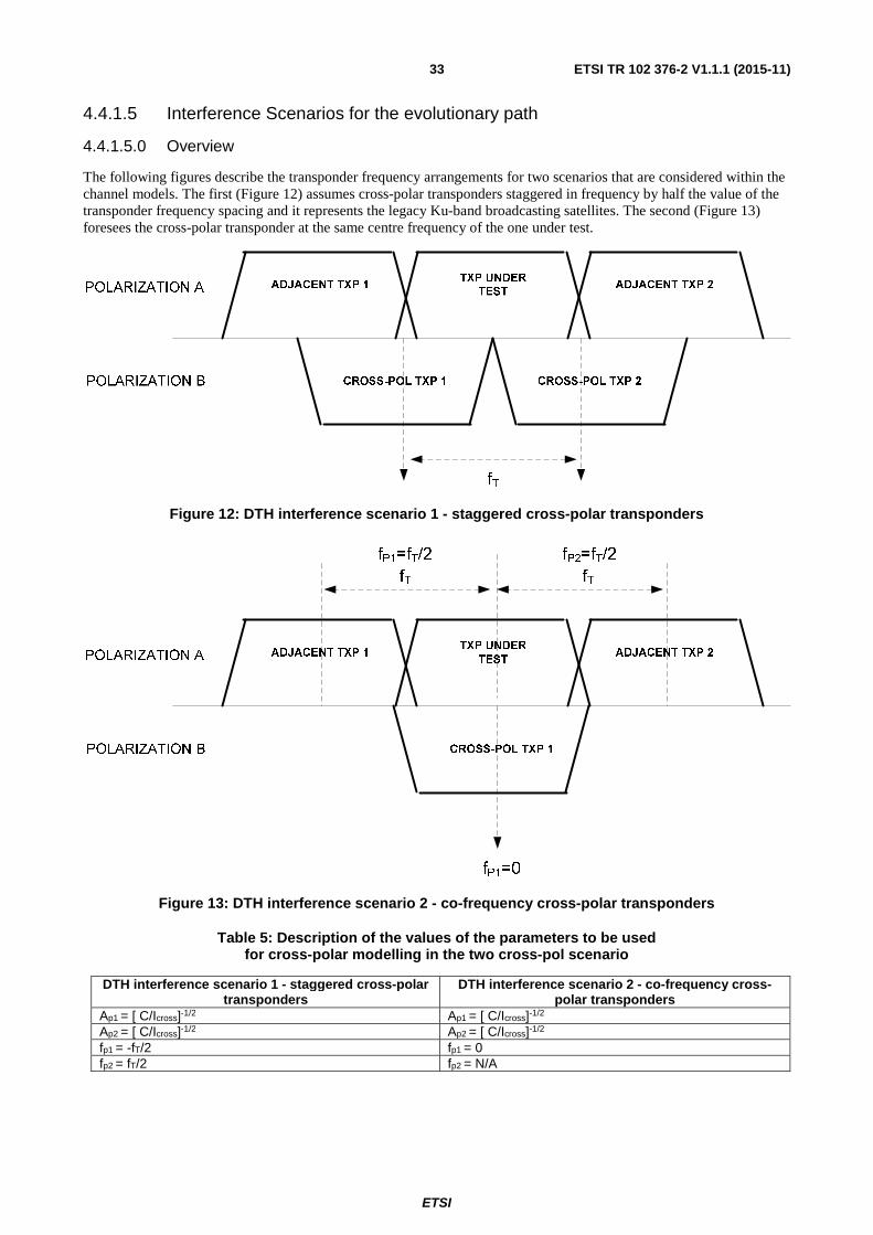
ETSI

ETSI TR 102 376-2 V1.1.1 (2015-11)33

4.4.1.5 Interference Scenarios for the evolutionary path

4.4.1.5.0 Overview

The following figures describe the transponder frequency arrangements for two scenarios that are considered within the channel models. The first (Figure 12) assumes cross-polar transponders staggered in frequency by half the value of the transponder frequency spacing and it represents the legacy Ku-band broadcasting satellites. The second (Figure 13) foresees the cross-polar transponder at the same centre frequency of the one under test.

Figure 12: DTH interference scenario 1 - staggered cross-polar transponders

Figure 13: DTH interference scenario 2 - co-frequency cross-polar transponders

Table 5: Description of the values of the parameters to be used for cross-polar modelling in the two cross-pol scenario

DTH interference scenario 1 - staggered cross-polar transponders

DTH interference scenario 2 - co-frequency cross-polar transponders

Ap1 = [ C/Icross]-1/2 Ap1 = [ C/Icross]-1/2 Ap2 = [ C/Icross]-1/2 Ap2 = [ C/Icross]-1/2 fp1 = -fT/2 fp1 = 0 fp2 = fT/2 fp2 = N/A

fP1=fT/2 fP2=fT/2

POLARIZATION A

POLARIZATION B

fT fT

fP1=0

TXP UNDER

TESTADJACENT TXP 1 ADJACENT TXP 2

CROSS-POL TXP 1

ETSI

ETSI TR 102 376-2 V1.1.1 (2015-11)34

4.4.1.5.1 Adjacent Satellite Interference

In addition to the interference scenarios depicted in the previous clause, the adjacent satellite interference may also be modelled following reference [i.6].

We will assume a realistic broadcast satellite constellation around the geostationary arc, the orbital spacing as seen from a typical position in the middle of Europe is summarized in Table 6.

Table 6: Orbital spacing as seen from a typical position in the middle of Europe

Sat 7 Sat 5 Sat 3 Sat 1 Sat 2 Sat 4 Sat 6 Sat 8 -9,2° -6,2° -3,2° 0° +2,4° +4,3° +6,8° +9,0°

The realistic interference situation is difficult to be reflected in general terms, because it involves International Telecommunication Union (ITU) established limits as well as specific confidential bilateral agreements among satellite operators, which can change from one frequency band to another. However, it is very reasonable to assume that most of that interference limited scenarios involve a small number of interferers. In the following, equal power density limits on the different satellite positions is assumed. The following figure illustrates the signal to noise and the signal to interference ratio for different aperture sizes. The aggregate interference is assumed to be at its maximum "worst-case" level according to existing common ITU regulatory limitations. We further assume that the desired signal is received from satellite Sat 1 and the dominating interference is attributed to Sat 2. Fading due to rain (at the target availability) is also taken into account and affects all signals.

Figure 14: Plot of the signal-to-noise (C/N), interference (C/I) and combined C/(N+I) ratios as a function of the antenna aperture (assuming parabolic reflectors)

From Figure 14 it can be seen that for a typical receiver antenna aperture size between 50 and 60 cm, the C/IADJ varies between 12 and 16 dB.

If no interference mitigation techniques is assumed at the receiver, this interference can be modelled as an additional AWGN with the mentioned C/IADJ. If one value is to be chosen, a C/IADJ of 14 dB can be considered as a realistic interference level in a number of practical broadcast reception systems.

NOTE: In this scenario the combination of narrow orbital spacing and equal power density limits causes low C/I_adj This scenario is used in simulations as a challenging case. The actual scenario in Europe is characterized by satellite positions with high and low power density alternately, which facilitates receiving the high power density positions with small antennas.

-4.0

-3.0

-2.0

-1.0

0.0

1.0

2.0

3.0

4.0

5.0

6.0

7.0

8.0

9.0

10.0

11.0

12.0

13.0

14.0

15.0

16.0

17.0

18.0

0 0.1 0.2 0.3 0.4 0.5 0.6 0.7

ASI, C/N, C/(N+I) [dB]

Reception antenna aperture [m]

Adjacent Satellite Interference Impact - Example Broadcast Reception Scenario

C/N DL

ASI [dB]

C/(N+I) [dB]

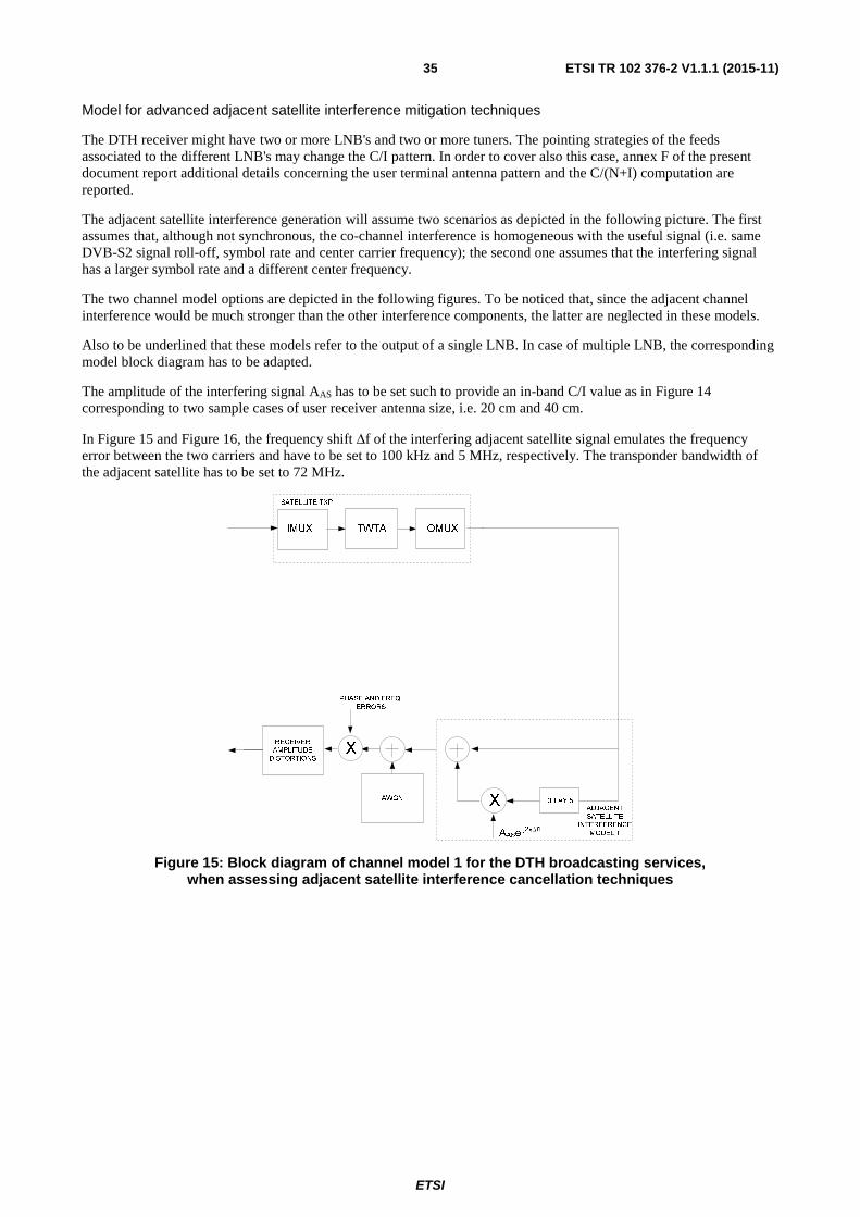
ETSI

ETSI TR 102 376-2 V1.1.1 (2015-11)35

Model for advanced adjacent satellite interference mitigation techniques

The DTH receiver might have two or more LNB's and two or more tuners. The pointing strategies of the feeds associated to the different LNB's may change the C/I pattern. In order to cover also this case, annex F of the present document report additional details concerning the user terminal antenna pattern and the C/(N+I) computation are reported.

The adjacent satellite interference generation will assume two scenarios as depicted in the following picture. The first assumes that, although not synchronous, the co-channel interference is homogeneous with the useful signal (i.e. same DVB-S2 signal roll-off, symbol rate and center carrier frequency); the second one assumes that the interfering signal has a larger symbol rate and a different center frequency.

The two channel model options are depicted in the following figures. To be noticed that, since the adjacent channel interference would be much stronger than the other interference components, the latter are neglected in these models.

Also to be underlined that these models refer to the output of a single LNB. In case of multiple LNB, the corresponding model block diagram has to be adapted.

The amplitude of the interfering signal AAS has to be set such to provide an in-band C/I value as in Figure 14 corresponding to two sample cases of user receiver antenna size, i.e. 20 cm and 40 cm.

In Figure 15 and Figure 16, the frequency shift Δf of the interfering adjacent satellite signal emulates the frequency error between the two carriers and have to be set to 100 kHz and 5 MHz, respectively. The transponder bandwidth of the adjacent satellite has to be set to 72 MHz.

Figure 15: Block diagram of channel model 1 for the DTH broadcasting services, when assessing adjacent satellite interference cancellation techniques

SATELLITE TXP

IMUX TWTA OMUX

RECEIVER

AMPLITUDE

DISTORTIONS

AWGN

X

PHASE AND FREQ.

ERRORS

DELAY 5X

AASe-j2 ft

ADJACENT

SATELLITE

INTERFERENCE

MODEL 1

ETSI

ETSI TR 102 376-2 V1.1.1 (2015-11)36

Figure 16: Block diagram of channel model 2 for the DTH broadcasting services, when assessing adjacent satellite interference cancellation techniques

4.4.1.6 Phase and Frequency Errors

4.4.1.6.1 Phase noise

A number of DTH phase noise masks are proposed according to the band (Ku and Ka) and the state of the art (2012) and older equipments (2000). The contributions from the hub (uplink), the satellite payload as well as the receiver (downlink) have been taken into account.

Table 7: Phase noise masks proposed for the DTH services

Offset (Hz)

PROFILE "2000-Ku- DTH" SSB (dBc/Hz)

uplink satellite downlink tot-

equiv 10

100 -60 -62 -25 -25,00 1 K -70 -81 -50 -50,00 10 K -80 -84 -73 -72,90

100 K -90 -94 -85 -84,76 1 M -90 -94 -103 -89,68

10 M -90 -94 -114 -89,68

Offset (Hz)

PROFILE "2012-Ka- DTH" SSB (dBc/Hz)

uplink satellite downlink tot-

equiv 10

100 -72 -62 -25 -25,00 1 K -82 -80 -50 -50,00 10 K -92 -90 -73 -73,00

100 K -102 -95 -93 -92,25 1 M -112 -106 -103 -102,49

10 M -122 -116 -114 -113,23 50 M -124 -118 -117 -115,89

ETSI

ETSI TR 102 376-2 V1.1.1 (2015-11)37

Figure 17: Phase noise power spectral density masks for the DTH service

In order to limit the number of phase noise masks to be used, a proposal is to mandate the "Ka 2012" mask as first priority and the "Ku 2000" as second priority but only for symbol rates lower than 36 Mbaud (which is most likely the highest conceivable symbol rate through a 36 MHz transponder - 40 MHz spacing).

In summary, the two phase noise masks to be used are:

Table 8: Phase noise masks to be used for the DTH broadcasting services

Masks 100 Hz 1 kHz 10 kHz 100 kHz 1 MHz 10 MHz ≥ 50 MHz P1 mask SSB dBc/Hz

-25 -50 -73 -92,25 -102,49 -113,23 -115,89

P2 symbol rates less than 36 Mbaud SSB dBc/Hz

-25 -50 -72,90 -84,76 -89,68 -89,68 -89,68

The introduction of the phase noise in the channel mask requires defining an absolute value of transponder frequency spacing for assessing the impact of phase noise to the end to end link performance. For this purpose, the cases outlined in clause 4.4.1.2 can be used as references.

Offset

(Hz)

uplink satellite downlink tot-equiv

10

100 -72 -62 -28 -28.00

1K -82 -81 -53 -53.00

10K -92 -91 -76 -76.00

100K -102 -100 -96 -95.57

1M -112 -110 -106 -105.57

10M -122 -120 -117 -116.35

50M -124 -121 -120 -118.74

PROFILE "2012-Ku- DTH"

SSB (dBc/Hz)

102

103

104

105

106

107

108

-120

-110

-100

-90

-80

-70

-60

-50

-40

-30

-20

Frequency, Hz

SS

B P

SD

, dB

c/H

z

EN302307 typicalEN302307 criticalTM-S20102 Ku 2000TM-S20102 Ku 2012TM-S20102 Ka 2012

ETSI

ETSI TR 102 376-2 V1.1.1 (2015-11)38

For information purposes, annex H describes a methodology that can be used to model the phase noise contribution within computer simulations.

4.4.1.6.2 Carrier Frequency instabilities

As described in ETSI TR 102 376-1 [i.3], the max carrier frequency instability, mainly due to the LNB, is ±5 MHz. However, when tuning to a specific carrier, a more limited frequency errors can be assumed., i.e. ±100 kHz. In addition, in very low cost equipments, the LNB carrier frequency, in certain conditions, (i.e. when illuminated by the sun) may be subject to a time-varying frequency error with a slope of 30 KHz/s. The demodulator has to have the capability to stay lock in the presence of such frequency ramp.

4.4.1.7 Receiver Amplitude Distortions

The receiver ODU LNB and the interfacility link cable are responsible for introducing some frequency selective amplitude distortions to the received signal. The LNB in particular represents a source of both gain ripple and slope. The coax cable in turns introduces a gain slope which is proportional to its length. Often, the LNB frequency response is such to compensate the negative gain slope caused by a "worst case length" coax cable. Depending on the model of the LNB and the length and quality of the cable, the residual gain slope vary quite significantly. In the following, it will be assumed that this variation is equivalent to ±2 dB over 500 MHz band.

Figure 18: Channel model for the DTH terminal amplitude gain ripple and slope

The Δ function can be modelled as a sine wave with 1,5 dB amplitude peak-to-peak and a period of 50 MHz.

4.4.1.8 Fading Dynamics

For DTH reception in Ku band, the typical satellite EIRP varies between 47 and 63 dBW. Different terminal antenna sizes are requested to support DTH reception, according to the geographical position of the user within the satellite coverage. The C/N ranges supported by the MODCODS in ETSI EN 302 307-1 [i.1] are deemed to be well in line with the typical link budget.

For Ka-band, the following figure shows the link budget results for a 45 cm user antenna with wide transponders (208 Mbaud carrier) in three different locations in Europe and North America. The corresponding fading attenuation values at 99,9 % availability are listed in Table 9.

ETSI

ETSI TR 102 376-2 V1.1.1 (2015-11)39

Figure 18a: C/N values as function of EIRP for DTH services at Ka-band

Table 9: Fading attenuation at Ka band for the selected cities

City Lyon Atlanta Milan Fading attenuation

at 99,9 % availability 6,4 dB 11 dB 7,8 dB

In Figure 18a the EIRP value corresponding to 1 meter satellite antenna aperture and 130 W RF saturated power has been highlighted as corresponding to wide regional spot beam coverage and state of the art TWTA's in Ka-band.

4.4.2 VSAT Outbound

4.4.2.1 Scenarios

4.4.2.1.1 Single Beam in Ku-band

For the single beam Ku-band scenario the channel model can be considered equivalent to the one described in clause 4.1.1.1 for the broadcasting services with single carrier per HPA operations. The only deviations to that model (which also apply to the Ka-band scenarios outlined in the next clause) is detailed in the following:

• The phase noise of clause 4.4.1.6.1 does not apply due to the better characteristics of the receiver terminal ODU oscillator. Instead, the phase noise mask to be used are the ones described in clause 4.4.2.4.

• For the same reasons of the previous point, the carrier frequency instabilities are to be set to ±3 MHz. No frequency ramp model has to be assumed due to sun illumination of the ODU.

• For the revolutionary path, the usage of very small dish sizes may be addressed but with an additional justification pertaining the assessment of adjacent satellite interference in the return link.

4.4.2.1.2 Multi-spot beam in Ka-band

4.4.2.1.2.0 General description of the scenarios

A number of scenarios of multi-spot beam networks in Ka-band have been considered, with the objectives of determining the ranges of the main link performance parameters like C/N and C/I. A more detailed characterization of the intra-system co-channel interference is a useful outcome when this constitutes the most performance limiting factor. However, the variability of specific system configurations depending on the satellite platform, coverage and the assumed payload technology is such that the resulting C/N and C/I performance may significantly differ.

52 54 56 58 60 62 64 66 68 70 72-15

-10

-5

0

5

10

15

Satellite EIRP/carrier , dBW

Car

rier

C/N

, dB

Lyon and satellite at 13 degAtlanta and satellite at -80 degMilan and satellite at 13 deg

DTH receiver dish diameter = 45 cm Frequency = 20 GHz Carrier symbol rate = 208 Mbaud Availability = 99.9%

1 m satellite antenna diameter130 W RF power

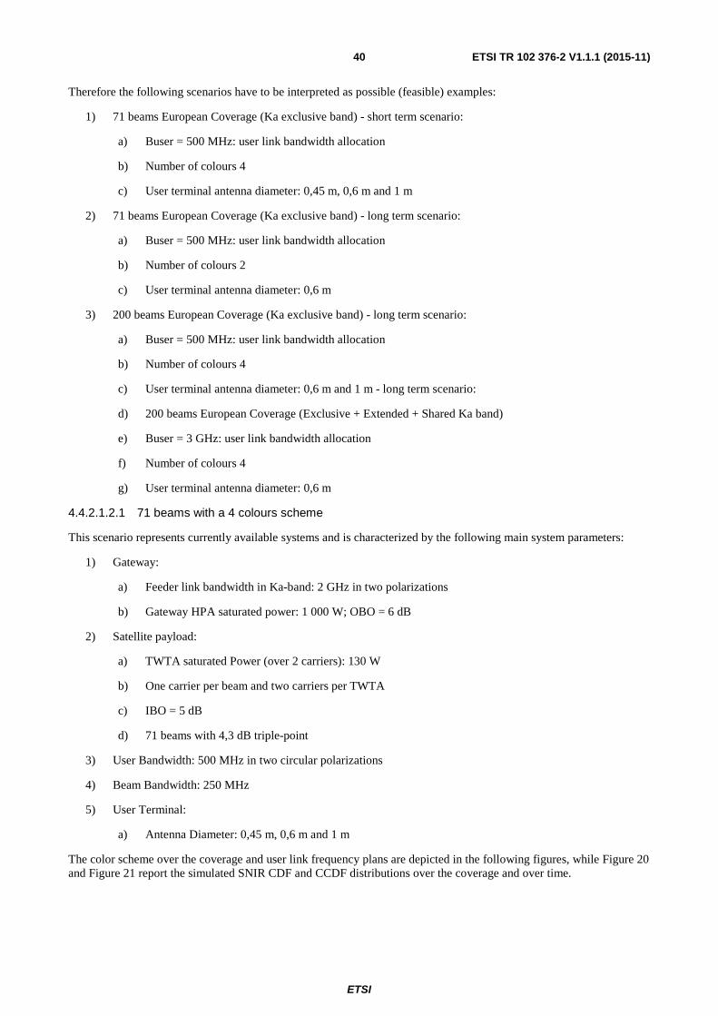
ETSI

ETSI TR 102 376-2 V1.1.1 (2015-11)40

Therefore the following scenarios have to be interpreted as possible (feasible) examples:

1) 71 beams European Coverage (Ka exclusive band) - short term scenario:

a) Buser = 500 MHz: user link bandwidth allocation

b) Number of colours 4

c) User terminal antenna diameter: 0,45 m, 0,6 m and 1 m

2) 71 beams European Coverage (Ka exclusive band) - long term scenario:

a) Buser = 500 MHz: user link bandwidth allocation

b) Number of colours 2

c) User terminal antenna diameter: 0,6 m

3) 200 beams European Coverage (Ka exclusive band) - long term scenario:

a) Buser = 500 MHz: user link bandwidth allocation

b) Number of colours 4

c) User terminal antenna diameter: 0,6 m and 1 m - long term scenario:

d) 200 beams European Coverage (Exclusive + Extended + Shared Ka band)

e) Buser = 3 GHz: user link bandwidth allocation

f) Number of colours 4

g) User terminal antenna diameter: 0,6 m

4.4.2.1.2.1 71 beams with a 4 colours scheme

This scenario represents currently available systems and is characterized by the following main system parameters:

1) Gateway:

a) Feeder link bandwidth in Ka-band: 2 GHz in two polarizations

b) Gateway HPA saturated power: 1 000 W; OBO = 6 dB

2) Satellite payload:

a) TWTA saturated Power (over 2 carriers): 130 W

b) One carrier per beam and two carriers per TWTA

c) IBO = 5 dB

d) 71 beams with 4,3 dB triple-point

3) User Bandwidth: 500 MHz in two circular polarizations

4) Beam Bandwidth: 250 MHz

5) User Terminal:

a) Antenna Diameter: 0,45 m, 0,6 m and 1 m

The color scheme over the coverage and user link frequency plans are depicted in the following figures, while Figure 20 and Figure 21 report the simulated SNIR CDF and CCDF distributions over the coverage and over time.

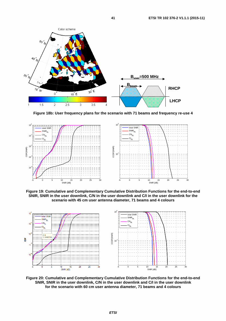
ETSI

ETSI TR 102 376-2 V1.1.1 (2015-11)41

Figure 18b: User frequency plans for the scenario with 71 beams and frequency re-use 4

Figure 19: Cumulative and Complementary Cumulative Distribution Functions for the end-to-end SNIR, SNIR in the user downlink, C/N in the user downlink and C/I in the user downlink for the

scenario with 45 cm user antenna diameter, 71 beams and 4 colours

Figure 20: Cumulative and Complementary Cumulative Distribution Functions for the end-to-end SNIR, SNIR in the user downlink, C/N in the user downlink and C/I in the user downlink

for the scenario with 60 cm user antenna diameter, 71 beams and 4 colours

Buser=500 MHz

RHCP

LHCP

Bbeam

-5 0 5 10 15 20 25 30

10-4

10-3

10-2

10-1

100

SNIR [dB]

CD

F(S

NIR

)

total SNIR

SNIRDL

CNDL

CIDL

-5 0 5 10 15 20 25 30

10-1

100

SNIR [dB]

CC

DF

(SN

IR)

total SNIR

SNIRDL

CNDL

CIDL

-5 0 5 10 15 20 25 30

10-1

100

SNIR [dB]

CC

DF

(SN

IR)

total SNIR

SNIRDL

CNDL

CIDL

ETSI

ETSI TR 102 376-2 V1.1.1 (2015-11)42

Figure 21: Cumulative and Complementary Cumulative Distribution Functions for the end-to-end SNIR, SNIR in the user downlink, C/N in the user downlink and C/I in the user downlink

for the scenario with 1 m user antenna diameter, 71 beams and 4 colours

From these results it can be seen that this system is C/N limited (the contribution of the intra-system interference to the total SNIR is marginal) and the range of SNIR over time and over the coverage for the typical availability figures is from about , 4 dB (at 99,7 % of the CDF) up to 11 dB (at 99 % of the CCDF) for the 45 cm user antenna, 6 dB (at 99,7 % of the CDF) up to 13 dB (at 99 % of the CCDF) for the 60 cm user antenna and 9 (at 99,7 % of the CDF) dB to 15 dB (at 99 % of the CCDF) for the 1 m user terminal antenna.

4.4.2.1.2.2 71 beams with a 2 colours scheme

This scenario has been selected to provide an example of network where co-channel interference mitigation techniques could be tested. It is a derivation of the short term network described above by pushing the number of colours to 2. This also allows to use one TWTA per beam in single carrier mode.

1) Gateway:

- Feeder link bandwidth in Ka-band: 2 GHz in two polarizations

- Gateway HPA saturated power: 1000 W; OBO = 6 dB

2) Satellite:

- TWTA saturated Power (single carrier):: 90 W

- One carrier per beam and per TWTA.

- IBO = 0,7 dB

- 71 beams with 4,3 dB triple-point

3) User Bandwidth: 500 MHz in two circular polarizations

4) Beam Bandwidth: 500 MHz

5) User Terminal:

- Antenna Diameter: 0,6 m

The color scheme over the coverage and user link frequency plans are depicted in the following figures while Figure 24 report the simulated SNIR CDF and CCDF distributions over the coverage and over time.

-5 0 5 10 15 20 25 30

10-1

100

SNIR [dB]

CC

DF

(SN

IR)

total SNIR

SNIRDL

CNDL

CIDL

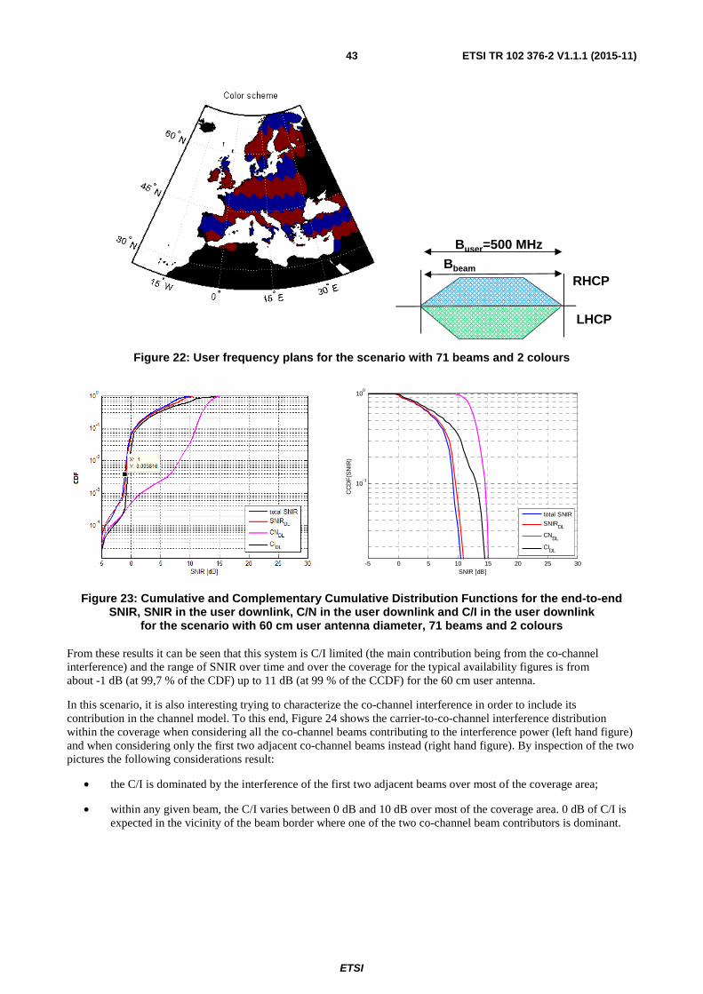
ETSI

ETSI TR 102 376-2 V1.1.1 (2015-11)43

Figure 22: User frequency plans for the scenario with 71 beams and 2 colours

Figure 23: Cumulative and Complementary Cumulative Distribution Functions for the end-to-end SNIR, SNIR in the user downlink, C/N in the user downlink and C/I in the user downlink

for the scenario with 60 cm user antenna diameter, 71 beams and 2 colours

From these results it can be seen that this system is C/I limited (the main contribution being from the co-channel interference) and the range of SNIR over time and over the coverage for the typical availability figures is from about -1 dB (at 99,7 % of the CDF) up to 11 dB (at 99 % of the CCDF) for the 60 cm user antenna.

In this scenario, it is also interesting trying to characterize the co-channel interference in order to include its contribution in the channel model. To this end, Figure 24 shows the carrier-to-co-channel interference distribution within the coverage when considering all the co-channel beams contributing to the interference power (left hand figure) and when considering only the first two adjacent co-channel beams instead (right hand figure). By inspection of the two pictures the following considerations result:

• the C/I is dominated by the interference of the first two adjacent beams over most of the coverage area;

• within any given beam, the C/I varies between 0 dB and 10 dB over most of the coverage area. 0 dB of C/I is expected in the vicinity of the beam border where one of the two co-channel beam contributors is dominant.

Buser=500 MHz

RHCP

LHCP

Bbeam

-5 0 5 10 15 20 25 30

10-1

100

SNIR [dB]

CC

DF

(SN

IR)

total SNIR

SNIRDL

CNDL

CIDL

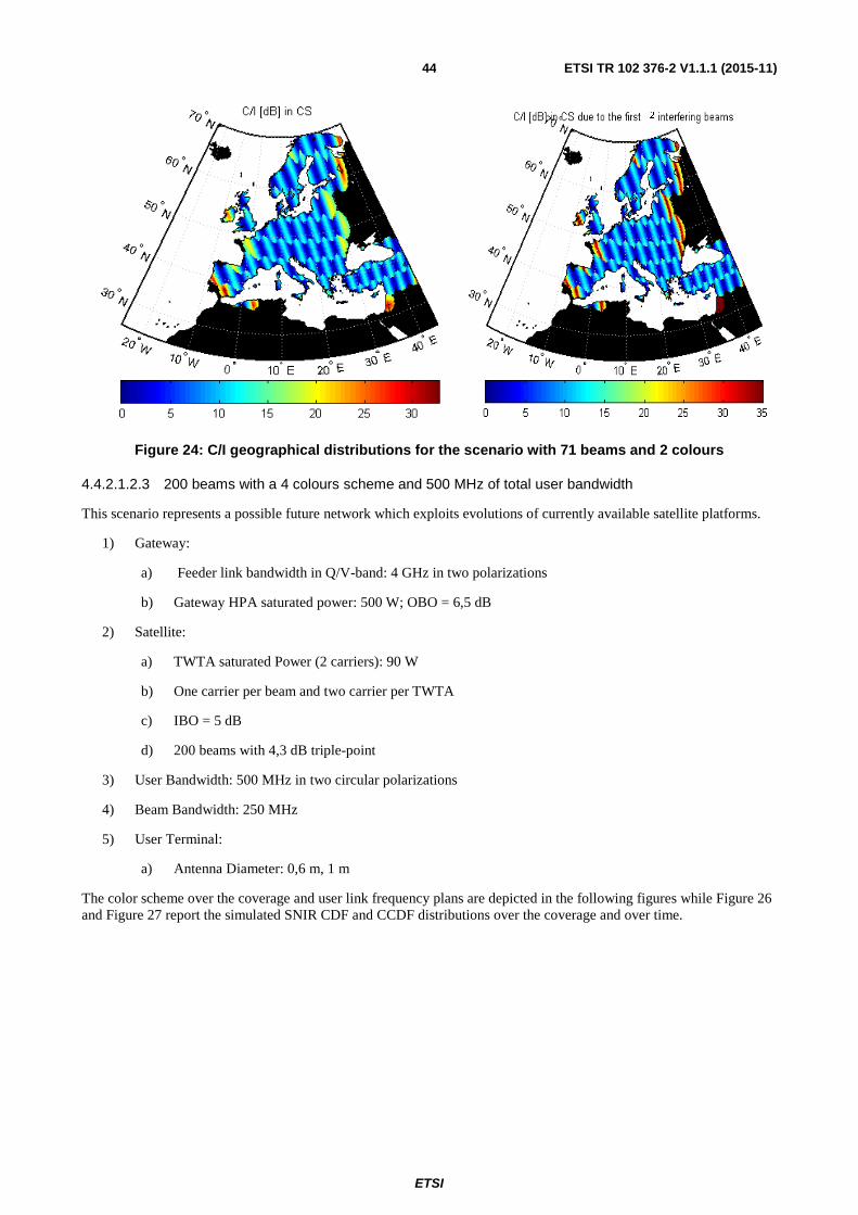
ETSI

ETSI TR 102 376-2 V1.1.1 (2015-11)44

Figure 24: C/I geographical distributions for the scenario with 71 beams and 2 colours

4.4.2.1.2.3 200 beams with a 4 colours scheme and 500 MHz of total user bandwidth

This scenario represents a possible future network which exploits evolutions of currently available satellite platforms.

1) Gateway:

a) Feeder link bandwidth in Q/V-band: 4 GHz in two polarizations

b) Gateway HPA saturated power: 500 W; OBO = 6,5 dB

2) Satellite:

a) TWTA saturated Power (2 carriers): 90 W

b) One carrier per beam and two carrier per TWTA

c) IBO = 5 dB

d) 200 beams with 4,3 dB triple-point

3) User Bandwidth: 500 MHz in two circular polarizations

4) Beam Bandwidth: 250 MHz

5) User Terminal:

a) Antenna Diameter: 0,6 m, 1 m

The color scheme over the coverage and user link frequency plans are depicted in the following figures while Figure 26 and Figure 27 report the simulated SNIR CDF and CCDF distributions over the coverage and over time.

2

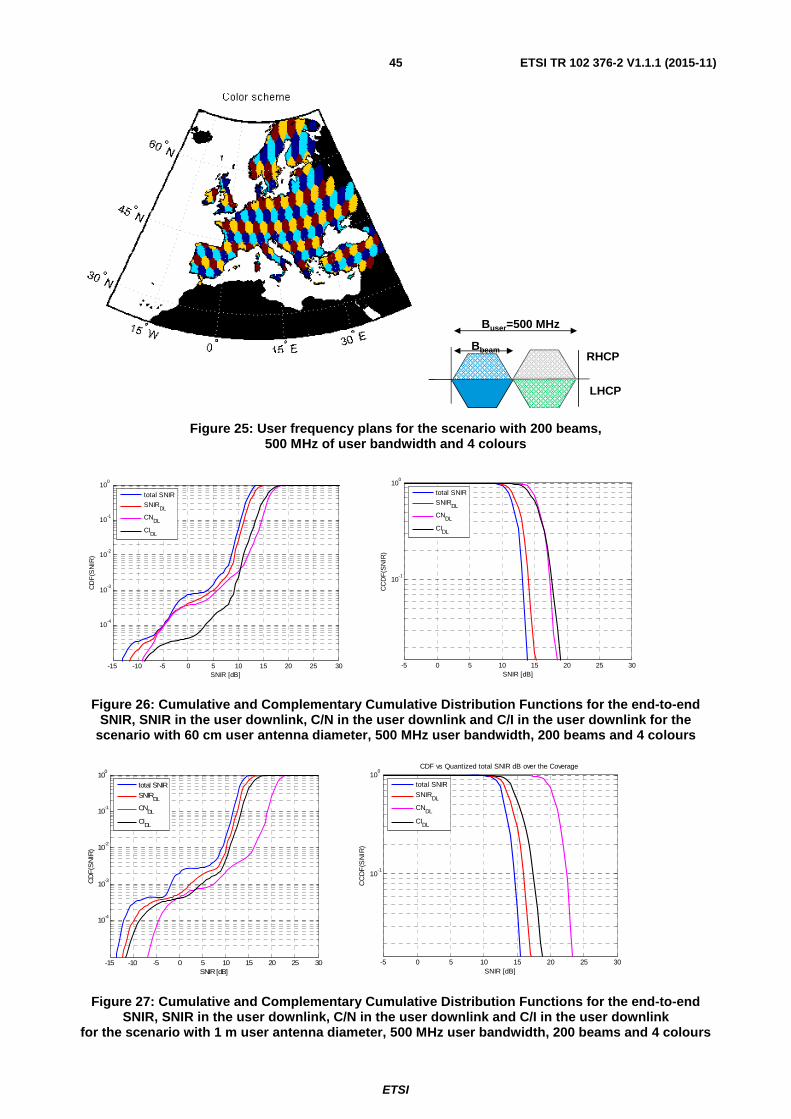
ETSI

ETSI TR 102 376-2 V1.1.1 (2015-11)45

Figure 25: User frequency plans for the scenario with 200 beams, 500 MHz of user bandwidth and 4 colours

Figure 26: Cumulative and Complementary Cumulative Distribution Functions for the end-to-end SNIR, SNIR in the user downlink, C/N in the user downlink and C/I in the user downlink for the

scenario with 60 cm user antenna diameter, 500 MHz user bandwidth, 200 beams and 4 colours

Figure 27: Cumulative and Complementary Cumulative Distribution Functions for the end-to-end SNIR, SNIR in the user downlink, C/N in the user downlink and C/I in the user downlink

for the scenario with 1 m user antenna diameter, 500 MHz user bandwidth, 200 beams and 4 colours

Buser=500 MHz

RHCP

LHCP

Bbeam

-15 -10 -5 0 5 10 15 20 25 30

10-4

10-3

10-2

10-1

100

SNIR [dB]

CD

F(S

NIR

)

total SNIR

SNIRDL

CNDL

CIDL

-5 0 5 10 15 20 25 30

10-1

100

SNIR [dB]

CC

DF

(SN

IR)

total SNIR

SNIRDL

CNDL

CIDL

-15 -10 -5 0 5 10 15 20 25 30

10-4

10-3

10-2

10-1

100

SNIR [dB]

CD

F(S

NIR

)

total SNIR

SNIRDL

CNDL

CIDL

-5 0 5 10 15 20 25 30

10-1

100

CDF vs Quantized total SNIR dB over the Coverage

SNIR [dB]

CC

DF

(SN

IR)

total SNIR

SNIRDL

CNDL

CIDL

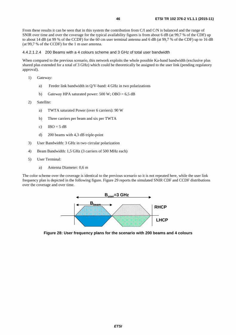
ETSI

ETSI TR 102 376-2 V1.1.1 (2015-11)46

From these results it can be seen that in this system the contribution from C/I and C/N is balanced and the range of SNIR over time and over the coverage for the typical availability figures is from about 6 dB (at 99,7 % of the CDF) up to about 14 dB (at 99 % of the CCDF) for the 60 cm user terminal antenna and 6 dB (at 99,7 % of the CDF) up to 16 dB (at 99,7 % of the CCDF) for the 1 m user antenna.

4.4.2.1.2.4 200 Beams with a 4 colours scheme and 3 GHz of total user bandwidth

When compared to the previous scenario, this network exploits the whole possible Ka-band bandwidth (exclusive plus shared plus extended for a total of 3 GHz) which could be theoretically be assigned to the user link (pending regulatory approval).

1) Gateway:

a) Feeder link bandwidth in Q/V-band: 4 GHz in two polarizations

b) Gateway HPA saturated power: 500 W; OBO = 6,5 dB

2) Satellite:

a) TWTA saturated Power (over 6 carriers): 90 W

b) Three carriers per beam and six per TWTA

c) IBO = 5 dB

d) 200 beams with 4,3 dB triple-point

3) User Bandwidth: 3 GHz in two circular polarization

4) Beam Bandwidth: 1,5 GHz (3 carriers of 500 MHz each)

5) User Terminal:

a) Antenna Diameter: 0,6 m

The color scheme over the coverage is identical to the previous scenario so it is not repeated here, while the user link frequency plan is depicted in the following figure. Figure 29 reports the simulated SNIR CDF and CCDF distributions over the coverage and over time.

Figure 28: User frequency plans for the scenario with 200 beams and 4 colours

Buser=3 GHz

RHCP

LHCP

Bbeam

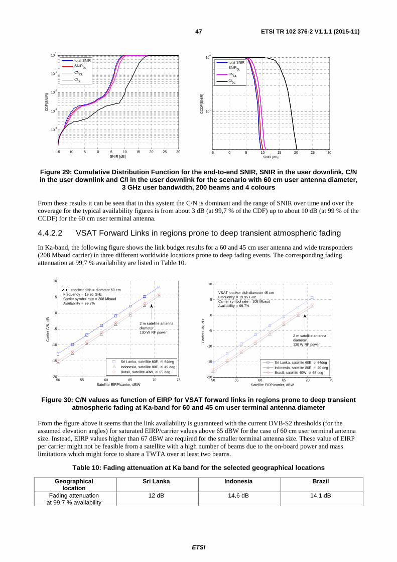
ETSI

ETSI TR 102 376-2 V1.1.1 (2015-11)47

Figure 29: Cumulative Distribution Function for the end-to-end SNIR, SNIR in the user downlink, C/N in the user downlink and C/I in the user downlink for the scenario with 60 cm user antenna diameter,

3 GHz user bandwidth, 200 beams and 4 colours

From these results it can be seen that in this system the C/N is dominant and the range of SNIR over time and over the coverage for the typical availability figures is from about 3 dB (at 99,7 % of the CDF) up to about 10 dB (at 99 % of the CCDF) for the 60 cm user terminal antenna.

4.4.2.2 VSAT Forward Links in regions prone to deep transient atmospheric fading

In Ka-band, the following figure shows the link budget results for a 60 and 45 cm user antenna and wide transponders (208 Mbaud carrier) in three different worldwide locations prone to deep fading events. The corresponding fading attenuation at 99,7 % availability are listed in Table 10.

Figure 30: C/N values as function of EIRP for VSAT forward links in regions prone to deep transient atmospheric fading at Ka-band for 60 and 45 cm user terminal antenna diameter

From the figure above it seems that the link availability is guaranteed with the current DVB-S2 thresholds (for the assumed elevation angles) for saturated EIRP/carrier values above 65 dBW for the case of 60 cm user terminal antenna size. Instead, EIRP values higher than 67 dBW are required for the smaller terminal antenna size. These value of EIRP per carrier might not be feasible from a satellite with a high number of beams due to the on-board power and mass limitations which might force to share a TWTA over at least two beams.

Table 10: Fading attenuation at Ka band for the selected geographical locations

Geographical location

Sri Lanka Indonesia Brazil

Fading attenuation at 99,7 % availability

12 dB 14,6 dB 14,1 dB

-15 -10 -5 0 5 10 15 20 25 30

10-4

10-3

10-2

10-1

100

SNIR [dB]

CD

F(S

NIR

)

total SNIR

SNIRDL

CNDL

CIDL

-5 0 5 10 15 20 25 30

10-1

100

SNIR [dB]

CC

DF

(SN

IR)

total SNIR

SNIRDL

CNDL

CIDL

50 55 60 65 70 75-20

-15

-10

-5

0

5

10

Satellite EIRP/carrier, dBW

Car

rier

C/N

, dB

Sri Lanka, satellite 60E, el 64deg

Indonesia, satellite 80E, el 49 degBrasil, satellite 40W, el 65 deg

DTH receiver dish = diameter 60 cmFrequency = 19.95 GHzCarrier symbol rate = 208 MbaudAvailability = 99.7%

2 m satellite antennadiameter130 W RF power

VSAT

50 55 60 65 70 75-20

-15

-10

-5

0

5

10

Satellite EIRP/carrier, dBW

Car

rier

C/N

, dB

Sri Lanka, satellite 60E, el 64deg

Indonesia, satellite 80E, el 49 degBrasil, satellite 40W, el 65 deg

VSAT receiver dish diameter 45 cmFrequency = 19.95 GHzCarrier symbol rate = 208 MbaudAvailability = 99.7%

2 m satellite antennadiameter130 W RF power

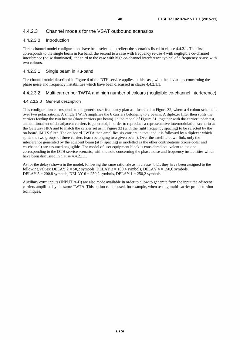
ETSI

ETSI TR 102 376-2 V1.1.1 (2015-11)48

4.4.2.3 Channel models for the VSAT outbound scenarios

4.4.2.3.0 Introduction

Three channel model configurations have been selected to reflect the scenarios listed in clause 4.4.2.1. The first corresponds to the single beam in Ku band, the second to a case with frequency re-use 4 with negligible co-channel interference (noise dominated), the third to the case with high co-channel interference typical of a frequency re-use with two colours.

4.4.2.3.1 Single beam in Ku-band

The channel model described in Figure 4 of the DTH service applies in this case, with the deviations concerning the phase noise and frequency instabilities which have been discussed in clause 4.4.2.1.1.

4.4.2.3.2 Multi-carrier per TWTA and high number of colours (negligible co-channel interference)

4.4.2.3.2.0 General description

This configuration corresponds to the generic user frequency plan as illustrated in Figure 32, where a 4 colour scheme is over two polarizations. A single TWTA amplifies the 6 carriers belonging to 2 beams. A diplexer filter then splits the carriers feeding the two beams (three carriers per beam). In the model of Figure 31, together with the carrier under test, an additional set of six adjacent carriers is generated, in order to reproduce a representative intermodulation scenario at the Gateway HPA and to match the carrier set as in Figure 32 (with the right frequency spacing) to be selected by the on-board IMUX filter. The on-board TWTA then amplifies six carriers in total and it is followed by a diplexer which splits the two groups of three carriers (each belonging to a given beam). Over the satellite down-link, only the interference generated by the adjacent beam (at fB spacing) is modelled as the other contributions (cross-polar and co-channel) are assumed negligible. The model of user equipment block is considered equivalent to the one corresponding to the DTH service scenario, with the note concerning the phase noise and frequency instabilities which have been discussed in clause 4.4.2.1.1.

As for the delays shown in the model, following the same rationale as in clause 4.4.1, they have been assigned to the following values: DELAY 2 = 50,2 symbols, DELAY 3 = 100,4 symbols, DELAY 4 = 150,6 symbols, DELAY 5 = 200,8 symbols, DELAY 6 = 250,2 symbols, DELAY 1 = 250,2 symbols.

Auxiliary extra inputs (INPUT A-D) are also made available in order to allow to generate from the input the adjacent carriers amplified by the same TWTA. This option can be used, for example, when testing multi-carrier pre-distortion techniques.

ETSI

ETSI TR 102 376-2 V1.1.1 (2015-11)49

Figure 31: Channel model for VSAT outbound with multi-carrier per TWTA configuration and frequency re-use 4

Figure 32: User frequency and carrier plans for the VSAT outbound scenario with multi-carrier per TWTA configuration and frequency re-use 4

4.4.2.3.2.1 GW HPA

As shown in Figure 5 on the DTH service.

INPUT

OUTPUT

INPUT A

INPUT B

INPUT C

INPUT D

INPUT E

DELAY 1 X

ej2 fbt

ADJACENT

BEAM

INTERF

SATELLITE TXP

IMUX TWTA DIPLEXER

RECEIVER

AMPLITUDE

DISTORTIONS

AWGN

X

PHASE AND FREQ.

ERRORS

GW

HPA

DELAY 3

X

X

X

X

e-j2 fct

e-j4 fct

ej2 fb-fc)t

ej2 fbt

GROUND STATION

USER

EQUIPMENT

RECEIVER

X

ej2 fb+fc)t

DELAY 2

DELAY 4

DELAY 5

DELAY 6

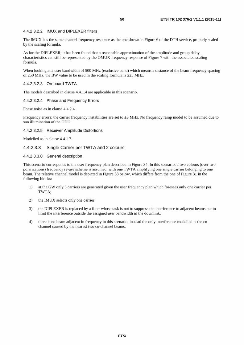
ETSI

ETSI TR 102 376-2 V1.1.1 (2015-11)50

4.4.2.3.2.2 IMUX and DIPLEXER filters

The IMUX has the same channel frequency response as the one shown in Figure 6 of the DTH service, properly scaled by the scaling formula.

As for the DIPLEXER, it has been found that a reasonable approximation of the amplitude and group delay characteristics can still be represented by the OMUX frequency response of Figure 7 with the associated scaling formula.

When looking at a user bandwidth of 500 MHz (exclusive band) which means a distance of the beam frequency spacing of 250 MHz, the BW value to be used in the scaling formula is 225 MHz.

4.4.2.3.2.3 On-board TWTA

The models described in clause 4.4.1.4 are applicable in this scenario.

4.4.2.3.2.4 Phase and Frequency Errors

Phase noise as in clause 4.4.2.4

Frequency errors: the carrier frequency instabilities are set to ±3 MHz. No frequency ramp model to be assumed due to sun illumination of the ODU.

4.4.2.3.2.5 Receiver Amplitude Distortions

Modelled as in clause 4.4.1.7.

4.4.2.3.3 Single Carrier per TWTA and 2 colours

4.4.2.3.3.0 General description

This scenario corresponds to the user frequency plan described in Figure 34. In this scenario, a two colours (over two polarizations) frequency re-use scheme is assumed, with one TWTA amplifying one single carrier belonging to one beam. The relative channel model is depicted in Figure 33 below, which differs from the one of Figure 31 in the following blocks:

1) at the GW only 5 carriers are generated given the user frequency plan which foresees only one carrier per TWTA;

2) the IMUX selects only one carrier;

3) the DIPLEXER is replaced by a filter whose task is not to suppress the interference to adjacent beams but to limit the interference outside the assigned user bandwidth in the downlink;

4) there is no beam adjacent in frequency in this scenario, instead the only interference modelled is the co-channel caused by the nearest two co-channel beams.

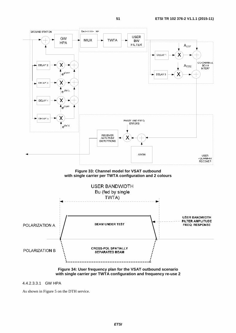
ETSI

ETSI TR 102 376-2 V1.1.1 (2015-11)51

Figure 33: Channel model for VSAT outbound with single carrier per TWTA configuration and 2 colours

Figure 34: User frequency plan for the VSAT outbound scenario with single carrier per TWTA configuration and frequency re-use 2

4.4.2.3.3.1 GW HPA

As shown in Figure 5 on the DTH service.

ETSI

ETSI TR 102 376-2 V1.1.1 (2015-11)52

4.4.2.3.3.2 IMUX and User Bandwidth Filter

The IMUX has the same channel frequency response as the one shown in Figure 6 of the DTH service, properly scaled by the scaling formula.

As for the User Bandwidth filter as a first approximation, the amplitude and group delay characteristics of the OMUX frequency response of Figure 7 with the associated scaling formula, can be used. When looking at a user bandwidth of 500 MHz (exclusive band) the BW to be used is 450 MHz in order to provide the right suppression outside the allocated bandwidth.

4.4.2.3.3.3 TWTA

The models described in clause 4.4.1.4 are applicable also in this scenario.

4.4.2.3.3.4 Co-channel Interference Model

Following the scenario described in clause 4.4.2.1.2.2, the following two cases are recommended for testing.

Table 11: Recommended C/I values for the co-channel beam contributors

case C/I from co-channel beam 1 C/I from co-channel beam 2 1 0 dB 10 dB 2 4 dB 6 dB

4.4.2.3.3.5 Phase and Frequency Error

Phase noise as in clause 4.4.2.4.

Frequency errors: the carrier frequency instabilities to be set to ±3 MHz. No frequency ramp model assumed due to sun illumination of the ODU.

4.4.2.3.3.6 Receiver Amplitude Distortions

Modelled as in clause 4.4.1.7.

4.4.2.4 Phase Noise Masks

A number of non-DTH phase noise masks are proposed according to the band (Ku and Ka) and the state of the art (2012) and older equipments (2000). The contributions from the GW (uplink), the satellite payload as well as the receiver (downlink) have been taken into account.

Table 12: Phase noise masks proposed for non- DTH services

Offset (Hz)

PROFILE "2000-Ku- Non DTH" SSB (dBc/Hz)

uplink satellite downlink tot-equiv 10 -30 -33 -30 -28,24

100 -60 -62 -60 -58,10 1 K -70 -81 -70 -68,49 10 K -80 -84 -80 -78,33

100 K -90 -94 -90 -88,33 1 M -90 -94 -90 -88,33

10 M -90 -94 -90 -88,33

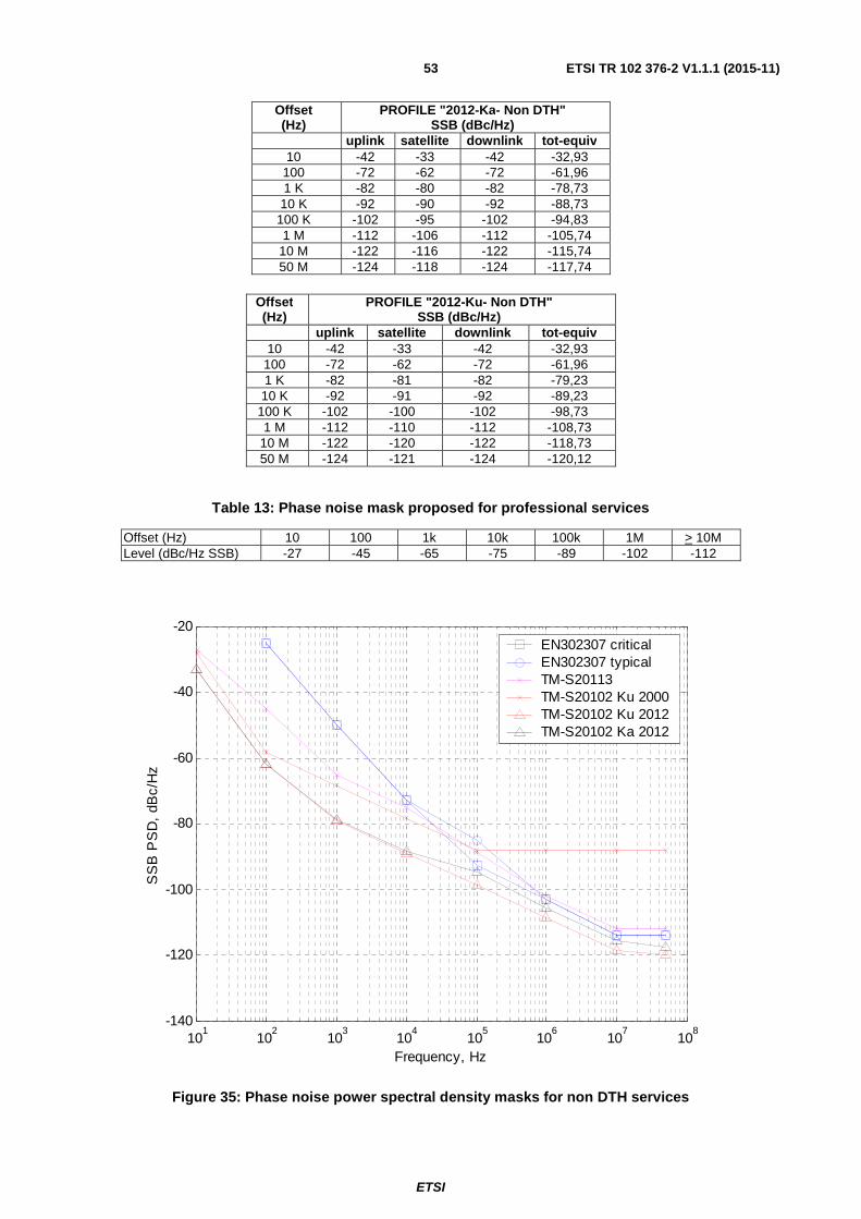
ETSI

ETSI TR 102 376-2 V1.1.1 (2015-11)53

Offset (Hz)

PROFILE "2012-Ka- Non DTH" SSB (dBc/Hz)

uplink satellite downlink tot-equiv 10 -42 -33 -42 -32,93

100 -72 -62 -72 -61,96 1 K -82 -80 -82 -78,73 10 K -92 -90 -92 -88,73

100 K -102 -95 -102 -94,83 1 M -112 -106 -112 -105,74

10 M -122 -116 -122 -115,74 50 M -124 -118 -124 -117,74

Table 13: Phase noise mask proposed for professional services

Offset (Hz) 10 100 1k 10k 100k 1M > 10M Level (dBc/Hz SSB) -27 -45 -65 -75 -89 -102 -112

Figure 35: Phase noise power spectral density masks for non DTH services

101

102

103

104

105

106

107

108

-140

-120

-100

-80

-60

-40

-20

Frequency, Hz

SS

B P

SD

, dB

c/H

z

EN302307 criticalEN302307 typicalTM-S20113TM-S20102 Ku 2000TM-S20102 Ku 2012TM-S20102 Ka 2012

Offset (Hz)

PROFILE "2012-Ku- Non DTH" SSB (dBc/Hz)

uplink satellite downlink tot-equiv 10 -42 -33 -42 -32,93

100 -72 -62 -72 -61,96 1 K -82 -81 -82 -79,23 10 K -92 -91 -92 -89,23

100 K -102 -100 -102 -98,73 1 M -112 -110 -112 -108,73

10 M -122 -120 -122 -118,73 50 M -124 -121 -124 -120,12

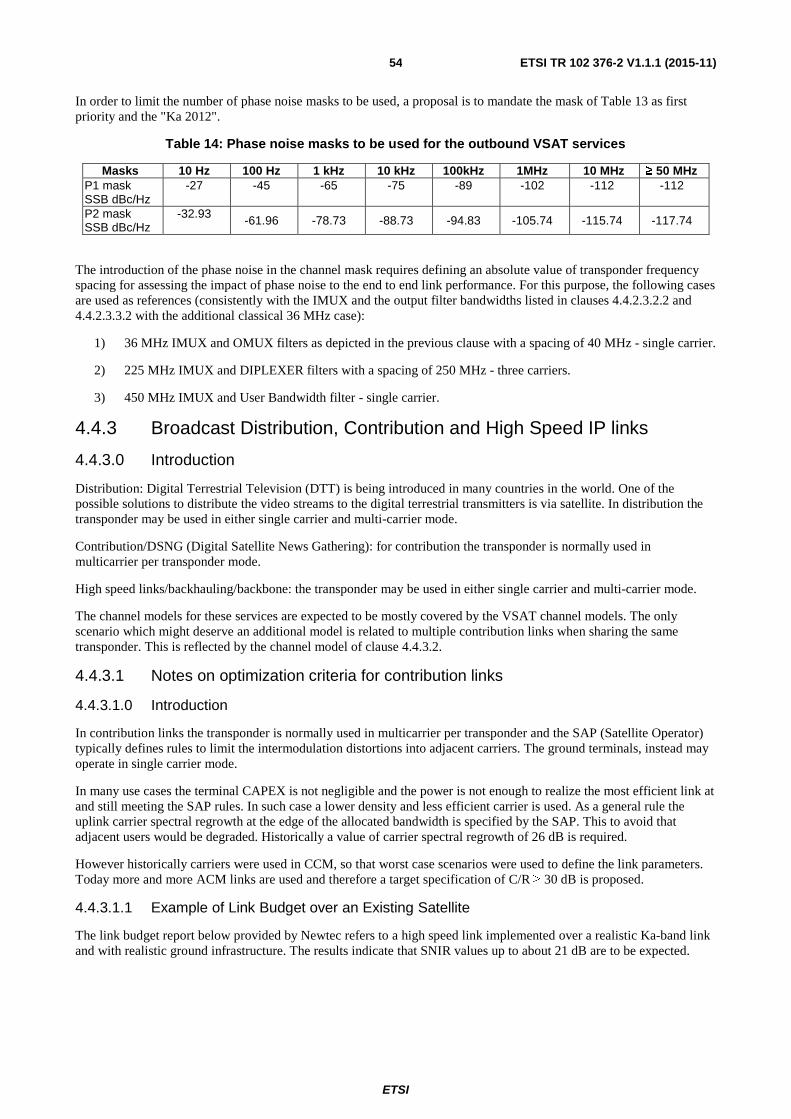
ETSI

ETSI TR 102 376-2 V1.1.1 (2015-11)54

In order to limit the number of phase noise masks to be used, a proposal is to mandate the mask of Table 13 as first priority and the "Ka 2012".

Table 14: Phase noise masks to be used for the outbound VSAT services

Masks 10 Hz 100 Hz 1 kHz 10 kHz 100kHz 1MHz 10 MHz ≥ 50 MHz P1 mask SSB dBc/Hz

-27 -45 -65 -75 -89 -102 -112 -112

P2 mask SSB dBc/Hz

-32.93 -61.96 -78.73 -88.73 -94.83 -105.74 -115.74 -117.74

The introduction of the phase noise in the channel mask requires defining an absolute value of transponder frequency spacing for assessing the impact of phase noise to the end to end link performance. For this purpose, the following cases are used as references (consistently with the IMUX and the output filter bandwidths listed in clauses 4.4.2.3.2.2 and 4.4.2.3.3.2 with the additional classical 36 MHz case):

1) 36 MHz IMUX and OMUX filters as depicted in the previous clause with a spacing of 40 MHz - single carrier.

2) 225 MHz IMUX and DIPLEXER filters with a spacing of 250 MHz - three carriers.

3) 450 MHz IMUX and User Bandwidth filter - single carrier.

4.4.3 Broadcast Distribution, Contribution and High Speed IP links

4.4.3.0 Introduction

Distribution: Digital Terrestrial Television (DTT) is being introduced in many countries in the world. One of the possible solutions to distribute the video streams to the digital terrestrial transmitters is via satellite. In distribution the transponder may be used in either single carrier and multi-carrier mode.

Contribution/DSNG (Digital Satellite News Gathering): for contribution the transponder is normally used in multicarrier per transponder mode.

High speed links/backhauling/backbone: the transponder may be used in either single carrier and multi-carrier mode.

The channel models for these services are expected to be mostly covered by the VSAT channel models. The only scenario which might deserve an additional model is related to multiple contribution links when sharing the same transponder. This is reflected by the channel model of clause 4.4.3.2.

4.4.3.1 Notes on optimization criteria for contribution links

4.4.3.1.0 Introduction

In contribution links the transponder is normally used in multicarrier per transponder and the SAP (Satellite Operator) typically defines rules to limit the intermodulation distortions into adjacent carriers. The ground terminals, instead may operate in single carrier mode.

In many use cases the terminal CAPEX is not negligible and the power is not enough to realize the most efficient link at and still meeting the SAP rules. In such case a lower density and less efficient carrier is used. As a general rule the uplink carrier spectral regrowth at the edge of the allocated bandwidth is specified by the SAP. This to avoid that adjacent users would be degraded. Historically a value of carrier spectral regrowth of 26 dB is required.

However historically carriers were used in CCM, so that worst case scenarios were used to define the link parameters. Today more and more ACM links are used and therefore a target specification of C/R ≥ 30 dB is proposed.

4.4.3.1.1 Example of Link Budget over an Existing Satellite

The link budget report below provided by Newtec refers to a high speed link implemented over a realistic Ka-band link and with realistic ground infrastructure. The results indicate that SNIR values up to about 21 dB are to be expected.

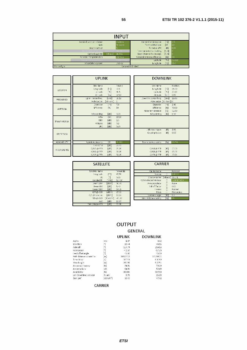
ETSI

ETSI TR 102 376-2 V1.1.1 (2015-11)55

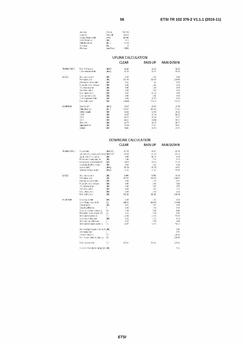
ETSI

ETSI TR 102 376-2 V1.1.1 (2015-11)56

ETSI

ETSI TR 102 376-2 V1.1.1 (2015-11)57

4.4.3.2 A Channel Model for Contribution Links

4.4.3.2.0 General description

This scenario corresponds to a very large number of possible models. However, many of these models could be fairly represented by the ones that address the previous scenarios (i.e. a technique devised to optimize those scenario would also maximize the performance within the many contribution, distribution and IP high speed links). In the following, an additional model is added as deemed to possibly address additional optimization techniques.

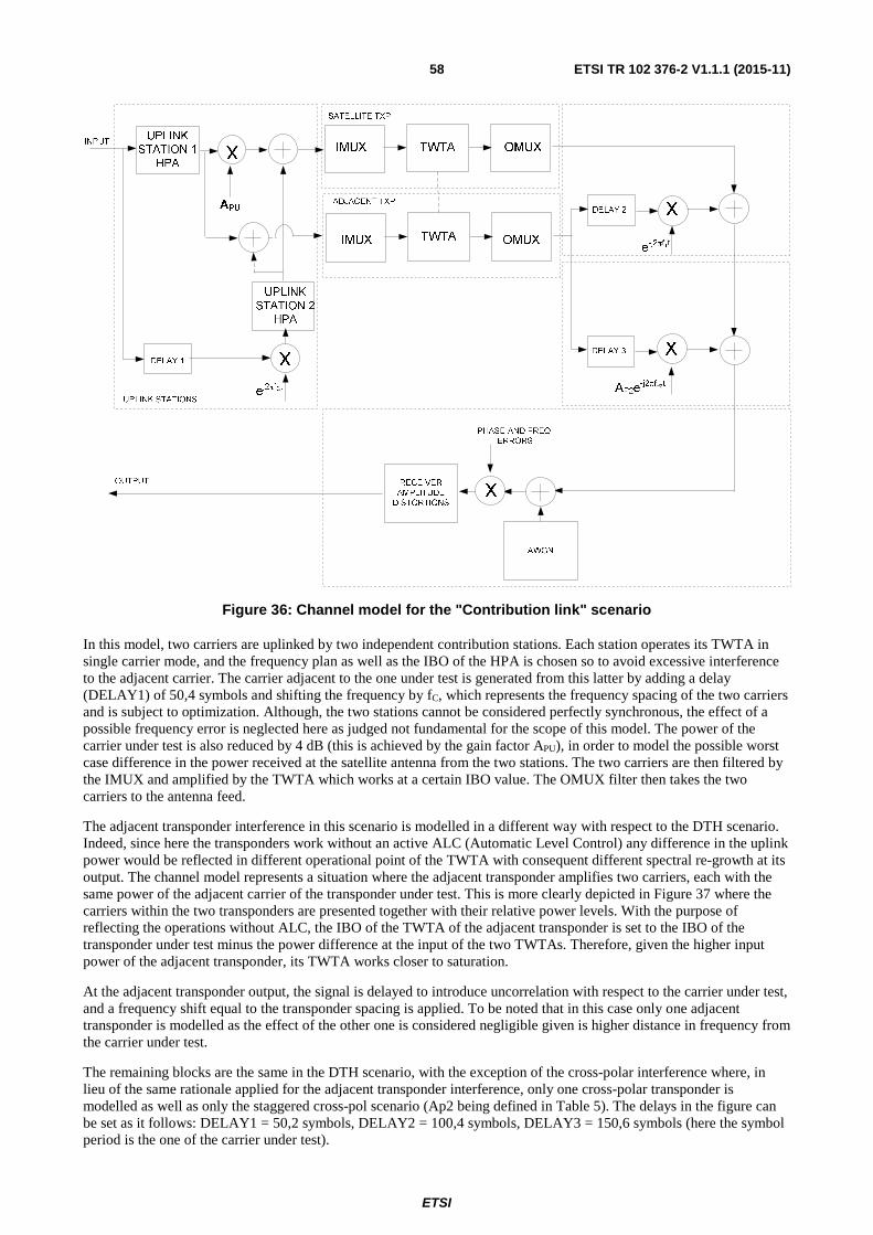
ETSI

ETSI TR 102 376-2 V1.1.1 (2015-11)58

Figure 36: Channel model for the "Contribution link" scenario

In this model, two carriers are uplinked by two independent contribution stations. Each station operates its TWTA in single carrier mode, and the frequency plan as well as the IBO of the HPA is chosen so to avoid excessive interference to the adjacent carrier. The carrier adjacent to the one under test is generated from this latter by adding a delay (DELAY1) of 50,4 symbols and shifting the frequency by fC, which represents the frequency spacing of the two carriers and is subject to optimization. Although, the two stations cannot be considered perfectly synchronous, the effect of a possible frequency error is neglected here as judged not fundamental for the scope of this model. The power of the carrier under test is also reduced by 4 dB (this is achieved by the gain factor APU), in order to model the possible worst case difference in the power received at the satellite antenna from the two stations. The two carriers are then filtered by the IMUX and amplified by the TWTA which works at a certain IBO value. The OMUX filter then takes the two carriers to the antenna feed.

The adjacent transponder interference in this scenario is modelled in a different way with respect to the DTH scenario. Indeed, since here the transponders work without an active ALC (Automatic Level Control) any difference in the uplink power would be reflected in different operational point of the TWTA with consequent different spectral re-growth at its output. The channel model represents a situation where the adjacent transponder amplifies two carriers, each with the same power of the adjacent carrier of the transponder under test. This is more clearly depicted in Figure 37 where the carriers within the two transponders are presented together with their relative power levels. With the purpose of reflecting the operations without ALC, the IBO of the TWTA of the adjacent transponder is set to the IBO of the transponder under test minus the power difference at the input of the two TWTAs. Therefore, given the higher input power of the adjacent transponder, its TWTA works closer to saturation.

At the adjacent transponder output, the signal is delayed to introduce uncorrelation with respect to the carrier under test, and a frequency shift equal to the transponder spacing is applied. To be noted that in this case only one adjacent transponder is modelled as the effect of the other one is considered negligible given is higher distance in frequency from the carrier under test.

The remaining blocks are the same in the DTH scenario, with the exception of the cross-polar interference where, in lieu of the same rationale applied for the adjacent transponder interference, only one cross-polar transponder is modelled as well as only the staggered cross-pol scenario (Ap2 being defined in Table 5). The delays in the figure can be set as it follows: DELAY1 = 50,2 symbols, DELAY2 = 100,4 symbols, DELAY3 = 150,6 symbols (here the symbol period is the one of the carrier under test).

ETSI

ETSI TR 102 376-2 V1.1.1 (2015-11)59

Figure 37: Transponder and carrier configuration for the channel model of the contribution link

4.4.3.2.1 GW HPA

As shown in Figure 5 on the DTH service.

4.4.3.2.2 IMUX and OMUX Filter

The IMUX and OMUX have the same channel frequency response as the one shown in Figure 6 and Figure 7 of the DTH service.

For this scenario, the main reference case to be simulated is the 36 MHz transponder where two independent uplink carrier fill up the entire transponder. However, just for the purpose of showing resilience w.r.t the phase noise, a case with underutilization of the transponder with two carriers of 1 MHz of bandwidth each, can also be simulated.

4.4.3.2.3 On-board TWTA

The models described in clause 4.4.1.4 are applicable in this scenario.

4.4.3.2.4 Phase and Frequency Errors

Phase noise model is derived from clause 4.4.2.4. However, for this scenario what was the P2 selection in that clause is considered instead more relevant here. Therefore, for professional links the priorities are reverted.

Table 15: Phase noise masks to be used for the Broadcast Distribution, Contribution and High Speed IP links

Masks 10 Hz 100 Hz 1 kHz 10 kHz 100 kHz 1 MHz 10 MHz ≥ 50 MHz P1 mask SSB dBc/Hz

-32,93 -61,96 -78,73 -88,73 -94,83 -105,74 -115,74 -117,74

P2 mask SSB dBc/Hz

-27 -45 -65 -75 -89 -102 -112 -112

Frequency errors: the carrier frequency instabilities to be set to ±1 MHz. No frequency ramp model assumed due to sun illumination of the ODU.

4.4.3.2.5 Receiver Amplitude Distortions

Modelled as in clause 4.4.1.7.

Ca

rrier u

nd

er te

st

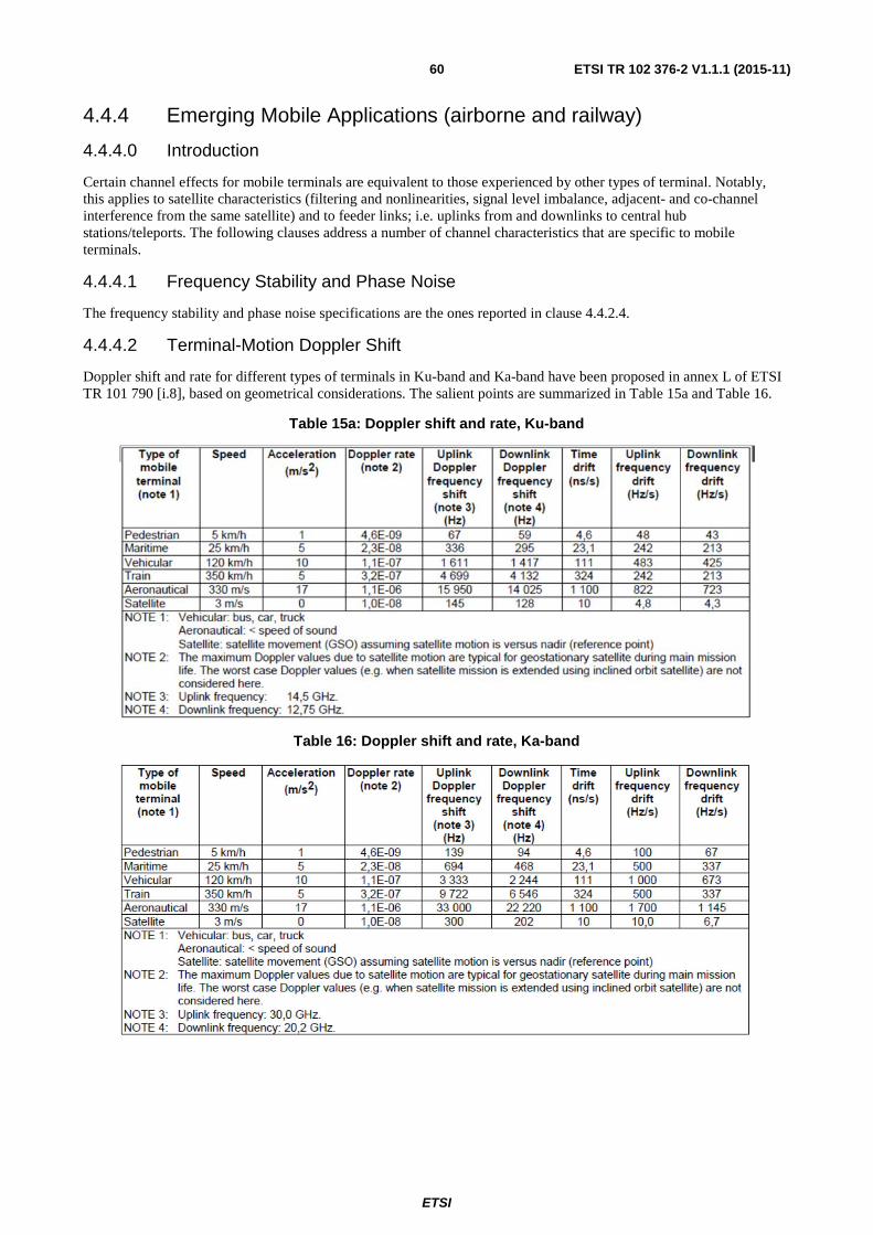
ETSI

ETSI TR 102 376-2 V1.1.1 (2015-11)60

4.4.4 Emerging Mobile Applications (airborne and railway)

4.4.4.0 Introduction

Certain channel effects for mobile terminals are equivalent to those experienced by other types of terminal. Notably, this applies to satellite characteristics (filtering and nonlinearities, signal level imbalance, adjacent- and co-channel interference from the same satellite) and to feeder links; i.e. uplinks from and downlinks to central hub stations/teleports. The following clauses address a number of channel characteristics that are specific to mobile terminals.

4.4.4.1 Frequency Stability and Phase Noise

The frequency stability and phase noise specifications are the ones reported in clause 4.4.2.4.

4.4.4.2 Terminal-Motion Doppler Shift

Doppler shift and rate for different types of terminals in Ku-band and Ka-band have been proposed in annex L of ETSI TR 101 790 [i.8], based on geometrical considerations. The salient points are summarized in Table 15a and Table 16.

Table 15a: Doppler shift and rate, Ku-band

Table 16: Doppler shift and rate, Ka-band

ETSI

ETSI TR 102 376-2 V1.1.1 (2015-11)61

The maximum offset and drift rates are both important for acquisition. For tracking, the drift rate is the most important, as any constant Doppler has presumably been compensated. In reality, the maximum drift rates cannot be sustained for long periods of time; otherwise the signal would drift completely out of the band. It is therefore proposed to model the carrier frequency offset as a sinusoidal variation with an amplitude corresponding to the maximum given in the applicable table above, and a period that results in a maximum rate of change as per the table. This can be envisaged as the situation that would exist if the terminal were to move in a circular pattern with the satellite at low elevation angle.

The frequency offset is given by:

⎟⎠

⎞⎜⎝

⎛Δ=ΔP

ttf f

π2cos)( max,

(1)

where Δf,max is the value from the table above (e.g. 22 220 Hz for an aeronautical terminal at 20,2 GHz) and P is the period of the variation. P can be determined by differentiating (1):

⎟⎠

⎞⎜⎝

⎛Δ−=Δ

∂∂

P

t

Ptf

tf ππ 2

sin2

)( max,

(2)

This will be maximized for values of t where the sin(.) term equals -1, i.e.:

maxmax,2

)(max DP

tft

f =Δ

=⎟⎠

⎞⎜⎝

⎛ Δ∂∂ π

(3)

where Dmax is the maximum drift from the table (e.g. 1 145 Hz/s for an aeronautical terminal at 20,2 GHz). Simple re-arrangement gives:

max

max,2

DP fΔ

=π

(4)

For the example, P = 2π × 22 200 / 1 145 = 121,82 s.

The timing drift rates are equivalent to symbol rate offsets and are best modelled as such.

4.4.4.3 Multipath Fading

For aeronautical applications in Ku- and Ka-band, where the antennas have significant directivity, multipath effects are of relatively minor importance when the plane is airborne - they are essentially limited to reflections from the airframe itself. Given the pointing geometry, reflections e.g. from the sea surface or other ground features are very minor. One measurement campaign [i.9] found that with aircraft manoeuvres in the normal range, this could be modelled as Rician fading with a K-factor of about 34 dB - in other words, negligible from the point of view of influence on the signal quality. It should be noted that the above results were obtained with an antenna aperture of about 25 cm; i.e. smaller than what would normally be used on commercial aircraft even today.

For train applications, multipath reflections can originate from terrain elements around the terminal, and cannot be ignored. Clause 11 of the DVB-RCS + M guidelines ETSI TR 102 768 [i.7] has a proposed model. According to that study, the fading is again Rician; with a typical K-factor of about 17 dB.

The same clause also provides expressions for the shape of the Doppler spectrum, conditioned on the antenna beam width. The shape of the Doppler spectrum however also depends on the angle between the direction of travel and the LOS to the satellite. With these conditions, the relative spectral densities provided in ETSI TR 102 768 [i.7] can be integrated and scaled to represent the desired K-factor.

4.4.4.4 Shadowing

For aeronautical applications, it was found in ETSI TR 102 768 [i.7] that normal manoeuvres would only create short-term shadowing (primarily by the wings) of perhaps 2-3 dB. Extreme manoeuvres were required to create significant fades of more than 10 dB; these can be considered outside the typical range for which the system would normally be designed.

ETSI

ETSI TR 102 376-2 V1.1.1 (2015-11)62

Shadowing and blockage are potentially severe problems for train applications, as in most other land mobile situations. Signal blockage by buildings, overpasses, tunnels etc. typically cannot be overcome by physical layer techniques alone. They will require some form of diversity - either spatial (e.g. satellite or antenna) or temporal (e.g. signal repetition or interleaving with higher-layer coding). A scheme using link-layer coding was adopted in DVB-RCS + M; this is described in clause 5.3 of ETSI TR 102 768 [i.7].

Unless a proposed scheme is believed to be particularly robust against shadowing and blockage (like long physical layer interleaving), the remedial actions will largely be independent of the underlying physical layer techniques. For the purpose of comparing candidate physical-layer schemes, it is therefore not initially considered necessary that the blocking channel or the corresponding countermeasures be modelled in detail.

If modelling of this is nonetheless preferred by a system proponent, indications of applicable blocking characteristics are given in clause 4.2.1 of ETSI TR 102 768 [i.7], based on the same study that produced the multipath models. In that case, the use of the parameters given there is recommended.

The physical layer should however support rapid re-acquisition following a short-duration blockage. In ETSI TR 102 768 [i.7], this is defined as a blockage with a duration of less than 1 second.

4.4.4.5 Adjacent Satellite Interference

Adjacent satellite interference depends mainly on the antenna pattern and on the achievable pointing accuracy. While not inherently specific to mobile terminals, the impact is often more pronounced than for other types of terminal, due to physical restrictions on the feasible aperture sizes.

For aeronautical applications representing for example commercial aircraft, it is suggested to compute adjacent-satellite interference based on the following three antenna apertures:

• A 30-cm circular-symmetric aperture, representing for example what is feasible on business jets.

• A 60-cm circular-symmetric aperture, representing for example a wide-body airliner. This can also be seen as an "average" of the situations that will exist for a non-symmetric aperture.

• An elliptical aperture with a minor axis (narrowest beamwidth) equivalent to a 120-cm circular aperture, and a major axis (largest beamwidth) corresponding to a 30-cm circular aperture. These antennas will typically be fixed-mounted on the aircraft fuselage; hence the orientation with respect to the geostationary arc will depend on the link geometry ("skew angle").

For train applications, a 60 cm circular-symmetric aperture can be used as reference.

For all antennas, a worst-case pointing error of 0,2° can be assumed.

When FSS frequencies are used, the orbit spacing should be assumed to be either 2° or 3°, according to frequency band and geographical region. When BSS frequencies are used, the assumptions in clause 4.4.1.5.1 should be applied.

The following expression is recommended for computing the gain of a symmetrical-aperture antenna. Let:

D = antenna diameter (m)

e = aperture efficiency (0...1), typically 0,6

λ = wavelength (m)

Θ = off-axis angle (radians)

J1(x) = first order Bessel function of the first kind

Let:

)sin(θλ

πμ D=

(5)

ETSI

ETSI TR 102 376-2 V1.1.1 (2015-11)63

The antenna gain (linear) is then:

2

1

2)(

2 ⎥⎦

⎤⎢⎣

⎡ ×⎟⎠

⎞⎜⎝

⎛×=μμ

λπ JD

eG

(6)

4.4.4.6 SNR Dynamics

4.4.4.6.0 General description

This clause provides considerations of the SNR characteristics of the channel experienced by satellite terminals mounted on high-speed mobile platforms. The contribution addresses primarily aircraft and high-speed trains.

This topic has been addressed previously. In the context of DVB-RCS + M, assessments focussed on the need for spread-spectrum operation were carried out, based in part on an ESA-sponsored study. The findings are reported for example in [i.11]. It should be noted however that this study was assuming current-generation space segment; while the principles are still completely valid, this assumption does influence the detailed results to some degree. Also, the return link considerations in [i.11] address TDMA transmissions. For the purpose of this analysis, it is interesting to apply continuous-carrier techniques not only to the forward link, but also to return links from mobile terminals to a central hub.

In the forward link, spread-spectrum is employed as an interference mitigation technique. In the return link, it is employed primarily as a way of assuring compliance with regulatory emission requirements, in particular off-axis EIRP density. In both cases, the net result is the need for operation at low signal-to-noise ratio (Ec/N0).

One significant development that has occurred since the preparation of [i.11] is the publication of a regulatory framework for terminals mounted on mobile platforms operating in Ka-band, ETSI EN 303 978 [i.12]. For the purpose of the present assessment, the provisions of highest interest in the present document are the off-axis EIRP density regulations. These follow the same roll-off as other masks intended to operate with 2° orbit spacing.

The following clause summarizes the results from [i.11] and extends them to next-generation space segment.

In assessing the results in the following sub-clauses, it should be recalled that the smallest apertures considered (~ 30 cm) not only represent actual antennas, such as may be found for example on business jets. They also represent typical values of the smallest dimension of non-uniform apertures such as flat-panel antennas. Since such antennas are most often mounted in a fixed relation to the platform (airframe, train carriage), the orientation with respect to the geostationary arc depends on the link geometry ("skew angle"). Hence the ability to operate with (the equivalent of) the very small apertures is important for many applications, even when some physical dimensions of the antenna are substantially bigger.

4.4.4.6.1 Forward Link

For the forward link, [i.11] concludes that systems operating in regional or smaller beams only require spreading for extremely small user terminal apertures (< 30 cm). Systems operating in large ("global") beams however can need spreading for apertures smaller than about 50 cm. In this context, the need for spreading is based on the feasibility of closing a standard DVB-S2 link operating at QPSK r = 1/4. The highest identified spreading factor required for a 30 cm antenna is 3, corresponding to an Ec/N0 of -7,8 dB.

It is difficult to predict in detail the intra-system interference mechanisms that may exist with next-generation space segment; they will likely be strongly dependent on the payload architecture. The following analysis is therefore restricted to straight link considerations; it should be considered that intra-system interference considerations may increase the need for low-SNR operation beyond what is presented here. Table 17 shows the Es/N0 achievable at the beam boresight for an example system with characteristics similar to those quoted elsewhere for DTH applications. With further allowance of for example 5 dB for beam roll-off, the lower limit is around -13 dB.

Table 17: Achievable Es/No in Ka-band at beam boresight, 63 dBW/200 MHz

Fade dB Antenna size 30 cm

Antenna size 60 cm

Antenna size 120 cm

0 11,1 15,7 18,3 6 1,7 7,5 12,4

12 -4,8 1,1 6,5 15 -7,9 -2,0 3,5

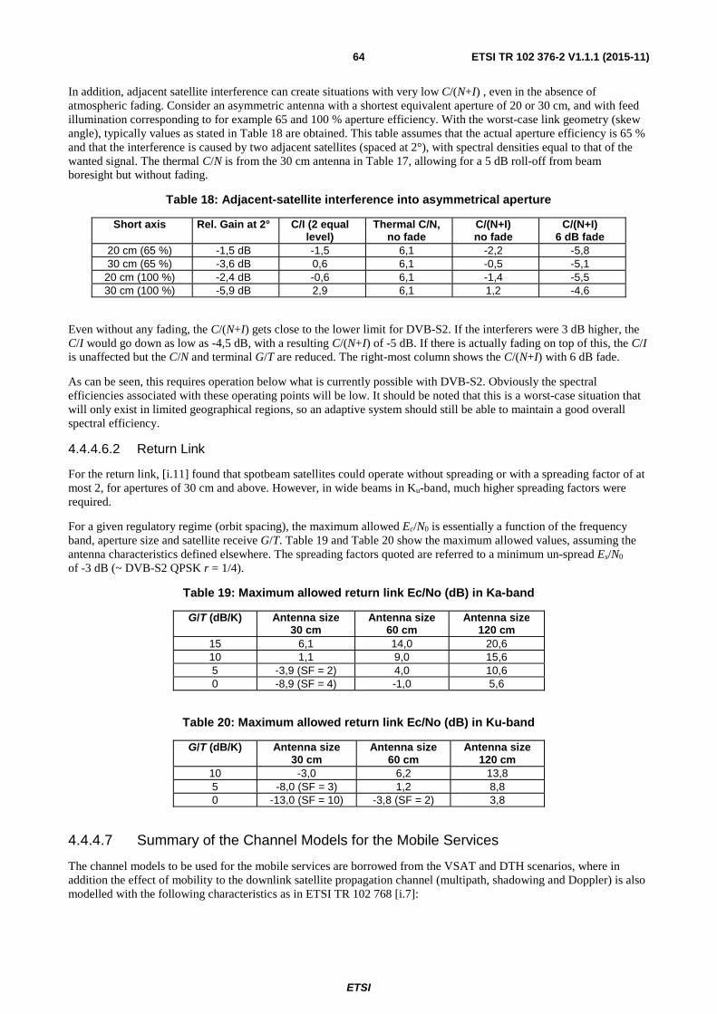
ETSI

ETSI TR 102 376-2 V1.1.1 (2015-11)64

In addition, adjacent satellite interference can create situations with very low C/(N+I) , even in the absence of atmospheric fading. Consider an asymmetric antenna with a shortest equivalent aperture of 20 or 30 cm, and with feed illumination corresponding to for example 65 and 100 % aperture efficiency. With the worst-case link geometry (skew angle), typically values as stated in Table 18 are obtained. This table assumes that the actual aperture efficiency is 65 % and that the interference is caused by two adjacent satellites (spaced at 2°), with spectral densities equal to that of the wanted signal. The thermal C/N is from the 30 cm antenna in Table 17, allowing for a 5 dB roll-off from beam boresight but without fading.

Table 18: Adjacent-satellite interference into asymmetrical aperture

Short axis Rel. Gain at 2° C/I (2 equal level)

Thermal C/N, no fade

C/(N+I) no fade

C/(N+I) 6 dB fade

20 cm (65 %) -1,5 dB -1,5 6,1 -2,2 -5,8 30 cm (65 %) -3,6 dB 0,6 6,1 -0,5 -5,1

20 cm (100 %) -2,4 dB -0,6 6,1 -1,4 -5,5 30 cm (100 %) -5,9 dB 2,9 6,1 1,2 -4,6

Even without any fading, the C/(N+I) gets close to the lower limit for DVB-S2. If the interferers were 3 dB higher, the C/I would go down as low as -4,5 dB, with a resulting C/(N+I) of -5 dB. If there is actually fading on top of this, the C/I is unaffected but the C/N and terminal G/T are reduced. The right-most column shows the C/(N+I) with 6 dB fade.

As can be seen, this requires operation below what is currently possible with DVB-S2. Obviously the spectral efficiencies associated with these operating points will be low. It should be noted that this is a worst-case situation that will only exist in limited geographical regions, so an adaptive system should still be able to maintain a good overall spectral efficiency.

4.4.4.6.2 Return Link

For the return link, [i.11] found that spotbeam satellites could operate without spreading or with a spreading factor of at most 2, for apertures of 30 cm and above. However, in wide beams in Ku-band, much higher spreading factors were required.

For a given regulatory regime (orbit spacing), the maximum allowed Ec/N0 is essentially a function of the frequency band, aperture size and satellite receive G/T. Table 19 and Table 20 show the maximum allowed values, assuming the antenna characteristics defined elsewhere. The spreading factors quoted are referred to a minimum un-spread Es/N0 of -3 dB (~ DVB-S2 QPSK r = 1/4).

Table 19: Maximum allowed return link Ec/No (dB) in Ka-band

G/T (dB/K) Antenna size 30 cm

Antenna size 60 cm

Antenna size 120 cm

15 6,1 14,0 20,6 10 1,1 9,0 15,6 5 -3,9 (SF = 2) 4,0 10,6 0 -8,9 (SF = 4) -1,0 5,6

Table 20: Maximum allowed return link Ec/No (dB) in Ku-band

G/T (dB/K) Antenna size 30 cm

Antenna size 60 cm

Antenna size 120 cm

10 -3,0 6,2 13,8 5 -8,0 (SF = 3) 1,2 8,8 0 -13,0 (SF = 10) -3,8 (SF = 2) 3,8

4.4.4.7 Summary of the Channel Models for the Mobile Services

The channel models to be used for the mobile services are borrowed from the VSAT and DTH scenarios, where in addition the effect of mobility to the downlink satellite propagation channel (multipath, shadowing and Doppler) is also modelled with the following characteristics as in ETSI TR 102 768 [i.7]:

ETSI

ETSI TR 102 376-2 V1.1.1 (2015-11)65

Aeronautical applications:

• Line of Sight conditions can be assumed and the channel can be fairly approximated by a AWGN channel for most of the time. Appropriate Doppler to be applied.

Railway applications:

This scenario can be modelled by superimposing this deterministic and (space) periodic fades on a statistical model accounting for unpredictable obstacles.

The characteristics of the deterministic fades are as follows:

• Catenaries: typically attenuation of 2 dB to 3 dB.

• electrical trellises: up to 15 dB or 20 dB attenuation (depending on the geometry and layout of the obstacles and on the orientation of the railway with respect to the position of the satellite): length ~0,5 m, distance between two consecutive trellises ~43 m.

• Bridges: high signal loss for a length between a few meters up to tens of meters -50 m.

• Tunnels: long-term interruptions.

The statistical model accounting for unpredictable obstacles instead is characterized as it follows:

• For Ku-band, the behaviour of the land mobile satellite channel can be modelled using a 3-state (namely LOS, shadowed and blocked states) Markov chain model, where each state is further characterized by a Rice distribution. The transition matrix coefficients and the distribution parameters can be found in [i.13].

• For Ka-band, the behaviour of the land mobile satellite channel can be modelled using a 3-state (namely LOS, shadowed and blocked states) Markov chain model, where each state is further characterized by a Loo distribution. The corresponding parameters can be found in [i.13] and [i.14].

The channel models relevant for the mobile applications are all the ones pertaining to the VSAT scenario, including the specifications of each sub-block characteristics. The only modification to be applied is the presence of "Mobility-induced propagation effects" in the user downlink, which effectively materializes as the addition of a complex multiplier by a time-varying quantity "C(t)". This pictorially depicted in Figure 38 where the channel model for single carrier per TWTA scenario is described an explicatory example.

The complex factor C(t) has different characteristics according to whether the aeronautical or the railway scenario is to be considered:

• For the aeronautical case C(t) reduced to a complex value with constant unit amplitude (to reflect the AWGN simplification of the channel) and a time varying phase which takes into account the Doppler and Doppler rate. In clause 4.4.4.2 a mathematical expression is proposed to model a particular trajectory of the airplane, i.e.:

ttfjetC )(2)( Δ−= π

(7)

where Δf(t) has the expression given in (1).

• For the railway scenario, C(t) is a random variable which takes into account both the deterministic and the unpredictable fades and whose spectrum is such to reflect the appropriate Doppler spread. If the shadowing effects are ignored the C(t) variable can be generated with the block diagram of Figure 39. The characteristics of "Ricean Fading BW filter" depend on the angle between the direction of travel of the train and the LOS to the satellite and can be found in ETSI TR 102 768 [i.7] and its references.

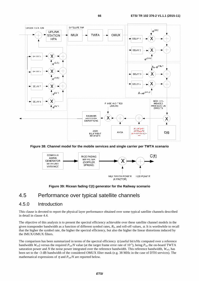
ETSI

ETSI TR 102 376-2 V1.1.1 (2015-11)66

Figure 38: Channel model for the mobile services and single carrier per TWTA scenario

Figure 39: Ricean fading C(t) generator for the Railway scenario

4.5 Performance over typical satellite channels

4.5.0 Introduction

This clause is devoted to report the physical layer performance obtained over some typical satellite channels described in detail in clause 4.4.

The objective of this analysis is to present the spectral efficiency achievable over these satellite channel models in the given transponder bandwidth as a function of different symbol rates, RS, and roll-off values, α. It is worthwhile to recall that the higher the symbol rate, the higher the spectral efficiency, but also the higher the linear distortions induced by the IMUX/OMUX filters.

The comparison has been summarized in terms of the spectral efficiency η (useful bit/s/Hz computed over a reference bandwidth Wref) versus the required Psat/N value (at the target frame error rate of 10-5), being Psat the on-board TWTA saturation power and N the noise power integrated over the reference bandwidth. This reference bandwidth, Wref, has been set to the -3 dB bandwidth of the considered OMUX filter mask (e.g. 38 MHz in the case of DTH services). The mathematical expressions of η and Psat/N are reported below.

SATELLITE TXP

IMUX TWTA OMUX

RECEIVER

AMPLITUDE

DISTORTIONS

ej2 fTt

DELAY 2 X

e-j2 f

Tt

DELAY 3 X

AWGN

ADJACENT

SATELLITE

INTERFERENCE

***

AP1ej2 f

P1t

DELAY 4

AP2e-j2 f

P2t

X

DELAY 1 X

X

PHASE AND FREQ.

ERRORS

UPLINK

STATION

HPA

DELAY 5

DELAY 6

DELAY 7

X

DELAY 8

X

X

X

e-j2 f

Tt

e-j4 f

Tt

ej2 f

Tt

ej4 f

Tt

GROUND STATION

USER

EQUIPMENT

RECEIVER

X

C(t)

MOBILITY-

INDUCED

PROPAGATION

EFFECTS

ETSI

ETSI TR 102 376-2 V1.1.1 (2015-11)67

� = �� ��

����

����

�=� × OBO

�� ����

=��

��×

��

����

× OBO =�

��× � × OBO

where �� is the modulation and coding efficiency, i.e. �

= � × log

2. In order to have a significant statistics for such

analysis, several combinations of transmitted DVB-S2X MODCODs, user symbol rates, and roll-off values have been considered.

4.5.1 Reference Receiver Architecture

The frame error rate curves reported in the following clauses have been obtained by implementing the demodulation strategies shown in Figure 40, where the frame synchronization and the carrier frequency acquisition are assumed to be already granted. Essentially, to cope with the satellite channel impairments, these two main techniques have been considered:

• fractionally spaced equalization;

• carrier phase estimation.

Figure 40: Pictorial view of the demodulation strategy

The rationale for the selection of a fractionally spaced equalizer is briefly summarized. As discussed in [i.20], a symbol spaced equalizer is the optimal solution when following a filter matching the channel response. In general, if the channel characteristics are unknown, this technique leads to an equalizer that it is very sensitive to the estimate of the correct sampling time. In addition, it is important to remind that most widely used timing recovery schemes, like the Gardner algorithm or the data-aided correlation technique, may not give optimized timing offset estimate in case of channel affected by strong inter-symbol interference. Thus, a cleaner approach is to adopt a fractionally spaced equalizer (working at twice the symbol rate) whose performance is insensitive to the timing offset [i.20]. The implemented equalizer consists of 42 complex taps, which are updated in a data-aided manner (i.e. over the pilot fields) using the least-mean square (LMS) algorithm [i.20].

As far as the carrier phase estimate is concerned, the adopted technique is the same described in [i.21]. In practice, the carrier phase compensation is computed by linearly interpolating data-aided estimates over consecutive pilot fields. It is worth noting that the pilot fields are also used for the amplitude estimation to provide at the decoder an accurate soft information about the received symbol distance from the reference constellation points [i.21].

4.5.2 Performance in DTH Broadcasting Services

The DTH channel model is discussed in details in clause 4.4.1, while Table 21 summarizes the main parameters to set up the physical layer simulations (see also Figure 4 notes).

Fractionally spaced

equalizer

zkyk

LMS tapsupdate

ek

Phase estim. and interpol.

Powerestim.

PilotDEMUX

@2Rs@Rs

Buffers

Pilot

DEMUX

rlθk

To soft demapper

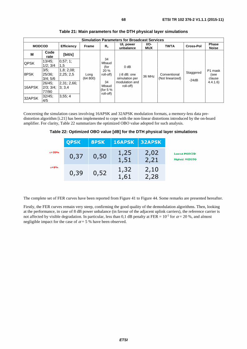
ETSI

ETSI TR 102 376-2 V1.1.1 (2015-11)68

Table 21: Main parameters for the DTH physical layer simulations

Simulation Parameters for Broadcast Services

MODCOD Efficiency Frame Rs UL power unbalance

I/O-MUX TWTA Cross-Pol Phase

Noise

M Code rate [bit/s]

Long (64 800)

34 Mbaud

(for 20 %

roll-off)

34 Mbaud (for 5 % roll-off)

0 dB

(-8 dB: one simulation per

modulation and roll-off)

36 MHz Conventional

(Not linearized)

Staggered

-24dB

P1 mask (see

clause 4.4.1.6)

QPSK 13/45; 1/2; 3/4

0,57; 1; 1,5

8PSK 3/5; 25/36; 3/4; 5/6

1,8; 2,08; 2,25; 2,5

16APSK 26/45; 2/3; 3/4; 77/90

2,31; 2,66; 3; 3,4

32APSK 32/45; 4/5

3,55; 4

Concerning the simulation cases involving 16APSK and 32APSK modulation formats, a memory-less data pre-distortion algorithm [i.21] has been implemented to cope with the non-linear distortions introduced by the on-board amplifier. For clarity, Table 22 summarizes the optimized OBO value adopted for such analysis.

Table 22: Optimized OBO value [dB] for the DTH physical layer simulations

The complete set of FER curves have been reported from Figure 41 to Figure 44. Some remarks are presented hereafter.

Firstly, the FER curves remain very steep, confirming the good quality of the demodulation algorithms. Then, looking at the performance, in case of 8 dB power unbalance (in favour of the adjacent uplink carriers), the reference carrier is not affected by visible degradation. In particular, less than 0,1 dB penalty at FER = 10-5 for α = 20 %, and almost negligible impact for the case of α = 5 % have been observed.

QPSK 8PSK 16APSK 32APSK

0,37 0,501,25

1,51

2,02

2,21

0,39 0,521,32

1,61

2,10

2,28

α=20%

α=5%

Lowest MODCOD

Highest MODCOD

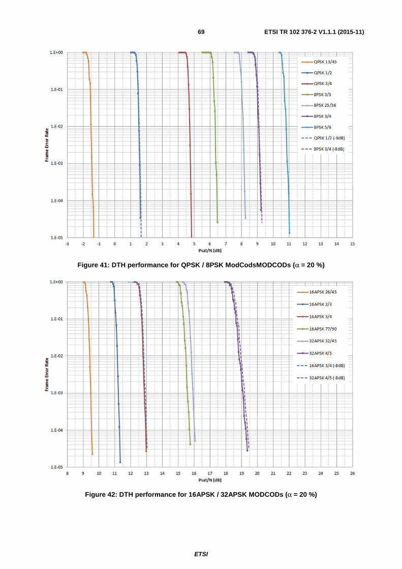
ETSI

ETSI TR 102 376-2 V1.1.1 (2015-11)69

Figure 41: DTH performance for QPSK / 8PSK ModCodsMODCODs (α = 20 %)

Figure 42: DTH performance for 16APSK / 32APSK MODCODs (α = 20 %)

ETSI

ETSI TR 102 376-2 V1.1.1 (2015-11)70

Figure 43: DTH performance for QPSK / 8PSK MODCODs (α = 5 %)

Figure 44: DTH performance for 16APSK / 32APSK MODCODs (α = 5 %)

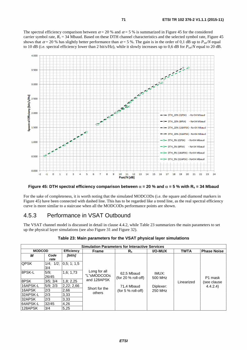
ETSI

ETSI TR 102 376-2 V1.1.1 (2015-11)71

The spectral efficiency comparison between α = 20 % and α = 5 % is summarized in Figure 45 for the considered carrier symbol rate, Rs = 34 Mbaud. Based on these DTH channel characteristics and the selected symbol rate, Figure 45 shows that α = 20 % has slightly better performance than α = 5 %. The gain is in the order of 0,1 dB up to Psat/N equal to 10 dB (i.e. spectral efficiency lower than 2 bit/s/Hz), while it slowly increases up to 0,6 dB for Psat/N equal to 20 dB.

Figure 45: DTH spectral efficiency comparison between α = 20 % and α = 5 % with Rs = 34 Mbaud

For the sake of completeness, it is worth noting that the simulated MODCODs (i.e. the square and diamond markers in Figure 45) have been connected with dashed line. This has to be regarded like a trend line, as the real spectral efficiency curve is more similar to a staircase when all the MODCODs performance points are shown.

4.5.3 Performance in VSAT Outbound

The VSAT channel model is discussed in detail in clause 4.4.2, while Table 23 summarizes the main parameters to set up the physical layer simulations (see also Figure 31 and Figure 32).

Table 23: Main parameters for the VSAT physical layer simulations

Simulation Parameters for Interactive Services MODCOD Efficiency Frame Rs I/O-MUX TWTA Phase Noise

M Code rate

[bit/s]

Long for all "L"sMODCODs and 128APSK

Short for the

others

62,5 Mbaud (for 20 % roll-off)

71,4 Mbaud

(for 5 % roll-off)

IMUX: 500 MHz

Diplexer: 250 MHz

Linearized P1 mask

(see clause 4.4.2.4)

QPSK 1/4; 1/2; 3/4

0,5; 1; 1,5

8PSK-L 5/9; 26/45

1,6; 1,73

8PSK 3/5; 3/4 1,8; 2,25 16APSK-L 5/9; 2/3 2,22; 2,66 16APSK 2/3 2,66 32APSK-L 2/3 3,33 32APSK 2/3 3,33 64APSK-L 32/45 4,26 128APSK 3/4 5,25

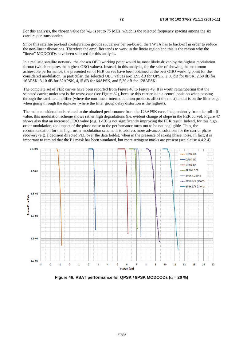
ETSI

ETSI TR 102 376-2 V1.1.1 (2015-11)72

For this analysis, the chosen value for Wref is set to 75 MHz, which is the selected frequency spacing among the six carriers per transponder.

Since this satellite payload configuration groups six carrier per on-board, the TWTA has to back-off in order to reduce the non-linear distortions. Therefore the amplifier tends to work in the linear region and this is the reason why the "linear" MODCODs have been selected for this analysis.

In a realistic satellite network, the chosen OBO working point would be most likely driven by the highest modulation format (which requires the highest OBO values). Instead, in this analysis, for the sake of showing the maximum achievable performance, the presented set of FER curves have been obtained at the best OBO working point for the considered modulation. In particular, the selected OBO values are: 1,95 dB for QPSK, 2,50 dB for 8PSK, 2,60 dB for 16APSK, 3,10 dB for 32APSK, 4,15 dB for 64APSK, and 5,30 dB for 128APSK.

The complete set of FER curves have been reported from Figure 46 to Figure 49. It is worth remembering that the selected carrier under test is the worst-case (see Figure 32), because this carrier is in a central position when passing through the satellite amplifier (where the non-linear intermodulation products affect the most) and it is on the filter edge when going through the diplexer (where the filter group delay distortion is the highest).

The main consideration is related to the obtained performance from the 128APSK case. Independently from the roll-off value, this modulation scheme shows rather high degradations (i.e. evident change of slope in the FER curve). Figure 47 shows also that an increased OBO value (e.g. 1 dB) is not significantly improving the FER result. Indeed, for this high order modulation, the impact of the phase noise to the performance turns out to be not negligible. Thus, the recommendation for this high-order modulation scheme is to address more advanced solutions for the carrier phase recovery (e.g. a decision directed PLL over the data fields), when in the presence of strong phase noise. In fact, it is important to remind that the P1 mask has been simulated, but more stringent masks are present (see clause 4.4.2.4).

Figure 46: VSAT performance for QPSK / 8PSK MODCODs (α = 20 %)

ETSI

ETSI TR 102 376-2 V1.1.1 (2015-11)73

Figure 47: VSAT performance for 16APSK / 32APSK MODCODs (α = 20 %)

Figure 48: VSAT performance for QPSK / 8PSK MODCODs (α = 5 %)

ETSI

ETSI TR 102 376-2 V1.1.1 (2015-11)74

Figure 49: VSAT performance for 16APSK / 32APSK ModCodsMODCODs (α = 5 %)

The spectral efficiency comparison between α = 20 % and α = 5 % is summarized in Figure 50. In this configuration, having assigned the carrier symbol rate on the basis of the "1 + α" rule, it is important to notice the expected gain of α = 5 % with respect to α = 20 % is a function of Psat/N.

Figure 50: VSAT spectral efficiency comparison between α = 20 % and α = 5 %

ETSI

ETSI TR 102 376-2 V1.1.1 (2015-11)75

Figure 51: Qualitative gain of α = 5 % vs. α=20 % in the case of "1 + α "rule

Based on the simulated MODCODs, Figure 51 shows the indicative trend of the spectral efficiency gain of α = 5 % vs. α = 20 %. It is evident that the lower roll-off gain is increasing proportionally to the received power. In addition, for low values of Psat/N, this benefit tends to vanish, becoming even negative. The explanation of that can be easily verified by taking into account that a lower roll-off value implies a smaller Es/N0 (see note) (e.g. -0,58 dB passing from 20 % to 5 %), therefore the achievable spectral efficiency is computed in a lower operating point.

NOTE: It is important to remember that fixing the satellite power and the reference bandwidth, to a lower roll-off corresponds a higher symbol-rate, thus less energy per symbol.

4.5.4 Performance in Broadcast Distribution, Contribution and High Speed IP links

The DSNG channel model is discussed in details in clause 4.4.3, while Table 24 summarizes the main parameters to set up the physical layer simulations (see also Figure 36 and Figure 37).

Table 24: Main parameters for the DSNG physical layer simulations

Simulation Parameters for DSNG/Professional Services MODCOD Efficie

ncy Frame Rs UL power

unbalance I/O-MUX TWTA Cross-Pol Phase

Noise M Code

rate [bit/s]

Long (64 800 bits)

15 Mbaud (for 20 % roll-off)

17 Mbaud

(for 5 % roll-off)

-4 dB 36 MHz Conventional

Staggered -24 dB

P1 mask (see clause 4.4.3.2.4)

8PSK-L 5/9; 26/45

1,6; 1,73

16APSK-L 5/9; 2/3

2,22; 2,66

32APSK-L 2/3 3,33 64APSK 7/9 4,66 128APSK ¾ 5,25 256APSK-L 11/15 5,86

In this configuration, the chosen value for Wref is set to 19 MHz, that is the half value of the DTH case, because two carriers per transponder are assumed.

0 2 4 6 8 10 12 14 16 18 20-3%

-2%

-1%

0

1%

2%

3%

4%

5%

6%

7%

8%

9%

10%

Psat/N [dB]

Spe

ctra

l Effi

cien

cy G

ain:

5%

vs.

20%

ETSI

ETSI TR 102 376-2 V1.1.1 (2015-11)76

Based on the same rationale of the previous channel configuration, VSAT, also in this case the TWTA has to back-off in order to reduce the non-linear distortions. For clarity, the following OBO values have been chosen: 1,25 dB for 8PSK, 2,40 dB for 16APSK, 3,15 dB for 32APSK, 5,65 dB for 64APSK, 7,25 dB for 128APSK, and 9,0 dB for 256APSK.

The complete set of FER curves have been reported in Figure 52 and Figure 53.

Due to the uplink power unbalance set to -4 dB (i.e. the reference carrier power is lower than the adjacent carrier), the 256APSK MODCOD cannot be demodulated, and the 128APSK case shows evident degradation in the FER slope. The impact of this power unbalance, which generates high levels of intermodulation products, is visible in Figure 53. Without power unbalance among the two carriers, these MODCODs perform correctly.

Figure 52: DSNG performance from 8PSK to 128APSK MODCODs (α = 20 %)

ETSI

ETSI TR 102 376-2 V1.1.1 (2015-11)77

Figure 53: DSNG performance from 8PSK to 256APSK MODCODs (α = 5 %)

The spectral efficiency comparison between α = 20 % and α = 5 % is summarized in Figure 54. Again, having assigned the carrier symbol rate on the basis of the "1 + α" rule, the 5 % roll-off value gain follows the same trend explained for the VSAT scenario.

ETSI

ETSI TR 102 376-2 V1.1.1 (2015-11)78

Figure 54: DSNG spectral efficiency comparison between α = 20 % and α = 5 % assuming 4 dB power unbalance among the two carriers

4.6 Channel bonding

4.6.0 Introduction

Channel bonding is a new feature of the S2X system, which is normative for receivers with optional multiple tuners. This means that receiver using a single tuner do not need to consider channel bonding, in fact, cannot be able to decode such signals. However, once multiple tuners are used at receiver side, then channel bonding needs to be supported.

Channel bonding supports bonding of either L = 2 or 3 channels (L being the number of bonded channels).

4.6.1 The principle and advantages of Channel Bonding

The advantages of channel bonding are the following:

For CBR services, there can be cases, where the programs, which are multiplexed inside one channel, do not require the complete channel bandwidth. The remaining bandwidth may not be large enough to multiplex another service, e.g. UHDTV program. However, collecting remaining bandwidths from L transponders may allow multiplexing a complete program into the sum of bandwidths. Thus, channel bonding allows exploiting unused bandwidth.

An example is shown in Figure 55, where the channels of two transponders carry 50 Mbps each. Programs 1, 2, 4, and 5 are transmitted without channel bonding. In the example, the two channels have 10 Mbps as remaining bandwidth, which might be too small to transmit an UHDTV program (assume, 20 Mbps are required for UHDTV). Thus, the TS of program 3 can be transmitted via channel bonding over L = 2 transponders.

The notation "big-Transport-Stream" from ETSI EN 302 307-2 [i.2] specifies the ensemble of packet identifiers (PIDs) from one TS, which will be transmitted via channel bonding. In the example of Figure 55, only the PIDs from program 3 form the "big-Transport-Stream". In principle, all 5 programs in this example could have been grouped together to form the "big-Transport-Stream".

ETSI

ETSI TR 102 376-2 V1.1.1 (2015-11)79

In such cases, where the "big-Transport-Stream" carries a large number of programs, the statistical multiplexing (statmux) gain can be significantly increased, as indicated in Figure 56 (from [i.4]). Assuming that 5 programs (here: "channels") are multiplexed, the statmux gain is about 17 %, allowing for additional 17 Mbps in the above example.

Channel bonding is specified for TS based transmission or for GSE transmission.

Figure 55: Channel bonding use-case: exploiting unused bandwidth

Figure 56: Statmux gain for increasing number of bonded channels (from [i.4])

4.6.2 Channel bonding for TS transmissions

In order to signal to the receiver, how many channels are bonded, on which transponder frequencies they are transmitted and so on, SI tables have to be transmitted on each of the L bonded channels, without using channel bonding. As described above in clause 4.6, the "big-Transport-Stream" consists of all transport streams, which are transmitted over L transponders via channel bonding. The SI tables, which will be duplicated over all bonded transponders, are thus excluded from this "big-Transport-Stream".

In this clause the recommended "useful packet interval" of transponder k, k ∈{1; L}" will be explained.

The throughput rate of this "big-Transport-Stream" is denoted as "total TS rate".

The throughput rate of the k-th transponder, k ∈{1; L}, which is used for channel bonding, is called "TS rate of transponder k".

Figure 57 depicts the details of TS-based channel bonding, however, assumes a useful packet interval, which is not allowed. This setting is used to explain the negative consequences of it. The figure is split into two parts: the upper part shows the data vectors at particular positions in the transmission chain, the lower part shows a block diagram of such transmission chain and explains.

ETSI

ETSI TR 102 376-2 V1.1.1 (2015-11)80

The "big Transport Stream" is the input to a SPLIT block, indicated by the number 1 in the block diagram. 11 data packets (TS packets) are shown in this example, enumerated by 0 to 10. L = 2 branches (i.e. transponders) are assumed for channel bonding in this example. The SPLIT output is routed to each transmitter branch. The SPLIT output has the same throughput rate as the input, i.e. as the "bit Transport Stream". Thus, Null Packets need to be inserted for the remaining bandwidth of the SPLIT output.

Each branch uses a ISSY counter, which is controlled and synchronized by a master channel (usually, one of the L branches). ISSY fields are appended to each TS packet after the ISSY block, i.e. ISCR time stamps, BUFS, and BUFSTAT information according to ETSI EN 302 307-1 [i.1], clause D.2.

The Null Packet Deletion (NPD) block deletes the Null Packets, which have been inserted by the SPLIT process, and the number of consecutively deleted Null Packets is signalled via "Deleted Null Packet" (DNP), which is appended after the ISSY field. In the example from Figure 57, the SPLIT output for channel ch1 had five Null Packets before TS packet 5, thus the DNP value after NPD is 5 in this case (shown in the data for ch1 at position 3). In case "big-Transport Stream" already included "original Null Packets", such packets are transmitted as useful packets, the corresponding input to the MERGE block at receiver side is Null Packets in all branches. In such a case, the receiver can select any branch, e.g. branch number 1.

After FEC encoding at position 4 in Figure 57, a corresponding BB Frame is depicted for each branch, which starts with a BB Header (BBH), followed by a number of information and LDPC + BCH parity bits. The BB Frame does not necessarily have to comprise an integer number of TS packets (as is illustrated in the Figure 57).

After modulation (MOD), further transmit processing (not shown in the Figure 57), the transmission channel (CH), receiver side processing (not shown in the Figure 57), demodulation (DMD), FEC decoding (FEC), a Null Packet Insertion (NPI) block is used at each branch. According to the DNP, Null Packets are reinserted, as shown at position 5 for channel ch1. The MERGE block at receiver side combines the L channels, and acts as the counterpart of the SPLIT process. Finally, the "big Transport Stream" is output.

Figure 57: TS-based Channel Bonding. Problem of long Null Packet intervals (this setting is not allowed by ETSI EN 302 307-2 [i.2])

Figure 57 assumed the same data rate on each of the two branches. The SPLIT output indicated by the Figure shows that five consecutive useful packets are routed to each branch, followed by five Null Packets. Figure 58 now explains the negative consequences of such SPLIT process for the NPI buffer.

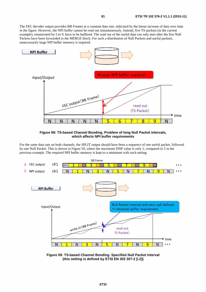
ETSI

ETSI TR 102 376-2 V1.1.1 (2015-11)81

The FEC decoder output provides BB Frames at a constant data rate, indicated by the linear increase of data over time in the figure. However, the NPI buffer cannot be read out instantaneously. Instead, five TS packets (in the current example), enumerated by 5 to 9, have to be buffered. The read out of the useful data can only start after the five Null Packets have been forwarded to the MERGE block. For such a distribution of Null Packets and useful packets, unnecessarily large NPI buffer memory is required.

Figure 58: TS-based Channel Bonding. Problem of long Null Packet intervals, which affects NPI buffer requirements

For the same data rate on both channels, the SPLIT output should have been a sequence of one useful packet, followed by one Null Packet. This is shown in Figure 59, where the maximum DNP value is only 1, compared to 5 in the previous example. The required NPI buffer memory is kept to a minimum with such setting.

Figure 59: TS-based Channel Bonding. Specified Null Packet interval (this setting is defined by ETSI EN 302 307-2 [i.2])

ETSI

ETSI TR 102 376-2 V1.1.1 (2015-11)82

The useful packet intervals are according to the ratio of the total bitrate of the bonded channels to the TS rate of each channel.

For example for L = 2 channels, the useful packet interval of transponder k only takes on only two different values:

floor (total TS rate / TS rate of transponder k) and/or ceil (total TS rate / TS rate of transponder k),

in which floor(x) and ceil(x) denote the flooring and ceiling operation, respectively. The useful packet interval is defined as the number of Null Packets, not including packets with PIDs ∈ {SI tables}, inserted into two useful packets in the SPLIT block plus 1. For the example from Figure 57, the useful packets 4 and 10 are separated by five Null Packet in channel ch0, resulting in a useful packet interval of 6. In the example from Figure 59, the useful packets 1 and 3 are separated by one Null Packet in channel ch1, resulting in a useful packet interval of 2.

NOTE: With the two allowed values for the useful packet interval, any transponder rate can be supported, by using one interval or the other for a certain amount of time.

Another example is shown in Figure 60, where it is assumed that channel ch0 carries 10 Mbps, and channel ch1 20 Mbps. According to the above formula, channel ch0 has a useful packet interval of 3, while channel ch1 may take on the values of 1 or 2. However, for this setting, the useful packet interval of 1 is used for 0 % of the time, while the interval 2 is used for 100 % of the time.

Figure 60: Example for Null Packet intervals

4.6.3 Channel bonding for GSE transmissions

While TS is still the dominant format in most present broadcasting systems, an increasing importance of IP can be observed: many broadcasting receivers already include an IP-stack, satellite re-distribution via SAT-IP is emerging, and other new broadcasting standards become full-IP based. IP transmission can be flexibly realized with the GSE format. Since DVB-S2X introduced GSE-HEW (high efficiency mode), Channel Bonding for GSE can be efficiently realized. Clause 5.1.8.3 of ETSI EN 302 307-2 [i.2] already describes Channel Bonding for GSE in much detail, so only a few notes will be added here.

Channel Bonding for GSE is based on baseband frames (BBFRAMEs), as compared to TS packet-based bonding for the TS case. This is similar as PLP Bundling in DVB-C2 [i.5], described in annex C thereof. Thus, ISCR time stamps are included every BBFRAME ("high efficiency mode"), which reduces the overhead compared to much shorter TS packets ("normal mode"). No Null Packets needed, which allows both the SPLIT process at transmitter side and the MERGE process at receiver side to operate at the rates of the individual channels. These rates are lower than the rate of the "big input TS" in case of TS based bonding, allowing easier implementation.

Clause 5.1.8.3 of ETSI EN 302 307-2 [i.2] further describes Channel Bonding for the cases of Generic Packetized streams, and Generic Continuous streams using GSE. In these cases, ISSY fields are added to every packet, similarly as for TS Channel Bonding.

For channel bonding using Generic Packetized streams (TS/GS = 00), only ISCR_SHORT is allowed. Therefore, the use of this mode is not recommended since timing constraints may not allow correct alignment of packets.

For channel bonding using Generic Continuous streams (TS/GS = 01), the use of ISCR_SHORT is not recommended since timing constraints may not allow correct alignment of packets.

4.7 S2X system configurations The DVB-S2X standard defines five application areas and profiles: Broadcast, Interactive, DSNG, professional and VL-SNR.

ETSI

ETSI TR 102 376-2 V1.1.1 (2015-11)83

Table 25 associates them to the system configurations and mechanisms specified in ETSI EN 302 307-2 [i.2]. All elements in Table 25 are optional in transmitting and receiving equipment complying with the S2 specification ETSI EN 302 307-1 [i.1]. At least "Normative" subsystems and functionalities have to be implemented in the transmitting and receiving equipment to comply with the S2X specification for a specific application area.

Table 25: System Configurations and Application Areas

System configurations Broadcast services

Interactive services

DSNG Professional services

VL-SNR

FECFRAME (normal) (see MODCODs in note 1)

64 800 (bits)

QPSK 1/4,1/3, 2/5 (S2-MODCODs)

N N N N N

1/2, 3/5, 2/3, 3/4, 4/5, 5/6,

8/9, 9/10 (S2-MODCODs)

N N N N N

13/45; N N N N N 9/20; 11/20; N N N N N

8PSK

3/5, 2/3, 3/4, 5/6, 8/9, 9/10 (S2-MODCODs) N N N N N

23/36; 25/36; 13/18 N N N N N 8APSK-L (see note 7) 5/9;26/45 N N N N N 16APSK 2/3, 3/4, 4/5, 5/6, 8/9, 9/10

(S2-MODCODs) N N N N N

26/45; 3/5; 28/45; 23/36; 25/36; 13/18; 7/9; 77/90

N N N N N

16APSK-L (see note 7) 5/9; 8/15; 1/2; 3/5; 2/3 N N N N N 32APSK 3/4, 4/5, 5/6, 8/9, 9/10

(S2-MODCODs) N

N N N N

32/45; 11/15; 7/9; N N N N N 32APSK-L (see note 7) 2/3 N N N N N 64APSK 11/15; 7/9; 4/5; 5/6; O N N N O 64APSK-L (see note 7) 32/45 O N N N O 128APSK 3/4; 7/9 NA O O N NA 256APSK 32/45; 3/4 NA O O N NA 256APSK-L (see note 7)

29/45; 2/3; 31/45; 11/15 NA O O N NA

FECFRAME (short) (see MODCODs in note 1)

16 200 (bits)

QPSK 1/4,1/3, 2/5 (S2-MODCODs)

NA N O N N

1/2, 3/5, 2/3, 3/4, 4/5, 5/6, 8/9

(S2-MODCODs)

NA N O N N

11/45; 4/15; 14/45; 7/15 8/15; 32/45

NA N O N N

8PSK

3/5, 2/3, 3/4, 5/6, 8/9 (S2-MODCODs) NA N O N N

7/15; 8/15; 26/45; 32/45 NA N O N N 16APSK 2/3, 3/4, 4/5, 5/6, 8/9

(S2-MODCODs) NA N O N N

7/15; 8/15; 26/45; 3/5; 32/45 NA N O N N 32APSK 3/4, 4/5, 5/6, 8/9

(S2-MODCODs) NA

N O N N

2/3; 32/45 NA N O N N VL-SNR Header (see MODCODs note 1)

O

O O NA

N

QPSK 2/9 (normal) NA O O NA N BPSK 1/5; 4/15; 1/3 (short)

1/5; 11/45; 1/3 (medium) NA O O NA N

ETSI

ETSI TR 102 376-2 V1.1.1 (2015-11)84

System configurations Broadcast services

Interactive services

DSNG Professional services

VL-SNR

BPSK-S Spreading Factor 2

1/5; 11/45 (short) NA O O NA N

Super-frame NA O O O O Part II PLHEADER (see note 5)

8-bits N N N N N

Extended PLHEADER For Wide-band mode (see note 5)

8 + 8 bits (time slicing) O O NA O O

GSE-High Efficiency Mode

For GSE/GSE-Lite (see note 6)

N N N N N

Roll-off 0,15; 0,10 and 0,05

N N N N N

Channel bonding (see note 2)

N (see note 3)

NA NA O NA

VCM (see note 4)

N N N N N

ACM NA N O O N N = normative, O = optional, NA = not applicable, NOTE 1: Ability to skip VL-SNR frames: Normative. NOTE 2: Requires Input Stream Synchronizer, Null-Packet Deletion and Dummy Frame insertion. NOTE 3: Normative for broadcast services in case of optional multiple tuner receivers. NOTE 4: Any S2X receiver recognizes the whole set of MODCODS within the PLHeader and skip the XFECFrame if the

MODCOD is not supported. NOTE 5: Part II PLHEADER and Extended PLHEADER for wideband transponders (Part I or Part II, annex M) cannot

coexist in the same carrier but either can coexist with the VL-SNR header. NOTE 6: GSE is optional while support for GSE-Lite in GSE-HEM is normative across all the services. NOTE 7: xxx-L = MODCODs optimized for quasi-linear channels.

5 Broadcast applications

5.0 Introduction This clause highlights the main features of DVB-S2X air interface and quantifies the performance gain of DVB-S2X air interface in comparison to the performance of DVB-S2 applied to reference scenario for broadcast applications.

5.1 DVB-S2X features for broadcast applications

5.1.1 Broadcasting with differentiated channel protection

The broadcasting profile of DVB-S2X supports the VCM as a normative feature, which means that within a TDM DVB-S2X carrier, the MODCOD selection may change on a frame by frame basis corresponding to different services. This allows operators to adjust transmission robustness versus efficiency according to the service availability they want to guarantee to the users, and to differentiate services according to the quality of service requirements.

The use of VCM in conjunction with simulcast can be used to guarantee service continuity in the presence of a heavy atmospheric fading, at the same time offering a high quality service in the absence of rain attenuation. By allowing a tolerable degradation in the picture quality during a heavy rain fading (i.e. the use of SD quality instead of HD quality or the use of HD instead of UHD), it is possible to significantly increase the overall system spectral efficiency.

At the receiver, it is assumed that the two streams corresponding to the same content are video decoded independently but the time synchronization between the two streams are maintained such that the output stream for the same content can switch seamlessly between the two frame depending on the fading conditions.

Compared to a scalable video coding with 2 or more layers of coded content, the use of simulcasting of low and high quality streams offers a simpler video coding and decoding solutions and possible a lower overhead (if the required bit rate for the lower quality stream is considerably lower than that of higher quality stream).

In the following clauses, two examples system scenarios are introduced to quantify the potential performance gain of the VCM together with simulcasting (associated with DVB-S2X) compared to DVB-S2.

ETSI

ETSI TR 102 376-2 V1.1.1 (2015-11)85

5.1.2 Channel bonding

The DVB-S2 system was designed to carry a single or multiple MPEG Transport Streams (or generic continuous streams) over a single satellite transponder. The main DTH application in 2003 was HDTV multi-programme delivery using AVC Video coding (H.264), requiring about 10 Mbits/s per program in case of constant bit-rate coding (CBR). Therefore in a single 36 MHz transponder, delivering about 60 Mbits/s in S2 format, it was possible to broadcast 6 HDTV CBR programs, which could be increased to 7 by exploiting the 20 % gain of Statistical Multiplexing (see Figure 56). DVB-S2X system was developed in 2013, when HEVC video coding and UHDTV-1 (four times the definition of HDTV) are becoming a reality. Assuming that an UHDTV-1 signal requires four times the transmission capacity of HDTV for the same compression system, and that HEVC doubles the compression efficiency versus AVC, can be estimated a required bit-rate per UHDTV-1 CBR program of 20 Mbits/s. Under such circumstances, a 60 Mbits/s DVB-S2 signal could provide 3 UHDTV-1 CBR programs per transponder, and the statistical multiplexing gain would be significantly reduced (e.g. 12 % instead of 20 %, assuming Figure 56 is applicable to UHDTV and HEVC), thus not allowing the transmission of an additional program.

In order to increase the statistical multiplexing gain for UHDTV-1, S2X implements "channel bonding", allowing to merge the capacity of two or three transponders to transport a single "big Transport Stream" (Stat-MUX). This functionality is available only for multi-tuner receivers, which are anyway finding their way in the market also to implement other functionalities (e.g. watch one program and record another one, picture-in-picture display).

When the number of bonded transponders (BW = from 33 MHz to 38 MHz) is two, the expected difference in statistical multiplexing gain of S2X over S2 for UHDTV-1 is of the order of 7 %, which would increase to 12 % when there are three bonded channels. In addition, the availability of a "big-TS" allows the spare capacity in individual transponders to be accumulated, accommodating an additional UHDTV-1 program.

It should be noted that the channel bonding in DVB-S2X is only supported when constant coding and modulation (CCM) is used over the transponders (see ETSI EN 302 307-2 [i.2] clause 5.1.8.1).

5.1.3 Higher order modulation

The DVB-S2X supports as normative feature the 16APSK (as well as 32APSK) modulation for broadcasting applications. The use of higher order modulations are particularly advantageous for Ka-band broadcasting system in combination with variable coding and modulation. The use of 16APSK in such scenario would allow a higher spectral efficiency for users in clear sky while the use of more protected MODCODs can ensure achieving the target service availability by allowing a graceful degradation of the service quality.

5.2 Comparative Performance Assessment

5.2.0 Introduction

In order to assess the comparative performance of the DVB-S2X with respect to DVB-S2, two system scenarios are presented here as reference examples for the existing or upcoming satellite broadcasting systems. The first scenario concerns with a single beam broadcast satellite with a wide geographic coverage operating in Ku-band while the second reference scenario deals with a multi-beam broadcasting satellite that provides distinct linguistic coverage over Europe in BSS Ka-band frequency (21,4 to 22,0 GHz).

5.2.1 Receiver architecture assumptions

The performance comparison between the two air interfaces has been carried out using the following categories of receiver technologies:

• DVB-S2 Legacy Receivers: implementing DVB-S2 air interface according the broadcasting profile with a limited capability to tolerate inter-symbol interference due to the bandlimited satellite channel. Such receivers are assumed to operate only in CCM mode with QPSK or 8PSK modulation scheme and no capability of digital channel bonding.

• DVB-S2 Enhanced Receivers: implementing DVB-S2 air interface broadcasting profile (similar to the legacy receivers). Additionally, the enhanced receivers are assumed to be capable of mitigating interference caused by bandlimited channel (e.g. using baseband equalizers) that would allow increasing the symbol rate. It should however be noted that the MODCOD selection is constraint by the broadcasting profile of DVB-S2.

ETSI

ETSI TR 102 376-2 V1.1.1 (2015-11)86

• DVB-S2X Enhanced Receivers: implementing DVB-S2X air interface broadcasting profile and capable of equalizing the linear distortions caused by the bandlimited channel. Such receivers are assumed to support digital channel bonding (up to three BBframes), 16APSK modulation and MODCODSs according to DVB-S2X broadcasting profile.

NOTE: The enhanced receiver architecture similar to that discussed in clause 4.5.1 and illustrated in Figure 40 is considered for the comparative performance analysis. Accordingly, the optimal value of the symbol rate that maximizes the throughput for a typical broadcasting channel is expected to be 34 MBaud (as shown in Table 21).

5.2.2 Video Service Quality

Two classes of video service quality are assumed for this performance analysis:

• High Definition (HD) Quality: to be provided by MPEG-4 CODEC with an average required bit rate of 8 Mbits/sec per stream.

• Ultra High Definition (UHD) Quality: to be provided by HEVC CODEC with an average required bit rate of 20 Mbits/sec per stream.

The target service availability in each scenario is 99,9 % of the time over the entire coverage area. For a DVB-S2 air interface with a constant coding and modulation, this service availability is applied directly to each video stream (HD or UHD).

For DVB-S2X, supporting VCM, the service availability of 99,9 % is provided by two video quality levels associated with each video streams as follows:

• The HD service availability of 99,0 % , complemented by a lower quality stream (MPEG-4 coded at 1,0 Mbits/sec) of the same program with a service availability of 99,9 %.

• The UHD service availability of 99,0 % (or 97,0 %), complemented by a lower quality stream (HEVC coded at 2,0 Mbits/sec) of the same video content with a service availability of 99,9 %.

The higher quality (HQ) and lower quality (LQ) streams are decoded independently but the receiver is assumed to be able to maintain the synchronization between the two streams and switch between the two to maintain the quality and service availability. The overall quality of experience provided by such service is considered acceptable while maintaining a lower link margin and delivering a larger number of TV program channels.

5.2.3 Example Scenario 1: Ku-band broadcasting with a wide coverage

5.2.3.0 Introduction

This example scenario is defined as a broadcasting satellite in Ku-band located at 95 °E geostationary orbit providing broadcasting services to India. The geographical area is selected according to the emerging BSS market focusing on Indian sub-continental coverage. Figure 61 provides the coverage area and the estimated antenna gain.

A total electrical DC power constraint of 5 kW is considered for the broadcasting satellite payload. Such payload can typically accommodate up to 24 transponders each consisting of 120 W TWTA active power amplifiers. A nominal bandwidth of 36 MHz per IMUX/OMUX and the adjacent transponder's central frequency spacing of 40 MHz are assumed for this scenario. Each power amplifier is assumed to operate in single carrier mode.

Figure 62 illustrates examples of percentage of outage time as a function of atmospheric attenuation for two populated locations within the coverage area for this reference scenario (taking into account the orbital location). The computation has been carried out according to Recommendation ITU-R P.618 [i.34]. As shown in Figure 62, a fade margin of 5,1 dB is required to ensure 99,9 % service availability over the entire coverage area. The rain fade margin is reduced to 1,5 dB to ensure 99,0 % service availability.

Considering the on-board antenna gain, the satellite orbital location and the free space signal attenuation, a minimum EIRP of 53,5 dBW in clear sky is assumed over the coverage area.

User terminals with minimum effective dish sizes of 65 cm and G/T of 12,2 dB/K are considered in this analysis.

The interference due to adjacent satellites is assumed to correspond to C/I of 13 dB. Other sources of inter-system interference is assumed negligible.

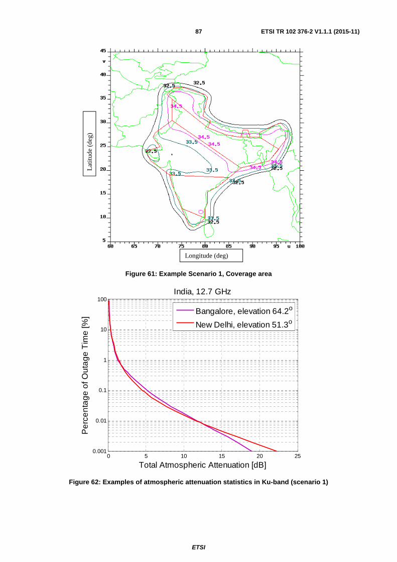
ETSI

ETSI TR 102 376-2 V1.1.1 (2015-11)87

Figure 61: Example Scenario 1, Coverage area

Figure 62: Examples of atmospheric attenuation statistics in Ku-band (scenario 1)

0 5 10 15 20 250.001

0.01

0.1

1

10

100

Total Atmospheric Attenuation [dB]

Pe

rce

nta

ge

of O

uta

ge

Tim

e [%

]

India, 12.7 GHz

Bangalore, elevation 64.2o

New Delhi, elevation 51.3o

Longitude (deg)

Lat

itud

e (d

eg)

ETSI

ETSI TR 102 376-2 V1.1.1 (2015-11)88

5.2.3.1 Study cases for reference scenario 1

5.2.3.1.0 Introduction

Considering system reference scenarios as outlined above, several study cases are defined to establish a benchmark performance according to the existing DVB-S2 solutions as well as enhanced solutions according to DVB-S2 and DVB-S2X specifications. The definition and justification of each study case is outlined below.

5.2.3.1.1 Study case 1.1: DVB-S2 with legacy receiver and MPEG-4 decoder

This study case serves as a benchmark outlining the expected performance of legacy DVB-S2 receivers according to reference scenario 1 assumptions as described above. Considering the transponder bandwidth and the transponder spacing, a symbol rate of 30 MBaud is considered for this study case. The target service in this study case is the broadcasting of HD quality television programs with an average bit rate of 8 Mbits/sec per stream. The target availability for each channel is set to 99,9 %.

5.2.3.1.2 Study case 1.2: DVB-S2 with enhanced receiver and MPEG-4 decoder

Similar assumptions as case 1.1 are considered except for the receiver architecture. In this study case, the receiver remains compliant with DVB-S2 for the DTH profile but it also supports the use of a higher symbol rate without any performance loss compared to the legacy receiver of case 1.1. In particular, the receiver is assumed to be tolerant to Inter-symbol interference caused by bandlimited IMUX/OMUX filters when up to a symbol rate of 34 MBaud (similar channel model as clause 4 is considered). Even though the actual spectral efficiency of the selected MODCOD could be similar or lower than that of Case 1.1, the overall throughput is expected to be higher due to the use of a higher symbol rate.

5.2.3.1.3 Study case 1.3: DVB-S2X with enhanced receiver and MPEG-4 decoder

This study case examines the use of DVB-S2X together with an enhanced receiver and MPEG-4 video decoder to deliver HD quality TV programs. A service availability of 99,0 % for the HD quality streams is targeted. Each HD quality stream is complemented by a lower quality MPEG-4 compressed stream of the same content to ensure 99,9 % availability of service. The two parallel streams coexist as a simulcast over the same transponder. Although the two streams are decoded independently, it is assumed that the receiver is capable of synchronizing the two streams and switch from a higher quality to a lower quality stream in case of detected error. This is to ensure the continuity of service in a fading condition and the capability of reverting to the high quality stream in a normal channel condition.

In this study case, the digital bonding feature of DVB-S2X is NOT used since the VCM transmission is considered.

5.2.3.1.4 Study case 1.4: DVB-S2 with enhanced receiver and HEVC decoder

This study case is similar to Case 1.2 except for the use of HEVC video encoding to deliver UHD quality service. The service availability of 99,9 % is considered.

5.2.3.1.5 Study case 1.5: DVB-S2X with enhanced receiver and MPEG-4 decoder

This study case is similar to Case 1.3 except for the use of HEVC compression to deliver UHD quality service. The service availability of 99,0 % is considered for the UHD video content with an average bit rate of 20 Mbits/sec complemented by simulcasting of HD quality of the same content at much lower bit rate (2 Mbits/sec) and service availability of 99,9 %.

A summary of study case definition is provided in Table 26.

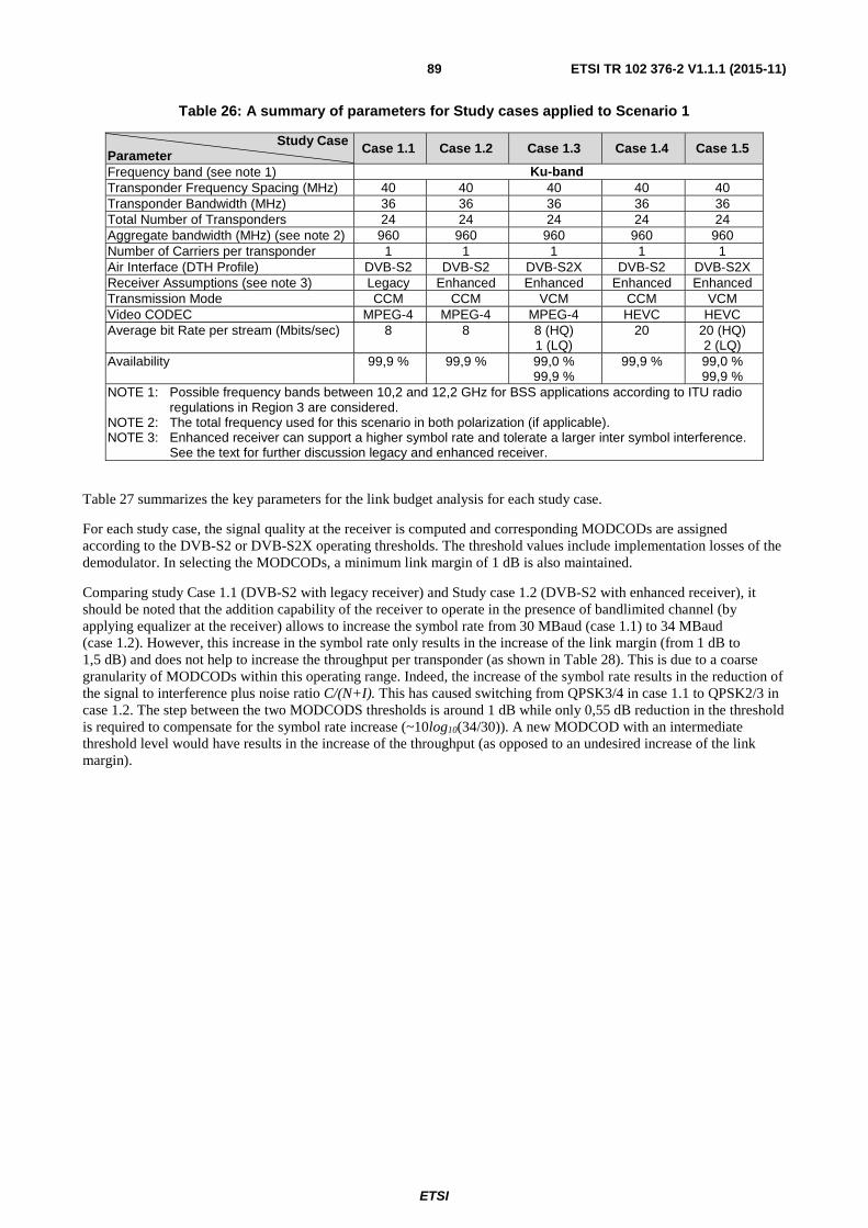
ETSI

ETSI TR 102 376-2 V1.1.1 (2015-11)89

Table 26: A summary of parameters for Study cases applied to Scenario 1

Study Case Parameter Case 1.1 Case 1.2 Case 1.3 Case 1.4 Case 1.5

Frequency band (see note 1) Ku-band Transponder Frequency Spacing (MHz) 40 40 40 40 40 Transponder Bandwidth (MHz) 36 36 36 36 36 Total Number of Transponders 24 24 24 24 24 Aggregate bandwidth (MHz) (see note 2) 960 960 960 960 960 Number of Carriers per transponder 1 1 1 1 1 Air Interface (DTH Profile) DVB-S2 DVB-S2 DVB-S2X DVB-S2 DVB-S2X Receiver Assumptions (see note 3) Legacy Enhanced Enhanced Enhanced Enhanced Transmission Mode CCM CCM VCM CCM VCM Video CODEC MPEG-4 MPEG-4 MPEG-4 HEVC HEVC Average bit Rate per stream (Mbits/sec) 8 8 8 (HQ)

1 (LQ) 20 20 (HQ)

2 (LQ) Availability 99,9 % 99,9 % 99,0 %

99,9 % 99,9 % 99,0 %

99,9 % NOTE 1: Possible frequency bands between 10,2 and 12,2 GHz for BSS applications according to ITU radio

regulations in Region 3 are considered. NOTE 2: The total frequency used for this scenario in both polarization (if applicable). NOTE 3: Enhanced receiver can support a higher symbol rate and tolerate a larger inter symbol interference.

See the text for further discussion legacy and enhanced receiver.

Table 27 summarizes the key parameters for the link budget analysis for each study case.

For each study case, the signal quality at the receiver is computed and corresponding MODCODs are assigned according to the DVB-S2 or DVB-S2X operating thresholds. The threshold values include implementation losses of the demodulator. In selecting the MODCODs, a minimum link margin of 1 dB is also maintained.

Comparing study Case 1.1 (DVB-S2 with legacy receiver) and Study case 1.2 (DVB-S2 with enhanced receiver), it should be noted that the addition capability of the receiver to operate in the presence of bandlimited channel (by applying equalizer at the receiver) allows to increase the symbol rate from 30 MBaud (case 1.1) to 34 MBaud (case 1.2). However, this increase in the symbol rate only results in the increase of the link margin (from 1 dB to 1,5 dB) and does not help to increase the throughput per transponder (as shown in Table 28). This is due to a coarse granularity of MODCODs within this operating range. Indeed, the increase of the symbol rate results in the reduction of the signal to interference plus noise ratio C/(N+I). This has caused switching from QPSK3/4 in case 1.1 to QPSK2/3 in case 1.2. The step between the two MODCODS thresholds is around 1 dB while only 0,55 dB reduction in the threshold is required to compensate for the symbol rate increase (~10log10(34/30)). A new MODCOD with an intermediate threshold level would have results in the increase of the throughput (as opposed to an undesired increase of the link margin).

ETSI

ETSI TR 102 376-2 V1.1.1 (2015-11)90

Table 27: A summary of key link budget parameters for Scenario 1

Study Case Link budget parameters Case 1.1 Case 1.2 Case 1.3 Case 1.4 Case 1.5

EIRP at Saturation (dBW) (see note 1) 53,5 53,5 53,5 53,5 53,5 OBO (dB) (see note 2) 0,3 0,3 0,5 0,3 0,5 Fade Margin for 99,9 % availability (dB) 5,1 5,1 5,1 5,1 5,1 Fade Margin for 99,0 % availability (dB) N/A N/A N/A N/A 1,5 User Terminal minimum antenna size (cm) 65 65 65 65 65 Terminal G/T (dB/K) for 99,9 % availability (5,1 dB atmospheric loss)

12,1 12,1 12,1 12,1 12,1

Terminal G/T (dB/K) for 99,0 % availability (1,5 dB atmospheric loss)

N/A N/A N/A N/A 12,9

C/N0 (dBHz) for 99,9 % of time 81,1 81,1 81,1 81,1 81,1 C/N0 (dBHz) for 99,0 % of time 85,2 85,2 85,2 85,2 85,2 Adjacent Satellite C/I (dB) 13 13 13 13 13 C/(N+I) (dB) for 99,9 % of the time 5,6 5,6 5,6 5,6 5,6 C/(N+I) (dB) for 99,0 % of the time N/A N/A N/A N/A 7,1 Baud Rate (MBaud) 30 34 34 34 34 Required Threshold (dB) 4,6 3,6 3,6 (LQ)

6,6 (HQ) 3,6 3,6 (LQ)

6,6 (HQ) Link Margin (dB) (see note 3) 1,0 1,5 1,5 1,5 1,5 MODCODs QPSK 3/4 QPSK 2/3 QPSK 2/3 (LQ)

8PSK 3/5 (HQ) QPSK 2/3 QPSK 2/3 (LQ)

8PSK 3/5 (HQ)

NOTE 1: EIRP is computed for continuous wave and the power amplifier operating at saturation (zero input back-off).

NOTE 2: The Output back-off is computed according to QPSK modulation scheme except for Case 1.5 where the combination of QPSK and 8PSK modulation is used per transponder.

NOTE 3: A minimum link margin of 1 dB is assumed in this link budget analysis.

5.2.3.2 Comparative performance results for reference scenario 1

Table 28 presents a summary of the performance results for cases studied under example scenario 1. For each case, the effective bit rate per transponder as well as the total number of video channels delivered by the broadcasting satellite in this example scenario is reported. It is noted that:

• The use of DVB-S2 enhanced receiver for this example scenario does not offer any improvement in terms of the number channels and the throughput. The enhanced receiver in this case will only contribute to higher link margin (as discussed in the previous clause).

• The use of DVB-S2X enhanced receiver with HD video quality (case 1.3) offers 17 % increase in the number of channels due to the use of VCM together with simulcasting (no channel bonding applied).

• The use of DVB-S2X enhanced receiver with UHD video quality (case 1.5) offers 50 % increase in the number of UHD channels compared to that of DVB-S2 with enhanced receivers (case 1.4) due to the use of VCM and simulcasting (no channel bonding applied).

ETSI

ETSI TR 102 376-2 V1.1.1 (2015-11)91

Table 28: A summary of performance results

Study Case Parameter Case 1.1 Case 1.2 Case 1.3 Case 1.4 Case 1.5

Transponder IMUX/OMUX Bandwidth (MHz)

36 36 36 36 36

Total Number of Transponders 24 24 24 24 24 Symbol Rate (MBaud) 30 34 34 34 34 Air Interface (DTH Profile) DVB-S2 DVB-S2 DVB-S2X DVB-S2 DVB-S2X Receiver Assumption Legacy Enhanced Enhanced Enhanced Enhanced Transmission Mode CCM CCM VCM CCM VCM Average bit rate per video stream (Mbits/sec)

8 8 8 (HQ) 1 (LQ)

20 20 (HQ) 2 (LQ)

Assigned MODCODs QPSK 3/4 QPSK 2/3 8PSK3/5 (HQ) QPSK 2/3 (LQ)

QPSK 2/3 8PSK (HQ) QPSK 2/3 (LQ)

Effective bit rate per transponder (Mbits/sec) 45,2 45,2 58,7 45,2 59,2

Digital Bonding (see note 1) N/A N/A No N/A No Fractional number of video streams per transponder (see note 2) 5,6 5,6 6,54 2,26 2,86

Statistical multiplexing gain 17 % 17 % 20 % 8 % 8 % Effective number of video streams per transponder (see note 3) 6 6 7 2 3

Total number of video streams (TV channels) delivered by the satellite 6 × 24 = 144 6 × 24 =

144 7 × 24 = 168 2 × 24 = 48 3 × 24 = 72

NOTE 1: For DVB-S2X, the digital bonding can be applied to up to 3 transponders. NOTE 2: This ratio does not include the statistical multiplexing gain. NOTE 3: For DVB-S2X, the effective number of video streams is computed for 3 transponders to take into account

the digital bonding.

5.2.4 Example Scenario 2: Ka-band Multi-Beam broadcasting satellite

5.2.4.0 General

This example scenario concerns with a broadcasting satellite system in BSS Ka-band frequencies (21,4 to 22,0 GHz). The satellite is assumed at 10 °E geostationary orbit providing broadcasting services to eight linguistic beams covering Europe as shown in Figure 63. The frequency plan associated with 8 beams is defined according to a 4 colour scheme as shown in Figure 64. Each beam consists of 5 carriers with a total bandwidth of 300 MHz.

As a benchmark, a Ku-band broadcasting satellite at the same geostationary orbit with similar DC power envelope of 15 kW is considered. The 15 kW DC power envelope typically allows to accommodate up to 64 Ku-band transponders, each with a 120 W TWTA power amplifier.

The Ka-band satellite payload is assumed to have 40 active Ka-band transponders (5 transponders per beam) with single carrier per transponder. The TWTA power amplifier per transponder is assumed to radiate 200 W power at the peak. A nominal bandwidth of 54 MHz per IMUX/OMUX filters and an adjacent frequency spacing of 60 MHz between transponders are assumed.

Figure 65 shows two examples of outage probability as function of atmospheric attenuation for geographical locations within the coverage area. The atmospheric attenuation is computed according to Recommendation ITU-R P.618 [i.34].

ETSI

ETSI TR 102 376-2 V1.1.1 (2015-11)92

Figure 63: Broadcasting satellite with 8 linguistic beams in BSS Ka-band

Figure 64: Frequency Plan - Multi-beam Ka-band Example Scenario 2

Figure 65: Examples of atmospheric attenuation statistics in Ka-band (scenario 2)

0 5 10 15 20 250.01

0.1

1

10

100

Total Atmospheric Attenuation [dB]

Per

cen

tage

of O

uta

ge

Tim

e [%

]

Ka-Band (22 GHz), Sat Lon 10° E

HelsinkiBarcelona

ETSI

ETSI TR 102 376-2 V1.1.1 (2015-11)93

5.2.4.1 Study cases for reference scenario 2

5.2.4.1.0 Introduction

Considering system reference scenarios as outlined for example scenario 2, several study cases are defined to establish a benchmark performance according to the existing DVB-S2 solutions as well as enhanced solutions according to DVB-S2 and DVB-S2X specifications. The definition and justification of each study case is outlined below. A summary of key parameters associated to the each study case is provided in Table 29.

5.2.4.1.1 Study case 2.1: Ku-band reference system with DVB-S2 and legacy receiver

This study case serves as a benchmark, outlining the expected performance of legacy DVB-S2 receivers in a conventional Ku-band system with a single beam and wide coverage over Europe using a broadcasting satellite with an envelope DC power of 15 kW. The payload consists of 64 transponders in Ku-band. Considering the transponder bandwidth and the transponder spacing, a baud rate of 30 MBaud is considered for this study case. The target service case is the broadcasting of UHD quality television channels with an average rate of 20 Mbits/sec per channel. The target availability for each channel is 99,9 %.

5.2.4.1.2 Study case 2.2: Ku-band reference system with DVB-S2 and enhanced receiver

Similar assumptions as case 2.1 is considered here except for the receiver capability of mitigating inter-symbol interference. In this case, the receiver remains compliant with DVB-S2 protocol according to the broadcasting profile while allowing for the optimization of the symbol rate. In particular, the receiver is assumed to be resilient to inter- symbol interference caused by IMUX/OMUX filters.

5.2.4.1.3 Study case 2.3: Ku-band reference system with DVB-S2X with channel bonding

In this study case, DVB-S2X receivers with channel bonding and CCM transmission mode is considered. Similar to Case 2.1 and 2.2 , UHD video quality with 99,9 % service availability is assumed.

5.2.4.1.4 Study case 2.4: Ka-band system with DVB-S2 and enhanced receiver

This study case examines the use of DVB-S2 together with an enhanced receiver and HEVC video decoder to deliver UHD video quality content to the end users in Ka-band multi-beam broadcasting satellite system. A service availability of 99,9 % is targeted. The DVB-S2 receiver in this case operates in CCM transmission mode.

5.2.4.1.5 Study case 2.5: Ka-band system with DVB-S2X

This case examines the use of DVB-S2X air interface and enhanced receiver that supports VCM in broadcasting profile. The receiver is equipped with HEVC decoder to receiver two classes of video qualities; UHD at 99,0 % service availability and a lower quality video HEVC coded at 2 Mbits/sec to complement the UHD stream at 99,9 % service availability.

5.2.4.1.6 Study case 2.6: Ka-band system with DVB-S2X and 97,0 % UHD availability

This study case is similar to Case 2.5 except for the service availability of the UHD quality TV program that is relaxed to 97,0 %.

ETSI

ETSI TR 102 376-2 V1.1.1 (2015-11)94

Table 29: A summary of parameters for Study cases applied to Scenario 2

Study Case Parameter Case 2.1 Case 2.2 Case 2.3 Case 2.4 Case 2.5 Case 2.6

Scenario (see note 1) Ku-band benchmark Ka-band Multi-beam Transponder Frequency Spacing (MHz) 40 40 40 60 60 60 Transponder Bandwidth (MHz) 36 36 36 54 54 54 Total Number of Transponders 64 64 64 40 40 40 Aggregate bandwidth (MHz) (see note 2)

2 560 2 560 2 560 2 400 2 400 2 400

Number of Carriers per transponder 1 1 1 1 1 1 Air Interface (DTH Profile) DVB-S2 DVB-S2 DVB-S2X DVB-S2 DVB-S2X DVB-S2X Receiver Assumptions (see note 3) Legacy Enhanced Enhanced Enhanced Enhanced Enhanced Transmission Mode CCM CCM CCM CCM VCM VCM Video CODEC HEVC HEVC HEVC HEVC HEVC HEVC Average bit Rate per stream (Mbits/sec) 20 20 20 20

20 (HQ) 2 (LQ)

20 (HQ) 2 (LQ)

Availability 99,9 % 99,9 % 99,9 % 99,9 % 99,0 % 99,9 %

97,0 % 99,9 %

NOTE 1: Ku-band frequency between 10,2 GHz and 12,2 GHz for BSS applications according to ITU radio regulations in Region 2 are considered. For multi-beam Ka-band system, the Ka BSS frequency band 21,4 GHz to 22,0 = GHz in both polarizations is considered.

NOTE 2: The total frequency used for this scenario in both polarization (if applicable) and frequency re-use factor 2 (8 beams and 4 colour frequency reuse).

NOTE 3: An enhanced receiver can support a higher symbol rate and tolerate a larger inter symbol interference. See the text for further discussion legacy and enhanced receiver.

ETSI

ETSI TR 102 376-2 V1.1.1 (2015-11)95

Table 30: A summary of key link budget parameters for Scenario 2

Study Case Link budget parameters Case 2.1 Case 2.2 Case 2.3 Case 2.4 Case 2.5 Case 2.6

Scenario Ku-band benchmark Ka-band Multi-beam EIRP at Saturation (dBW) (see note 1) 53.5 53.5 60.7 60.7 60.7 60.7

OBO (dB) (see note 2) 0.5 0.3 0.3 0.3 0.5 1.5

Fade Margin for 99,9 % availability (dB) 3 3 3 9.4 9.4 9.4

Fade Margin for 99,0 % availability (dB) N/A N/A N/A N/A 3.4 N/A

Fade Margin for 97,0 % availability (dB) N/A N/A N/A N/A N/A 2.2

User Terminal minimum antenna size (cm)

65 65 65 65 65 65

Terminal G/T (dB/K) for 99,9 % of the time

12,7 12,7 15,5 15,5 15,5 15,5

Terminal G/T (dB/K) for 99,0 % of the time

N/A N/A N/A N/A 15,7 N/A

Terminal G/T (dB/K) for 97,0 % of the time

N/A N/A N/A N/A N/A 16,2

C/N0 (dBHz) for 99,9 % of time 83,7 83,7 83,7 82,5 82,5 82,5 C/N0 (dBHz) for 99,0 % of time N/A N/A N/A N/A 87,5 N/A

C/N0 (dBHz) for 97,0 % of time N/A N/A N/A N/A N/A 89,3

Adjacent Satellite C/I (dB) 13 13 13 22 22 22

Co-Channel Interference (dB) (see note 3)

N/A N/A N/A 20 20 20

C/(N+I) (dB) for 99,9 % of the time 7,7 7,1 7,1 5,2 5,1 4,1

C/(N+I) (dB) for 99,0 % of the time N/A N/A N/A N/A 10,5 N/A

C/(N+I) (dB) for 97,0 % of the time N/A N/A N/A N/A N/A 11,1

Baud Rate (MBaud) 30 34 34 51 51 51

MODCODs 8PSK3/5 QPSK 5/6 QPSK 5/6 QPSK 2/3 8PSK 5/6 (HQ)

QPSK 2/3 (LQ)

16APSK 2/3 (HQ)

QPSK 3/5 (LQ)

Required Threshold (dB) 6,6 5,7 5,7 3,6 10,4 (HQ) 3,6 (LQ)

10,8 (HQ) 2,8 (LQ)

Link Margin (dB) (see note 4) 1,1 1,4 1,4 1,6 1,5 1,3

NOTE 1: EIRP is computed for continuous wave and the power amplifier operating at saturation (zero input back-off).

NOTE 2 The Output back-off is computed according to the modulation scheme assigned to the transponder in each case. See Table 22 for the selected OBO values per modulation.

NOTE 3: Due to multi-beam co-channel interference. NOTE 4: The link margin is only reported for the Lower Quality stream in case of DVB-S2X. For a higher quality

mode, no excessive margin is required since the system can switch to lower quality mode. A minimum of 1,0 dB link margin is maintained in the link budget analysis.

5.2.4.2 Comparative performance results for reference scenario 2

Table 31 presents a summary of the performance results for cases studied under example scenario 2. For each case, the effective bit rate per transponder as well as the total number of video channels delivered by the broadcasting satellite in this example scenario is reported.

It can be noted that:

• The use of DVB-S2 enhanced receivers (case 2.2), compared to the legacy receivers (case 2.1), do not offer any improvement in terms of the number UHDTV channels and only provide a marginal improvement (4 %) in terms of the throughput per transponder.

• DVB-S2X channel bonding used in the Ku-band (case 2.3) offers around 11 % increase in the number of UHDTV channels compared to DVB-S2 (case 2.2).

• The use of DVB-S2 enhanced receiver with UHD video quality in Ka-band (case 2.4) shows a significant reduction (37%) in the number of video streams compared to a Ku-band broadcasting satellite with the same 15 kW DC power envelope (case 2.2).

• The use of DVB-S2X enhanced receiver with UHD video quality in Ka-band can offer a significant increase in the number of channels compared to DVB-S2 in Ka-band. The increase in the number of UHD channels is around 100 % (case 2.5 or case 2.6 ) compared to DVB-S2 (case 2.4).

ETSI

ETSI TR 102 376-2 V1.1.1 (2015-11)96

Table 31: A summary of performance results - Scenario 2

Study Case Parameter Case 2.1 Case 2.2 Case 2.3 Case 2.4 Case 2.5 Case 2.6

Scenario Ku-band benchmark Ka-band Multi-beam Transponder IMUX/OMUX Bandwidth

(MHz) 36 36 36 60 60 60

Total Number of Transponders 64 64 64 40 40 40 Symbol Rate (MBaud) 30 34 34 54 54 54 Air Interface (DTH Profile) DVB-S2 DVB-S2 DVB-S2X DVB-S2 DVB-S2X DVB-S2X Receiver Assumption Legacy Enhanced Enhanced Enhanced Enhanced Enhanced Transmission Mode CCM CCM CCM CCM VCM VCM Average bit rate per video stream (Mbits/sec) 20 20 20 20 20 (HQ)

2 (LQ) 20 (HQ) 2 (LQ)

Assigned MODCODs 8PSK 3/5 QPSK 5/6 QPSK 5/6 QPSK 2/3 8PSK 5/6 (HQ)

QPSK 2/3 (LQ)

16APSK 2/3 (HQ)

QPSK 3/5 (LQ)

Effective bit rate per transponder (Mbits/sec) 54,3 56,5 56,5 67,9 118,1 122,4

Digital Bonding (see note 1) N/A N/A Yes N/A No No Fractional number of video streams per transponder (see note 2) 2,7 2,8 2,8 3,4 5,4 5,6

Statistical multiplexing gain 8 % 8 % 23 % 12 % 16 % 16 % Effective number of video streams per transponder 3 3 10/3

(see note 3) 3 6 6

Total number of video streams (TV channels) delivered by the satellite

64 x 3 = 192 64x3 = 192 64 x 10/3 ~

213 40 x 3 =

120 40 x 6 =

240 40 x 6 =

240 NOTE 1: For DVB-S2X (CCM), the channel bonding can be applied to up to 3 transponders. NOTE 2: This ratio does not include the statistical multiplexing gain. NOTE 3: For DVB-S2X CCM, the effective number of video streams is computed for every 3 transponders to take into

account the digital channel bonding gain.

6 Interactive applications

6.0 Introduction Broadband interactive services are optimized when delivered over multi-spot network, thanks to the possibility to re-use many times the available user frequency spectrum for a large number of user beams. Indeed, an increased number of High Throughput Satellite (HTS) are being launched to support this technology.

The new S2X specification foresees new MODCODs, called 'linear' MODCODs (indicated by a '-L' notation in the MODCOD name), which have been optimized for a linear channel and in the presence of phase-noise (see note), thus bringing gains of mixed value (in some cases up to about 1 dB lower SNR for the same spectral efficiency). In addition, a finer granularity of the MODCODs has been introduced, reducing the SNR threshold distances from the 1 dB to 1,5 dB of DVB-S2 to an average of about 0,4 dB to 0,5 dB in S2X thereby reducing the extra system margin of ACM-based systems.

NOTE: See Table H.3 in clause H.8 (S2X Specification).

Finally, as a normative feature, S2X mandates the support of a higher modulation order; 64-APSK, as opposed to the optional 32APSK of DVB-S2. This results in an expected spectral efficiency gain of up to 10 %.

There are higher order modulations also optionally available in DVB-S2X, with modulations up to 256 points, thus further increasing the possible spectral efficiency for systems where the link budget allows operating at a higher SNIR levels.

The Very Low SNR MODCODs can also be optionally used in DVB-S2X allowing operation of broadband networks in regions affected by heavy atmospheric fading, at Ka-band, or operating at higher frequency (e.g. Q/V-band) or equipped with small antenna (even mobile) terminals.

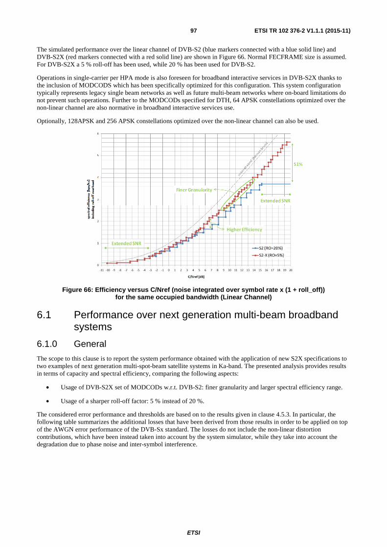
ETSI

ETSI TR 102 376-2 V1.1.1 (2015-11)97

The simulated performance over the linear channel of DVB-S2 (blue markers connected with a blue solid line) and DVB-S2X (red markers connected with a red solid line) are shown in Figure 66. Normal FECFRAME size is assumed. For DVB-S2X a 5 % roll-off has been used, while 20 % has been used for DVB-S2.

Operations in single-carrier per HPA mode is also foreseen for broadband interactive services in DVB-S2X thanks to the inclusion of MODCODS which has been specifically optimized for this configuration. This system configuration typically represents legacy single beam networks as well as future multi-beam networks where on-board limitations do not prevent such operations. Further to the MODCODs specified for DTH, 64 APSK constellations optimized over the non-linear channel are also normative in broadband interactive services use.

Optionally, 128APSK and 256 APSK constellations optimized over the non-linear channel can also be used.

Figure 66: Efficiency versus C/Nref (noise integrated over symbol rate x (1 + roll_off)) for the same occupied bandwidth (Linear Channel)

6.1 Performance over next generation multi-beam broadband systems

6.1.0 General

The scope to this clause is to report the system performance obtained with the application of new S2X specifications to two examples of next generation multi-spot-beam satellite systems in Ka-band. The presented analysis provides results in terms of capacity and spectral efficiency, comparing the following aspects:

• Usage of DVB-S2X set of MODCODs w.r.t. DVB-S2: finer granularity and larger spectral efficiency range.

• Usage of a sharper roll-off factor: 5 % instead of 20 %.

The considered error performance and thresholds are based on to the results given in clause 4.5.3. In particular, the following table summarizes the additional losses that have been derived from those results in order to be applied on top of the AWGN error performance of the DVB-Sx standard. The losses do not include the non-linear distortion contributions, which have been instead taken into account by the system simulator, while they take into account the degradation due to phase noise and inter-symbol interference.

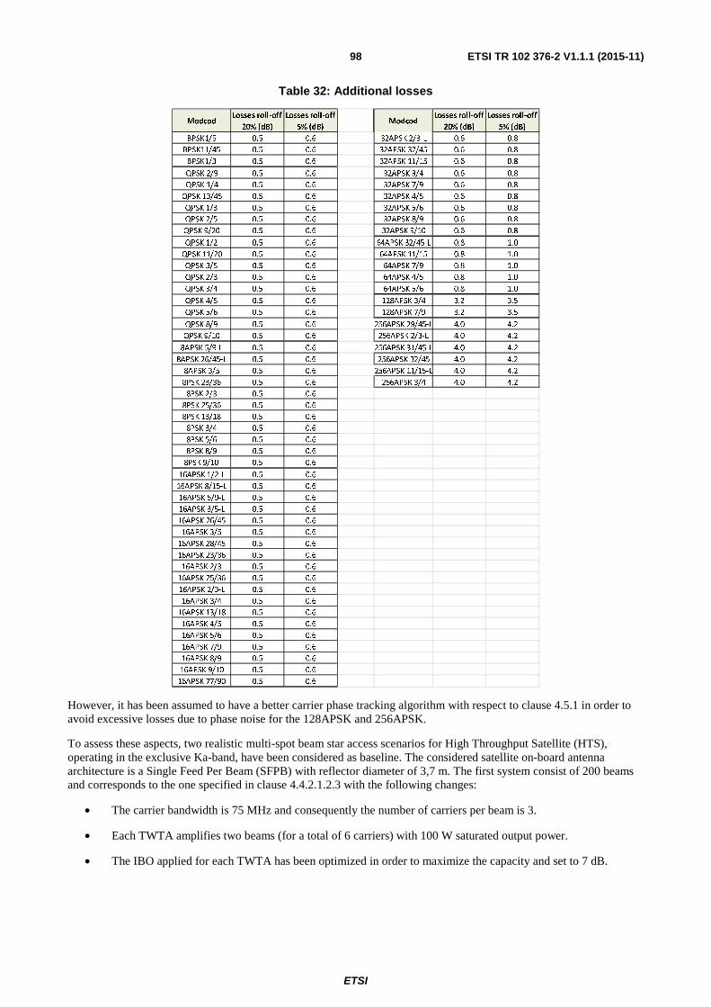
ETSI

ETSI TR 102 376-2 V1.1.1 (2015-11)98

Table 32: Additional losses

However, it has been assumed to have a better carrier phase tracking algorithm with respect to clause 4.5.1 in order to avoid excessive losses due to phase noise for the 128APSK and 256APSK.

To assess these aspects, two realistic multi-spot beam star access scenarios for High Throughput Satellite (HTS), operating in the exclusive Ka-band, have been considered as baseline. The considered satellite on-board antenna architecture is a Single Feed Per Beam (SFPB) with reflector diameter of 3,7 m. The first system consist of 200 beams and corresponds to the one specified in clause 4.4.2.1.2.3 with the following changes:

• The carrier bandwidth is 75 MHz and consequently the number of carriers per beam is 3.

• Each TWTA amplifies two beams (for a total of 6 carriers) with 100 W saturated output power.

• The IBO applied for each TWTA has been optimized in order to maximize the capacity and set to 7 dB.

ModcodLosses roll-off

20% (dB)

Losses roll-off

5% (dB)Modcod

Losses roll-off

20% (dB)

Losses roll-off

5% (dB)

BPSK1/5 0.5 0.6 32APSK 2/3-L 0.6 0.8

BPSK11/45 0.5 0.6 32APSK 32/45 0.6 0.8

BPSK1/3 0.5 0.6 32APSK 11/15 0.6 0.8

QPSK 2/9 0.5 0.6 32APSK 3/4 0.6 0.8

QPSK 1/4 0.5 0.6 32APSK 7/9 0.6 0.8

QPSK 13/45 0.5 0.6 32APSK 4/5 0.6 0.8

QPSK 1/3 0.5 0.6 32APSK 5/6 0.6 0.8

QPSK 2/5 0.5 0.6 32APSK 8/9 0.6 0.8

QPSK 9/20 0.5 0.6 32APSK 9/10 0.6 0.8

QPSK 1/2 0.5 0.6 64APSK 32/45-L 0.8 1.0

QPSK 11/20 0.5 0.6 64APSK 11/15 0.8 1.0

QPSK 3/5 0.5 0.6 64APSK 7/9 0.8 1.0

QPSK 2/3 0.5 0.6 64APSK 4/5 0.8 1.0

QPSK 3/4 0.5 0.6 64APSK 5/6 0.8 1.0

QPSK 4/5 0.5 0.6 128APSK 3/4 3.2 3.5

QPSK 5/6 0.5 0.6 128APSK 7/9 3.2 3.5

QPSK 8/9 0.5 0.6 256APSK 29/45-L 4.0 4.2

QPSK 9/10 0.5 0.6 256APSK 2/3-L 4.0 4.2

8APSK 5/9-L 0.5 0.6 256APSK 31/45-L 4.0 4.2

8APSK 26/45-L 0.5 0.6 256APSK 32/45 4.0 4.2

8APSK 3/5 0.5 0.6 256APSK 11/15-L 4.0 4.2

8PSK 23/36 0.5 0.6 256APSK 3/4 4.0 4.2

8PSK 2/3 0.5 0.6

8PSK 25/36 0.5 0.6

8PSK 13/18 0.5 0.6

8PSK 3/4 0.5 0.6

8PSK 5/6 0.5 0.6

8PSK 8/9 0.5 0.6

8PSK 9/10 0.5 0.6

16APSK 1/2-L 0.5 0.6

16APSK 8/15-L 0.5 0.6

16APSK 5/9-L 0.5 0.6

16APSK 3/5-L 0.5 0.6

16APSK 26/45 0.5 0.6

16APSK 3/5 0.5 0.6

16APSK 28/45 0.5 0.6

16APSK 23/36 0.5 0.6

16APSK 2/3 0.5 0.6

16APSK 25/36 0.5 0.6

16APSK 2/3-L 0.5 0.6

16APSK 3/4 0.5 0.6

16APSK 13/18 0.5 0.6

16APSK 4/5 0.5 0.6

16APSK 5/6 0.5 0.6

16APSK 7/9 0.5 0.6

16APSK 8/9 0.5 0.6

16APSK 9/10 0.5 0.6

16APSK 77/90 0.5 0.6

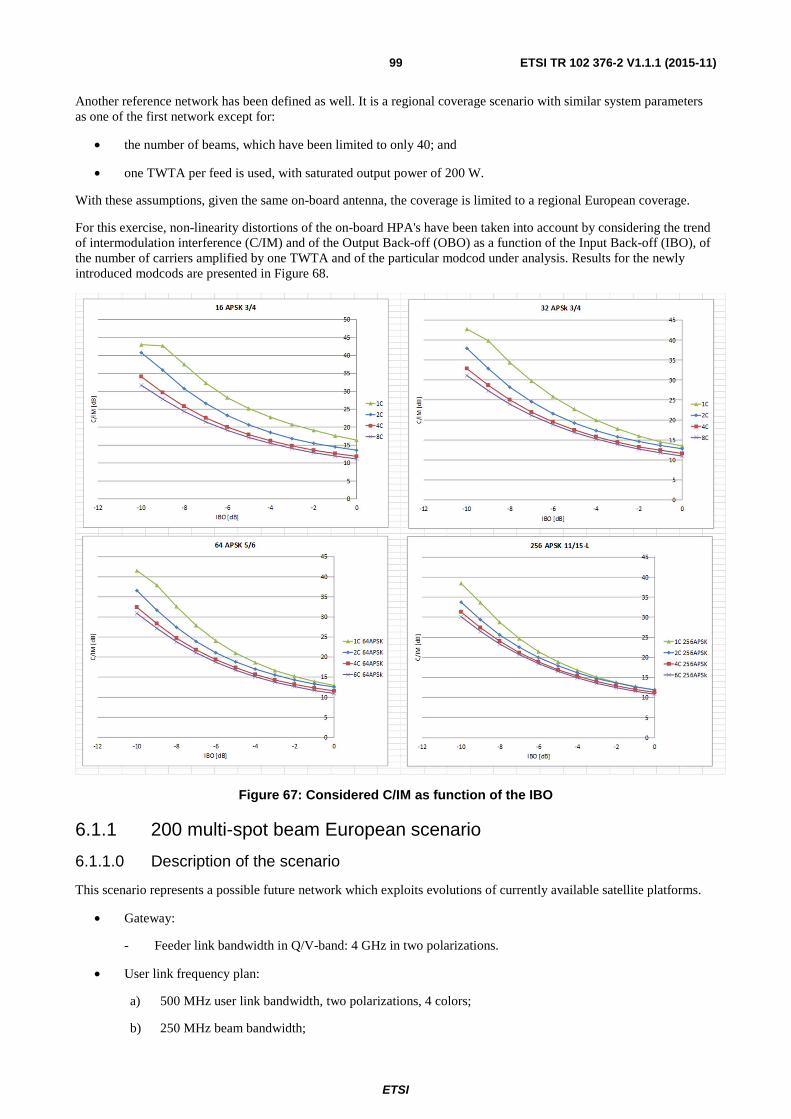
ETSI

ETSI TR 102 376-2 V1.1.1 (2015-11)99

Another reference network has been defined as well. It is a regional coverage scenario with similar system parameters as one of the first network except for:

• the number of beams, which have been limited to only 40; and

• one TWTA per feed is used, with saturated output power of 200 W.

With these assumptions, given the same on-board antenna, the coverage is limited to a regional European coverage.

For this exercise, non-linearity distortions of the on-board HPA's have been taken into account by considering the trend of intermodulation interference (C/IM) and of the Output Back-off (OBO) as a function of the Input Back-off (IBO), of the number of carriers amplified by one TWTA and of the particular modcod under analysis. Results for the newly introduced modcods are presented in Figure 68.

Figure 67: Considered C/IM as function of the IBO

6.1.1 200 multi-spot beam European scenario

6.1.1.0 Description of the scenario

This scenario represents a possible future network which exploits evolutions of currently available satellite platforms.

• Gateway:

- Feeder link bandwidth in Q/V-band: 4 GHz in two polarizations.

• User link frequency plan:

a) 500 MHz user link bandwidth, two polarizations, 4 colors;

b) 250 MHz beam bandwidth;

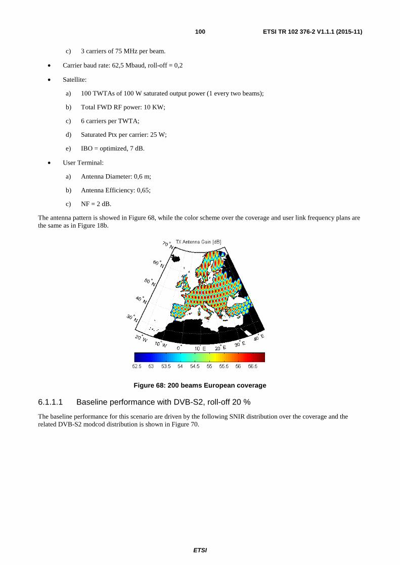
ETSI

ETSI TR 102 376-2 V1.1.1 (2015-11)100

c) 3 carriers of 75 MHz per beam.

• Carrier baud rate: 62,5 Mbaud, roll-off = 0,2

• Satellite:

a) 100 TWTAs of 100 W saturated output power (1 every two beams);

b) Total FWD RF power: 10 KW;

c) 6 carriers per TWTA;

d) Saturated Ptx per carrier: 25 W;

e) IBO = optimized, 7 dB.

• User Terminal:

a) Antenna Diameter: 0,6 m;

b) Antenna Efficiency: 0,65;

c) NF = 2 dB.

The antenna pattern is showed in Figure 68, while the color scheme over the coverage and user link frequency plans are the same as in Figure 18b.

Figure 68: 200 beams European coverage

6.1.1.1 Baseline performance with DVB-S2, roll-off 20 %

The baseline performance for this scenario are driven by the following SNIR distribution over the coverage and the related DVB-S2 modcod distribution is shown in Figure 70.

ETSI

ETSI TR 102 376-2 V1.1.1 (2015-11)101

Figure 69: Baseline 200 beams scenario SNIR Probability Density Function

Figure 70: Baseline 200 beams scenario MODCODs distribution with DVB-S2

As the SNIR PDF analysis shows, the system is equally C/N and C/I limited and the maximum achievable SNIR is around 15 dB. In these conditions, the maximum achievable spectral efficiency is the one of 32APSK 4/5 with a small usage of 32ASPK 5/6.

5 10 15 20 25 30

0.05

0.1

0.15

0.2

0.25

0.3PDF vs Quantized total SNIR dB over the Coverage

SNIR [dB]

PD

F(S

NIR

)

total SNIR

CNDL

CIDL TOT

CIcoch

0

0.05

0.1

0.15

0.2

0.25

0.3

0.35

0.4Traffic weighted modcod PDF vs Modcod index

PD

F(M

odco

d)

QP

SK

1/4

QP

SK

1/3

QP

SK

2/5

QP

SK

1/2

QP

SK

3/5

QP

SK

2/3

QP

SK

3/4

QP

SK

4/5

QP

SK

5/6

8PS

K 3/

5 8P

SK

2/3

8PS

K 3/

416

APS

K 2/

3 16

APS

K 3/

4 16

APS

K 4/

516

APS

K 5/

632

APS

K 3/

416

APS

K 8/

9 32

APS

K 4/

532

APS

K 5/

6

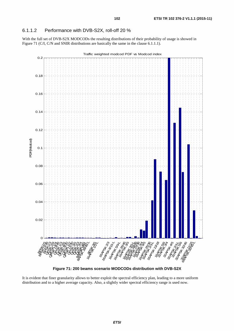
ETSI

ETSI TR 102 376-2 V1.1.1 (2015-11)102

6.1.1.2 Performance with DVB-S2X, roll-off 20 %

With the full set of DVB-S2X MODCODs the resulting distributions of their probability of usage is showed in Figure 71 (C/I, C/N and SNIR distributions are basically the same in the clause 6.1.1.1).

Figure 71: 200 beams scenario MODCODs distribution with DVB-S2X

It is evident that finer granularity allows to better exploit the spectral efficiency plan, leading to a more uniform distribution and to a higher average capacity. Also, a slightly wider spectral efficiency range is used now.

0

0.02

0.04

0.06

0.08

0.1

0.12

0.14

0.16

0.18

0.2Traffic weighted modcod PDF vs Modcod index

PD

F(M

odco

d)

BPS

K1/

5

BPS

K11

/45

BPS

K1/

3Q

PSK

2/9

QPSK

1/4

QPSK

13/4

5Q

PSK

1/3

QPSK

2/5

QPSK

9/20

QPSK

1/2

QPSK

11/2

0Q

PSK

3/5

QPSK

2/3

QPSK

3/4

QPSK

4/5

8APSK

5/9

-L

8APSK

26/

45-L

8PSK

3/5

16AP

SK

1/2-

L

16AP

SK

2/3

16AP

SK

8/15

-L

16AP

SK

5/9-

L

16AP

SK

26/4

5

16AP

SK

3/5

16AP

SK

3/5-

L

16AP

SK

28/4

5

16AP

SK

23/3

6

16AP

SK

3/4

16AP

SK

4/5

16AP

SK

25/3

6

16AP

SK

2/3-

L

16AP

SK

13/1

8

16AP

SK

5/6

32AP

SK

3/4

32AP

SK

4/5

32AP

SK

2/3-

L

32AP

SK

5/6

32AP

SK

32/4

5

32AP

SK

11/1

5

64AP

SK

32/4

5-L

ETSI

ETSI TR 102 376-2 V1.1.1 (2015-11)103

6.1.1.3 Performance with DVB-S2X, roll-off 5 %

By reducing the roll-off, the carrier symbol rate is increased, with the following main two consequences:

• The signal power spectral density (PSD) is now integrated over a larger bandwidth and therefore the C/N distribution (and so the total SNIR) results slightly lower w.r.t. the baseline scenario; this effect is reflected by the MODCOD distribution.

• The overall capacity, proportional to the symbol rate, increases linearly.

With a roll-off of 5 %, a symbol rate of 71,4 Mbaud has been considered.

The following two figures represent these two effects:

Figure 72: 200 beams scenario SNIR probability distribution function with roll-off 5 %

5 10 15 20 25 30

0.05

0.1

0.15

0.2

0.25

0.3PDF vs Quantized total SNIR dB over the Coverage

SNIR [dB]

PD

F(S

NIR

)

total SNIR

SNIRDLCNDL

CIDL TOT

CIcoch

ETSI

ETSI TR 102 376-2 V1.1.1 (2015-11)104

Figure 73: 200 beams scenario MODCODs distribution with DVB-S2X and roll-off 5 %

Table 34 summarizes the overall capacity results for the three cases related to this european scenario.

Table 33: Performance summary and comparison between DVB-S2, DVB-S2X and DVB-S2X with reduced roll-off

The performance improvement resulting from the application of the new set of modcods corresponds to 3,27 % w.r.t. DVB-S2, mainly due to the finer granularity. With the roll-off reduction from 20 % to 5 % instead, the gain in performance rises to 13,2 % with respect to DVB-S2 and to 9,6 % w.r.t. DVB-S2X with 20 % roll-off. The reduction of the SNIR in fact does not penalize significantly the average spectral efficiency (from 3,37 to 3,24 bit/sym), while the increased symbol rate allows for a higher capacity.

6.1.2 40 multi-spot beam regional scenario

6.1.2.0 Description of the scenario

This scenario provides an example of regional system with very high throughput requirements.

• Gateway:

- Feeder link bandwidth in Q/V-band: 4 GHz in two polarizations

0

0.02

0.04

0.06

0.08

0.1

0.12

0.14

0.16

0.18

0.2Traffic weighted modcod PDF vs Modcod index

PD

F(M

odco

d)

BPS

K1/5

BPS

K11/

45BP

SK1

/3Q

PSK

2/9

QP

SK 1

/4Q

PSK

13/4

5Q

PSK

1/3

QP

SK 2

/5Q

PSK

9/20

QP

SK 1

/2

QPS

K 11

/20

QP

SK 3

/5Q

PSK

2/3

QP

SK 3

/4Q

PSK

4/5

8APS

K 5

/9-L

8AP

SK 2

6/45

-L

8PS

K 3/

5

16AP

SK

1/2-

L 16

APSK

2/3

16AP

SK 8

/15-

L

16AP

SK

5/9-

L

16AP

SK

26/4

5

16AP

SK 3

/5

16AP

SK

3/5-

L

16AP

SK

28/4

5

16AP

SK

23/3

6

16AP

SK 3

/4

16AP

SK 4

/5

16AP

SK

25/3

6

16AP

SK

2/3-

L

16AP

SK

13/1

8 16

APSK

5/6

32AP

SK 3

/4

32AP

SK 4

/5

32AP

SK

2/3-

L

32AP

SK 5

/6

32AP

SK

32/4

5

32AP

SK

11/1

5

64AP

SK 3

2/45

-L

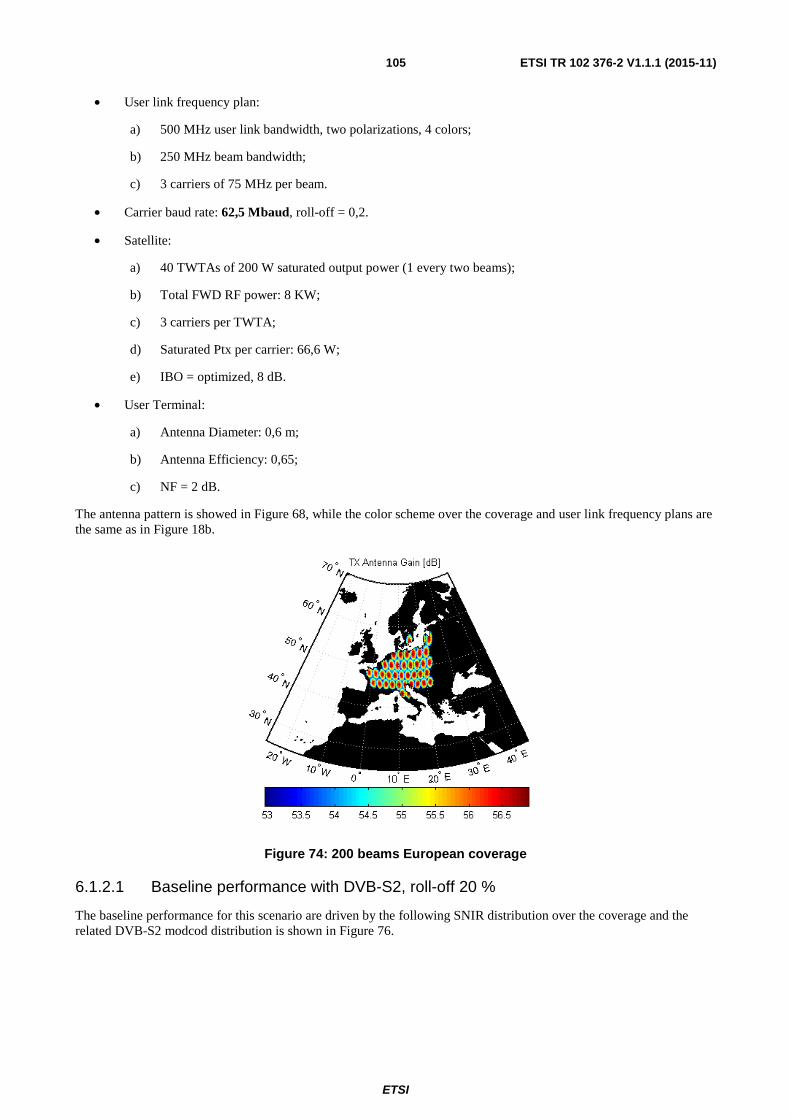
ETSI

ETSI TR 102 376-2 V1.1.1 (2015-11)105

• User link frequency plan:

a) 500 MHz user link bandwidth, two polarizations, 4 colors;

b) 250 MHz beam bandwidth;

c) 3 carriers of 75 MHz per beam.

• Carrier baud rate: 62,5 Mbaud, roll-off = 0,2.

• Satellite:

a) 40 TWTAs of 200 W saturated output power (1 every two beams);

b) Total FWD RF power: 8 KW;

c) 3 carriers per TWTA;

d) Saturated Ptx per carrier: 66,6 W;

e) IBO = optimized, 8 dB.

• User Terminal:

a) Antenna Diameter: 0,6 m;

b) Antenna Efficiency: 0,65;

c) NF = 2 dB.

The antenna pattern is showed in Figure 68, while the color scheme over the coverage and user link frequency plans are the same as in Figure 18b.

Figure 74: 200 beams European coverage

6.1.2.1 Baseline performance with DVB-S2, roll-off 20 %

The baseline performance for this scenario are driven by the following SNIR distribution over the coverage and the related DVB-S2 modcod distribution is shown in Figure 76.

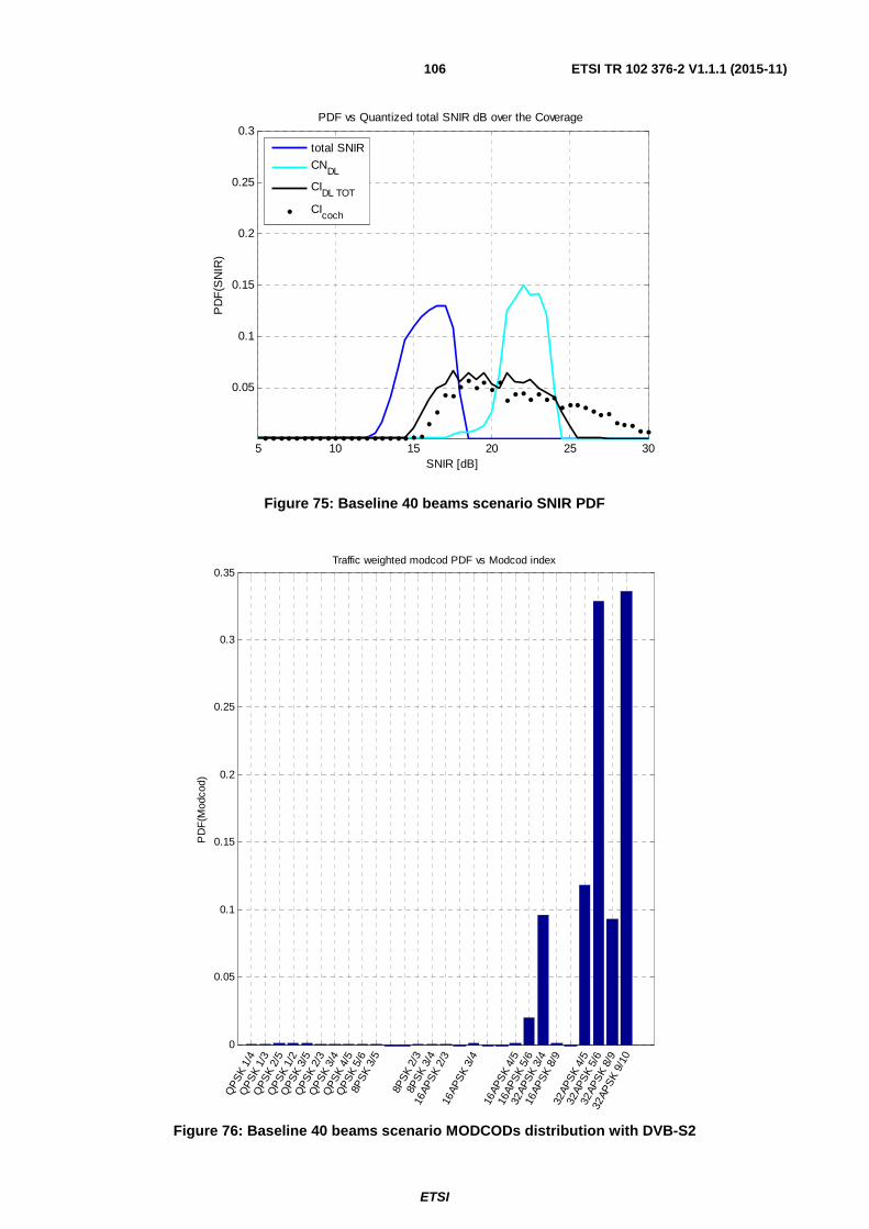
ETSI

ETSI TR 102 376-2 V1.1.1 (2015-11)106

Figure 75: Baseline 40 beams scenario SNIR PDF

Figure 76: Baseline 40 beams scenario MODCODs distribution with DVB-S2

5 10 15 20 25 30

0.05

0.1

0.15

0.2

0.25

0.3PDF vs Quantized total SNIR dB over the Coverage

SNIR [dB]

PD

F(S

NIR

)

total SNIR

CNDL

CIDL TOT

CIcoch

0

0.05

0.1

0.15

0.2

0.25

0.3

0.35Traffic weighted modcod PDF vs Modcod index

PD

F(M

odco

d)

QP

SK

1/4

QP

SK

1/3

QP

SK

2/5

QP

SK

1/2

QP

SK

3/5

QP

SK

2/3

QP

SK

3/4

QP

SK

4/5

QP

SK

5/6

8PS

K 3/

5 8P

SK

2/3

8PS

K 3/

416

APS

K 2/

3 16

APS

K 3/

4 16

APS

K 4/

516

APS

K 5/

632

APS

K 3/

416

APS

K 8/

9 32

APS

K 4/

532

APS

K 5/

632

APS

K 8/

932

APS

K 9/

10

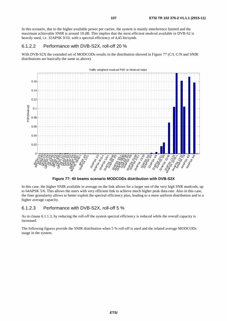
ETSI

ETSI TR 102 376-2 V1.1.1 (2015-11)107

In this scenario, due to the higher available power per carrier, the system is mainly interference limited and the maximum achievable SNIR is around 18 dB. This implies that the most efficient modcod available in DVB-S2 is heavily used, i.e. 32APSK 9/10, with a spectral efficiency of 4,45 bit/symb.

6.1.2.2 Performance with DVB-S2X, roll-off 20 %

With DVB-S2X the extended set of MODCODs results in the distribution showed in Figure 77 (C/I, C/N and SNIR distributions are basically the same as above).

Figure 77: 40 beams scenario MODCODs distribution with DVB-S2X

In this case, the higher SNIR available in average on the link allows for a larger use of the very high SNR modcods, up to 64APSK 5/6. This allows the users with very efficient link to achieve much higher peak data-rate. Also in this case, the finer granularity allows to better exploit the spectral efficiency plan, leading to a more uniform distribution and to a higher average capacity.

6.1.2.3 Performance with DVB-S2X, roll-off 5 %

As in clause 6.1.1.3, by reducing the roll-off the system spectral efficiency is reduced while the overall capacity is increased.

The following figures provide the SNIR distribution when 5 % roll-off is used and the related average MODCODs usage in the system.

0

0.02

0.04

0.06

0.08

0.1

0.12

0.14

0.16

Traffic weighted modcod PDF vs Modcod index

PD

F(M

odco

d)

BPS

K1/

5B

PSK

11/4

5B

PSK

1/3

QP

SK

2/9

QP

SK

1/4

QP

SK

13/4

5Q

PS

K 1/

3Q

PS

K 2/

5Q

PS

K 9/

20Q

PS

K 1/

2

QP

SK

11/2

0Q

PS

K 3/

5Q

PS

K 2/

3Q

PS

K 3/

4Q

PS

K 4/

5

8AP

SK 5

/9-L

8AP

SK 2

6/45

-L 8P

SK

3/5

16AP

SK

1/2-

L

16AP

SK

2/3

16AP

SK

8/15

-L

16AP

SK

5/9-

L

16AP

SK

26/4

5

16AP

SK

3/5

16AP

SK

3/5-

L

16AP

SK

28/4

5

16AP

SK

23/3

6

16AP

SK

3/4

16AP

SK

4/5

16AP

SK

25/3

6

16AP

SK

2/3-

L

16AP

SK

13/1

8

16AP

SK

5/6

32AP

SK

3/4

32AP

SK

4/5

32AP

SK

2/3-

L

32AP

SK

5/6

32AP

SK

32/4

5

32AP

SK

11/1

5

64AP

SK

32/4

5-L

64AP

SK

11/1

5

64AP

SK

7/9

64AP

SK

4/5

64AP

SK

5/6

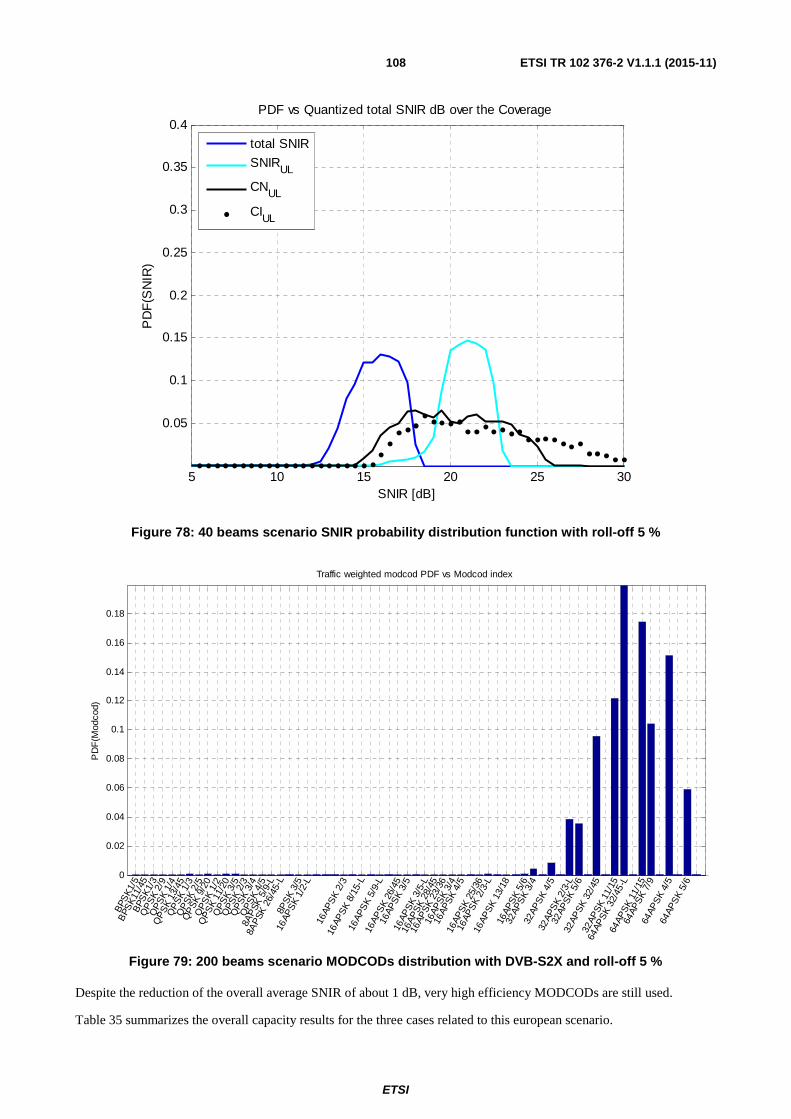
ETSI

ETSI TR 102 376-2 V1.1.1 (2015-11)108

Figure 78: 40 beams scenario SNIR probability distribution function with roll-off 5 %

Figure 79: 200 beams scenario MODCODs distribution with DVB-S2X and roll-off 5 %

Despite the reduction of the overall average SNIR of about 1 dB, very high efficiency MODCODs are still used.

Table 35 summarizes the overall capacity results for the three cases related to this european scenario.

5 10 15 20 25 30

0.05

0.1

0.15

0.2

0.25

0.3

0.35

0.4PDF vs Quantized total SNIR dB over the Coverage

SNIR [dB]

PD

F(S

NIR

)

total SNIR

SNIRUL

CNUL

CIUL

0

0.02

0.04

0.06

0.08

0.1

0.12

0.14

0.16

0.18

Traffic weighted modcod PDF vs Modcod index

PD

F(M

odco

d)

BPS

K1/

5B

PSK

11/4

5B

PSK

1/3

QP

SK

2/9

QP

SK

1/4

QP

SK

13/4

5Q

PS

K 1/

3Q

PS

K 2/

5Q

PS

K 9/

20Q

PS

K 1/

2

QP

SK

11/2

0Q

PS

K 3/

5Q

PS

K 2/

3Q

PS

K 3/

4Q

PS

K 4/

5

8AP

SK 5

/9-L

8AP

SK 2

6/45

-L 8P

SK

3/5

16AP

SK

1/2-

L

16AP

SK

2/3

16AP

SK

8/15

-L

16AP

SK

5/9-

L

16AP

SK

26/4

5

16AP

SK

3/5

16AP

SK

3/5-

L

16AP

SK

28/4

5

16AP

SK

23/3

6

16AP

SK

3/4

16AP

SK

4/5

16AP

SK

25/3

6

16AP

SK

2/3-

L

16AP

SK

13/1

8

16AP

SK

5/6

32AP

SK

3/4

32AP

SK

4/5

32AP

SK

2/3-

L

32AP

SK

5/6

32AP

SK

32/4

5

32AP

SK

11/1

5

64AP

SK

32/4

5-L

64AP

SK

11/1

5

64AP

SK

7/9

64AP

SK

4/5

64AP

SK

5/6

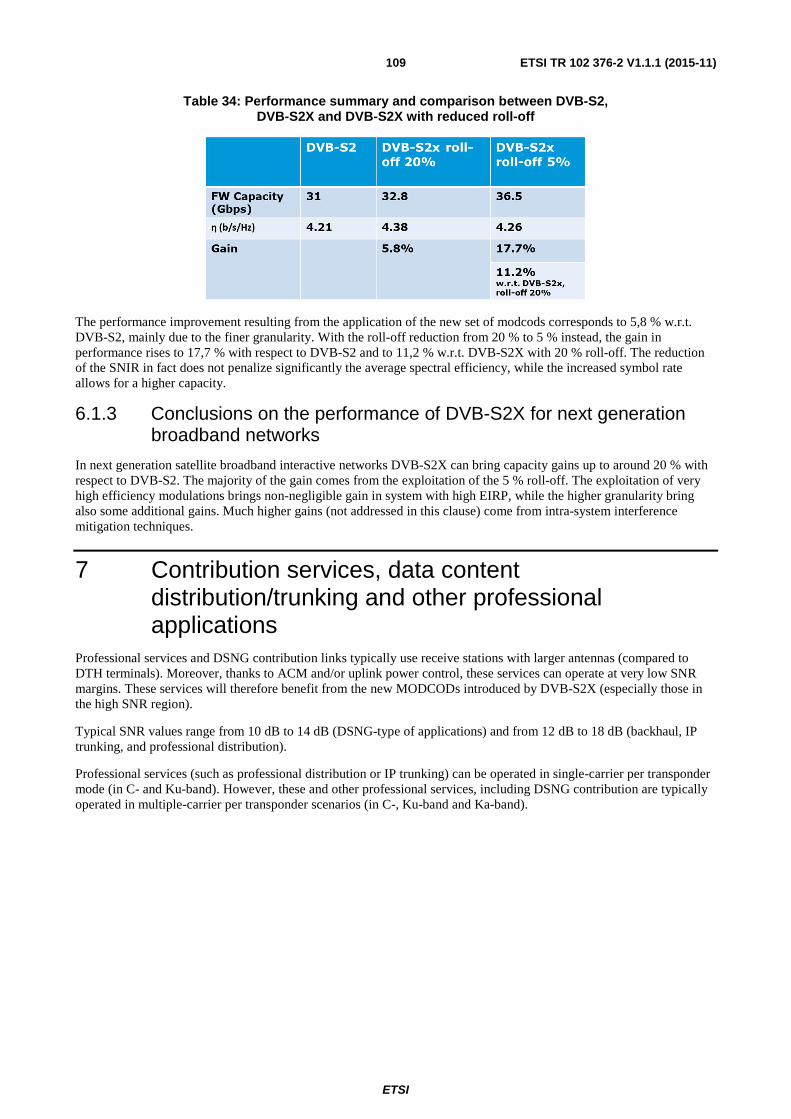
ETSI

ETSI TR 102 376-2 V1.1.1 (2015-11)109

Table 34: Performance summary and comparison between DVB-S2, DVB-S2X and DVB-S2X with reduced roll-off

The performance improvement resulting from the application of the new set of modcods corresponds to 5,8 % w.r.t. DVB-S2, mainly due to the finer granularity. With the roll-off reduction from 20 % to 5 % instead, the gain in performance rises to 17,7 % with respect to DVB-S2 and to 11,2 % w.r.t. DVB-S2X with 20 % roll-off. The reduction of the SNIR in fact does not penalize significantly the average spectral efficiency, while the increased symbol rate allows for a higher capacity.

6.1.3 Conclusions on the performance of DVB-S2X for next generation broadband networks

In next generation satellite broadband interactive networks DVB-S2X can bring capacity gains up to around 20 % with respect to DVB-S2. The majority of the gain comes from the exploitation of the 5 % roll-off. The exploitation of very high efficiency modulations brings non-negligible gain in system with high EIRP, while the higher granularity bring also some additional gains. Much higher gains (not addressed in this clause) come from intra-system interference mitigation techniques.

7 Contribution services, data content distribution/trunking and other professional applications

Professional services and DSNG contribution links typically use receive stations with larger antennas (compared to DTH terminals). Moreover, thanks to ACM and/or uplink power control, these services can operate at very low SNR margins. These services will therefore benefit from the new MODCODs introduced by DVB-S2X (especially those in the high SNR region).

Typical SNR values range from 10 dB to 14 dB (DSNG-type of applications) and from 12 dB to 18 dB (backhaul, IP trunking, and professional distribution).

Professional services (such as professional distribution or IP trunking) can be operated in single-carrier per transponder mode (in C- and Ku-band). However, these and other professional services, including DSNG contribution are typically operated in multiple-carrier per transponder scenarios (in C-, Ku-band and Ka-band).

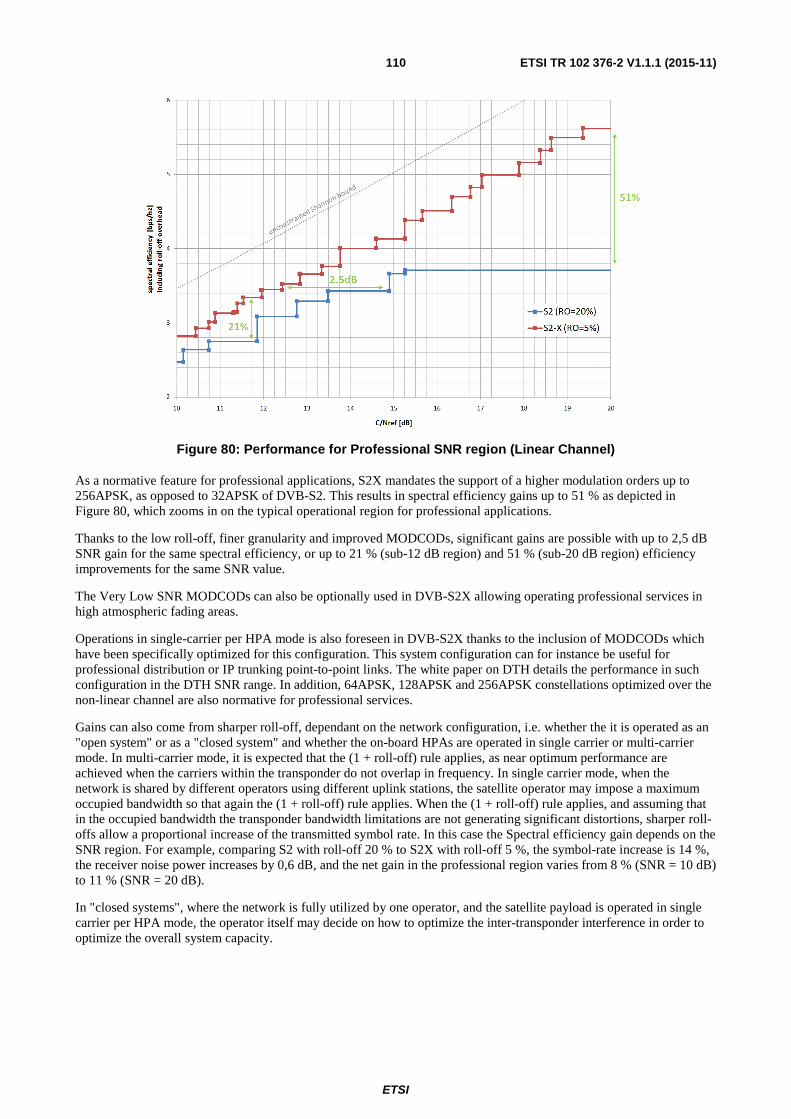
ETSI

ETSI TR 102 376-2 V1.1.1 (2015-11)110

Figure 80: Performance for Professional SNR region (Linear Channel)

As a normative feature for professional applications, S2X mandates the support of a higher modulation orders up to 256APSK, as opposed to 32APSK of DVB-S2. This results in spectral efficiency gains up to 51 % as depicted in Figure 80, which zooms in on the typical operational region for professional applications.

Thanks to the low roll-off, finer granularity and improved MODCODs, significant gains are possible with up to 2,5 dB SNR gain for the same spectral efficiency, or up to 21 % (sub-12 dB region) and 51 % (sub-20 dB region) efficiency improvements for the same SNR value.

The Very Low SNR MODCODs can also be optionally used in DVB-S2X allowing operating professional services in high atmospheric fading areas.

Operations in single-carrier per HPA mode is also foreseen in DVB-S2X thanks to the inclusion of MODCODs which have been specifically optimized for this configuration. This system configuration can for instance be useful for professional distribution or IP trunking point-to-point links. The white paper on DTH details the performance in such configuration in the DTH SNR range. In addition, 64APSK, 128APSK and 256APSK constellations optimized over the non-linear channel are also normative for professional services.

Gains can also come from sharper roll-off, dependant on the network configuration, i.e. whether the it is operated as an "open system" or as a "closed system" and whether the on-board HPAs are operated in single carrier or multi-carrier mode. In multi-carrier mode, it is expected that the (1 + roll-off) rule applies, as near optimum performance are achieved when the carriers within the transponder do not overlap in frequency. In single carrier mode, when the network is shared by different operators using different uplink stations, the satellite operator may impose a maximum occupied bandwidth so that again the (1 + roll-off) rule applies. When the (1 + roll-off) rule applies, and assuming that in the occupied bandwidth the transponder bandwidth limitations are not generating significant distortions, sharper roll-offs allow a proportional increase of the transmitted symbol rate. In this case the Spectral efficiency gain depends on the SNR region. For example, comparing S2 with roll-off 20 % to S2X with roll-off 5 %, the symbol-rate increase is 14 %, the receiver noise power increases by 0,6 dB, and the net gain in the professional region varies from 8 % (SNR = 10 dB) to 11 % (SNR = 20 dB).

In "closed systems", where the network is fully utilized by one operator, and the satellite payload is operated in single carrier per HPA mode, the operator itself may decide on how to optimize the inter-transponder interference in order to optimize the overall system capacity.

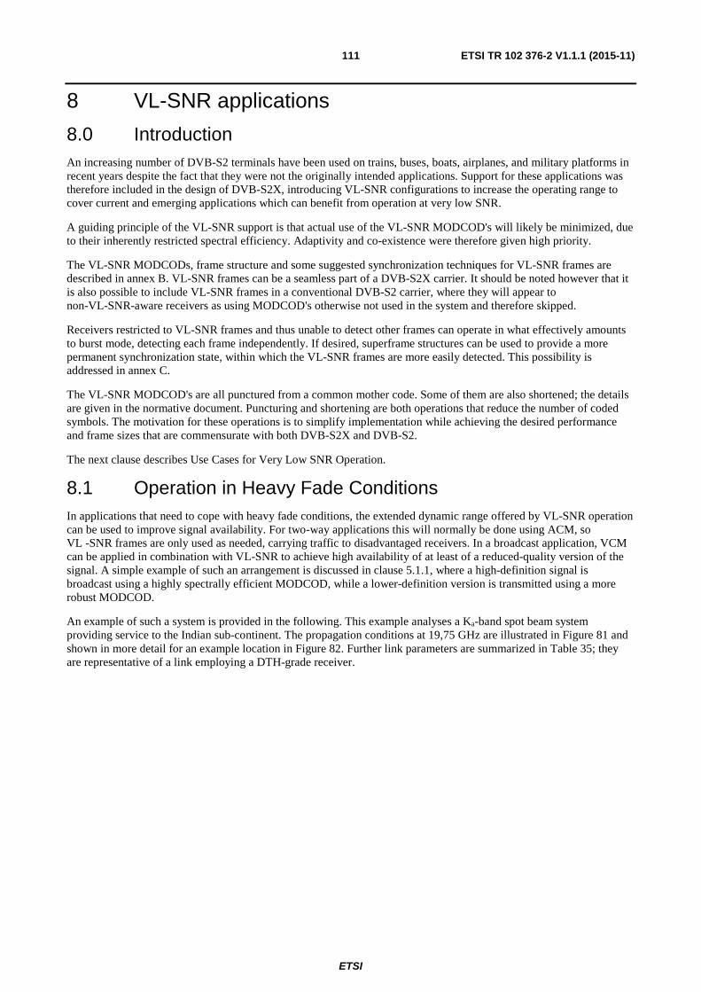
ETSI

ETSI TR 102 376-2 V1.1.1 (2015-11)111

8 VL-SNR applications

8.0 Introduction An increasing number of DVB-S2 terminals have been used on trains, buses, boats, airplanes, and military platforms in recent years despite the fact that they were not the originally intended applications. Support for these applications was therefore included in the design of DVB-S2X, introducing VL-SNR configurations to increase the operating range to cover current and emerging applications which can benefit from operation at very low SNR.

A guiding principle of the VL-SNR support is that actual use of the VL-SNR MODCOD's will likely be minimized, due to their inherently restricted spectral efficiency. Adaptivity and co-existence were therefore given high priority.

The VL-SNR MODCODs, frame structure and some suggested synchronization techniques for VL-SNR frames are described in annex B. VL-SNR frames can be a seamless part of a DVB-S2X carrier. It should be noted however that it is also possible to include VL-SNR frames in a conventional DVB-S2 carrier, where they will appear to non-VL-SNR-aware receivers as using MODCOD's otherwise not used in the system and therefore skipped.

Receivers restricted to VL-SNR frames and thus unable to detect other frames can operate in what effectively amounts to burst mode, detecting each frame independently. If desired, superframe structures can be used to provide a more permanent synchronization state, within which the VL-SNR frames are more easily detected. This possibility is addressed in annex C.

The VL-SNR MODCOD's are all punctured from a common mother code. Some of them are also shortened; the details are given in the normative document. Puncturing and shortening are both operations that reduce the number of coded symbols. The motivation for these operations is to simplify implementation while achieving the desired performance and frame sizes that are commensurate with both DVB-S2X and DVB-S2.

The next clause describes Use Cases for Very Low SNR Operation.

8.1 Operation in Heavy Fade Conditions In applications that need to cope with heavy fade conditions, the extended dynamic range offered by VL-SNR operation can be used to improve signal availability. For two-way applications this will normally be done using ACM, so VL -SNR frames are only used as needed, carrying traffic to disadvantaged receivers. In a broadcast application, VCM can be applied in combination with VL-SNR to achieve high availability of at least of a reduced-quality version of the signal. A simple example of such an arrangement is discussed in clause 5.1.1, where a high-definition signal is broadcast using a highly spectrally efficient MODCOD, while a lower-definition version is transmitted using a more robust MODCOD.

An example of such a system is provided in the following. This example analyses a Ka-band spot beam system providing service to the Indian sub-continent. The propagation conditions at 19,75 GHz are illustrated in Figure 81 and shown in more detail for an example location in Figure 82. Further link parameters are summarized in Table 35; they are representative of a link employing a DTH-grade receiver.

ETSI

ETSI TR 102 376-2 V1.1.1 (2015-11)112

Figure 81: Ka-band propagation in area illuminated from 60° E

Figure 82: Cumulative rain fade statistics for example location

Table 35: Link parameters for VL-SNR example

10-1

100

101

102

0

2

4

6

8

10

12

14

16

Percentage of time attenuation exceeded

Att

enua

tion,

dB

19.75 GHz circular, 6.3N 80.6E, Sat 60E

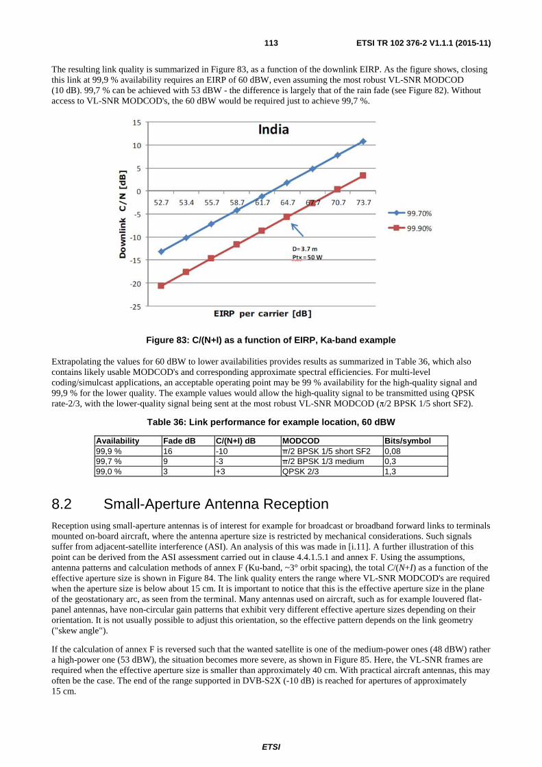
ETSI

ETSI TR 102 376-2 V1.1.1 (2015-11)113

The resulting link quality is summarized in Figure 83, as a function of the downlink EIRP. As the figure shows, closing this link at 99,9 % availability requires an EIRP of 60 dBW, even assuming the most robust VL-SNR MODCOD (10 dB). 99,7 % can be achieved with 53 dBW - the difference is largely that of the rain fade (see Figure 82). Without access to VL-SNR MODCOD's, the 60 dBW would be required just to achieve 99,7 %.

Figure 83: C/(N+I) as a function of EIRP, Ka-band example

Extrapolating the values for 60 dBW to lower availabilities provides results as summarized in Table 36, which also contains likely usable MODCOD's and corresponding approximate spectral efficiencies. For multi-level coding/simulcast applications, an acceptable operating point may be 99 % availability for the high-quality signal and 99,9 % for the lower quality. The example values would allow the high-quality signal to be transmitted using QPSK rate-2/3, with the lower-quality signal being sent at the most robust VL-SNR MODCOD (π/2 BPSK 1/5 short SF2).

Table 36: Link performance for example location, 60 dBW

Availability Fade dB C/(N+I) dB MODCOD Bits/symbol 99,9 % 16 -10 π/2 BPSK 1/5 short SF2 0,08 99,7 % 9 -3 π/2 BPSK 1/3 medium 0,3 99,0 % 3 +3 QPSK 2/3 1,3

8.2 Small-Aperture Antenna Reception Reception using small-aperture antennas is of interest for example for broadcast or broadband forward links to terminals mounted on-board aircraft, where the antenna aperture size is restricted by mechanical considerations. Such signals suffer from adjacent-satellite interference (ASI). An analysis of this was made in [i.11]. A further illustration of this point can be derived from the ASI assessment carried out in clause 4.4.1.5.1 and annex F. Using the assumptions, antenna patterns and calculation methods of annex F (Ku-band, ~3° orbit spacing), the total C/(N+I) as a function of the effective aperture size is shown in Figure 84. The link quality enters the range where VL-SNR MODCOD's are required when the aperture size is below about 15 cm. It is important to notice that this is the effective aperture size in the plane of the geostationary arc, as seen from the terminal. Many antennas used on aircraft, such as for example louvered flat-panel antennas, have non-circular gain patterns that exhibit very different effective aperture sizes depending on their orientation. It is not usually possible to adjust this orientation, so the effective pattern depends on the link geometry ("skew angle").

If the calculation of annex F is reversed such that the wanted satellite is one of the medium-power ones (48 dBW) rather a high-power one (53 dBW), the situation becomes more severe, as shown in Figure 85. Here, the VL-SNR frames are required when the effective aperture size is smaller than approximately 40 cm. With practical aircraft antennas, this may often be the case. The end of the range supported in DVB-S2X (-10 dB) is reached for apertures of approximately 15 cm.

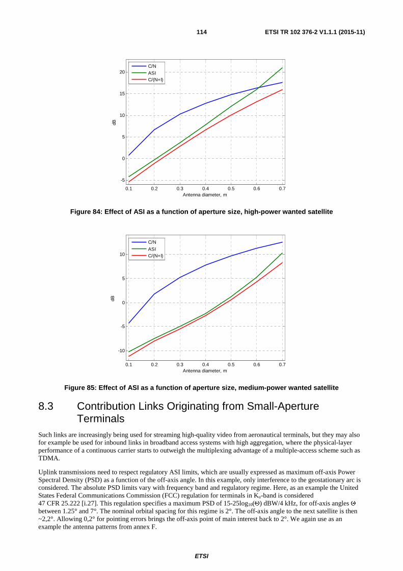
ETSI

ETSI TR 102 376-2 V1.1.1 (2015-11)114

Figure 84: Effect of ASI as a function of aperture size, high-power wanted satellite

Figure 85: Effect of ASI as a function of aperture size, medium-power wanted satellite

8.3 Contribution Links Originating from Small-Aperture Terminals

Such links are increasingly being used for streaming high-quality video from aeronautical terminals, but they may also for example be used for inbound links in broadband access systems with high aggregation, where the physical-layer performance of a continuous carrier starts to outweigh the multiplexing advantage of a multiple-access scheme such as TDMA.

Uplink transmissions need to respect regulatory ASI limits, which are usually expressed as maximum off-axis Power Spectral Density (PSD) as a function of the off-axis angle. In this example, only interference to the geostationary arc is considered. The absolute PSD limits vary with frequency band and regulatory regime. Here, as an example the United States Federal Communications Commission (FCC) regulation for terminals in Ku-band is considered 47 CFR 25.222 [i.27]. This regulation specifies a maximum PSD of 15-25log10(Θ) dBW/4 kHz, for off-axis angles Θ between 1.25° and 7°. The nominal orbital spacing for this regime is 2°. The off-axis angle to the next satellite is then ~2,2°. Allowing 0,2° for pointing errors brings the off-axis point of main interest back to 2°. We again use as an example the antenna patterns from annex F.

0.1 0.2 0.3 0.4 0.5 0.6 0.7

-5

0

5

10

15

20

Antenna diameter, m

dB

C/N

ASIC/(N+I)

0.1 0.2 0.3 0.4 0.5 0.6 0.7

-10

-5

0

5

10

Antenna diameter, m

dB

C/N

ASIC/(N+I)

ETSI

ETSI TR 102 376-2 V1.1.1 (2015-11)115

At the 2° offset, the intercept points between the mask and the antenna patterns all occur in the main lobe, so the effect of the regulatory limits can be determined simply by considering the gain difference between the boresight and the offset angle. This is illustrated in Figure 86, as a function of antenna size.

Given the maximum PSD at the offset angle (Po), the maximum boresight PSD is higher by the gain difference ΔG shown in Figure 86. Further given the path loss Lp, the satellite receive G/T and the reference bandwidth Br, we can compute the maximum achievable C/N as:

)(log10 10 rBpo Bk

T

GLGP

N

C −−+−Δ+=

where kB = -228,6 dB (J/K) is Boltzmann's constant. The maximum PSD at 2° offset is -2,3 dBW/4 kHz; hence Br = 4000. Further, a path loss Lp of 208 dB and a satellite receive G/T of 6 dB is assumed, corresponding to a typical regional Ku-band system. The resulting maximum achievable C/N is shown in Figure 87. This figure does not take into account any interference or atmospheric impairments. We see that VL-SNR MODCOD's allow operation with antenna sizes down to approximately 35 cm. As for the downlink operation (see clause 8.2), it is noted that this is the effective aperture size, which can vary substantially with the orientation of the antenna relative to the geostationary orbit.

Figure 86: Example gain differences between boresight and pointing to next satellite, dB

Figure 87: Maximum achievable C/N for example system, dB

10 20 30 40 50 60 70 800

1

2

3

4

5

6

7

8

9

10

Antenna diameter, cm

Diff

eren

ce b

etw

een

gain

at

bore

sigh

t an

d 2°

off

set,

dB

10 20 30 40 50 60 70 80-12

-11

-10

-9

-8

-7

-6

-5

-4

-3

-2

Antenna diameter, cm

Max

imum

ach

ieva

ble

C/N

, dB

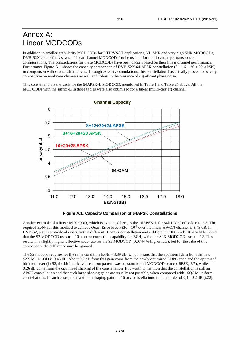
ETSI

ETSI TR 102 376-2 V1.1.1 (2015-11)116

Annex A: Linear MODCODs In addition to smaller granularity MODCODs for DTH/VSAT applications, VL-SNR and very high SNR MODCODs, DVB-S2X also defines several "linear channel MODCODs" to be used in for multi-carrier per transponder configurations. The constellations for these MODCODs have been chosen based on their linear channel performance. For instance Figure A.1 shows the capacity comparison of DVB-S2X 64-APSK constellation (8 + 16 + 20 + 20 APSK) in comparison with several alternatives. Through extensive simulations, this constellation has actually proven to be very competitive on nonlinear channels as well and robust in the presence of significant phase noise.

This constellation is the basis for the 64APSK-L MODCOD, mentioned in Table 1 and Table 25 above. All the MODCODs with the suffix -L in those tables were also optimized for a linear (multi-carrier) channel.

Figure A.1: Capacity Comparison of 64APSK Constellations

Another example of a linear MODCOD, which is explained here, is the 16APSK-L for 64k LDPC of code rate 2/3. The required Es/N0 for this modcod to achieve Quasi Error Free FER = 10-5 over the linear AWGN channel is 8,43 dB. In DVB-S2, a similar modcod exists, with a different 16APSK constellation and a different LDPC code. It should be noted that the S2 MODCOD uses tr = 10 as error correction capability for BCH, while the S2X MODCOD uses t = 12. This results in a slightly higher effective code rate for the S2 MODCOD (0,0744 % higher rate), but for the sake of this comparison, the difference may be ignored.

The S2 modcod requires for the same condition Es/N0 = 8,89 dB, which means that the additional gain from the new S2X MODCOD is 0,46 dB. About 0,2 dB from this gain come from the newly optimized LDPC code and the optimized bit interleaver (in S2, the bit interleaver read-out pattern was constant for all MODCODs except 8PSK, 3/5), while 0,26 dB come from the optimized shaping of the constellation. It is worth to mention that the constellation is still an APSK constellation and that such large shaping gains are usually not possible, when compared with 16QAM uniform constellations. In such cases, the maximum shaping gain for 16-ary constellations is in the order of 0,1 - 0,2 dB [i.22].

ETSI

ETSI TR 102 376-2 V1.1.1 (2015-11)117

Annex B: DVB-S2X VL-SNR Modes

B.1 VL-SNR MODCODs DVB-S2X has addressed the demand for MODCODs operating in critical SNR scenarios by defining low rate, π/2 BPSK MODCODs that can operate at Es/No as low as -10 dB. π/2 BPSK modulation has been preferred over BPSK due to its better spectral properties. Furthermore, as described in Appendix B, DVB-S2X allows the insertion of VL-SNR frames into regular DVB-S2X or legacy DVB-S2 frames without causing extra synchronization overhead to those frames.

The nine VL-SNR MODCODs are given in Table 38. As shown in the table, all of the MODCODs are punctured from a mother code. Some of the MODCODs are also shortened. Both puncturing and shortening are operations that reduce the number of coded symbols. The motivation for these operations is to make the size of VL-SNR frames, in the presence of 900 symbol mobile header and extra pilot symbols, the same as the size of a legacy DVB-S2 frame size. That way, the new VL-SNR frames can be used together with legacy S2 VCM/ACM receivers where the legacy receivers would just skip the VL-SNR frames.

For some MODCODs, spreading by a factor of 2 (SF2) is applicable. This spreading refers to bit-wise repetition of the encoded bits. If the encoded bit sequence is b0, b1, b2, etc., the repetition will transform this into b0, b0, b1, b1, b2, b2, etc., which is then fed to the π/2 BPSK bit-to-symbol mapper.

Table B.1: VL-SNR MODCODs

MODCOD Xs P Xp QPSK 2/9 normal 0 15 3240

π/2 BPSK 1/5 medium 640 25 980 π/2 BPSK 11/45 medium 0 15 1620 π/2 BPSK 1/3 medium 0 13 1620 π/2 BPSK 1/5 short SF2 560 30 250 π/2 BPSK 11/45 short SF2 0 15 810

π/2 BPSK 1/5 short 0 10 1224 π/2 BPSK 4/15 short 0 8 1224 π/2 BPSK 1/3 short 0 8 1224

The exact algorithm for puncturing/shortening is given in the standard. The performance of the VL-SNR MODCODs is shown in Figure B.1.

ETSI

ETSI TR 102 376-2 V1.1.1 (2015-11)118

ETSI

ETSI TR 102 376-2 V1.1.1 (2015-11)119

ETSI

ETSI TR 102 376-2 V1.1.1 (2015-11)120

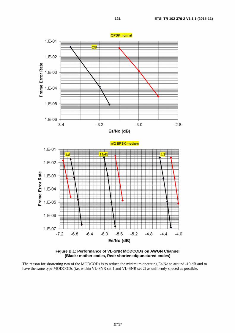
ETSI

ETSI TR 102 376-2 V1.1.1 (2015-11)121

Figure B.1: Performance of VL-SNR MODCODs on AWGN Channel (Black: mother codes, Red: shortened/punctured codes)

The reason for shortening two of the MODCODs is to reduce the minimum operating Es/No to around -10 dB and to have the same type MODCODs (i.e. within VL-SNR set 1 and VL-SNR set 2) as uniformly spaced as possible.

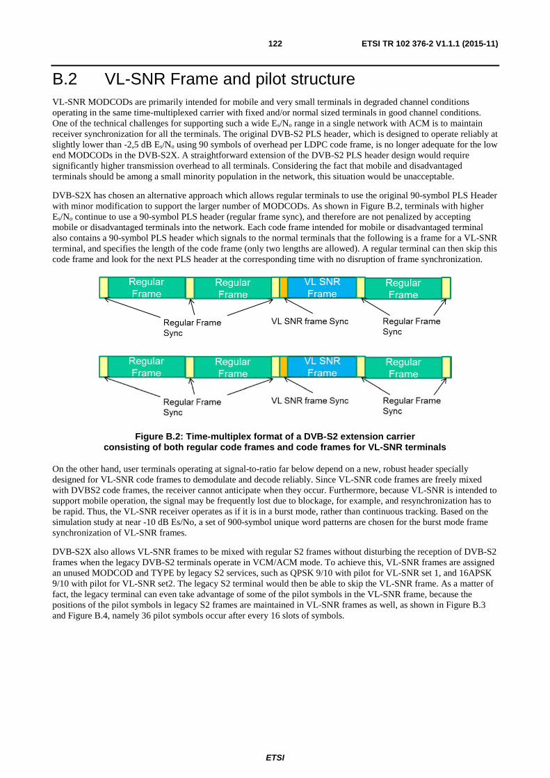
ETSI

ETSI TR 102 376-2 V1.1.1 (2015-11)122

B.2 VL-SNR Frame and pilot structure VL-SNR MODCODs are primarily intended for mobile and very small terminals in degraded channel conditions operating in the same time-multiplexed carrier with fixed and/or normal sized terminals in good channel conditions. One of the technical challenges for supporting such a wide Es/No range in a single network with ACM is to maintain receiver synchronization for all the terminals. The original DVB-S2 PLS header, which is designed to operate reliably at slightly lower than -2,5 dB Es/No using 90 symbols of overhead per LDPC code frame, is no longer adequate for the low end MODCODs in the DVB-S2X. A straightforward extension of the DVB-S2 PLS header design would require significantly higher transmission overhead to all terminals. Considering the fact that mobile and disadvantaged terminals should be among a small minority population in the network, this situation would be unacceptable.

DVB-S2X has chosen an alternative approach which allows regular terminals to use the original 90-symbol PLS Header with minor modification to support the larger number of MODCODs. As shown in Figure B.2, terminals with higher Es/No continue to use a 90-symbol PLS header (regular frame sync), and therefore are not penalized by accepting mobile or disadvantaged terminals into the network. Each code frame intended for mobile or disadvantaged terminal also contains a 90-symbol PLS header which signals to the normal terminals that the following is a frame for a VL-SNR terminal, and specifies the length of the code frame (only two lengths are allowed). A regular terminal can then skip this code frame and look for the next PLS header at the corresponding time with no disruption of frame synchronization.

Figure B.2: Time-multiplex format of a DVB-S2 extension carrier consisting of both regular code frames and code frames for VL-SNR terminals

On the other hand, user terminals operating at signal-to-ratio far below depend on a new, robust header specially designed for VL-SNR code frames to demodulate and decode reliably. Since VL-SNR code frames are freely mixed with DVBS2 code frames, the receiver cannot anticipate when they occur. Furthermore, because VL-SNR is intended to support mobile operation, the signal may be frequently lost due to blockage, for example, and resynchronization has to be rapid. Thus, the VL-SNR receiver operates as if it is in a burst mode, rather than continuous tracking. Based on the simulation study at near -10 dB Es/No, a set of 900-symbol unique word patterns are chosen for the burst mode frame synchronization of VL-SNR frames.

DVB-S2X also allows VL-SNR frames to be mixed with regular S2 frames without disturbing the reception of DVB-S2 frames when the legacy DVB-S2 terminals operate in VCM/ACM mode. To achieve this, VL-SNR frames are assigned an unused MODCOD and TYPE by legacy S2 services, such as QPSK 9/10 with pilot for VL-SNR set 1, and 16APSK 9/10 with pilot for VL-SNR set2. The legacy S2 terminal would then be able to skip the VL-SNR frame. As a matter of fact, the legacy terminal can even take advantage of some of the pilot symbols in the VL-SNR frame, because the positions of the pilot symbols in legacy S2 frames are maintained in VL-SNR frames as well, as shown in Figure B.3 and Figure B.4, namely 36 pilot symbols occur after every 16 slots of symbols.

ETSI

ETSI TR 102 376-2 V1.1.1 (2015-11)123

Figure B.3: VL-SNR Set1 Frame Structure

Figure B.4: VL-SNR Set2 Frame Structure

In specific cases VL-SNR frames according to S2X standard may be inserted in a DVB-S2 transmission without disturbing the regular reception of the DVB-S2 frames by legacy receivers capable of ACM/VCM operation. In order for legacy receivers to continue exploit pilot symbols inserted in VL-SNR frames, these pilots symbols should be scrambled in the same way as DVB-S2. On the other hand, VL-SNR header symbols should not be scrambled since they are used in the synchronization of VL-SNR frames. As a result of these two requirements, scrambling sequence is reset at the beginning of VL-SNR header. The scrambling sequence is then advanced during the VL-SNR header, but it is not applied until the FEC frame starts.

B.3 VL-SNR MODCOD Signalling Excluding the two dummy symbols at the beginning and the end, each of the 900-symbol unique words consists of 16 symbol sections of 56 symbols each. Each of the segments can be transmitted as is or in reversed polarity. The polarity of these segments signals the MODCOD of the following code frame, as summarized in Table B.2. These patterns are taken from Walsh-Hadamard sequence of length 16 and are therefore mutually orthogonal to one another.

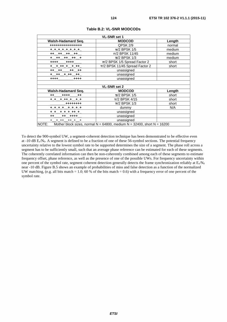
ETSI

ETSI TR 102 376-2 V1.1.1 (2015-11)124

Table B.2: VL-SNR MODCODs

VL-SNR set 1 Walsh-Hadamard Seq. MODCOD Length

++++++++++++++++ QPSK 2/9 normal +_+_+_+_+_+_+_+_ π/2 BPSK 1/5 medium ++__++__++__++__ π/2 BPSK 11/45 medium +__++__++__++__+ π/2 BPSK 1/3 medium ++++____++++____ π/2 BPSK 1/5 Spread Factor 2 short +__+_++_+__+_++_ π/2 BPSK 11/45 Spread Factor 2 short ++__++____++__++ unassigned +__++__+_++__++_ unassigned ++++________++++ unassigned

VL-SNR set 2

Walsh-Hadamard Seq. MODCOD Length ++____++++____++ π/2 BPSK 1/5 short +_+__+_++_+__+_+ π/2 BPSK 4/15 short ________++++++++ π/2 BPSK 1/3 short +_+_+_+__+_+_+_+ dummy N/A +_+__+_+_+_++_+_ unassigned ++____++__++++__ unassigned +__+_++__++_+__+ unassigned

NOTE: Mother block sizes, normal N = 64800, medium N = 32400, short N = 16200

To detect the 900-symbol UW, a segment-coherent detection technique has been demonstrated to be effective even at -10 dB Es/N0. A segment is defined to be a fraction of one of these 56-symbol sections. The potential frequency uncertainty relative to the lowest symbol rate to be supported determines the size of a segment. The phase roll across a segment has to be sufficiently small, such that an average phase reference can be estimated for each of these segments. The coherently correlated information can then be non-coherently combined among each of these segments to estimate frequency offset, phase reference, as well as the presence of one of the possible UWs. For frequency uncertainty within one percent of the symbol rate, segment coherent detection generally detects the frame synchronization reliably at Es/N0 near -10 dB. Figure B.5 shows an example of probabilities of miss and false detection as a function of the normalized UW matching, (e.g. all bits match = 1.0; 60 % of the bits match = 0.6) with a frequency error of one percent of the symbol rate.

ETSI

ETSI TR 102 376-2 V1.1.1 (2015-11)125

Figure B.5: Probabilities of miss and false detection vs. normalized UW matching at Es/No = -9,6 dB with frequency offset at one percent symbol rate,

symbol timing uncertainty uniformly distributed between -½ and ½ symbol intervals and phase noise (Ka 2012)

For cases where frequency uncertainty is greater than one percent of the symbol rate, a quadri-correlator frequency acquisition loop [i.23] may be used to reduce the frequency uncertainty down to less than one percent, after which the segment-coherent combining approach can be applied. Figure B.6 shows that the quadri-correlator acquires the frequency from a large frequency offset near 3 percent of the symbol rate at -9,6 dB Es/N0 after several hundred thousand symbols of root-Nyquist filtered APSK modulated symbols as expected.

ETSI

ETSI TR 102 376-2 V1.1.1 (2015-11)126

Figure B.6: Frequency acquisition performance of a quadri-correlator loop at Es/No of -9,6 dB

B.4 VL-SNR Dummy Frames Even though the quadri-correlator frequency acquisition loop performs well in most circumstances, it can falsely lock to an adjacent carrier when the frequency error with respect to the symbol rate is greater than the roll-off factor of the filter, as illustrated by Figure B.7. Here, the frequency error is ΔRs, and the roll-off factor is α. Since the receive filter takes in a non-negligible amount of the energy from an adjacent channel, the quadri-correlator has a small probability to lock to the adjacent channel. Since the receiver has no knowledge when a VL-SNR code frame may be transmitted, it may stay locked to the adjacent channel unless a time-out mechanism is available to force the receiver to break the frequency lock and reacquire its carrier again.

0

0,005

0,01

0,015

0,02

0,025

0,03

0 2 4 6 8

rms

freq

uen

cy e

rro

r (a

ymb

ol R

ate)

No. of Symbols (million)

Residual frequency error

Simulation

predict

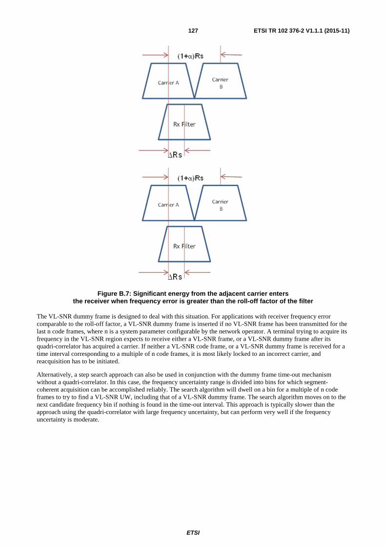
ETSI

ETSI TR 102 376-2 V1.1.1 (2015-11)127

Figure B.7: Significant energy from the adjacent carrier enters the receiver when frequency error is greater than the roll-off factor of the filter

The VL-SNR dummy frame is designed to deal with this situation. For applications with receiver frequency error comparable to the roll-off factor, a VL-SNR dummy frame is inserted if no VL-SNR frame has been transmitted for the last n code frames, where n is a system parameter configurable by the network operator. A terminal trying to acquire its frequency in the VL-SNR region expects to receive either a VL-SNR frame, or a VL-SNR dummy frame after its quadri-correlator has acquired a carrier. If neither a VL-SNR code frame, or a VL-SNR dummy frame is received for a time interval corresponding to a multiple of n code frames, it is most likely locked to an incorrect carrier, and reacquisition has to be initiated.

Alternatively, a step search approach can also be used in conjunction with the dummy frame time-out mechanism without a quadri-correlator. In this case, the frequency uncertainty range is divided into bins for which segment-coherent acquisition can be accomplished reliably. The search algorithm will dwell on a bin for a multiple of n code frames to try to find a VL-SNR UW, including that of a VL-SNR dummy frame. The search algorithm moves on to the next candidate frequency bin if nothing is found in the time-out interval. This approach is typically slower than the approach using the quadri-correlator with large frequency uncertainty, but can perform very well if the frequency uncertainty is moderate.

ETSI

ETSI TR 102 376-2 V1.1.1 (2015-11)128

Annex C: Super-Framing structure

C.0 General description The super-framing structure is added to the DVB-S2X specification ETSI EN 302 307-2 [i.2] in annex E as an optional transmission mode and is designed such to combine the benefits of the conventional transmission of PLFRAMEs (e.g. just-in-time transmission of PLFRAMEs, which can in general be of different sizes and MODCOD) with the ones of a regular framing structure. This regular structure implies substantial benefits in demodulation performance as well as in enabling new functionalities.

In particular, the super-framing structure:

• Enables new techniques like beam-hopping, precoding see clause C.5, and multi-user detection at the user terminal.

• Is future-proof because of signalling of the super-frame content format on a per super-frame basis, which allows introducing new formats in a clean way (receiver processes only known formats) as well as enables even a format multiplex.

• Achieves a robust receiver synchronization under severe channel conditions (e.g. VL-SNR or mobility):

- Timing synchronization and symbol rate offset estimation.

- Early frequency offset estimation and correction.

- Phase tracking (re-initialization) support.

• Enhances interference resilience and mitigation techniques due to super-frame aligned two-way scrambling (two parallel scramblers independently configurable) and use of orthogonal Walsh-Hadamard (WH) sequences as reference/ training sequences (e.g. for pilots).

All these advantages are supported at the expense of a very limited increase of framing overhead.

The super-framing concept follows the rule of "super-frame as a container" hosting format-specific content as visualized in Figure C.1. The preamble always consists of:

• Start of super-frame (SOSF) as a reference/ training sequence (chosen from a set of Walsh-Hadamard (WH) sequences).

• Super-frame format indicator (SFFI), which signals the actual format of the super-frame content and is protected by a simplex code in combination with spreading.

Since all super-frame transmissions have in common this preamble and a constant super-frame length independent of the content, a receiver can always detect and synchronize to this structure. Thus, prior to any payload processing robust synchronization w.r.t. carrier frequency offset and timing (frequency) offset can be established as demonstrated in clause C.3, where also the structure of the SFFI can be exploited. After decoding the SFFI, the receivers can identify unsupported or unwanted formats and discard these super-frames but stays synchronized.

ETSI

ETSI TR 102 376-2 V1.1.1 (2015-11)129

Figure C.1: Super-frames of constant length - independent of the choice of a super-frame format, which specifies the resource allocation and content

In particular, the super-framing structure is meant to give improvement compared to the conventional framing approach w.r.t. the following issues:

• Simplified and more reliable PLFRAME / PLH detection and tracking due to constant super-frame length and a resource allocation grid compared to the irregular frame lengths or framing structure of the conventional framing approach.

• PLH protection is enhanced by super-frame aligned scrambling (potentially of different n per carrier) compared to a non-programmable physical layer scrambling sequence for the PLH.

• Regular pilot-grid - in some formats even regular over super-frame borders - simplifies the phase tracking task compared to a per PLFRAME processing.

• Selectable and orthogonal pilot sequences to reduce the co-channel or adjacent interference compared to a single sequences in the conventional framing approach.

• VL-SNR synchronization is simplified and more reliable due to the super-frame structure compared to the conventional way of detecting the VL-SNR frames in burst mode (on a per-symbol search grid).

C.1 Application Scenarios and System Setup

C.1.0 Introduction to Super-Frame Formats The super-frame concept provides the ability to be applied in new network topologies required for new techniques like precoding or beam-hopping/switching. Suitable super-frame formats are identified in the following clauses.

C.1.1 Focus of Super-Frame Formats The five different super-frame formats exhibit different features according to their focus:

• Format 0: DVB-S2X including VL-SNR frame.

• Wide re-use of the DVB-S2X specification ETSI EN 302 307-2 [i.2] is made, while only the pilot structure has been modified in comparison to the conventional scheme. Therefore, the application scenarios remain the same as for the conventional scheme (see main clauses of the present document), where the super-framing and the related pilot structure give additional support to the receiver synchronization being of special value under VL-SNR conditions.

• Format 1: Legacy support of DVB-S2.

• Like in format 0, wide re-use of the DVB-S2 specification ETSI EN 302 307-1 [i.1] is made, while only the pilot structure has been modified in comparison to the conventional scheme. The main focus is here on legacy support having the same application scenarios as stated in ETSI TR 102 376-1 [i.3].

• Format 2 and 3: Bundled PLFRAME formats.

ETSI

ETSI TR 102 376-2 V1.1.1 (2015-11)130

• These two formats specify bundling of XFECFRAMEs in order to achieve constant size PLFRAMEs independent of the used MODCOD. This feature is the result of the optimization for precoding to enhance the capabilities of broadband interactive networks as shown in clause C.5, but also DSNG and professional services.

• Format 4: Flexible multi-purpose format.

• This format focus mainly on wide-band transmission since its PLH provides the SID/ISI/TSN according to the application case. Nevertheless, it is also suitable for other application cases as indicated by Table 1 in ETSI EN 302 307-2 [i.2].

• Four different PLH protection levels enables support of scenarios for VL-SNR applications but also high efficiency signalling for the high SNR and high throughput case. Although the protection level can change on a per super-frame basis which is advantageous for traffic shaping, it is always assured that each receiver can perform PLH tracking.

C.1.2 Comparison of Super-Frame Format Features The following comparison table gives an overview over the features and configuration possibilities of the different super-frame (SF) formats.

Table C.1: Comparison of features of the different super-frame formats

Feature Format 0 Format 1 Format 2 Format 3 Format 4 Resource

allocation of PLFRAMEs (see note)

Capacity-Unit-based grid

(CU = SLOT)

Capacity-Unit-based grid

(CU = SLOT)

Static grid aligned to super-frame

and constant size bundled

PLFRAMEs

Static grid aligned to super-frame

and constant size bundled

PLFRAMEs

Capacity-Unit-based grid

(CU = SLOT)

VL-SNR support VL-SNR frame for burst mode reception

No PLS spreading 6 and static location

PLS spreading 4 and static location

Pointer of first PLH and PLS

spreading for VL-SNR PLH tracking

Special pilots for VL-SNR

Yes No No No Yes

Super-frame pilot switching

ON/OFF

Yes Yes No, always ON No, always ON Yes

Super-frame pilot periodicity

Periodicity kept from SF to SF

Periodicity kept from SF to SF

Periodicity SF-internal

Periodicity SF-internal

Periodicity kept from SF to SF

Wide-band support

Yes, when using the extended PLHEADER

No No No Yes, extended PLHEADER always used

Payload data scrambling

PLFRAME scrambling

PLFRAME scrambling

SF-aligned payload data scrambling

SF-aligned payload data scrambling

SF-aligned payload data scrambling

MODCOD-specific Training

data

No No Pilot field P2 respects signalled

MODCOD

Pilot field P2 respects signalled

MODCOD

Dummy frames respect signalled

MODCOD Super-frame termination

No No Yes, always terminated by

constant amount of dummy symbols

Yes, always terminated by

constant amount of dummy symbols

Possible, if dummy frames of

type B used (= adaptive SF

padding) NOTE: A resource allocation grid may support the implementation of merging PLFRAMEs into super-frame but also

supports the receiver acquisition where to search for the PLH.

ETSI

ETSI TR 102 376-2 V1.1.1 (2015-11)131

C.1.3 Application Scenario Beam-Hopping/ -Switching Beam-hopping or -switching means an adaptive activation/deactivation of beams according to the actual traffic demand. This is beneficial due to limited power of the satellite and changing traffic demand over time. Most likely there are illumination time schedules to keep the receivers synchronized to the network. However, this operation mode raises some requirements to the waveform:

• Regular frame boundaries

Frame boundaries are corresponding to beam switching time slots, which refers here to SF-boundaries. i.e. switching granularity is provided on a per-super-frame basis.

• Guard times within the signal

To not destroy important data of the signal during a switching event, dummy data is required. This dummy data have also to be precisely aligned in time with the switching cycles. The super-framing structure supports this by means of super-frame termination:

- Format 2 and 3 provide a constant amount of dummy symbols at the end of each SF, which can be exploited as guard time.

- Format 4 provides the possibility to use dummy frames of type B for adaptive SF padding and termination, which can be exploited as adjustable guard time according to the padding length.

• Anchor training sequences ("Means to facilitate frame re-acquisition")

For fast re-synchronization of the receivers after start of illumination, anchor training sequences are required which provide a high probability of single-shot detection. Furthermore, a regular pilot grid may also support the re-synchronization process.

- The SF structure provides a strong anchor by means of the SOSF and SFFI. Also the pilot grid is always regular w.r.t. the SF structure.

As shown in [i.26], expected gains can be achieved w.r.t.:

• Reduced number of on-board power amplifiers

• Capability to cope with traffic uncertainty

• Reduction in DC power consumption

• Reduction in the unmet capacity requests

For an exemplary scenario of 70 beams over Europe used for beam-switching and a traffic demand according to DDSO 2012 Requirements, expected gains are (as provided in [i.26]):

• Capacity increase by +15 %

• Reduction of the unmet and excess capacity by 20 %

• Better flexibility in allocating capacity to the beams with high traffic demand

• Lower DC power consumption (< 50 %)

These conclusions were drawn when comparing the conventional way of serving the user terminals shown in Figure C.2 to a system applying beam-hopping shown in Figure C.3.

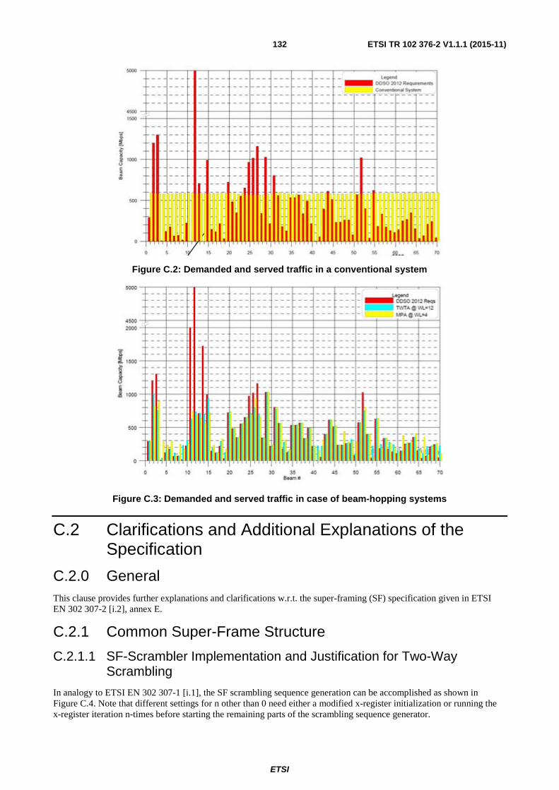
ETSI

ETSI TR 102 376-2 V1.1.1 (2015-11)132

Figure C.2: Demanded and served traffic in a conventional system

Figure C.3: Demanded and served traffic in case of beam-hopping systems

C.2 Clarifications and Additional Explanations of the Specification

C.2.0 General This clause provides further explanations and clarifications w.r.t. the super-framing (SF) specification given in ETSI EN 302 307-2 [i.2], annex E.

C.2.1 Common Super-Frame Structure

C.2.1.1 SF-Scrambler Implementation and Justification for Two-Way Scrambling

In analogy to ETSI EN 302 307-1 [i.1], the SF scrambling sequence generation can be accomplished as shown in Figure C.4. Note that different settings for n other than 0 need either a modified x-register initialization or running the x-register iteration n-times before starting the remaining parts of the scrambling sequence generator.

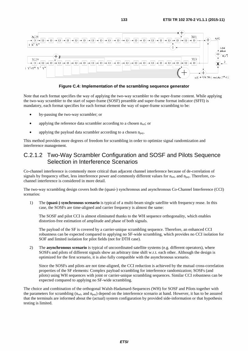
ETSI

ETSI TR 102 376-2 V1.1.1 (2015-11)133

Figure C.4: Implementation of the scrambling sequence generator

Note that each format specifies the way of applying the two-way scrambler to the super-frame content. While applying the two-way scrambler to the start of super-frame (SOSF) preamble and super-frame format indicator (SFFI) is mandatory, each format specifies for each format element the way of super-frame scrambling to be:

• by-passing the two-way scrambler; or

• applying the reference data scrambler according to a chosen nref; or

• applying the payload data scrambler according to a chosen npay.

This method provides more degrees of freedom for scrambling in order to optimize signal randomization and interference management.

C.2.1.2 Two-Way Scrambler Configuration and SOSF and Pilots Sequence Selection in Interference Scenarios

Co-channel interference is commonly more critical than adjacent channel interference because of de-correlation of signals by frequency offset, less interference power and commonly different values for nref, and npay. Therefore, co-channel interference is considered in more detail.

The two-way scrambling design covers both the (quasi-) synchronous and asynchronous Co-Channel Interference (CCI) scenarios:

1) The (quasi-) synchronous scenario is typical of a multi-beam single satellite with frequency reuse. In this case, the SOSFs are time-aligned and carrier frequency is almost the same:

The SOSF and pilot CCI is almost eliminated thanks to the WH sequence orthogonality, which enables distortion-free estimation of amplitude and phase of both signals.

The payload of the SF is covered by a carrier-unique scrambling sequence. Therefore, an enhanced CCI robustness can be expected compared to applying no SF-wide scrambling, which provides no CCI isolation for SOF and limited isolation for pilot fields (not for DTH case).

2) The asynchronous scenario is typical of uncoordinated satellite systems (e.g. different operators), where SOSFs and pilots of different signals show an arbitrary time shift w.r.t. each other. Although the design is optimized for the first scenario, it is also fully compatible with the asynchronous scenario.

Since the SOSFs and pilots are not time-aligned, the CCI reduction is achieved by the mutual cross-correlation properties of the SF elements: Complex payload scrambling for interference randomization; SOSFs (and pilots) using WH sequences with joint or carrier-unique scrambling sequences. Similar CCI robustness can be expected compared to applying no SF-wide scrambling.

The choice and combination of the orthogonal Walsh-Hadamard-Sequences (WH) for SOSF and Pilots together with the parameters for scrambling (nref, and npay) depend on the interference scenario at hand. However, it has to be assured that the terminals are informed about the (actual) system configuration by provided side-information or that hypothesis testing is limited.

ETSI

ETSI TR 102 376-2 V1.1.1 (2015-11)134

Case-Study: (Quasi-) Synchronous CCI of Same Super-Frame Format

In this case, two signals from two beams superimpose quasi synchronously in time and at the same carrier frequency. This is visualized in Figure C.5, where SF format 4 is used for this example. In such a system, a terminal has to be able to apply interference mitigation or cancellation techniques which are based on channel estimates of the different signals. These estimates are derived from reference sequences like SOSF, ST, or pilots, which has to be orthogonal w.r.t. the other signals. In order to exploit the orthogonality of the different WH sequences of the different signals, the interfering signals have to feature the same reference data scrambling nref. However, the payload data has to be as de-correlated as possible, wherefore different values for npay may be used for different signals.

Figure C.5: Scrambling principle in a synchronous interference case to exploit orthogonality, where SF format 4 is used for this example

For system setup it may be beneficial to limit the number of possible values for the WH sequence indices as well as for nref, and npay For faster identification. In the following, an example for a system with 128 beams is provided by means of Table C.2, where the spatial distance between different beam footprints is exploited for re-using values for the WH sequence set (for SOSF, ST, pilots) and npay.

NOTE 1: The depicted WH sequence set numbers in Table C.2 have not to refer directly to a WH sequence index but to a required specification which WH sequences for SOSF, ST, and pilots are applicable per set.

ETSI

ETSI TR 102 376-2 V1.1.1 (2015-11)135

Table C.2: Exemplary setting for a system with 128 beams

WH seq. set n_ref n_payload Assigned beams 0 12 15 0 32 64 96 1 12 16 1 33 65 97 2 12 17 2 34 66 98 3 12 18 3 35 67 99 4 12 19 4 36 68 100 5 12 20 5 37 69 101 6 12 21 6 38 70 102 7 12 22 7 39 71 103 8 12 23 8 40 72 104 9 12 24 9 41 73 105 10 12 25 10 42 74 106 11 12 26 11 43 75 107 12 12 27 12 44 76 108 13 12 28 13 45 77 109 14 12 29 14 46 78 110 15 12 30 15 47 79 111 16 12 31 16 48 80 112 17 12 32 17 49 81 113 18 12 33 18 50 82 114 19 12 34 19 51 83 115 20 12 35 20 52 84 116 21 12 36 21 53 85 117 22 12 37 22 54 86 118 23 12 38 23 55 87 119 24 12 39 24 56 88 120 25 12 40 25 57 89 121 26 12 41 26 58 90 122 27 12 42 27 59 91 123 28 12 43 28 60 92 124 29 12 44 29 61 93 125 30 12 45 30 62 94 126 31 12 46 31 63 95 127

According to this approach, 32 different signals on the same carrier can be distinguished, because all use the same (exemplary) reference data scrambling index nref = 12. The terminal acquisition may be:

1) Terminal identifies SOSF/ST/Pilot sequence set via testing 32 hypothesis, which refers to the first column in Table C.2. In case of format 4, 270 symbols SOSF + 90 symbols ST + 36 pilot symbols = 396 symbols can be used for WH sequence set detection.

2) Applicable payload scrambling index npay is deduced from Table C.2.

NOTE 2: There is a unique value for npay per WH sequence set number in the exemplary setting, wherefore the SFFI structure can also be exploited during acquisition phase 1 to enhance the detection probability, see clause C.3. This would correspond to an effective amount of 495 symbols for detection of SOSF & SFFI and thus in total: 495 symbols SOSF&SFFI + 90 symbols ST + 36 pilot symbols = 621 symbols.

3) Identification of the actual beam, where the terminal is located, can be accomplished e.g. by some payload content like a configuration and EPG stream.

Unfortunately, it is likely that the superimposing signals are not perfectly synchronous, i.e. quasi-synchronous w.r.t. alignment in time of a few symbols offset. Then, the orthogonality cannot be exploited in a straight forward way. Reasons for non-synchronous signals of two beams could be:

• Different satellites

• Different gateways

• Same gateway, but non-phase-stable synchronized modulators

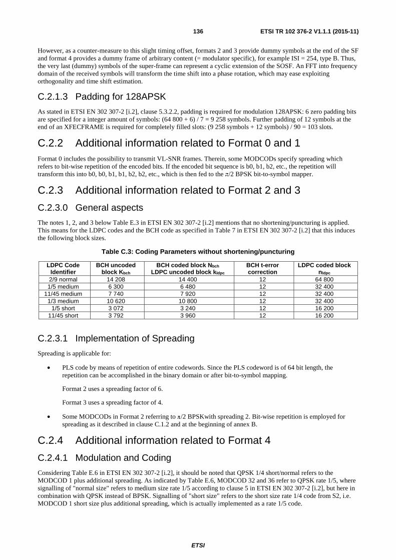
ETSI

ETSI TR 102 376-2 V1.1.1 (2015-11)136

However, as a counter-measure to this slight timing offset, formats 2 and 3 provide dummy symbols at the end of the SF and format 4 provides a dummy frame of arbitrary content (= modulator specific), for example ISI = 254, type B. Thus, the very last (dummy) symbols of the super-frame can represent a cyclic extension of the SOSF. An FFT into frequency domain of the received symbols will transform the time shift into a phase rotation, which may ease exploiting orthogonality and time shift estimation.

C.2.1.3 Padding for 128APSK

As stated in ETSI EN 302 307-2 [i.2], clause 5.3.2.2, padding is required for modulation 128APSK: 6 zero padding bits are specified for a integer amount of symbols: (64 800 + 6) / 7 = 9 258 symbols. Further padding of 12 symbols at the end of an XFECFRAME is required for completely filled slots: (9 258 symbols + 12 symbols) / 90 = 103 slots.

C.2.2 Additional information related to Format 0 and 1 Format 0 includes the possibility to transmit VL-SNR frames. Therein, some MODCODs specify spreading which refers to bit-wise repetition of the encoded bits. If the encoded bit sequence is b0, b1, b2, etc., the repetition will transform this into b0, b0, b1, b1, b2, b2, etc., which is then fed to the π/2 BPSK bit-to-symbol mapper.

C.2.3 Additional information related to Format 2 and 3

C.2.3.0 General aspects

The notes 1, 2, and 3 below Table E.3 in ETSI EN 302 307-2 [i.2] mentions that no shortening/puncturing is applied. This means for the LDPC codes and the BCH code as specified in Table 7 in ETSI EN 302 307-2 [i.2] that this induces the following block sizes.

Table C.3: Coding Parameters without shortening/puncturing

LDPC Code Identifier

BCH uncoded block Kbch

BCH coded block Nbch LDPC uncoded block kldpc

BCH t-error correction

LDPC coded block nldpc

2/9 normal 14 208 14 400 12 64 800 1/5 medium 6 300 6 480 12 32 400

11/45 medium 7 740 7 920 12 32 400 1/3 medium 10 620 10 800 12 32 400

1/5 short 3 072 3 240 12 16 200 11/45 short 3 792 3 960 12 16 200

C.2.3.1 Implementation of Spreading

Spreading is applicable for:

• PLS code by means of repetition of entire codewords. Since the PLS codeword is of 64 bit length, the repetition can be accomplished in the binary domain or after bit-to-symbol mapping.

Format 2 uses a spreading factor of 6.

Format 3 uses a spreading factor of 4.

• Some MODCODs in Format 2 referring to π/2 BPSKwith spreading 2. Bit-wise repetition is employed for spreading as it described in clause C.1.2 and at the beginning of annex B.

C.2.4 Additional information related to Format 4

C.2.4.1 Modulation and Coding

Considering Table E.6 in ETSI EN 302 307-2 [i.2], it should be noted that QPSK 1/4 short/normal refers to the MODCOD 1 plus additional spreading. As indicated by Table E.6, MODCOD 32 and 36 refer to QPSK rate 1/5, where signalling of "normal size" refers to medium size rate 1/5 according to clause 5 in ETSI EN 302 307-2 [i.2], but here in combination with QPSK instead of BPSK. Signalling of "short size" refers to the short size rate 1/4 code from S2, i.e. MODCOD 1 short size plus additional spreading, which is actually implemented as a rate 1/5 code.

ETSI

ETSI TR 102 376-2 V1.1.1 (2015-11)137

The Note 1 below Table E.6 in ETSI EN 302 307-2 [i.2]mentions that no shortening/puncturing is applied. This means for the medium size rate 1/5 code using the BCH code as specified in Table 7 in ETSI EN 302 307-2 [i.2], which leads to the following block sizes:

Table C.4: Coding Parameters for medium FECFRAME nldpc = 32 400 w/o shortening/puncturing

LDPC Code Identifier

BCH uncoded block Kbch

BCH coded block Nbch LDPC uncoded block kldpc

BCH t-error correction

LDPC coded block nldpc

1/5 6 300 6 480 12 32 400

In Table E.8, only normal and short size is considered. Concerning the MODCODs 32 and 36, the calculation w.r.t. the medium size XFECFRAMEs are as follows.

Table C.5: XFECFRAME lengths in CUs according to MOD, SPREAD, and size

Modulation bit/symbol 2 2 Spreading 5 2 CUs, Medium XFECFRAME 960 (see note) 384 (see note) CUs, Short XFECFRAME 480 (see note) 192 (see note) Num. MOD/COD/Spread, u0 = 0 32 36 NOTE: XFECFRAMEs with SPREAD > 1 contain additional pilot

SLOTs, which are included in the length calculation.

C.2.4.2 Implementation of Spreading

In Format 4, spreading is detailed in annex E of ETSI EN 302 307-2 [i.2], clause E.3.6.6, which refers to application of spreading by repeating entire codewords/frames.

C.2.4.3 VL-SNR operation in connection with CCM/ACM/VCM

The target SNR or robustness is indicated by the PLH protection level signalled by the SFH. For ACM/VCM operation below 0 dB SNR, it is recommended to use SF-pilots ON. In case of a VL-SNR CCM, i.e. PLH protection levels 1 or 2, SF-pilots are not required because of constantly present VL-SNR-pilots. A receiver that detects PLH protection level 1 or 2 in combination with SF-pilots off may assume a constant presence VL-SNR-pilots, i.e. only spread MODCODs are expected to be decodable. Note that the VL-SNR-pilots are inserted every 15 payload slots AND at the very end of the PLFRAME.

C.2.4.4 Use of SID/ISI/TSN of the PLH

The PLH of format 4 always signals the SID or ISI, which should correspond to the value in MATYPE2. However, MATYPE2 can also be used as ISI_substream_ID, which is the case if the ISI in PLH and MATYPE2 is different. E.g. for SD and HD-extension substreams and stereo-Audio-stream and Surround-Audio-stream. In total, 254 ISI x 256 substream_IDs = 65024 different streams/ wide-band users can be distinguished.

C.2.4.5 Application of Dummy-Frames

Format 4 provides various types of dummy frames with different signalling:

• Convential Dummy-Frame indicated by MODCOD 0.

• Dummy frames with deterministic content indicated by ISI = 255, where the MODCOD determines the modulation and size.

Type A (signalled by short size): short XFECFRAME length.

Type B (signalled by normal size): normal XFECFRAME length but terminated with end of the actual super-frame.

ETSI

ETSI TR 102 376-2 V1.1.1 (2015-11)138

• Dummy frames with arbitrary content indicated by ISI = 254, where the MODCOD determines the modulation and size.

Type A (signalled by short size): short XFECFRAME length.

Type B (signalled by normal size): normal XFECFRAME length but terminated with end of the actual super-frame.

From this definition, a conflict arises if MODCOD 0 is used in combination with ISI = 255 or 254. Therefore, the following hierarchy is proposed: 1. MODCOD and 2. ISI. In consequence, MODCOD 0 always refers to the conventional dummy frame definition irrespective of the ISI and normal/short size.

If demanded, there is a way to introduce a Cyclic Prefix w.r.t. the SOSF at the end of the super-frame, which may be required in quasi-synchronous CCI scenarios, see clause C.1.1.2. For this case, use the dummy frame with arbitrary content by setting ISI = 254. To limit overhead, normal size = type B may be sufficient to terminate the dummy frame with the end of the super-frame. The modulator can pre-calculate the required symbols, their position in the dummy frame and their pre-rotation to compensate for the payload data scrambler. Note that the last SF-pilot, if present, concludes the super-frame.

C.2.4.6 PLFRAME Mapping into Super-Frame

The main characteristics of the mapping of PLFRAMEs into super-frames are:

• Each XFECFRAME is preceded by a PLH, which forms a PLFRAME.

• PLFRAMEs have no alignment with super-frames except of the CU grid.

• All PLFRAMEs (including spread PLFRAMEs with the extra pilot CUs) are in length a multiple of CUs.

• Individual PLFRAMEs can span over more than one super-frame.

For the following illustrations, two exemplary PLFRAMEs are considered: Either normal-size XFECFRAME with 32APSK (= 144 CUs) or short-size XFECFRAME with QPSK and spreading 2 (= 192 CUs including 12 extra pilot CUs).

Mapping of PLFRAMEs into Super-Frames (Without Spreading)

In Figure C.6, an exemplary mapping of PLFRAMEs into super-frame k is shown, where a fixed XFECFRAME length of 144 CUs has been used, while for the generalized case, any XFECFRAME length can be accommodated per XFECFRAME.

The red dashed arrow refers to the PLH pointer provided by the SFH of Super-frame k:

CU number 31 (one-based counting) = pointer value [00000011110] (zero-based signalling)

Figure C.6: Mapping of PLFRAMEs into super-frames (standard PLH protection)

Furthermore, standard PLH protection has been used in this example, i.e. a PLH of length 2 CUs = 180 symbols. Instead, the high efficiency protection with a PLH length of 1 CU = 90 symbols could have been applied due to purely 32APSK-modulated PLFRAMEs.

ETSI

ETSI TR 102 376-2 V1.1.1 (2015-11)139

Mapping of PLFRAMEs into super-frames (with spreading)

In Figure C.7, an exemplary mapping of PLFRAMEs into super-frame k is shown, where XFECFRAME n+1 requires spreading 2. In this example, the spread XFECFRAME length is 192 CUs with 180 payload CUs and 12 extra pilot CUs, whereas all other unspread XFECFRAMEs have still size 144 CUs. All PLHs of this super-frame have to feature robust protection, i.e. spreading 2.

Figure C.7: Application of spreading to a single PLFRAME within one super-frame

The key idea for the efficient support of spreading within one super-frame is:

• The SFH contains the information on whether PLH spreading is applied to this particular super-frame by means of the 2 bits for PLH protection level.

• If PLH spreading (or protection level) is signalled, ALL PLHs of the entire super-frame have to be repeated by the spread-factor as signalled in the SFH via the PLH protection level, independent on whether an individual XFECFRAME is spread or not. The first PLH, for which the signalled protection level is valid, is indicated by the PLH pointer, see Figure C.8.

• This is the only way how a receiver operating in low SNR regions can continue to track the PLHs until it finds the XFECFRAME which belongs to him.

• Each XFECFRAME, which is required to be spread as indicated in its preceding PLH, has to be repeated spread-factor-times.

NOTE: Mixing the actual spread-factor of XFECFRAMES is possible as long as it is less or equal than the PLH protection level signalled via the SFH, which can be considered as spreading indicator. More specifically, if e.g. the (maximum) PLH spreading-factor of 5 is signalled by the SFH, the XFECFRAMEs can be spread by 1, 2 or 5 according to the signalling in each PLH. This leads in average to less overhead than any static spreading according to the maximum required robustness of the PLHs.

A spread XFECFRAME is also allowed to be split over two super-frames, where spreading (PLH protection) is signalled by the first SFH but not by the consecutive SFH. The receiver has to be aware that also the sequence of PLH repetitions can be interrupted by SOSF + SFFI + SFH + ST or by SF-Pilots, whose occurrence cycle is known and has to be tracked also by the receiver under low SNR conditions. This concept is in line with the aim of avoiding padding for multiplex efficiency, but may add the requirement of further receiver logic compared to padding.

Figure C.8: Different CU allocation cases and applicable PLH protection level signalling

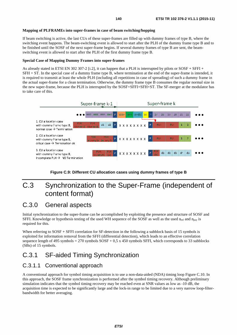
ETSI

ETSI TR 102 376-2 V1.1.1 (2015-11)140

Mapping of PLFRAMEs into super-frames in case of beam switching/hopping

If beam switching is active, the last CUs of these super-frames are filled up with dummy frames of type B, where the switching event happens. The beam-switching event is allowed to start after the PLH of the dummy frame type B and to be finished until the SOSF of the next super-frame begins. If several dummy frames of type B are sent, the beam-switching event is allowed to start after the PLH of the first dummy frame type B.

Special Case of Mapping Dummy Frames into super-frames

As already stated in ETSI EN 302 307-2 [i.2], it can happen that a PLH is interrupted by pilots or SOSF + SFFI + SFH + ST. In the special case of a dummy frame type B, where termination at the end of the super-frame is intended, it is required to transmit at least the whole PLH (including all repetitions in case of spreading) of such a dummy frame in the actual super-frame for a clean termination. Otherwise, the dummy frame type B consumes the regular normal size in the new super-frame, because the PLH is interrupted by the SOSF+SFFI+SFH+ST. The SF-merger at the modulator has to take care of this.

Figure C.9: Different CU allocation cases using dummy frames of type B

C.3 Synchronization to the Super-Frame (independent of content format)

C.3.0 General aspects Initial synchronization to the super-frame can be accomplished by exploiting the presence and structure of SOSF and SFFI. Knowledge or hypothesis testing of the used WH sequence of the SOSF as well as the used nref and npay is required for this.

When referring to SOSF + SFFI correlation for SF-detection in the following a subblock basis of 15 symbols is exploited for information removal from the SFFI (differential detection), which leads to an effective correlation sequence length of 495 symbols = 270 symbols SOSF + 0,5 x 450 symbols SFFI, which corresponds to 33 subblocks (SBs) of 15 symbols.

C.3.1 SF-aided Timing Synchronization

C.3.1.1 Conventional approach

A conventional approach for symbol timing acquisition is to use a non-data-aided (NDA) timing loop Figure C.10. In this approach, the SOSF frame synchronization is performed after the symbol timing recovery. Although preliminary simulation indicates that the symbol timing recovery may be reached even at SNR values as low as -10 dB, the acquisition time is expected to be significantly large and the lock-in range to be limited due to a very narrow loop-filter-bandwidth for better averaging.

ETSI

ETSI TR 102 376-2 V1.1.1 (2015-11)141

Figure C.10: Straight forward approach for timing and SOSF-based super-frame synchronization

In principle, the acquisition strategy is to start the NDA timing loop and activate the SOSF + SFFI - based frame synchronization after the timing recovery has been achieved (e.g. by setting an error threshold or processing certain number of symbols).

After timing loop lock, SOSF-plus-differential-SFFI detection is performed. For a constant probability of false detection Pr(FA) = 10-5, simulation results are shown in Figure C.11 w.r.t. the probability of misdetecting a correlation peak Pr(Missed Peak) for different correlation algorithms versus SNR. Obviously the full correlation algorithm is not robust against frequency offsets, which is why the subblock-based algorithms Abs2 and XCorr perform better.

Figure C.11: Pr(Missed Peak) for SOSF+SFFI detection after timing loop lock (AWGN channel and different relative frequency offsets)

C.3.1.2 SOSF + SFFI Assisted Symbol Timing Recovery

The previous approach has the advantage of a straight forward and low complexity implementation, but is likely to require further enhancements in order to cope with local clock offsets under the VL-SNR. Figure C.12 illustrates a method to use SOSF + SFFI to assist the symbol timing recovery. In this example, an oversampling factor of 2 (two samples per symbol) has been considered. For oversampling two, sampling phase 1 refers to the even sampling indices and phase 2 refers to all odd sampling indices. Then, a sampling frequency offset can be detected and compensated to arrive in the lock-in range of the timing loop.

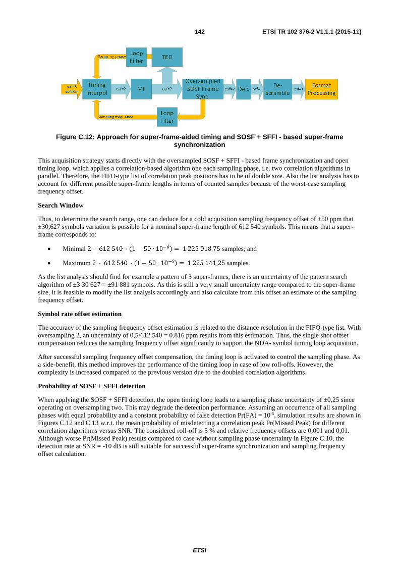
ETSI

ETSI TR 102 376-2 V1.1.1 (2015-11)142

Figure C.12: Approach for super-frame-aided timing and SOSF + SFFI - based super-frame synchronization

This acquisition strategy starts directly with the oversampled SOSF + SFFI - based frame synchronization and open timing loop, which applies a correlation-based algorithm one each sampling phase, i.e. two correlation algorithms in parallel. Therefore, the FIFO-type list of correlation peak positions has to be of double size. Also the list analysis has to account for different possible super-frame lengths in terms of counted samples because of the worst-case sampling frequency offset.

Search Window

Thus, to determine the search range, one can deduce for a cold acquisition sampling frequency offset of ±50 ppm that ±30,627 symbols variation is possible for a nominal super-frame length of 612 540 symbols. This means that a super-frame corresponds to:

• Minimal 2 ⋅ 612540 ⋅ �1 − 50 ∙ 10��� = 1225018,75 samples; and

• Maximum 2 ⋅ 612540 ⋅ �1 − 50 ∙ 10��� = 1225141,25 samples.

As the list analysis should find for example a pattern of 3 super-frames, there is an uncertainty of the pattern search algorithm of ±3⋅30 627 = ±91 881 symbols. As this is still a very small uncertainty range compared to the super-frame size, it is feasible to modify the list analysis accordingly and also calculate from this offset an estimate of the sampling frequency offset.

Symbol rate offset estimation

The accuracy of the sampling frequency offset estimation is related to the distance resolution in the FIFO-type list. With oversampling 2, an uncertainty of 0,5/612 540 = 0,816 ppm results from this estimation. Thus, the single shot offset compensation reduces the sampling frequency offset significantly to support the NDA- symbol timing loop acquisition.

After successful sampling frequency offset compensation, the timing loop is activated to control the sampling phase. As a side-benefit, this method improves the performance of the timing loop in case of low roll-offs. However, the complexity is increased compared to the previous version due to the doubled correlation algorithms.

Probability of SOSF + SFFI detection

When applying the SOSF + SFFI detection, the open timing loop leads to a sampling phase uncertainty of ±0,25 since operating on oversampling two. This may degrade the detection performance. Assuming an occurrence of all sampling phases with equal probability and a constant probability of false detection Pr(FA) = 10-5, simulation results are shown in Figures C.12 and C.13 w.r.t. the mean probability of misdetecting a correlation peak Pr(Missed Peak) for different correlation algorithms versus SNR. The considered roll-off is 5 % and relative frequency offsets are 0,001 and 0,01. Although worse Pr(Missed Peak) results compared to case without sampling phase uncertainty in Figure C.10, the detection rate at SNR = -10 dB is still suitable for successful super-frame synchronization and sampling frequency offset calculation.

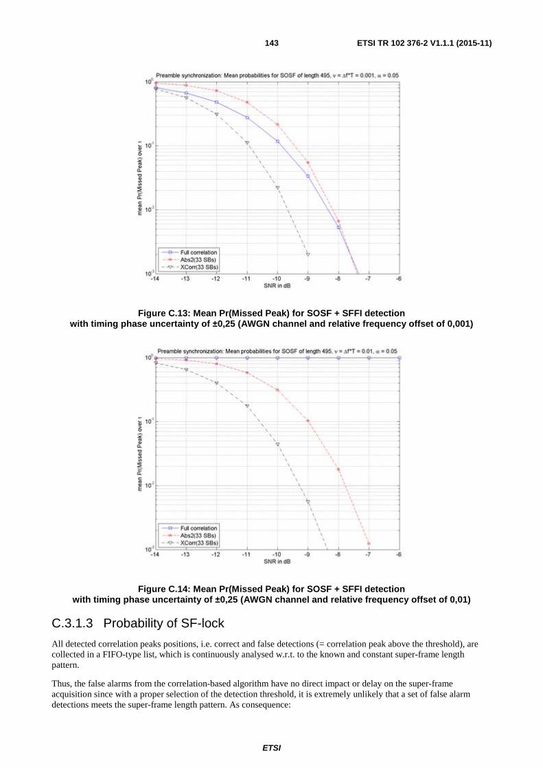
ETSI

ETSI TR 102 376-2 V1.1.1 (2015-11)143

Figure C.13: Mean Pr(Missed Peak) for SOSF + SFFI detection with timing phase uncertainty of ±0,25 (AWGN channel and relative frequency offset of 0,001)

Figure C.14: Mean Pr(Missed Peak) for SOSF + SFFI detection with timing phase uncertainty of ±0,25 (AWGN channel and relative frequency offset of 0,01)

C.3.1.3 Probability of SF-lock

All detected correlation peaks positions, i.e. correct and false detections (= correlation peak above the threshold), are collected in a FIFO-type list, which is continuously analysed w.r.t. to the known and constant super-frame length pattern.

Thus, the false alarms from the correlation-based algorithm have no direct impact or delay on the super-frame acquisition since with a proper selection of the detection threshold, it is extremely unlikely that a set of false alarm detections meets the super-frame length pattern. As consequence:

ETSI

ETSI TR 102 376-2 V1.1.1 (2015-11)144

• The mean super-frame acquisition time is mostly related to the detection of two or more consecutive SOSF/SFFI correlation peaks (an example is shown further below).

• No hypothesis tree is required as in PLFRAME acquisition of the non-super-framing transmission, which is because of the exploited constant super-frame length.

• The probability to erroneously detect the wrong SF-pattern turn extremely fast to zero with increasing the minimum required number of detected correlation peaks that match the SF-pattern.

Based on the previous considerations on Pr(FA) and Pr(MP), an exemplary consideration for the time to super-frame-lock is made here. The event definition is made:

Announce a SF-lock as soon as a set of correlation peak detections is found in the FIFO-type list, when 3 correlation peaks are identified in the FIFO-type list that are multiples of the nominal super-frame length away from each other plus the uncertainty interval due to potential sampling frequency offset.

When reading a Pr(MP)-value from the diagrams, for example 10��, this means that one out of 10 received SOSFs/SFFIs has not been detected via the threshold comparison. These are independent events, wherefore the following probabilities can be determined from combinatorial considerations:

• ���lock after 3 SOSFs� = �1 − �������� = 0,729

• ���lock after 4 SOSFs� = �1 − �������� ⋅ Pr���� ⋅ 3 = 0,2187

• ���lock after 5 SOSFs� = �1 − �������� ⋅ Pr����� ⋅ 6 = 0,0437

• ���lock after SOSFs� = �1 − �������� ⋅ Pr������� ⋅ − 1

2�

As it is of equal probability where to start searching for correlation peaks within the first super-frame, the ���lockafter3SOSFs�refers to a mean acquisition time of 2,5 ⋅ ��� and all further probabilities to (� − 0,5) ⋅ ���, where ��� is the duration of a super-frame. Thus, one can calculate the mean time to SF-lock according to:

��(SF-lock) = ��� ⋅��� − 0.5� ⋅ Pr�lock after � SOSFs����

.

With the introduced values, it result with our example at ��(SF-lock)/��� = 2,833 with (computed based on the first 1000 terms in the summation) super-frames for this calculation. Using Pr(MP) as input parameter, the mean time to lock results by calculation, see Figure C.15.

Figure C.15: Relative mean time to super-frame lock w.r.t. the super-frame duration ��� needing 3 SOSF + SFFIs to successful super-frame lock

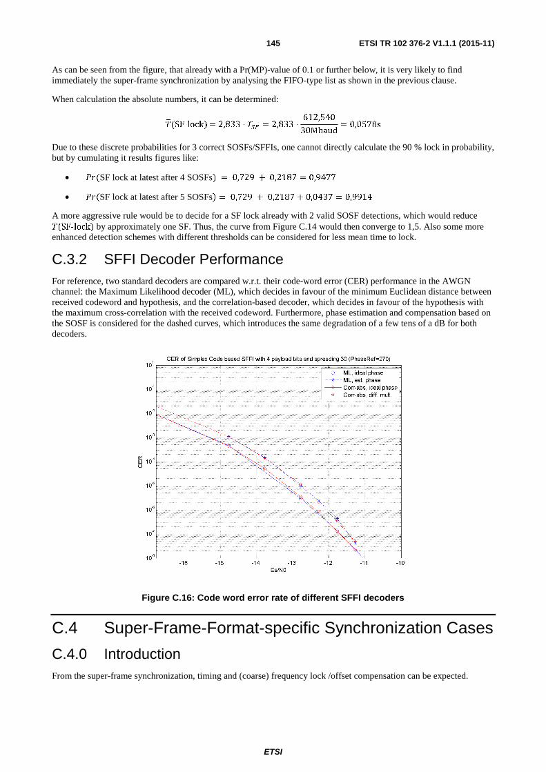
ETSI

ETSI TR 102 376-2 V1.1.1 (2015-11)145

As can be seen from the figure, that already with a Pr(MP)-value of 0.1 or further below, it is very likely to find immediately the super-frame synchronization by analysing the FIFO-type list as shown in the previous clause.

When calculation the absolute numbers, it can be determined:

��(SF-lock��2,833 ⋅ ��� = 2,833 ⋅612,540

30Mbaud= 0,0578s

Due to these discrete probabilities for 3 correct SOSFs/SFFIs, one cannot directly calculate the 90 % lock in probability, but by cumulating it results figures like:

• ��(SF lock at latest after 4 SOSFs) = 0,729 + 0,2187 = 0,9477

• ���SF lock at latest after 5 SOSFs� = 0,729 + 0,2187 + 0,0437 = 0,9914

A more aggressive rule would be to decide for a SF lock already with 2 valid SOSF detections, which would reduce ��(SF-lock) by approximately one SF. Thus, the curve from Figure C.14 would then converge to 1,5. Also some more enhanced detection schemes with different thresholds can be considered for less mean time to lock.

C.3.2 SFFI Decoder Performance For reference, two standard decoders are compared w.r.t. their code-word error (CER) performance in the AWGN channel: the Maximum Likelihood decoder (ML), which decides in favour of the minimum Euclidean distance between received codeword and hypothesis, and the correlation-based decoder, which decides in favour of the hypothesis with the maximum cross-correlation with the received codeword. Furthermore, phase estimation and compensation based on the SOSF is considered for the dashed curves, which introduces the same degradation of a few tens of a dB for both decoders.

Figure C.16: Code word error rate of different SFFI decoders

C.4 Super-Frame-Format-specific Synchronization Cases

C.4.0 Introduction From the super-frame synchronization, timing and (coarse) frequency lock /offset compensation can be expected.

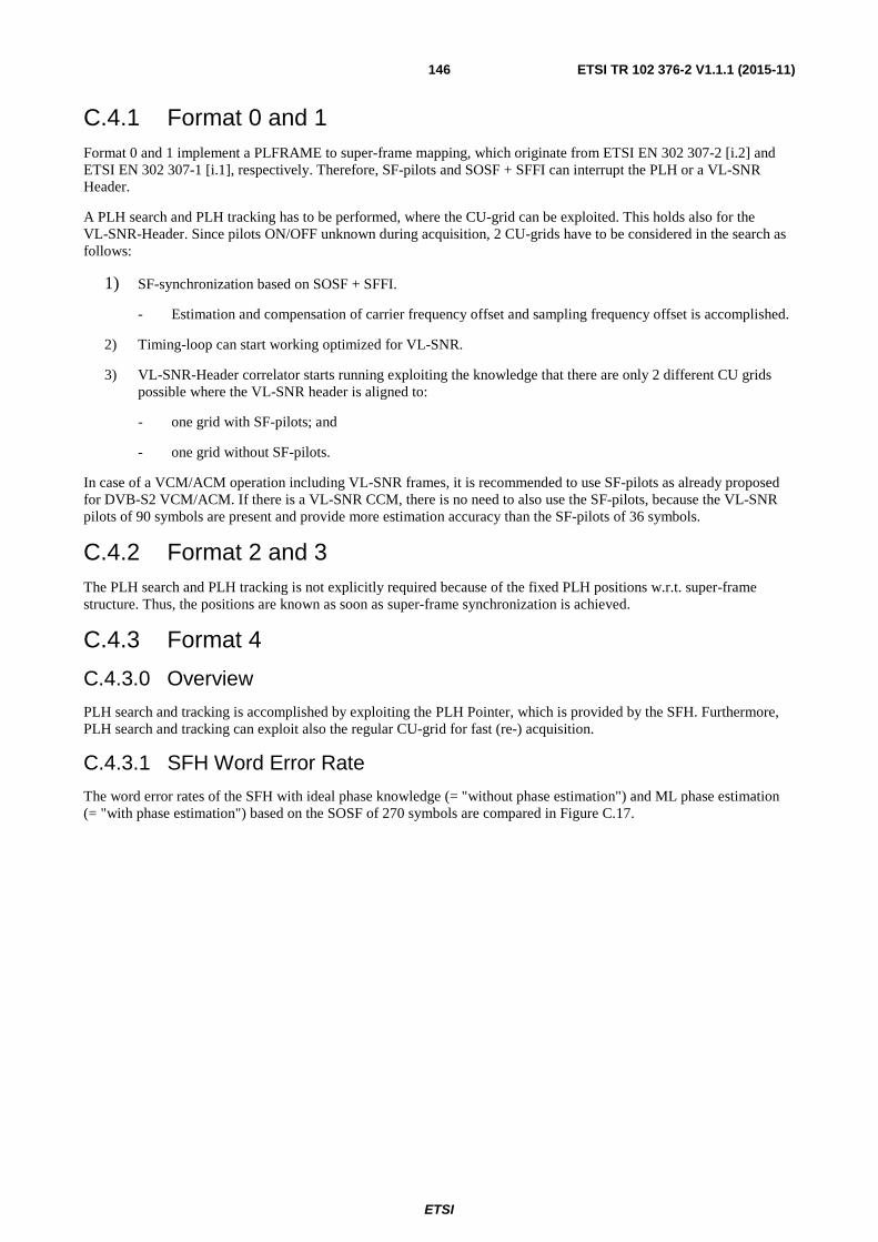
ETSI

ETSI TR 102 376-2 V1.1.1 (2015-11)146

C.4.1 Format 0 and 1 Format 0 and 1 implement a PLFRAME to super-frame mapping, which originate from ETSI EN 302 307-2 [i.2] and ETSI EN 302 307-1 [i.1], respectively. Therefore, SF-pilots and SOSF + SFFI can interrupt the PLH or a VL-SNR Header.

A PLH search and PLH tracking has to be performed, where the CU-grid can be exploited. This holds also for the VL-SNR-Header. Since pilots ON/OFF unknown during acquisition, 2 CU-grids have to be considered in the search as follows:

1) SF-synchronization based on SOSF + SFFI.

- Estimation and compensation of carrier frequency offset and sampling frequency offset is accomplished.

2) Timing-loop can start working optimized for VL-SNR.

3) VL-SNR-Header correlator starts running exploiting the knowledge that there are only 2 different CU grids possible where the VL-SNR header is aligned to:

- one grid with SF-pilots; and

- one grid without SF-pilots.

In case of a VCM/ACM operation including VL-SNR frames, it is recommended to use SF-pilots as already proposed for DVB-S2 VCM/ACM. If there is a VL-SNR CCM, there is no need to also use the SF-pilots, because the VL-SNR pilots of 90 symbols are present and provide more estimation accuracy than the SF-pilots of 36 symbols.

C.4.2 Format 2 and 3 The PLH search and PLH tracking is not explicitly required because of the fixed PLH positions w.r.t. super-frame structure. Thus, the positions are known as soon as super-frame synchronization is achieved.

C.4.3 Format 4

C.4.3.0 Overview

PLH search and tracking is accomplished by exploiting the PLH Pointer, which is provided by the SFH. Furthermore, PLH search and tracking can exploit also the regular CU-grid for fast (re-) acquisition.

C.4.3.1 SFH Word Error Rate

The word error rates of the SFH with ideal phase knowledge (= "without phase estimation") and ML phase estimation (= "with phase estimation") based on the SOSF of 270 symbols are compared in Figure C.17.

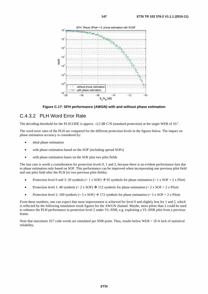
ETSI

ETSI TR 102 376-2 V1.1.1 (2015-11)147

Figure C.17: SFH performance (AWGN) with and without phase estimation

C.4.3.2 PLH Word Error Rate

The decoding threshold for the PLSCODE is approx. -3,5 dB C/N (standard protection) at the target WER of 10-7.

The word error rates of the PLH are compared for the different protection levels in the figures below. The impact on phase estimation accuracy is considered by:

• ideal phase estimation

• with phase estimation based on the SOF (including spread SOFs)

• with phase estimation bases on the SOF plus two pilot fields

The last case is worth a consideration for protection levels 0, 1 and 2, because there is an evident performance loss due to phase estimation only based on SOF. This performance can be improved when incorporating one previous pilot field and one pilot field after the PLH (or two previous pilot fields):

• Protection level 0 and 3: 20 symbols (= 1 x SOF) � 92 symbols for phase estimation (= 1 x SOF + 2 x Pilot)

• Protection level 1: 40 symbols (= 2 x SOF) � 112 symbols for phase estimation (= 2 x SOF + 2 x Pilot)

• Protection level 2: 100 symbols (= 5 x SOF) � 172 symbols for phase estimation (= 5 x SOF + 2 x Pilot)

From these numbers, one can expect that most improvement is achieved for level 0 and slightly less for 1 and 2, which is reflected by the following simulation result figures for the AWGN channel. Maybe, more pilots than 2 could be used to enhance the PLH performance in protection level 2 under VL-SNR, e.g. exploiting a VL-SNR pilot from a previous frame.

Note that maximum 1E7 code words are simulated per SNR point. Thus, results below WER = 1E-6 lack of statistical reliability.

ETSI

ETSI TR 102 376-2 V1.1.1 (2015-11)148

Figure C.18: WER performance of a PLH decoder for protection level 0 (= standard protection, BPSK, Spread 1)

Figure C.19: WER performance of a PLH decoder for protection level 1 (BPSK, Spread 2)

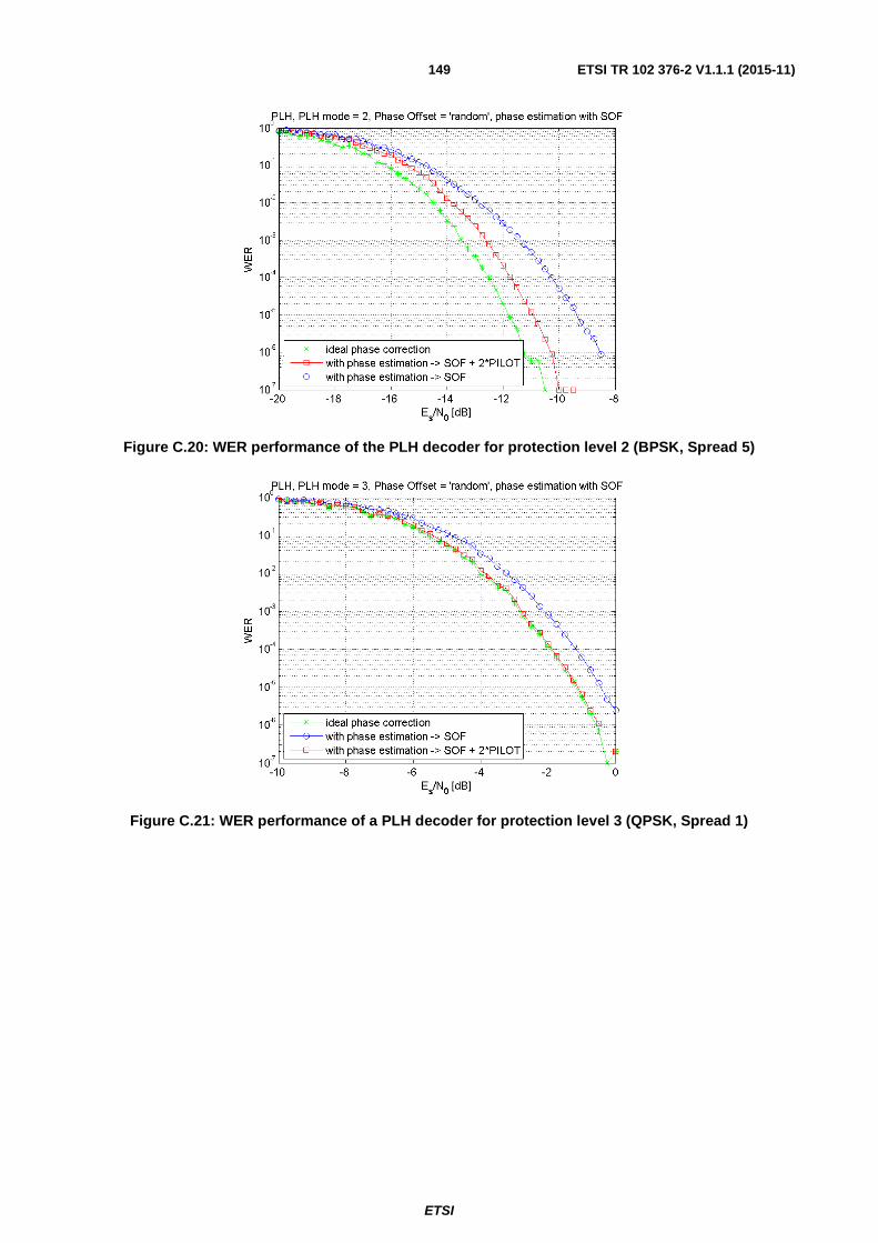
ETSI

ETSI TR 102 376-2 V1.1.1 (2015-11)149

Figure C.20: WER performance of the PLH decoder for protection level 2 (BPSK, Spread 5)

Figure C.21: WER performance of a PLH decoder for protection level 3 (QPSK, Spread 1)

ETSI

ETSI TR 102 376-2 V1.1.1 (2015-11)150

C.5 Example of Exploitation of the Superframing Structure: Precoding in Broadband Interactive Networks

C.5.1 System Elements for Applying Precoding in Multibeam High Throughput Systems

C.5.1.0 General description

Because of the limited fixed satellite service (FSS) spectrum available to broadband systems operating predominantly at Ka-band, increasing the frequency re-use amid the multiple spot beams of High Throughput Satellite (HTS) systems is the main avenue for substantially improving capacity and reducing the offered cost per bit. Current large HTS systems achieving a throughput of more than 100 Gbit/s typically split the available system bandwidth in two frequency bands and two orthogonal polarizations generating the so-called four colour beam pattern across the coverage area. Broadband telecom interactive satellite systems providing multi-beam coverage can substantially increase the available system bandwidth by re-using as much as possible the available spectrum among the spot beams. Nevertheless, increasing the frequency re-use leads to a high increase in intra-system interference between the co-channel beams, which renders the use of additional spectrum futile.

To address the issue of high interbeam interference in aggressive frequency re-use multi-beam configurations, joint processing of the signals intended to the different beams can be carried out at the transmitter (usually the gateway or hub) for interference management. This processing, referred to hereinafter under the generic term precoding, "reverts' the impact of the satellite RF channel and interferences. This way the additional spectrum can be exploited and a much higher system capacity can be delivered compared to existing systems. A precondition for efficient forward link precoding is that the receivers (user terminals, UTs) provide high quality reports of their channel conditions (amplitude and phase) back to the transmitter (gateway, GW) that is responsible for deriving the appropriate precoding matrix.

Various flavours of precoding have been already adopted and are in use in terrestrial cellular radio standards such as the LTE (Long Term Evolution) and LTE-Advanced, falling under the broad term multi-user multiple-input multiple-output (MU-MIMO) techniques. The studies on precoding in a fixed satellite system have been mainly focused with evaluating various linear and non-linear precoding techniques over the multibeam satellite channel in order to assess which technique comes closer to the optimum dirty paper coding (DPC) bound [i.28]. In terms of choice of precoding techniques, it turns out that simple linear techniques already grasp the largest part of the potential multi-user gains with manageable complexity and deliver improvements that at least double the throughput of existing systems ETSI EN 302 307-1 [i.1].

The algorithms needed for precoding to be applied over DVB-S2X need to tackle the situation when each data stream transmitted from an antenna feed towards the spot beam on ground is addressed to multiple UTs and is acting as a container of their data to provide a high degree of statistical multiplexing within the physical layer frame. And the DVB-S2X superframe is one practical example for pursuing such a precoding approach. As a consequence of this framing approach, conventional precoding algorithms addressing a single UT per beam are no longer feasible and precoding algorithms addressing multiple satellite terminals with a single precoding matrix are required. Herein, this type of precoding will be referred to interchangeably as multicast precoding or frame based precoding.

C.5.1.1 System Model & Payload Resources

Figure C.22 illustrates an exemplary satellite communication system that includes a satellite, one or more gateways (GWs) and a high number of UTs and is designed to provide broadband interactive services to a specific coverage area. The satellite is located in the geostationary orbit. Typically, the satellite payload will be transparent: i.e. the payload only frequency translates and amplifies the signals received on the uplink before routing them to the appropriate downlink beam.

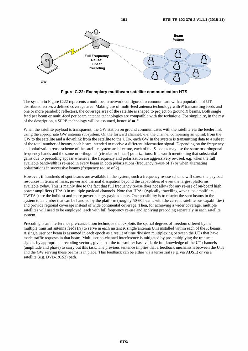
ETSI

ETSI TR 102 376-2 V1.1.1 (2015-11)151

Figure C.22: Exemplary multibeam satellite communication HTS

The system in Figure C.22 represents a multi beam network configured to communicate with a population of UTs distributed across a defined coverage area. Making use of multi-feed antenna technology with N transmitting feeds and one or more parabolic reflectors, the coverage area of the satellite is shaped to project on ground K beams. Both single feed per beam or multi-feed per beam antenna technologies are compatible with the technique. For simplicity, in the rest of the description, a SFPB technology will be assumed, hence � = �.

When the satellite payload is transparent, the GW station on ground communicates with the satellite via the feeder link using the appropriate GW antenna subsystem. On the forward channel, -i.e. the channel comprising an uplink from the GW to the satellite and a downlink from the satellite to the UTs-, each GW in the system is transmitting data to a subset of the total number of beams, each beam intended to receive a different information signal. Depending on the frequency and polarization reuse scheme of the satellite system architecture, each of the � beams may use the same or orthogonal frequency bands and the same or orthogonal (circular or linear) polarizations. It is worth mentioning that substantial gains due to precoding appear whenever the frequency and polarization are aggressively re-used, e.g. when the full available bandwidth is re-used in every beam in both polarizations (frequency re-use of 1) or when alternating polarizations in successive beams (frequency re-use of 2).

However, if hundreds of spot beams are available in the system, such a frequency re-use scheme will stress the payload resources in terms of mass, power and thermal dissipation beyond the capabilities of even the largest platforms available today. This is mainly due to the fact that full frequency re-use does not allow for any re-use of on-board high power amplifiers (HPAs) in multiple payload channels. Note that HPAs (typically travelling wave tube amplifiers, TWTAs) are the bulkiest and more power hungry payload units. One possibility is to restrict the spot beams in the system to a number that can be handled by the platform (roughly 50-60 beams with the current satellite bus capabilities) and provide regional coverage instead of wide continental coverage. Then, for achieving a wider coverage, multiple satellites will need to be employed, each with full frequency re-use and applying precoding separately in each satellite system.

Precoding is an interference pre-cancelation technique that exploits the spatial degrees of freedom offered by the multiple transmit antenna feeds (N) to serve in each instant K single antenna UTs installed within each of the K beams. A single user per beam is assumed in each epoch as a result of time division multiplexing between the UTs that have made traffic requests in that beam. Multiuser co-channel interference is mitigated by pre-multiplying the transmit signals by appropriate precoding vectors, given that the transmitter has available full knowledge of the UT channels (amplitude and phase) to carry out this task. The previous sentence implies that a feedback mechanism between the UTs and the GW serving these beams is in place. This feedback can be either via a terrestrial (e.g. via ADSL) or via a satellite (e.g. DVB-RCS2) path.

ETSI

ETSI TR 102 376-2 V1.1.1 (2015-11)152

C.5.1.2 Forming the Channel Matrix

The general input-output analytical expression for the UT in the k-th beam reads as (see note):

�� = �� �+ ��

where �� is a 1 × � vector composed of the complex channel coefficients (formed by antenna gains, propagation losses and phase shifts) between the UT and the N transmit antenna feeds of the satellite, � is a � × 1 vector of transmitted symbols and �� is the independent identically distributed (i.i.d) zero mean additive white Gaussian noise (AWGN) measured at the k-th receive antenna. This baseband block fading model can be described in compact matrix form as:

= !� + "

where the total channel matrix is the ensemble of all UTs vector channels, i.e. ! = #�,��, … ,��,$. To be noted that in case of a transparent payload architecture where the precoding vectors are applied on ground at the GW, the very high performance (large HPA and antenna) of the GW renders the feeder link between the GW and the satellite almost ideal. This enables considering mostly the user link from the satellite to the UTs at least for the amplitudes in the channel matrix.

NOTE: %† Ndenotes the conjugate transpose of matrix (or vector) A.

C.5.1.3 Algorithms for Multicast Precoding

Linear Precoding Techniques

Linear precoding is a multiuser precoding technique that separates user data streams in specific spatial dimensions. The term linear refers to the linear transmit processing, i.e. the precoding matrix. Although not capacity achieving, under specific optimization algorithms like the ones proposed by the present document, linear techniques can perform close to the optimal channel capacity otherwise given by the non-linear DPC [i.28].

Let us denote by &�, '� , (� the unit power symbol, the � × 1 normalized precoding vector and the scaling factor respectively, corresponding to the UT in the k-th beam. The scaling factor is associated to the k-th signal (i.e. information towards the UT in the k-th beam). Since the output of each antenna will depend on all the input signals, the total transmit signal will read as:

� = �)(��

�

'�&� Subsequently, when precoding is employed, the input-output equation will become:

�� = �� )(� '�&� + �� �)(����

'�&� + ��

where the first term of the summation refers to the useful signal and the second to the interferences. The unit norm column vector '� with dimension � × 1 is the precoding vector associated to the UT in the k-th beam, that is the k-th

column of a total precoding matrix * = #','�, … ,'�,$ . The resulting signal-to-noise-plus-interference ratio (SNIR) at the UT is given by:

+�,-� =(�.��'�.�

1 + ∑ (�.��'�.����

ETSI

ETSI TR 102 376-2 V1.1.1 (2015-11)153

When precoding is employed, determining the optimal precoding vectors is tedious. In the next clause, a very common approach is presented that is also exploited by the multicast precoding in the following:

MMSE Precoding

Based on the theory of uplink/downlink duality [i.30], the precoder can be designed as a linear minimum mean square error (MMSE) filter:

* = 01� +!2!3��!

where the optimal power allocation P (diagonal KxK matrix) under per-antenna constraints is given by solving the dual uplink problem. For the system model presented herein, and assuming a single feed per beam payload architecture, always equal power will be allocated to the multiple satellite antenna feeds.

Multicast Precoding

To apply precoding over DVB-S2X, novel linear precoding designs (i.e. derivations of precoding matrix) based on different algorithms are required. The novelty in these algorithms stems from the fact that these precoder designs satisfy a different need, namely provide improved capacity in spite of the precoder being required to accommodate multiple users which are bundled within a frame. The need of such an approach might be arising from the physical layer framing. This approach towards linear precoding, which can be referred to as Multicast Precoding or Frame based Precoding, has not been investigated for terrestrial or satellite systems so far, either because these systems have no such constraint in their physical layer specification or because it has been implicitly assumed as a problem dealt with at a higher layer.

For example, DVB-S2 achieves a large part of its efficiency in broadband interactive point-to-point system by statistically multiplexing multiple UTs belonging to the same beam in each BBFRAME. Specifically, out of the set of UTs that have requested capacity, the scheduler associated with each beam groups the UTs with similar SNIR characteristics into the same BBFRAME so that identical physical layer transmission modes (ModCods) are applied to them. This concept was designed for maximizing the encapsulation efficiency of the long (16k or 64k) physical layer frames due to LDPC (low density parity check) channel coding.

However, from the precoding point of view, this approach to DVB-S2X framing is adding an important practical constraint since it implies that the precoder cannot be designed on a channel by channel (conventional channel based precoding). Rather, a multicast based precoder should be designed based on the multiple UT channels that are encapsulated in the same frame. The difference between a conventional single UT based precoding and a multicast precoding approach can be understood by contrasting Figure C.23 with Figure C.24. Both depict a simplified multibeam satellite system with N = 2 antenna feeds forming K = 2 spot beams on ground. In Figure C.23, a precoding matrix addressing one UT in each beam is calculated and applied over the same time resource, which is the optimal way of applying precoding as it corresponds to a single instant of the channel matrix. On the other hand, for multicast precoding in Figure C.24 the same precoding matrix is kept over multiple UTs (a, b, c) during the frame period Xa and another one during Xb, X = 1,2, that is over different channel matrix instances, which is clearly suboptimal.

Figure C.23: Example of conventional single UT precoding over a system with channel dimensions 2 x 2

ETSI

ETSI TR 102 376-2 V1.1.1 (2015-11)154

Figure C.24: Example of multicast precoding over a system with channel dimensions 2 x 2. All UTs belonging to the same frame (a, b, c) are served by the same precoding matrix

Different algorithms to calculate the multicast precoding matrix are possible and their details can be found in the published literature (see for example ETSI EN 302 307-1 [i.1] and [i.31]). By selecting the UTs based on certain criteria, these linear precoding schemes applied over all channels during a frame period, although suboptimal, achieve substantial precoding gains compared to conventional four color multi-beam systems.

C.5.1.4 Implementation Aspects of Multicast Precoding

The implementation of precoding techniques in broadband interactive satellite systems requires an air interface which supports a number of special features including regular channel framing structure, specific pilots and unique words for synchronization aid as well as a feedback signalling message from the UTs to the GW. All these features have been included in DVB-S2X.

The super-frame structure supports orthogonal Start of Super-Frame (SOSF) and pilot fields by using Walsh- Hadamard sequences. A set of orthogonal sequences can be assigned to co-channel carriers within a multi-spot beam network (a unique sequence per beam). These features allow the UT to estimate the channel responses from the antenna feeds down to its receiver to a very low SNIR value. The beam-specific orthogonal sequence allows the terminal to uniquely associate the channel estimate to the beam index.

The format specifications 2 and 3 of the superframe (the ones to be used for precoding) also foresee an additional precoded pilot field to help amplitude and carrier phase recovery in support of the precoded data detection. A clever multi-level sequence with the same modulation format as the one of the following payload data is used in these pilots in order to ease the receiver synchronization tasks. Another important feature of the formats 2 and 3 of the superframe, is the possibility to maintain constant and aligned (over co-channel carriers) PLFRAME size, using the Bundled PL-FRAME concept by which DVB-S2 codewords with the same MODCOD are conveniently grouped to resort to a regular length framing structure. Users using the same precoding coefficients, are opportunistically scheduled within a Bundled PL-FRAME. The alignment of such frames over different co-channel carriers helps the gateway to reduce its computational burden.

ETSI

ETSI TR 102 376-2 V1.1.1 (2015-11)155

Figure C.25: Periodic procedure for collecting the complex channel gains from the UTs and feeding them back to the GW

Figure C.24 and Figure C.25 describe how the actual implementation of the precoding technique can be carried out for a DVB-S2X based multi-beam networks. In Figure C.24, the main functional tasks to be carried out in support of precoding are depicted. Each UT estimates a number of channel complex coefficients corresponding to the most significant interfering beams (assumed 10-15 in the figure). These complex numbers are signalled back to the GW using the signalling message described in clause E.4 of ETSI EN 302 307-2 [i.2] with a maximum rate of one message every 500 ms. The next clause provides some insight on the end-to-end system effects (payload, RF propagation, terminal) that influence the quality of this estimation process during each estimation period.

In Figure C.25, the functional bock diagram of a DVB-S2X GW modulator supporting precoding is given. The block precoding matrix is applied right after the constellation mapper of the bank of modulators and is activated on all the fields of the DVB-S2X superframe except for the dispersed orthogonal pilots and the start of superframe. The module accepts as an input the precoding matrix coefficients that are repeatedly computed by the GW processor based on the feedbacks that the UTs transmit to the GW through the return link (either satellite or terrestrial-based).

GWY

C

I1 I2

Userterminals estimate the

end-to-end channel frequency response for C,

I1 and I2, i.e. Hi1,Hi2 and Hi3- up to 10~15 interference channel

responses for full frequency –re-use

systems

Hi1, Hi2, ….HiN (N complex numbers):reported on the return channels when significant changes are detected – worst case every ~ 1 sec

in deep fading conditions similarly to the ACM signaling

1

2

3

The GW computes that channel precoding matrix

given the reported channel responses reported by each

terminal in the coverage

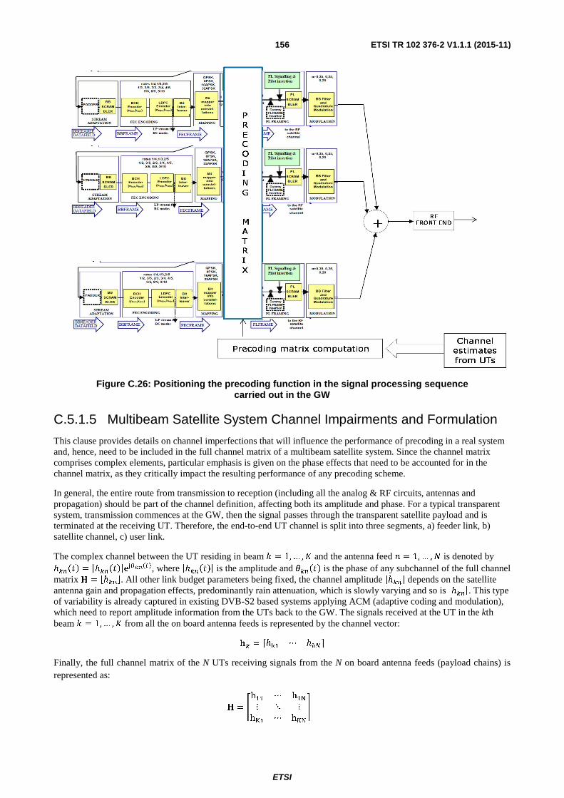
ETSI

ETSI TR 102 376-2 V1.1.1 (2015-11)156

Figure C.26: Positioning the precoding function in the signal processing sequence carried out in the GW

C.5.1.5 Multibeam Satellite System Channel Impairments and Formulation

This clause provides details on channel imperfections that will influence the performance of precoding in a real system and, hence, need to be included in the full channel matrix of a multibeam satellite system. Since the channel matrix comprises complex elements, particular emphasis is given on the phase effects that need to be accounted for in the channel matrix, as they critically impact the resulting performance of any precoding scheme.

In general, the entire route from transmission to reception (including all the analog & RF circuits, antennas and propagation) should be part of the channel definition, affecting both its amplitude and phase. For a typical transparent system, transmission commences at the GW, then the signal passes through the transparent satellite payload and is terminated at the receiving UT. Therefore, the end-to-end UT channel is split into three segments, a) feeder link, b) satellite channel, c) user link.

The complex channel between the UT residing in beam 4 � 1,… , � and the antenna feed � � 1,… , � is denoted by 8���9� � |8���9�|e�������, where |8���9�| is the amplitude and ;���9� is the phase of any subchannel of the full channel matrix < � 08��3. All other link budget parameters being fixed, the channel amplitude |8��| depends on the satellite antenna gain and propagation effects, predominantly rain attenuation, which is slowly varying and so is |8��|. This type of variability is already captured in existing DVB-S2 based systems applying ACM (adaptive coding and modulation), which need to report amplitude information from the UTs back to the GW. The signals received at the UT in the kth beam 4 � 1,… , � from all the on board antenna feeds is represented by the channel vector:

=� � 08� ⋯ 8��3 Finally, the full channel matrix of the N UTs receiving signals from the N on board antenna feeds (payload chains) is represented as:

< � ?h ⋯ h�⋮ ⋱ ⋮h� ⋯ h��C

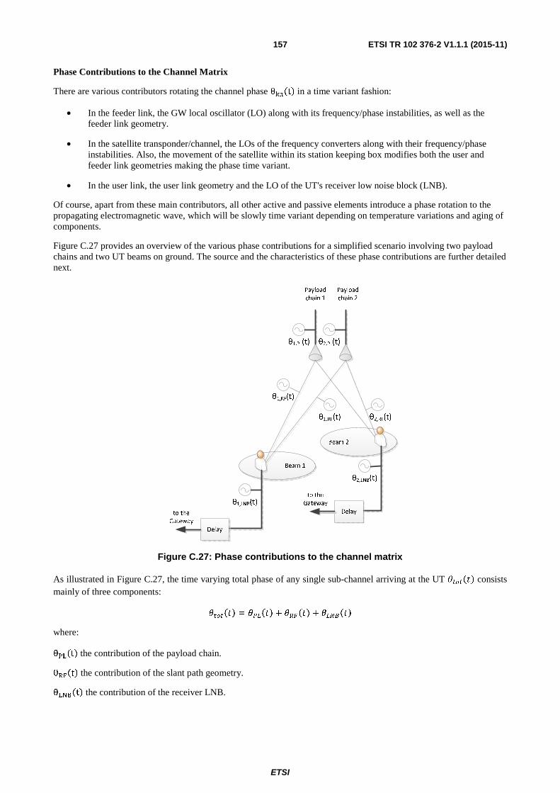
ETSI

ETSI TR 102 376-2 V1.1.1 (2015-11)157

Phase Contributions to the Channel Matrix

There are various contributors rotating the channel phase ��t� in a time variant fashion:

• In the feeder link, the GW local oscillator (LO) along with its frequency/phase instabilities, as well as the feeder link geometry.

• In the satellite transponder/channel, the LOs of the frequency converters along with their frequency/phase instabilities. Also, the movement of the satellite within its station keeping box modifies both the user and feeder link geometries making the phase time variant.

• In the user link, the user link geometry and the LO of the UT's receiver low noise block (LNB).

Of course, apart from these main contributors, all other active and passive elements introduce a phase rotation to the propagating electromagnetic wave, which will be slowly time variant depending on temperature variations and aging of components.

Figure C.27 provides an overview of the various phase contributions for a simplified scenario involving two payload chains and two UT beams on ground. The source and the characteristics of these phase contributions are further detailed next.

Figure C.27: Phase contributions to the channel matrix

As illustrated in Figure C.27, the time varying total phase of any single sub-channel arriving at the UT ;����9� consists mainly of three components:

;����9� = ;� �9� + ;!��9� + ; �"�9� where:

θ#$�t� the contribution of the payload chain.

θ%&�t� the contribution of the slant path geometry.

θ$�'�t� the contribution of the receiver LNB.

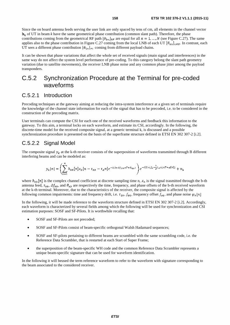
ETSI

ETSI TR 102 376-2 V1.1.1 (2015-11)158

Since the on board antenna feeds serving the user link are only spaced by tens of cm, all elements in the channel vector =� of UT in beam k have the same geometrical phase contribution (common slant path). Therefore, the phase contributions coming from the geometrical RF path 0;��3!� are equal for all � = 1,… ,� (see Figure C.27). The same applies also to the phase contribution in Figure C.27 coming from the local LNB of each UT 0;��3 �". In contrast, each UT sees a different phase contribution 0;��3� coming from different payload chains.

It can be shown that phase variations that affect the whole set of received signals (main signal and interferences) in the same way do not affect the system level performance of pre-coding. To this category belong the slant path geometry variation (due to satellite movements), the receiver LNB phase noise and any common phase jitter among the payload transponders.

C.5.2 Synchronization Procedure at the Terminal for pre-coded waveforms

C.5.2.1 Introduction

Precoding techniques at the gateway aiming at reducing the intra-system interference at a given set of terminals require the knowledge of the channel state information for each of the signal that has to be precoded, i.e. to be considered in the construction of the precoding matrix.

User terminals can compute the CSI for each one of the received waveforms and feedback this information to the gateway. To this aim, a terminal locks on each waveform, and estimate its CSI, accordingly. In the following, the discrete-time model for the received composite signal, at a generic terminal k, is discussed and a possible synchronization procedure is presented on the basis of the superframe structure defined in ETSI EN 302 307-2 [i.2].

C.5.2.2 Signal Model

The composite signal �� at the k-th receiver consists of the superposition of waveforms transmitted through B different interfering beams and can be modeled as:

��[�] = D� ℎ�(0�3�(0� − E�( − E)�3F�*(�+,-���./���)"

(

G F�*(�+(-�/�-��)�./0[�])

+ ��

where ℎ�([�] is the complex channel coefficient at discrete sampling time n, �( is the signal trasmitted through the b-th antenna feed, E�(, HI�(, and ;�( are respectively the time, frequency, and phase offsets of the b-th received waveform at the k-th terminal. Moreover, due to the characteristics of the receiver, the composite signal is affected by the following common impairments: time and frequency drift, i.e. E)�, I)�, frequency offset I��, and phase noise J�[�] In the following, it will be made reference to the waveform structure defined in ETSI EN 302 307-2 [i.2]. Accordingly, each waveform is characterized by several fields among which the following will be used for synchronization and CSI estimation purposes: SOSF and SF-Pilots. It is worthwhile recalling that:

• SOSF and SF-Pilots are not precoded;

• SOSF and SF-Pilots consist of beam-specific orthogonal Walsh Hadamard sequences;

• SOSF and SF-pilots pertaining to different beams are scrambled with the same scrambling code, i.e. the Reference Data Scrambler, that is restarted at each Start of Super Frame;

• the superposition of the beam-specific WH code and the common Reference Data Scrambler represents a unique beam-specific signature that can be used for waveform identification.

In the following it will beused the term reference waveform to refer to the waveform with signature corresponding to the beam associated to the considered receiver.

ETSI

ETSI TR 102 376-2 V1.1.1 (2015-11)159

C.5.2.3 Synchronization Procedure

C.5.2.3.0 General description

Let us consider an indexing function K(L) taking values in the set + = {0,1,2, . . . ,M}, i.e. K(L) ∈ + = {0,1,2, . . . ,M}, L =1,2, . . . ,M, where K(L) = 0 means that the L-th waveform component is not considered in the processing. In order to be able to estimate the CSI to be sent back to the gateway, each receiver can proceed with the following general synchronization/estimation operations:

a) identify the frame boundary, i.e. frame synchronization, for the K(L)-th waveform component, L = 1, . . . ,M;

b) synchronize frequency, phase, and time for the K(L)-th waveform component, L = 1, . . . ,M;

c) perform channel estimation for the K(L)-th waveform component, L = 1, . . . ,M to be sent back to the gateway.

To this aim, the k-th UT:

• performs and applies a coarse frequency estimation by means of a non-data aided estimator on ��0�3, since the frame synchronization procedure is not accounted yet;

• for each waveform K(L), L = 1,2, . . . ,M, performs frame synchronization, if pilot fields or unique words are present in the frame format, to identify frame boundaries. Non-coherent post detection integration can be applied to cope with the residual frequency uncertainty and the time varying phase impairment; For those waveform components for which frame synchronization is not successfully achieved K(L) is set to zero so as to exclude them from the subsequent processing;

• for each waveform �(�),� = 1,2, . . . ,� for which frame synchronization is successfully achieved, performs fine time tracking, phase and frequency tracking, and channel estimation.

A high level block diagram of the synchronization procedure is reported in Figure C.28 with reference the superframe structure described in annex E of ETSI EN 302 307-2 [i.2]. Assuming the same baud rate for all of the received waveforms, two possible implementations are devised depending on the relative delays of the received waveforms. One implementation refers to the case of low data rates for which the received waveforms can be considered "quasi synchronous", i.e. the relative time delays τ�1 are within one symbol time. The second one refers to the complementary case of "non-synchronous" waveforms, i.e. the relative time delays τ�1 may exceed one symbol time.

C.5.2.3.1 Synchronization procedure for "Quasi-Synchronous" Signals

1) Coarse frequency acquisition.

- At the output of this step, coarse frame estimation is available.

2) Matched filtering MF is performed on the composite waveform.

3) Frame synchronization of the reference waveform. Non-coherent post-detection integration is run on the composite signal using SOSF and SF-Pilot fields.

- Frame boundaries are available after this step for the reference waveform. Due to the "quasi-synchronous" assumption this applies also for the, still unknown, interferers waveforms.

4) Time drift estimation. Once a lock is obtained on the reference waveform two successive SOSF fields are used to estimate the timing drift.

- At the output at this step, the estimate of the time drift is available.

5) Time drift compensation. The estimate obtained at the previous step is used to compensate the time drift of the composite signal.

- At the output at this step, the time drift has been reduced to a residual that will be dealt with by the time tracking.

ETSI

ETSI TR 102 376-2 V1.1.1 (2015-11)160

6) Interferer Search. To identify which waveforms contribute to the composite signal, and has therefore to be synchronized and their CSI estimated, a search procedure is run using the SOSF and SF-Pilot fields; being the waveforms "quasi-synchronous" a simple search over the set of possible "signatures" is run with the frame synchronization lock obtained on the reference waveform.

- At the output of this step, the number of detectable interferes and their signatures are available.

7) Time tracking. To refine the time estimation and track time variation a Data Aided time tracking algorithm, e.g., a second order loop tracking circuit, is performed on the reference waveform using the SOSF and SF-pilots fields.

- A fine time estimate is produced for the reference waveform.

8) Time Compensation. The composite waveform is resampled on the basis of the fine time estimate obtained on the reference waveform.

- The common time impairments are compensated relatively to the reference waveform.

9) Reference signal frequency and phase tracking. Using the signature of the reference waveform phase and frequency tracking is performed using SOSF and SF-Pilots.

- Fine frequency and phase estimates are produced relatively to the reference waveform.

10) Frequency and Phase Compensation. The composite waveform is de-rotated on the basis of the fine frequency and phase estimates.

- Common frequency and phase impairments are compensated relatively to the reference waveform.

11) Interferer Time tracking. Time estimates are refined for each interferer waveforms, i.e. those waveforms locked during the Interferer Search, using the corresponding signatures. Notably, thanks to the common impairments compensation on the reference waveform, a simpler first order loop approach can be adopted for the interferers.

- A fine time estimate is produced for each identified interferer waveform.

12) Interferer Time Compensation. For each interferer, the composite waveform is resampled on the basis of the fine time estimate of the interferer.

13) Frequency and phase tracking. For each interferer waveform phase and frequency tracking is performed separately using SOSF and SF-Pilots and the corresponding signature.

14) Channel estimation. For each detected and re-synchronized waveform, the complex channel coefficients are estimated.

C.5.2.3.2 Synchronization procedure for "non-synchronous" Signals

1) Coarse frequency acquisition.

- At the output of this step, coarse frame estimation is available.

2) Matched filtering MF is performed on the composite waveform.

3) Frame synchronization of the reference waveform. Non-coherent post-detection integration is run on the composite signal using SOSF and SF-Pilot fields.

- Frame boundaries are available after this step for the reference waveform. Since for high baud rate the received waveforms cannot be assumed "quasi-synchronous", identification of the frame boundaries for the reference waveform does not entail frame synchronization for the interferer waveforms.

4) Time drift estimation. Once a lock is obtained on the reference waveform two successive SOSF fields are used to estimate the timing drift.

- At the output at this step, the estimate of the time drift is available.

ETSI

ETSI TR 102 376-2 V1.1.1 (2015-11)161

5) Time drift compensation. The estimate obtained at the previous step is used to compensate the time drift of the composite signal.

- At the output at this step, the time drift has been reduced to a residual that will be dealt with by the time tracking.

6) Time tracking. To refine the time estimation and track time variation a Data Aided time tracking algorithm, e.g., a second order loop tracking circuit, is performed on the reference waveform using the SOSF and SF-Pilots fields.

- A fine time estimate is produced for the reference waveform.

7) Time Compensation. The composite waveform is resampled on the basis of the fine time estimate obtained on the reference waveform.

- The common time impairments are compensated relatively to the reference waveform.

8) Reference signal frequency and phase tracking. Using the signature of the reference waveform phase and frequency tracking is performed using SOSF and SF-Pilots.

9) Frequency and Phase Compensation. The composite waveform is de-rotated on the basis of the fine frequency and phase estimates.

- Common frequency and phase impairments are compensated relatively to the reference waveform.

10) Interferer Frame Synchronization. Since incoming waveforms are not time aligned, i.e. they are "non-synchronous", a frame synchronization step is required for each possible interfering waveform, i.e. for each possible interfering signature. It is worthwhile noting that since the maximum time misalignment among the reference waveform and the interfering waveforms is limited to M symbols, where M depends on the baud rate and the maximum relative delay of the incoming waveforms, i.e. the max

1τ�1, the frame synchronization

procedure has to be run on an uncertainty region of [-M,M] symbols centred on the reference waveform lock hypothesis.

- For each tested signature a lock/no-lock status is produced.

11) Interferer Verification procedure. For each signature associated to a possible lock status, a verification test is run of the subsequent superframe.

- For each signature with a lock status, the lock status is confirmed or negated and a set of interferer waveforms is then obtained.

12) Interferer Time tracking. The time lock obtained through the interferer frame synchronization and verification procedure are refined for each identified interferer waveforms, i.e. those waveforms with a confirmed lock status, using the SOSF and SF-Pilots with the corresponding signatures. Notably, thanks to the common impairments compensation on the reference waveform, a simpler first order loop approach can be adopted for the interferers.

- A fine time estimate is produced for each identified interferer waveform.

13) Interferer Time Compensation. For each interferer, the composite waveform is resampled on the basis of the fine time estimate of the interferer.

14) Frequency and phase tracking. For each interferer waveform phase and frequency tracking is performed separately using SOSF and SF-pilots and the corresponding signature.

15) Channel estimation. For each detected and re-synchronized waveform, the complex channel coefficients are estimated.

ETSI

ETSI TR 102 376-2 V1.1.1 (2015-11)162

Figure C.28: Block diagram of synchronization procedure taking place at the UT in a system employing precoding

C.5.2.4 Numerical Examples

C.5.2.4.0 Introduction

In this clause a discussion is reported on the impairments used at the receiver followed by the numerical analysis and performance assessment for the receiver algorithms described in Figure C.28.

C.5.2.4.1 Discussion on impairments

In the following, channel impairments are discussed on the basis of system parameters considerations:

• Common Frequency Offset: according to the channel model of clause 4.4, for DTH broadcasting services the maximum carrier frequency instability is ±5 MHz while for VSAT is ±3 MHz;

• Frequency Drift: as reported in channel model of clause 4.4, using low cost components at the terminal can lead to a time varying frequency offset (drift) of 30 KHz/s;

• Waveform specific Frequency offsets: offsets in frequency are due to on-board frequency conversion of feeder link signals coming from different gateways. The frequency offsets can be assumed to be limited to ±1 Hz and hence their impact can be neglected;

• Waveform specific Timing offset: due to different transponder filter group delay, waveforms pertaining to different beams experienced different delays. The worst case is assumed to be 2 nsec RMS, hence a maximum offset with respect to the reference waveform of ±6 nsec. Considering a symbol rate of 80 MBaud the maximum value for the time offset is within half of the symbol rate, and hence signals can be considered "quasi-synchronous". For baud rate larger than 80 MBaud the maximum time offset is no more limited to one symbol time. For 500 Mbaud, the maximum time offset corresponds to ±3 symbols, i.e. M = 3;

• Phase Offset: due to the time offset a phase offset has to be considered for each incoming waveforms with an uniform distribution on00,2P3;

ETSI

ETSI TR 102 376-2 V1.1.1 (2015-11)163

• Timing Drift: due to the oscillator stability at the user terminal, a timing drift in the order of 100 p.p.m. has to be assumed that corresponds to about 60 symbols in 1 superframe;

• Phase Noise: phase noise is modelled according to channel model of clause 4.4, that provides four Phase Noise masks, two for DTH services and 2 for VSAT services.

C.5.2.4.2 Numerical results

C.5.2.4.2.0 Assuptions

This clause reports an example of the performance of the synchronization chain discussed in the previous clauses for a specific scenario assuming impairments as described above in clause C.5.3.4.1 and a symbol rate of 500 MBaud, because it is the most challenging scenario. The assessment has been obtained through numerical simulation adopting specific algorithms for each step and has to be considered only as an example of the synchronization chain performance and implementation, and not as a reference.

According to the previous discussion, for a symbol rate of 500 Mbaud the system is considered as "non-synchronous" and hence the "Synchronization procedure for non-synchronous Signals" is adopted. In particular, for all of the tested algorithms, the following assumptions hold true:

• the user terminal receives 5 interferer waveforms coming from different beams, plus the reference waveform;

• each waveform is a DVB-S2X waveform as described in annex E of ETSI EN 302 307-2 [i.2];

• the format specification is the Bundled PLFRAMES (64 800 payload size) with SF-Pilots;

• the ratio between the power spectral density of the reference signal and that of the received waveforms, i.e. C/I, is C/I = [0 0 4 8 12 16] dB, where the first value refers to the reference waveform normalized to its own power spectral density;

• the ratio between the power spectral density of a particular interferer waveform and the total amount of interference is given by I/ITOT = [-2,16 -7,52 -12,00 -16,12 -20,18] dB;

• the roll-off factor of the square root raised cosine filter used is 0,05.

C.5.2.4.2.1 Coarse Frequency Acquisition

The algorithm used for the frequency acquisition is the so-called Quadricorrelator algorithm [i.23]. It operates on the overall signal and it is the only non-pilot-assisted algorithm used in the synchronization chain. The parameters used to obtain simulation results showed in Figure C.29 are the following:

• Impairments as specified in clause C.5.3.4.1;

• Loop Bandwidth BLT = 2,7e-8;

• Oversampling factor = 2;

• SNR (for the reference waveform) = -10 dB.

ETSI

ETSI TR 102 376-2 V1.1.1 (2015-11)164

Figure C.29 : Frequency acquisition performance

As Figure C.29 reports, the time required by the algorithm to reach the steady state is about 50 milliseconds. The frequency residual from the estimation operation is characterized by a mean value of 10-4 and a standard deviation of 10-4 normalized to the symbol rate for the considered SNR, which is very low in order to test the performance of the algorithm in the worst case scenario.

C.5.2.4.2.2 Frame Synchronization and Interferer Frame Synchronization

After the reduction of the frequency offset and instabilities and without any fine timing information, frame synchronization can be performed. Non-coherent frame synchronization with 2 hypotheses per symbol is proposed to accomplish this operation. Due to the presence of a residual frequency uncertainty and phase noise, post-detection integration (PDI) technique with the Max Criterion is used [i.24] and [i.25]. In addition, the constant length of the framing structure as in annex E of ETSI EN 302 307-2 [i.2] allows the use of more than one SOSF field and SF-Pilot fields in the synchronization procedure.

Frame synchronization performance and interferer frame synchronization performance in terms of false alarm probability are shown in Figure C.30 for each user of the considered scenario. The simulation parameters are:

• Impairments as specified in clause C.5.3.4.1 plus a residual;

• frequency residuals after the Quadricorrelator algorithm compensation;

• 2 hypothesis per symbol;

• Max Criterion;

• PDI factor used for the SOSF field is 4 so frame synchronization performs non-coherent accumulation over 270/4 symbols;

• Number of super-frame used for PDI is 8;

• Uncertainty region for interferer waveforms is M=3.

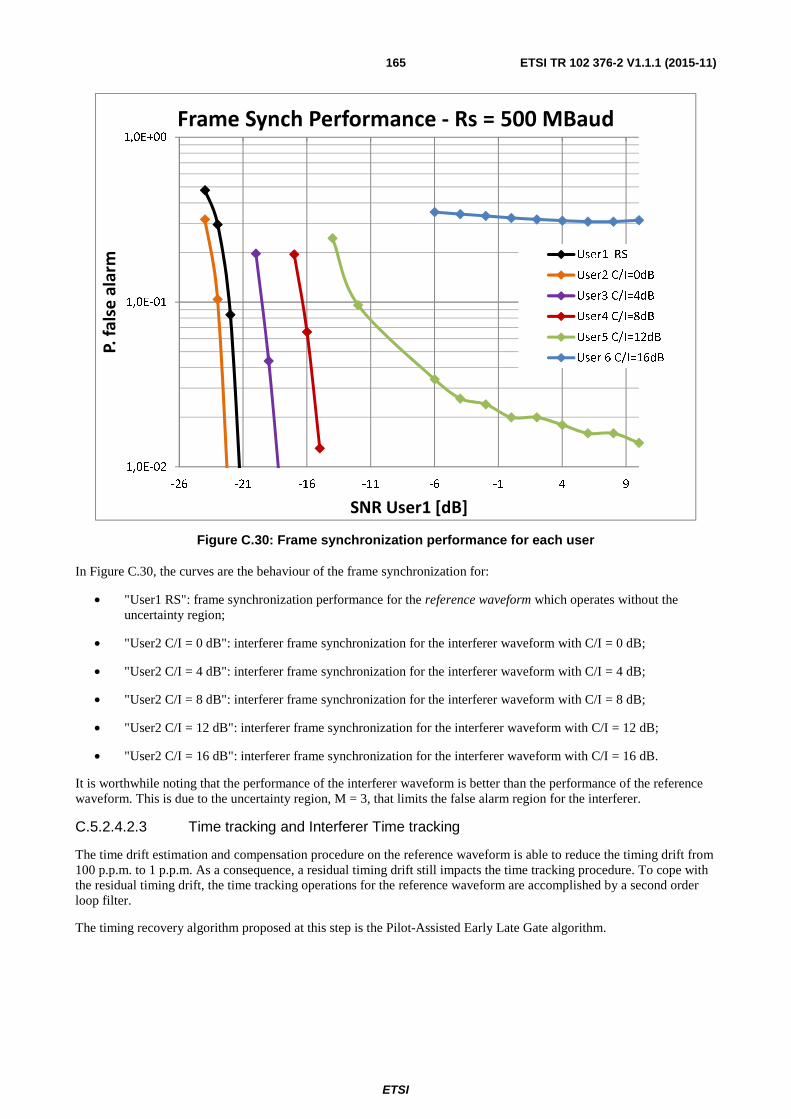
ETSI

ETSI TR 102 376-2 V1.1.1 (2015-11)165

Figure C.30: Frame synchronization performance for each user

In Figure C.30, the curves are the behaviour of the frame synchronization for:

• "User1 RS": frame synchronization performance for the reference waveform which operates without the uncertainty region;

• "User2 C/I = 0 dB": interferer frame synchronization for the interferer waveform with C/I = 0 dB;

• "User2 C/I = 4 dB": interferer frame synchronization for the interferer waveform with C/I = 4 dB;

• "User2 C/I = 8 dB": interferer frame synchronization for the interferer waveform with C/I = 8 dB;

• "User2 C/I = 12 dB": interferer frame synchronization for the interferer waveform with C/I = 12 dB;

• "User2 C/I = 16 dB": interferer frame synchronization for the interferer waveform with C/I = 16 dB.

It is worthwhile noting that the performance of the interferer waveform is better than the performance of the reference waveform. This is due to the uncertainty region, M = 3, that limits the false alarm region for the interferer.

C.5.2.4.2.3 Time tracking and Interferer Time tracking

The time drift estimation and compensation procedure on the reference waveform is able to reduce the timing drift from 100 p.p.m. to 1 p.p.m. As a consequence, a residual timing drift still impacts the time tracking procedure. To cope with the residual timing drift, the time tracking operations for the reference waveform are accomplished by a second order loop filter.

The timing recovery algorithm proposed at this step is the Pilot-Assisted Early Late Gate algorithm.

1,0E-02

1,0E-01

1,0E+00

-26 -21 -16 -11 -6 -1 4 9

P.

fals

e a

larm

SNR User1 [dB]

Frame Synch Performance - Rs = 500 MBaud

User1 RS

User2 C/I=0dB

User3 C/I=4dB

User4 C/I=8dB

User5 C/I=12dB

User 6 C/I=16dB

ETSI

ETSI TR 102 376-2 V1.1.1 (2015-11)166

In Figure C.31, performance for the time tracking algorithm is reported. The simulation parameters used are:

• Impairments as specified in clause C.5.3.4.1;

• frequency residuals after the Quadricorrelator algorithm compensation;

• coarse time synchronization from the frame synchronization procedure;

• timing drift residuals from the time drift estimation and compensation procedure;

• Oversample factor = 4;

• SNR (for the reference waveform) = 10 dB. This value is an example of realistic operative SNR value for precoding.

Figure C.31: Time tracking performance for the reference waveform

The mean and the standard deviation of the timing residuals given by the second order loop filter are respectively 10-2 Ts and 3·10-2 Ts, that highlights the ability of compensating the residual timing drift in the considered conditions.

Timing residuals from the reference waveform are then used to drive the first order loop filters used for interferer time tracking operation.

In Figure C.32 performance for the time tracking algorithms is reported. The simulation parameters used are:

• Impairments as specified in clause C.5.3.4.1;

• frequency residuals after the Quadricorrelator algorithm compensation;

• coarse time synchronization after the frame synchronization procedure;

• timing residuals after the time tracking procedure on the reference signal;

• Oversample factor = 4;

• SNR (for the reference waveform) = 10 dB;

• Loop bandwidth for the time tracking algorithm BLT = 5e-8.

ETSI

ETSI TR 102 376-2 V1.1.1 (2015-11)167

Figure C.32: Interferer time tracking performance for interferer waveforms

Performance in terms of mean and standard deviation of the timing residuals from interferer time tracking algorithm for each interferer waveform are reported in the following:

• "User 2", i.e. interferer waveform with C/I = 0 dB

- Mean = -0,018 Ts; Std = 0,003 Ts;

• "User 3", i.e. interferer waveform with C/I = 4 dB

- Mean = -0,015 Ts; Std = 0,003 Ts;

• "User 4", i.e. interferer waveform with C/I = 8 dB

- Mean = -0,023 Ts; Std = 0,006 Ts;

• "User 5", i.e. interferer waveform with C/I = 12 dB

- Mean = -0,041 Ts; Std = 0,006 Ts;

• "User 6", i.e. interferer waveform with C/I = 16 dB

- Mean = -0,005 Ts; Std = 0,007 Ts;

- It is worthwhile noting that the performance for this interferer waveform has been obtained under a lock status assumption, which is however not verified.

It is worthwhile noting that the time required to reach the steady state depend on the C/I value of a particular interferer waveform due to the correspondent operative very low SNR.

ETSI

ETSI TR 102 376-2 V1.1.1 (2015-11)168

C.5.2.4.2.4 Channel Estimation

After the proper estimation and compensation of all impairments reported in the initial formula, the estimation of the channel coefficient in terms of amplitude and phase is the final operation. The algorithm used to perform this final step is described by the following formula:

��� � ������ � 1�����

��� � � ∙ ��∗� ����

�

��

�

�� �����

∑ ���∑ ��� ���∙��

∗��������

����

Where ��� is the portion of the received overall signal corresponding to the k-th block of the PSF transmitted pilots in one super-frame while NP is the number of successive pilot fields which the estimate is averaged as reported in annex E of ETSI EN 302 307-2 [i.2].

In Table C.6, mean and standard deviation of the amplitude estimation errors (normalized to the corresponded C/I) are reported in logarithmic unit. The SNR used for the simulation, referred to the reference waveform, is 10 dB, as the one used for time tracking and interferer time tracking simulations.

Table C.6 : Mean and standard deviation values of the amplitude errors for the channel coefficients

In Table C.7, mean and standard deviation of the phase estimation errors are reported in degrees.

Table C.7 : Mean and standard deviation values of the phase errors for the channel coefficients

As expected, the estimates for the weakest interferer waveforms are not accurate as the ones obtained for the reference waveform and the interferer waveforms.

Mean and standard deviation for the weakest interferer, the one at C/I = 16 dB, are not reported in the table because it is not possible to achieve the lock status for this waveform in this scenario.

C.5.3 System performance estimation

C.5.3.1 System Overview

It is considered a satellite communication system comprised one or more gateways that are providing communication to a plurality of user beams through one or more satellites. A possible architecture is depicted in Figure C.33.

ETSI

ETSI TR 102 376-2 V1.1.1 (2015-11)169

Figure C.33: Multi-beam satellite system

The two features needed by the system in order to allow precoding are:

1) Presence of a feedback channel for providing to the gateway the channel state information (CSI).

2) Gateways capable of generating the precoding matrix and precode the signals before they are sent through the channel.

In the following the steps to be followed for allowing precoding are listed:

1) The user terminals estimate their channel and feedback the estimates to the gateway. The estimate includes the channel coefficients of the interferers as well.

2) Based on the coefficients and on the traffic requests of the user terminals, the gateway performs the clustering of users according to signal-to-noise plus interference ratio (SNIR) difference. Users with the minimum difference between SNIRs are clustered together.

3) A precoding matrix is computed for the specific cluster of user and maintained for a bundle frame.

4) The precoding matrix is then pre-multiplied to the user symbols in order to pre-distort the signals for minimizing interference.

Precoding is very beneficial for interference limited systems as a multi-beam satellite system employing full frequency reuse. It is a technique that allows mitigating the interference coming from unwanted signals, which in the satellite communication system will mainly be due to co-channel interference caused by neighbouring beams of the considered user terminal.

C.5.3.2 Performance Estimation

C.5.3.2.0 General description of the scenarios

In the following, preliminary performance estimation for precoding in a multi-beam satellite system will be investigated. Two symbol rate scenarios will be taken into account:

1) 80 Mbaud

2) 500 Mbaud

The cases represent two typical scenarios in satellite system, one with limited carrier bandwidth (80 Mbaud) and one with rather extended carrier bandwidth (500 Mbaud).

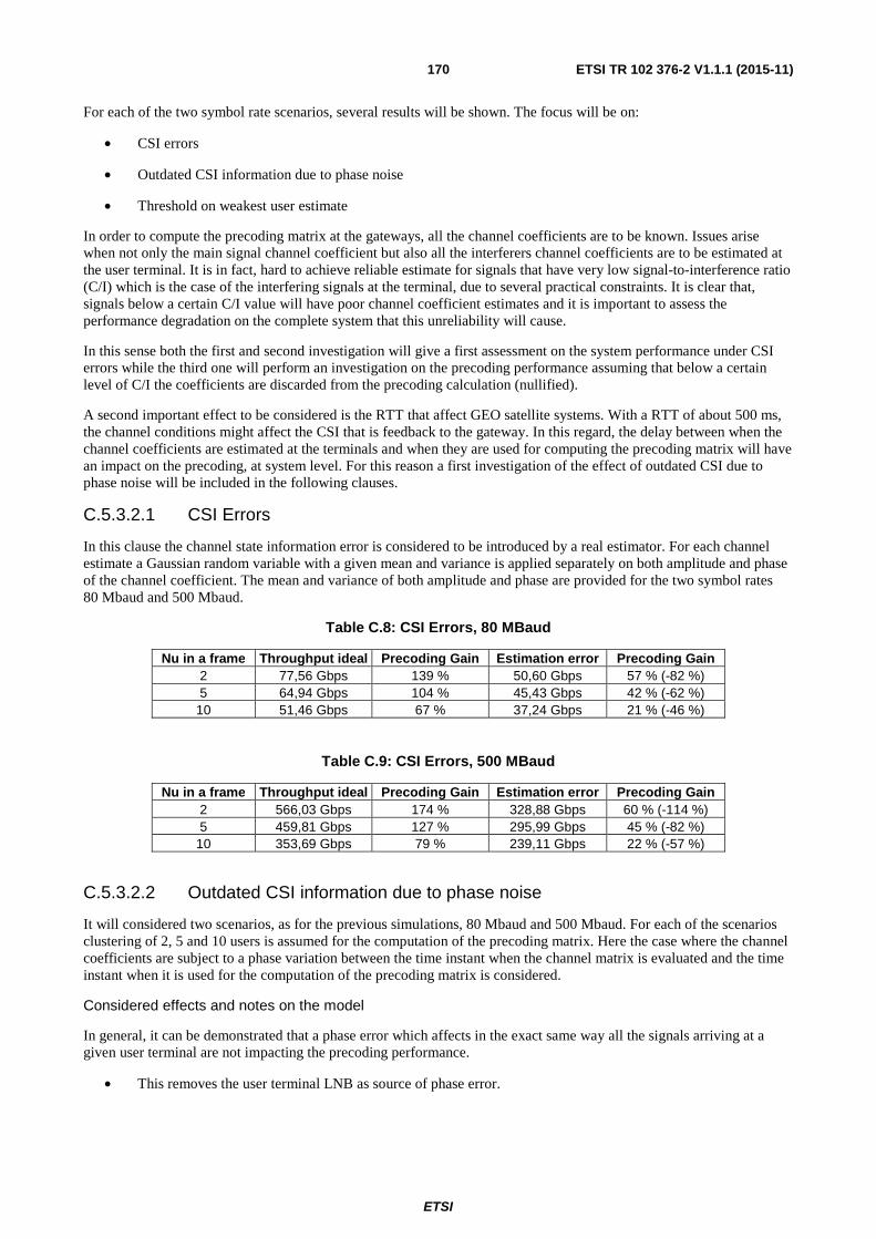
ETSI

ETSI TR 102 376-2 V1.1.1 (2015-11)170

For each of the two symbol rate scenarios, several results will be shown. The focus will be on:

• CSI errors

• Outdated CSI information due to phase noise

• Threshold on weakest user estimate

In order to compute the precoding matrix at the gateways, all the channel coefficients are to be known. Issues arise when not only the main signal channel coefficient but also all the interferers channel coefficients are to be estimated at the user terminal. It is in fact, hard to achieve reliable estimate for signals that have very low signal-to-interference ratio (C/I) which is the case of the interfering signals at the terminal, due to several practical constraints. It is clear that, signals below a certain C/I value will have poor channel coefficient estimates and it is important to assess the performance degradation on the complete system that this unreliability will cause.

In this sense both the first and second investigation will give a first assessment on the system performance under CSI errors while the third one will perform an investigation on the precoding performance assuming that below a certain level of C/I the coefficients are discarded from the precoding calculation (nullified).

A second important effect to be considered is the RTT that affect GEO satellite systems. With a RTT of about 500 ms, the channel conditions might affect the CSI that is feedback to the gateway. In this regard, the delay between when the channel coefficients are estimated at the terminals and when they are used for computing the precoding matrix will have an impact on the precoding, at system level. For this reason a first investigation of the effect of outdated CSI due to phase noise will be included in the following clauses.

C.5.3.2.1 CSI Errors

In this clause the channel state information error is considered to be introduced by a real estimator. For each channel estimate a Gaussian random variable with a given mean and variance is applied separately on both amplitude and phase of the channel coefficient. The mean and variance of both amplitude and phase are provided for the two symbol rates 80 Mbaud and 500 Mbaud.

Table C.8: CSI Errors, 80 MBaud

Nu in a frame Throughput ideal Precoding Gain Estimation error Precoding Gain 2 77,56 Gbps 139 % 50,60 Gbps 57 % (-82 %) 5 64,94 Gbps 104 % 45,43 Gbps 42 % (-62 %)

10 51,46 Gbps 67 % 37,24 Gbps 21 % (-46 %)

Table C.9: CSI Errors, 500 MBaud

Nu in a frame Throughput ideal Precoding Gain Estimation error Precoding Gain 2 566,03 Gbps 174 % 328,88 Gbps 60 % (-114 %) 5 459,81 Gbps 127 % 295,99 Gbps 45 % (-82 %)

10 353,69 Gbps 79 % 239,11 Gbps 22 % (-57 %)

C.5.3.2.2 Outdated CSI information due to phase noise

It will considered two scenarios, as for the previous simulations, 80 Mbaud and 500 Mbaud. For each of the scenarios clustering of 2, 5 and 10 users is assumed for the computation of the precoding matrix. Here the case where the channel coefficients are subject to a phase variation between the time instant when the channel matrix is evaluated and the time instant when it is used for the computation of the precoding matrix is considered.

Considered effects and notes on the model

In general, it can be demonstrated that a phase error which affects in the exact same way all the signals arriving at a given user terminal are not impacting the precoding performance.

• This removes the user terminal LNB as source of phase error.

ETSI

ETSI TR 102 376-2 V1.1.1 (2015-11)171

• This removes also the satellite movement as source of uncertainty (since the only contribution that matters relates to a relative change in the distances between a user terminal and the different feeds, which is demonstrated to be negligible in terms of phase variation).

• The major component to be modelled is thus the relative phase variation among different feeds.

Results

Figure C.34: Potential architecture for controlling the phase difference between N payload channels

It has been found that, assuming an architecture on board like the one presented in Figure C.34, the only contribution that affects the phase of the channel coefficients is the one due to the LO in the payload chain. This can be modelled as a Gaussian random variable with zero mean and a specific standard deviation (Sigma_PL in the tables) which can be derived for the PSD of the LO, that is added on top to the channel coefficient phases. Three cases are presented for both scenarios:

1) Sigma_PL = 2,55° (80 Mbaud) and 4,14° (500 Mbaud)

2) Sigma_PL = 5°

3) Sigma_PL = 10°

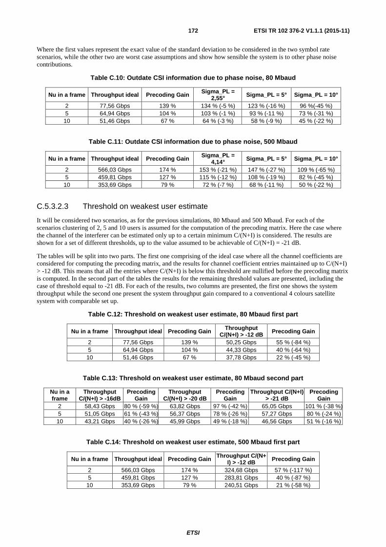
ETSI

ETSI TR 102 376-2 V1.1.1 (2015-11)172

Where the first values represent the exact value of the standard deviation to be considered in the two symbol rate scenarios, while the other two are worst case assumptions and show how sensible the system is to other phase noise contributions.

Table C.10: Outdate CSI information due to phase noise, 80 Mbaud

Nu in a frame Throughput ideal Precoding Gain Sigma_PL = 2,55° Sigma_PL = 5° Sigma_PL = 10°

2 77,56 Gbps 139 % 134 % (-5 %) 123 % (-16 %) 96 %(-45 %) 5 64,94 Gbps 104 % 103 % (-1 %) 93 % (-11 %) 73 % (-31 %)

10 51,46 Gbps 67 % 64 % (-3 %) 58 % (-9 %) 45 % (-22 %)

Table C.11: Outdate CSI information due to phase noise, 500 Mbaud

Nu in a frame Throughput ideal Precoding Gain Sigma_PL = 4,14° Sigma_PL = 5° Sigma_PL = 10°

2 566,03 Gbps 174 % 153 % (-21 %) 147 % (-27 %) 109 % (-65 %) 5 459,81 Gbps 127 % 115 % (-12 %) 108 % (-19 %) 82 % (-45 %)

10 353,69 Gbps 79 % 72 % (-7 %) 68 % (-11 %) 50 % (-22 %)

C.5.3.2.3 Threshold on weakest user estimate

It will be considered two scenarios, as for the previous simulations, 80 Mbaud and 500 Mbaud. For each of the scenarios clustering of 2, 5 and 10 users is assumed for the computation of the precoding matrix. Here the case where the channel of the interferer can be estimated only up to a certain minimum C/(N+I) is considered. The results are shown for a set of different thresholds, up to the value assumed to be achievable of C/(N+I) = -21 dB.

The tables will be split into two parts. The first one comprising of the ideal case where all the channel coefficients are considered for computing the precoding matrix, and the results for channel coefficient entries maintained up to C/(N+I) > -12 dB. This means that all the entries where C/(N+I) is below this threshold are nullified before the precoding matrix is computed. In the second part of the tables the results for the remaining threshold values are presented, including the case of threshold equal to -21 dB. For each of the results, two columns are presented, the first one shows the system throughput while the second one present the system throughput gain compared to a conventional 4 colours satellite system with comparable set up.

Table C.12: Threshold on weakest user estimate, 80 Mbaud first part

Nu in a frame Throughput ideal Precoding Gain Throughput C/(N+I) > -12 dB Precoding Gain

2 77,56 Gbps 139 % 50,25 Gbps 55 % (-84 %) 5 64,94 Gbps 104 % 44,33 Gbps 40 % (-64 %)

10 51,46 Gbps 67 % 37,78 Gbps 22 % (-45 %)

Table C.13: Threshold on weakest user estimate, 80 Mbaud second part

Nu in a frame

Throughput C/(N+I) > -16dB

Precoding Gain

Throughput C/(N+I) > -20 dB

Precoding Gain

Throughput C/(N+I) > -21 dB

Precoding Gain

2 58,43 Gbps 80 % (-59 %) 63,82 Gbps 97 % (-42 %) 65,05 Gbps 101 % (-38 %)5 51,05 Gbps 61 % (-43 %) 56,37 Gbps 78 % (-26 %) 57,27 Gbps 80 % (-24 %) 10 43,21 Gbps 40 % (-26 %) 45,99 Gbps 49 % (-18 %) 46,56 Gbps 51 % (-16 %)

Table C.14: Threshold on weakest user estimate, 500 Mbaud first part

Nu in a frame Throughput ideal Precoding Gain Throughput C/(N+I) > -12 dB Precoding Gain

2 566,03 Gbps 174 % 324,68 Gbps 57 % (-117 %) 5 459,81 Gbps 127 % 283,81 Gbps 40 % (-87 %)

10 353,69 Gbps 79 % 240,51 Gbps 21 % (-58 %)

ETSI

ETSI TR 102 376-2 V1.1.1 (2015-11)173

Table C.15: Threshold on weakest user estimate, 500 Mbaud second part

Nu in a frame

Throughput C/(N+I) > -16dB

Precoding Gain

Throughput C/(N+I) > -20 dB Precoding Gain Throughput

C/(N+I) > -21 dB Precoding Gain

2 381,65 Gbps 85 % (-89 %) 429,13 Gbps 108 % (-66%) 445,76 Gbps 116 % (-58 %) 5 330,86 Gbps 64 % (-63 %) 365,76 Gbps 80 % (-47%) 378,45 Gbps 87 % (-40 %)

10 273,74 Gbps 38 % (-41 %) 296,71 Gbps 51 % (-28%) 304,13 Gbps 54 % (-25 %)

ETSI

ETSI TR 102 376-2 V1.1.1 (2015-11)174

Annex D: Time slicing Time slicing may be applied to DVB-S2 (ETSI EN 302 307-1 [i.1]) and S2X (ETSI EN 302 307-1 [i.2]). Description of the use of time slicing can be found in annex G of ETSI TR 102 376-1 [i.3].

ETSI

ETSI TR 102 376-2 V1.1.1 (2015-11)175

Annex E: IMUX and OMUX filters characteristics The attachment tr_10237602v010101p0.zip gives the amplitude and group delay numerical entries for the IMUX and OMUX filters described in clause 4.4.1.2, for 26 MHz, 33 MHz and 36 MHz transponder bandwidth.

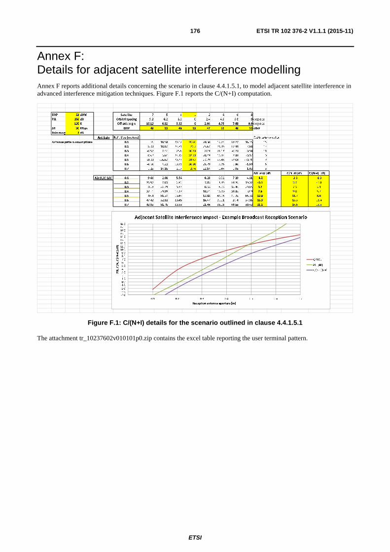
ETSI

ETSI TR 102 376-2 V1.1.1 (2015-11)176

Annex F: Details for adjacent satellite interference modelling Annex F reports additional details concerning the scenario in clause 4.4.1.5.1, to model adjacent satellite interference in advanced interference mitigation techniques. Figure F.1 reports the C/(N+I) computation.

Figure F.1: C/(N+I) details for the scenario outlined in clause 4.4.1.5.1

The attachment tr_10237602v010101p0.zip contains the excel table reporting the user terminal pattern.

EIRP 53 dBW Satellite 7 5 3 1 2 4 6 8

FSL 206 dB Orbital spacing -9.2 -6.2 -3.2 0 2.4 4.3 6.8 9 degrees

120 K Off axis angle -10.12 -6.82 -3.52 0 2.64 4.73 7.48 9.9 degrees

SR 30 MSps EIRP 48 53 48 53 47 53 48 53 dBW

Rain marg 3 dB

Ant Gain Refl. Size [meters] Table column index

Antenna pattern assumptions 0.1 16 18.58 20.12 20.66 20.38 19.74 18.27 16.35 15

0.2 5.73 18.87 24.81 26.7 25.67 23.35 17.44 7.68 13

0.3 -0.57 7.44 25.8 30.23 27.9 22.17 -0.23 0.58 11

0.4 0.62 3.64 24.36 32.73 28.49 16.34 2.88 -0.17 9

0.5 -8.73 -26.67 20.23 34.67 27.79 -7.48 -2.08 -30.71 7

0.6 -6.16 4.23 10.81 36.26 25.79 7.25 1.86 -1.69 5

0.7 -1.35 -14.15 2.97 37.6 22.14 1.44 -1.95 -1.83 3

ASI_aggr [dB] C/N_dl [dB] C/(N+I) [dB]

ASI (C/I) [dB] 0.1 9.66 2.08 5.54 6.28 0.92 7.39 4.31 -4.2 -2.3 -6.3

0.2 25.97 7.83 6.89 7.03 3.35 14.26 19.02 -0.3 3.7 -1.8

0.3 35.8 22.79 9.43 8.33 8.06 35.46 29.65 3.7 7.3 2.1

0.4 37.11 29.09 13.37 10.24 16.39 34.85 32.9 7.8 9.8 5.7

0.5 48.4 61.34 19.44 12.88 42.15 41.75 65.38 12.0 11.7 8.8

0.6 47.42 32.03 30.45 16.47 29.01 39.4 37.95 15.9 13.3 11.4

0.7 43.95 51.75 39.63 21.46 36.16 44.55 39.43 21.1 14.6 13.8

-4.0

-3.0

-2.0

-1.0

0.0

1.0

2.0

3.0

4.0

5.0

6.0

7.0

8.0

9.0

10.0

11.0

12.0

13.0

14.0

15.0

16.0

17.0

18.0

0 0.1 0.2 0.3 0.4 0.5 0.6 0.7

ASI, C/N, C/(N+I) [dB]

Reception antenna aperture [m]

Adjacent Satellite Interference Impact - Example Broadcast Reception Scenario

C/N DL

ASI [dB]

C/(N+I) [dB]

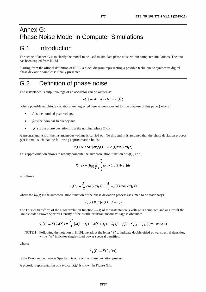
ETSI

ETSI TR 102 376-2 V1.1.1 (2015-11)177

Annex G: Phase Noise Model in Computer Simulations

G.1 Introduction The scope of annex G is to clarify the model to be used to simulate phase noise within computer simulations. The text has been copied from [i.18].

Starting from the official definition of IEEE, a block diagram representing a possible technique to synthesize digital phase deviation samples is finally presented.

G.2 Definition of phase noise The instantaneous output voltage of an oscillator can be written as:

���� = ����(2���� + ����) (where possible amplitude variations are neglected here as non-relevant for the purpose of this paper) where:

• A is the nominal peak voltage,

• f0 is the nominal frequency and

• ϕ(t) is the phase deviation from the nominal phase 2 πf0 t

A spectral analysis of the instantaneous voltage is carried out. To this end, it is assumed that the phase deviation process ϕ(t) is small such that the following approximation holds:

���� ≈ �����2����� − �����sin(2����) This approximation allows to readily compute the autocorrelation function of v(t) , i.e.:

����� ≡ lim�→�

1�� �{��

���

������� + ��}�� as follows:

����� = ��

2cos�2����� + ��

2����� cos�2�����

where the Rϕ(τ) is the autocorrelation function of the phase deviation process (assumed to be stationary):

����� ≡ �{������� + ��} The Fourier transform of the autocorrelation function Rv(τ) of the instantaneous voltage is computed and as a result the Double-sided Power Spectral Density of the oscillator instantaneous voltage is obtained:

���� ≡ !"�����# = ��4$%�� − ��� + %�� + ��� + ��� − ��� + ��� + ���&(���'���1)

NOTE 1: Following the notation in [i.16], we adopt the letter "S" to indicate double-sided power spectral densities, while "W" indicates single-sided power spectral densities.

where:

�(�) ≡ !{�����} is the Double-sided Power Spectral Density of the phase deviation process.

A pictorial representation of a typical Sv(f) is shown in Figure G.1.

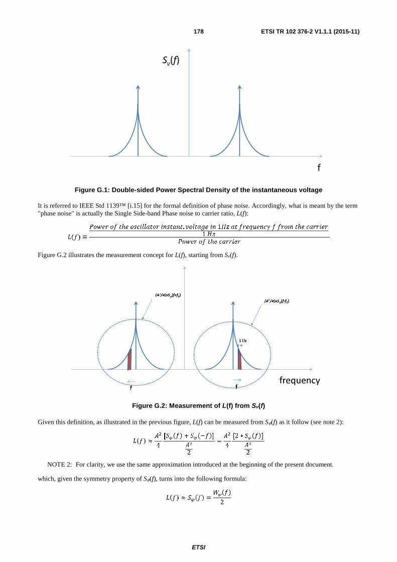
ETSI

ETSI TR 102 376-2 V1.1.1 (2015-11)178

Figure G.1: Double-sided Power Spectral Density of the instantaneous voltage

It is referred to IEEE Std 1139™ [i.15] for the formal definition of phase noise. Accordingly, what is meant by the term "phase noise" is actually the Single Side-band Phase noise to carrier ratio, L(f):

((�) ≡ ��)�*���ℎ����+,,-��*+'��-'�. ��,�-.�+'1/0-��*�12�'�3��*�4�ℎ��-**+�*1/0 ��)�*���ℎ��-**+�*

Figure G.2 illustrates the measurement concept for L(f), starting from Sv(f).

Figure G.2: Measurement of L(f) from Sv(f)

Given this definition, as illustrated in the previous figure, L(f) can be measured from Sϕ(f) as it follow (see note 2):

(��� ≈ ��

4

[ ���� + ��−��]��2

=��

4

[2 ∗ ����]��

2

NOTE 2: For clarity, we use the same approximation introduced at the beginning of the present document.

which, given the symmetry property of Sϕ(f), turns into the following formula:

(��� ≈ ���� = 5����2

f

Sv(f)

frequencyf

1 Hz

f

(A2/4)xSϕ(f-f0)

(A2/4)xSϕ(f+f0)

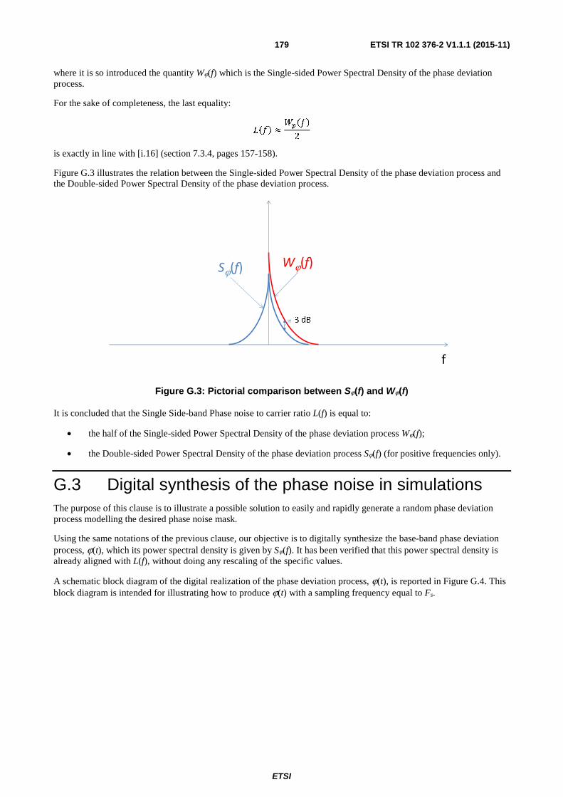
ETSI

ETSI TR 102 376-2 V1.1.1 (2015-11)179

where it is so introduced the quantity Wϕ(f) which is the Single-sided Power Spectral Density of the phase deviation process.

For the sake of completeness, the last equality:

���� ≈�����

2

is exactly in line with [i.16] (section 7.3.4, pages 157-158).

Figure G.3 illustrates the relation between the Single-sided Power Spectral Density of the phase deviation process and the Double-sided Power Spectral Density of the phase deviation process.

Figure G.3: Pictorial comparison between Sϕ(f) and Wϕ(f)

It is concluded that the Single Side-band Phase noise to carrier ratio L(f) is equal to:

• the half of the Single-sided Power Spectral Density of the phase deviation process Wϕ(f);

• the Double-sided Power Spectral Density of the phase deviation process Sϕ(f) (for positive frequencies only).

G.3 Digital synthesis of the phase noise in simulations The purpose of this clause is to illustrate a possible solution to easily and rapidly generate a random phase deviation process modelling the desired phase noise mask.

Using the same notations of the previous clause, our objective is to digitally synthesize the base-band phase deviation process, ϕ(t), which its power spectral density is given by Sϕ(f). It has been verified that this power spectral density is already aligned with L(f), without doing any rescaling of the specific values.

A schematic block diagram of the digital realization of the phase deviation process, ϕ(t), is reported in Figure G.4. This block diagram is intended for illustrating how to produce ϕ(t) with a sampling frequency equal to Fs.

f

Sϕ(f)Wϕ(f)

3 dB

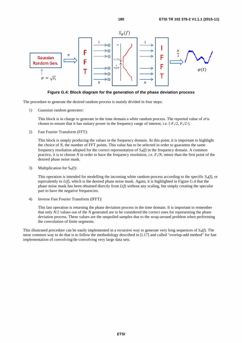
ETSI

ETSI TR 102 376-2 V1.1.1 (2015-11)180

Figure G.4: Block diagram for the generation of the phase deviation process

The procedure to generate the desired random process is mainly divided in four steps:

1) Gaussian random generator:

This block is in charge to generate in the time domain a white random process. The reported value of σ is chosen to ensure that it has unitary power in the frequency range of interest, i.e. [-Fs/2, Fs/2-].

2) Fast Fourier Transform (FFT):

This block is simply producing the values in the frequency domain. At this point, it is important to highlight the choice of N, the number of FFT points. This value has to be selected in order to guarantee the same frequency resolution adopted for the correct representation of Sϕ(f) in the frequency domain. A common practice, it is to choose N in order to have the frequency resolution, i.e. Fs/N, minor than the first point of the desired phase noise mask.

3) Multiplication for Sϕ(f):

This operation is intended for modelling the incoming white random process according to the specific Sϕ(f), or equivalently to L(f), which is the desired phase noise mask. Again, it is highlighted in Figure G.4 that the phase noise mask has been obtained directly from L(f) without any scaling, but simply creating the specular part to have the negative frequencies.

4) Inverse Fast Fourier Transform (IFFT):

This last operation is returning the phase deviation process in the time domain. It is important to remember that only N/2 values out of the N generated are to be considered the correct ones for representing the phase deviation process. These values are the unspoiled samples due to the wrap-around problem when performing the convolution of finite segments.

This illustrated procedure can be easily implemented in a recursive way to generate very long sequences of Sϕ(f). The most common way to do that is to follow the methodology described in [i.17] and called "overlap-add method" for fast implementation of convolving/de-convolving very large data sets.

ETSI

ETSI TR 102 376-2 V1.1.1 (2015-11)181

Annex H: Bibliography S. Scalise, H. Ernst, G. Harles: "Measurement and Modeling of the Land Mobile Satellite Channel at Ku-Band", IEEE Transactions on Vehicular Technology, volume 57, number 2, March 2008.

ETSI

ETSI TR 102 376-2 V1.1.1 (2015-11)182

History

Document history

V1.1.1 February 2005 Publication as ETSI TR 102 376

V1.1.1 November 2015 Publication