TPRS A 147843 1. - dep.ufscar.br proofs.pdf · AUTHOR QUERIES Journal id: TPRS_A_147843...

AUTHOR QUERIES Journal id: TPRS_A_147843 Corresponding author: H. H. YANASSE Title: Linear models for 1-group two-dimensional guillotine cutting problems

Query number Query

1 Please supply “Received” and “in final form” dates 2 Please supply page range 3 Please supply place of publication 4 Please supply the date website accessed

New XML Template (2005) [4.2.2006–4:55pm] [1–21]{TandF}TPRS/TPRS_A_147843.3d (TPRS) TPRS_A_147843

International Journal of Production Research,Vol. ??, No. ?, Month?? 2006, 1–21

Linear models for 1-group two-dimensional

guillotine cutting problems

H. H. YANASSE*y and R. MORABITOz

yLaboratorio Associado de Computacao e Matematica Aplicada,

Instituto Nacional de Pesquisas Espaciais, 12227-010 – Sao Jose dos Campos – SP, Brazil

zDepartamento de Engenharia de Producao, Universidade Federal de Sao Carlos,

13565-905 – Sao Carlos – SP, Brazil

(Received 2222; in final form 2222)

In this study we present integer linear and non-linear models to generate 1-groupconstrained and unconstrained two-dimensional guillotine cutting patterns,including exact and non-exact cases. These patterns appear in different cuttingprocesses as, for example, in the furniture industry. The models are usefulfor research and development of more effective solution methods, exploringparticular structures, model decomposition, model relaxations, etc. They are alsohelpful for the performance evaluation of heuristic methods, since they allow(at least for problems of moderate size) an estimation of the optimality gapof heuristic solutions. To demonstrate the effectiveness of the proposed models,we compare them with models of the literature by solving a number of examplesrandomly generated and an actual example derived from a furniture company.Such results were produced using a well-known commercial software (themodelling language GAMS and the solver CPLEX) and they show that thecomputational efforts required to solve the models can be very different.

Keywords: Cutting and packing problems; 1-group guillotine cutting; Integerlinear models; Furniture industry

1. Introduction

Cutting problems are found in many industrial processes where paper and

aluminium rolls, glass and fibreglass plates, metal bars and sheets, hardboards,pieces of leather and cloth, etc., are cut in order to produce smaller pieces of ordered

sizes and quantities. The problem is to determine the ‘best’ way of cutting largeobjects to produce the ordered items so that an objective is optimised, for example,

with minimum trim loss. For surveys and special issues on cutting and packingproblems and their industrial applications, readers may consult Dyckhoff and

Waescher (1990), Lirov (1992), Dowsland and Dowsland (1992), Sweeney andPaternoster (1992), Dyckhoff and Finke (1992), Martello (1994a, 1994b), Bischoff

and Waescher (1995), Mukhacheva (1997), Dyckhoff et al. (1997), Arenales et al.(1999), Wang and Waescher (2002), Hifi (2002), Lodi et al. (2002) and SICUP (2004).

*Corresponding author. Email: [email protected]

International Journal of Production Research

ISSN 0020–7543 print/ISSN 1366–588X online � 2006 Taylor & Francis

http://www.tandf.co.uk/journals

DOI: 10.1080/00207540500478603

1

2

3

4

5

6

7

8

9

10

11

12

13

14

15

16

17

18

19

20

21

22

23

24

25

26

27

28

29

30

31

32

33

34

35

36

37

38

39

40

41

42

43

44

45

46

47

48

proofreader

Text Box

1


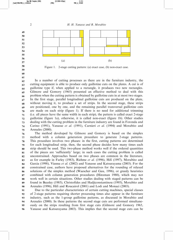
In a number of cutting processes as there are in the furniture industry, thecutting equipment is able to produce only guillotine cuts on the plates. A cut is ofguillotine type if, when applied to a rectangle, it produces two new rectangles.Gilmore and Gomory (1965) presented an effective method to deal with thisproblem when the cutting pattern is obtained by guillotine cuts in at most two stages.In the first stage, parallel longitudinal guillotine cuts are produced on the plate,without moving it, to produce a set of strips. In the second stage, these stripsare positioned, one by one, and the remaining parallel transversal guillotine cutsare made on each strip (figure 1). If there is no need for additional trimming(i.e. all pieces have the same width in each strip), the pattern is called exact 2-stageguillotine (figure 1a), otherwise, it is called non-exact (figure 1b). Other studiesdealing with the cutting problem in the furniture industry are found in Foronda andCarino (1991), Yanasse et al. (1991), Carnieri et al. (1994) and Morabito andArenales (2000).

The method developed by Gilmore and Gomory is based on the simplexmethod with a column generation procedure to generate 2-stage patterns.This procedure involves two phases: in the first, cutting patterns are determinedfor each longitudinal strip, then, the second phase decides how many times eachstrip should be used. This two-phase method works well if the ordered quantitiesof the pieces are ‘sufficiently’ large; in such cases the cutting problem is calledunconstrained. Approaches based on two phases are common in the literature,as for example in Farley (1983), Riehme et al. (1996), Hifi (1997), Morabito andGarcia (1998), Vianna et al. (2002) and Yanasse and Katsurayama (2003). For theconstrained case, authors have proposed alternatives for the rounding of relaxedsolutions of the simplex method (Waescher and Gau, 1996), or greedy heuristicscombined with column generation procedures (Hinxman 1980), which may notwork well in certain situations. Other studies dealing with staged patterns can befound in Beasley (1985), Christofides and Hadjiconstantinou (1995), Morabito andArenales (1996), Hifi and Roucairol (2001) and Lodi and Monaci (2003).

Due to the particular characteristics of certain cutting machines, special classesof 2-stage patterns requiring shorter processing times also appear in the furnitureindustry, such as the 1-group guillotine patterns, as discussed in Morabito andArenales (2000). In these patterns the second stage cuts are performed simultane-ously on the strips resulting from first stage cuts (Gilmore and Gomory 1965,Yanasse and Katsurayama 2003). This implies that the second stage cuts can be

(a) (b)

Figure 1. 2-stage cutting pattern: (a) exact case, (b) non-exact case.

2 H. H. Yanasse and R. Morabito

49

50

51

52

53

54

55

56

57

58

59

60

61

62

63

64

65

66

67

68

69

70

71

72

73

74

75

76

77

78

79

80

81

82

83

84

85

86

87

88

89

90

91

92

93

94

95

96


produced together with the first stage cuts, without moving the strips and, in thisway, save processing time. Gilmore and Gomory (1965) also discussed p-grouppatterns, p>1. The 1-group patterns can be non-homogeneous (a pattern ishomogeneous if it contains only pieces of the same type), and exact and non-exact depending on the need for additional trimming, as illustrated in figure 2(note in the exact patterns that there is no need for additional trimming, since allpieces have the same width in each horizontal strip and all pieces have the samelength in each vertical strip).

A few studies were found in the literature presenting mathematical program-ming formulations for 1-group two-dimensional guillotine cutting problems(Morabito and Arenales 2000, Scheithauer 2002). Models for such problems areuseful for research and development of more effective solution methods, exploringspecial features and particular structures, model decomposition, model relaxations,etc. These models are also helpful for the performance evaluation of heuristicmethods, since they allow (at least for problems of moderate size) an estimationof the optimality gap of heuristic solutions. Thus motivated by this, the presentstudy proposes new integer linear and non-linear models to generate 1-group cuttingpatterns, including exact and non-exact cases, and constrained and unconstrainedcases. It is worth mentioning that we are not aware of exact algorithms forsuch problems in the literature. The only exception is the work by Yanasse andKatsurayama (2003), where an enumeration algorithm is proposed for the specialcase of exact and unconstrained 1-group two-dimensional guillotine cutting pattern.In theory, such algorithm could be extended to cover non-exact and constrainedcases by enumerating all possible combinations of strips and rejecting those solutionsthat do not satisfy the constraints. This procedure, however, is ineffective andtime consuming; hence, it was discarded by those authors. The 1-group models canbe used in the column generation procedure of Gilmore and Gomory’s approach,

(a)

(b)

(c)

(d)

Figure 2. 1-group cutting pattern: (a) and (b) exact cases, (c) and (d) non-exact cases.

Linear models for 1-group 2D guillotine cutting problems 3

97

98

99

100

101

102

103

104

105

106

107

108

109

110

111

112

113

114

115

116

117

118

119

120

121

122

123

124

125

126

127

128

129

130

131

132

133

134

135

136

137

138

139

140

141

142

143

144


or combined with repeated exhausted reduction heuristics (Hinxman 1980), to solvecutting stock problems.

This paper is organised as follows. In section 2 we review existing models andpropose new models for 1-group cutting problems. In section 3, to demonstrate theeffectiveness of the proposed models, we compare them with models of the litera-ture by solving a number of examples randomly generated and an actual examplederived from a furniture company. We chose to use the well-known commercialsoftware modelling language GAMS and the mixed integer linear programmingsolver CPLEX (Brooke et al. 1992). The results show that the computational effortsrequired to solve the models can be very different. Finally, in section 4 we presentconcluding remarks and discuss perspectives for future research.

2. 1-group cutting models

Without loss of generality, the models below assume that the orientation of thepieces is fixed, that is, the pieces cannot rotate. Consider the following parameters:

L, W length and width of the plateli, wi length and width of piece type i (i¼ 1, . . . ,m)

lmin, wmin minimum length and minimum width, respectively, of the pieceslmax, wmax maximum length and maximum width, respectively, of the pieces

vi, bi value (e.g. area) and demand of piece type i

2.1 Non-linear model

Initially we present an integer non-linear model for the non-exact case. Let:

J, K number of different lengths li and widths wi, respectively.vijk¼ vi, if li� lj and wi�wk

0, otherwise.

Variables:

�j number of times length lj is cut along L�k number of times width wk is cut along Waijk number of rectangles lj�wk containing a piece of type i (i.e. number

of type i pieces contained in all rectangles lj�wk)

maxXm

i¼1

XJ

j¼1

XK

k¼1

vijkaijk ð1Þ

XJ

j¼1

lj�j � L ð2Þ


145

146

147

148

149

150

151

152

153

154

155

156

157

158

159

160

161

162

163

164

165

166

167

168

169

170

171

172

173

174

175

176

177

178

179

180

181

182

183

184

185

186

187

188

189

190

191

192


XK

k¼1

wk�k �W ð3Þ

Xm

i¼1

aijk � �j�k, for all j, k ð4Þ

XJ

j¼1

XK

k¼1

aijk � bi, for all i ð5Þ

with

�j,�k, aijk � 0, integer, i ¼ 1, . . . , m; j ¼ 1, . . . , J; k ¼ 1, . . . , K: ð6Þ

Note that �j�k corresponds to the number of rectangles lj�wk inthe pattern. The objective function (1) maximises the total value of the piecescut in the pattern, constraints (2) and (3) guarantee that the piece lengths and widthsdo not exceed the plate length and width, respectively, constraints (4) limit thevariables aijk to �j�k, constraints (5) refer to the availability of the pieces andconstraints (6) refer to the non-negativity and integrity of the variables.

Model (1)–(6) can be adapted to deal with the exact case by simply redefiningvijk as:

vijk ¼vi, if li ¼ lj and wi ¼ wk for any i ¼ 1, . . . ,m

0, otherwise:

In this case, if two piece types i1 and i2 have the same size (li1, wi1)¼(li2, wi2)¼ (lj, wk) and the same value vi1¼ vi2¼ vjk (e.g. the area of rectangle lj�wk),we can also reduce the number of model variables by defining ajk ¼

Pmi¼1 aijk, the

number of rectangles lj�wk containing a piece lj�wk (i.e. the number of pieceslj�wk). Model (1)–(6) reduces to:

maxXJ

j¼1

XK

k¼1

vjkajk ð7Þ

XJ

j¼1

lj�j � L ð8Þ

XK

k¼1

wk�k �W ð9Þ

ajk � �j�k, for all j, k ð10Þ

ajk � bi if li ¼ lj, wi ¼ wk for any i ¼ 1, . . . , m; for all j, k ð11Þ

with

�j, �k, ajk � 0, integer, j ¼ 1, . . . , J; k ¼ 1, . . . ,K: ð12Þ


193

194

195

196

197

198

199

200

201

202

203

204

205

206

207

208

209

210

211

212

213

214

215

216

217

218

219

220

221

222

223

224

225

226

227

228

229

230

231

232

233

234

235

236

237

238

239

240


If the problem is unconstrained, we can eliminate constraint (10) and (11) of

model (7)–(12), and replace the variables ajk¼ �j�k, obtain the integer quadratic

model in Morabito and Arenales (2000):

maxXJ

j¼1

XK

k¼1

vjk�j�k

XJ

j¼1

lj�j � L

XK

k¼1

wk�k �W

with

�j, �k � 0, integer, j ¼ 1, . . . , J; k ¼ 1, . . . ,K:

To adapt this model for the non-exact case, it is enough to redefine:

vjk ¼ maxi¼1,...,m

vijli � lj,wi � wk

� �

Moreover, if rectangle lj�wk can contain more than one piece, vjk is redefined

as the value of the best homogeneous solution:

vjk ¼ maxi¼1,...,m

vi lj=li� �

wk=wi

� ��

2.2 Linear model 1

These non-linear models can be linearised in the following way (Harjunkoski et al.

1997): consider for instance model (1)–(6) and let �j ¼Psj

s¼1 2s�1�js, where �js2 {0, 1}

and sj is so that: 2sj�1 � L=lj� �

< 2sj , that is, sj is the maximum number of bits for

a binary representation of �j (the same could be done choosing �k instead of �j).The non-linear constraint (4) is rewritten as:

Xm

i¼1

aijk �Xsj

s¼1

2s�1�js�k, for all j, k

which can be replaced by the following set of linear constraints:

Xm

i¼1

aijk �Xsj

s¼1

2s�1fjks, for all j, k

fjks � �k, for all j, k, s

fjks � �k �Mð1� �jsÞ, for all j, k, s


241

242

243

244

245

246

247

248

249

250

251

252

253

254

255

256

257

258

259

260

261

262

263

264

265

266

267

268

269

270

271

272

273

274

275

276

277

278

279

280

281

282

283

284

285

286

287

288


fjks �M�js, for all j, k, s

�js 2 f0,1g, for all j, s

where M is a sufficiently large number (e.g. W=wmin

� �). Note that if �js¼ 1 then

fjks¼�k, on the other hand, if �js¼ 0 then fjks¼ 0. Model (1)–(6) is rewritten as:

Model 1:

maxXm

i¼1

XJ

j¼1

XK

k¼1

vijkaijk ð13Þ

XJ

j¼1

ljXsj

s¼1

2s�1�js � L ð14Þ

XK

k¼1

wk�k �W ð15Þ

Xm

i¼1

aijk �Xsj

s¼1

2s�1fjks, for all j, k ð16Þ

fjks � �k, for all j, k, s ð17Þ

fjks � �k �Mð1� �jsÞ, for all j, k, s ð18Þ

fjks �M�js, for all j, k, s ð19Þ

XJ

j¼1

XK

k¼1

aijk � bi, for all i ð20Þ

with

�js 2 f0,1g, �k, aijk � 0, integer, fjks � 0, i ¼ 1, . . . , m; j ¼ 1, . . . , J;

k ¼ 1, . . . , K, s ¼ 1, . . . , sjð21Þ

Similarly to the integer non-linear model (1)–(6), the exact case can also be treated

by model 1 simply redefining vijk by:

vijk ¼ vi, if li ¼ lj and wi ¼ wk for any i ¼ 1, . . . , m

0, otherwise:

(or redefining vijk and aijk by vjk and ajk, respectively, as discussed above, to reduce

the number of variables).


289

290

291

292

293

294

295

296

297

298

299

300

301

302

303

304

305

306

307

308

309

310

311

312

313

314

315

316

317

318

319

320

321

322

323

324

325

326

327

328

329

330

331

332

333

334

335

336


2.3 Linear model 2

Scheithauer (2002) presented an integer linear model for the non-exact 1-group

problem. For convenience, we present below Scheithauer’s model here called

model 2. Let:

P, Q maximum number of strips from left to right and from bottom to top,

respectively, in the pattern (P¼ L=lmin

� �, Q¼ W=wmin

� �)

Variables:

Lj length of the jth strip (left to right) in the pattern ( j¼ 1, . . . ,P)Wk width of the kth strip (bottom to top) in the pattern (k¼ 1, . . . ,Q)

xijk¼ 1, if a type i piece is placed in rectangle Lj�Wk

0, otherwise.

Model 2:

maxXm

i¼1

XP

j¼1

XQ

k¼1

vixijk ð22Þ

XP

j¼1

Lj � L ð23Þ

XQ

k¼1

Wk �W ð24Þ

Xm

i¼1

xijk � 1, for all j, k ð25Þ

Xm

i¼1

lixijk � Lj, for all j, k ð26Þ

Xm

i¼1

wixijk �Wk, for all j, k ð27Þ

XP

j¼1

XQ

k¼1

xijk � bi, for all i ð28Þ

Lj � Ljþ1, for all j ð29Þ

Wk �Wkþ1, for all k ð30Þ


337

338

339

340

341

342

343

344

345

346

347

348

349

350

351

352

353

354

355

356

357

358

359

360

361

362

363

364

365

366

367

368

369

370

371

372

373

374

375

376

377

378

379

380

381

382

383

384


with

xijk 2 f0,1g, Lj, Wk � 0, i ¼ 1, . . . , m; j ¼ 1, . . . , P; k ¼ 1, . . . , Q: ð31Þ

The objective function (22) maximises the total value of the pieces cut in thepattern. Constraints (23) and (24) guarantee that the lengths and widths of the stripsarranged in the pattern do not exceed the plate length and width, respectively.Constraints (25) impose that at most one piece is placed in each rectangle Lj�Wk.Constraints (26) and (27) guarantee that the piece lengths and widths in eachrectangle Lj�Wk, do not exceed the rectangle length and width, respectively.Constraints (28) refer to the availability of pieces and constraints (31) refer to thenon-negativity and integrality of the variables. Note that constraints (29) and (30)are included to eliminate symmetries (and reduce the solution space). Note alsoin (31) that the variables Lj and Wk need not to be integer.

Model (22)–(31) can also be adapted to deal with the exact case. For this, ina first impulse, one might think that it would be sufficient replacing inequalities (26)and (27) by the equalities:

Xm

i¼1

lixijk ¼ Lj, for all j, k ð32Þ

Xm

i¼1

wixijk ¼Wk, for all j, k ð33Þ

However, these constraints are valid only for the case where there is some pieceof type i placed in rectangle Lj�Wk. If there is no piece in such rectangle,these constraints need not to be satisfied. To impose constraint (32) only for thiscase, we add the following constraints:

Xm

i¼1

lixijk � Lj, for all j, k ð34Þ

Lj �Xm

i¼1

lixijk þM 1�Xm

i¼1

xijk

!, for all j, k ð35Þ

where M is a sufficiently large number (e.g. M¼ lmax). Similarly, to imposeconstraint (33) only when there is some piece of type i placed in rectangle Lj�Wk,we add constraints:

Xm

i¼1

wixijk �Wk, for all j, k ð36Þ

Wk �Xm

i¼1

wixijk þM 1�Xm

i¼1

xijk

!, for all j, k ð37Þ

where M is a sufficiently large number (e.g. M¼wmax). This way, the 1-group modelfor the exact case is obtained simply replacing in model 2 (formulation (22)–(31))constraints (26) and (27) by constraints (34)–(37).


385

386

387

388

389

390

391

392

393

394

395

396

397

398

399

400

401

402

403

404

405

406

407

408

409

410

411

412

413

414

415

416

417

418

419

420

421

422

423

424

425

426

427

428

429

430

431

432


In table 1 models 1 and 2 (1-group cutting) are compared in terms of thenumber of variables and constraints for the non-exact case. For the exact casewe have the same number of variables and constraints, except that in model 2we have 2PQ additional constraints.

2.4 Other linear models

Vianna et al. (2002) presented an integer non-linear model for the non-exact 2-stagetwo-dimensional guillotine cutting problem, which can be linearised using the sameprocedure of section 2.1. Lodi and Monaci (2003) presented other two interestinginteger linear models for the 2-stage case, based on the restriction of packing(cutting) the pieces into shelves (i.e. rows forming levels). A shelf is a slice of theplate with length L and width coincident with the width of the widest piece cut offfrom it. Their observation is that each feasible solution of (such two-dimensionalpacking) with trimming is composed of shelves, and, vice-versa, each itempacked into a shelf can be cut off in at most two stages (plus trimming). It isworth mentioning that these models’ formulations cannot be extended (at leastin a straightforward manner) to the 1-group case, since there are difficulties inenforcing the constraint that the second stage cuts should be all in the samepositions, for all the strips.

3. Computational experiments

For the sake of illustration, in this section we present the computational resultsobtained by applying models 1 and 2 for some 1-group examples. The modelswere codified in the modelling language GAMS (Brooke et al. 1992) and solvedby the integer linear programming solver CPLEX (version 7) in a microcomputerPentium IV with 2.8GHz, 512Mb RAM. We use the standard default settingsof CPLEX, that is, we did not explore problem-oriented branching rules, initialheuristic solutions, problem-specific valid inequalities, etc. In the first set of examplesthe values of the pieces are equal to their respective areas (i.e. vi¼ liwi); this way,a simple upper bound equal to the plate area LW may be imposed on their models.The solution values presented in the tables below are in percentage of the plate areautilisation. In all the tests performed, the exact and non-exact results were obtainedusing the same problem by solving models 1 and 2 with the indicated alternativeconstraints as described in section 2.

Table 2 presents the input data of a simple constrained two-dimensionalguillotine cutting problem analysed in Vianna et al. (2002). We assume that the

Table 1. Comparison of the number of variables and constraints of models 1 and 2.

Number of variables Number of constraints

Model 1 mJKþ ðKþ 1ÞPJ

j¼1

1þ log L=lj� ��

þ K 2þ JKþ 3KPJ

j¼1

1þ log L=lj� ��

þm

Model 2 PþQþmPQ 2þ 3PQþPþQþm


433

434

435

436

437

438

439

440

441

442

443

444

445

446

447

448

449

450

451

452

453

454

455

456

457

458

459

460

461

462

463

464

465

466

467

468

469

470

471

472

473

474

475

476

477

478

479

480


orientation of the pieces is fixed, that is, the pieces cannot rotate. Table 3 presentsthe results obtained by models 1 and 2 with GAMS/CPLEX for such example.The 1-group optimal solutions were found in relatively small computer runtimes.We observe that the linear programming relaxation of the model (row LP relax)provides a quite loose upper bound for the problem. The gap between theLP relaxation and the final solution is over 100%. The LP relaxation value ofmodel 1 is tighter than the one of model 2 for the exact case, but it is larger forthe non-exact case. This result is observed in most of the experiments below.

Also, we can notice a difference in execution times when we impose the knownupper bound of 10 000 (i.e. the area LW of the plate) on the optimal value of theproblem (row UB¼LW), compared with the case where we do not set any bound(row No UB). It can be observed that the execution times were, in general, shorterwhen we do not impose any upper bound. These differences in model performanceand the large gap between the LP relaxation and the final solution are observedin other examples, as shown in the following computational text results.

We randomly generated constrained examples with plate (L,W)¼ (100, 100)and m¼ 5, 10, 20, 50 and 100 piece types (li,wi) sampled from uniform distributionsin the intervals [0.1L, 0.5L] and [0.1W, 0.5W], respectively (after being sampled, liand wi were simply rounded). The quantities bi were also sampled (and then rounded)from uniform distributions in the intervals [1, L=li

� �W=wi

� �]. For each value

of the parameter m, 10 instances were considered. We assume that the orientationof the pieces is fixed, that is, the pieces cannot rotate. We imposed a time limit of180 seconds for the computer runtime of each problem instance.

In table 4 the results obtained by models 1 and 2 with m¼ 5 are presented,considering the exact case. On average, the LP relaxation value of model 1 is tighterthan the one of model 2. Note that model 1 maintains its superior performance with

Table 2. Constrained example in Vianna et al. (2002) with(L, W)¼ (100, 100).

Pieces i li wi bi

1 33 14 82 20 38 43 15 43 44 40 43 35 31 44 3

Table 3. Results of models 1 and 2 (1-group patterns) for the example in Vianna et al. (2002).

Non-exact case Exact case

Example Model 1 Model 2 Model 1 Model 2

LP relax 185.68 171.13 142.73 171.13Solution 83.64 83.64 64.50 64.50Time (UB¼LW) (s) 0.5 1.0 0.1 1.2Time (No UB) (s) 0.3 0.6 0.1 0.5


481

482

483

484

485

486

487

488

489

490

491

492

493

494

495

496

497

498

499

500

501

502

503

504

505

506

507

508

509

510

511

512

513

514

515

516

517

518

519

520

521

522

523

524

525

526

527

528


respect to model 2 in terms of runtime. Note also that the average runtime issmaller when we do not impose an upper bound (columns No UB).

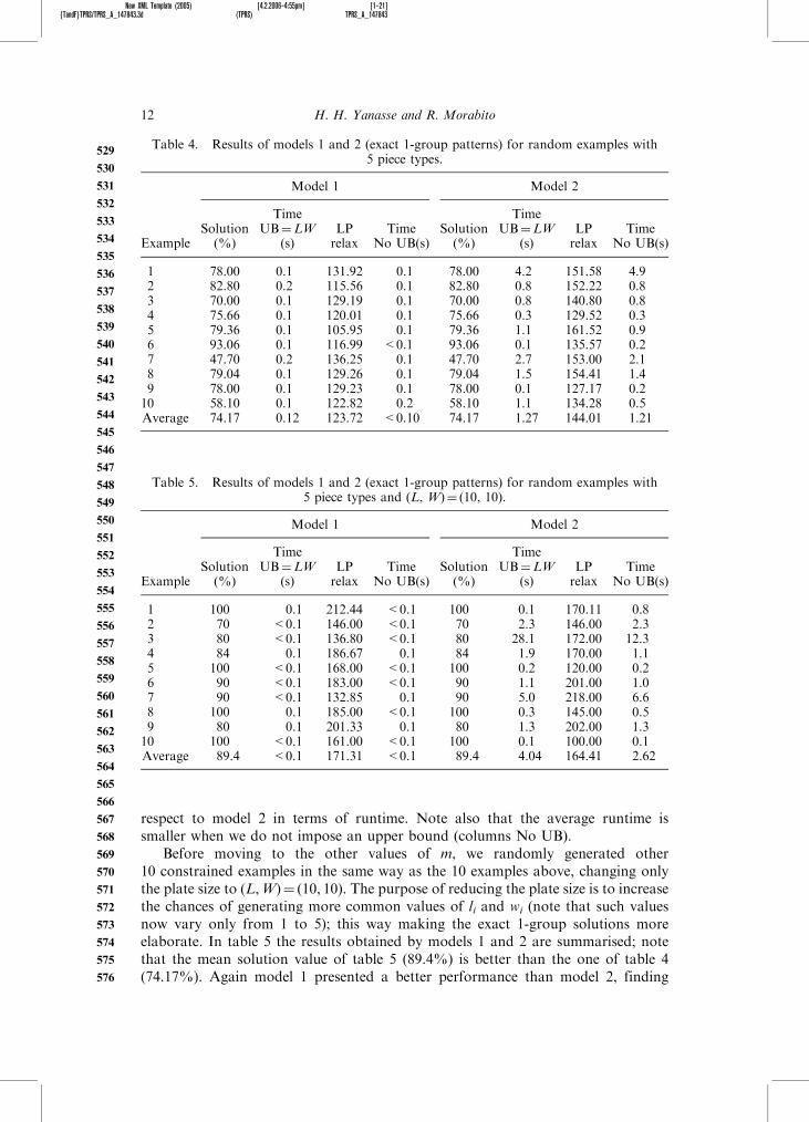
Before moving to the other values of m, we randomly generated other10 constrained examples in the same way as the 10 examples above, changing onlythe plate size to (L,W)¼ (10, 10). The purpose of reducing the plate size is to increasethe chances of generating more common values of li and wi (note that such valuesnow vary only from 1 to 5); this way making the exact 1-group solutions moreelaborate. In table 5 the results obtained by models 1 and 2 are summarised; notethat the mean solution value of table 5 (89.4%) is better than the one of table 4(74.17%). Again model 1 presented a better performance than model 2, finding

Table 4. Results of models 1 and 2 (exact 1-group patterns) for random examples with5 piece types.

Model 1 Model 2

ExampleSolution(%)

TimeUB¼LW

(s)LPrelax

TimeNo UB(s)

Solution(%)

TimeUB¼LW

(s)LPrelax

TimeNo UB(s)

1 78.00 0.1 131.92 0.1 78.00 4.2 151.58 4.92 82.80 0.2 115.56 0.1 82.80 0.8 152.22 0.83 70.00 0.1 129.19 0.1 70.00 0.8 140.80 0.84 75.66 0.1 120.01 0.1 75.66 0.3 129.52 0.35 79.36 0.1 105.95 0.1 79.36 1.1 161.52 0.96 93.06 0.1 116.99 <0.1 93.06 0.1 135.57 0.27 47.70 0.2 136.25 0.1 47.70 2.7 153.00 2.18 79.04 0.1 129.26 0.1 79.04 1.5 154.41 1.49 78.00 0.1 129.23 0.1 78.00 0.1 127.17 0.210 58.10 0.1 122.82 0.2 58.10 1.1 134.28 0.5Average 74.17 0.12 123.72 <0.10 74.17 1.27 144.01 1.21

Table 5. Results of models 1 and 2 (exact 1-group patterns) for random examples with5 piece types and (L, W)¼ (10, 10).

Model 1 Model 2

ExampleSolution(%)

TimeUB¼LW

(s)LPrelax

TimeNo UB(s)

Solution(%)

TimeUB¼LW

(s)LPrelax

TimeNo UB(s)

1 100 0.1 212.44 <0.1 100 0.1 170.11 0.82 70 <0.1 146.00 <0.1 70 2.3 146.00 2.33 80 <0.1 136.80 <0.1 80 28.1 172.00 12.34 84 0.1 186.67 0.1 84 1.9 170.00 1.15 100 <0.1 168.00 <0.1 100 0.2 120.00 0.26 90 <0.1 183.00 <0.1 90 1.1 201.00 1.07 90 <0.1 132.85 0.1 90 5.0 218.00 6.68 100 0.1 185.00 <0.1 100 0.3 145.00 0.59 80 0.1 201.33 0.1 80 1.3 202.00 1.310 100 <0.1 161.00 <0.1 100 0.1 100.00 0.1Average 89.4 <0.1 171.31 <0.1 89.4 4.04 164.41 2.62


529

530

531

532

533

534

535

536

537

538

539

540

541

542

543

544

545

546

547

548

549

550

551

552

553

554

555

556

557

558

559

560

561

562

563

564

565

566

567

568

569

570

571

572

573

574

575

576


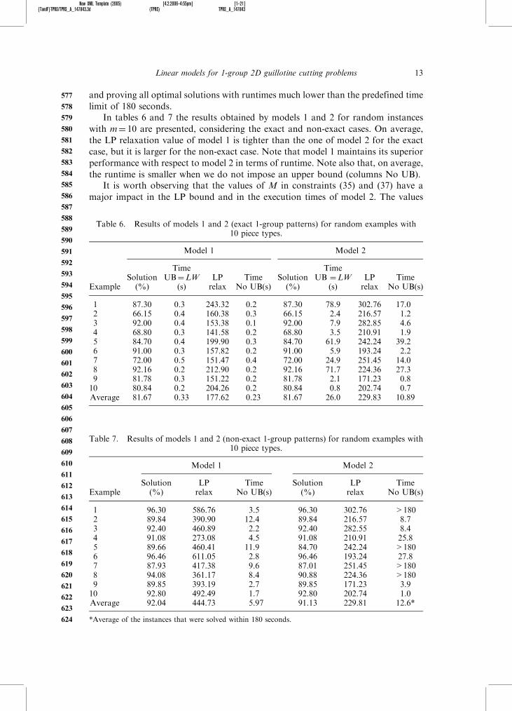
and proving all optimal solutions with runtimes much lower than the predefined time

limit of 180 seconds.In tables 6 and 7 the results obtained by models 1 and 2 for random instances

with m¼ 10 are presented, considering the exact and non-exact cases. On average,

the LP relaxation value of model 1 is tighter than the one of model 2 for the exact

case, but it is larger for the non-exact case. Note that model 1 maintains its superior

performance with respect to model 2 in terms of runtime. Note also that, on average,

the runtime is smaller when we do not impose an upper bound (columns No UB).It is worth observing that the values of M in constraints (35) and (37) have a

major impact in the LP bound and in the execution times of model 2. The values


Model 1 Model 2

ExampleSolution(%)

TimeUB¼LW

(s)LPrelax

TimeNo UB(s)

Solution(%)

TimeUB ¼LW

(s)LPrelax

TimeNo UB(s)

1 87.30 0.3 243.32 0.2 87.30 78.9 302.76 17.02 66.15 0.4 160.38 0.3 66.15 2.4 216.57 1.23 92.00 0.4 153.38 0.1 92.00 7.9 282.85 4.64 68.80 0.3 141.58 0.2 68.80 3.5 210.91 1.95 84.70 0.4 199.90 0.3 84.70 61.9 242.24 39.26 91.00 0.3 157.82 0.2 91.00 5.9 193.24 2.27 72.00 0.5 151.47 0.4 72.00 24.9 251.45 14.08 92.16 0.2 212.90 0.2 92.16 71.7 224.36 27.39 81.78 0.3 151.22 0.2 81.78 2.1 171.23 0.810 80.84 0.2 204.26 0.2 80.84 0.8 202.74 0.7Average 81.67 0.33 177.62 0.23 81.67 26.0 229.83 10.89

Table 7. Results of models 1 and 2 (non-exact 1-group patterns) for random examples with10 piece types.

Model 1 Model 2

ExampleSolution(%)

LPrelax

TimeNo UB(s)

Solution(%)

LPrelax

TimeNo UB(s)

1 96.30 586.76 3.5 96.30 302.76 >1802 89.84 390.90 12.4 89.84 216.57 8.73 92.40 460.89 2.2 92.40 282.55 8.44 91.08 273.08 4.5 91.08 210.91 25.85 89.66 460.41 11.9 84.70 242.24 >1806 96.46 611.05 2.8 96.46 193.24 27.87 87.93 417.38 9.6 87.01 251.45 >1808 94.08 361.17 8.4 90.88 224.36 >1809 89.85 393.19 2.7 89.85 171.23 3.910 92.80 492.49 1.7 92.80 202.74 1.0Average 92.04 444.73 5.97 91.13 229.81 12.6*

*Average of the instances that were solved within 180 seconds.


577

578

579

580

581

582

583

584

585

586

587

588

589

590

591

592

593

594

595

596

597

598

599

600

601

602

603

604

605

606

607

608

609

610

611

612

613

614

615

616

617

618

619

620

621

622

623

624


presented in tables 4, 5 and 6 were obtained using M equal to lmax and wmax in

constraints (35) and (37), respectively. If we use M equal to L and W in those

constraints, respectively, we would obtain much larger values for the LP relaxations

and longer execution times. For instance, the average LP relaxation value in table 5

would be 225.31 (instead of 164.41) and the average execution time would be

4.02 (instead of 2.62) and, in table 6, the average LP relaxation value would be

322.09 (instead of 229.83) and the average execution time would be 34.56 (instead

of 10.89).From table 7 we observe that in 4 out of the 10 instances tested, the upper

runtime limit of 180 seconds was reached when solving model 2 for the non-exact

case. The best objective value found when the model execution was interrupted is

indicated in the table within parentheses. We also carry out experiments with more

constrained random instances, that is, sampling (and then rounding) the quantities bifrom smaller intervals (e.g. [1, bL/licbW/wic/2]) than above ([1, bL/lic bW/wic]).

The relative performances of models 1 and 2 were similar to the ones observed in

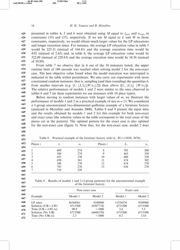
tables 6 and 7 (in these experiments we use instances with 10 piece types).Before moving to random instances with larger values of m, we illustrate the

performance of models 1 and 2 in a practical example of size m¼ 13. We considered

a 1-group unconstrained two-dimensional guillotine example of a furniture factory

(analysed in Morabito and Arenales 2000). Tables 8 and 9 present the input data

and the results obtained by models 1 and 2 for this example for both non-exact

and exact cases (the solution values in the table correspond to the total areas of the

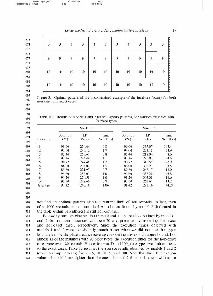
pieces cut in the pattern). The optimal pattern for the exact case is also optimal

for the non-exact case (figure 3). Note that, for the non-exact case, model 2 does

Table 8. Practical example of the furniture factory with (L, W)¼ (1850, 3670).

Pieces i li wi Pieces i Li wi

1 609 274 8 705 3002 380 274 9 465 3303 425 330 10 480 3304 650 361 11 674 3025 348 270 12 674 2706 705 270 13 636 2707 718 328

Table 9. Results of models 1 and 2 (1-group patterns) for the unconstrained exampleof the furniture factory.

Non exact case Exact case

Example Model 1 Model 2 Model 1 Model 2

LP relax 56244561 9349900 15534376 9349900Solution (UB¼LW) 6715500 (6507774) 6715500 6715500Time (UB¼LW) (s) 90.9 >1000 3.4 5.5Solution (No UB) 6715500 (6666170) 6715500 6715500Time (No UB) (s) 2.3 >1000 0.2 13.0


625

626

627

628

629

630

631

632

633

634

635

636

637

638

639

640

641

642

643

644

645

646

647

648

649

650

651

652

653

654

655

656

657

658

659

660

661

662

663

664

665

666

667

668

669

670

671

672


not find an optimal pattern within a runtime limit of 180 seconds. In fact, evenafter 1000 seconds of runtime, the best solution found by model 2 (indicated inthe table within parentheses) is still non-optimal.

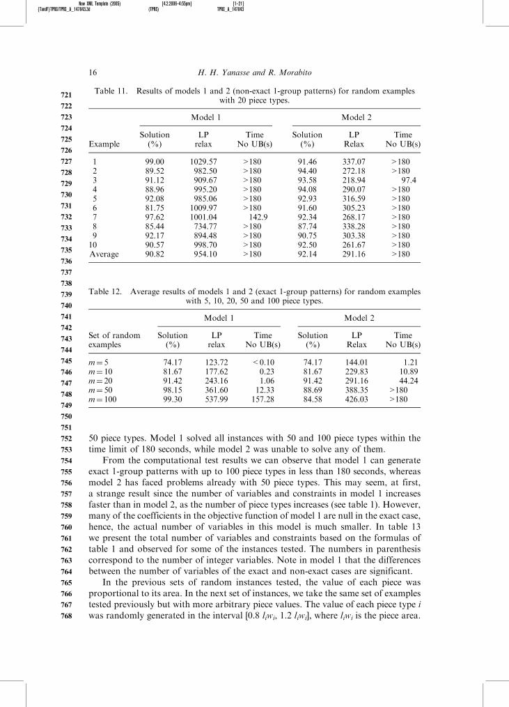
Following our experiments, in tables 10 and 11 the results obtained by models 1and 2 for random instances with m¼ 20 are presented, considering the exactand non-exact cases, respectively. Since the execution times observed withmodels 1 and 2 were, consistently, much better when we did not use the upperbound given by the plate area, we gave up considering any explicit upper bound. Foralmost all of the instances with 20 piece types, the execution times for the non-exactcases were over 180 seconds. Hence, for m¼ 50 and 100 piece types, we limit our teststo the exact cases. Table 12 resumes the average results obtained by models 1 and 2(exact 1-group patterns) for m¼ 5, 10, 20, 50 and 100. Note that the LP relaxationvalues of model 1 are tighter than the ones of model 2 for the data sets with up to

10 10 10 10 10 10 10 10 10 10 10

10 10 10 10 10 10 10 10 10 10 10

9 9 9 9 9 9 9 9 9 9 9

3 3 3 3 3 3 3 3 3 3 3

Figure 3. Optimal pattern of the unconstrained example of the furniture factory for bothnon-exact and exact cases.


Model 1 Model 2

ExampleSolution(%)

LPRelax

TimeNo UB(s)

Solution(%)

LPrelax

TimeNo UB(s)

1 99.00 274.64 0.8 99.00 337.07 145.42 93.00 235.12 1.7 93.00 272.18 23.93 85.44 268.61 0.8 85.44 218.94 8.64 92.16 224.49 1.1 92.16 290.07 24.55 90.72 244.48 1.2 90.72 316.59 127.96 86.00 204.02 1.5 86.00 305.23 23.57 89.60 221.97 0.7 89.60 268.17 12.08 94.60 235.07 1.0 94.60 338.28 46.89 91.20 224.58 1.0 91.20 303.38 16.610 92.50 298.60 0.8 92.50 261.67 13.2Average 91.42 243.16 1.06 91.42 291.16 44.24


673

674

675

676

677

678

679

680

681

682

683

684

685

686

687

688

689

690

691

692

693

694

695

696

697

698

699

700

701

702

703

704

705

706

707

708

709

710

711

712

713

714

715

716

717

718

719

720


50 piece types. Model 1 solved all instances with 50 and 100 piece types within thetime limit of 180 seconds, while model 2 was unable to solve any of them.

From the computational test results we can observe that model 1 can generateexact 1-group patterns with up to 100 piece types in less than 180 seconds, whereasmodel 2 has faced problems already with 50 piece types. This may seem, at first,a strange result since the number of variables and constraints in model 1 increasesfaster than in model 2, as the number of piece types increases (see table 1). However,many of the coefficients in the objective function of model 1 are null in the exact case,hence, the actual number of variables in this model is much smaller. In table 13we present the total number of variables and constraints based on the formulas oftable 1 and observed for some of the instances tested. The numbers in parenthesiscorrespond to the number of integer variables. Note in model 1 that the differencesbetween the number of variables of the exact and non-exact cases are significant.

In the previous sets of random instances tested, the value of each piece wasproportional to its area. In the next set of instances, we take the same set of examplestested previously but with more arbitrary piece values. The value of each piece type iwas randomly generated in the interval [0.8 liwi, 1.2 liwi], where liwi is the piece area.

Table 11. Results of models 1 and 2 (non-exact 1-group patterns) for random exampleswith 20 piece types.

Model 1 Model 2

ExampleSolution(%)

LPrelax

TimeNo UB(s)

Solution(%)

LPRelax

TimeNo UB(s)

1 99.00 1029.57 >180 91.46 337.07 >1802 89.52 982.50 >180 94.40 272.18 >1803 91.12 909.67 >180 93.58 218.94 97.44 88.96 995.20 >180 94.08 290.07 >1805 92.08 985.06 >180 92.93 316.59 >1806 81.75 1009.97 >180 91.60 305.23 >1807 97.62 1001.04 142.9 92.34 268.17 >1808 85.44 734.77 >180 87.74 338.28 >1809 92.17 894.48 >180 90.75 303.38 >18010 90.57 998.70 >180 92.50 261.67 >180Average 90.82 954.10 >180 92.14 291.16 >180

Table 12. Average results of models 1 and 2 (exact 1-group patterns) for random exampleswith 5, 10, 20, 50 and 100 piece types.

Model 1 Model 2

Set of randomexamples

Solution(%)

LPrelax

TimeNo UB(s)

Solution(%)

LPRelax

TimeNo UB(s)

m¼ 5 74.17 123.72 <0.10 74.17 144.01 1.21m¼ 10 81.67 177.62 0.23 81.67 229.83 10.89m¼ 20 91.42 243.16 1.06 91.42 291.16 44.24m¼ 50 98.15 361.60 12.33 88.69 388.35 >180m¼ 100 99.30 537.99 157.28 84.58 426.03 >180


721

722

723

724

725

726

727

728

729

730

731

732

733

734

735

736

737

738

739

740

741

742

743

744

745

746

747

748

749

750

751

752

753

754

755

756

757

758

759

760

761

762

763

764

765

766

767

768


We tested the models with instances with m¼ 10 piece types. In tables 14 and 15the results obtained by models 1 and 2 are presented considering the exact andnon-exact cases, respectively. Analysing the results of tables 14 and 15, we observeno significant difference compared with the results of tables 6 and 7. In fact, theexecution times seem to be slightly shorter, perhaps indicating that the case ofarbitrary values is easier to be solved. Also, no noticeable difference was identifiedin the LP relaxation bounds.

Finally, given that the size of model 1 depends on the number of differentlengths and widths, we tested the case where the total number of pieces (

Pmi¼1 bi)

remains the same and we vary only the number of piece types (m). We arbitrarily

Table 13. Number of variables and constraints in models 1 and 2 (exact andnon-exact cases).

Model 1 Model 2

Example Variables Constraints Variables Constraints

Vianna, m¼ 5, exact 69 (21) 171 223 (210) 228Vianna, m¼ 5, non-exact 164 (116) 171 223 (210) 144Ex. 1, m¼ 5, exact 88 (23) 227 367 (350) 372Ex.1, m¼ 5, non-exact 208 (143) 227 367 (350) 232Ex. 1, m¼ 10, exact 185 (38) 509 1020 (1000) 530Ex. 1, m¼ 10, non-exact 734 (588) 509 1020 (1000) 330Furniture, m¼ 13, exact 382 (62) 1072 999 (980) 383Furniture, m¼ 13, non-exact 1712 (1392) 1072 999 (980) 243Ex. 1, m¼ 20, exact 559 (69) 1674 2020 (2000) 540Ex. 1, m¼ 20, non-exact 4179 (3689) 1674 2020 (2000) 340Ex. 1, m¼ 50, exact 2089 (146) 6664 5020 (5000) 570Ex. 1, m¼ 50, non-exact 41189 (39246) 6664 5020 (5000) 370Ex. 1, m¼ 100, exact 3570 (226) 11502 10020 (10000) 620Ex. 1, m¼ 100, non-exact 140270 (136926) 11502 10020 (10000) 420

Table 14. Results of models 1 and 2 (exact 1-group patterns) for random examples with10 piece types with arbitrary values.

Model 1 Model 2

ExampleSolution(%)

LPrelax

TimeNo UB(s)

Solution(%)

LPrelax

TimeNo UB(s)

1 84.92 249.25 0.2 84.92 293.15 22.22 60.65 154.65 0.5 60.65 197.55 1.33 92.01 163.33 0.1 92.01 279.28 5.34 78.37 141.11 0.2 78.37 206.53 3.05 74.65 183.20 0.4 74.65 247.64 58.26 91.07 160.87 0.1 91.07 190.44 2.57 67.32 156.22 0.5 67.32 235.53 11.88 97.73 208.80 0.2 97.73 214.29 26.29 81.78 393.97 0.1 81.78 180.81 0.810 85.48 193.94 0.1 85.48 192.91 0.6Average 81.40 200.53 0.24 81.40 223.81 13.19


769

770

771

772

773

774

775

776

777

778

779

780

781

782

783

784

785

786

787

788

789

790

791

792

793

794

795

796

797

798

799

800

801

802

803

804

805

806

807

808

809

810

811

812

813

814

815

816


took example 1 of table 6 (with m¼ 10 piece types andPm

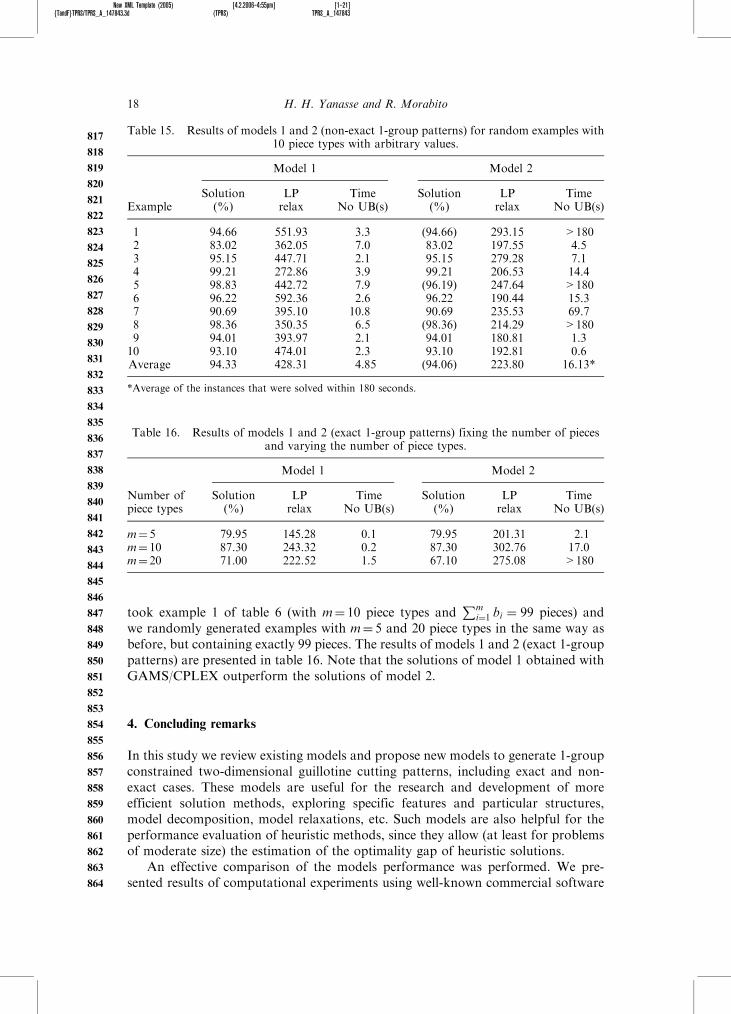
i¼1 bi ¼ 99 pieces) andwe randomly generated examples with m¼ 5 and 20 piece types in the same way asbefore, but containing exactly 99 pieces. The results of models 1 and 2 (exact 1-grouppatterns) are presented in table 16. Note that the solutions of model 1 obtained withGAMS/CPLEX outperform the solutions of model 2.

4. Concluding remarks

In this study we review existing models and propose new models to generate 1-groupconstrained two-dimensional guillotine cutting patterns, including exact and non-exact cases. These models are useful for the research and development of moreefficient solution methods, exploring specific features and particular structures,model decomposition, model relaxations, etc. Such models are also helpful for theperformance evaluation of heuristic methods, since they allow (at least for problemsof moderate size) the estimation of the optimality gap of heuristic solutions.

An effective comparison of the models performance was performed. We pre-sented results of computational experiments using well-known commercial software

Table 15. Results of models 1 and 2 (non-exact 1-group patterns) for random examples with10 piece types with arbitrary values.

Model 1 Model 2

ExampleSolution(%)

LPrelax

TimeNo UB(s)

Solution(%)

LPrelax

TimeNo UB(s)

1 94.66 551.93 3.3 (94.66) 293.15 >1802 83.02 362.05 7.0 83.02 197.55 4.53 95.15 447.71 2.1 95.15 279.28 7.14 99.21 272.86 3.9 99.21 206.53 14.45 98.83 442.72 7.9 (96.19) 247.64 >1806 96.22 592.36 2.6 96.22 190.44 15.37 90.69 395.10 10.8 90.69 235.53 69.78 98.36 350.35 6.5 (98.36) 214.29 >1809 94.01 393.97 2.1 94.01 180.81 1.310 93.10 474.01 2.3 93.10 192.81 0.6Average 94.33 428.31 4.85 (94.06) 223.80 16.13*

*Average of the instances that were solved within 180 seconds.

Table 16. Results of models 1 and 2 (exact 1-group patterns) fixing the number of piecesand varying the number of piece types.

Model 1 Model 2

Number ofpiece types

Solution(%)

LPrelax

TimeNo UB(s)

Solution(%)

LPrelax

TimeNo UB(s)

m¼ 5 79.95 145.28 0.1 79.95 201.31 2.1m¼ 10 87.30 243.32 0.2 87.30 302.76 17.0m¼ 20 71.00 222.52 1.5 67.10 275.08 >180


817

818

819

820

821

822

823

824

825

826

827

828

829

830

831

832

833

834

835

836

837

838

839

840

841

842

843

844

845

846

847

848

849

850

851

852

853

854

855

856

857

858

859

860

861

862

863

864


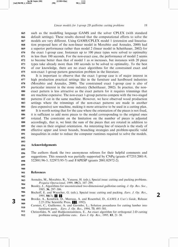
such as the modelling language GAMS and the solver CPLEX (with standarddefault settings). These results showed that the computational efforts to solve themodels are very different. Using GAMS/CPLEX model 1 (extension and linearisa-tion proposed here of the non-linear model in Morabito and Arenales, 2000) hada superior performance rather than model 2 (linear model in Scheithauer, 2002) forthe exact 1-group case. Instances up to 100 piece types were solved to optimalityin less than 180 seconds. For the non-exact case, the performance of model 2 seemsto become better than that of model 1 as m increases, but instances with 20 piecetypes take already more than 180 seconds to be solved to optimality. To the bestof our knowledge, there are no exact algorithms for the constrained exact andnon-exact 1-group pattern generation problem in the literature.

It is important to observe that the exact 1-group case is of major interest inhigh production practical settings like in the furniture and hardboard industries(Morabito and Arenales, 2000). The constrained exact 1-group case is also ofparticular interest in the stone industry (Scheithauer, 2002). In practice, the non-exact pattern is less attractive as the exact pattern for it requires trimmings thatare machine expensive. The non-exact 1-group patterns compete with the two-stagedpatterns if cut in the same machine. However, we have observed wood productionsettings where the trimmings of the non-exact patterns are made in another(less expensive) saw machine, making it more attractive to be used in a cutting plan.

It is worth noting that for the case where the orientation of the pieces is not fixed,it is sufficient to add more pieces to the model corresponding to the original onesrotated. The constraint on the limitation on the number of pieces is adjustedaccordingly, that is, we limit the sum of the pieces that are rotated in addition tothe ones in their original orientation. An interesting line of research is the study ofeffective upper and lower bounds, branching strategies and problem-specific validinequalities in order to reduce the computer runtimes required to solve the models.

Acknowledgements

The authors thank the two anonymous referees for their helpful comments andsuggestions. This research was partially supported by CNPq (grants 477255/2001-9,522881/96-3, 522973/95-7) and FAPESP (grants 2001/02972-2).

References

Arenales, M., Morabito, R., Yanasse, H. (eds.), Special issue: cutting and packing problems.Pesquisa Operacional, 1999, 19(2), 107–299.

Beasley, J., Algorithms for unconstrained two-dimensional guillotine cutting. J. Op. Res. Soc.,1985, 36, 297–306.

Bischoff, E. and Waescher, G. (eds.), Special issue: cutting and packing. Euro. J. Op. Res.,1995, 84(3), 22–22.

Brooke, A., Kendrick, D., Meeraus, A. and Rosenthal, D., GAMS:A User’s Guide, Release2.25 (The Scientific Press, 222, 1992).

Carnieri, C., Guillermo, A. and Gavinho, L., Solution procedures for cutting lumber intofurniture parts.. Euro. J. Op. Res., 1994, 73, 495–501.

Christofides, N. and Hadjiconstantinou, E., An exact algorithm for orthogonal 2-D cuttingproblems using guillotine cuts.. Euro J. Op. Res., 1995, 83, 21–38.


865

866

867

868

869

870

871

872

873

874

875

876

877

878

879

880

881

882

883

884

885

886

887

888

889

890

891

892

893

894

895

896

897

898

899

900

901

902

903

904

905

906

907

908

909

910

911

912

proofreader

Text Box

2

proofreader

Text Box

3


Dowsland, K. and Dowsland, W., Packing problems. Euro. J. Op. Res., 1992, 56, 2–14.Dyckhoff, H. and Finke, U., Cutting and Packing in Production and Distribution: Typology

and Bibliography, 1992 (Springler-Verlag Co.: Heidelberg, Germany).Dyckhoff, H., Scheithauer, G. and Terno, J., Cutting and packing, in Annotated Bibliographies

in Combinatorial Optimisation, edited by M. Amico, F. Maffioli, and S. Martello(John Wiley & Sons, New York, NY, 1997)393–414.

Dyckhoff, H. and Waescher, G. (eds.), Special issue: cutting and packing. Euro. J. Op. Res.,1990, 44(2), 22–22.

Farley, A., Practical adaptations of the Gilmore-Gomory approach to cutting stock problems.OR Spectrum, 1983, 10, 113–123.

Foronda, S. and Carino, H., a heuristic approach to the lumber allocation and manufacturingin hardwood dimension and furniture manufacturing. Euro. J. Op. Res., 1991, 54,151–162.

Gilmore, P. and Gomory, R., Multistage cutting stock problems of two and more dimensions.Op. Res., 1965, 14, 94–120.

Harjunkoski, I., Porn, R., Westerlund, T. and Skifvars, H., Different strategies forsolving bilinear integer non-linear programming problems with convex transformations.Computers & Chem. Eng., 1997, 21, 487–492.

Hifi, M., The DH/KD algorithm: a hybrid approach for unconstrained two-dimensionalcutting problems. Euro. J. Op. Res., 1997, 97(1), 41–52.

Hifi, M. (ed), Special issue on cutting and packing. Studia Informatica Universalis, 2002,2, 1–161.

Hifi, M. and Roucairol, C., Approximate and exact algorithms for constrained (un)weightedtwo-dimensional two-staged cutting stock problems. J. Combin. Optim., 2001, 5,465–494.

Hinxman, A., The trim-loss and assortment problems: a survey. Euro. J. Op. Res., 1980,5, 8–18.

Lirov, Y. (ed), Special issue: cutting stock: geometric resource allocation, Math. & Comp.Mod., 1992, 16(1), 22–22.

Lodi, A., Martello, S. and Monaci, M., Two-dimensional packing problems: a survey.Euro. J. Op. Res., 2002, 141, 241–252.

Lodi, A. and Monaci, M., Integer programming models for 2-staged two-dimensionalknapsack problems. Math. Prog., 2003, 94, 257–278.

Martello, S. (ed), Special issue: knapsack, packing and cutting. Part I: One-dimensionalknapsack problems. INFOR, 1994a, 32(3), 22–22.

Martello, S. (ed), Special issue: knapsack, packing and cutting. Part II: Multidimensionalknapsack and cutting stock problems. INFOR, 1994b, 32(4), 22–22.

Morabito, R. and Arenales, M., Staged and constrained two-dimensional guillotinecutting problems: an and/or-graph approach. Euro. J. Op. Res., 1996, 94, 548–560.

Morabito, R. and Arenales, M., Optimising the cutting of stock plates in a furniture company.Int. J. Prod. Res., 2000, 38(12), 2725–2742.

Morabito, R. and Garcia, V., The cutting stock problem in a hardboard industry: a case study.Computers & Operations Research, 1998, 25(6), 469–485.

Mukhacheva, E.A. (ed), Decision making under conditions of uncertainty: Cutting–packingproblems, 1997 (The International Scientific Collection: Ufa, Russia).

Riehme, J., Scheithauer, G. and Terno, J., The solution of two-stage guillotine cuttingstock problems having extremely varying order demands. Euro. J. Op. Res., 1996, 91,543–552.

Scheithauer, G., On a two-dimensional guillotine cutting problem. Presented at IFORS 2002,Edinburgh, UK, 2002.

SICUP, Special interest group on cutting and packing, 2004. Available online at: http://www.apdio.pt/sicup/(accessed 22222).

Sweeney, P. and Paternoster, E., Cutting and packing problems: a categorised, application-oriented research bibliography. J. Op. Res. Soc., 1992, 43, 691–706.

Vianna, A.C., Arenales, M. and Gramani, M.C., Two-stage and constrained two-dimensionalguillotine cutting problems. Working paper, Universidade de Sao Paulo, Brazil, 2002(submitted for publication).


913

914

915

916

917

918

919

920

921

922

923

924

925

926

927

928

929

930

931

932

933

934

935

936

937

938

939

940

941

942

943

944

945

946

947

948

949

950

951

952

953

954

955

956

957

958

959

960

proofreader

Text Box

2

proofreader

Text Box

2

proofreader

Text Box

2

proofreader

Text Box

2

proofreader

Text Box

2

proofreader

Text Box

2

proofreader

Text Box

4


Yanasse, H.H. and Katsurayama, D.M., Checkerboard patterns: proposals for its generation.Int. Trans. Op. Res., 2005, 12, 21–45.

Yanasse, H.H., Zinober, A. and Harris, R., Two-dimensional cutting stock with multiplestock sizes. J. Op. Res. Soc., 1991, 42(8), 673–683.

Waescher, G. and Gau, T., Heuristics for the integer one-dimensional cutting stock problem:a computational study. OR Spectrum, 1996, 18, 131–144.

Wang, P. and Waescher, G. (eds.), Special issue on cutting and packing problems. Euro. J.Op. Res., 2002, 141, 239–469.


961

962

963

964

965

966

967

968

969

970

971

972

973

974

975

976

977

978

979

980

981

982

983

984

985

986

987

988

989

990

991

992

993

994

995

996

997

998

999

1000

1001

1002

1003

1004

1005

1006

1007

1008

TPRS A 147843 1. - dep.ufscar.br proofs.pdf · AUTHOR QUERIES Journal id: TPRS_A_147843...

Documents

Transcript of TPRS A 147843 1. - dep.ufscar.br proofs.pdf · AUTHOR QUERIES Journal id: TPRS_A_147843...