University of Canberra

Toxicology of the Amanita phalloides

(Death Cap) Mushroom

Detection of Amatoxins and Phallotoxins by Ultra-

Performance Liquid Chromatography Coupled with

Tandem Mass Spectrometry

Ashlea Norton

Bachelor of Applied Science in Forensic Studies (UC)

National Centre for Forensic Studies (NCFS)

University of Canberra ACT

A thesis submitted in partial fulfilment of the requirements for the

degree of Bachelor of Applied Science (Honours) at the University of

Canberra

December 2014

ii

Acknowledgements:

I would like to thank all the staff at the ACT Government Analytical Laboratory for

providing me with the means to carry out this project, assisting me with obtaining blood

specimens and other materials needed for my project, generally providing encouragement and

support, and for making me feel like a part of the team.

I would also like to thank the staff at the University of Canberra, who were always willing to

provide feedback and ideas. Thankyou to Michelle Gahan, who was so helpful and

understanding when things went wrong. To my fellow honours students, thankyou for being

there when I needed support, encouragement or simply an opportunity to take a break from it

all. I would also like to thank the PhD students who shared their honours experiences and

helped me see the light at the end of the tunnel.

Thankyou to my family and friends, who provided no shortage of encouragement and pushed

me to keep going in the most difficult times. Despite living in a different state, my friends

have always been there when I needed them most. To my mother, who has always believed in

me, thankyou for pushing me to accomplish my goals, being my rock when I felt the

pressure, and for making me believe in myself.

Finally, I would like to thank my supervisors Tamsin Kelly, Ian Whittall and Joanne Giaccio,

who brought this project to my attention, provided me with everything I needed and without

whom none of this would have been possible. Thankyou for all your advice, patience and

support throughout my project. Working with you has been a fantastic experience for which I

will always be grateful.

iii

Abstract

The increasing number of Amanita phalloides poisoning cases in Australia and lack of

efficient treatment options has emphasised the need for detection methods which can be

applied in forensic and clinical toxicology. In this study, an existing method utilised by

Nomura et al. [1]

was adapted for the detection of A. phalloides toxins, α-amanitin, β-amanitin

and phalloidin, in whole blood specimens using ultra-performance liquid chromatography

coupled with tandem mass spectrometry (UPLC-MS/MS). Various parameters were

evaluated in order to develop an optimised method, which was then validated.

Optimisation of the MRM parameters was conducted using MS/MS with an electrospray

interface in positive ionisation mode. This mode was found to give the greatest number of

stable transitions and far greater sensitivity than negative ionisation mode. Resolution of the

two amanitins was achieved using a Waters ACQUITY UPLC BEH C18 column (2.1 mm x

150 mm) and a mobile phase combination of 5 mM ammonium formate with 0.05% formic

acid : 0.1% formic acid in water at a flow rate of 0.4 mL/min. The total run time of the

method was 8 minutes. Two internal standards, virginiamycin B and rifampicin, were

evaluated with rifampicin being chosen as the internal standard.

Samples were diluted prior to undergoing solid-phase extraction. The sample preparation

method utilised a dilution step followed by SPE. Several columns were trialled, with the UCT

Clean Up C18 column providing the best recovery. The SPE method was adapted from that

outlined in Nomura et al. [1]

The overall developed method was validated according to NATA guidelines [2]

and methods

outlined by Shah et al. [3]

The parameters evaluated included selectivity, matrix effects,

linearity, recovery, sensitivity, precision and limits of detection and quantification. The

method produced good selectivity for each analyte, however significant matrix effects were

encountered for the analytes which affected further results. Linearity studies were performed

over the range of 25-500 ng/mL for the amanitins and 5-100 ng/mL for phalloidin, and gave

correlation coefficients of 0.9731, 0.9825 and 0.9872 for α-amanitin, β-amanitin and

phalloidin respectively. Average recoveries ranged from 79.46%-107.99% for α-amanitin,

46.96-62.19% for β-amanitin and 6.62-12.45% for phalloidin, suggesting the extraction

method needs further improvement. The method exhibited poor sensitivity for the analytes,

with slopes of 0.0031, 0.0022 and 0.0002 for α-amanitin, β-amanitin and phalloidin

iv

respectively. The method was found to be precise for each of the analytes and showing no

significant difference between data points, with p-values of 0.4279 for α-amanitin, 0.7265 for

β-amanitin and 0.7814 for phalloidin. Limits of detection were determined to be 25 ng/mL for

both amanitins and 20 ng/mL for phalloidin. Limits of quantification were determined to be

75 ng/mL for the amanitins and 60 ng/mL for phalloidin. Overall, the developed method did

not pass validation, however offers a good basis for further work.

v

Table of Contents

Acknowledgements: ................................................................................................................... ii

Abstract .................................................................................................................................... iii

List of Appendices ................................................................................................................... vii

List of Tables ......................................................................................................................... viii

List of Figures ............................................................................................................................ x

1. Introduction ............................................................................................................................ 1

1.1. Pharmacology and Toxicology of Cyclopeptides ........................................................... 1

1.2. Introduction to Australia and Spread of A. phalloides .................................................... 3

1.3. Clinical Treatment of A. phalloides Poisoning ............................................................... 5

1.4. Review of Methods in Literature for Detection of Amatoxins and Phallotoxins ........... 5

1.4.1. Sample Preparation ................................................................................................... 6

1.4.2. Liquid Chromatography ......................................................................................... 15

1.4.3. Mass Spectrometry ................................................................................................. 17

1.5. Aims of Study................................................................................................................ 24

2. Materials and Methods ......................................................................................................... 25

2.1. General .......................................................................................................................... 25

2.1.1. Chemicals and Reagents ......................................................................................... 25

2.1.2. Preparation of Buffers ............................................................................................ 26

2.1.3. Source of Blood Specimens .................................................................................... 26

2.1.4. Glassware and Syringes .......................................................................................... 26

2.1.5. UPLC-MS/MS ........................................................................................................ 27

2.1.6. Solid Phase Extraction ............................................................................................ 27

2.1.7. Other Instrumentation ............................................................................................. 28

2.2. Method Development .................................................................................................... 29

2.2.1. Characterisation ...................................................................................................... 29

2.2.2. Choice of Mobile Phase .......................................................................................... 30

2.2.3. Choice of Gradient System ..................................................................................... 31

2.2.4. Choice of Reconstitution Solvent ........................................................................... 31

2.2.5. Sample Preparation ................................................................................................. 31

2.2.6. Choice of Internal Standard .................................................................................... 32

2.2.7. Parameters for Final Developed Method ................................................................ 32

vi

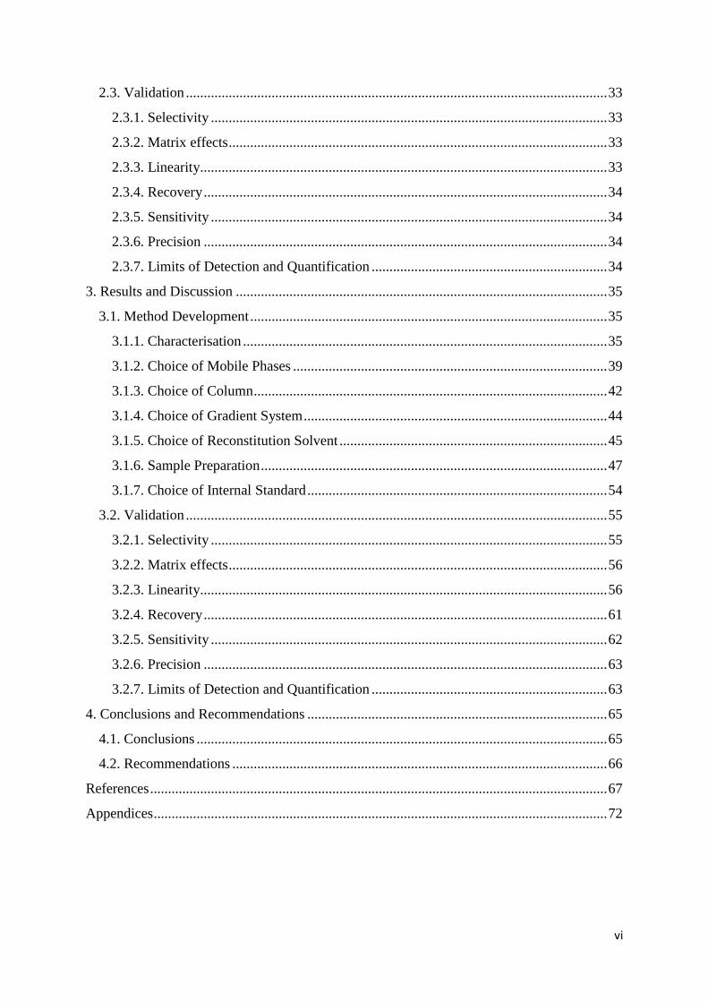
2.3. Validation ...................................................................................................................... 33

2.3.1. Selectivity ............................................................................................................... 33

2.3.2. Matrix effects .......................................................................................................... 33

2.3.3. Linearity.................................................................................................................. 33

2.3.4. Recovery ................................................................................................................. 34

2.3.5. Sensitivity ............................................................................................................... 34

2.3.6. Precision ................................................................................................................. 34

2.3.7. Limits of Detection and Quantification .................................................................. 34

3. Results and Discussion ........................................................................................................ 35

3.1. Method Development .................................................................................................... 35

3.1.1. Characterisation ...................................................................................................... 35

3.1.2. Choice of Mobile Phases ........................................................................................ 39

3.1.3. Choice of Column ................................................................................................... 42

3.1.4. Choice of Gradient System ..................................................................................... 44

3.1.5. Choice of Reconstitution Solvent ........................................................................... 45

3.1.6. Sample Preparation ................................................................................................. 47

3.1.7. Choice of Internal Standard .................................................................................... 54

3.2. Validation ...................................................................................................................... 55

3.2.1. Selectivity ............................................................................................................... 55

3.2.2. Matrix effects .......................................................................................................... 56

3.2.3. Linearity.................................................................................................................. 56

3.2.4. Recovery ................................................................................................................. 61

3.2.5. Sensitivity ............................................................................................................... 62

3.2.6. Precision ................................................................................................................. 63

3.2.7. Limits of Detection and Quantification .................................................................. 63

4. Conclusions and Recommendations .................................................................................... 65

4.1. Conclusions ................................................................................................................... 65

4.2. Recommendations ......................................................................................................... 66

References ................................................................................................................................ 67

Appendices ............................................................................................................................... 72

vii

List of Appendices

Appendix 1: Drug Mixtures used for Selectivity .................................................................... 73

Appendix 2: Linearity Plots .................................................................................................... 75

Appendix 3: Data Generated from ANOVA Single Factor Analysis ..................................... 78

Appendix 4: Signal to noise (S/N) Data ................................................................................. 81

viii

List of Tables

Table 1.1. Sample preparation and extraction methods for mushroom tissue. ......................... 7

Table 1.2. Sample preparation and extraction methods for biological specimens. ................... 8

Table 1.3. Solid phase extraction methods and results from amatoxin literature for mushroom

tissue. ....................................................................................................................................... 12

Table 1.4. Solid-phase extraction methods and results from amatoxin literature for biological

matrices. ................................................................................................................................... 13

Table 1.5. LC methods and parameters encountered in literature for amatoxins.................... 16

Table 1.6. LC-MS and LC-MS/MS parameters and fragment ions for amatoxins and

phallotoxins in literature. ......................................................................................................... 20

Table 1.7. LC-TOF-MS parameters and fragment ions for amatoxins and phallotoxins in

literature. .................................................................................................................................. 21

Table 1.8. Limits of detection and quantification for direct mushroom extracts. ................... 22

Table 1.9. Limits of detection and quantification for biological specimen extracts. .............. 23

Table 2.1. Preparation of stock solutions in 1 mL methanol................................................... 25

Table 2.2. Analysis of standards using ESI- mode. ................................................................ 29

Table 2.3. Analysis of standards using ESI+ mode. ............................................................... 30

Table 2.4. Mobile phase combinations trialled in method development. ............................... 30

Table 3.1. Transitions and parameters found using ESI+ mode. ............................................ 36

Table 3.2. Transitions and parameters found using ESI- mode. ............................................. 37

Table 3.3. Transitions and parameters found using ESI+ mode upon increasing concentration

of analytes. ............................................................................................................................... 38

Table 3.4. Comparison of peak height of quantifier ion at 25 ng/mL within standard mix

using ESI+ and ESI- mode. ...................................................................................................... 39

Table 3.5. Mobile phases used and optimal parameters found for each. ................................ 40

Table 3.6. Columns used and optimal parameters found for each. ......................................... 42

Table 3.7. Extraction efficiencies of standards at 75 ng/mL (ESI- mode). ............................. 49

Table 3.8. Extraction efficiencies of standards at 200 ng/mL (ESI+ mode). .......................... 50

Table 3.9. Methods and variations trialled for SPE. ............................................................... 52

Table 3.10. Differences in peak area resulting from various extraction methods. .................. 53

Table 3.11. Comparison of peak area for quantifier ion using 100 ng/mL pure solutions with

and without filtering step. ........................................................................................................ 54

ix

Table 3.12. Comparison of internal standards within a 25 ng/mL mixture. ........................... 55

Table 3.13. Average extraction efficiency and recovery values for α-amanitin, β-amanitin

and phalloidin........................................................................................................................... 62

x

List of Figures

Figure 1.1. Chemical structures of α-amanitin and β-amanitin ................................................ 2

Figure 1.2. Chemical structure of phalloidin ............................................................................ 3

Figure 1.3. Comparison of A. phalloides and V. volvacea ........................................................ 5

Figure 1.4. Basic principle of solid phase extraction .............................................................. 11

Figure 1.5. Mechanism of electrospray ionisation .................................................................. 18

Figure 1.6. Mechanism of single ion monitoring .................................................................... 19

Figure 1.7. Mechanism of multiple reaction monitoring ........................................................ 19

Figure 3.1. Possible fragment for m/z 259 .............................................................................. 35

Figure 3.2. Separation of α-amanitin and β-amanitin using different mobile phases ............. 41

Figure 3.3. Separation of α-amanitin and β-amanitin using different columns ...................... 43

Figure 3.4. Gradient program developed for amatoxin and phallotoxin analysis. .................. 44

Figure 3.5. Investigation of reconstitution solvent ................................................................. 46

Figure 3.6. Linearity plots for α-amanitin, β-amanitin and phalloidin. .................................. 58

Figure 3.7. Residual plots for α-amanitin, β-amanitin and phalloidin. ................................... 60

1

1. Introduction

Around the world, there are as many as 5000-6000 species of mushroom, of which only 1000

are named [4,5]

. Toxic mushrooms make up only a small number of these, however are still a

major concern as they are often mistaken for edible mushrooms [5,6]

. Toxic mushrooms can be

classified into seven categories based on the toxins that they contain; these are cyclopeptides,

gyromitrin, coprine, muscarine, ibotenic acid-muscimol, psilocybin and gastrointestinal

irritants [6]

.

Of the toxic mushrooms outlined above, those of the cyclopeptide group of mushrooms have

the highest toxicity. The most lethal mushroom in this category is Amanita phalloides [6-9]

.

This mushroom is also known as the “death cap” mushroom, and is attributed to 50% of all

mushroom poisonings and approximately 90% of mushroom related fatalities [10-12]

. The

toxins of A. phalloides have a delayed onset of symptoms, which is problematic as early

diagnosis is essential for treatment to be effective [1,13,14]

.

There are four typical phases of A. phalloides mushroom poisoning [7,12]

. The first is the

asymptomatic phase, occurring between 0-18 hours after ingestion [7,12]

. Gastroenteritis

ensues between 6-24 hours after ingestion; this is referred to as the gastrointestinal phase

[7,12]. Symptoms observed during this phase include abdominal pain, nausea, vomiting, watery

or bloody diarrhoea, dehydration and impaired renal and hepatic function [11,12]

. Between 1-7

days after ingestion, there is an apparent remission phase in which gastrointestinal symptoms

disappear while progressive cell damage occurs in the liver and kidneys [7,11,12]

. After 7 days,

complete renal and hepatic failure occurs, leading to convulsions, irreversible coma and

possible death [7,11,12]

.

1.1. Pharmacology and Toxicology of Cyclopeptides

There are two main classes of cyclopeptides in A. phalloides mushrooms, amatoxins and

phallotoxins [10]

. Amatoxins are bicyclic octapeptides, and are the primary cause of toxicity

[1,5,10]. There are nine known amatoxins, the most significant of these being α-amanitin and β-

amanitin (Figure 1.1) [10,14]

. The molecular weights of α-amanitin and β-amanitin are 918 and

919 Daltons respectively [1,13]

. Amatoxins are rapidly absorbed in the intestines and do not

bind to plasma proteins, instead remaining free in the circulatory system [6,11]

. The

metabolism of amatoxins in the body is not known [15]

. Amatoxins are excreted relatively

rapidly, with 80-85% of amatoxins being excreted in urine and less than 10% excreted in bile

2

within the first six hours [11,16]

. When symptoms begin to develop, the concentration of

amatoxins in urine ranges from 50-500 ng/mL [13]

. Leite et al. [11]

observed that amatoxins

were completely removed from urine after 24-36 hours in patients with forced diuresis,

however remained in the gastric and duodenal systems for a further 24-48 hours.

Figure 1.1. Chemical structures of α-amanitin and β-amanitin. [17]

Amatoxins act by binding to the enzyme RNA polymerase II in hepatocytes, which in turn

inhibits transcription by decreasing the amount of mRNA available for protein synthesis

causing cell necrosis [1,11,12,14,18,19]

. Amatoxins are 10-20 times more toxic than phallotoxins,

but have a greater latency period [10,20]

. Amatoxins are highly stable and are not affected by

heat or dryness, meaning they cannot be denatured by cooking or freezing processes [1,6,7]

.

This is significant as most encounters with these toxins arise from ingestion of A. phalloides

mushrooms. Wieland [21]

reports that there is approximately 8 mg of α-amanitin, 5 mg of β-

amanitin and 10 mg of phalloidin per 100 g of mushroom tissue. The lethal dose of amatoxins

is very low (approximately 0.1 mg/kg), meaning a serving of less than 50g of A. phalloides

mushrooms could be potentially fatal [21]

.

3

Phallotoxins are bicyclic heptapeptides, of which there are six types [10]

. Phalloidin is the

primary phallotoxin of A. phalloides mushrooms, and has a molecular weight of 788 Daltons

(Figure 1.2). Phallotoxins are less toxic than amatoxins, and do not have a toxic effect if

ingested as they are not absorbed in the gastrointestinal tract [1,5]

. They are therefore not

considered to contribute to A. phalloides toxicity. However, it should be noted that when

administered parenterally (through intravenous injection) phallotoxins bind to F-actin and

prevent depolymerisation to G-actin, altering the cell membrane of enterocytes [22]

. Toxic

effects from parenteral administration are rapid, causing fatality in approximately 1-2 hours

in mice [23]

. Phallotoxins are less stable than amatoxins and are denatured with heat, so are

eliminated with cooking [1]

. However, when determining potential ingestion of A. phalloides

mushrooms, the presence of phalloidin is a useful biomarker for specific identification of the

mushroom ingested [1]

.

Figure 1.2. Chemical structure of phalloidin. [17]

1.2. Introduction to Australia and Spread of A. phalloides

A. phalloides is the leading cause of mushroom poisonings across the world [10-12]

. This

species originates from Europe, and has since been introduced to North America, Africa, Asia

and Australia; it is now one of the most predominant toxic species of mushroom across the

world [24]

.

4

In Australia, these mushrooms are most commonly encountered in south eastern regions [7]

.

A. phalloides was first introduced to Canberra in 1961, and has since spread to regions of

Victoria and New South Wales [7]

. Their introduction in Australia is linked to the importation

of oak trees, due to the symbiotic mycorrhizal relationship between A. phalloides and the

roots of these trees [7,24]

. There is a growing concern that this relationship will expand to

involve trees native to Australia [7,24]

. There have been reported cases of some Eucalyptus

species developing mycorrhizal relationships with other Amanita species across the world [7]

.

In Africa a direct association between some Eucalyptus species and A. phalloides has been

observed [7]

. If such a relationship were to develop between the native Eucalyptus species of

Australia and A. phalloides, this could lead to the mushroom becoming widespread across the

country. This in turn would significantly increase the occurrence of A. phalloides poisoning

as the affected areas may no longer be limited to southern regions of Australia.

1.2.1. Cases of A. phalloides Poisoning in Australia

There have been many recent cases of A. phalloides poisoning in Australia. Over the last

fourteen years there have been four reported fatal cases and 12 non-fatal cases, with an

additional four cases occurring earlier this year [25,26]

. The A. phalloides mushroom grows

seasonally in Summer and Autumn, and every year around this time health warnings are

issued by state health departments [12]

. Most often, A. phalloides is mistaken for the

traditional Chinese mushroom Volvariella volvacea, also known as the straw mushroom

(Figure 1.3) [7]

. For this reason, it is generally ethnic cultures who are more at risk of A.

phalloides poisoning [27]

. In 2012 a woman in the Australian Capital Territory (ACT) visiting

from China was placed in intensive care after preparing a family meal from A. phalloides,

mistaking the mushrooms for V. volvacea [28]

. A more serious case occurred at the end of

2011, when a Chinese chef prepared a meal for three of his colleagues at a New Year’s Eve

party [29,30]

. He and one of his colleagues died from liver failure while the other two were

hospitalised [29]

. While it was assured that these mushrooms were not served to members of

the public, this incident raised the concern of potential public exposure to poisonous

mushrooms [29]

. Earlier this year four people were admitted to hospital after ingesting these

mushrooms, three of which had shared the same meal [31]

. Two of these victims suffered

severe liver damage as a result [31]

. Initially there were concerns that these mushrooms had

been sourced from a local supermarket, however these concerns were later quashed [26]

.

Incidences of A. phalloides poisoning appear to be increasing in the ACT, and it is therefore

essential that health warnings be issued regularly [12]

.

5

Figure 1.3. Comparison of A. phalloides (left) and V. volvacea (right). [28]

1.3. Clinical Treatment of A. phalloides Poisoning

There are a variety of treatment methods available for A. phalloides poisoning, however early

administration is key for their success. There are three main stages of treatment for A.

phalloides poisoning – preliminary medical care, supportive measures and specific therapies

[14]. These methods aim to prevent circulation of amatoxins within the body and inhibit

uptake of amatoxins by hepatocytes [6,7]

. This is primarily achieved through methods which

reduce absorption of amatoxins and increase excretion [14,32]

. If these treatments all prove

ineffective, the only other option is liver transplantation [6,8,14]

. In the ACT, Legalon ® SIL, a

silibinin derivative, is used as an antidote [12]

. This drug acts by competing with the same

active site on hepatocytes as the amatoxins, and hence prevents uptake of the toxins [16]

.

Despite this, there is currently no blood test available in Australia which can confirm the

presence of amatoxins [12]

. This significantly limits treatment options, particularly considering

the extended latency period of amatoxins and the delayed onset of symptoms [12]

. Early

detection is therefore essential in clinical cases to allow treatment to be implemented at the

earliest possible opportunity.

1.4. Review of Methods in Literature for Detection of Amatoxins and Phallotoxins

The general analytical method employed in toxicological analysis of a biological specimen

involves three main stages. Firstly, sample preparation is used to purify the specimen and

isolate the desired analyte from other constituents [33]

. This step also allows for concentration

of the analytes for better detection, and reduces the possibility of matrix interference [33,34]

.

6

Secondly, a separation method is employed to differentiate components within a sample. This

is usually achieved through chromatography methods. Finally, identification (and

quantification where possible) of the analytes is performed. This is most often achieved

through the use of detection methods such as mass spectrometry.

There are currently very few methods which have been successfully utilised for amatoxin

detection, with none pertaining to whole blood specimens. Methods which have been

previously evaluated for amatoxin screening in urine, plasma and serum specimens include

the Meixner test [35,36]

and immunoassays such as radioimmunoassay (RIA) and enzyme

linked immunosorbent assay (ELISA) [11,37]

. Confirmatory testing was performed in one study

by capillary electrophoresis (CE) [10]

, but the amatoxin literature overwhelmingly favours the

use of liquid chromatography (LC) methods [1,5,9-11,38]

. Of the 14 articles found that present a

method for amatoxin analysis, 13 utilise an LC method. Of these articles, eight demonstrate

an analytical method for amatoxins within a biological matrix while the remaining articles

analyse the mushroom specimen itself. Each of these methods was investigated to determine

which method could provide the most potential for analysis of amatoxins in whole blood.

The use of whole blood for amatoxin analysis would be useful for both clinical and post-

mortem diagnosis. It is therefore essential that a rapid and sensitive method for amatoxin

detection in whole blood be developed. Rapid analysis is particularly important considering

the limited time frame in which liver damage can ensue. Sensitivity is also of great

importance given the low lethal dose of amanitins (0.1 mg/kg) [7,16]

.

1.4.1. Sample Preparation

Sample preparation generally involves an extraction technique as biological matrices often

cannot be directly injected onto an analytical instrument, and hence require clean-up prior to

analysis. Sometimes it is necessary to have additional preparation steps such as dilution or

protein precipitation prior to extraction. In the majority of the literature for amatoxins, solid

phase extraction (SPE) was the chosen extraction method but sample preparation steps prior

to extraction were highly variable. It is important to evaluate sample preparation steps

particularly for whole blood analysis, as many components within this matrix have the

potential to interfere with analysis. As no whole blood analysis for amatoxins has previously

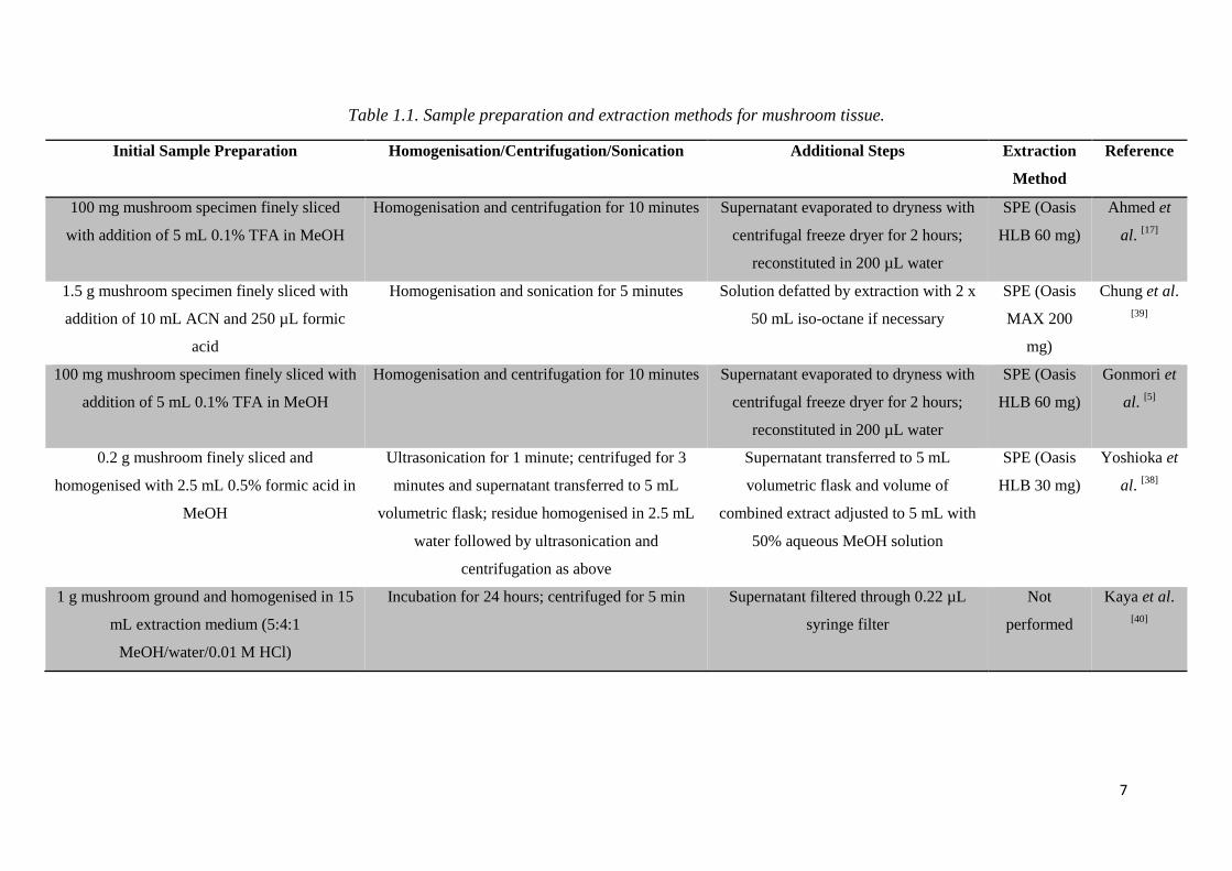
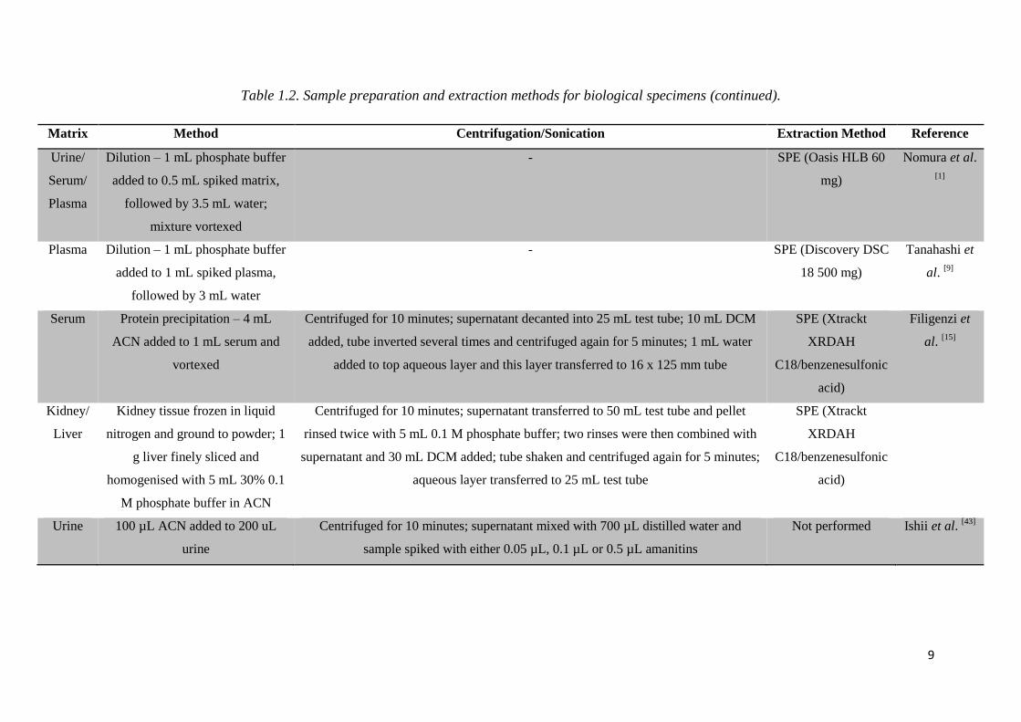
been reported, methods for various other matrices were investigated and compared. Those

performed on mushroom tissue (Table 1.1) are compared separately from those performed on

biological matrices (Table 1.2).

7

Table 1.1. Sample preparation and extraction methods for mushroom tissue.

Initial Sample Preparation Homogenisation/Centrifugation/Sonication Additional Steps Extraction

Method

Reference

100 mg mushroom specimen finely sliced

with addition of 5 mL 0.1% TFA in MeOH

Homogenisation and centrifugation for 10 minutes Supernatant evaporated to dryness with

centrifugal freeze dryer for 2 hours;

reconstituted in 200 µL water

SPE (Oasis

HLB 60 mg)

Ahmed et

al. [17]

1.5 g mushroom specimen finely sliced with

addition of 10 mL ACN and 250 µL formic

acid

Homogenisation and sonication for 5 minutes Solution defatted by extraction with 2 x

50 mL iso-octane if necessary

SPE (Oasis

MAX 200

mg)

Chung et al.

[39]

100 mg mushroom specimen finely sliced with

addition of 5 mL 0.1% TFA in MeOH

Homogenisation and centrifugation for 10 minutes Supernatant evaporated to dryness with

centrifugal freeze dryer for 2 hours;

reconstituted in 200 µL water

SPE (Oasis

HLB 60 mg)

Gonmori et

al. [5]

0.2 g mushroom finely sliced and

homogenised with 2.5 mL 0.5% formic acid in

MeOH

Ultrasonication for 1 minute; centrifuged for 3

minutes and supernatant transferred to 5 mL

volumetric flask; residue homogenised in 2.5 mL

water followed by ultrasonication and

centrifugation as above

Supernatant transferred to 5 mL

volumetric flask and volume of

combined extract adjusted to 5 mL with

50% aqueous MeOH solution

SPE (Oasis

HLB 30 mg)

Yoshioka et

al. [38]

1 g mushroom ground and homogenised in 15

mL extraction medium (5:4:1

MeOH/water/0.01 M HCl)

Incubation for 24 hours; centrifuged for 5 min Supernatant filtered through 0.22 µL

syringe filter

Not

performed

Kaya et al.

[40]

8

Table 1.2. Sample preparation and extraction methods for biological specimens.

Matrix Method Centrifugation/Sonication Extraction Method Reference

Urine Dilution – 1 mL 1% formic

acid (pH 2) added to 500 µL

spiked urine

Sonication for 10 minutes; centrifugation for 10 minutes SPE (Agilent Bond Elut

C18 200mg)

Gicquel et al.

[41]

Urine Dilution – 100 µL ammonium

acetate (pH 5) added to 1 mL

spiked urine and vortexed

Centrifuged for 2 minutes; 1 mL supernatant transferred to LC vial TurboFlow system Helfer et al.

[42]

Urine Dilution – 2 mL ACN added to

1 mL spiked urine and

vortexed for 30 seconds

Centrifuged for 10 minutes at 4°C; supernatant decanted to 15 mL centrifuge tube

and 5 mL DCM added, tube inverted then centrifuged for 5 minutes at 4°C; 1 mL

supernatant transferred to 15 mL centrifuge tube

SPE (Oasis HLB 500

mg)

Leite et al.

[11]

Liver 1 g liver finely sliced and

homogenised with 5 mL 30%

0.1 M phosphate buffer (pH 6)

in ACN

Centrifuged for 10 minutes at 4°C; supernatant transferred to 15 mL centrifuge tube;

pellet rinsed twice with 0.1 M phosphate buffer, and after each rinse was centrifuged

for 10 minutes at 4°C; two rinses were then combined with supernatant and 10 mL

DCM added; tube inverted then centrifuged for 5 minutes at 4°C; top layer

transferred to 15 mL centrifuge tube; aqueous layer centrifuged for 5 minutes at 4°C

and supernatant transferred to test tube

9

Table 1.2. Sample preparation and extraction methods for biological specimens (continued).

Matrix Method Centrifugation/Sonication Extraction Method Reference

Urine/

Serum/

Plasma

Dilution – 1 mL phosphate buffer

added to 0.5 mL spiked matrix,

followed by 3.5 mL water;

mixture vortexed

- SPE (Oasis HLB 60

mg)

Nomura et al.

[1]

Plasma Dilution – 1 mL phosphate buffer

added to 1 mL spiked plasma,

followed by 3 mL water

- SPE (Discovery DSC

18 500 mg)

Tanahashi et

al. [9]

Serum Protein precipitation – 4 mL

ACN added to 1 mL serum and

vortexed

Centrifuged for 10 minutes; supernatant decanted into 25 mL test tube; 10 mL DCM

added, tube inverted several times and centrifuged again for 5 minutes; 1 mL water

added to top aqueous layer and this layer transferred to 16 x 125 mm tube

SPE (Xtrackt

XRDAH

C18/benzenesulfonic

acid)

Filigenzi et

al. [15]

Kidney/

Liver

Kidney tissue frozen in liquid

nitrogen and ground to powder; 1

g liver finely sliced and

homogenised with 5 mL 30% 0.1

M phosphate buffer in ACN

Centrifuged for 10 minutes; supernatant transferred to 50 mL test tube and pellet

rinsed twice with 5 mL 0.1 M phosphate buffer; two rinses were then combined with

supernatant and 30 mL DCM added; tube shaken and centrifuged again for 5 minutes;

aqueous layer transferred to 25 mL test tube

SPE (Xtrackt

XRDAH

C18/benzenesulfonic

acid)

Urine 100 µL ACN added to 200 uL

urine

Centrifuged for 10 minutes; supernatant mixed with 700 µL distilled water and

sample spiked with either 0.05 µL, 0.1 µL or 0.5 µL amanitins

Not performed Ishii et al. [43]

10

In the majority of the amatoxin literature describing the analysis of biological matrices, a

simple dilution step was performed prior to extraction. This step was utilised for all of the

methods analysing plasma and serum. Due to published success utilising dilution and its

simplicity, it was therefore considered for this study.

Extraction is most often achieved by one of two primary methods, liquid-liquid extraction

(LLE) and SPE [34]

. LLE has several disadvantages in comparison to SPE; it is subject to

emulsion formation, difficult to automate and unsuitable for hydrophilic compounds [33,34,44]

.

Most significantly, however, SPE has the advantage of selectivity, allowing more interfering

compounds to be removed and ultimately making this the preferred method [34]

.

SPE involves partitioning of an analyte between a liquid sample and a solid sorbent [34]

. In

principle, the analyte has a greater affinity for the solid sorbent, allowing retention of the

analyte on the sorbent until a specific solvent is used to remove it from the sorbent [44,45]

.

Performing SPE in this manner is a four step process. The SPE column is first conditioned to

prepare the column for retention of the desired analyte, followed by loading the sample onto

the column, washing the column to remove interfering analytes, and finally elution of the

desired analyte (Figure 1.4) [33,34]

.

11

Figure 1.4. Basic principle of solid phase extraction.

Of the literature reviewed, nine articles utilised SPE for amatoxin extraction. The majority

utilised the Oasis HLB cartridge for this purpose. Oasis HLB columns are made from two

components, hydrophilic (water-binding) N-vinylpyrrolidone and lipophilic (lipid-binding)

divinylbenzene, meaning they can bind both polar and non-polar analytes [11]

. The Oasis HLB

column was selected as the amanitins and phalloidin are polar [11,39]

. In addition, mixed-mode

columns such as this allow greater selectivity by enabling analytes to be separated based on

both polarity and charge [46]

. This allows strong solvents to remove impurities without risk of

also removing the desired analyte [46]

. The pH can then be altered to remove the analytes [46]

.

The SPE methods and results obtained in the literature for amatoxins in mushroom tissue and

biological specimens are summarised in Tables 1.3 and 1.4.

12

Table 1.3. Solid phase extraction methods and results from amatoxin literature for mushroom tissue.

Column

used

Conditioning

step

Wash step Elution

step

Additional steps Mushroom

Toxin(s)

Recovery

Range (%)

Reference

Oasis HLB

(60 mg)

2 mL MeOH

and 2 mL

water

1 mL 5%

MeOH in

chloroform

2 mL

MeOH

Evaporated to dryness under nitrogen and

reconstituted in 30 µL mobile phase (50:50

ACN/15% MeOH in ammonium acetate)

α-amanitin 59.6 – 69.6 Ahmed et al.

[17] β-amanitin 53.1 – 57.2

Phalloidin 58.6 – 62.7

Oasis HLB

(60 mg)

2 mL MeOH

and 2 mL

water

1 mL 5%

MeOH in

chloroform

2 mL

MeOH

Evaporated to dryness in centrifugal freeze dryer

and reconstituted in 30 µL mobile phase (not

specified)

Not specified Not specified Gonmori et

al. [5]

Oasis HLB

(30 mg)

1 mL MeOH

and 1 mL

water

Not

specified

Not

specified

First 0.5 mL of eluent discarded and remaining

portion collected

α-amanitin 105.0 – 106.0 Yoshioka et

al. [38]

β-amanitin 101.0 – 103.0

Phalloidin 89.4 – 99.4

Oasis MAX

(200 mg)

Not specified Not

specified

Not

specified

Not specified α-amanitin 63.0 – 75.0 Chung et al.

[39] β-amanitin 65.0

Phalloidin 92.0 – 97.0

13

Table 1.4. Solid-phase extraction methods and results from amatoxin literature for biological matrices.

Column

used

Conditioning

step

Wash step Elution

step

Additional steps Matrix Mushroom

Toxin(s)

Recovery

Range (%)

Reference

Oasis

HLB (60

mg)

2 mL MeOH

and 2 mL

water

2 mL water 3 mL

MeOH

Evaporated to dryness under vacuum (room

temperature) and reconstituted in 100 µL mobile

phase (9:1 0.1% formic acid in water/MeOH);

filtered through 0.22 µm Millipore filter

Urine α-amanitin 106.0 – 110.0 Nomura et

al. [1]

β-amanitin 97.8 – 104.0

Phalloidin 105.0 – 107.0

Serum α-amanitin 94.2 – 105.2

β-amanitin 96.7 – 101.1

Phalloidin 95.1 – 104.4

Plasma α-amanitin 96.7 – 102.1

β-amanitin 91.3 – 99.1

Phalloidin 96.3 – 101.0

Oasis

HLB (500

mg)

2 mL MeOH

and 2 mL

water

1 mL 5%

MeOH in

chloroform

6 mL

MeOH

Evaporated to dryness under nitrogen (60°C) and

reconstituted in 300 µL 0.02 M ammonium acetate

(pH 5)

Urine α-amanitin 90.4 – 105.2 Leite et al.

[11] β-amanitin 93.3 – 97.8

Liver α-amanitin 90.2 – 110.0

β-amanitin 92.8 – 112.9

Agilent

Bond Elut

C18

(200mg)

2 mL MeOH,

2 mL water

and 2 mL

dilution buffer

4 mL water 3 mL

MeOH with

2%

ammonia

Evaporated to dryness under nitrogen (50°C) and

reconstituted in 200 µL mobile phase (10 mM

ammonium acetate buffer with 0.1% formic

acid/0.1% formic acid in ACN)

Urine α-amanitin 91.6 – 93.4 Gicquel et

al. [41]

β-amanitin 88.4 – 90.6

Phalloidin 90.5 – 91.1

14

Table 1.4. Solid-phase extraction methods and results from amatoxin literature for biological matrices (continued).

Column

used

Conditioning

step

Wash step Elution

step

Additional steps Matrix Mushroom

Toxin(s)

Recovery

Range (%)

Reference

Discovery

DSC 18

(500 mg)

Not specified 5 mL water 3 mL

MeOH

Evaporated to dryness under vacuum (temperature

not specified) and reconstituted in 50 µL 0.1%

formic acid in distilled water

Plasma α-amanitin 77.0 Tanahashi

et al. [9]

β-amanitin 79.0

Xtrackt

XRDAH

C18/

Benzene-

sulfonic

acid

3 mL MeOH,

3 mL water

and 3 mL 0.1

M phosphate

buffer (pH 6)

5 mL water,

3 mL 0.1 M

acetic acid

and 5 mL

DCM/MeOH

(95:5)

4 mL

MeOH

Evaporated to dryness under nitrogen (30°C) and

reconstituted in 250 µL water; filtered through a

0.45 µm HPLC syringe filter (Millipore)

Serum α-amanitin 95 Filigenzi et

al. [15] Liver α-amanitin 98

15

Based on the above tables (Tables 1.3 and 1.4), the Oasis HLB columns appear to give the

greatest recovery of amatoxins from biological matrices. In particular, Nomura et al. [1]

reported high recoveries for blood products, these being in the range of 91.3-105.2%. It was

therefore hypothesised that these columns could also be effective for whole blood.

1.4.2. Liquid Chromatography

A variety of liquid chromatography methods were encountered in the literature for amatoxins,

such as ultra-performance liquid chromatography coupled with tandem mass spectrometry

(UPLC-MS/MS), high resolution (HR) LC-MS, Turboflow HR-LC-MS, Time-of-flight

(TOF) LC-MS, hydrophilic interaction liquid chromatography (HILIC) and high performance

liquid chromatography (HPLC). The method of particular interest was UPLC-MS/MS as this

technology was locally available at the laboratory. UPLC is an advanced method of high

performance liquid chromatography (HPLC), and works on the same separation principle. A

sample is injected into a column packed with a solid stationary phase, consisting of small

particles [45]

. A combination of liquid mobile phases, an aqueous phase (mobile phase A) and

an organic phase (mobile phase B), are then pumped through the column, separating analytes

based on their affinity to either the particles within the stationary phase or the mobile phases

[45,47,48]. This method is able to separate components based on varying factors such as

molecular weight, polarity or acid-base properties [34,45]

.

The primary difference between UPLC and HPLC is the size of the particles within the

column. UPLC uses smaller particles in the stationary phase than HPLC, resulting in greater

speed, sensitivity and chromatographic resolution [49,50]

. This does, however, generate greater

back-pressure and so requires better pumping systems, making the method more expensive

[49,50]. Despite this, it is the most common method employed for amatoxin separation.

Another method encountered in the literature was turbulent flow (TurboFlow)

chromatography. This method uses size exclusion principles to separate larger

macromolecules such as proteins from smaller molecules found in biological matrices [42]

.

Turbulent flow utilises columns packed with large particles of 30-50 µm, which cause the

larger molecules to diffuse into the pores of the particles more slowly and hence limits the

retention of the analyte on the column [42]

. This allows the separation of the larger proteins

from other components within the matrix [42]

.

To attempt to determine the most effective method, the parameters for each of these LC

methods was evaluated (Table 1.5). Important parameters to consider for LC analysis include

16

the types and proportions of the mobile phases, as well as the pH of the aqueous phase, flow

rate and column type [51]

. These factors all affect the retention of the analytes on the column,

hence may be adjusted to enhance selectivity [51]

.

Table 1.5. LC methods and parameters encountered in literature for amatoxins.

Method Column Type Mobile Phases Flow Rate

(mL/min)

Injection

Volume

(µL)

Reference

UPLC-

MS/MS

ACQUITY UPLC

HSS T3 1.8 µm (2.1

mm x 100 mm)

A – 0.02 M ammonium

acetate

B – ACN

0.5 20 Leite et al.

[11]

UPLC-

MS/MS

ACQUITY UPLC

BEH Shield RP C18

1.7 µm (2.1 mm x

100 mm)

A – 0.1% formic acid in water

B – MeOH

0.4 10 Nomura et

al. [1]

TurboFlow

LC-HR-

MS/MS

Accucore

PhenylHexyl 2.6 µm

(2.1 mm x 150 mm)

A – 10 mM ammonium

acetate with 0.01% formic

acid (pH 5)

B – 0.1% formic acid in ACN

C – 1:1 2-propanol/ACN

TurboFlow

system: range

0.3-1.5

100 Helfer et

al. [42]

LC system:

range 0.0-0.6

LC-HR-

MS

C18 Accucore 2.6

µm (2.1 mm x 100

mm)

A – 10 mM ammonium

acetate with 0.1% formic acid

B – 0.1% formic acid in ACN

0.4 10 Gicquel et

al. [41]

LC-TOF-

MS

Scherzo SM-C18 3

µm (2 mm x 100

mm)

A – 5 mM ammonium formate

B – MeOH

0.5 2 Ishii et al.

[43]

LC-TOF-

MS

TSK-gel Amide-80

3 µm (2 mm x 150

mm)

A – ACN

B – 15% MeOH in 10 mM

ammonium acetate

1 5 Ahmed et

al. [17]

HPLC-

TOF-MS

Ascentis Express F5

2.7 µm (2.1 mm x

100 mm)

A – 0.1% formic acid in water

B – MeOH

0.2 5 Yoshioka

et al. [38]

17

Table 1.5. LC methods and parameters encountered in literature for amatoxins (continued).

Method Column Type Mobile Phases Flow

Rate

(mL/min)

Injection

Volume

(µL)

Reference

LC-MS TSK-gel Amide-80 3

µm (2 mm x 150

mm)

Not specified Not

specified

Not

specified

Gonmori et

al. [5]

LC-MS and

LC-MS/MS

Capcell Pak C18

UG120 (2 mm x 150

mm)

A – 0.1% formic acid in water

B – 0.1% formic acid in ACN

0.2 Not

specified

Tanahashi

et al. [9]

HILIC-ESI-

MS

TSK-Gel Amide-80 5

µm (2 mm x 250

mm)

A – 2 mM ammonium acetate

with 5 mM formic acid (pH 3.5)

B – ACN

C – MeOH

0.2 20 Chung et al.

[39]

HPLC-

MS/MS/MS

Synergi RP-Polar

(4.6 mm x 100 mm)

A – 0.01 M ammonium acetate

in 0.1% formic acid

B – 0.01M ammonium acetate in

0.1% methanolic formic acid

0.5 20 Filigenzi et

al. [15]

RP-HPLC

DAD

Agilent C18 5 µm

(4.6 mm x 150 mm)

A – 0.05 M ammonium acetate

with acetic acid (pH 5)

B – ACN

1 Not

specified

Kaya et al.

[40]

1.4.3. Mass Spectrometry

Liquid chromatography methods are usually coupled with mass spectrometry (MS) for

detection and quantification. Mass spectrometers are composed of an ionisation source, a

mass analyser and a detector [52]

. The ionisation source first volatilises the sample and

generates the production of ions, which are then passed through a mass analyser and

separated based on their mass to charge (m/z) ratio [52]

. This separation enables the individual

ions to be detected at different stages, generating a mass spectrum [52]

. The only ionisation

method reported in the literature for amatoxin detection was electrospray ionisation (ESI). In

ESI, a sample is sprayed through a capillary tube to which a voltage is applied, generating the

production of protonated [M+H]+ droplets when using positive ionisation mode (ESI+), or

deprotonated [M-H]- droplets when using negative ionisation mode (ESI-)

[52]. This

mechanism is shown in Figure 1.5. Another commonly used ionisation mode is atmospheric

18

pressure chemical ionisation (APCI). This differs from ESI as a sample is passed through a

nebuliser which chemically ionises the sample rather than through the application of an

electrical charge [53]

. The advantage of ESI over API techniques is that ESI is more suitable

for compounds with higher polarity and molecular mass [54]

. Given the high molecular mass

of amatoxins and phallotoxins, ESI is the more ideal ionisation method for these compounds.

Figure 1.5. Mechanism of electrospray ionisation. [55]

In much of the literature regarding amatoxins, MS/MS is conducted using a triple quadrupole

detector (TQD), which combines three quadrupoles in a linear arrangement [47,48,56]

. The first

and third quadrupoles act as mass analysers, while the centre quadrupole may act as a

collision chamber depending on the desired ion monitoring mode [47,48,56]

. The mass analysers

then separate ions based on their m/z ratio. For methods using time-of-flight (TOF) mass

spectrometry, the principle is essentially the same except that the time taken for an ion to

reach the detector is measured. Ions with the same m/z ratio will be detected at the same time,

allowing calculation of the m/z ratio from the measured time [47,48,57]

. Compounds of a known

mass are then used as reference materials as a means of correcting any mass shifting that may

have occurred throughout analysis [57]

.

Two main modes of ion monitoring were encountered in the literature for amatoxins, single

ion monitoring (SIM) and multiple reaction monitoring (MRM). SIM scans for a single

specific ion in the first quadrupole, which is then passed through to the second quadrupole

and detected again in the third quadrupole (Figure 1.6). This is a useful technique for

detection of known analytes, however is not always specific to the analyte and vulnerable to

interferences [58]

.

Ionisation

Source

Droplet is

charged

Evaporation

of droplet

Droplet

reduced to

charged ion

19

Figure 1.6. Mechanism of single ion monitoring. [59]

Alternatively, MRM is used to target a parent ion as well as its product ions, or daughter ions

[52]. In the first quadrupole, parent ions are separated based on their m/z ratio

[47,48,56]. These

ions then move into the second quadrupole, where an inert gas such as argon, helium or

nitrogen collides with these ions causing fragmentation and producing product ions [47,48,56]

.

The product ions then move to the third quadrupole where they are again separated based on

m/z ratio (Figure 1.7) [47,48,56]

. The resulting transitions from parent to daughter ion allow for

more specific identification and greater sensitivity [52]

. Ionisation modes and parameters used

in the literature are outlined in Table 1.6. For methods that utilised LC-TOF-MS, these

parameters are outlined in Table 1.7.

Figure 1.7. Mechanism of multiple reaction monitoring. [59]

Ions are

scanned

Target ions

passed through

Target ions

scanned

Ions are

scanned

Target ions passed through;

collision gas fragments ions

Fragment ions

scanned

Q1 Q2 Q3

Q1 Q2 Q3

20

Table 1.6. LC-MS and LC-MS/MS parameters and fragment ions for amatoxins and

phallotoxins in literature.

Ion

monitoring

mode

ES

mode

(+ or -)

Mushroom

toxin

Parent

Ion m/z

(Da)

Daughter

ions m/z

(Da)

Cone

voltage

(V)

Collision

energy

(V)

Reference

MRM + α-amanitin 919.48 901.53 44 28 Leite et al.

[11] 259.13 44 44

β-amanitin 920.48 902.44 42 26

259.13 42 42

MRM + α-amanitin 919.6 919.6 50 20 Nomura et

al. [1]

β-amanitin 920.6 920.6 50 20

Phalloidin 788.9 616 50 35

MRM + α-amanitin 919.25 901.27 Not

specified

25 Chung et al.

[39] β-amanitin 920.02 902.20 25

Phalloidin 789.18 771.12 25

SIM + α-amanitin 919.36 Not

specified

Not

specified

Not

specified

Gicquel et

al. [41]

β-amanitin 920.35

Phalloidin 789.33

SIM + α-amanitin 919-

921

901 Not

specified

Not

specified

Tanahashi et

al. [9]

β-amanitin 920-

922

902

SIM - α-amanitin 917.35 257.11 Not

specified

Not

specified

Helfer et al.

[42] 205.04

β-amanitin 918.33 257.11

205.04

21

Table 1.7. LC-TOF-MS parameters and fragment ions for amatoxins and phallotoxins in

literature.

ES mode

(+ or -)

Mass Range

(m/z)

Mushroom

toxin

Parent

Ion m/z

(Da)

Daughter

ions m/z

(Da)

Cone

voltage (V)

Collision

energy (V)

Reference

+ 100-1000 α-amanitin 919.36 259 30

30

30

Not

specified

Ahmed et

al. [17]

β-amanitin 920.34 259

Phalloidin 789.32 330

+ MS: 850-

1000

MS/MS:

200-1000

α-amanitin 919.4 259 Not

specified

50 Ishii et al.

[43] 339 50

β-amanitin 920.4 259 50

461 50

+ 50-1050 α-amanitin 919.36 901.35 Target

ion = 125

Qualifier

ion = 350

Not

specified

Yoshioka

et al. [38]

β-amanitin 920.35 902.33

Phalloidin 789.32 616.25

+ Not

specified

α-amanitin 919.3 901 Not

specified

Not

specified

Gonmori

et al. [5]

β-amanitin 920.3 902

Phalloidin 789.3 Not specified

The method reported by Filigenzi et al. [15]

utilised LC-MS/MS/MS, and as such is not

mentioned in the above tables. This method involved initial fragmentation of the sodium

adduct of α-amanitin (m/z 941), giving a daughter ion of m/z 746. This ion was then

fragmented again and daughter ions detected using full scan mode. The resulting ions from

this fragmentation were m/z 395, 488, 659, 718 and 729. This additional fragmentation step

provides an extra level of sensitivity and specificity.

22

For this particular study, it is important that the developed method can detect and quantify

amatoxins at relatively low concentrations due to their low lethal dose [7,16]

. The easiest way

to compare sensitivity among the methods in the literature was to examine the limits of

detection (LOD) and limits of quantification (LOQ) obtained for the amatoxins. The limits

reported for direct mushroom extracts are shown in Table 1.8, and those reported for

biological specimens are shown in Table 1.9.

Table 1.8. Limits of detection and quantification for direct mushroom extracts.

Matrix Mushroom

toxin

LOD (ng/g) LOQ (ng/g) Reference

Mushroom tissue α-amanitin 30 Not specified Ahmed et al.

[17] β-amanitin 30

Phalloidin 10

Mushroom tissue α-amanitin Not specified 15.1 Chung et al.

[39] β-amanitin 30.1

Phalloidin 7.8

Mushroom tissue α-amanitin 230 770 Yoshioka et

al. [38]

β-amanitin 190 630

Phalloidin 220 740

Mushroom tissue and

spores

α-amanitin 2 Not specified Kaya et al.

[40] β-amanitin 2

Phalloidin 2.5

23

Table 1.9. Limits of detection and quantification for biological specimen extracts.

Matrix Mushroom

toxin

LOD (ng/mL) LOQ (ng/mL) Reference

Urine α-amanitin 0.25 0.5 Gicquel et al.

[41] β-amanitin 0.5 0.75

Phalloidin 0.25 0.5

Urine α-amanitin 1 1 Helfer et al. [42]

β-amanitin 1 Not specified

Urine α-amanitin 0.001 0.000001 Ishii et al. [43]

β-amanitin 0.01 0.00001

Urine α-amanitin 0.22 0.57 Leite et al. [11]

β-amanitin 0.20 0.5

Liver α-amanitin 10.9 (ng/g) 14.7 (ng/g)

β-amanitin 9.7 (ng/g) 12.3 (ng/g)

Urine α-amanitin 0.5 Not specified Nomura et al.

[1] β-amanitin 0.5

Phalloidin 0.5

Serum α-amanitin 1.5

β-amanitin 1.5

Phalloidin 1.5

Plasma α-amanitin 1

β-amanitin 1

Phalloidin 1

Plasma α-amanitin 0.5 Not specified Tanahashi et

al. [9]

β-amanitin 0.5

Serum α-amanitin 0.26 (ng/g) Not specified Filigenzi et al.

[15] Liver α-amanitin 0.50 (ng/g) Not specified

Only three of the reviewed methods investigated amatoxins within a blood product. Of these

methods, Nomura et al. [1]

, Tanahashi et al. [9]

and Filigenzi et al. [15]

present the most

efficient LODs. However, the method reported by Filigenzi et al. [15]

is beyond the

capabilities of this study, and Tanahashi et al. [9]

reports lower recovery than Nomura et al. [1]

Nomura et al. [1]

reported serum recovery within the range 94.2 – 105.2% and plasma

recovery within the range 91.3 – 102.1%. This method also presents a relatively low LOD of

24

1.5 ng/mL for serum and 1 ng/mL for plasma. This was hence considered a good basis for

whole blood analysis, and became the starting point for this study.

1.5. Aims of Study

The purpose of this study was to develop a method for rapid and effective detection of

amatoxins in whole blood specimens, both fresh and putrefied, which could be used in

clinical and post-mortem settings. Whole blood would have useful applications in forensic

post-mortem investigations in particular since it is often the only matrix available (Ian

Whittall, oral communication April 2014, unreferenced). The method proposed by Nomura et

al. [1]

presents effective detection and quantification of amatoxins and phallotoxins in serum,

plasma and urine matrices. It was therefore used as the basis for the whole blood analysis

attempted in this study.

Initially the three main aims of this study were:

1. To adapt the UPLC-MS/MS method reported by Nomura et al. [1]

for detection of

α-amanitin, β-amanitin and phalloidin in whole blood, and validate the optimised

method;

2. To further optimise and validate the developed method for putrefied whole blood

specimens;

3. Apply the validated method to authentic specimens (if such specimens become

available during this study).

All experimental work was carried out at the Australian Capital Territory Government

Analytical Laboratory (ACTGAL).

25

2. Materials and Methods

2.1. General

2.1.1. Chemicals and Reagents

Standards: α-amanitin (≥90%), β-amanitin (≥90%) and phalloidin (≥90%) were all

purchased in 1 mg quantities from Sigma Aldrich. 5 mg Virginiamycin B was purchased

from BioAustralis. Rifampicin was purchased from Ciba Geigy. An additional 1 mg of α-

amanitin (≥97%) was later purchased from Tocris Bioscience. Each standard was weighed

into a 4 mL vial, from which all electrostatic energy was discharged with a U-ioniser before

and after weighing. These were then made up to 1 mL with methanol (HPLC grade) to make

approximately 1 mg/mL solutions and stored at -10°C. α-amanitin purchased from Tocris

Bioscience was weighed as above, but was stored in a 2 mL amber vial at -80°C. The final

weights and concentrations of each stock solution are outlined in Table 2.1. All standard

solutions prepared from the primary stock solutions were stored at 5°C.

Table 2.1. Preparation of stock solutions in 1 mL methanol.

Standard Purity Amount weighed (mg) Final Concentration (mg/L)

α-amanitin (Sigma) ≥90% 0.924 831.60

α-amanitin (Tocris Bioscience) ≥97% 0.933 905.01

β-amanitin ≥90% 0.466 419.40

Phalloidin ≥90% 0.718 646.20

Virginiamycin B 100% 1.021 1021.00

Rifampicin 100% 0.968 968.06

Solvents and Reagents: Acetonitrile LC-MS grade was purchased from Burdick and

Jackson. Methanol supragradient HPLC grade was Scharlau brand, purchased from

ChemSupply. LC-MS grade methanol (≥99.9%) was purchased from Merck Millipore, and

LC-MS grade Chromasolv ® methanol was purchased from Sigma Aldrich. Ammonium

formate (99%), formic acid (98%) and acetic acid (≥99%) were all Fluka brand and

purchased from Sigma Aldrich. Dichloromethane HPLC grade was purchased from Merck

Millipore. 1-Chlorobutane HiPerSolv Chromanorm was purchased from VWR International.

The components for phosphate buffer were dibasic (K2HPO4) and monobasic (KH2PO4)

potassium phosphate. Dibasic potassium phosphate was purchased from May and Baker, and

26

monobasic potassium phosphate was purchased from Sigma Aldrich.

Tris(hydroxymethyl)aminomethane was purchased from Sigma Aldrich. Hydrochloric acid

(32%) was purchased from BioLab.

2.1.2. Preparation of Buffers

Ammonium acetate/formate buffers: Stock solutions of ammonium acetate buffer and

ammonium formate buffer were prepared in MilliQ water. Ammonium acetate (3.835 g, 0.05

moles) was dissolved in 95 mL MilliQ water, and the pH was adjusted to pH 3 by the

addition of 5 mL formic acid. Ammonium formate (3.15 g, 0.05 moles) was used to prepare

ammonium formate buffer in the same manner as ammonium acetate. On each day of

analysis, 2 mL of either ammonium acetate or ammonium formate buffer stock solution was

added to MilliQ water and made up to 200 mL (1 in 100 dilution) to give a 5 mM ammonium

acetate/formate solution with 0.05% formic acid. These buffers were then stored at 5°C.

Phosphate buffer: A 1 M dibasic potassium phosphate solution was prepared by dissolving

dibasic potassium phosphate (87.09 g, 0.5 moles) in MilliQ water and making up to 500 mL.

A 1 M monobasic potassium phosphate solution was prepared by dissolving monobasic

potassium phosphate (13.609, 0.1 moles) in MilliQ water and making up to 100 mL. Dibasic

potassium phosphate solution (24.9 mL, 1 M) was then added to monobasic potassium

phosphate solution (25.2 mL, 1 M) and made up to 500 mL with MilliQ water to give a

solution of pH 6.8 phosphate buffer. This buffer was then stored at 5°C.

Tris Buffer: A solution of Tris buffer was prepared by dissolving 60.5 g

Tris(hydroxymethyl)aminomethane in 250 mL MilliQ water and the pH was adjusted to pH

9.2 with concentrated hydrochloric acid. This buffer was then stored at 5°C.

2.1.3. Source of Blood Specimens

Blank whole blood was obtained from the Australian Red Cross. Putrefied blood was

generated from the blank Red Cross blood by leaving 100 mL of blank whole blood at room

temperature for a period of ten days. Blood was stored at 5°C.

2.1.4. Glassware and Syringes

Glassware: All glassware used was Fortuna grade A. Volumetric glassware was used for all

experimental work and rinsed with MilliQ water and solvent. McCartney vials purchased

from VWR Scientific were used for storage of standards. Supelco brand Teflon liners

27

purchased from Sigma were used to line the caps of these vials. Wheaton disposable

scintillation vials were used for storage of SPE solvents.

Vials: Verex vials with PTFE-Silicon caps (with slit) were purchased from Phenomenex.

Amber 2 mL vials were purchased from Agilent. Grace 4 mL vials with Teflon lined caps

were purchased from Grace Davison Discovery Sciences. 10 mL vials with phenolic caps

were purchased from VWR Scientific. 10 mL centrifuge tubes were purchased from

TechnoPlas.

Syringes: Syringes used were of 10 µL, 100 µL and 250 µL volumes. All syringes were SGE

graduated glass with a Teflon coated metal plunger. All syringes were within calibration

according to ACTGAL requirements. These were cleaned after each use with methanol.

2.1.5. UPLC-MS/MS

UPLC-MS/MS system: A Waters ACQUITY UPLC TQD system was used. The ACQUITY

UPLC TQD system (instrument driver version 1.51.3347) consisted of an ACQUITY Binary

Solvent Manager (software version 1.50.1521), an ACQUITY Sample Manager (software

version 1.50.2736) and the TQD (software version 4.1 SCN 805). The processing software

used was MassLynx (version 4.1 SCN 805).

UPLC columns: Columns trialled include ACQUITY UPLC BEH Phenyl (1.7 µm, 2.1 mm x

100 mm), ACQUITY UPLC BEH C18 (1.7 µm, 2.1 mm x 50 mm), Grace Vision HT C18

Basic (3µm, 2.1 mm x 150 mm) and ACQUITY UPLC BEH C18 (1.7 µm, 2.1 mm x 150

mm). The column chosen for further analyses was the Waters ACQUITY BEH C18 150 mm

column.

2.1.6. Solid Phase Extraction

SPE Manifold: The SPE manifold used was a Waters Extraction Manifold with stopcock

valves, purchased from Waters Corporation. A Rocker 400 oil free vacuum pump was

attached to the manifold and used for the drying step at a pressure of 10 mm Mercury.

SPE columns: Oasis HLB 3 cc (60 mg) and Oasis MCX 3 cc (60 mg) columns were

purchased from Waters. UCT Clean Screen DAU (200 mg), UCT Styre Screen BCX (60 mg),

UCT Clean Screen XCEL I (130 mg) and UCT Clean Up C18 (500 mg) columns were

supplied by PM Separations. Additional UCT Clean Up columns were later purchased from

PM Separations once these had been chosen for use in the analysis. Agilent Bond Elut Plexa

PCX (30 mg) columns were supplied by Agilent Technologies.

28

Syringe Filters: 3 mL syringes with Luer-Lock tapers were purchased from Becton

Dickinson. Syringe filters used were Agilent Captiva EconoFilter 0.2 µm, and were

purchased from Agilent Technologies.

SPE solvents: Solvents used in extraction processes throughout the study included 5%

methanol in water, 0.1 M acetic acid and dichloromethane : methanol (95:5). These were

prepared each day as needed.

2.1.7. Other Instrumentation

Milli Q Water System: Deionised water was produced by passing water from Canberra

water mains through a USF Elga Optima Reverse Osmosis water purifier. Water passes

through three activated carbon filters at 25 µm, 10 µm and 5 µm. The water then flows to the

Optima unit where it is pre-filtered before passing through the reverse osmosis filter. This

water is then treated by a Milli Q Advantage A10 water purifier before use in analysis.

Centrifuge: The centrifuge used was an Eppendorf Centrifuge 5804, and was operated at

either 2000 rpm or 3000 rpm.

Sonicator: A Unisonics Ultrasonic Cleaner (model FXP12M) was used to degas all mobile

phase solvents before use.

Evaporator: An N-EVAP™ 116 Nitrogen Evaporation System (Organomation Associates

Incorporated) was used for all evaporation steps at a temperature of 40°C. Compressed air

was passed through silica beads prior to use in evaporation steps.

Vortex: A Maxi-Mix® Vortex Mixer (Thermo Scientific) was used for all vortex mixing

steps.

Pipettes: Pipettes used were Eppendorf Research Plus, and were of 2-20 µL, 20-200 µL and

500-5000 µL volumes. All pipettes were within calibration according to ACTGAL

requirements.

Balances: Mettler Toledo Excellence Plus (XP) Analytical Balances were used for all

weighing steps. Models used were XP 205, XP 4001-s and XS 205 Delta Range. A Mettler

Toledo XP6 with PRX U-Ionising electrode was used to weigh the standards and all glass

vials were discharged of any static charges prior to weighing each standard.

Rock and Roller: A Breda Scientific Rock-N-Roller was used for phase partitioning in LLE.

29

2.2. Method Development

2.2.1. Characterisation

All analytes of interest were characterised by TQD in MRM mode. The IntelliStart program

embedded within the MassLynx software was used to automatically generate a set of

transitions under optimised cone voltages and collision energies, which were then used in the

MS method. Samples were prepared at concentrations ranging between 0.6462-9.681 mg/L.

Both ESI+ and ESI- modes were trialled for analysis, with ESI+ mode chosen as the

preferred ionisation mode. Details on the transitions generated and optimised conditions are

given in Tables 2.2 and 2.3.

Table 2.2. Analysis of standards using ESI- mode.

Standard Parent ion Daughter ions Cone voltage (V) Collision energy (V)

α-amanitin 917.43 205.07 50 76

182.05 50 56

β-amanitin 918.47 205.14 58 68

187.97 58 66

257.17 58 48

Phalloidin 787.39 124.95 64 66

144.13 64 58

Virginiamycin B 865.48 177.11 48 62

606.37 48 38

104.06 48 70

Rifampicin 821.49 397.23 68 46

297.35 68 66

270.11 68 78

30

Table 2.3. Analysis of standards using ESI+ mode.

Standard Parent ion Daughter ions Cone voltage (V) Collision energy (V)

α-amanitin 919.30 86.12 52 80

259.18 52 52

143.15 52 66

β-amanitin 920.28 86.05 46 76

259.11 46 52

143.09 46 60

Phalloidin 789.26 86.06 44 78

157.08 44 62

173.99 44 66

Virginiamycin B 867.35 134.06 52 48

205.08 52 56

177.11 52 76

Rifampicin 823.36 791.35 36 18

151.10 36 36

95.03 36 72

2.2.2. Choice of Mobile Phase

Four different mobile phase combinations were trialled in this study, and are outlined in

Table 2.4. The mobile phase combination chosen for further analyses was 5 mM ammonium

formate with 0.05% formic acid : 0.1% formic acid in acetonitrile.

Table 2.4. Mobile phase combinations trialled in method development.

Mobile Phase A Mobile Phase B

0.1% formic acid in water 0.1% formic acid in ACN

0.1% formic acid in water 0.1% formic acid in MeOH

5 mM ammonium acetate with 0.05% formic acid 0.1% formic acid in ACN

5 mM ammonium formate with 0.05% formic acid 0.1% formic acid in ACN

31

2.2.3. Choice of Gradient System

The gradient program outlined in Nomura et al. [1]

provided the basis for gradient

development. The gradients at which each toxin eluted were determined by calculating the

mobile phase composition at the retention times that the analytes were eluting. The gradient

program was hence developed according to these calculations. Initial conditions were 85% A

: 15% B and held for 2 minutes, then the gradient was ramped to 40% A : 60% B over 2

minutes, then again ramped to 10% A : 90% B for 2 minutes, and equilibrated at 85% A :

15% B for 2 minutes (total run time = 8 minutes).

2.2.4. Choice of Reconstitution Solvent

Samples were reconstituted in a number of different solvents. Acetonitrile was trialled first,

followed by methanol, however both these solvents proved ineffective as a secondary peak

was observed. Upon dilution with water, at a composition of 10% acetonitrile in water, this

secondary peak was eliminated. This reconstitution solvent was hence used in the initial

stages of method development. The reconstitution solvent was later changed to mobile phase

(5 mM ammonium formate with 0.05% formic acid : 0.1% formic acid in acetonitrile) at a

composition of 80% A : 20% B upon optimisation of the sample preparation stage.

2.2.5. Sample Preparation

Protein precipitation (followed by SPE): Protein precipitation was initially trialled by

adding 50 µL of each standard to 1 mL phosphate buffer, then adding 0.5 mL blood and

mixing with a vortex. Acetonitrile (5 mL) was then added and again the sample was vortex

mixed. The sample was then centrifuged at 3000 rpm for 5 minutes, and the supernatant taken

for SPE.

Another method reported by Filigenzi et al. [15]

was also trialled. Protein precipitation was

achieved by adding 4 mL acetonitrile to 1 mL serum, vortex mixing and centrifuging the

sample for 10 minutes. The supernatant was transferred to a 25 mL test tube and 10 mL

methylene chloride was added, followed by centrifugation for 10 minutes. 1 mL water was

then added to the top aqueous layer, which was then removed and extracted using SPE. None

of the analytes could be detected following either of these precipitation methods, so this

sample preparation technique was not pursued further.

LLE: 50 µL of each standard was added to 1 mL Tris buffer, followed by 0.5 mL blood. 3

mL chlorobutane was then added, and samples were then placed on the Rock-N-Roll for 30

minutes. The samples were centrifuged at 3000 rpm for 5 minutes. The supernatant was then

32

evaporated to dryness under compressed air and reconstituted in 10% acetonitrile in water.

No peaks were detected for any of the standards, so this method was not pursued further.

Dilution (followed by SPE): Initial sample preparation was carried out through the dilution

method as reported in Nomura et al. [1]

. 50 µL of each standard was added to 1 mL phosphate

buffer. 0.5 mL of blood was then added and the sample was vortex mixed. Finally 3.5 mL

MilliQ water was added and again the sample was vortex mixed before SPE. Sufficient

extraction efficiency/recovery was achieved through the use of this method, so this was

chosen for all further analysis.

SPE: The method outlined by Nomura et al. [1]

provided the basis for the SPE method, to

which various steps were adjusted in an attempt to optimise the method. The optimised

method for SPE was as follows: the column was conditioned with 2 mL methanol and 2 mL

MilliQ water, then the sample was applied to the column. The column was then washed with

2 mL 5% methanol in MilliQ water, and finally the toxins were eluted with 3 mL methanol.

The eluents were then evaporated under compressed air at 40°C and reconstituted in 50 µL

mobile phase (80% A/20% B).

2.2.6. Choice of Internal Standard

Two internal standards were evaluated for use in this study. These included virginiamycin B

and rifampicin. Rifampicin was chosen as the preferred internal standard as virginiamycin B

was found to interfere with the detection of the amanitins, producing issues with recovery and

reducing the sensitivity of the amanitins.

2.2.7. Parameters for Final Developed Method

The final UPLC parameters used were as follows: column was an ACQUITY UPLC BEH

C18 (1.7 µm, 2.1 mm x 150 mm); mobile phase 5 mM ammonium formate with 0.05%

formic acid : 0.1% formic acid in acetonitrile; flow rate 0.4 mL/min; column temperature

40°C; autosampler temperature 15°C; sample injection volume 5 µL. The gradient method

was initially set at 85% A : 15% B and held for 2 minutes, then ramped to 40% A : 60% B

over 2 minutes, then again ramped to 10% A : 90% B for 2 minutes, and equilibrated at 85%

A/15% B for 2 minutes. The conditions for the mass spectrometer were as follows: capillary

voltage 2.66 kV; extractor voltage 5 V; source temperature 140°C; desolvation gas nitrogen

(flow 880 L/hr, temperature 450°C); collision gas argon (flow 0.1 mL/min). All standards

and samples were analysed using MRM mode, monitoring for transitions outlined in Table

33

2.3. The tune file was generated from the Intellistart program embedded on the MassLynx

software.

2.3. Validation

All validation studies were based on the guidelines given in NATA Technical Note 17 [2]

and

Shah et al. [3]

. Validation studies performed included selectivity, matrix effects, linearity,

recovery, sensitivity, precision and limits of detection (LOD) and quantification (LOQ). All

statistical analysis was carried out using Microsoft Excel (version 2010).

2.3.1. Selectivity

Selectivity was evaluated by analysing eight drug mixes, containing various drugs commonly

encountered in toxicology (see Appendix 1 for full list). Each of these drug mixtures was

prepared in methanol at a concentration of approximately 10 mg/L. 25 µL of each drug mix

was evaporated and reconstituted in 100 µL mobile phase solution (80% 5 mM ammonium

formate with 0.05% formic acid : 20% 0.1% formic acid in acetonitrile), giving a final

concentration of 2.5 mg/L. These mixes were then run using the same method developed for

the amanitins.

2.3.2. Matrix effects

Matrix effects were measured by preparing 10 different individual blank blood samples,

including an artificially putrefied blood sample and a blood from muscle sample, extracting

and analysing these using the developed method. Matrix effects were determined by

examining the detection windows of each analyte for any sign of interference. Evidence of

ion enhancement or suppression was calculated by dividing the peak area of a post-spiked

extract by the peak area of a pure solution, and calculating the percentage. Values greater

than 100% indicated ion enhancement, and values less than 100% indicated ion suppression.

2.3.3. Linearity

Calibration standards were prepared at a range of 25-500 ng/mL for α-amanitin and β-

amanitin, and at a range of 5-100 ng/mL for phalloidin. Linearity tests were performed using

spiked whole blood over these concentration ranges. The calibration points were as follows:

for α-amanitin and β-amanitin, calibrators of 5 ng/mL, 10 ng/mL, 25 ng/mL, 75 ng/mL, 200

ng/mL, 350 ng/mL and 500 ng/mL were prepared, and for phalloidin calibrators of 5 ng/mL,

10 ng/mL, 15 ng/mL, 20 ng/mL, 40 ng/mL, 70 ng/mL and 100 ng/mL were prepared. Four

curves were generated from these calibrators, with each set of calibrators injected twice,

providing eight curves overall. Response ratios were calculated by dividing the peak area of

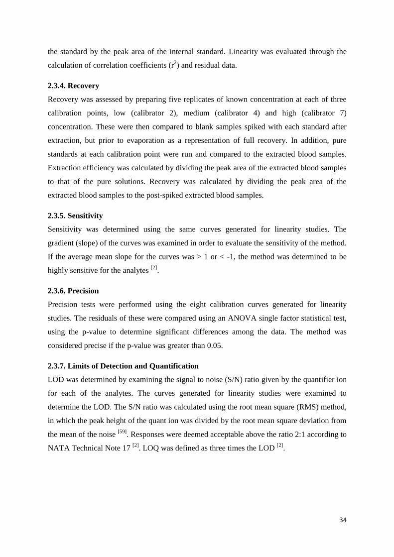
34

the standard by the peak area of the internal standard. Linearity was evaluated through the

calculation of correlation coefficients (r2) and residual data.

2.3.4. Recovery

Recovery was assessed by preparing five replicates of known concentration at each of three

calibration points, low (calibrator 2), medium (calibrator 4) and high (calibrator 7)

concentration. These were then compared to blank samples spiked with each standard after

extraction, but prior to evaporation as a representation of full recovery. In addition, pure

standards at each calibration point were run and compared to the extracted blood samples.

Extraction efficiency was calculated by dividing the peak area of the extracted blood samples

to that of the pure solutions. Recovery was calculated by dividing the peak area of the

extracted blood samples to the post-spiked extracted blood samples.

2.3.5. Sensitivity

Sensitivity was determined using the same curves generated for linearity studies. The

gradient (slope) of the curves was examined in order to evaluate the sensitivity of the method.

If the average mean slope for the curves was > 1 or < -1, the method was determined to be

highly sensitive for the analytes [2]

.

2.3.6. Precision

Precision tests were performed using the eight calibration curves generated for linearity

studies. The residuals of these were compared using an ANOVA single factor statistical test,

using the p-value to determine significant differences among the data. The method was

considered precise if the p-value was greater than 0.05.

2.3.7. Limits of Detection and Quantification

LOD was determined by examining the signal to noise (S/N) ratio given by the quantifier ion

for each of the analytes. The curves generated for linearity studies were examined to

determine the LOD. The S/N ratio was calculated using the root mean square (RMS) method,

in which the peak height of the quant ion was divided by the root mean square deviation from

the mean of the noise [59]

. Responses were deemed acceptable above the ratio 2:1 according to

NATA Technical Note 17 [2]

. LOQ was defined as three times the LOD [2]

.

35

3. Results and Discussion

3.1. Method Development

3.1.1. Characterisation

Characterisation was attempted using both ESI- and ESI+ mode. ESI+ mode was first trialled

due to this being the ionisation mode of choice for amatoxins in most of the literature

[1,9,11,39,41]. Much of the amatoxin literature used the m/z transitions from 919 → 901 and 920

→ 902 for α-amanitin and β-amanitin respectively [1,5,9,11,39]

. These transitions correlate to a

loss of water from the parent ions. In the majority of the literature this was the only transition

reported, and Nomura et al. [1]

could not achieve fragmentation at all. This suggests the parent

ions of the amanitins are difficult to fragment. The other most commonly reported daughter

ion for the amanitins was m/z 259. It was hypothesised that this ion is the fragment shown in

Figure 3.1 [43]

. This ion was thought to be more specific for the amatoxins than loss of water.

In addition, cone voltages and collision energies reported in the literature were no greater

than 50 V. It was hence hypothesised that increasing these values would increase the

fragmentation of the amatoxins and phallotoxins.

Figure 3.1. Possible fragment for m/z 259. [43]

Characterisation was performed using the automated IntelliStart system embedded in the

UPLC system software. It was thought that using this system, more unique transitions would

be observed and optimal conditions presented. However, ESI+ mode provided inconsistent

transitions at various concentrations. For α-amanitin, only one daughter ion was detected

using ESI+ mode (m/z 86.06), and this ion was considered unstable based on the

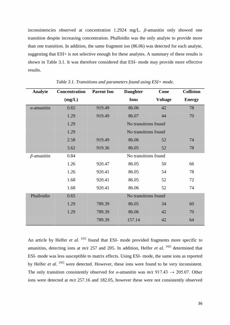
36

inconsistencies observed at concentration 1.2924 mg/L. β-amanitin only showed one

transition despite increasing concentration. Phalloidin was the only analyte to provide more

than one transition. In addition, the same fragment ion (86.06) was detected for each analyte,

suggesting that ESI+ is not selective enough for these analytes. A summary of these results is

shown in Table 3.1. It was therefore considered that ESI- mode may provide more effective

results.

Table 3.1. Transitions and parameters found using ESI+ mode.

Analyte Concentration

(mg/L)

Parent Ion Daughter

Ions

Cone

Voltage

Collision

Energy

α-amanitin 0.65 919.49 86.06 42 78

1.29 919.49 86.07 44 70

1.29 No transitions found

1.29 No transitions found

2.58 919.49 86.06 52 74

3.62 919.36 86.05 52 78

β-amanitin 0.84 No transitions found

1.26 920.47 86.05 50 66

1.26 920.41 86.05 54 78

1.68 920.41 86.05 52 72

1.68 920.41 86.06 52 74

Phalloidin 0.65 No transitions found

1.29 789.39 86.05 34 60

1.29 789.39 86.06 42 70

789.39 157.14 42 64

An article by Helfer et al. [42]

found that ESI- mode provided fragments more specific to

amanitins, detecting ions at m/z 257 and 205. In addition, Helfer et al. [42]

determined that

ESI- mode was less susceptible to matrix effects. Using ESI- mode, the same ions as reported

by Helfer et al. [42]

were detected. However, these ions were found to be very inconsistent.

The only transition consistently observed for α-amanitin was m/z 917.43 → 205.07. Other

ions were detected at m/z 257.16 and 182.05, however these were not consistently observed

37

with each characterisation attempt. The cone voltages and collision energies were also found

to vary. The results of characterisation using ESI- mode are shown in Table 3.2.

Table 3.2. Transitions and parameters found using ESI- mode.

Analyte Concentration

(mg/L)

Parent Ion Daughter

Ions

Cone

Voltage

Collision

Energy

α-amanitin 3.33 917.43 205.08 52 80

257.16 52 60

3.33 917.43 205.07 56 60

3.62 917.36 205.07 46 70

4.16 917.49 205.07 50 60

257.04 50 58

4.52 917.43 205.07 52 62

5.43 917.43 205.07 50 76

182.05 50 56

β-amanitin 2.10 918.41 205.07 64 62

3.36 918.47 205.07 60 46

188.04 60 60

3.36 918.41 205.07 60 66

257.11 60 58

3.76 918.41 205.07 60 72

257.11 60 64

187.98 60 66

3.76 918.47 205.14 52 70

188.04 52 78

257.13 52 68

3.76 918.47 205.14 58 68

187.97 58 66

257.17 58 48

Phalloidin 1.29 No transitions found

2.59 787.39 124.95 64 66

144.13 64 58

38

Despite increasing the concentration significantly for α-amanitin, the presence of the ions at

m/z 257 and 182 were highly inconsistent. This suggests that these fragments are not

reproducible. However, β-amanitin was shown to ionise far more consistently using ESI-

mode, showing three stable transitions upon increasing the concentration. Given this, and that

three transitions were observed for α-amanitin using ESI- mode compared to only one

transition using ESI+ mode, ESI- mode was chosen for use in the majority of the method

development stage.

In later stages, however, it was realised that sensitivity of the ions was significantly poorer

using ESI- mode. An article by Chung et al. [39]

also reported a decrease in sensitivity with

ESI- mode, and additionally found ESI- mode gave ions that were less stable than those

observed with ESI+ mode. ESI+ mode was therefore revisited. Upon increasing the

concentration of each analyte, the following transitions were observed (Table 3.3).

Table 3.3. Transitions and parameters found using ESI+ mode upon increasing

concentration of analytes.

Standard Concentration

(mg/L)

Parent

ion

Daughter

ions

Cone voltage

(V)

Collision energy

(V)

α-amanitin 9.681 919.30 86.12 52 80

259.18 52 52

143.15 52 66

β-amanitin 4.194 920.28 86.05 46 76

259.11 46 52

143.09 46 60

Phalloidin 2.585 789.26 86.06 44 78

157.08 44 62

173.99 44 66

Virginiamycin

B

2.042 867.35 134.06 52 48

205.08 52 56

177.11 52 76

Rifampicin 1.939 823.36 791.35 36 18

151.10 36 36

95.03 36 72

39

While the concentration had to be increased significantly in order to detect these transitions,

higher sensitivity was achieved when compared to ESI- mode (Table 3.4).

Table 3.4. Comparison of peak height of quantifier ion at 25 ng/mL within standard mix

using ESI+ and ESI- mode.

Standard ESI+ ESI-

α-amanitin 396 5

β-amanitin 370 3

Phalloidin 917 37

Virginiamycin B 5367 25

Rifampicin 11284 738

Given the significant increase in sensitivity, ESI+ mode was chosen as the ideal ionisation

method for this study.

3.1.2. Choice of Mobile Phases

Initial analysis proved that separation of the two amanitins was a difficult task. This is due to

their chemical similarity. Various parameters were adjusted in an effort to separate these

amanitins. Four different mobile phase combinations were trialled. The parameters evaluated

include flow rate, mobile phase composition and isocratic holds. Flow rates ranged between

0.2-0.5 mL/min, isocratic holds ranged from 15 seconds to 2 minutes, and initial mobile

phase composition ranged from 99% A/1% B to 70% A/30% B. Table 3.5 summarises the

optimised parameters for each mobile phase combination trialled.

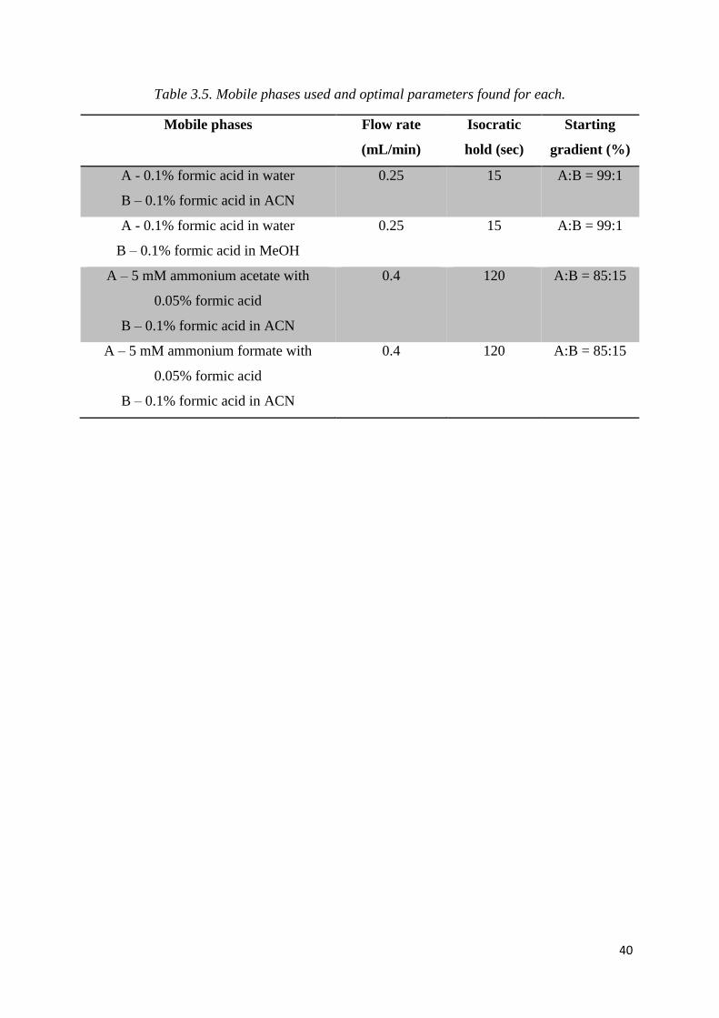
40

Table 3.5. Mobile phases used and optimal parameters found for each.

Mobile phases Flow rate

(mL/min)

Isocratic

hold (sec)

Starting

gradient (%)

A - 0.1% formic acid in water

B – 0.1% formic acid in ACN

0.25 15 A:B = 99:1

A - 0.1% formic acid in water

B – 0.1% formic acid in MeOH

0.25 15 A:B = 99:1

A – 5 mM ammonium acetate with

0.05% formic acid

B – 0.1% formic acid in ACN

0.4 120 A:B = 85:15

A – 5 mM ammonium formate with

0.05% formic acid

B – 0.1% formic acid in ACN

0.4 120 A:B = 85:15

41

Figure 3.2 below shows the resulting separation from each of these mobile phase

combinations under their optimal conditions.

Figure 3.2. Separation of α-amanitin and β-amanitin using a) 0.1% formic acid in water :

0.1% formic acid in acetonitrile, b) 0.1% formic acid in water : 0.1% formic acid in

methanol, c) 5 mM ammonium acetate with 0.05% formic acid : 0.1% formic acid in

acetonitrile (left peak = β-amanitin, right peak = α-amanitin). Note: secondary peak

observed in c) and d) for β-amanitin is a result of crossover between the two amanitins within

the mixture; this is not observed in individual samples under the same conditions.

The first mobile phase combination, 0.1% formic acid in water : 0.1% formic acid in

acetonitrile, showed minimal separation. The amatoxin literature was reviewed in an attempt

to find the most successful mobile phase combination. Much of the amatoxin literature used

methanol as mobile phase B. Therefore a mobile phase combination of 0.1% formic acid in

water : 0.1% formic acid in methanol was trialled. The best resolution between α-amanitin

and β-amanitin achieved while using methanol was less than that when acetonitrile was used.

42

The other common mobile phase encountered in the amatoxin literature was ammonium

acetate as the aqueous phase. This, in conjunction with 0.1% formic acid in acetonitrile as the

organic phase, was hence trialled. Results improved significantly with the use of this solvent,

and far greater separation was achieved. Given the improvement generated from ammonium

acetate, ammonium formate was also explored as ammonium formate was more readily

available in the laboratory. Ammonium formate gave a similar level of separation to

ammonium acetate, thus it was chosen as the aqueous mobile phase.

3.1.3. Choice of Column

In addition to the mobile phases, UPLC columns also had to be selected in order to optimise

separation of the amanitins. Four different columns were trialled in this study. Table 3.6

summarises the optimised parameters for each column trialled, and Figure 3.3 shows the

resulting chromatograms.

Table 3.6. Columns used and optimal parameters found for each.

Column Mobile Phases Flow rate

(mL/min)

Isocratic

hold (sec)

Starting

gradient (%)

Waters ACQUITY

UPLC BEH Phenyl

10 cm

A - 0.1% formic acid in water

B – 0.1% formic acid in ACN

0.25 15 A:B = 99:1

Waters ACQUITY

UPLC BEH C18

5 cm

A - 0.1% formic acid in water

B – 0.1% formic acid in ACN

0.25 15 A:B = 99:1

Grace Vision HT

C18 Basic 3 µm

A – 5 mM ammonium acetate

with 0.05% formic acid

B – 0.1% formic acid in ACN

0.25 None A:B = 95:5

Waters ACQUITY

UPLC BEH C18

15 cm

A – 5 mM ammonium acetate

with 0.05% formic acid

B – 0.1% formic acid in ACN

0.4 120 A:B = 85:15

43

Figure 3.3. Separation of α-amanitin and β-amanitin using a) 10 cm Phenyl column, b) 5 cm

C18 column, c) 15 cm HPLC column and d) 15 cm UPLC C18 column (left peak = β-

amanitin, right peak = α-amanitin)

The Waters ACQUITY UPLC BEH Phenyl 10 cm column showed some level of separation,

but baseline separation could not be achieved. The Waters ACQUITY UPLC BEH C18 5 cm

column was even less effective, despite much of the literature recommending the use of a

C18 column. A 15 cm Grace Vision HT C18 column was then trialled in the hopes that the

longer column length would give greater separation. This showed better resolution of the two

amanitins than the previous columns. However, this column is designed for HPLC and is

unable to reach the high pressures used in UPLC. In addition, particles within HPLC columns

are larger than those of UPLC columns, reducing the interaction between the analyte and the

column. Therefore a 15 cm Waters ACQUITY UPLC BEH C18 column was trialled, and

baseline separation was finally achieved. The extra length of the column allows more

interaction between the analyte and the particles within the column. This hence produced

greater separation and better resolution of the peaks.

44

3.1.4. Choice of Gradient System

The amanitins eluted first in every gradient method trialled, usually within the first 2 minutes.

Gradients at which each toxin eluted were determined from retention times over several

injections by calculating the mobile phase composition at which the toxins eluted. It was

calculated that the amanitins were eluting when the gradient was at approximately 85% A :

15% B. Therefore an isocratic hold of 2 minutes at this gradient was utilised to better separate

the amanitins.

The next compound to elute was phalloidin. This eluted after approximately 3 minutes. It was

calculated that phalloidin was eluting at a gradient of approximately 40% A : 60% B.

Therefore the gradient was ramped to 40% A : 60% B between 2-4 minutes.

Finally, the internal standards eluted between 4-5 minutes, and it was calculated that these

were eluting at a gradient of approximately 10% A : 90% B. Therefore between 4-6 minutes

the gradient was ramped to 10% A : 90% B. The final gradient program is shown in Figure

3.4.

Figure 3.4. Gradient program developed for amatoxin and phallotoxin analysis.

α-amanitin RT =

1.75

β-amanitin RT =

1.65

Phalloidin

RT = 3.56

Rifampicin

RT = 4.96

0

10

20

30

40

50

60

70

80

90

100

0 1 2 3 4 5 6 7 8

Mobile Phase (%)

Time (min)

Gradient Program

↓ ↓

↓

↓

↓

Virginiamycin B

RT = 5.19

45

3.1.5. Choice of Reconstitution Solvent

In early stages of this study, a second peak was observed for α-amanitin when the analyte was

reconstituted in a strong solvent. Pure solutions were initially reconstituted in 50 µL

acetonitrile, and later 50 µL methanol. In both instances a second peak was observed for α-

amanitin. More dilute solvents were trialled, with 50% acetonitrile or methanol in water

being investigated as a reconstitution solvent. In both cases this significantly diminished the

presence of the secondary peak. Each solvent was further diluted to 10% acetonitrile or

methanol in water, which eliminated the secondary peak completely. Figure 3.5 below shows

the progressive elimination of this peak through dilution. It is uncertain what this peak was,

but it is suspected that there was an impurity within the sample which was water soluble and

therefore not detected when a highly aqueous reconstitution solvent was used. Alternatively,

it could be the result of an issue with chromatography caused by the amount of organic

solvent present.

46

Figure 3.5. Investigation of reconstitution solvent using a) 100% acetonitrile, b) 100%

methanol, c) 50% acetonitrile in water, d) 50% methanol in water, e) 10% acetonitrile in

water and f) 10% methanol in water.

Initially, 10% acetonitrile in water was chosen as the reconstitution solvent as it gave slightly

better peak shape than 10% methanol in water. In later stages of this study, once the mobile

phase was adapted to 5 mM ammonium formate with 0.05% formic acid : 0.1% formic acid

47

in acetonitrile, it was found that reconstituting in this mobile phase gave greater sensitivity.

This was further investigated through the development of the sample preparation method.

3.1.6. Sample Preparation

Sample preparation steps prior to extraction were explored. In the majority of the literature, a

simple dilution step was used prior to extraction using SPE [1,9,11,41,42]

. One article by

Filigenzi et al. [15]

utilised protein precipitation, so this method was trialled. LLE is also a

common and simple extraction method, and while not used in the literature was trialled for

this study.

3.1.6.1. Protein Precipitation

Protein precipitation was performed prior to SPE. Extraction was then carried out using the

methods outlined by both Nomura et al. [1]

and Filigenzi et al. [15]

. However, both these

methods proved unsuccessful as none of the analytes were detected in the final extract. It is

suspected that the amatoxins were settling with the proteins rather than being extracted into

the supernatant. This is potentially due to their large size, or formation of emulsions causing

issues with adsorption and bonding. This method was therefore not pursued further.

3.1.6.2. Liquid-Liquid Extraction

LLE was also performed as this was considered a much faster and simpler method than SPE.

However, as with protein precipitation, the amanitins could not be detected after LLE and

therefore the method was not pursued further.

3.1.6.3. Dilution

Dilution was performed in the same manner as the method reported by Nomura et al. [1]

.

Dilution was considered a simple step, and necessary as whole blood is a complex matrix

with many potential interferents. Direct injection of whole blood onto the UPLC-MS/MS

would result in clogging of the instrument with unwanted components and instrument failure.

The analytes were able to be detected after extraction of diluted samples. This method was

hence carried through the rest of the experimental process.

3.1.6.4. Solid Phase Extraction

The majority of the literature studying amanitins utilised Oasis HLB cartridges (60 mg).

Seven different SPE sorbents were trialled in this study. These included the Oasis HLB

(reverse-phase), Oasis MCX (mixed mode cation exchange), UCT Clean Screen DAU (mixed

mode cation exchange), UCT Styre Screen BCX (mixed mode), UCT Clean Screen XCEL

48

(mixed mode), UCT Clean Up C18 (hydrophobic interaction) and Agilent Bond Elut Plexa

PCX (cation exchange). Each of these was initially trialled using the extraction method

outlined by Nomura et al. [1]

, reconstituting the sample in 100 µL of 10% acetonitrile in water

and filtering with a 0.2 µm syringe filter. Extraction efficiencies were calculated by

comparing the extracted samples with pure solutions at the same concentration. Extraction

efficiencies were all very low for both amanitins, as shown in Table 3.7.

49

Table 3.7. Extraction efficiencies of standards at 75 ng/mL (ESI- mode).

Standard Oasis HLB Oasis MCX UCT Clean

Screen

UCT Clean

Screen XCEL

UCT Styre Screen UCT Clean Up Agilent Bond

Elut Plexa

α-amanitin 11 - 46 30 4 22 -

β-amanitin 12 - 13 64 9 27 -

Phalloidin 40 - 97 104 52 71 -

Virginiamycin B 182 - 371 408 313 101 -

Rifampicin 90 - 192 188 123 105 -

50

While extraction efficiencies were low for the amanitins, the internal standards show very

high extraction efficiencies. Virginiamycin B in particular shows unusually high results, and

it is uncertain whether these are true results. This was further investigated in later stages of

the study.

The results in Table 3.7 were generated using ESI- mode. When the method was adapted in

later stages for ESI+ mode, these extractions were trialled again to see if results improved.

Only three columns were evaluated at this stage, Oasis HLB, UCT Clean Screen XCEL and

UCT Clean Up, as these were the most effective columns (Table 3.8). The UCT Clean Screen

columns also presented good extraction efficiencies, however there were no more available at

this stage and so these were not evaluated.

Table 3.8. Extraction efficiencies of standards at 200 ng/mL (ESI+ mode).

Standard Oasis HLB UCT Clean Screen XCEL UCT Clean Up

α-amanitin 56 59 88

β-amanitin 3 23 109

Phalloidin 22 33 29

Virginiamycin B 493 3089 334

Rifampicin 282 151 95

Again, the internal standards present unusually high extraction efficiencies. However,

extraction efficiencies for the amanitins have drastically improved. This suggests that there

was ion suppression occurring using ESI- mode. The greatest extraction efficiencies were

obtained with the UCT Clean Up columns. The C18 functionality of this column appears to

be the most appropriate for these analytes. This column was hence used for all further

analysis.

In addition to the column, other considerations for SPE include the solvents used for the

conditioning, washing and eluting steps. The initial concentration range trialled was from 5-

500 ng/mL. The method by Nomura et al. [1]

was able to detect the amanitins, however

extraction efficiencies were relatively low at lower concentrations. This was due to poor

reproducibility of the method at these lower concentrations. The method was hence altered in

various ways according to other methods reported in the literature to determine which had the

greatest effect on sensitivity and extraction efficiency. In addition, the method by Filigenzi et

51

al. [15]

was explored as this method was the only one found to use the UCT Clean Up

columns. These are summarised in Table 3.9, and peak areas generated from these methods

are shown in Table 3.10.

52

Table 3.9. Methods and variations trialled for SPE.

SPE Steps Original

Method

Method 1 Method 2 Method 3 Method 4 Method 5 Filigenzi et al. [15]

Conditioning

step

2 mL MeOH

and 2 mL

water

2 mL MeOH, 2 mL

water and 2 mL

phosphate buffer

2 mL MeOH

and 2 mL

water

2 mL MeOH

and 2 mL

water

2 mL MeOH

and 2 mL

water

2 mL MeOH

and 2 mL

water

3 mL MeOH, 3 mL

water and 3 mL

phosphate buffer

Wash step 2 mL water 2 mL water 5 mL water 2 mL water 2 mL water 2 mL 5%

MeOH in

water

5 mL water, 3 mL 0.1

M acetic acid and 5 mL

DCM/MeOH (95:5)

Elution step 3 mL MeOH 3 mL MeOH 3 mL MeOH 6 mL MeOH 3 mL MeOH 3 mL MeOH 4 mL MeOH

Reconstitution

step

100 µL 10%

ACN in

water

100 µL 10% ACN

in water

100 µL 10%

ACN in

water

100 µL 10%

ACN in

water

250 µL 10%

ACN in

ammonium

formate

buffer

100 µL 10%

ACN in water

250 µL 10% ACN in

ammonium formate

buffer

53

Table 3.10. Differences in peak area resulting from various extraction methods.

Standard Original

Method

Method

1

Method

2

Method

3

Method

4

Method

5

Filigenzi

et al. [15]

α-amanitin 61 88 107 26 133 116 -

β-amanitin 57 76 66 31 85 58 -

Phalloidin 106 93 113 86 131 93 -

Virginiamycin

B

3709 2261 3479 2849 7243 3838 -

Rifampicin 1084 321 298 277 1103 1038 -

Based on the above data (Tables 3.9 and 3.10), it was determined that adding 5% methanol to

the wash step and reconstituting in 10% acetonitrile in ammonium formate gave the most

improvement. It was then considered that sensitivity could be further improved if the

composition of the reconstitution solvent was adapted to match the initial gradient of the

method. A composition of 85% A : 15% B was then trialled, as well as compositions of 80%

A : 20% B and 75% A : 25% B for comparison. The greatest sensitivity was achieved when

the reconstitution solvent was at a mobile phase composition of 80% A : 20% B. These

adaptations were hence made to the original extraction method to form the final developed

method for this study.

In an attempt to further increase sensitivity of the analytes, the post-extraction steps were also

evaluated. The extracts produced from the method were determined to be relatively clear, and

as a result it was considered that the syringe filtering step was unnecessary. It was also

suspected that the analytes were not passing through the filter, which could account for the

low sensitivity. Two pure solutions were prepared, with one being reconstituted in 50 µL

mobile phase (80% A : 20% B) and the other reconstituted in 75 µL mobile phase (80% A :

20% B) before being filtered. The sample to be filtered was reconstituted in 75 µL as too

little extract was recovered from filtering 50 µL, making analysis difficult. The results of this

are presented in Table 3.11 below.

54

Table 3.11. Comparison of peak area for quantifier ion using 100 ng/mL pure solutions with

and without filtering step.

Analyte No filter Filter

Concentration

(ng/mL)

Peak Area Concentration

(ng/mL)

Peak Area Expected

Peak Area

α-amanitin 100 1367 66.67 95 911

β-amanitin 100 836 66.67 61 557

Phalloidin 100 661 66.67 38 441

As seen in Table 3.11, the amount of analyte detected was significantly decreased in the

filtered samples, producing a loss of approximately 90% for each analyte. The filtering step

was hence removed from the method.

3.1.7. Choice of Internal Standard

Many different internal standards were evaluated for use in amatoxin analysis throughout the

literature. Internal standards used in the literature include microcystin RR, γ-amanitin methyl

ether, tilmicosin and virginiamycin B [1, 3, 7, 14, 17, 20]

. Nomura et al. [1]

chose to use

virginiamycin B as it gave the highest recovery values, making it the most effective internal

standard. As such, virginiamycin B was included as part of the whole blood analysis. In

addition, although not chosen for the final analysis, other studies evaluated the use of

rifampicin as an internal standard [1, 3, 21]

. Rifampicin was hence included in this study.

It had been previously observed earlier in this study that extraction efficiencies for

virginiamycin B were abnormally high. Rifampicin was therefore compared with

virginiamycin B by analysing two standard mixtures each with one of the internal standards

added, in order to determine the best choice for whole blood analysis according to the

optimised method. The results are shown in Table 3.12.

55

Table 3.12. Comparison of internal standards within a 25 ng/mL mixture.

Internal

Standard

Peak Area

α-amanitin β-amanitin Phalloidin Virginiamycin B Rifampicin

Virginiamycin B 124 101 451 19237 -

Rifampicin 233 153 560 - 9051

A noticeable reduction of the amanitins and phalloidin was observed in the sample containing

virginiamycin B. This suggests that virginiamycin B is reacting with the amanitins in a way

that reduces their sensitivity, although the reason for this is not known. Rifampicin was hence

chosen as the internal standard for all future stages of this study.

3.2. Validation

Validation of a method is an essential process as it ensures that a method is “fit for purpose”

and can produce results which are reliable and reproducible [2]

. For this study, validation was

carried out following guidelines outlined in NATA Technical Note 17 [2]

and Shah et al. [3]

.

The validation parameters investigated in this study included selectivity, matrix effects,

linearity, recovery, sensitivity, precision and limits of detection and quantification.

3.2.1. Selectivity

Selectivity aims to determine potential interferents that may hinder the detection of an analyte

[2]. If a method can distinguish a particular analyte from other analytes, the method is said to

be selective for these analytes [2]

. For this study, eight drug mixtures containing various drugs

were analysed using the developed method in order to determine whether any interference

would be detected within the windows allocated for amanitins. Some examples of drugs

examined include ibuprofen, pseudoephedrine, caffeine, codeine, morphine, cocaine,

ketamine, MDMA, THC, cathinones and amphetamines (see Appendix 1 for full list). These

drugs are not chemically similar to the amanitins, however were considered useful as they are

commonly encountered in toxicological analyses.

No interference was observed in any of the detection windows for each of the amanitins or

phalloidin, hence none of the drugs within these mixtures were determined to be an

interferent for these analytes. As such, the developed method is considered a highly selective

method for amanitins.

56

3.2.2. Matrix effects

Matrix effects are caused when interferents within the matrix alter the results given by the

analyte [2]

. In this study, matrix effects were evaluated in a similar manner to selectivity.

Blank blood samples, including an artificially putrefied blood sample and a blood from

muscle sample, were extracted and analysed using the developed method, with the detection

windows of the amanitins and phalloidin being investigated for signs of any interference.

No significant interference was observed in the detection windows for the amanitins,

however multiple peaks and a poor baseline were observed in the detection window for

phalloidin. The effect of the matrix on the analytes was then calculated by dividing the peak

area of a post-spiked extract by the peak area of a pure solution, and calculating the

percentage. This was done at each of three calibration points, low (calibrator 2), medium

(calibrator 4) and high (calibrator 7) concentration. If the percentage was greater than 100%,

this was indicative of ion enhancement. If the percentage was lower than 100%, this was

indicative of ion suppression. The average calculated matrix effects for α-amanitin, β-

amanitin and phalloidin were 149%, 280% and 147% respectively. This indicates significant

ion enhancement of the analytes. The extraction method hence needs to be further optimised

to resolve these issues.

3.2.3. Linearity

Linearity tests measure the proportionality of an analyte’s response over a specified

concentration range [2]

. To determine the concentration range at which spiked samples should

be measured, pure solutions containing each of the analytes were prepared at a range of 5-500

ng/mL. Upon visual examination of the results, it was determined that the amanitins could not

be observed below 25 ng/mL with a degree of certainty, however phalloidin could be

observed as low as 5 ng/mL. Calibration standards were hence prepared at a range of 25-500

ng/mL for α-amanitin and β-amanitin, and at a range of 5-100 ng/mL for phalloidin.

Four sets of calibrators were prepared for linearity tests, with each set being injected twice.

Since seven calibration points were chosen and only six are necessary according to the

NATA guidelines [2]

, this allowed elimination of observed outliers. Individual curves were

inspected for outliers by using the generated equation to calculate expected concentrations

from the response ratio. A point was considered an outlier if the difference between expected

concentration and actual concentration was greater than 20%, and hence removed from

57

further calculation steps (see Appendix 2). The average response ratios were then plotted to

determine if a linear relationship was observed (Figure 3.6).

58

Figure 3.6. Linearity plots for α-amanitin, β-amanitin and phalloidin.

y = 0.0031x - 0.0391 R² = 0.9731

0

0.2

0.4

0.6

0.8

1

1.2

1.4

1.6

1.8

0 100 200 300 400 500 600

Response Ratio

Concentration (ng/mL)

Alpha-Amanitin Average Linear Plot

y = 0.0022x - 0.0231 R² = 0.9825

0

0.2

0.4

0.6

0.8

1

1.2

0 100 200 300 400 500 600

Response Ratio

Concentration (ng/mL)

Beta-Amanitin Average Linear Plot

y = 0.0002x - 0.0002 R² = 0.9872

0

0.01

0.02

0.03

0.04

0.05

0.06

0.07

0.08

0.09

0.1

0 100 200 300 400 500 600

Response Ratio

Concentration (ng/mL)

Phalloidin Average Linear Plot

59

As can be seen in Figure 3.6, there is some evidence of a linear relationship. The average

correlation coefficients (r2) for α-amanitin, β-amanitin and phalloidin are 0.9731, 0.9825 and

0.9872 respectively. ACTGAL standards require that r2 ≥ 0.997, or r

2 ≥ 0.98 for non-critical

methods. This suggests that, while not optimal, this method is sufficiently linear for the

analytes. However, it is important not to use the r2 value as the sole measure of a linear

relationship as it must also be demonstrated that the data is evenly distributed [60]

. This was

assessed through residual plots.

Residual plots are used to determine if there is any significant difference between data points.

If the variance between data points is evenly distributed, this shows goodness of fit [60]

. If the

variance is not evenly distributed, or there is evidence of a trend in the data, then the data

may not demonstrate a normal distribution [60]

. Residual data in shown in Figure 3.7.

60

Figure 3.7. Residual plots for α-amanitin, β-amanitin and phalloidin.

-0.6

-0.4

-0.2

0

0.2

0.4

0.6

0.8

1

1.2

0 100 200 300 400 500 600

Residual

Concentration (ng/mL)

Alpha-Amanitin Residual Plot

Curve 1

Curve 2

Curve 3

Curve 4

Curve 5

Curve 6

Curve 7

Curve 8

-0.4

-0.2

0

0.2

0.4

0.6

0.8

0 100 200 300 400 500 600

Residual

Concentration (ng/mL)

Beta-Amanitin Residual Plot

Curve 1

Curve 2

Curve 3

Curve 4

Curve 5

Curve 6

Curve 7

Curve 8

-0.06

-0.04

-0.02

0

0.02

0.04

0.06

0.08

0 100 200 300 400 500 600

Residual

Concentration (ng/mL)

Phalloidin Residual Plot

Curve 1

Curve 2

Curve 3

Curve 4

Curve 5

Curve 6

Curve 7

Curve 8

61

There is an apparent trend in the residual plots, with each analyte showing an increase in

variance as the concentration is increased. This indicates the data points may not exhibit

normal distribution. An ANOVA single factor test was therefore applied to the data to test for

any significant difference. Data was determined to be significantly different if the F statistic

given for the data exceeded the F critical value. For the amanitins, the F critical was

calculated to be 2.318, and for phalloidin was 2.330. The F statistics for α-amanitin, β-

amanitin and phalloidin were calculated to be 1.016, 0.603 and 0.531 respectively (see

Appendix 3 for full data). For each analyte, the F statistic was well below the F critical value.

This means that there was no significant difference found in the data. Therefore there is

evidence of a linear relationship that is normally distributed.

3.2.4. Recovery

After discovering that phalloidin, despite showing high sensitivity in the pure solutions, was

not well detected at the lower calibrators, recovery studies were performed. Recovery testing

determines the amount of analyte able to be detected from a biological specimen after the

extraction process [2]

. Recovery was conducted using the method outlined in Shah et al. [3]

.

Five replicates of low (calibrator 2), medium (calibrator 4) and high (calibrator 7)

concentration were analysed. These were compared to pure solutions to calculate extraction

efficiency, and compared to blank blood extracts spiked with each analyte post-extraction but

pre-evaporation to calculate recovery. Extraction efficiencies greater than 100% were

indicative of ion enhancement, and those lower than 100% were indicative of ion

suppression. Recoveries above 50% were considered acceptable. Extraction efficiency and

recovery data are shown in Table 3.14 below.

62

Table 3.13. Average extraction efficiency and recovery values for α-amanitin, β-amanitin and

phalloidin.

Calibration Point Standard Average Extraction

Efficiency (%)

Average Recovery

(%)

Cal 2 α-amanitin 164 100

β-amanitin 196 47

Phalloidin 18 9

Cal 4 α-amanitin 142 79

β-amanitin 143 53

Phalloidin 11 7

Cal 7 α-amanitin 152 108

β-amanitin 158 62

Phalloidin 9 12

Extraction efficiencies for both amanitins are very high. Recoveries for α-amanitin are also

very high. For β-amanitin, recoveries are acceptable for the medium and high calibration

points, but are below 50% at calibrator 2. This could indicate poor reproducibility at lower

concentrations. Phalloidin shows very poor extraction efficiency and recovery, suggesting the

extraction method is not effective for phalloidin. Overall, the extraction method developed in

this study is effective for both the amanitins, but the method would have to be further

optimised in order to improve the recovery of phalloidin.

3.2.5. Sensitivity

Sensitivity determines the rate at which a measured response changes with a change in

concentration of an analyte [2]

. Sensitivity is evaluated by examining the gradient, or slope, of

a calibration curve. If the mean gradient of a curve or set of curves is > 1 or < -1, this is an

indication of high sensitivity [2]

.

In this study, sensitivity was determined using the results generated from the linearity curves

(Figure 3.5). The mean slope resulting from each of the eight curves was 0.0031, 0.0022 and

0.0002 for α-amanitin, β-amanitin and phalloidin respectively. This suggests that the

developed method is not highly sensitive for these analytes.

63

3.2.6. Precision

Precision measures the variation between independent replicates of the same sample [2]

.

Precision was assessed through the use of an ANOVA single factor statistical test. This was

performed using the residual data generated from the eight curves used in linearity studies. If

the p-value generated from the residual data was greater than 0.05, results were deemed not

significantly different from each other and the method was considered precise.

The p-values calculated for α-amanitin, β-amanitin and phalloidin were 0.4279, 0.7265 and

0.7814 respectively (see Appendix 3 for full data). This means that among the individual

samples for each standard, no significant difference among the data was observed. Therefore

the method is precise for each of the standards.

Accuracy was also considered for this study, however given that the purchased amanitins and

phalloidin were not of 100% purity, this was not able to be evaluated. It was not possible to

buy pure standards for the amanitins or phalloidin. The only standards that could be obtained

were of less than 100% purity, and these standards were very expensive which further limited

possible validation steps. Accuracy was investigated in other literature for amanitins despite

the standards not being 100% pure, and in none of these articles was the actual purity

accounted for. These results hence do not represent true accuracy. It was determined that any

accuracy results produced from this study would also not be representative of the actual

accuracy of the method, and so this step was not included in this study.

3.2.7. Limits of Detection and Quantification

The limit of detection (LOD) gives an indication of the lowest concentration at which it can

be determined that the analyte is present [2]

. There are various ways to evaluate this, however

the method chosen for this study was determination of the signal to noise (S/N) ratio.

According to the NATA guidelines [2]

, acceptable S/N ratios for LOD are either 2:1 or 3:1.

For this study, the ratio of 2:1 was chosen as an acceptable LOD.

For the amanitins, acceptable S/N ratios were found for the quantifier ions at levels as low as

25 ng/mL, and average RMS values for α-amanitin and β-amanitin were calculated at 7.29

and 4.81 respectively (see Appendix 4 for full data). However, phalloidin showed a

significant amount of noise compared to signal at the lower calibrators. While phalloidin

could easily be detected at 5 ng/mL in pure standards, the matrix effects generated by whole

blood severely impacted detection of phalloidin up to 20 ng/mL. The lowest concentration for

phalloidin at which an acceptable S/N ratio could be determined was 20 ng/mL, at which

64

point an average RMS value of 2.49 was calculated. LODs for α-amanitin and β-amanitin

were hence determined to be 25 ng/mL, and for phalloidin was 20 ng/mL.

The limit of quantitation (LOQ) indicates the lowest concentration at which a sample is able

to be reliably detected and quantified [2]

. According to the NATA guidelines [2]

, the LOQ can

be defined as three times the LOD. Therefore, the LOQs for the amanitins and phalloidin can

be calculated as 75 ng/mL and 60 ng/mL respectively.

65

4. Conclusions and Recommendations

4.1. Conclusions

A method was developed for the detection of α-amanitin, β-amanitin and phalloidin in whole

blood using UPLC-MS/MS. The increasing number of poisoning cases involving A.

phalloides in Australia has emphasised the need for a rapid method of detection of the toxins

within this mushroom. The method presented in an article by Nomura et al. [1]

, which

reported successful detection and quantification of these toxins in serum, plasma and urine,

provided the basis for the developed method. However, detection of the analytes using this

method could not be achieved. The method was therefore adapted by changing various

parameters in the ionisation, chromatography and sample preparation stages. The developed

method, while able to detect each of the analytes, presented various issues in the validation

stage of the study.

Mass spectrometry conditions were first optimised for each analyte. An electrospray interface

was used to detect transitions between parent and daughter ions. Both ESI+ and ESI- mode

were trialled, with ESI+ ultimately presenting more stable daughter ions at greater sensitivity.

UPLC conditions varied included the mobile phase combination, choice of column, flow rate

and isocratic holds. A mobile phase combination of 5 mM ammonium formate with 0.05%

formic acid : 0.1% formic acid in water at a flow rate of 0.4 mL/min gave optimal separation

of the analytes. Two internal standards, virginiamycin B and rifampicin, were trialled in this

study. Rifampicin was chosen as the internal standard as virginiamycin B was found to cause

a decrease in the sensitivity of the amanitins.

The developed method was then validated according to guidelines presented in NATA

Technical Note 17 [2]

and Shah et al. [3]

. Parameters assessed included selectivity, matrix

effects, linearity, recovery, sensitivity, precision and limits of detection and quantification.

The developed method proved to be selective for both the amanitins and phalloidin.

Significant matrix effects impacted the detection of phalloidin at lower concentrations,

making further results for phalloidin somewhat unreliable. In addition, ion enhancement was

observed for the analytes which impacted further results. Linearity studies showed normal

distribution of data with acceptable r2 values for each analyte, however these could be

improved. Recovery for the amanitins was acceptable, but poor recovery was observed for

phalloidin, suggesting the developed method is not ideal for phalloidin. Sensitivity was poor

for each of the analytes, indicating further optimisation of the developed method is required.

66

The method was found to be precise for each of the analytes. The LODs for α-amanitin, β-

amanitin and phalloidin were 25 ng/mL, 25 ng/mL and 20 ng/mL respectively. LOQs were

calculated as three times the LOD and hence were 75 ng/mL, 75 ng/mL and 60 ng/mL for α-

amanitin, β-amanitin and phalloidin respectively.

The developed method provides a good basis for detection of A. phalloides toxins, however

does not quite meet necessary standards. Despite this, the method offers significant potential

to achieving rapid and effective detection of amatoxins and phallotoxins in whole blood.

4.2. Recommendations

The method developed in this study should be revisited in order to increase sensitivity,

reliability and reproducibility. The sample preparation method in particular should be

optimised to improve recovery of β-amanitin and phalloidin, which should result in more

reliable detection. Different modes for MS/MS should also be investigated to improve

fragmentation of parent ions and possibly increase sensitivity.

Other technologies should also be investigated. Much of the literature utilised UPLC-TOF-

MS for detection of amatoxins in various matrices. This method should be evaluated for

detection of amatoxins and phallotoxins in whole blood. A number of other technologies

were reviewed in this study which could also provide potentially improved methods for

amatoxin detection.

Due to time restraints the second and third aims of the study, analysis of amatoxins in

putrefied blood and authentic specimens, were not attempted. These should both be

investigated in future work. Putrefied blood specimens would provide an insight into the

applicability of this method to post-mortem samples. Authentic specimens would also need to

be investigated to ensure the method’s effectiveness to real cases of A. phalloides poisoning.

This was ultimately the goal of this study, and although this was not achieved the developed

method offers a significant step forward in reaching this goal.

67

References:

1. Nomura M, Suzuki Y, Kaneko R, Ogawa T, Hattori H, Seno H, Ishii A. Simple and rapid

analysis of amatoxins using UPLC-MS-MS. Forensic Toxicology. 2012; 30(2):185-192.

2. National Association of Testing Authorities, Australia. Guidelines for the validation and

verification of quantitative and qualitative test methods; 2013. Technical Note 17.

3. Shah V, Midha K, Findlay J, Hill H, Hulse J, McGilveray I, McKay G, Miller K, Patnaik

R, Powell M, Tonelli A, Viswanathan C, Yakobi A. Bioanalytical method validation - A

revisit with a decade of progress. Pharmaceutical Research. 2000; 17(12):1551-1557.

4. Gonmori K, Yoshioka N. Mushroom toxins. In: Suzuki O, Watanabe K, editors. Drugs and

poisons in humans: A handbook of practical analysis. Berlin: Springer; 2005. 469-480.

5. Gonmori K, Fujita H, Yokoyama K, Watanabe K, Suzuki O. Mushroom toxins: A forensic

toxicological review. Forensic Toxicology. 2011; 29(2):85-94.

6. Blackman J. Clinical approach to toxic mushroom ingestion. Journal of the American

Board of Family Medicine. 1994; 7(1):31-37.

7. Trim G, Lepp H, Hall M, McKeown R, McCaughan G, Duggan G. Poisoning by Amanita

phalloides ("deathcap") mushrooms in the Australian Capital Territory. The Medical Journal

of Australia. 1999; 171(5):247-249.

8. Escudie L, Francoz C, Vinel J, Moucari R, Cournot M, Paradis V, Sauvanet A, Belghiti J,

Valla D, Bernuau J, Durand F. Amanita phalloides poisoning: Reassessment of prognostic

factors and indications for emergency liver transplantation. Journal of Hepatology. 2007;

46(3):466-473.

9. Tanahashi M, Kaneko R, Hirata Y, Hamajima M, Arinobu T, Ogawa T, Ishii A. Simple

analysis of α-amanitin and β-amanitin in human plasma by liquid chromatography-mass

spectrometry. Forensic Toxicology. 2010; 28(2):110-114.

10. Bidnychenko Y. Detecting mushroom peptide toxins in body fluids by capillary

electrophoresis. Liquid Chromatography Gas Chromatography. 2001; 19(9):1000-1002.

11. Leite M, Freitas A, Azul A, Barbosa J, Costa S, Ramos F. Development, optimisation and

application of an analytical methodology by ultra performance liquid chromatography-

tandem mass spectrometry for determination of amanitins in urine and liver samples.

Analytica Chimica Acta. 2013; 799(1):77-87.

12. Roberts D, Hall M, Falkland M, Strasser S, Buckley N. Amanita phalloides poisoning and

treatment with silibinin in the Australian Capital Territory and New South Wales. The

Medical Journal of Australia. 2013; 198(1):43-47.

13. Maurer H, Kraemer T, Ledvinka O, Schmitt C, Weber A. Gas chromatography-mass

spectrometry (GC-MS) and liquid chromatography-mass spectrometry (LC-MS) in

toxicological analysis: Studies on the detection of clobenzorex and its metabolites within a

68

systematic toxicological analysis procedure by GC-MS and by immunoassay and studies on

the detection of alpha- and beta-amanitin in urine by atmospheric pressure ionisation

electrospray LC-MS. Journal of Chromatography: Biomedical Sciences and Applications.

1997; 689(1):81-89.

14. Enjalbert F, Rapior S, Nouguier-Soule J, Guillon S, Amouroux N, Cabot C. Treatment of

amatoxin poisoning: 20 year retrospective analysis. Journal of Toxicology - Clinical

Toxicology. 2002; 40(6):715-757.

15. Filigenzi M, Poppenga R, Tiwary A, Puschner B. Determination of α-amanitin in serum

and liver by multistage linear ion trap mass spectrometry. Journal of Agricultural and Food

Chemistry. 2007; 55(8):2784-2790.

16. Mengs U, Pohl R, Mitchell T. Legalon ® SIL: the antidote of choice in patients with

acute hepatotoxicity from amatoxin poisoning. Current Pharmaceutical Biotechnology. 2012;

13(10):1964-1970.

17. Ahmed W, Gonmori K, Suzuki M, Watanabe K, Suzuki O. Simultaneous analysis of α-

amanitin, β-amanitin and phalloidin in toxic mushrooms by liquid chromatography coupled to

time-of-flight mass spectrometry. Forensic Toxicology. 2010; 28(2):69-76.

18. Wieland T, Gotzendorfer C, Zanotti G, Vaisius A. The effect of the chemical nature of

the side chains of amatoxins in the inhibition of eukaryotic RNA polymerase B. European

Journal of Biochemistry. 1981; 117(1):161-164.

19. Enjalbert F, Cassanas G, Salhi S, Guinchard C, Chaumont J. Distribution of the

amatoxins and phallotoxins in Amanita phalloides: Influence of the tissues and the collection

site. Rendered Accounts of the Academy of Sciences - Series III - Life Sciences. 1999;

322(10):855-862.

20. Vargas N, Bernal A, Sarria V, Franco-Molano A, Restrepo S. Amatoxin and phallotoxin

composition in species of the genus Amanita in Colombia: A taxonomic perspective.

Toxicon: Official Journal of the International Society on Toxinology. 2011; 58(6):583-590.

21. Wieland T. Poisonous principles of mushrooms of the genus Amanita. Science. 1968;

159(3818):946-952.

22. Lengsfeld A, Low I, Wieland T, Dancker P, Hasselbach W. Interaction of phalloidin with

actin. Proceedings of the National Academy of Sciences of the United States of America.

1974; 71(7):2803-2807.

23. Wieland T. The toxic peptides from Amanita mushrooms. International Journal of Peptide

and Protein Research. 1983; 22(3):257-276.

24. Pringle A, Vellinga E. Last chance to know? Using literature to explore the biogeography

and invasion biology of the Death Cap mushroom Amanita phalloides. Biological Invasions.

2006; 8(5):1131-1144.

25. ABC News. Death caps in season, Canberrans warned not to pick wild mushrooms. .

2014 18/3.

69

26. Boddy N, Belot H. Fourth case of death cap mushroom poisoning in ACT. Canberra

Times. 2014 29/4.

27. Bolton A. New warnings over deadly mushrooms. 2013 5/2.

28. Chadwick V. Death cap mushroom puts woman in hospital. 2012 7/6.

29. Hall B. Deadly mushroom meal was made in a restaurant kitchen. Sydney Morning

Herald. 2012 6/1.

30. Westcott B. Death cap mushroom in season: do not pick them. 2014 18/3.

31. Boddy N. Canberra death cap mushroom patient leaves hospital. Canberra Times. 2014

4/6.

32. Karlson-Stiber C, Persson H. Cytotoxic fungi - an overview. Toxicon: Official Journal of

the International Society on Toxinology. 2003; 42(4):339-349.

33. Huck C, Bonn G. Recent developments in polymer-based sorbents for solid-phase

extraction. Journal of Chromatography. 2000; 885(1):51-72.

34. Novakova L, Vickova H. A review of current trends and advances in modern bio-

analytical methods: Chromatography and sample preparation. Analytica Chimica Acta. 2009;

656(1):8-35.

35. Beutler J, Vergeer P. Amatoxins in American mushrooms: Evaluation of the Meixner test.

Mycologica. 1980; 72(6):1142-1149.

36. Berger K, Guss D. Mycotoxins revisited: Part I. Journal of Emergency Medicine. 2005;

28(1):53-62.

37. Abuknesha R, Maragkou A. A highly sensitive and specific enzyme immunoassay for

detection of beta-amanitin in biological fluids. Analytical and Bioanalytical Chemistry. 2004;

379(5):853-860.

38. Yoshioka N, Akamatsu S, Mitsuhashi T, Todo C, Asano M, Ueno Y. A simple method

for the simultaneous determination of mushroom toxins by liquid chromatography-time-of-

flight mass spectrometry. Forensic Toxicology. 2014; 32(1):89-96.

39. Chung W, Tso S, Sze S. Separation of polar mushroom toxins by mixed-mode

hydrophilic and ionic interaction liquid chromatography-electrospray ionisation-mass

spectrometry. Journal of Chromatographic Science. 2007; 45(2):104-111.

40. Kaya E, Karahan S, Bayram R, Yaykasli K, Colakoglu S, Saritas A. Amatoxin and

phallotoxin concentration in Amanita phalloides spores and tissues. Toxicology and

Industrial Health. 2013; 76(1):225-233.

41. Gicquel T, Lepage S, Fradin M, Tribut O, Duretz B, Morel I. Amatoxins (alpha- and beta-

amanitin) and phallotoxin (phalloidin) analyses in urines using high-resolution accurate mass

LC-MS technology. Journal of Analytical Toxicology. 2014; 38(6):335-340.

70

42. Helfer A, Meyer M, Michely J, Maurer H. Direct analysis of the mushroom poisons α-

and β-amanitin in human urine using a novel on-line turbulent flow chromatography mode

coupled to liquid chromatography-high resolution-mass spectrometry/mass spectrometry.

Journal of Chromatography. 2013; 1325(1):92-98.

43. Ishii A, Tada M, Kusano M, Ogawa T, Hattori H, Seno H, Zaitsu K. Simple and sensitive

determination of alpha- and beta-amanitin by liquid chromatography-quadrupole time-of-

flight mass spectrometry. Forensic Toxicology. 2014; 32(2):342-346.

44. Poole C. New trends in solid-phase extraction. Trends in Analytical Chemistry. 2003;

22(6):362-373.

45. Lindholm J. Development and validation of HPLC methods for analytical and preparative

purposes. Sweden: Acta Universitatis Upsaliensis; 2004.

46. Bell D, Trinh A, Santasania C, Yang Y, Ye M. 2014. Mixed-mode SPE improves

extraction of pharmaceutical compounds from biological fluids; [cited 2014 1/5]. Available

at: http://www.sigmaaldrich.com/technical-documents/articles/reporter-eu/mixed-mode-spe-

improves.html.

47. Moffat A, Osselton M, Widdop B. Clarke's Analysis of Drugs and Poisons. 3rd ed. Great

Britain: Pharmaceutical Press; 2004.

48. Levine B. Principles of Forensic Toxicology. 2nd ed. United States of America:

American Association for Clinical Chemistry; 2006.

49. Novakova L, Matysova L, Solich P. Advantages of application of UPLC in

pharmaceutical analysis. Talanta. 2006; 68(3):908-918.

50. Wren S, Tchelitcheff P. Use of ultra-performance liquid chromatography in

pharmaceutical development. Journal of Chromatography. 2006; 1119(1):140-146.

51. Skoog D, Holler F, Crouch S. Liquid Chromatography. In: Principles of Instrumental

Analysis. 6th ed. United States of America: Thomson; 2007. 816-855.

52. Ho C, Lam C, Chan M, Cheung R, Law L, Lit L, Ng K, Suen M, Tai H. Electrospray

ionisation mass spectrometry: Principles and clinical applications. The Clinical Biochemists

Reviews. 2003; 24(1):3-12.

53. Brewer E, Henion J. Atmospheric Pressure Ionisation LC/MS/MS Techniques for Drug

Disposition Studies. Journal of Pharmaceutical Sciences. 1998; 87(4):395-402.

54. Rosenberg E. The potential of organic (electrospray- and atmospheric pressure chemical

ionisation) mass spectrometric techniques coupled to liquid-phase separation for speciation

analysis. Journal of Chromatography. 2003; 1000(1):841-889.

55. Ho C, Lam C, Chan M, Cheung R, Law L, Lit L, Ng K, Suen M, Tai H. Electrospray

ionisation mass spectrometry: Principles and clinical applications. The Clinical Biochemist

Reviews. 2003; 24(1):3-12.

71

56. Schwartz J, Senko M, Syka J. A two-dimensional quadrupole ion trap mass spectrometer.

Journal of the American Society for Mass Spectrometry. 2002; 13(6):659-669.

57. Fjeldsted J. Time-of-Flight Mass Spectrometry: Technical Overview: Agilent

Technologies; 2003. 5989-0373EN. Available from:

http://www.chem.agilent.com/Library/technicaloverviews/Public/5989-0373EN%2011-Dec-

2003.pdf.

58. Sauvage F, Gaulier J, Lachatre G, Marquet P. Pitfalls and prevention strategies for liquid

chromatography-tandem mass spectrometry in the selected-reaction monitoring mode for

drug analysis. Clinical Chemistry. 2008; 54(9):1519-1527.

59. Waters Corporation. ACQUITY TQD Operation and Maintenance with MassLynx

Software. USA: Waters Corporation; 2010.

60. Ellison S, Barwick V, Farrant T. Practical Statistics for the Analytical Scientist. 2nd ed.

United Kingdom: Royal Society of Chemistry; 2009.

72

Appendices

73

Appendix 1: Drug Mixtures used for Selectivity

Drug Mix

(2.5 mg/L in

MeOH)

Drugs spiked into mixture

Drug Mix 1 Methylenedioxy-3,4-methcathinone, Morphine, Pizotifen, Prilocaine, Prochlorperazine, Promazine, Propofol, Reboxetine,

Remifentanil, Quinalbarbitone, Rofecoxib, Selegiline, Sertraline, Sibutramine, Strychnine, Sulthiame, Tadalafil, Temazepam,

THC-delta-9, Trifluoromethylphenyl-3,1-piperazine, Theophylline, Ticlopidine, Tranylcypromine, Trimeprazine, Trimipramine,

Triprolidine, Varenicline, Vigabatrin, Zolmitriptan, Zolpidem, Zonisamide

Drug Mix 2 Mepivacaine, Modafinil, Monoacetyl-3-morphine, Methylthio-4-amphetamine, Nalorphine, Naloxone, Naltrexol, Naltrexone,

Naratriptan, Nefopam, Nizatidine, Normethadone, Norpropoxyphene, Orphenadrine, Oxcarbazepine, Oxprenolol, Oxycodone,

Oxymorphone, Papaverine, Paramethoxyamphetamine, Pentoxyverine, Perhexiline, Phenacetin, Phencyclidine, Pheniramine,

Phentermine, Phenylbutazone, Phenylephrine, Phenylethylamine, Phenylpropanolamine, Procainamide, Ranitidine, Rizatriptan

Drug Mix 3 Ketamine, Labetalol, Laudanosine, Lercanidipine, Levetiracetam, Levorphanol, Loratidine, MBDB, MDA, MDEA, MDMA,

MDPV, Mefloquine, Mepivacaine, Meprobamate, Metformin, Methaqualone, Methcathinone, Methoxy-4-methamphetamine,

Methoxyphenamine, Methylamphetamine, Methyl-4-amphetamine, Methylecgonine, Methylenedioxy-3,4-methcathinone,

Methylphenobarbitone, Mexiletine, Mianserin, Moclobemide

Drug Mix 4 Methorphan, Enalapril, Ephedrine, Ergotamine, Esmolol, Ethosuximide, Ethylamphetamine, Ethylcathinone, Etoricoxib,

Felodipine, Fenfluramine, Fentanyl-D5, Flecainide, Flumazenil, Fluoro-3-methcathinone, Fluvoxamine, Gliclazide, Glimepiride,

Glutethimide, Guaifenesin, Haloperidol, Hexobarbitone, Hydroxybuproprion, Hyoscine, Ibuprofen, Irbesartan, N-Pentyl-3-(1-

naphthoyl)indole

74

Appendix 1: Drug Mixtures used for Selectivity (continued)

Drug Mix

(2.5 mg/L in

MeOH)

Drugs spiked into mixture

Drug Mix 5 Caffeine, Caprolactam, Cathinone, Chlormethiazone, Chloroquine, Chlorphentermine, Chlorpropamide, Clonidine, Clopidogrel,

Cocaine, Codeine, Colchicine, Cyclobarbitone, Cyproheptadine, Dantrolene, Dapoxetine, Desloratadine, Desmethylcitalopram,

Desmethylmianserin, Desmethylmirtazapine, Desmethyl-N-venlafaxine, Desmethyl-O-tramadol, Desmethyl-O-vanlafaxine,

Desmethylsertraline, Desmedetomidine, Diacetylmorphine, Diazoxide, Diethylene glycol butyl ether, Diethylproprion

Drug Mix 6 Bromo-4-dimethoxy-2,5-phenylethylamine, Iodo-4-dimethoxy-2,5-phenylethylamine, 2C-T-2, Acetylcodeine, Alfentanil,

Amino-7-clonazepam, Amino-7-flunitrazepam, Amino-7-nitrazepam, Amlodipine, Amylobarbitone, Apomorphine,

Aprobarbitone, Articaine, Asenapine, Atenolol, Atomoxetine, Atropine, Azatidine, Barbitone, Benzhexol, Benzocaine,

Benzydamine, Biperiden, Bisoprolol, Bromhexine, Bupivacaine, Buproprion, Buspirone, Butobarbitone, Benzylpiperazine

Drug Mix 7 Bromo-4-dimethoxy-2,5-phenylethylamine, Iodo-4-dimethoxy-2,5-phenylethylamine, 2C-T-2, Amino-7-flunitrazepam,

Amphetamine, Atomoxetine, Brompheniramine, Desloratadine, Desmethylcitalopram, Desmethylclomipramine, Ephedrine,

Fentanyl, Guaifenesin, Irbesartan, MDMA, Methaqualone, Methylamphetamine, Mexiletine, Monoacetyl-6-morphine,

Morphine, Paroxetine, Phenobarbitone, Propranolol, Pseudoephedrine, Thiopentone, Varenicline

Drug Mix 8 Amisulpride, Amitriptyline, Bromazepam, Carbamazepine, Chlordiazepoxide, Chlorpromazine, Citalopram, Clomipramine,

Clonazepam, Desalkylflurazepam, Desipramine, Diazepam, Diltiazem, Dothiepin, Doxepin, Doxylamine, Flurazepam,

Hydromorphone, Lorazepam, Methylphenidate, Midalozam, Nitrazepam, Phenytoin, Primidone, Propoxyphene, Quinidine,

Topiramate, Tramadol, Triazolam, Venlafaxine, Verapamil

75

Appendix 2: Linearity Plots

α-amanitin: Curves 1-8

y = 0.0024x - 0.0074 R² = 0.9947

0

0.5

1

1.5

0 200 400 600

Re

spo

nse

Concentration (ng/mL)

1)

y = 0.0029x - 0.0307 R² = 0.9959

0

0.5

1

1.5

2

0 200 400 600

Re

spo

nse

Concentration (ng/mL)

2)

Outlier

y = 0.0021x - 0.0017 R² = 0.9924

0

0.2

0.4

0.6

0.8

1

1.2

0 200 400 600

Re

spo

nse

Concentration (ng/mL)

3)

Outlier

y = 0.0028x - 0.0295 R² = 0.9827

0

0.5

1

1.5

2

0 200 400 600

Re

spo

nse

Concentration (ng/mL)

4)

Outlier y = 0.0029x - 0.0527

R² = 0.9862 0

0.5

1

1.5

2

0 200 400 600

Re

spo

nse

Concentration (ng/mL)

5)

Outlier y = 0.0031x - 0.0475

R² = 0.9824 0

0.5

1

1.5

2

0 200 400 600

Re

spo

nse

Concentration (ng/mL)

6)

Outlier

y = 0.0052x - 0.0939 R² = 0.9834

0

0.5

1

1.5

2

2.5

3

0 200 400 600

Re

spo

nse

Concentration (ng/mL)

7)

Outlier

y = 0.0051x - 0.1187 R² = 0.9846

0

0.5

1

1.5

2

2.5

3

0 200 400 600

Re

spo

nse

Concentration (ng/mL)

8)

76

β-amanitin: Curves 1-8

y = 0.0016x + 0.0036 R² = 0.9859

0

0.2

0.4

0.6

0.8

1

0 200 400 600

Re

spo

nse

Concentration (ng/mL)

1)

y = 0.0018x - 0.0036 R² = 0.9899

0

0.2

0.4

0.6

0.8

1

0 200 400 600

Re

spo

nse

Concentration (ng/mL)

2)

Outlier y = 0.0018x - 0.0236

R² = 0.9848 0

0.2

0.4

0.6

0.8

1

0 200 400 600

Re

spo

nse

Concentration (ng/mL)

3)

Outlier

y = 0.0023x - 0.039 R² = 0.9917

0

0.2

0.4

0.6

0.8

1

1.2

0 200 400 600

Re

spo

nse

Concentration (ng/mL)

4)

Outlier

y = 0.0018x - 0.0032 R² = 0.9856

0

0.2

0.4

0.6

0.8

1

0 200 400 600

Re

spo

nse

Concentration (ng/mL)

5)

Outlier y = 0.0021x - 0.0204

R² = 0.9761 0

0.2

0.4

0.6

0.8

1

1.2

0 200 400 600

Re

spo

nse

Concentration (ng/mL)

6)

Outlier

y = 0.0034x - 0.0373 R² = 0.9932

0

0.5

1

1.5

2

0 200 400 600

Re

spo

nse

Concentration (ng/mL)

7)

Outlier

y = 0.0038x - 0.0982 R² = 0.9955

0

0.5

1

1.5

2

0 200 400 600

Re

spo

nse

Concentration (ng/mL)

8)

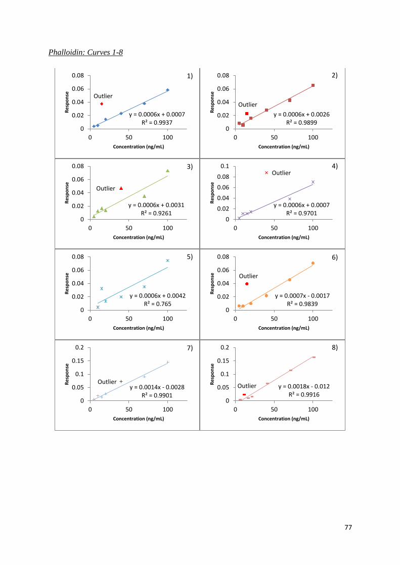
77

Phalloidin: Curves 1-8

Outlier

y = 0.0006x + 0.0007 R² = 0.9937

0

0.02

0.04

0.06

0.08

0 50 100

Re

spo

nse

Concentration (ng/mL)

1)

Outlier

y = 0.0006x + 0.0026 R² = 0.9899

0

0.02

0.04

0.06

0.08

0 50 100

Re

spo

nse

Concentration (ng/mL)

2)

Outlier

y = 0.0006x + 0.0031 R² = 0.9261

0

0.02

0.04

0.06

0.08

0 50 100

Re

spo

nse

Concentration (ng/mL)

3) Outlier

y = 0.0006x + 0.0007 R² = 0.9701

0

0.02

0.04

0.06

0.08

0.1

0 50 100

Re

spo

nse

Concentration (ng/mL)

4)

y = 0.0006x + 0.0042 R² = 0.765

0

0.02

0.04

0.06

0.08

0 50 100

Re

spo

nse

Concentration (ng/mL)

5)

Outlier

y = 0.0007x - 0.0017 R² = 0.9839

0

0.02

0.04

0.06

0.08

0 50 100

Re

spo

nse

Concentration (ng/mL)

6)

Outlier y = 0.0014x - 0.0028

R² = 0.9901 0

0.05

0.1

0.15

0.2

0 50 100

Re

spo

nse

Concentration (ng/mL)

7)

Outlier y = 0.0018x - 0.012 R² = 0.9916

0

0.05

0.1

0.15

0.2

0 50 100

Re

spo

nse

Concentration (ng/mL)

8)

78

Appendix 3: Data Generated from ANOVA Single Factor Analysis

α-amanitin:

Groups Count Sum Average Variance

Calibrator 1 8 0.283239 0.035404858 0.000304

Calibrator 2 8 0.240893 0.030111621 0.009713

Calibrator 3 6 0.169522 0.028253623 0.000557

Calibrator 4 8 0.015989 0.001998635 0.003479

Calibrator 5 6 -0.22365 -0.03727432 0.023767

Calibrator 6 6 -0.96215 -0.16035899 0.019318

Calibrator 7 8 1.191917 0.148989602 0.310188

Source of

Variation

SS df MS F P-value F crit

Between

Groups

0.352066535 6 0.058677756 1.015758 0.427934 2.318498

Within

Groups

2.484001114 43 0.057767468

Total 2.83606765 49

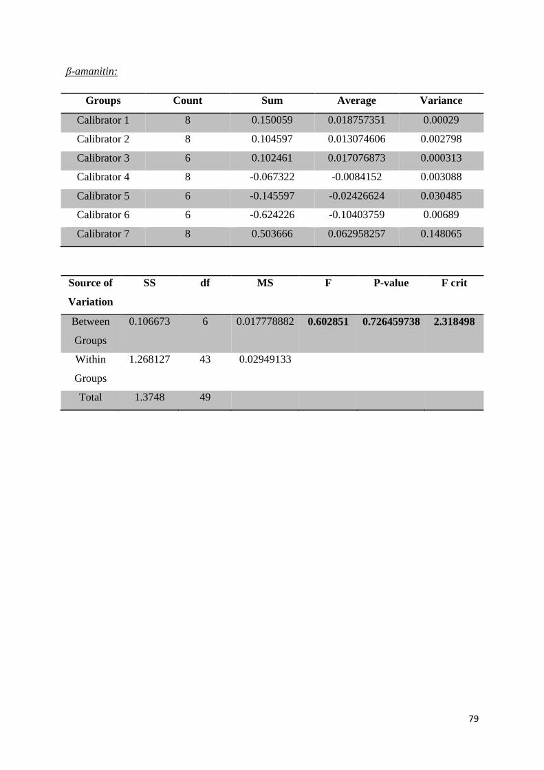
79

β-amanitin:

Groups Count Sum Average Variance

Calibrator 1 8 0.150059 0.018757351 0.00029

Calibrator 2 8 0.104597 0.013074606 0.002798

Calibrator 3 6 0.102461 0.017076873 0.000313

Calibrator 4 8 -0.067322 -0.0084152 0.003088

Calibrator 5 6 -0.145597 -0.02426624 0.030485

Calibrator 6 6 -0.624226 -0.10403759 0.00689

Calibrator 7 8 0.503666 0.062958257 0.148065

Source of

Variation

SS df MS F P-value F crit

Between

Groups

0.106673 6 0.017778882 0.602851 0.726459738 2.318498

Within

Groups

1.268127 43 0.02949133

Total 1.3748 49

80

Phalloidin:

Groups Count Sum Average Variance

Calibrator 1 7 -0.00145 -0.00021 4.13637E-06

Calibrator 2 7 -0.00535 -0.00076 2.85825E-05

Calibrator 3 5 0.009831 0.001966 8.2987E-05

Calibrator 4 8 -0.03646 -0.00456 2.11052E-05

Calibrator 5 5 -0.04202 -0.0084 0.000357116

Calibrator 6 8 -0.1198 -0.01498 0.000906842

Calibrator 7 8 -0.07814 -0.00977 0.001629367

Source of

Variation

SS df MS F P-value F crit

Between

Groups

0.001543 6 0.000257 0.53105564 0.781416656 2.329771

Within

Groups

0.019858 41 0.000484

Total 0.021401 47

81

Appendix 4: Signal to noise (S/N) Data

Curve α-amanitin (Cal 1) β-amanitin (Cal 1) Phalloidin (Cal 3)

Curve 1 5.06 3.16 2.43

Curve 2 5.15 5.40 1.68

Curve 3 6.62 4.60 4.07

Curve 4 12.53 5.95 3.19

Curve 5 5.60 4.99 2.17

Curve 6 7.64 4.47 2.06

Curve 7 8.47 5.97 2.28

Curve 8 7.25 3.96 2.02

Average 7.29 4.81 2.49