Towards texture classification in real scenes

Paul Southam and Richard HarveySchool of Computing Sciences

University of East AngliaNorwich, UK

{pauls, rwh}@cmp.uea.ac.uk

Abstract

Two new texture features, based on morphological scale-space processors areintroduced. The new methods are shown to have good performance over avariety of tests. We demonstrate that if texture classifies are to be used in realworld scenes, then the choice of test is critical and that Brodatz-like tests areunlikely to represent reality.

1 Introduction

There are a number of motivations for studying texture classification. Sometimes thereis a real problem such as the classification of marble, sorting of wood, classification ofcarpet and so on. Other times one is interested to study a stylised classification problemas a convenient benchmark. This latter position is more difficult since there is a naggingdoubt that results on stylised experiments will not extrapolate to reality. This paper ex-amines this doubt, using available texture databases. The well known texture databasesare Brodatz; VisTex; MeasTex and Outex (see [6] for a summery). CURet [3], althoughdesigned for a different task, might also be mentioned.

Bro

datz

Vis

Tex

Mea

sTex

Out

ex

CU

ReT

No. Classes 100–112∗ 19 4 29 61

No. Images per class 1–4∗ 1–20 4–25 1–47 205†

Evaluation Framework? × ×√ √

×Defined test/training data? × ×

√ √×

Unique copy? ×√ √ √ √

Table 1: Available texture databases (∗ Depending on implementation,† At differing angleand illuminant.)

With the exception of Brodatz, Table 1 shows that all are available for downloadwhich ensures that each experiment is performed with identical texture samples. Bro-datz, although the most common, is available as a book and since different methods and

Figure 1: Three Outex natural scene images (left column), hand-segmented ground-truthsupplied with the database (middle column) and our new ground-truth (right column).Note that each region has lighting, scale and rotation variations.

equipment were used for digitisation there are several electronic versions at different file,size, format and resolution; all of which affect results1. Brodatz, VisTex and CuRET donot have pre-defined test and training data which hinders comparisons of different clas-sification methods. See [10], for example, where different test and training data lead toconflicting results. MeasTex and VisTex have a few samples and classes. VisTex is nolonger maintained. In [11] it is claimed that the MesTex classes are non-overlapping fora greater number of methods. Therefore Outex is the best dataset for comparing textureclassifiers and should be the database of choice for comparing texture classifiers.

Currently Outex has 319, grey-scale and colour textures spanning 29 classes. Theimages are organised intotest suitessetup for, classification, segmentation, and retrieval.The test suites are designed to examine illumination, scale, rotation and colour invariance.There is also a natural scenes test suite which contains 20 colour images (2272× 1704pixels) of scenes under varying illumination and orientation. There are five texture classes,sky, trees, grass, road and buildings which are defined through hand-labelled ground-truth. Examples of the scene and ground truth images are in Figure 1.

To compare texture classifiers that are restricted to rectangular windows, we providealternative hand-segmented ground truth also shown in Figure 1. We use the same classlabels as the original ground-truth.

1[9] for example shows images that have an accidental gray-scale inversion compared to the book.

1

Input Signal Difference Granularity

2

m

+

-

+

-

+

-

G1

G2

Gm

Figure 2: The structure of a sieve decomposition whereϕ is a filtering operator chosenfrom a set [1, 2]. Non-zero regions in the output are calledgranulesand the set of granulesis called thegranularity domainin an analogy to granulometries.

2 Methods

There are a very large number of proposed methods of classifying texture. Here we at-tempt to represent performance via three techniques that have been reported to work wellin the literature.

The first benchmark is the dual-tree complex wavelet transform (DTCWT) [5], whichis known to have better shift invariance and directional selectivity than conventionalwavelets. The DTCWT decomposes an image into eight sub-bands: two low-pass andsix high-pass at orientations of±15◦,±45◦,±75◦. Decomposing to three levels produces8+ 82 + 83 bands. The sample mean and standard deviation of absolute values of thesebands are taken to form a feature vector of 336 elements.

The second benchmark is the local binary pattern (LBP) [7] method, which producesfeatures based upon the spatial structure of an image using absolute grey-level intensitydifferences between neighbouring pixels. It works by passing a 3×3 window over everypixel in the texture. Pixels that have intensities higher than or equal to, the target pixel aremasked off. These masked pixels are assigned weightings that are summed to producea LBP-score within the range 0−→ 255. Hence LBP produces a feature vector of 256elements.

The third benchmark uses co-occurrence matrices (co-occ) introduced in [4]. Co-occurrence matrices extract second order statistics based upon the vector between twopixels in an image. Once the matrix of frequencies has been created, a number of featurescan be derived from it. We use 12 features representing energy, contrast, entropy andhomogeneity at orientations of 0◦,90◦ and 45◦.

We also introduce new methods based upon the morphological operator known asthe sieve. Sieves were originally defined as one-dimensional systems [1] but were laterextended ton-dimensional filters [2] that adopt techniques from graph morphology. Theyare cascades of morphological scale-space operators that remove intensity extrema at a

specific scale via the structure shown in Figure 2.In the first new method, denoted (2D-sieve),ϕ is a 2DM -filter [2] which filters the

image using a morphological opening followed by a morphological closing in one opera-tion. This method produces a decomposition that, ignoring sampling errors, is invariant torotation. At small scales, the processor tends to remove noise; then, as the scale increases,texture; then, objects within the scene as in, for example, Figure 3.

A B C

D E F

Figure 3: An original image (A) sieved using a 2D-sieve to scales 15(B), 90(C), 251(D),2000(E) and 5000(F). Each image has fewer intensity extrema than its predecessor. A fulldecomposition may be summed to re-create the original thus the sieve is a transform ofthe original image.

The second new method (1D-sieve) is similar, but now there is an additional parame-ter: the orientation at which the filter is applied. Hereϕ is a 1D recursive median filter, asin [13] for example, at orientations of 0◦,±30◦,±45◦,+90◦. The 2D-sieve decomposesan image by scale equal to the area of intensity extrema, where as the 1D-sieve decom-poses by length. Figure 4 shows an example 1D-sieve decomposition from which we cansee that the decomposition is anisotropic.

The features from both new methods are based ongranules. In [2], granule imagesare defined as the difference between successive sieve outputs,Gn = ϕn−ϕn−1 whereϕn

is thenth stage in the serial structure shown in Figure 2. There are thus a great numberof granule images. TheGn are a transform of the texture which can be reconstructedthrough a simple summation. Here, each texture image is sieved to a few scales,[s1 . . .sN]where log10sn are equispaced between 0 and log10P, whereP = 30 is chosen to removeall textural information from all images. The difference between these images are termedchannels, Cn = ϕsn − ϕsn−1. We chooseN = 5 to give 5 channels. The magnitude ofthe channel images as a function of scale is an indicator of the scale-distribution of thetexture features. The sample mean, standard deviation and skewness of the magnitude ofthe granule images may be used as features. Thus the 2D-sieve has 15 features and the1D-sieve has 90 features.

A B C

D E F

Figure 4: An original image (A) sieved using a 1D-sieve to scales 1(B), 5(C), 16(D),29(E) and 50(F) at an angle of 45◦.

Figure 5 (left) hows the sample mean for three texture classes using a 2D-sieve.Thestandard deviation and skewness are not show here but have similar variations. Finer scaletextures have peak responses at lower scales and the coarser textures have peaks at higherscales.

1 2 3 4 5

−5

0

5

10

Feature Index

Fea

ture

Am

plit

ud

e

Class AClass BClass C

1 2 3 4 50

0.51

1.52

2.53

3.54

4.5

Feature Index

Fea

ture

Am

plit

ud

e

30 deg60 deg90 deg

Figure 5: Left: Sample mean against feature index of three texture classes A,B and Cshown in Figure 7. Right: The sample mean of a texture class D shown in Figure 7 at 30◦,60◦ and 90◦. Feature index is correlated with scale: 1 is scale (0-1), 2 is scale (1-2), 3 isscale (2-5), 4 is scale (5-13) and 5 is scale (13-30).

Figure 5 (right) also shows how the sample mean varies for a stripy texture such asclass A (shown in Figure 7) using a 1D-sieve applied at several angles. At 90◦ where the

scan-line runs along the direction of the texture, the intensity variation is less resulting ina flatter response.

Fast algorithms exist for sieves, and in practice a full decomposition of a domesticvideo image takes a couple of hundred ms. In all methods we compute the covariancematrix over the training data and apply principal component analysis (PCA) retaining allcomponents: since we have found that this always improves performance on all methodsand all databases.

3 Results

The first test,Test-1, uses the OutexTC 00000 test suite. It contains 100 leave-out-halfcross validation, classification experiments (different permutations of 240 testing and 240training data) of 480 images. There are 20 samples of 24 texture classes. Classification isvia a k-nearest neighbour classifier (elsewhere [12] it has been shown that k = 1, Euclideandistance is the best choice for this test). Table 2 shows the results. The success rate ofthe LBP method differs from [7] (0.995) because in our experiments we are not usinga histogram distance measure. The results for Gabor wavelets and Gaussian MarkovRandom Fields are taken directly from [8] and it is not clear what classifier or distancemeasure is being used.

1D-Sieve 2D-Sieve DTCWT LBP Co-occ Gabor GMRF

x̄ 0.998 0.962 0.999 0.986 0.946 0.995 0.961

max 1 0.992 1 0.996 0.983 1 0.992

min 0.988 0.933 0.988 0.967 0.900 0.983 0.925

σ 0.0034 0.0103 0.0019 0.0070 0.0154 0.5 1.3

σ ′ 0.00034 0.00103 0.00019 0.00070 0.00154 0.05 0.13

f 90 15 336 256 12 ?? ??

Table 2: Mean success rate, ¯x, over 100 trials, max and min success rate, standard devia-tion σ , standard error of the meanσ ′ = σ \

√N and number of featuresf for Outex test

suite OutexTC 00000. The results for the Gabor and GMRF methods are taken from [8]which doesn’t specify the number of features used.

Table 3 shows the result of using McNemars’s test on each trial at a significance ofα = 0.05. The 1D-sieve and DTCWT are indistinguishable at a significance for all 100tests with OutexTC 00000.

Using PCA to reduce feature dimensionality improves the 1D-sieve success rate to0.999 which is similar to the DTCWT but with only 40 features. The affect of applyingPCA to the DTCWT does not improve performance but maintains a 0.999 success rateusing 77 features. Figure 6 shows the affect on success rate of reducing the number offeatures using PCA. The 1D-sieve has the highest success rate for the fewest features.

To test for noise-invariance we repeat the experiments using the OutexTC 00000 testsuite. Multiplicative noise (n) is added to each test image (I ) resulting in a noisy imageJ = I + n∗ I , wheren is uniformly distributed random noise with mean 0 and variance

1D-Sieve 2D-Sieve DTCWT LBP Co-occ

1D-sieve x 90 0 10 96

2D-sieve - x 93 22 10

DTCWT - - x 12 98

LBP - - - x 67

Table 3: The number of times out of the OutexTC 00000 100 trials that we can confi-dently (α = 0.05) reject the null hypothesis that the two data distributions are drawn fromthe same source.

[V1 · · ·Vk] wherelog10Vk are equispaced between 0 and 0.0115. Figure 6 show that the1D- and 2D-sieve are the most invariant to multiplicative noise2.

100

101

1020.2

0.4

0.6

0.8

1

Number of Features

Su

cces

s R

ate

2D sieveCo−occLBP1D sieveDTCWT

0 0.002 0.004 0.006 0.008 0.01 0.0120

0.2

0.4

0.6

0.8

1

Multiplicative Noise Variance

Su

cces

s R

ate

Co−occDTCWTLBP1D−sieve2D−sieve

Figure 6: Success rate against log number of features (left) and Success rate against mul-tiplicative noise variance (right)

In the real world the orientation of a texture class may be unknown. So inTest-2weuse OutexTC 00010 to test for rotation invariance. This test suite contains textures underconstant illuminant and scale but with rotations of 00◦,05◦,10◦,15◦,30◦,45◦,60◦,75◦,90◦.There are 480 training images of 24 classes and 3840 test images. Table 4 shows the re-sults. It appears that the performance of some methods degrades badly under unknownrotation. The 2D-sieve is now the best performing.

1D-Sieve 2D-Sieve DTCWT LBP Co-occ

x̄ 71.80 94.30 55.63 50.91 69.17

f 90 30 336 256 12

Table 4: Mean success rate, ¯x, and number of featuresf for rotation-variant Outex testsuite OutexTC 00010.

2We have similar results, not reported here, for additive Gaussian noise.

Test-3 concerns natural scenes. Rectangular regions (right column of Figure 1) arecropped from images of natural scenes to give texture images of the type shown in thecentre row of Figure 3. There are 80 images which is too few for hold-out so they areused in 80 leave-out-one cross-validation experiments. The top half of Table 5 shows theresults with a knn classifier (k = 3, Euclidean distance).

Test-4uses the Outex natural scenes database but now the ground-truth is polygonal.There are a total of 91 labelled regions so again we use leave-out-one cross-validation.Table 5 shows the success rate across all classes, with a knn classifier (k = 3, Euclideandistance). Also shown is the number of samples per class. Not all texture methods areeasily applicable to this set because the regions are non-rectangular. We therefore restrictthe comparison to the LBP and sieve methods because, for these, we can generate thefiltered images, apply the hand-segmented region as a mask, and generate a feature foreach region. In Test-3 and Test-4 the best performing method on a per-class-winner oroverall mean basis is the 2D-sieve.

sky

tree

bush

gras

s

road

build

ing

mea

n

Test-3No. Samples 14 15 10 19 14 8

1D-sieve 1 0.933 0.4 0.84 0.71 0.38 0.712D-sieve 1 1 0.5 0.63 0.71 0.5 0.72DTCWT 1 0.8 0.3 0.84 0.64 0.63 0.70

LBP 0.79 0.6 0.5 0.53 0.57 0.13 0.52co-occ 0.93 0.93 0.3 0.37 0.57 0.5 0.60

Test-4No. Samples 14 17 15 20 16 9

1D-sieve 0.79 0.59 0.2 0.6 0.38 0 0.422D-sieve 1 0.82 0.53 0.65 0.88 0.33 0.7

LBP 0.64 0.76 0.6 0.4 0.81 0.22 0.57

Table 5: Table shows number of samples per class, mean success rate per class and overallmean success rate for the Outex natural scene database.

4 Conclusions

This paper presents new texture classifiers and compares their performance to some wellknown benchmarks. The first test, Test-1, was quite conventional and is representative ofa large number of texture evaluations in the literature. Had we stopped at this point then,the conclusion would be that one of the new methods, 1D-sieve, was as good as one ofthe benchmarks (DTCWT) but used fewer features.

Test-2 represents the situation where the orientation is unknown. Now, the previouslybest performing methods degrade. The DTCWT is now the second worst method andthe 1D-sieve is out-performed by the 2D-sieve which we were confident was not the bestmethod previously.

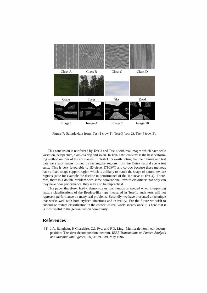
Class A Class B Class C Class D

Grass Trees Sky Road

Image 1 Image 4 Image 7 Image 10

Figure 7: Sample data from: Test-1 (row 1), Test-3 (row 2), Test-4 (row 3).

This conclusion is reinforced by Test-3 and Test-4 with real images which have scalevariation, perspective, class-overlap and so on. In Test-3 the 2D-sieve is the best perform-ing method on four of the six classes. In Test-3 it’s worth noting that the training and testdata were sub-images formed by rectangular regions from the Outex natural scene testsuite. This is very favourable to 1D-sieve, DTCWT and co-ooc because these methodshave a fixed-shape support region which is unlikely to match the shape of natural textureregions (note for example the decline in performance of the 1D-sieve in Test-4). There-fore, there is a double problem with some conventional texture classifiers: not only canthey have poor performance, they may also be impractical.

This paper therefore, firstly, demonstrates that caution is needed when interpretingtexture classifications of the Brodatz-like type measured in Test-1: such tests will notrepresent performance on many real problems. Secondly, we have presented a techniquethat works well with both stylised situations and in reality. For the future we wish toencourage texture classification in the context of real world scenes since it is here that itis most useful to the general vision community.

References

[1] J.A. Bangham, P. Chardaire, C.J. Pye, and P.D. Ling. Multiscale nonlinear decom-position: The sieve decomposition theorem.IEEE Transactions on Pattern Analysisand Machine Intelligence, 18(5):529–539, May 1996.

[2] J.A. Bangham, R. Harvey, P.D. Ling, and R.V. Aldridge. Morphological scale-spacepreserving transforms in many dimensions.Journal of Electronic Imaging, 5:283–299, 1996.

[3] CUReT. http://www1.cs.columbia.edu/cave/curet/.

[4] R. Haralick. Statistical and structural approaches to texture. InProccedings of IEEE,volume 67, pages 786–804, 1979.

[5] N. Kingsbury. Image processing with complex wavelets. InPhil. Trans. RoyalSociety London A, September 1999, on a Discussion Meeting on Wavelets: the keyto intermittent information?, London, February 24-25, 1999.

[6] T. Ojala, T. Maenpaa, M. Pietikainen, J. Viertola, J. Kyllonen, and S. Huovinen. Ou-tex - new framework for empirical evaluation of texture analysis algorithms. InProc.16th International Conference on Pattern Recognition, Quebec, Canada, volume 1,pages 701–706, 2002.

[7] T. Ojala, M. Pietikanien, and D. Harwood. A comparative study of texture measureswith classification based on feature distributions.Pattern Recognition, 29:51–59,1996.

[8] Outex. http://www.outex.oulu.fi.

[9] C.-M. Pun and M.-C. Lee. Log-polar wavelet energy signatures for rotation andscale invariant texture classification.IEEE Transactions on Pattern Analysis andMachine Intelligence, 25(5):590–603, 2003.

[10] T. Randen and J. Husoy. Filtering for texture classification: A comparative study.IEEE Transactions on Pattern Analysis and Machine Intelligence, 21(4):291–310,1999.

[11] S. Singh and M. Sharma. Texture analysis experiments with meastex and vistexbenchmarks.Lecture Notes in Computer Science, 2013:417–424, 2001.

[12] Paul Southam and Richard Harvey. Compact rotation-invariant texture classification.In International Conference on Image Processing (ICIP 2004), pages 3033–3036.IEEE, 24–27 Oct 2004.

[13] R. Zwiggelaar, T.C. Parr, J.E. Schumm, I.W. Hutt, S.M. Astley, C.J. Taylor, andC.R.M. Boggis. Model-based detection of spiculated lesions in mammograms.Med-ical Image Analysis, 3(1):39–62, 1999.