Towards Self-Organizing Wireless Networks: Adaptive ... · Zusammenfassung Das Konzept...
153
Towards Self-Organizing Wireless Networks: Adaptive Learning, Resource Allocation, and Network Control vorgelegt von Diplom-Ingenieur Martin Kasparick geb. in Berlin von der Fakult¨ at IV - Elektrotechnik und Informatik der Technischen Universit¨ at Berlin zur Erlangung des akademischen Grades Doktor der Ingenieurwissenschaften - Dr.Ing. - genehmigte Dissertation Promotionsausschuss: Vorsitzende: Prof. Anja Feldmann, Ph.D. Gutachter: Prof. Dr. Slawomir Sta´ nczak Gutachter: Prof. Dr. Rudolf Mathar (RWTH Aachen) Gutachter: PD Dr. habil. Gerhard Wunder Tag der wissenschaftlichen Aussprache: 21. Dezember 2015 Berlin 2016
Transcript of Towards Self-Organizing Wireless Networks: Adaptive ... · Zusammenfassung Das Konzept...

Towards Self-Organizing WirelessNetworks: Adaptive Learning, Resource
Allocation, and Network Control
vorgelegt von
Diplom-Ingenieur
Martin Kasparick
geb. in Berlin
von der Fakultat IV - Elektrotechnik und Informatik
der Technischen Universitat Berlin
zur Erlangung des akademischen Grades
Doktor der Ingenieurwissenschaften
- Dr.Ing. -
genehmigte Dissertation
Promotionsausschuss:
Vorsitzende: Prof. Anja Feldmann, Ph.D.
Gutachter: Prof. Dr. S�lawomir Stanczak
Gutachter: Prof. Dr. Rudolf Mathar (RWTH Aachen)
Gutachter: PD Dr. habil. Gerhard Wunder
Tag der wissenschaftlichen Aussprache: 21. Dezember 2015
Berlin 2016


Abstract
The concept of self-organizing networks is a promising approach to address funda-
mental challenges in current and future wireless networks. Not least the dense and
heterogeneous nature of the networks, the scarcity of resources, and high costs of man-
ual configurations necessitate efficient self-organization techniques that autonomously
adapt crucial system parameters to changing traffic and network conditions. This thesis
is concerned with key aspects of self-organizing networks, in particular the generation
of the required knowledge, and the design of particular self-optimization mechanisms
in wireless networks.
Any self-organization functionality depends on knowledge about the current system
state. The first part of this thesis deals with learning techniques that enable a wide
range of self-optimization and self-configuration functions. In particular, we investi-
gate the generation of knowledge in form of geographical radio maps. The radio maps
are generated based on user measurements, which arrive sequentially and continuously
over time. To process this persistent data stream, low-complexity online estimation
and learning techniques are needed. We employ powerful kernel-based adaptive filter-
ing techniques, which are robust to measurement errors. To demonstrate how addi-
tional context information can be taken into account, we show, how knowledge about
anticipated user routes can be incorporated in the learning process. Moreover, we in-
vestigate the performance of the algorithms in different scenarios; more specifically, we
apply these techniques to the problem of path-loss estimation and to the problem of
estimating interference maps. Such radio maps are considered invaluable for network
planning and optimization tasks. Furthermore, we demonstrate how interference maps
can be used to support network-assisted device-to-device communications.
In addition to the aspect of knowledge generation, the second and third part of the
thesis deal with particular self-optimization techniques. The second part of the thesis
is concerned with self-optimization in interference-limited networks, motivated by the
trend towards densely deployed heterogeneous cellular networks, which are expected to
become prevalent in the next generations of wireless communication systems. Especially
in multi-antenna networks, inter-cell interference coordination poses a major challenge,
since not only temporal and spectral resources, but also the spatial dimension has to
be taken into account. To address this challenge, we propose distributed coordination
i

ii Abstract
algorithms for inter-cell (and intra-cell) interference coordination in SDMA-based cel-
lular networks. Based on a local maximization of a network-wide utility function over
average user rates, the proposed algorithms autonomously adapt the transmit power
budgets of particular resources. Using system-level simulations, we show that, espe-
cially in networks with high user mobility, the control of average power budgets for
particular time-frequency-space resources is superior to a direct control of the transmit
powers.
In the last part of the thesis, we consider more general network topologies with
a stochastic traffic modeling. We derive a framework to design network-layer control
policies based on a suitable cost function. Thereby, the framework adapts scheduling
and routing decisions to the requirements of different services and applications, while
ensuring queueing theoretic stability. As particular applications, we investigate the
cost function based control approach for networks with minimum buffer constraints
(e.g., in case of multimedia streaming), and for networks with energy limited nodes. In
addition, we show how existing cross-layer control algorithms can be adapted to our
control framework.

Zusammenfassung
Das Konzept selbstorganisierender Kommunikationsnetze, die zentrale Systemparam-
eter automatisch an veranderliche Datenverkehrs- und Netzbedingungen anpassen, ist
ein vielversprechender Ansatz um fundamentalen Herausforderungen in aktuellen und
zukunftigen drahtlosen Kommunikationsnetzen zu begegnen. Insbesondere die dichte
und heterogene Natur zukunftiger drahtloser Netze, die Begrenztheit der Kommunika-
tionsressourcen, sowie hohe Kosten manueller Konfiguration und Wartung werden den
Einsatz von Selbstorganisationstechniken unverzichtbar machen. Diese Arbeit befasst
sich mit zentralen Aspekten selbstorganisierender Kommunikationsnetze und unter-
sucht dabei sowohl die Schaffung einer Informationsgrundlage als auch den Entwurf
konkreter Selbstoptimierungsmechanismen.
Jeder Algorithmus zur Selbstorganisation ist auf aktuelle Informationen uber den
Zustand des Gesamtsystems angewiesen. Im ersten Teil der Arbeit werden maschinelle
Lernverfahren entwickelt um diese Informationen autonom erzeugen zu konnen und
damit die Voraussetzung fur zahlreiche Selbstoptimierungs- und Selbstorganisationsver-
fahren zu schaffen. Speziell werden Algorithmen zur Erzeugung einer Wissens- und
Entscheidungsgrundlage in Form von ortsbasierten Radiokarten formuliert und analysiert.
Die Erzeugung der Radiokarten basiert auf der Verarbeitung nutzergenerierter Mess-
daten, welche kontinuierlich und sequentiell zur Verfugung gestellt werden. Um diesen
kontinuierlichen Datenstrom verarbeiten zu konnen, werden echtzeitbasierte Schatz-
und Lernverfahren mit niedriger Komplexitat benotigt. Zu diesem Zweck wird der
Einsatz kernelbasierter adaptiver Filtertechniken vorgeschlagen und evaluiert, welche
zudem eine hohe Robustheit gegenuber Messungenauigkeiten besitzen. Beispielhaft fur
die Einbeziehung zusatzlich verfugbarer Kontextinformationen wird gezeigt, wie die
Kenntnis voraussichtlicher Nutzerrouten in den Lernprozess integriert werden kann.
Die Performanz der entwickelten Algorithmen, insbesondere im Zusammenhang mit
der Schatzung von Pfadverlustkarten und Interferenzkarten, wird im Hinblick auf ver-
schiedene Netz- und Anwendungsszenarien untersucht. Derartige Radiokarten sind
speziell fur die adaptive Netzplanung und -optimierung von großer Bedeutung. Daruber
hinaus wird gezeigt, wie insbesondere Interferenzkarten zur Unterstutzung von net-
zgestutzter Gerat-zu-Gerat-Kommunikation eingesetzt werden konnen.
Erganzend zum Aspekt der Wissensgenerierung werden im zweiten und dritten
iii

iv Zusammenfassung
Teil der Arbeit konkrete Selbstorganisationsverfahren untersucht. Motiviert durch
den anhaltenden Trend zu immer dichteren heterogenen zellularen Netzen, behan-
delt der zweite Teil dieser Arbeit Selbstoptimierungsverfahren zur Koordinierung von
Inter-Zell-Interferenz in interferenzbegrenzten Netzen. Die Koordinierung von Inter-
Zell-Interferenz bedeutet insbesondere in Mehrantennensystemen eine große Heraus-
forderung, da nicht nur Zeit- und Frequenzressourcen sondern auch die raumliche
Dimension in die Koordinierung mit einbezogen werden muss. Fur derartige zellu-
lare Mehrantennennetze werden selbstorganisierende verteilte Koordinationsalgorith-
men entworfen, welche die Sendeleistungsbudgets einzelner Ressourcen basierend auf
der Maximierung einer netzweiten, uber mittleren Nutzerubertragungsraten definierten,
Nutzwertfunktion anpassen. Dabei wird gezeigt, dass es in Netzen mit mobilen Nutzern
vorteilhafter ist, mittlere Sendeleistungsbudgets zu adaptieren, als die Sendeleistungen
direkt zu kontrollieren.
Im letzten Teil dieser Arbeit werden allgemeinere Netztopologien mit stochastis-
cher Modellierung der Datenaufkommen betrachtet. Vorgestellt wird ein Konzept zum
Entwurf von Kontrollstrategien auf der Netzwerkschicht, die, auf Basis einer geeignet
gewahlten Kostenfunktion, Scheduling- und Routingentscheidungen an die Anforderun-
gen vorherrschender Anwendungen und Dienste anpassen konnen und gleichzeitig Sta-
bilitat im Sinne der Warteschlangentheorie garantieren. Als konkrete Anwendungen
werden der kostenfunktionsbasierte Entwurf von Kontrollstrategien fur Netze mit Min-
destanforderungen an Pufferfullstande (z.B. im Fall von Multimedia-Streaming), sowie
fur Netze aus Knoten mit begrenzter Energie untersucht. Daruber hinaus wird gezeigt,
wie bestehende Algorithmen zur schichtubergreifenden Kontrolle an das vorgestellte
Konzept angepasst werden konnen.

Acknowledgements
First of all, I would like to thank my advisors PD Dr.-Ing. habil. Gerhard Wunder and
Prof. Slawomir Stanczak, who made my research possible during my time at TU-Berlin
and Fraunhofer HHI, and who constantly guided and supported me during the course
of my PhD studies. Also, I am very grateful to Prof. Rudolf Mathar for investing the
time to review this thesis.
Moreover, I want to thank all my colleagues at the Fraunhofer Heinrich-Hertz-
Institut and the Technical University of Berlin for many discussions and the great
working environment. Especially, I would like to thank Dr. Renato Cavalcante for
many interesting scientific discussions and his guidance during the last years.
I would like to express my sincere gratitude to my family and friends for their steady
encouragement, but my special gratitude goes to my wife, Claudia; without her endless
patience and support, this thesis would never have been possible.
v


Table of Contents
1 Introduction 1
1.1 Motivation . . . . . . . . . . . . . . . . . . . . . . . . . . . . . . . . . . 1
1.2 Outline and Contributions of the Thesis . . . . . . . . . . . . . . . . . . 4
1.3 Notations . . . . . . . . . . . . . . . . . . . . . . . . . . . . . . . . . . . 7
2 Adaptive Learning for Self-Organizing Communication Networks 9
2.1 Preliminaries and Essential Convex Analysis Tools . . . . . . . . . . . . 11
2.2 Online Reconstruction of Radio Maps With Side Information . . . . . . 14
2.2.1 The APSM-Based Algorithm . . . . . . . . . . . . . . . . . . . . 16
2.2.2 The Multi-Kernel Approach . . . . . . . . . . . . . . . . . . . . . 19
2.2.3 Computational Complexity . . . . . . . . . . . . . . . . . . . . . 22
2.2.4 Adaptive Weighting . . . . . . . . . . . . . . . . . . . . . . . . . 22
2.3 Applications . . . . . . . . . . . . . . . . . . . . . . . . . . . . . . . . . . 26
2.3.1 Application to Path-loss Learning . . . . . . . . . . . . . . . . . 27
2.3.2 Interference Estimation With Application to Device-to-Device
Communications . . . . . . . . . . . . . . . . . . . . . . . . . . . 43
2.3.3 Discussion . . . . . . . . . . . . . . . . . . . . . . . . . . . . . . . 52
3 Resource Allocation in Interference-Limited Networks 55
3.1 System Model . . . . . . . . . . . . . . . . . . . . . . . . . . . . . . . . . 57
3.2 Network Utility Maximization . . . . . . . . . . . . . . . . . . . . . . . . 59
3.3 Interference Mitigation by Autonomous Distributed Power Control . . . 61
3.3.1 Opportunistic Algorithm . . . . . . . . . . . . . . . . . . . . . . 63
3.3.2 Virtual Subband Algorithm . . . . . . . . . . . . . . . . . . . . . 65
3.3.3 Cost-Based Algorithm . . . . . . . . . . . . . . . . . . . . . . . . 67
3.4 Performance Evaluation . . . . . . . . . . . . . . . . . . . . . . . . . . . 70
3.4.1 Simulation Configuration . . . . . . . . . . . . . . . . . . . . . . 70
3.4.2 Baseline Algorithm . . . . . . . . . . . . . . . . . . . . . . . . . . 71
3.4.3 Global Utility Versus Cell-Edge User Performance . . . . . . . . 72
3.5 Global Optimality: A Branch-and-Bound Based Solution . . . . . . . . . 74
3.5.1 Bounding . . . . . . . . . . . . . . . . . . . . . . . . . . . . . . . 76
3.5.2 Numerical Results . . . . . . . . . . . . . . . . . . . . . . . . . . 78
vii

viii TABLE OF CONTENTS
3.6 Discussion . . . . . . . . . . . . . . . . . . . . . . . . . . . . . . . . . . . 79
4 Flexible Stochastic Network Control 81
4.1 Preliminaries . . . . . . . . . . . . . . . . . . . . . . . . . . . . . . . . . 83
4.1.1 Queueing Model . . . . . . . . . . . . . . . . . . . . . . . . . . . 84
4.1.2 Stability . . . . . . . . . . . . . . . . . . . . . . . . . . . . . . . . 86
4.1.3 Throughput-Optimal Control: The MaxWeight Policy . . . . . . 86
4.1.4 Cost Minimization and Myopic Control . . . . . . . . . . . . . . 87
4.1.5 Generalized MaxWeight . . . . . . . . . . . . . . . . . . . . . . . 88
4.2 Control Policy and Cost Function Design . . . . . . . . . . . . . . . . . 89
4.2.1 Cost Function Choice . . . . . . . . . . . . . . . . . . . . . . . . 91
4.2.2 Policy Design . . . . . . . . . . . . . . . . . . . . . . . . . . . . . 92
4.2.3 Example: Controlling a Network of Queues in Tandem . . . . . . 94
4.2.4 A Pick and Compare Approach for Reducing Complexity . . . . 94
4.3 Applications . . . . . . . . . . . . . . . . . . . . . . . . . . . . . . . . . . 96
4.3.1 Application to Large Multimedia Networks . . . . . . . . . . . . 96
4.3.2 Energy-Efficient Network Control . . . . . . . . . . . . . . . . . . 101
4.3.3 Application to Cross-Layer Control . . . . . . . . . . . . . . . . . 103
4.3.4 Discussion . . . . . . . . . . . . . . . . . . . . . . . . . . . . . . . 111
5 Summary and Outlook 113
5.1 Summary . . . . . . . . . . . . . . . . . . . . . . . . . . . . . . . . . . . 113
5.2 Outlook and Future Research . . . . . . . . . . . . . . . . . . . . . . . . 116
A Kriging Algorithm Summary 119
Acronyms 122

List of Figures
2.1 Exemplary radio maps with respect to two base stations . . . . . . . . . 10
2.2 Exemplary radio map from a network perspective . . . . . . . . . . . . . 11
2.3 Comparison of kernel-based algorithms’ performance in rural scenario . 29
2.4 Comparison of kernel-based algorithms’ performance in campus scenario 30
2.5 Original and estimated path-loss map in urban scenario . . . . . . . . . 33
2.6 Comparison of true path-loss and predicted path-loss in urban scenario . 34
2.7 Comparison of the MSE performance in urban scenario . . . . . . . . . 34
2.8 Impact of errors on the MSE performance in urban scenario . . . . . . . 35
2.9 Comparison of dictionary sizes using APSM and multikernel approach . 36
2.10 Effect of the algorithm parameters on the MSE in urban scenario . . . . 37
2.11 Madrid grid area and corresponding original and estimated path-loss data 39
2.12 Performance of kernel-based algorithms (error-free case) in heteroge-
neous network scenario . . . . . . . . . . . . . . . . . . . . . . . . . . . . 40
2.13 Performance of kernel-based algorithms (erroneous measurements) in
heterogeneous network scenario . . . . . . . . . . . . . . . . . . . . . . . 40
2.14 Estimated path-loss and coverage maps of an exemplary base station in
heterogeneous network scenario . . . . . . . . . . . . . . . . . . . . . . . 42
2.15 Snapshot of interference in simulator. . . . . . . . . . . . . . . . . . . . . 43
2.16 Screenshot of simulation environment for interference estimation . . . . 46
2.17 MSE between true interference matrix and approximation . . . . . . . . 47
2.18 Schematic illustration of see-through use-case. . . . . . . . . . . . . . . . 49
2.19 LOS performance of channel-aware algorithm in see-through use case . . 51
2.20 Comparison of frame error CDFs between LOS and NLOS scenario . . . 52
3.1 Conceptual illustration of spatial multiplexing . . . . . . . . . . . . . . . 58
3.2 Resource grid from the scheduler’s perspective . . . . . . . . . . . . . . 59
3.3 General network control approach . . . . . . . . . . . . . . . . . . . . . 61
3.4 Comparison of instantaneous powers with target power budgets . . . . . 70
3.5 Cell-edge user throughput vs. GAT in a fading environment . . . . . . . 73
3.6 Cell-edge user throughput vs. GAT in a static environment . . . . . . . 74
ix

x LIST OF FIGURES
3.7 Distributed power control vs. BNB-based solution for different interfer-
ence regimes . . . . . . . . . . . . . . . . . . . . . . . . . . . . . . . . . . 79
4.1 Exemplary queueing network . . . . . . . . . . . . . . . . . . . . . . . . 85
4.2 Cost function trajectories for a single buffer . . . . . . . . . . . . . . . . 92
4.3 Tandem network . . . . . . . . . . . . . . . . . . . . . . . . . . . . . . . 94
4.4 Queue trajectories with different cost functions in tandem queue network 95
4.5 Illustration of in-flight multimedia network . . . . . . . . . . . . . . . . 96
4.6 Schematic representation of the considered multimedia network . . . . . 97
4.7 Relative frequencies of buffer underflows with different cost functions . . 99
4.8 Relative frequencies of queue outages with different cost functions . . . 100
4.9 Relative frequencies of queue outages over the system bandwidth . . . . 101
4.10 Network of battery powered nodes . . . . . . . . . . . . . . . . . . . . . 102
4.11 Sum idle time over network load for different control policies . . . . . . 103
4.12 Illustration of Shannon rate and several convex approximations . . . . . 107
4.13 Average link powers over time using SCA-based power control . . . . . . 109
4.14 Average buffer states over time with and without power control . . . . . 109
4.15 Average cost over mean arrival rate and over time . . . . . . . . . . . . 110

List of Tables
2.1 APSM simulation parameters . . . . . . . . . . . . . . . . . . . . . . . . 27
2.2 Multi-kernel simulation parameters . . . . . . . . . . . . . . . . . . . . . 28
2.3 Simulation parameters for the rural scenario . . . . . . . . . . . . . . . . 29
2.4 Simulation parameters for the campus network scenario . . . . . . . . . 30
2.5 Simulation parameters for the large-scale urban scenario . . . . . . . . . 32
2.6 Parameter choice in Figure 2.10a. . . . . . . . . . . . . . . . . . . . . . . 36
2.7 Parameter choice in Figure 2.10b. . . . . . . . . . . . . . . . . . . . . . . 37
2.8 Simulation parameters for the heterogeneous network scenario . . . . . . 38
2.9 Simulation parameters (interference prediction) . . . . . . . . . . . . . . 47
2.10 Video streaming parameters (see-through scenario) . . . . . . . . . . . . 49
2.11 Simulation parameters (see-through scenario) . . . . . . . . . . . . . . . 51
3.1 System-level simulation parameters (evaluation of distributed algorithms) 71
4.1 General simulation parameters (control of multimedia networks) . . . . 99
xi


Chapter 1
Introduction
1.1 Motivation
The widespread use of mobile broadband services, not least due to the ubiquitous
prevalence of smartphones, tablets, and other mobile broadband devices, poses serious
challenges to wireless network operators. It is expected that the proliferation of such
devices is nowhere near its peak and that their number will further increase. This
development is intensified by the growing use of machine-type communications. In fact,
current prognoses assume 10s of billions of devices [FA14] that have to be handled by the
Fifth Generation (5G) of cellular networks. As the number of wireless devices increases,
so does their demand for wireless transmission capacity. These increasing throughput
demands, but also the great variety of other requirements on wireless communication
networks (low latency, energy efficiency, etc.) that are brought by new services and
machine-type communications, require new types of network design and optimization
procedures, in particular in presence of rapidly changing environmental and operational
conditions.
In general, the growing demands for wireless capacity can be addressed in different
ways. A straight-forward, traditionally used option is to increase the bandwidth of
the system. However, wireless spectrum has become a scarce and expensive resource.
Consequently, operators are concerned about maximally exploiting the available spec-
trum. Another solution is to build ever more dense and complex networks, which
provide higher spectral efficiencies by reducing the distances between transmitters and
receivers. In particular, heterogeneous network architectures, where small cells comple-
menting the traditional macro-cellular infrastructure are deployed in regions with great
throughput demands, are a promising concept in this respect [LPGD+11]. However,
this option comes not without a price. Inter-cell interference and backhauling are se-
rious challenges, but also the operational costs of designing, operating, and optimizing
such networks are significant. The manual execution of configuration, maintenance, and
optimization procedures produces tremendous costs and is therefore no longer feasible
1

2 Chapter 1. Introduction
in such networks.
As a consequence, general purpose wireless networks have to show a great level
of adaptivity by automatically reconfiguring crucial system parameters. This can be
realized by embedding autonomic features into the networks, and so enabling wireless
networks to self-organize. This concept is called the Self-Organizing Network (SON)
paradigm. Systems incorporating SON features will be better suited to handle sud-
den variations in system conditions (traffic demands, propagation conditions, network
failures, etc.), and, even more important, such networks will be able to meet major
challenges of current and future cellular networks. These challenges include high levels
of heterogeneity, network densification, flexible spectrum use, and possibly the concur-
rent use of different physical layers [FA14]. Moreover, the realization of throughput
increases or energy savings, which are crucial objectives for the next generation of
wireless networks [OBB+14], will rely heavily on self-organization features.
A higher level of self-organization will not only increase the quality of future net-
works, but it will also decrease Capital Expenditure (CAPEX) (e.g., by avoiding overdi-
mensioning of networks) and Operational Expenditure (OPEX) (e.g., where manual
configuration turns out to be too costly) [ERX+13, vdBLE+08, JPG+14]. This is par-
ticularly crucial in networks, where base stations are placed at locations where physical
access is difficult, or where manual configuration is difficult or infeasible. In fact,
the use of SON becomes inevitable in heterogeneous, multi-vendor networks with the
need to optimize an overwhelming number of parameters and their interdependencies
[JPG+14]. Therefore, major industrial organizations and standardization bodies have
put SON on the agenda [NGM07, 3GP11a, JPG+14].
Almost all types of wireless networks can benefit from self-organization capabilities.
Not only dense and heterogeneous cellular networks should be mentioned in this context
[CAA12], but also cognitive radio networks [ZLW13], sensor networks, and (mobile)
ad-hoc networks [Dre08]. Usually, self-organization functionalities are categorized into
several major branches (also called self-X capabilities), the three most frequently used
categories are self-configuration, self-optimization, and self-healing [HSS12] (however,
different classifications of SON functionalities exist). The work presented in this thesis
has overlaps with all three categories, however, the main focus lies on the aspect of
self-optimization.
Putting the concept of self-organizing networks into practice comes with a number
of conceptual and practical challenges (see, e.g., [JPG+14]). To begin with, any self-
organization mechanism depends on a certain degree of knowledge about the current
system state, but this knowledge is not always trivial to obtain. Classical network
management and monitoring procedures rely on expensive and time-consuming direct
measurement campaigns (drive tests). The desire to reduce costs but also the limited
flexibility of this approach has recently put the minimization of explicit drive tests in the
focus of research and standardization [JHKB12]. A much more economic approach than

1.1. Motivation 3
to conduct explicit measurements is to extract the required information from data that
is already available in the networks, e.g., from user terminal signalling. This has the
additional advantage that operators can obtain data about locations (e.g., the interior
of buildings) that are otherwise inaccessible. Current mobile networks already generate
huge amounts of data, which can be used for self-organization purposes. This is already
recognized by the Third Generation Partnership Project (3GPP) and gradually finds its
way into standardization [3GP14a]. Especially in dense networks, such as future (5G)
networks, the amount of available measurements is expected to further grow. Including
also data from the user and the core network level, these huge data sets, sometimes
called “big data”, can be harnessed to improve network operations and user experiences.
Consequently, mechanisms are required that enable the network to distributively learn
from this huge amount of available information and measurements. Many different
self-organization capabilities can benefit from the ability to learn from information
available in the network, ranging from interference management, coverage and capacity
optimization, mobility and load balancing, to advanced topology management schemes.
On top of that, learning abilities are highly advantageous to support location-aware
applications and services, and new communication paradigms such as network assisted
Device-to-Device (D2D) communications. Moreover, they enable networks to carry out
proactive resource allocation in order to increase the Quality of Service (QoS) and the
quality of experience of the users.
But also on the level of particular SON functionalities, there is still need for efficient
algorithms that maximally exploit the available resources, including interference coor-
dination, adaptive routing, and other self-optimizing resource allocation techniques.
A particularly crucial aspect of self-optimization in cellular networks is inter-cell in-
terference coordination [3GP11a], which is of utmost importance in future dense and
heterogeneous cellular networks, but also in current Long Term Evolution (LTE) net-
works [JPG+14, HZZ+10, DGG+10]. In classical cellular networks, interference mainly
affects users at the cell-edge. However, in heterogeneous networks, the unplanned de-
ployment of small cells and the fact that the particular topology of these networks
renders almost all users vulnerable to interference makes interference management par-
ticularly challenging. The need for interference management is aggravated by the recent
trend towards a universal frequency reuse, where all cells use the same bandwidth. In
fact, inter-cell interference is one of the major limiting factors in terms of throughput
and spectral efficiency, and it can drastically reduce the perceived QoS. Interference
management is even further complicated in multi-antenna systems, where, in addition
to the out-of-cell interference, spatial intra-cell interference has to be coordinated.
Another challenge is to incorporate SON functionalities into higher layer control
algorithms. Future wireless networks will, more than today, be deployed with only
few a-priori planning. Moreover, in dense heterogeneous networks, the classical wired
backhaul is increasingly being replaced by wireless links. These wireless backhaul links
4 Chapter 1. Introduction
also have to scale with the growing throughput demand in future networks. There-
fore, network-layer control issues such as adaptive routing are regarded as critical SON
functionalities [ZLW13]. Self-organizing network-layer control policies that govern, e.g.,
routing decisions, need to be robust and dynamic regarding node or link failures, since
supporting network elements such as relays and small base stations are more likely to
fail, or may not even be controlled by the operator. This applies even more to ad-
hoc networks, which operate without pre-planned infrastructure. In all such networks,
stability is a critical design factor. However, not only stability should be taken into
account, but also efficiency in terms of operating costs and energy. For example, main-
taining all parts of the wireless backhaul (small cells) active at all times is not optimal
from an energy efficiency point of view. By contrast, relays should be powered off,
when the traffic conditions allow it. This, in turn, alters the network topology in a
dynamic way, which is a serious problem for statically designed control policies. Also
dynamics in application level requirements (e.g., on delays or buffers) and user QoS
demands force network operators to consider adaptive network control policies.
1.2 Outline and Contributions of the Thesis
This thesis deals with both prerequisites and individual aspects of SON, in particular
with respect to self-optimization and self-configuration. More specifically, we focus on
three major aspects.
Chapter 2 introduces adaptive online learning techniques, which provide self-
organization entities with information about the network state and environmental con-
ditions that are necessary for their operation. Therefore, the proposed techniques
serve as enablers to various self-optimization capabilities. More specifically, we address
the problem of reconstructing geographic radio maps from user measurements in cel-
lular networks. This concept describes a mapping from a geographic location to the
magnitude of a certain radio-propagation feature of interest (e.g., path-loss or average
interference power) that a user at this location observes. We propose and evaluate two
kernel-based adaptive online algorithms, which are more suitable to this task than state-
of-the-art offline methods. The proposed algorithms are application-tailored extensions
of powerful iterative methods such as the adaptive projected subgradient method and
a state-of-the-art adaptive multikernel method. Assuming that the moving trajectories
of users are available, it is shown by way of example how side information can be in-
corporated in the algorithms to improve their convergence performance and the quality
of estimation. The complexity of the proposed algorithms is significantly reduced by
imposing sparsity-awareness in the sense that the algorithms exploit the compressibility
of the measurement data to reduce the amount of data which is saved and processed.
We present extensive simulations based on realistic data to show that our algorithms

1.2. Outline and Contributions of the Thesis 5
provide fast and robust estimates in real-world scenarios. Several exemplary applica-
tions of the learning techniques are demonstrated. As a first application, we consider
path-loss prediction along trajectories of mobile users (e.g., as a building block for an-
ticipatory buffering or traffic offloading) based on the learning of path-loss maps. As a
second application, we consider the learning of interference maps. We demonstrate the
use of such maps by applying them in the prediction of D2D channel conditions, with
application to a typical car-to-car video streaming application.
Parts of the material in this chapter were previously published in [1].
Chapter 3 introduces distributed resource allocation techniques for interference
mitigation in cellular multi-antenna networks based on Space Division Multiple Ac-
cess (SDMA). We discuss practical self-optimizing power-control schemes for such net-
works with codebook-based beamforming. The proposed schemes extend the existing
adaptive fractional frequency reuse paradigm to spatial resources (beams). Moreover
they are based on a virtual, utility-based, optimization layer providing a simplified
long-term network view that is used to gradually adapt transmit power budgets for
particular spectral and spatial resources, which leads to an autonomous interference
minimization. Different distributed algorithms are proposed, where the granularity of
control ranges from controlling frequency sub-band power via controlling the power
on a per-beam basis, to a granularity of only enforcing average power budgets per
beam. The performance of the distributed algorithms is compared in extensive system-
level simulations and evaluated based on different user mobility assumptions. Since
the proposed algorithms provide approximations to the solution of the underlying net-
work utility maximization problem, we additionally attempt to assess how close the
distributed algorithms come to the global optimal solution. To investigate this devia-
tion, we design a near-optimal algorithm based on branch-and-bound and compare its
outcome to the distributed solution in different interference regimes.
The material in this chapter was previously published in [2, 3, 4].
Chapter 4 investigates self-organization from a network-layer perspective. In con-
trast to Chapter 3, which treats cellular networks with best effort traffic and uses a
full-buffer traffic assumption, Chapter 4 investigates network control (which incorpo-
rates routing and scheduling of traffic flows) in general multi-hop network topologies
using stochastic traffic models. For the design of control policies in wireless networks,
we introduce a framework that combines queueing-theoretic stability with flexibility re-
garding additional requirements, induced by prevalent services or by user QoS demands.
The flexibility is achieved by using a cost function based approach, while stability can
be shown using readily verifiable sufficient stability conditions. Using different cost
functions, the policy can be adapted to different application and network dependent
requirements. We investigate typical examples of such requirements: the reduction of

6 Chapter 1. Introduction
buffer underflows (which is particularly relevant in case of streaming traffic) and the
problem of energy efficient routing in networks of battery powered nodes. In this re-
spect, we investigate various candidate cost functions concerning their suitability as a
basis for corresponding control policies. Moreover, we demonstrate how a connection to
physical layer resource allocation and interference mitigation in wireless multihop net-
works can be established by adapting a popular cross-layer optimization scheme. This
involves the necessity to solve non-convex optimization problems; for this, we apply a
recently developed successive convex approximation technique.
Parts of the material in this chapter were previously published in [5, 6, 7, 8].
In Chapter 5, we summarize the main findings and conclusions, and give an outlook
on open research questions.
Further results that are not part of this thesis
During my time at Fraunhofer Heinrich Hertz Institute, we obtained a number of
results that are not part of this thesis, mainly as part of the European 5GNOW project.
The following publications should be highlighted and represent a good overview of the
different aspects that were considered in this project.
• In the coauthored study [9], we provide an overview about the ideas of 5GNOW,
including a new concept for a 5G random access channel that allows instanta-
neous “one-shot” transmission of small portions of data in addition to the normal
random access operation.
• In [10], we investigate new physical layer waveforms suitable for the novel 5G
random access channel concept. In particular, we follow a waveform design ap-
proach based on bi-orthogonal frequency division multiplexing. This approach
allows to transmit data in frequencies that otherwise have to remain unused; in
particular, frequencies that in LTE have to be used as guard bands can be used
for data transmission in addition to the conventional random access procedures.
• In the coauthored study [11], we develop a link-to-system interface in order to
carry out system-level simulations of the new non-orthogonal waveforms that are
investigated in the project. In particular, the Filter Bank Multi-Carrier (FBMC)
waveform, using a suitably defined frame structure, is compared to Orthogonal
Frequency Division Multiplex (OFDM) on system-level.
A complete list of all publications can be found in the appendix.

1.3. Notations 7
Copyright Information
Parts of this thesis have already been published as journal articles and in conference
and workshop proceedings as listed in the publication list in the appendix. These
parts, which are, up to minor modifications, identical with the corresponding scientific
publication, are c©2010-2015 IEEE.
1.3 Notations
Throughout the thesis, let R, Z, N, and C denote the sets of real numbers, integer
numbers, natural numbers, and complex numbers, respectively. In addition, we let
R+ and Z+ denote the sets of non-negative real numbers and non-negative integers,
respectively.
We denote vectors by bold face lower case letters and matrices by bold face upper
case letters. Thereby, [x]i stands for the ith element of vector x and [A]i,j stands for the
element in the ith row and jth column of matrix A. Let I denote the identity matrix of
appropriate dimension. An inner product between two matrices A,B ∈ Rl×m is defined
by 〈A,B〉 := tr(ATB) where (·)T denotes the transpose operation and tr(·) denotes the
trace. The Frobenius norm of a matrix A is denoted by ‖A‖ = 〈A,A〉 12 , which is the
norm induced by the inner product given above. By H we denote a (possibly infinite
dimensional) real Hilbert space with an inner product given by 〈·, ·〉 and an induced
norm ‖·‖ = 〈·, ·〉 12 . Note that we consider different Hilbert spaces (namely of matrices,
vectors, and functions) but for notational convenience we use the same notation for
their corresponding inner products and induced norms. (The respective Hilbert space
will be then obvious from the context.) In order to simplify notation, if not stated
otherwise we will use ‖·‖ to denote the l2-norm (dropping the subscript). E{x} denotes
the expected value of random variable x and Var{x} denotes its variance. The indicator
function I{·} equals 1 if the argument is true and equals 0 otherwise. Moreover, we
define [x]+ := max{0, x}, which is defined element-wise in case of vectors.
In addition to the above defined nomenclature, we use the following symbols:

8 Chapter 1. Introduction
Further notations
:= equal by definition∀ for allexp exponential functionloga logarithm function with respect to base aPr{·} probability|·| absolute value of a scalar or cardinality of a set1 vector of all ones0 vector of all zerosPC(·) projection on set CAc complement of a set A∇f gradient of a (multivariate) function fdiag(x) diagonal matrix, built using the elements of vector x

Chapter 2
Adaptive Learning for
Self-Organizing Communication
Networks
In this chapter, we investigate algorithms for information acquisition and knowledge
creation in SON. In particular, we investigate the application of machine learning
techniques for this purpose. Wireless networks generate huge amounts of data in form
of user measurements and network control information exchange, and the amount of
available data is expected to further grow in future (e.g., 5G) dense heterogeneous
network architectures. Efficient methods to extract relevant information, will be a
crucial prerequisite for self-organization in such networks. In fact, these methods will
have to predict system status and behavior in an online (i.e., live) fashion. Also,
instead of simply reacting to network problems, prediction capabilities will be required,
in order to proactively avoid potential problems. Our approach is to use adaptive
learning techniques as means to provide the knowledge that is needed to carry out
self-optimization.
This chapter deals with the reconstruction of radio maps, since geographic knowl-
edge about radio propagation conditions can support the use of many different SON
functions (in particular in the context of 5G [DMR+14]). The term radio map describes
a mapping from a geographic location to the magnitude of a certain radio-propagation
feature of interest (regarding one or more transmitters). Typical radio-propagation
features are, for example, path-loss, average signal strength, and average interference
power. We attempt to design learning algorithms that use possibly erroneous obser-
vations or measurements of the radio feature at specific locations (and time instances)
to reconstruct the unknown global mapping. The overall goal is to predict, or track
(in case of time-variability), the considered feature at arbitrary locations. Thereby, we
explicitly include locations that are unobserved, or even that cannot be observed at
all. Since networks are dynamic, not all information is available at once; by contrast,
9

10 Chapter 2. Adaptive Learning for SON
(a) (b)
Figure 2.1: Exemplary radio map (of path-losses, in dB) with respect to two exemplarytransmitters.
measurements are usually conducted sequentially in regular intervals, and they become
available to prediction algorithms continuously over time. Hence, we need adaptive
learning techniques, to reconstruct radio maps in an online fashion from measure-
ments.
An exemplary illustration of the radio-map concept is given in Figure 2.1. It depicts
the radio propagation feature of interest (in this example, path-loss is used) with respect
to two different transmitters. For network optimization, it may be useful to have
a map that, similar to the perspective of a user in the network, considers only the
“strongest” (i.e., the serving) base station at each particular location. An example of
such a “network-perspective” map is given in Figure 2.2, where the same feature as in
Figure 2.1 is depicted. A user that takes a measurement at a particular location reports
the measurement to the serving base station. Using this procedure, all base stations
jointly learn the overall map in Figure 2.2 in a distributed fashion; the network wide
map can be assembled by exchanging this information if necessary.
Accurately predicting radio maps, such as path-loss, in wireless networks is an on-
going challenge [PSG13]. For example, researchers have proposed many different path-
loss models in various types of networks, and there are also approaches to estimate
the path-loss from measurements [PSG13]. Regarding measurement-based learning ap-
proaches, so far mainly Support Vector Machines or Artificial Neural Networks have
been employed [PR11]. Aside from that, Gaussian processes [DMR+14] and kriging
based techniques [GEAF14] have recently been successfully used for the estimation of
radio maps. In [DKG11], kriging based techniques have been applied to track channel
gain maps in a given geographical area. The proposed kriged Kalman filtering algo-
rithm allows to capture both spatial and temporal correlations. However, these studies
use batch schemes; i.e., all (spatial) data needs to be available before applying the
prediction schemes. Although there are approaches [RSK08] that use measurements

2.1. Preliminaries and Essential Convex Analysis Tools 11
Figure 2.2: Exemplary radio map (of path-losses, in dB) from a network perspective. Foreach location x, only the strongest base station is considered.
to iteratively refine the current path-loss model in an online fashion, the application
of online estimation mechanisms for radio maps using kernel-based adaptive filtering
methods has not been investigated so far. In fact, in [PSG13, Section VI] the au-
thors expect “general machine learning approaches, and active learning strategies” to
be fruitful, however, “applying those methods to the domain of path loss modeling and
coverage mapping is currently unexplored.” Using such methods, we aim at developing
algorithms that can be readily deployed in arbitrary scenarios, without the need of
initial tailoring to the environment.
We would like to emphasize that our scope in this chapter is the reconstruction of
radio maps, assuming suitable measurements are available. Moreover, our objective is
to reconstruct long term averages as required in network planning and optimization by
SON algorithms. Given the fact that network planning is currently often carried out
statically, we consider our methods as a potential way to optimize the planning in an
online fashion. Therefore, we are not concerned with variations of the wireless channel
on a small time scale.
2.1 Preliminaries: Essential Convex Analysis Tools and
Reconstructing Kernel Hilbert Spaces
The main task of this section is to summarize essential mathematical preliminaries that
are needed for the machine learning tools presented in subsequent sections. In a brief
manner, we introduce important concepts from convex analysis, which is our main tool
in this chapter, and we provide several important definitions.

12 Chapter 2. Adaptive Learning for SON
Definition 2.1 (Convex set). A set C ⊂ H is called convex if ∀y1,y2 ∈ C and ∀λ ∈[0, 1]
λy1 + (1 − λ)y2 ∈ C.
If a set C contains all its boundary points, it is called closed. We use d(x, C) to
denote the Euclidean distance of a point x to a closed convex set C. Thus,
d(x, C) := inf{‖x− y‖ : y ∈ C}.
Note that the infimum is always achieved by some y ∈ C when we are dealing with
closed convex sets in a Hilbert space.
Definition 2.2 (Convex function). A function f : H → R is called convex if ∀y1,y2 ∈H and ∀λ ∈ (0, 1)
f(λy1 + (1 − λ)y2) ≤ λf(y1) + (1 − λ)f(y2).
If the inequality holds strictly, f is called strictly convex.
The projection of x onto a nonempty closed convex set C, denoted by PC(x) ∈ C,
is the uniquely existing point in the set
argminy∈C‖x− y‖.
Later, if argminy∈C‖x−y‖ is a singleton, the same notation is also used to denote the
unique element of the set.
Definition 2.3 (RKHS). A Hilbert space H is called a Reproducing Kernel Hilbert
Space (RKHS) if there exists a (kernel) function κ : Rm × R
m → R for which the
following properties hold [STC04]:
1. ∀x ∈ Rm, the function κ(x, ·) : Rm → R belongs to H, and
2. ∀x ∈ Rm, ∀f ∈ H, f(x) = 〈f, κ(x, ·)〉,
where the second property is called the reproducing property.
Calculations of inner products in a RKHS can be carried out by using the so-called
“kernel trick”:
〈κ(xi, ·), κ(xj , ·)〉 = κ(xi,xj).
Thanks to this relation, inner products in the high (or infinite) dimensional feature
space can be calculated by simple evaluations of the kernel function in the original
parameter space. Typical examples of reproducing kernels in the sense of Defini-
tion 2.3 are, for example, the linear kernel κ(x1,x2) = xT1 x2 or the Gaussian kernel
κ(x1,x2) = exp(−‖x1−x2‖2
2σ2
)(in which case the resulting RKHS is of infinite dimension

2.1. Preliminaries and Essential Convex Analysis Tools 13
[TK08]), where x1,x2 ∈ Rm, and the kernel parameter σ > 0. A thorough overview
and discussion of valid kernel functions is given in [Ras06].
Definition 2.4 (Lower semicontinuous function). A function f : H → R is called lower
semicontinuous if for any sequence {xn} ⊂ H with xn → x ∈ H,
f(x) ≤ lim infn→∞ f(xn).
Definition 2.5 (Lipschitz continuity). A function f is called Lipschitz continuous on
Rm, if
‖f(x1) − f(x2)‖ ≤ L‖x1 − x2‖, ∀x1,x2 ∈ Rm.
Thereby L is called the Lipschitz constant of f .
Given a mapping T : H → H, the set {x ∈ H : T (x) = x} is called the fixed point
set of T . We say a mapping T is nonexpansive, if
‖T (x1) − T (x2)‖ ≤ ‖x1 − x2‖, (∀x1,x2 ∈ H).
Clearly, every nonexpansive mapping is Lipschitz continuous (with Lipschitz constant
L ≤ 1). Moreover, if there exists some α ∈ [0, 1) and a nonexpansive mapping N :
H → H that satisfies T = (1 − α)I + αN , where I is the identity mapping, T is called
α-averaged nonexpansive. If a mapping T satisfies
‖T (x1) − T (x2)‖2 ≤ 〈x1 − x2, T (x1) − T (x2)〉, (∀x1,x2 ∈ H),
it is called firmly nonexpansive. Note that a firmly nonexpansive mapping is 12 -averaged
nonexpansive [PB13].
A well-known generalization of the convex projection operator is the proximity
operator.
Definition 2.6 (Proximity operator). The proximity operator proxγf : H → H of a
scaled function γf , with γ > 0 and a continuous convex function f : H → R, is defined
as
proxγf (x) = argminy
(f(y) +
1
2γ‖x− y‖2
).
Proximity operators have a number of properties that are especially suited for the
design of iterative algorithms. In particular, the proximity operator is firmly nonex-
pansive [CP11], i.e., (∀x,y ∈ H)
‖proxfx− proxfy‖2 + ‖(x− proxfx) − (y − proxfy)‖2 ≤ ‖x− y‖2, (2.1)
and its fixed point set is the set of minimizers of f . A comprehensive summary on
the properties of proximity operators is given in [CP11]. A related concept to obtain a

14 Chapter 2. Adaptive Learning for SON
smooth approximation of a non-smooth function is the Moreau envelope, which is also
called Moreau-Yosida regularization (see, e.g., [CW05] for an introduction).
Definition 2.7 (Moreau envelope). Given a proper, lower semi-continuous function
f : H → R and a scalar γ > 0, the Moreau envelope of index γ is given by
γf(x) = infy∈H
{f(y) +
1
2γ‖x− y‖2
}≤ f(x).
The Moreau envelope is a continuously differentiable function that approximates f
with any accuracy and has the same set of minimizing values than f [PB13]. Moreover,
it has a Lipschitz continuous gradient over H. It can be also expressed in terms of the
proximity operator as
γf(x) = f(proxγf (x)) +1
2γ‖x− proxγf (x)‖2.
2.2 Online Reconstruction of Radio Maps With Side In-
formation
In this section, we propose novel kernel-based adaptive online methods by tailoring
powerful approaches from machine learning to the problem of reconstructing radio
maps. In the proposed schemes, each base station maintains a prediction of the radio
feature in its respective area of coverage and this prediction process is carried out as
follows. We assume that each base station in the network has access to measurements,
which are periodically generated by users in the network. Whenever a new measure-
ment arrives, the corresponding base station updates its current approximation of the
unknown function in its cell. To make this update quickly available to SON functions
in the network, the radio map reconstruction needs to be an online function itself.
Thus, we need to consider machine learning methods, which provide online adaptivity
at low complexity. The requirement of low complexity is particularly important because
measurements keep arriving continuously, and they have to be processed in real time.
The online nature of the algorithm in turn ensures that measurements are taken into
account immediately after their arrivals to continuously improve the prediction and
estimation quality.
In addition, we exploit side information to further enhance the quality of the pre-
diction. By side information, we understand any information in addition to concrete
measurements at specific locations. We exploit knowledge about the user’s trajectories,
and we show how this information can be incorporated in the algorithm. Measurements
used as input to the learning algorithm can be erroneous due to various causes. One
source of errors results from the fact that wireless users are usually able to determine
their positions only up to a certain accuracy. On top of this, the measured values them-
selves can also be erroneous. Another problem is that users performing the measure-

2.2. Online Reconstruction of Radio Maps With Side Information 15
ments are not uniformly distributed throughout the area of interest and their positions
cannot be controlled by the network. This leads to a non-uniform random sampling,
and as a result, data availability may vary significantly among different areas. The de-
signed system has to handle such situations, and therefore we exploit side information
to perform robust prediction for areas where no or only few measurements are avail-
able. Our overall objective is to design an adaptive algorithm that, despite the lack of
measurements in some areas, has high estimation accuracy under real-time constraints
and practical impairments. This is another reason to choose kernel-based methods, due
to their amenability to adaptive and low-complexity implementation [TSY11]. In the
following, we show how to enhance such methods so that they can provide accurate
radio maps. In particular, we design sparsity-aware kernel-based adaptive algorithms
that are able to incorporate side information.
We pose the problem of reconstructing radio maps from measurements as a regres-
sion problem, and we use the users’ locations as input to the regression task. This is
mainly motivated by the increasing availability of such data in modern wireless net-
works due to the wide-spread availability of low-cost GPS devices. Moreover, many
radio features of interest, such as path-loss, are physical properties that are predomi-
nantly determined by the locations of transmitters and receivers. However, the methods
we propose are general enough to be used with arbitrary available input. In addition,
our methods permit the inclusion of further information as side information. (We ex-
emplify this fact in Section 2.2.4, where we incorporate knowledge about the users’
trajectories.) To avoid technical digressions and notational clutter, we, for now, con-
sider that all variables are deterministic. Later, in Section 2.3, we drop this assumption
to give numerical evidence that the proposed algorithms have good performance also
in a statistical sense.
Let us now formulate the regression problem in a more formal way. We assume that
a mobile operator observes a sequence
{(xn, yn)}n∈N ⊂ R2 × R,
where xn := xn + εx ∈ R2 is an estimate of a coordinate xn ∈ R
2 of the field, εx ∈ R2
is an estimation error, and yn ∈ R is a noisy measurement of the radio property at
coordinate xn with respect to a particular base station (e.g., the base station that
provides the strongest received signal), all for the nth measurement reported by a user
in the system. The relation between the measurement yn and the coordinate xn ∈ R2
is given by
yn := f(xn) + εy, (2.2)
where f : R2 → R is an unknown function and εy ∈ R is an error in the measurement of
the radio property of interest. Measurements (xn, yn) arrive sequentially, and they are
reported by possibly multiple users in the network. As a result, at any given time, op-

16 Chapter 2. Adaptive Learning for SON
erators have knowledge of only a finite number of terms of the sequence {(xn, yn)}n∈N,
and this number increases quickly over time. Note that, although the proposed algo-
rithms are able to treat coordinates as continuous variables, in digital computers, we
are mostly interested in reconstructing radio maps at a discrete set of locations, in the
following called pixels.
The objective of the proposed algorithms is to estimate the function f in an online
fashion and with low computational complexity. By online, we mean that the algorithms
should keep improving the estimate of the function f as measurements (xn, yn) arrive,
ideally with updates that can be easily implemented.
In this chapter, we investigate two algorithms having the above highly desirable
characteristics. The first algorithm is based on the adaptive projected subgradient
method for machine learning [TSY11, ST08], and the second algorithm is based on
the more recent multikernel learning technique [YI13]. The choice of these particular
algorithms is motivated by the fact that they are able to cope with large scale problems
where the number of measurements arriving to operators is so large that conventional
learning techniques cease to be feasible because of memory and computational limita-
tions. Note that, from a practical perspective, typical online learning algorithms need
to solve an optimization problem where the number of optimization variables grows
together with the number of measurements (xn, yn). The algorithms developed in this
section operate by keeping only the most relevant data (i.e., the most relevant terms of
the sequence {(xn, yn)}n∈N) in a set called dictionary and by improving the estimate
of the function f by computing simple projections onto closed convex sets, proximal
operators, or gradients of smooth functions. We note that the notion of relevance de-
pends on the specific technique used to construct the dictionary, and, for notational
convenience, we denote the dictionary index set at time n as
In ⊆ {n, n− 1, . . . , 1}. (2.3)
2.2.1 The APSM-Based Algorithm
In this section, we give details on the Adaptive Projected Subgradient Method (APSM)-
based algorithm tailored to the specific application of radio map estimation. APSM is
a recently developed tool for iteratively minimizing a sequence of convex cost functions
[YO05]. It generalizes Polyak’s projected subgradient algorithm [Pol69] to the case
of time-varying functions, and it can be easily combined with kernel-based tools from
machine learning [YO05, TSY11]. APSM generalizes well-known algorithms such as
the affine projection algorithm or normalized least mean squares [Say03]. APSM was
successfully applied to a variety of different problems, for example, channel equaliza-
tion, diffusion networks, peak-to-average power ratio reduction, super resolution image
recovery, and nonlinear beamforming [TSY11].
To develop the APSM-based algorithm, a set-theoretic approach, we start by as-

2.2. Online Reconstruction of Radio Maps With Side Information 17
suming that the function f belongs to a RKHS H. As the nth measurement (xn, yn)
becomes available, we construct a closed convex set Sn ⊂ H that contains estimates of
f that are consistent with the measurement. A desirable characteristic of the set Sn is
that it should contain the estimandum f ; i.e., f ∈ Sn. In particular, in this study we
use the hyperslab
Sn := {h ∈ H : |yn − 〈h, κ(xn, ·)〉| ≤ ε}, (2.4)
where ε ≥ 0 is a relaxation factor used to take into account noise in measurements,
and κ : R2 × R2 → R is the kernel of the RKHS H. In the following, we assume that
f ∈ Sn for every n ∈ N.
Unfortunately, a single set Sn ⊂ H is unlikely to contain enough information to
provide reliable estimates of the function f . More precisely, the set Sn ⊂ H typically
contains vectors f ∈ Sn that are far from f , in the sense that the distance ‖f − f‖is not sufficiently small to consider f as a good approximation of f . However, we can
expect an arbitrary point in the closed convex set
S� := ∩n∈NSn � f
to be a reasonable estimate of f because S� is the set of vectors that are consistent with
every measurement we can obtain from the network. As a result, in this set-theoretic
approach, we should aim at solving the following convex feasibility problem:
Find a vector f ∈ H satisfying f ∈ ∩n∈NSn.
In general, solving this feasibility problem is not possible because, for example, we are
not able to observe and store the whole sequence {(xn, yn)}n∈N in practice (recall that,
at any given time, we are only able observe a finite number of terms of this sequence).
As a result, the algorithms we investigate here have the more humble objective of
finding an arbitrary vector in the set∗
S :=
∞⋃t=0
⋂n>t
Cn � f,
where, at time n, Cn is the intersection of selected sets from the collection {S1, . . . , Sn}(soon we come back to this point). We can also expect such a vector to be a reasonable
estimate of f because S corresponds to vectors that are consistent with all but finitely
many measurements.
Construction of the set S is also not possible because, for example, it uses infinitely
many sets Cn. However, under mild assumptions, algorithms based on the APSM
are able to produce a sequence {fn}n∈N of estimates of f that i) can be computed
∗Here, the overline denotes the closure of a set.

18 Chapter 2. Adaptive Learning for SON
in practice, ii) converges asymptotically to an unspecified point in S, and iii) has the
monotone approximation property, i.e.,
‖fn+1 − f‖ < ‖fn − f‖
for every n ∈ N [SYO06].
APSM was originally introduced in [YO05]. We propose a variation of the adaptive
projected subgradient method described in [TSY11, ST08]. In more detail, at each
iteration n, we select q sets from the collection {S1, . . . , Sn} with the approach described
in [TSY11]. The intersection of these sets is the set Cn described above, and the index
of the sets chosen from the collection is denoted by
In,q := {i(n)rn , i(n)rn−1, . . . , i
(n)rn−q+1} ⊆ {1, . . . , n}, (2.5)
where n ≥ q and rn is the size of dictionary. (Recall that the dictionary is simply the
collection of “useful” measurements, which are stored to be used later in the prediction.
Thus, in our case, the dictionary comprises a set of Global Positioning System (GPS)
coordinates corresponding to the respective measurements of the radio property of
interest.) With this selection of sets, starting from f0 = 0, we generate a sequence {fn}by
fn+1 := fn + μn
⎛⎝ ∑
j∈In,q
wj,nPSj (fn) − fn
⎞⎠ , (2.6)
where μn ∈ (0, 2Mn) is the step size, Mn is a scalar given by
Mn :=
⎧⎪⎪⎪⎪⎨⎪⎪⎪⎪⎩
∑
j∈In,q
wj,n‖PSj (fn)− fn‖2
‖∑
j∈In,q
wj,nPSj (fn)− fn‖2, if fn /∈ ⋂
j∈In,qSj,
1, otherwise,
and wj,n > 0 are weights satisfying
∑j
wj,n = 1. (2.7)
The projection onto the hyperslab induced by measurement n (as specified in (2.4)) is
given by
PSn(f) = f + βfκ(xn, ·),
where
βf :=
⎧⎪⎪⎪⎨⎪⎪⎪⎩
y−〈f,κ(xn,·)〉−εκ(xn,xn)
, if 〈f, κ(xn, ·)〉 − y < −ε,
y−〈f,κ(xn,·)〉+εκ(xn,xn)
, if 〈f, κ(xn, ·)〉 − y > ε,
0, if |〈f, κ(xn, ·)〉 − y| ≤ ε.

2.2. Online Reconstruction of Radio Maps With Side Information 19
For details of the algorithm, including its geometrical interpretation, we refer the reader
to [TSY11].
Due to the huge amounts of data generated in current and future wireless networks,
an efficient implementation of online prediction algorithms is essential. This includes
suitable approaches for sparsification of the dictionary set. For the sparsification of the
dictionary used by the APSM, more specifically to decide whether a measurement xn is
added to the dictionary, we use the heuristic described in [ST08]. To be more precise,
let us define the distance
dn := ‖κ(xn, ·) − PMn(κ(xn, ·))‖,
where Mn is the subspace of H spanned by the dictionary elements at time n. Note
that in general a (possibly large) system of linear equations has to be solved to calculate
the projection PMn , however, an efficient method is provided in [ST08]. We compute
dn upon obtaining measurement n and we compare it against a defined “measure of
linear independency” αsp. If dn is larger than αsp, we consider the new data point to be
sufficiently linearly independent from the already existing elements in the dictionary,
and the new element is added to the dictionary. Consequently, if dn is smaller than, or
equal to αsp, the new element is discarded. A more detailed exposition of this procedure
can be found in [ST08].
2.2.2 The Multi-Kernel Approach
We now turn our attention to an alternative approach based on a state-of-the-art mul-
tikernel algorithm. In the algorithm based on APSM, the choice of the kernel κ is left
open, but we note that different choices lead to algorithms with different estimation
properties. Choosing an appropriate kernel for a given estimation task is one of the
main challenges for the application of kernel methods, and, to address this challenge in
the radio map estimation problem, we propose the application of the multikernel algo-
rithm described in [YI13]. Briefly, this algorithm provides good estimates by selecting,
automatically, both a reasonable kernel (the weighted sum of a few given kernels) and
a sparse dictionary.
In more detail, let κm be a given kernel function from a set indexed by m ∈ M :=
{1, . . . ,M}. At time n, the approach assumes that the function f can be approximated
by
fn(x) =∑m∈M
|In|∑i=1
α(m)i,n κm(xi,x) (2.8)
if α(m)i,n ∈ R are appropriately chosen scalars. At coordinate xn, (2.8) can be equivalently
written as
fn(xn) = 〈An,Kn〉,

20 Chapter 2. Adaptive Learning for SON
where n is the time index, rn = |In| is the size of the dictionary In defined in (2.3),
and An and Kn ∈ RM×rn are matrices given by [An]m,i := α
(m)
j(n)i ,n
and [Kn]m,i =
κm
(xn, xj
(n)i
), respectively. Here, j
(n)i denotes the element that at time n is at the ith
position of the dictionary. In addition, matrices An, Kn ∈ RM×rn+1 incorporate the
update of the dictionary set, thus, [An]m,i := α(m)
j(n+1)i ,n
and [Kn]m,i = κm
(xn, xj
(n+1)i
).
This update entails the potential removal of columns due to the sparsification of the
dictionary and the potential inclusion of the latest received measurement into the dic-
tionary (both will be explained in greater detail further below).
Let us further define
d(A, Sn) := minY ∈Sn
‖A− Y ‖,
where
Sn :={A ∈ R
M×rn+1 : |〈A, Kn〉 − yn| ≤ εMK
}(2.9)
is a hyperplane defined for matrices, and εMK is a relaxation factor to take into account
noise in measurements. For notational convenience, we denote the ith column of A as
ai and the mth row of A as ξm. At time n, similarly to the study in [YI13], the
coefficients α(m)i,n ∈ R are obtained by trying to minimize the following cost function:
Θn(A) :=1
2d2(A, Sn)︸ ︷︷ ︸φn(A)
+λ1
rn+1∑i=1
wi,n‖ai‖︸ ︷︷ ︸ψ(1)n (A)
+λ2
M∑m=1
νm,n‖ξm‖︸ ︷︷ ︸
ψ(2)n (A)
, (2.10)
where λ1 and λ2 are positive scalars used to trade how well the model fits the data,
the dictionary size, and the number of atomic kernels κm being used. In turn, wi,n and
νm,n are positive weights that can be used to improve sparsity in the dictionary and
in the choice of kernels, respectively. Note that the first term φn(A) is responsible for
fitting the function to the training set. The second term ψ(1)n (A) is used to discard
irrelevant data points over time, thus promoting sparsity in the dictionary (even when
the underlying data is changing). In turn, the third term ψ(2)n (A) is designed to reduce
the influence of unsuitable kernels. This provides us with an online model selection
feature that not only provides a high degree of adaptivity, but it also helps to alleviate
the overfitting problem [YI13].
The main challenge in minimizing (2.10) is that the optimization problem changes
with each new measurement (note the presence of the index n in the cost function).
As a result, we cannot hope to solve the optimization problem with simple iterative
schemes at each n because, whenever we come close to a solution of a particular instance
of the optimization problem, it may have already changed because new measurements
are already available. However, we hope to be able to track solutions of the time-
varying optimization problem for n sufficiently large by following the reasoning of the

2.2. Online Reconstruction of Radio Maps With Side Information 21
forward-backward splitting method for time-varying functions at each update time.
In more detail, consider the time-invariant optimization problem:
min.x∈H
φ(x) + ψ(x), (2.11)
where φ, ψ are lower semicontinuous convex functions, where φ is a differentiable func-
tion and ψ is possibly non-differentiable. We also assume that the set of minimizers is
nonempty and ∇φ is Lipschitz continuous with Lipschitz constant L. By using prop-
erties of the proximal operator, as introduced in Section 2.1, the following iterative
algorithm can converge to a solution of (2.11) [YYY11]
xn+1 := prox μLψ
(I − μ
L∇φ
)(xn), (2.12)
with step size μ ∈ (0, 2). For fixed problems such as that in (2.11), the sequence {xn+1}produced by (2.12) converges to the solution of (2.11). To see this, note that, by using
Property (2.1), the operator
T := prox μLψ
(I − μ
L∇φ
)is a concatenation of two α-averaged nonexpansive† operators T1 := prox μ
Lψ and T2 :=
I− μL∇φ, i.e., T = T1T2. Convergence of (2.12) to a fix point of T , which is the solution
to (2.11), then follows from [YYY11, Proposition 17.10].
The main idea of the multikernel learning approach is to use the above iteration
for fixed optimization problems in adaptive settings, with the hope of obtaining good
tracking and estimation capabilities. In our original problem with time varying func-
tions, (2.10) comprises of a differentiable function with Lipschitz continuous gradient
and two non-differentiable functions for which the proximal operator can be computed
easily. In order to apply the proximal forward-backward splitting method outlined
above, we first modify Θn to take a similar form to the cost function in (2.11). To this
end, we approximate (2.10) by
Θn(A) := φn(A) +γ ψ(1)n (A)︸ ︷︷ ︸
smooth
+ ψ(2)n (A)︸ ︷︷ ︸
proximable
(2.13)
with γψ(1)n (A) being the Moreau envelope of ψ
(1)n (A) of index γ ∈ (0,∞) [YI13]. The
problem of minimizing the function in (2.13), comprising a smooth and a proximable
part, has now a similar structure to the problem in (2.11). Therefore the following
iterative algorithm can be derived by using known properties of proximal operators:
An+1 = proxηψ
(2)n
[An − η
(∇φn(An) + ∇γψ(1)
n (An))]
. (2.14)
†Note that an operator being a firmly nonexpansive mapping implies that it is an α-averaged non-expansive mapping with α = 1
2[YYY11].

22 Chapter 2. Adaptive Learning for SON
The step size η ∈ (0, 2/L2) is based on the Lipschitz constant L2 of the mapping
T : RM×rn+1 → RM×rn+1 , An �→ ∇φn(An) + ∇γψ(1)
n (An).
Note that (2.14) is the iteration in (2.12) with time-varying functions.
The applied sparsification scheme is a combination of two parts (which combine
the two approaches from [Yuk12]). First, a new measurement xn is added to the
dictionary only if it is sufficiently new (similar to the sparsification scheme used in the
APSM algorithm). More precisely, in order to test its novelty, the following coherence
criterion (as in [YI13]) is used:
c(xn, In) := maxj∈In,m∈M
|κm(xn,xj)|√κm(xn,xn)κm(xj ,xj)
,
where In denotes the dictionary set at time n. Only if
c(xn, In) < ρ, (2.15)
i.e., when the coherence is smaller than some pre-defined threshold ρ ∈ R+, the new
measurement is added to the dictionary. Second, the proximity operators in (2.14)
shrink column and row vectors of An that have a minor contribution in the estimation
problem. Therefore, columns of An with a Euclidean norm close to zero can be simply
removed. (we use a threshold of 10−2 in the numerical evaluations of Section 2.3). By
doing so, irrelevant data is discarded from the dictionary. For further details on the
algorithm and the sparsification scheme, please refer to [YI13].
2.2.3 Computational Complexity
In general, the computational complexity of the APSM method, per projection, is
linear with respect to the dictionary size [TSY11]. In addition, the correlation-based
sparsification scheme has quadratic complexity in the dictionary size [ST08]. For the
multikernel scheme, as derived in [Yuk12], the complexity regarding memory is given
by (L + M)rn, where L denotes the dimensions of the input space, M is the number
of kernels, and rn is as usual the size of the dictionary at time n. Similarly, the
computational complexity increases roughly with a factor of M [Yuk12]. Note that, as
we will demonstrate in the numerical evaluations part, the dictionary in both algorithms
grows at a significantly lower rate than the number of available measurements and even
tends to stay below a certain finite value in the long term (cf. Figures 2.9 and 2.12b).
2.2.4 Adaptive Weighting
In this section, we focus on the choice of weights, which can be efficiently exploited in
the proposed application to improve the performance of the algorithm. We propose two

2.2. Online Reconstruction of Radio Maps With Side Information 23
weighting schemes. One is designed to incorporate side information, e.g., in APSM. The
second scheme is an iterative weighting scheme designed to enhance sparsity. Moreover,
we provide a novel analytical justification for the iterative weighting scheme, which
previously has been mainly used as a heuristic.
2.2.4.1 Weighting of parallel projections based on side information
Suppose we want to improve the prediction given by the estimated radio map for a
particular User Of Interest (UOI) (or a particular region of the map). Assigning a
large weight wj,n (in comparison to the remaining weights) to the projection PSj in
(2.6) has the practical consequence that the update in (2.6) moves close to the set Sj .
Therefore, previous studies recommend to give large weights to reliable sets. However,
in many applications, defining precisely what is meant by reliability is difficult, so
uniform weights wj,n = 1/q are a common choice [ST08]. In the proposed application,
although we do not define a notion of reliability, we can clearly indicate which sets are
the most important for the updates. For instance, sets corresponding to measurements
taken at pixels farther away from the route of the UOI should be given smaller weights
than measurements of pixels that are close to the user’s trajectory. The reason is that
estimates should be accurate at the pixels the UOI is expected to visit because these
are the pixels of interest to most applications (e.g., video caching based on channel
conditions). Therefore, we assign large weights to measurements close to the UOI’s
route by proceeding as follows. Let XUOI ⊂ N2 be the set of pixels that belong to the
path of the UOI. Then, for each weight wi,n, we compute
wi,n =1
dmin(xi,XUOI) + εw, (2.16)
where dmin(xi,XUOI) denotes the minimum distance of measurement xi to the area of
interest, and εw > 0 is a small regularization parameter. This distance can be obtained
for each pixel xi by considering the distances of every pixel in XUOI to xi and by taking
the minimum of these distances. Subsequently, the weights are normalized to ensure
the condition shown in (2.7). To improve the performance in cases with varying data
or to exclude pixels that the user has already been present, we can also replace the set
XUOI in (2.16) by the area of interest. Compared to an equal choice of the weights, the
proposed method provides fast convergence to a given prediction quality for the UOI,
but at the cost of degraded performance in other areas of the map.
2.2.4.2 Multi-kernel: sparsity based on iterative weighting
To improve the performance of the multikernel algorithm, we propose a different weight-
ing of rows and columns of A in the sparsity-enforcing parts of the cost function (2.10).
We employ the idea of iterative re-weighting that has also been used in compressive
24 Chapter 2. Adaptive Learning for SON
sensing [CWB08]. As a first step to determine the weights of the sparsity related
cost-term in (2.10), we use
wi,n =1
‖ai,n‖ + ε1, (2.17)
with ε1 > 0 being a small regularization parameter to ensure stability. The weights
have to be normalized in order to keep the balance between the different terms in (2.10),
such that the final weights are given by
wi,n =wi,n
wn,
where wn =∑
i wi,n. The same iterative weighting can also be applied to the weights
νm,n of the row sparsity enforcing term of the cost function (2.10).
The reasoning behind this approach, which is inspired by majorization minimization
algorithms [STL11], becomes clear when observing the connection to the l0-norm. Let
us go back to the cost function we aim to minimize, which is
Θn(A) :=1
2d2(A, Sn) + λ1
rn+1∑i=1
wi,n‖ai‖. (2.18)
For simplicity, we consider only the term inducing column sparsity. However, the
following argumentation carries over to the row sparsity inducing term as well.
Note that the weighted block-l1 norm in (2.18) to enforce block-sparsity is only
used as a simple convex approximation of the l0 (quasi-)norm. Therefore, (2.18) should
ideally be replaced by
Θn(A) :=1
2d2(A, Sn) + λ1‖|A|T∗ 1‖0, (2.19)
where the | · |∗ operator stands for element-wise absolute value, and 1 denotes a vector
of ones of appropriate dimension. Using a similar expression for the l0 norm as in
[STL11, PCS13], we can write
‖|A|T∗ 1‖0 = limε2→0
∑i
log(1 + ‖ai‖ε−12 )
log(1 + ε−12 )
. (2.20)
Fixing ε2 > 0 in (2.20), we can obtain the following approximation to the minimization
of (2.19)
min.A
[1
2d2(A, Sn) + λ
∑i
log (ε2 + ‖ai‖)
︸ ︷︷ ︸g0(A)
]. (2.21)
The constant λ incorporates both λ1 from (2.18), and the omitted constants from
(2.20). Introducing a vector of auxiliary variables z, where each element corresponds

2.2. Online Reconstruction of Radio Maps With Side Information 25
to a column of A, Problem (2.21) can be equivalently written as
min.A,z
[1
2d2(A, Sn) + λ
∑i
log (ε2 + zi)︸ ︷︷ ︸g(A,z)
], (2.22)
s.t. ‖ai‖ ≤ zi (∀i).
Note that in (2.22) we are minimizing the sum of a convex and a concave function.
To address this intractable optimization problem, we use a majorization minimiza-
tion algorithm, which relies on constructing a convex majorizing function. In more
detail, for the general problem
min.v1,v2
g1(v1) + g2(v2), (2.23)
s.t. v1 ∈ C1,v2 ∈ C2,
where C1, C2 are convex sets, g1 is a convex function, and g2 a concave function, the
following iteration can be applied to approximate a solution of (2.23)(v(l+1)1 ,v
(l+1)2
)∈ arg min
v1,v2
g(v1,v2,v(l)2 ), (2.24)
s.t. v1 ∈ C1,v2 ∈ C2,
where
g(v1,v2,w) := g1(v1) + g2(w) + ∇g2(w)T (v2 −w)
is a convex majorizer of the function g(v1,v2) := g1(v1)+g2(v2) in (2.23). This function
fulfills the properties
g(v1,v2) ≤ g(v1,v2,w), ∀v1 ∈ C1,v2,w ∈ C2g(v1,v2) = g(v1,v2,v2), ∀v1 ∈ C1,v2 ∈ C2
which can be used to show that the iteration in (2.24) satisfies
g1(v(l+1)1 ) + g2(v
(l+1)2 ) ≤ g1(v
(l)1 ) + g2(v
(l)2 ).
Coming back to our original problem (2.22), with [∇g2(z)]i = λε+zi
and eliminating
additive constants, we have that the iteration in (2.24) takes the particular form
(A(l+1), z(l+1)
)∈ arg min
A,z
[1
2d2(A, Sn) + λ
∑i
zi
ε2 + z(l)i
],
s.t. ‖ai‖ ≤ zi (∀i).

26 Chapter 2. Adaptive Learning for SON
Substituting back the auxiliary variable z, it becomes clear that we find an approxi-
mation to the solution of (2.21) by using the iteration
A(l+1) ∈ arg minA
[1
2d2(A, Sn) + λ
rn∑i=1
‖ai‖‖a(l)
i ‖ + ε2
],
which produces a monotone nonincreasing sequence {g0(A(l))}, and the choice of the
weights (2.17) applied to (2.18) as a means of trying to solve (2.19) becomes apparent.
Note that, although widely used in the literature, the concave approximation in
(2.21) is only one of many options to approximate the l0 norm in (2.20). For instance,
[Man96, Rin11] propose algorithms based on various alternative concave approxima-
tions. The chosen approach of iterative reweighting the block-l1 norm is a practical
and popular approach to support sparsity by eliminating elements that are close to
zero. For the sake of completeness, it should be noted that different approaches have
been suggested in the literature. For example, the FOCUSS algorithm of [GR97] ap-
plies a reweighted l2 minimization at each iteration to enforce sparsity. However, as
was pointed out in [CWB08], numerical experiments suggest that the reweighted l1-
minimization can recover sparse signals with lower error or fewer measurements. The
author of [Rin11] reports good performance by using a concave approximation of the
l0 norm together with a Frank-Wolfe type algorithm.
2.3 Applications
In this section, we will investigate two applications for the methods described above:
(1) the learning of path-loss maps and (2) the learning of interference maps. Both path-
loss and interference maps, whose prediction may involve the reconstruction of data at
a large scale, are well-suited as components of an SON protocol, for example, to con-
figure and adapt crucial network parameters (including transmit powers, antenna tilts,
etc.). Beyond that, there are a multitude of further applications, in particular with
regard to the challenges of the next generation of cellular networks, such as D2D com-
munications. In fact, reconstructing radio maps is particularly promising in the context
of network-assisted D2D communication, where no or only partial measurements are
available for D2D channels [FDM+12]. In this case, some channel state information
must be extracted or reconstructed from other measurements available in the network
and provided to the D2D devices for a reliable decision making process. To illustrate
this, we examine a network-assisted D2D communications scenario and use interference
map prediction in the estimation of D2D channels. Thereby, we particularly investigate
the channel-aware adaptation of a car-to-car video streaming transmission that is used
as part of an overtaking assistance system.

2.3. Applications 27
Table 2.1: APSM simulation parameters
Simulation Parameter Value
Concurrent projections q 20ε 0.01Step size μn 1Mn
Sparsification αsp [ST08] 0.01Projection weights Based on side informationKernel width σ2 0.05
2.3.1 Application to Path-loss Learning
A reliable and accurate path-loss estimation and prediction, not least for the reconstruc-
tion of coverage maps, have attracted a great deal of attention from both academia and
industry; in fact the problem is considered as one of the main challenges in the design
of radio networks [PSG13, DMR+14].
We consider an arbitrary cellular network and address the problem of estimating a
two-dimensional map of path-loss values at a large time scale. As mentioned before,
in digital computers, we are mostly interested in reconstructing path-loss maps at a
discrete set of pixels. Therefore, to devise practical algorithms for digital computers,
we define H ∈ RX1×X2 (X1, X2 ∈ N) to be the path-loss matrix, where each element
of the matrix is given by the path-loss function f at the given location. Based on
the current estimate of f , we can construct an approximation H of the true path-loss
matrix, and we note that this estimate has information about the path-loss of future
locations where a set of users of interest (UOI) are expected to visit. The objective is
to estimate H from noisy measurements related to f according to (2.2). Note that in
practice, e.g., in LTE systems, Reference Signal Received Power (RSRP) measurements
can be used to estimate the path-loss. In LTE, these measurements are given by the
linear average of reference signal power (in Watts) across the given bandwidth. Due to
noisy observations, at every iteration i ∈ N, an estimate H(i) of H is a matrix-valued
random variable and we use a normalized Mean Square Error (MSE) to measure the
quality of the estimation. To be precise, given a path-loss matrix H �= 0, the MSE at
iteration i is defined to be
MSEi := E
{1
‖H‖2 ‖H − H(i)‖2}
. (2.25)
Since the distribution of H(i) is not known, we approximate MSEi by averaging a
sufficiently large number of simulation runs for every iteration. As a result, the MSE
values presented here are empirical approximations of the MSE defined above.
We consider four communications scenarios with different path-loss data.
• Rural scenario: A rural cellular network divided into hexagonal cells based on a
simple, empirical path-loss model.

28 Chapter 2. Adaptive Learning for SON
Table 2.2: Multi-kernel simulation parameters
Simulation Parameter Value
Number of Kernels M 10εMK 0.01λ1 0.1λ2 0.25Sparsification δ [YI13] 0.9995Kernel widths σ2
m {10−4, 5 · 10−4, 10−3, . . . , 0.5, 1, 5}
• Campus network scenario: A campus network with real-world measurements and
high spatial resolution.
• Urban scenario: A real-world urban network with a pixel-based mobility model
and realistic collection of data for the city of Berlin [MOM04].
• Heterogeneous network scenario: A typical neighborhood in an urban city center
with a very dense base station deployment and a high number of users. A realistic
collection of ray-tracing based path-loss data is available for this scenario, which
was proposed for the evaluation of 5G use cases.
Thereby, the first scenario is based on simulated path-loss, while the other three sce-
narios are based on publicly available data sets, which renders the performance of our
algorithms easily comparable. Specific simulation parameters can be found in the cor-
responding subsections. Although our results are applicable to arbitrary kernels, we
confine our attention here to Gaussian kernels of the form
κ(x1,x2) := exp
(−‖x1 − x2‖2
2σ2
), (2.26)
where the kernel width σ2 is a free parameter. Default values of this and other param-
eters for the APSM algorithm and for our multikernel algorithm can be found in Table
2.1 and Table 2.2, respectively. These parameters are common for all scenarios if not
explicitly stated otherwise.
2.3.1.1 Rural scenario
In this section, we assume a regular network of hexagonally shaped cells. Further-
more, we use an empirical path-loss model according to [3GP06] (macro-cell deployment
model) specifying the path-loss in dB by
PL(d) = 128.1 + 37.6 · log(d) + X, (2.27)
where d > 0 denotes the distance (in km) to the serving base station and X > 0 is an
independent log-normally distributed random variable that is used to model shadowing

2.3. Applications 29
Table 2.3: Simulation parameters for the rural scenario
Simulation Parameter Value
Distribution of Measurements equalNumber of measurements 5000Number of base stations 3Size of playground 4500 m × 1500 mInter-site distance 1500 mSize of pixel 30 m × 30 mMeasurement frequency λ 0.1Shadowing (std. dev.) log-normal (10 dB)Number of simulation runs 50
effects. We assume a shadowing process with a 10 dB standard deviation and summarize
other main simulation parameters in Table 2.3. We simulate a network of three cells in
a row with an inter-site distance of 1500 m. This can serve, for example, as a model of
a highway scenario where users traverse large rural cells with an approximately regular
shape. For simplicity, we assume in this section that the measurements are uniformly
i.i.d. distributed over the area and arrive according to a Poisson distribution, with
parameter λ = 0.1.
Figure 2.3 illustrates the decay of the MSE (averaged over 50 simulation runs)
for the APSM algorithm and the multikernel algorithm as the number of measure-
ments/iterations increases. Thereby, we apply the iterative weighting scheme of Section
2.2.4. First of all, we note that both algorithms behave as desired because the MSE
decreases fast with the number of measurements. While the multikernel approach ex-
hibits a better initial convergence speed, the APSM algorithm achieves a lower MSE
in the steady state. It is, however, important to emphasize that the APSM parameters
0 1000 2000 3000 4000 500010
−4
10−3
10−2
10−1
100
Measurements (n)
No
rmal
ized
MS
E
Multi−Kernel (Iterative Weighting)
APSM
Figure 2.3: Comparison of kernel-based algorithms’ performance in rural setting.
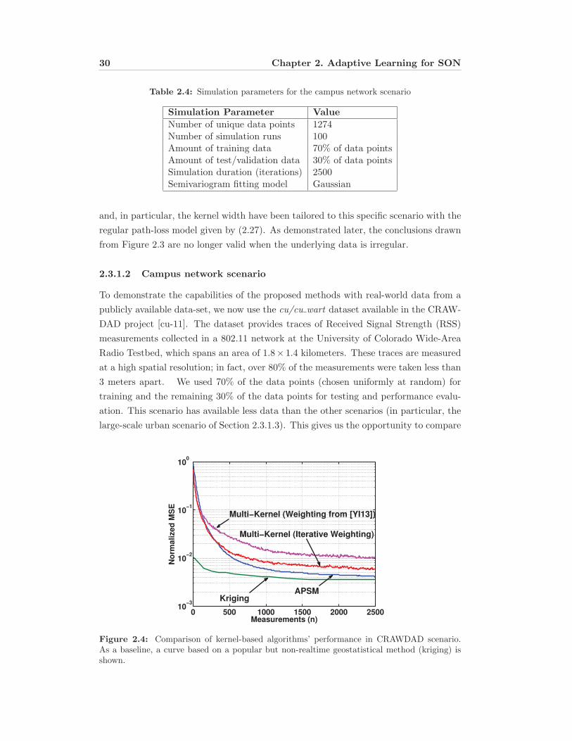
30 Chapter 2. Adaptive Learning for SON
Table 2.4: Simulation parameters for the campus network scenario
Simulation Parameter Value
Number of unique data points 1274Number of simulation runs 100Amount of training data 70% of data pointsAmount of test/validation data 30% of data pointsSimulation duration (iterations) 2500Semivariogram fitting model Gaussian
and, in particular, the kernel width have been tailored to this specific scenario with the
regular path-loss model given by (2.27). As demonstrated later, the conclusions drawn
from Figure 2.3 are no longer valid when the underlying data is irregular.
2.3.1.2 Campus network scenario
To demonstrate the capabilities of the proposed methods with real-world data from a
publicly available data-set, we now use the cu/cu wart dataset available in the CRAW-
DAD project [cu-11]. The dataset provides traces of Received Signal Strength (RSS)
measurements collected in a 802.11 network at the University of Colorado Wide-Area
Radio Testbed, which spans an area of 1.8× 1.4 kilometers. These traces are measured
at a high spatial resolution; in fact, over 80% of the measurements were taken less than
3 meters apart. We used 70% of the data points (chosen uniformly at random) for
training and the remaining 30% of the data points for testing and performance evalu-
ation. This scenario has available less data than the other scenarios (in particular, the
large-scale urban scenario of Section 2.3.1.3). This gives us the opportunity to compare
0 500 1000 1500 2000 250010
−3
10−2
10−1
100
Measurements (n)
No
rmal
ized
MS
E
Multi−Kernel (Iterative Weighting)
KrigingAPSM
Multi−Kernel (Weighting from [YI13])
Figure 2.4: Comparison of kernel-based algorithms’ performance in CRAWDAD scenario.As a baseline, a curve based on a popular but non-realtime geostatistical method (kriging) isshown.

2.3. Applications 31
the performance of our low-complexity online methods with (more complex) state-of-
the-art batch-processing methods. With reduced data, numerical issues due to finite
precision do not arise. In particular, we choose a popular method from geostatistics
for comparison; namely, ordinary kriging [Ste99, Cre90]. For example, in [GEAF14],
this method was applied to the estimation of radio maps (in particular, Signal to Noise
Ratio (SNR) maps). In Appendix A, we provide a short introduction to the kriging
method.
Figure 2.4 illustrates the decay of the MSE for the APSM algorithm and the mul-
tikernel algorithm as the number of measurements increases. Thereby, the MSE is
calculated using only the test data points, which were not used in the learning pro-
cess. We note that both algorithms behave as desired; the MSE decreases fast with
the number of measurements. (Our methods perform only one iteration per measure-
ment due to their online nature, however, we may re-use training data points multiple
times. Therefore, the number of measurements in Figure 2.4 is larger then the number
of available training data points.) The multikernel approach seems to be outperformed
by the APSM algorithm with respect to the convergence speed in this scenario. As
demonstrated in Section 2.3.1.3, this result does not seem to hold when the underlying
data is more irregular.
Not only is the estimation quality important but also the complexity, which grows
fast with the amount of data and the number of kernels. Therefore, in order to reduce
the complexity, we proposed in Section 2.2.4 an iterative weighting scheme that exploits
sparsity of the multikernel algorithm. In addition to the comparison to APSM, Figure
2.4 indicates that our iterative weighting approach significantly outperforms that of
[YI13] with respect to the convergence speed.
So far, we have only compared the two proposed kernel-based online learning
schemes with each other. However, it is also of interest to compare the proposed
methods with state-of-the-art approaches in the literature. Therefore, Figure 2.4 also
includes the MSE performance of the kriging approach. We highlight that kriging is
essentially an offline scheme where all measurements have to be available beforehand,
so a comparison is difficult and not entirely fair. In order to make a direct comparison
possible, we apply the kriging technique at certain time instances with all (at those
points in time) available measurements. Despite providing highly precise results given
the amount of available measurements (see Figure 2.4), this method has a serious draw-
back, which is inherent to all batch methods: the computational complexity does not
scale, since it grows fast with the number of data points available. In fact, all calcula-
tions have to be carried out from scratch as soon as a new measurement arrives. We
apply an ordinary kriging estimator with a Gaussian semivariogram model. The most
important simulation parameters can also be found in Table 2.4. The reader is referred
to [GEAF14] for further details.
In Figure 2.4, we can observe that, naturally, the kriging scheme shows very good

32 Chapter 2. Adaptive Learning for SON
Table 2.5: Simulation parameters for the large-scale urban scenario
Simulation Parameter Value
Number of users 750, 1500Simulation duration [s] 5000Number of base stations 187, 20Size of simulation area 7500 m × 7500 mSize of pixel 50 m × 50 mMeasurement frequency λ 0.1Number of simulation runs 10
results even with few measurements, but from a certain point in time, more measure-
ments do not significantly improve the quality of estimation. Moreover, we observe that
our kernel-based schemes, after a sufficient number of measurements (i.e., iterations),
achieves almost the same level of accuracy, but at a much lower complexity and in an
online fashion. To be more precise, we note that the kriging method needs to solve
a dense system of linear equations in every iteration. This has a complexity of O(n3)
(with n being the number of available samples). In addition, to obtain the results in
Figure 2.4 a parametric semivariogram model needs to be fitted to the sample data (see
Appendix A for details) which is a (non-convex) problem of considerable complexity.
2.3.1.3 Large-scale urban scenario
To assess their performance in real-world, large-scale, cellular networks, we also eval-
uated the algorithms using a realistic collection of data for the city of Berlin. The
data was assembled within the European project MOMENTUM and it is available in
Extensible Markup Language (XML) at [MOM04]. The data sets, which include pixel-
based mobility models, have been created to meet the need for more realistic network
simulations.
To be more precise, we resorted to the available data set for an area of 150 × 150
pixels, each of size 50 m× 50 m. This area represents the inner city of Berlin. For each
pixel, there was path-loss data for 187 base stations. This data was generated by ray
tracing based on real terrain and building information. Since we only need a single
path-loss value for each location, each pixel is assigned to a single base station with the
lowest path-loss value. This so-called strongest server assignment (assuming all base
stations transmit with equal power) determines the geometrical shape of cells because
each user reports its measurement only to the assigned base station. Moreover, each
base station estimates only the path-loss of assigned users, which defines the coverage
area of this base station. Path-loss measurements are assumed to be reported by each
user according to a Poisson distribution.
As far as the mobility model is concerned, it is assumed that users move on trajec-
tories with randomly chosen start and end points along a real street grid. To produce

2.3. Applications 33
x1
x 2
50 100 150
20
40
60
80
100
120
140 70
80
90
100
110
120
(a) True path-loss map.
x1
x 2
50 100 150
20
40
60
80
100
120
140 70
80
90
100
110
120
(b) Estimated path-loss map.
Figure 2.5: Visualization of original and snapshot of online-learned path-loss map in urbanscenario. The colorbar indicates the path-loss value in dB.
realistic movement traces, we used the street data from OpenStreetMap [URL14] in
conjunction with the vehicular mobility simulator SUMO [BBEK11]. The trajectories
were calculated using duarouter, a routing tool that is part of the SUMO simulator.
This combination allows us to generate movement traces with realistic speed limits,
traffic lights, intersections, and other mobile users. Furthermore, the traces enable us
to perform long simulations over time intervals of several hours with standard proces-
sors. It is emphasized that since some roads are more frequently used than others, the
distribution of measurements over the area of interest is not uniform. As a result, the
quality of estimation is not uniform. Finally, note that the trajectory of the UOI is
also generated randomly using SUMO.
In the following, we study the estimation performance of the APSM algorithm and
the multikernel approach. The simulation parameters are given in Table 2.5. Figure
2.5 provides a first qualitative impression of the estimation capabilities of the proposed
algorithms. We compare the original path-loss matrix H (Figure 2.5a) to the estimated
path-loss matrix H (Figure 2.5b) produced by the APSM algorithm after 5000 s of sim-
ulated time. Although each base station only learns the path-losses in its respective
area of coverage, the figure shows the complete map for the sake of illustration. A
visual comparison of both figures reveals significant similarities between the estimated
and the original path-loss maps. The path-loss maps estimated by the base stations
can now be used to provide predictions of path-loss conditions to particular users in
the system. To confirm the first impression of good performance by Figure 2.5, we
examine the estimation results along a route generated by the SUMO software between
two arbitrary locations. Figure 2.6 illustrates the path-loss prediction for an exemplary
route. While the dashed-dotted blue and red lines represent a particular sample of the
predicted path-loss, obtained using APSM and the multikernel algorithm, respectively,
the solid green lines represent the mean of the predicted path-loss traces (calculated

34 Chapter 2. Adaptive Learning for SON
0 200 400 600 800 100085
90
95
100
105
110
115
120
125
130
Travel Time [s]
PL
[d
B]
Prediction sample mean
Predicted path−loss (sample)
True path−loss along user’s trajectory
(a) APSM based prediction
0 200 400 600 800 100085
90
95
100
105
110
115
120
125
130
Travel Time [s]
PL
[d
B]
True path−loss along user’s trajectory
Prediction sample mean
Predicted path−loss (sample)
(b) Multikernel-based prediction
Figure 2.6: Comparison of true path-loss experienced by UOI and path-loss predicted bykernel-based methods in urban scenario.
from 100 runs of the simulation). In addition, we depict twice the standard error of
the mean as shaded area around the mean, which is calculated for each time instance.
Figure 2.6 compares the true path-loss evolution along the route with the predicted
path-loss evolutions for the two algorithms. The results are promising since the esti-
mated path-loss values closely match the true ones. Furthermore the estimation results
are expected to improve for routes along frequently used roads due to the large number
of available measurements. For the sake of completeness, we additionally computed the
MSE to complement Figure 2.6. By taking into account only the pixels that belong to
the specific route, we obtain a (normalized) MSE (as defined in (2.25) of 0.0037 for the
APSM algorithm and 0.0027 for the multikernel algorithm.
Now we turn our attention to the question of how much time the algorithms require
0 500 100010
−4
10−3
10−2
10−1
100
Time [s]
No
rmal
ized
MS
E
APSM
Multi−Kernel
Figure 2.7: Comparison of the MSE performance in urban scenario.

2.3. Applications 35
0 0.1 0.2 0.3 0.4 0.510
−3
10−2
10−1
100
Relative Error
No
rmal
ized
MS
E
APSM
Multi−Kernel
(a) Sensitiveness against errors in reported loca-tions. The relative error is defined to be the max-imum possible error in the measured coordinates(in meter) divided by the total dimension of thearea (7500m).
0 0.1 0.2 0.3 0.4 0.510
−3
10−2
10−1
100
Relative Error
No
rmal
ized
MS
E
APSM
Multi−Kernel
(b) Sensitiveness against errors in path-loss mea-surements. The relative error is the ratio of themaximum possible error per path-loss measure-ment to the average path-loss value (averagedover the path-loss values of all pixels). Therebya relative error of 0.1 corresponds to a maximumpath-loss error of (roughly) 10 dB.
Figure 2.8: Impact of errors on the MSE performance in urban scenario. Error bars represent95% confidence intervals under the assumption that the sample average of the MSE after 5000 sis normally distributed.
for sufficiently accurate estimation. To this end, we studied the evolution of the MSE
over time. One result of this study is presented in Figure 2.7, where we observe a
fast decrease of the MSE for both algorithms. The multikernel algorithm, however,
outperforms APSM, in terms of the MSE, with only a negligible loss in convergence
speed. This is in contrast to the observation made in the Rural or the Campus scenario.
We see two reasons for this changing behavior. Both are related to the fact that the
data, e.g., of the Campus scenario is more regular than that of the Berlin scenario.
The path-loss does not have sudden spatial changes. In this case, it is easier to tailor
the parameters of the APSM method, and, in particular, the kernel width to the data
at hand. In fact, with highly irregular data, a very narrow kernel is needed by the
APSM to achieve good performance, which is detrimental to the convergence speed.
In contrast, the multi-kernel algorithm has the advantage of offering multiple different
kernels to adapt automatically to the data, without manual tuning of parameters.
The measured value and the reported location can be erroneous. Therefore, it is
essential for the algorithms to be robust against measurement errors. Figures 2.8a and
2.8b depict the impact of incorrect location reports and erroneous path-loss measure-
ments on the MSE, respectively. This errors are chosen uniformly at random, with
a variable maximum absolute value that is investigated in Figure 2.8. Note that a
location error of less than 5% means an offset in each reported coordinate of at most
375 m (i.e., up to 8 pixels). Such large errors are usually not encountered in modern
GPS devices. From these simulations, we can conclude that both algorithms are robust

36 Chapter 2. Adaptive Learning for SON
0 1 2 3 4x 10
5
0
200
400
600
800
1000
1200
Measurement (n)
Dic
tio
nar
y S
ize
APSM
Multi−Kernel
Figure 2.9: Comparison of dictionary sizes using APSM and multikernel approach (withiterative weighting).
to the relevant range of errors but they are more sensitive to path-loss measurement
errors than to inaccurate location reports. In general, we can say that the multikernel
algorithm is more robust than the APSM algorithm. Finally, we show that the multik-
ernel algorithm, using our proposed iterative weighting approach, achieves an accuracy
similar to that of the APSM algorithm using a drastically smaller dictionary. This
can be concluded from Figure 2.9. For an exemplary simulation run, it shows that the
evolution of the dictionary sizes over time for the APSM algorithm and the multikernel
algorithm. We observe that the dictionary size of the multikernel algorithm is even
decreasing with the time, which is due to the block sparsity enforced by the second
term in the cost function given by (2.10).
The parameters of the algorithms have been tailored to the scenario at hand to
obtain the best possible estimation results. This however raises the question of how
sensitive the estimation performance is to parameter changes. To provide insight into
this problem, we performed experiments for selected parameters. As far as the APSM
algorithm is concerned, the parameters are the tolerable error level ε in (2.4), the step
size μ of the update in (2.6), the measure of linear independency αsp (cf. [ST08, Section
5.3]), which is used for sparsification, and the kernel width σ of the Gaussian kernel in
(2.26). In case of the multikernel algorithm, we study the impact of the error level εMK
in (2.9), the step size η, and the sparsification criterion δ (defined in [YI13, Equation
9]). Inspired by the principle of 2k factorial design [LK00, Chapter 12], we chose for
each parameter a very low value, indicated by the subscript l, and a very high value,
Table 2.6: Parameter choice in Figure 2.10a.
Parameter εl,APSM εh,APSM μl μh αl αh σl σhValue 0.0001 0.9 0.1 1.99 0.001 0.9 0.0001 1

2.3. Applications 37
Table 2.7: Parameter choice in Figure 2.10b.
Parameter εl,MK εh,MK ηl ηh δl δhValue 0.0001 0.9 0.01 1.99 0.5 0.99999
indicated by the subscript h (the particular parameter values are given in Tables 2.6
and 2.7). Then the algorithms were evaluated with all the parameter choices and the
resulting estimation accuracy was compared to accuracy of the default choice.
The results are summarized in Figure 2.10. In particular, Figures 2.10a and 2.10b
show the influence of important design parameters on the APSM algorithm and the
multikernel algorithm, respectively. From these figures, we can conclude that the MSE
improves by choosing a very small μ (cf. Figure 2.10a). However, these performance
gains are in general achieved at the cost of a worse convergence speed, which is ignored
in Figure 2.10. This observation is a manifestation of the known tradeoff between
convergence speed versus steady-state performance of adaptive filters [Say03].
2.3.1.4 Heterogeneous network scenario
An important scenario that is currently being investigated in the context of 5G is that
of dense heterogeneous networks. A typical scenario for evaluation of such networks is
the Madrid grid scenario proposed by the European METIS project [MET13]. The
simulation area, which is depicted in Figure 2.11a, has the dimensions 387 m × 552 m
and features 15 buildings, a park, and a pedestrian area. To avoid border effects, a
wrap-around model is applied. We assume a single 3-sectorized macro base station and
12 pico base stations, placed according to Figure 2.11a. The most important scenario
specifications (and other simulation parameters) are summarized in Table 2.8.
−0.5
0
0.5
1
1.5
2
2.5
3
3.5
εl,APSM
εh,APSMμ
lμ
hα
lα
hσ
lσ
h
Rel
ativ
e C
han
ge
in A
vera
ge
MS
E(l
og
−sca
le)
(a) APSM
−0.5
0
0.5
1
1.5
2
2.5
3
3.5
εl,MK
εh,MK
ηl
ηh
δl
δh
Rel
ativ
e C
han
ge
in A
vera
ge
MS
E(l
og
−sca
le)
(b) Multi-kernel algorithm
Figure 2.10: Effect of the algorithm parameters on the MSE in urban scenario. For eachrelevant parameter, a very small value and a very large value are investigated.

38 Chapter 2. Adaptive Learning for SON
Table 2.8: Simulation parameters for the heterogeneous network scenario
Simulation Parameter Value
Transmit power of macro/pico base station 46 dBm / 30 dBmAntenna height of macro/pico base station 53 m / 10 mNumber of base stations (sectors) 3 (macro) , 12 (pico)Size of simulation area 387 m × 552 mSize of pixel (resolution of data) 3 m × 3 mPercentage of training/test data variableNumber of simulation runs 30
In the following, we present results obtained with a corresponding state-of-the-art
(path-loss) data set, which is publicly available online at [MET15], provided by METIS
for this scenario. More specifically, ray-tracing based path-loss data is provided for
the three-sectorized macro base-station located at height of 52, 5 m (red markers in
Figure 2.11a), and the 12 pico base-stations (orange markers in Figure 2.11a)) located
at heights of 10 m. The path-loss data is provided for three different receiver heights
(1st floor, 8th floor, 12th floor). The path-loss data has a granularity of 184×129 pixel,
i.e., each pixel has a resolution of 3 m × 3 m.
In the following simulations, we try to reconstruct path-loss maps using the ground
floor data of the METIS data set described above. The main simulation parameters are
summarized in Table 2.8. We consider for each pixel the “strongest server” among all
macro and pico base stations, determined by the received power. That is, we calculate
for each pixel i the product pjgij , where pj ∈ R is the transmit power of base station
j (as given in Table 2.8) and gij ∈ R is the path-loss between base station j and
pixel i. Doing so, we can generate a map of strongest server path-loss values for each
pixel, which is depicted in Figure 2.11b. Please note that, in contrast to the previously
investigated scenarios, the data provided in the METIS data set comprises negative
path-loss values (which therefore could be also called path-gains).
We divide the available data into a fraction τ of the available data, which will
constitute the training data set and a corresponding fraction 1−τ , which will constitute
the test data set. For example, a training data ration of τ = 0.6 means that 60% of the
total available data (chosen at random) is used as training data and the remaining 40%
as test data. We generate a sequence of measurements by taking uniformly random
distributed samples from the training data. The measurements are arriving sequentially
in a random order, and we evaluate the normalized MSE as performance metric, as
defined in (2.25), for all data points in the test set. The results are averaged over 30
simulation runs, and the MSE value of a particular simulation run is thereby calculated
after receiving the last training data sample.
To give a first visual impression on the prediction performance of the proposed al-
gorithm using the METIS data set, Figure 2.11 illustrates the simulation area (Figure
2.11a), the (strongest server) path-loss data (Figure 2.11b), and gives an exemplary

2.3. Applications 39
(a) Simulation sce-nario (source: METIS[MET13])
(b) True path-loss map (c) Estimated path-loss map(APSM)
Figure 2.11: Illustration of simulation area and path-loss data (original and prediction). Thecolorbars in (b) and (c) indicate the path-loss value in dB. In (a), the light gray, shaded, areasindicate buildings, the green area is a park, black areas are streets, and the dark gray areaindicates a pedestrian shopping street. Red markers in (a) indicate macro base station sectorantennas, while the orange circles indicate the locations of pico base stations.
path-loss map that was predicted by the APSM algorithm (Figure 2.11c) using a train-
ing data ratio of τ = 0.6. The figure shows the complete map for the sake of illustration,
although parts of the prediction can be carried out locally in each base station, wher-
ever the measurements of path-losses in the respective area of coverage are available. A
visual comparison reveals significant similarities between the estimated and the original
path-loss maps, using this recent comparatively high-resolution data set.
In the following, we compare the performances of the two kernel-based algorithms
(with configurations given in Tables 2.1 and 2.2) in terms of the normalized MSE, and
additionally include the performance of the same ordinary kriging algorithm that was
introduced and described in the Campus scenario (Section 2.3.1.2). First, we compare
the normalized MSE produced by the algorithms for different amounts of training data
under the assumptions that measurements are taken and reported without errors. The
results are depicted in Figure 2.12.
Figure 2.12a compares the MSE (calculated over different total amounts of training
data) produced by the APSM, the multi-kernel, and the kriging algorithms for the
error free case. As noted before, the kriging algorithm is a batch algorithm, while the
other two algorithms perform online prediction. Therefore, we can only compare the
performance once all measurements are received (while the APSM and multi-kernel
algorithms can provide a prediction at any time). As we observe in Figure 2.12a, the
kriging method outperforms the other two algorithms in the error-free case, which is,
however, no surprise since the kriging method is not designed to enforce data sparsity,

40 Chapter 2. Adaptive Learning for SON
0 0.1 0.2 0.3 0.4 0.5 0.610
−4
10−3
10−2
10−1
100
Ratio of Training Data
MS
E
Multi−Kernel
Kriging
APSM
(a) Normalized MSE over training data ratio
0 0.1 0.2 0.3 0.4 0.5 0.6 0.7 0.8 0.910
2
103
104
105
Ratio of Training Data
Nu
mb
er o
f M
easu
rem
ents
Use
d
Kriging
Multi−Kernel
APSM
(b) Used measurements (dictionary size) overtraining data ratio
Figure 2.12: Performance comparison of kernel-based algorithms in METIS dense urbanscenario (error-free case) in terms of the MSE and the number of measurements used in theestimation process. As a baseline, a performance curve generated using the kriging method isshown.
but can use all information that is available. This gain, however, comes at the cost of
significantly increased complexity and unfavorable scaling behavior due to its batch-
processing nature. This becomes more clear in Figure 2.12b, which depicts the actual
number of data points used in the prediction. This number is significantly smaller
using the APSM than in the kriging approach, which uses all available data. However,
the multikernel approach needs even less data and gets along with only a small frac-
tion compared to the kriging algorithm. The reason for this economical way of using
the available data is the sparsification approach (enhanced by the iterative weighting
method described in Section 2.2.4.2), which is an indispensable feature considering the
huge amounts of available measurements (and other data) in future dense networks.
0 0.1 0.2 0.3 0.4 0.5 0.610
−3
10−2
10−1
100
Ratio of Training Data
MS
E
Multi−Kernel
Kriging
APSM
(a) Error distribution 1 (fewer outliers)
0 0.1 0.2 0.3 0.4 0.5 0.610
−2
10−1
100
Ratio of Training Data
MS
E
Multi−Kernel
Kriging
APSM
(b) Error distribution 2 (frequent outliers)
Figure 2.13: Performance comparison of kernel-based algorithms in METIS dense urbanscenario (erroneous measurements). As a baseline, a performance curve generated using thekriging method is shown.

2.3. Applications 41
Another major advantage of the multikernel algorithm becomes apparent when we
carry out the same comparison as above in a scenario, where we assume that the
measurements are superimposed with some measurement error. Thereby we model
the error term in a realistic fashion that also includes the possibility of strong outliers
(e.g., in cases where the user generated measurements are made at locations of bad
coverage or at times of bad fading conditions). For this reason, we use the following
error distribution. We add a random measurement error term ey given by
ey =
⎧⎨⎩n1, with probability a, and
n2, with probability (1 − a),
to each measurement yn. Thus, the error is chosen from one of two different (log-)
normally distributed random variables n1 and n2, which have standard deviations of
5 dB and 65 dB, respectively. The results of the simulations with measurement errors
are depicted in Figure 2.13. We consider two scenarios, which differ in the frequency
of high-error outliers: error distribution 1 (shown in Figure 2.13a), with a = 0.99, and
error distribution 2 (shown in Figure 2.13b), with a = 0.8. In Figure 2.13, we observe
that in particular the multikernel algorithm shows a significantly higher robustness
to measurement errors than the kriging algorithm (in case of very high errors, the
kriging performance initially even decreases with additional measurements). While
the performance of the multi-kernel algorithm deteriorates only gently (in particular
comparing Figure 2.12a with Figure 2.13a), the performance of the kriging baseline
rapidly deteriorates. The high susceptibility of the kriging algorithm to outliers in the
data can be explained by the fact that, as described in greater detail in Appendix A,
the kriging approach is designed to minimize the MSE of the prediction error variance.
Moreover, the MSE is known to be highly sensitive to outliers in the data [CMA94].
In contrast, the behavior of the multi-kernel approach is highly desirable, because
robustness regarding errors in the reported data is one of the main design criteria for
practical online learning schemes.
Extension to coverage maps The concept of coverage maps is closely related to
the prediction of path-loss maps. In general, we define coverage in terms of the received
power compared to a certain threshold. More precisely, we say that a location with
coordinates xj belongs to the coverage area of base station i if for a given threshold
η ∈ R the following relation holds:
fi(xj)pmaxi ≥ η, (2.28)
where pmaxi ∈ R is the maximum transmit power of base station i, and fi(xj) is the
function describing the path-loss of base station i, evaluated at location xj . Obviously,
there is a strong connection between coverage and path-loss. Coverage maps can be,

42 Chapter 2. Adaptive Learning for SON
(a) Estimated path-loss of exemplary basestation
(b) Corresponding estimated coverage
Figure 2.14: Estimated path-loss and coverage maps (using a threshold of η = −110 dBm) ofan exemplary base station in the METIS dense urban scenario (depicted in Figure 2.11a). In(a), the colorbar indicates the negative path-loss in dB. In (b), areas of coverage are coloredblue, while areas of no coverage are colored red.
for example, used as a pre-processing stage to decrease the dimensionality of energy
optimization problems, where one of the objectives is to define user-base station as-
signments in order to free and shut-down as many base station as possible. The main
idea is to use these maps to discard impossible location to base station assignments.
To determine the coverage of a given location is straight-forward if a base station has
access to path-loss information, e.g., from previously estimated path-loss maps. Thus,
the above described path-loss estimation procedure can be easily used to determine
coverage maps, by using the estimated path-loss instead of the true path-loss in (2.28).
Figure 2.14 shows a coverage map (Figure 2.14b) for an exemplary base station (located
south of the park area) that was obtained based on an estimated path-loss map (shown
in Figure 2.14a) with respect to this base station. Thereby, we assume the full transmit
power according to Table 2.8, and we (arbitrarily) choose a threshold of η = −110. This
threshold can be adapted to the particular scenario and application under consideration.
In Figure 2.14b, areas of coverage are colored blue, while coverage holes are marked
red. It can be observed that coverage holes appear mainly inside of buildings (note that
the scenario layout is depicted in Figure 2.11a). Based on such information network
operators can carry out measures to avoid connectivity problems, e.g., by increasing
transmit power, or by deploying additional femto-cells inside of buildings. Since the
prediction of the underlying path-loss maps (and therefor also the estimation of coverage
maps) is carried out in an online fashion, problem detection and self-healing algorithms
based on such maps can be easily incorporated into autonomous SON procedures.

2.3. Applications 43
Figure 2.15: Illustration of the interference situation in the network. Red regions indicatehigh interference.
2.3.2 Interference Estimation With Application to Device-to-Device
Communications
As a further application of the proposed kernel-based online estimation techniques, we
consider the problem of online interference estimation in cellular networks. Knowledge
of interference maps can be exploited in many different ways. This holds particularly
for SON, for example, to enable efficient network adaptation and resource utilization
by detecting problematic areas in the network. To illustrate this concept, Figure 2.15
depicts a snapshot of the interference situation generated using the Berlin scenario sim-
ulation tool introduced in Section 2.3.1.3 (details on the simulations will be provided
further below). In the figure, red areas indicate a high average interference in a typical
urban area with high numbers of mobile users. Geographic interference information can
be highly relevant for the adaptive control of dense cellular networks. If the informa-
tion contained in this map is accessible by some SON controller, self-optimization and
self-configuration mechanisms can autonomously resolve such problematic areas, e.g.,
by power control or antenna tilt optimization algorithms. In this section, we investigate
the estimation of interference maps in cellular networks with additional D2D commu-
nications and we will apply the estimated interference maps for channel estimation of
network assisted D2D communications.
D2D communications is a promising networking paradigm and a key enabling
technology for next generation wireless networks. Suitably selected wireless devices
can establish direct communication links without the need to transmit via macro-cell
base stations or other network elements. Two principle modes can be distinguished:
infrastructure-free D2D and network-assisted D2D. Infrastructure-free D2D communi-
cations is no solution for general purpose wireless services; therefore, in particular in
the context of 5G, network-assisted D2D communications [FDM+12] receives increas-

44 Chapter 2. Adaptive Learning for SON
ing attention. Although D2D communications as an enhancement of cellular networks
(such as LTE/LTE-A) is being heavily discussed, currently, there is no standard for
network-assisted D2D communications. However, the D2D communication paradigm
is considered as part of 3GPP Release 12 [Eri13, 3GP14b], where it is also known as
proximity services.
In network-assisted D2D scenarios, certain users can establish independent com-
munication links among each other, in addition to ordinary cellular communications.
These links may suffer from interference that is caused by the cellular communica-
tions, and in the same way, the D2D links may also cause interference to cellular users.
Thus, D2D communications poses additional challenges that result from the lack of
global knowledge at D2D transmitters and receivers. To control this interference, to
guarantee a sufficient robustness in critical applications, and to avoid wasting avail-
able resources, a certain amount of channel knowledge at D2D transmitters is needed.
Moreover, D2D channel knowledge enables base stations to actively support D2D users,
e.g., by reducing the interference between cellular and D2D communication links.
Therefore, obtaining such estimates is considered a major challenge in D2D commu-
nications. On a conceptual level, measurement based approaches (in conjunction with
data accumulation at the base stations) have been considered mainly in the context of
resource allocation. For example, [JKR+09] investigates D2D resource allocation based
on direct measurements of the interference levels (caused by cellular users and base
stations). In the context of LTE/LTE-A networks, a D2D channel estimation based
on reference signals, similar to the demodulation reference signal (DMRS) in the LTE
uplink, is proposed [FDM+12]. However, direct measurements of D2D channels may
not always be possible. A proper design is needed to avoid frequency collisions between
D2D and neighbor-cell cellular reference signals. Such a design might turn out to be
infeasible in certain situations. In fact, channel measurements and reporting for all
D2D pairs, and cellular users in the same cell, may not scale well as the number of
D2D pairs in the cell increases [FDM+12]. Therefore, further below, we propose to
generate estimates of the channel conditions of D2D users based on the prior learning
of geographic interference maps.
Subsequently, we investigate the learning of interference maps in network-assisted
D2D scenarios using the kernel-based algorithms introduced in Section 2.2.
2.3.2.1 Online interference estimation
As we have done for the estimation of path-loss maps, we model the problem of in-
terference map estimation as a regression problem. More precisely, we try to estimate
a mapping from geographic coordinates to a corresponding interference value, which
can be interpreted as the average interference that a cellular or D2D user (typically)
experiences when he travels across this geographic location. To model the interference
estimation problem, we will use the same notation as before (introduced in Section 2.2).

2.3. Applications 45
The estimation of the interference maps is based on measurements (xn, yn) at times
n, where xn := xn + εx ∈ R2 is the estimated coordinate of the reporting user and
yn ∈ R is a noisy interference measurement at coordinate xn. We will provide more
details on the practical measurements and the interpretation of this interference value
further below in this section. The relation between yn and the coordinate xn is given by
(2.2), where f : R2 → R is the unknown function that we attempt to learn. Moreover,
εx and εy model errors in the reported location and the reported interference value,
respectively.
Again, we are mainly interested in learning the interference at a discrete set of
locations (pixels). Therefore, we define
V ∈ RX1×X2 ,
to be the interference matrix (where, X1, X2 ∈ N specify the spatial extent of the
simulation area), which is composed of the values of the unknown interference mapping
function f evaluated at a given discrete set of locations. Each element of the matrix V
can be understood as the average aggregated interference at the corresponding location
(pixel). At each time instance, the base stations maintain an estimate V (based on the
current estimate of f) of the true interference mapping V , and this estimate is updated
whenever new measurements arrive.
At the user side, information that is readily available in current LTE networks can
be used to measure the interference, such as Received Signal Strength Indicator (RSSI)
measurements [3GP14c]. In LTE, the RSSI information is the total power that a user
observes across the whole band, containing not only power from the own (serving)
base station, but also power from other other cells (plus noise). It can therefore be
used as an estimate of the overall interference. Both the APSM-based algorithm and
the multi-kernel approach are suitable for the interference estimation task (a thorough
comparison between the two methods has been carried out in Section 2.3.1); in this
section, we use the APSM as a basis for the proposed algorithm, using the configuration
provided in Table 2.1 (except the kernel width parameter, which is specified further
below).
To demonstrate the performance of the resulting interference estimation method,
we carry out numerical simulations using the Berlin simulation environment that was
introduced in Section 2.3.1.3. The main simulation parameters are summarized in
Table 2.9. We use the already introduced SUMO simulator [BBEK11] (cf. Section
2.3.1.3) to generate movement traces based on an actual street map of the city center
of Berlin (from the OpenStreetMap project [URL14]), to obtain realistic movements of
vehicular users (at realistic velocities between 0 and 50 km/h). We consider a simulation
area of 7.5 km × 7.5 km, with 75 (macro-) base stations distributed in this area, and a
total number of 750 vehicular users. We further assume an LTE-based system with a

46 Chapter 2. Adaptive Learning for SON
Figure 2.16: Screenshot of simulation environment used to evaluate the online interferenceestimation algorithm. D2D-users move along a street grid (left) and the corresponding inter-ference is illustrated (right). The red circles mark the positions of D2D transmitters, while theblue triangles mark the positions of cellular base stations.
carrier frequency of 2 GHz and with 5 MHz available for D2D communications (which
corresponds to 25 LTE resource blocks). Note that within a cell, this band is assumed
to be reserved exclusively for D2D, however, different cells may use different portions
of the total system spectrum for this purpose. The base station has a transmit power
of 40 dBm, while the vehicular users transmits at a power of 10 dBm. The simulations
are illustrated by Figure 2.16, where base stations are indicated by blue triangles in the
left side of Figure 2.16, and D2D users are indicated by red circles. On the right side
of Figure 2.16, we depict the aggregated interference at each point on the map. The
value at a given pixel, which is indicated by different colors, is thereby the interference
(both from other base stations than the serving base station, and from D2D users) that
a user associated to the strongest base station experiences at this point. Thereby, it
is assumed that all cellular base stations are fully loaded (thus, no frequency band is
idle).
In our simulations, the channel is modeled as a superposition of pathloss and shad-
owing effects. We assume that the pathloss can be calculated as [3GP06]
PL(d) = 128.1 + 37.6 · log(d),
where d denotes the distance (in km) between sender and receiver. In addition we
assume a log-normal distributed shadowing process as specified in Table 2.9. Cellular
users, not depicted in Figure 2.16, are assumed to deliver RSSI measurements on a
regular basis. For the sake of simplicity, the measurements are assumed to arrive
according to a Poisson distribution (with parameter λ = 0.1) in time with a uniform
randomly chosen location. Note that in practical LTE systems, such measurements are
provided at an even higher frequency, which will further improve the prediction.

2.3. Applications 47
Table 2.9: Simulation parameters (interference prediction)
Simulation Parameter Value
Distribution of (RSSI) measurements uniform randomSimulation duration (#measurements) 2000Number of base stations 75Size of simulation area 7500 m × 7500 mSize of pixel 50 m × 50 mMeasurement frequency λ 0.1Shadowing (std. dev.) log-normal (10 dB)Base station transmit power 40 dBmD2D user transmit power 10 dBm
The learning performance of APSM is depicted in Figure 2.17. Again, we evaluate
the normalized MSE, as defined in (2.25) (replacing H and H by the interference
matrix V and its estimate V , respectively), averaged over 70 simulation runs. To
obtain performance estimations independent of the reporting frequency, we depict the
MSE over the number of reported measurements. It can be observed that initially the
MSE decreases fast and already after roughly 200 to 500 measurements (depending on
the particular kernel function), a reasonable performance level is reached.
In Figure 2.17, using a practical example, we have the opportunity to highlight a
particular issue in the design of kernel-based learning algorithms that we mentioned
already in the previous Section 2.3.1: the choice of the kernel parameters. Here, we
investigate the choice of the kernel-width σ2 of the Gaussian kernel (2.26) that we use
in the APSM. We can observe a manifestation of a well-known fundamental tradeoff
in kernel adaptive filtering between the initial convergence speed and the accuracy of
0 500 1000 1500 200010
−3
10−2
10−1
100
Number of measurements
No
rmal
ized
MS
E
APSM, Kernel−Width: 0.001
APSM, Kernel−Width: 0.005
Figure 2.17: MSE between true interference matrix and approximation, using different kernelparameters.
48 Chapter 2. Adaptive Learning for SON
the prediction in the long term [Say03]. Although a smaller kernel-width leads to a
much higher accuracy after 2000 measurements, this accuracy is achieved at the cost
of an initially slower decrease of the MSE. Thus, in practical scenarios the prediction
accuracy after only a few measurements has to be balanced against the long-term
performance.
2.3.2.2 D2D channel estimation and adaptive video streaming
Let us now consider a particular application of the above described online interference
estimation techniques: the estimation of D2D users’ channel conditions at the base
stations. As of today, the application of kernel-based online learning techniques in this
context is yet unexplored. The general idea is that the base stations use the proposed
radio map estimation algorithms to learn a mapping from geographic locations to the
average interference at the corresponding location. Based on the estimated interference
maps, together with suitable reports from D2D receivers, such as total received power
reports, the base stations can derive estimates of the (average) channel conditions of
active D2D users. Moreover, we demonstrate how this channel estimates can be used
in a very particular use-case: the adaptation of D2D video streaming transmissions,
e.g., as part of a later described “see-through” use case.
In addition to the measurements used by the learning algorithm, for the estima-
tion of D2D channels, we additionally assume that base stations have access to total
received power reports from D2D receivers in the system (e.g., RSSI measurements in
LTE/LTE-A). We denote the total received report at time t from D2D receiver r as
γ(t,xs,xr) = pshsr(t) + V (t,xr). (2.29)
Although in (2.29) we use the time index t to emphasize the time-dependence of channel
gains and interference power, our method is designed to obtain estimates of average
channel gains (on the same time scale as the prediction of interference) rather than
to track the influence of fast fading. Moreover, xs ∈ R2 is the location of the D2D
transmitter, xr ∈ R2 is the location of the D2D receiver, ps ∈ R is the transmit power
of the D2D transmitter, and hsr(t) ∈ R is the channel gain between the communicating
D2D devices. Using (2.29), the base station can use the knowledge of V (t,xr) and ps
to obtain an estimate of hsr(t) by
hsr(t) =γ(t,xs,xr) − V (t,xr)
ps.
Compared to measurement based methods, a major advantage of the method is its high
scalability and the avoidance of issues such as reference signal collisions. Compared to
non channel-aware schemes (i.e., in scenarios where measurements of D2D channels
are infeasible), the D2D transmitter is able to adapt transmission parameters (trans-

2.3. Applications 49
Figure 2.18: Schematic illustration of see-through use-case.
mit powers, modulation and coding, application-dependent parameters such as video
coding, etc.) to the estimated channel.
In the following, we numerically investigate the proposed procedure in a D2D video
streaming scenario. The video streaming transmission enables the driver of the receiving
vehicle to “see through” a vision obstructing vehicle (e.g., bus, truck) that is driving
ahead of his vehicle. This is illustrated in Figure 2.18. Using the generated channel
estimates, the transmitter is able to adapt its transmission to estimated average channel
conditions in order to increase the robustness, or to reduce the playback delay.
To obtain a realistic simulation of the see-through video transmission, we use a
publicly available video trace of appropriate resolution (“Sony Demo”, available at
[Vid14]). The video parameters are summarized in Table 2.10. In this configuration,
the video has a duration of approximately 10 minutes and requires a bitrate of on
average 5.8 Mbps (the bitrate at a given point in time depends on the sizes of the
corresponding frames to be transmitted). Due to the time-critical nature of the see-
through application, we assume that frames cannot be buffered at the transmitter and
erroneous frames cannot be retransmitted. In case of missing frames, the receiver
simply repeats the last correctly received frame in order to achieve the required frame
rate.
We model the D2D channels according to specifications by the METIS project
[MET13] for the urban micro scenario. We consider both Line-of-Sight (LOS) and
Non-Line-of-Sight (NLOS) communication scenarios, where the NLOS case is modeled
by a 10 dB higher path-loss [MET13]. In practice, the type of vehicles and the posi-
Table 2.10: Video streaming parameters (see-through scenario)
Video Parameter Value
Video Resolution HD 1280 × 720Codec H.264/AVC High Profile (VBR)Frames-per-second (FPS) 30Frame compression ratio 57.17Mean frame size 24181.9 bytesGoP-Size 12 (G12B2)No. of frames 17680

50 Chapter 2. Adaptive Learning for SON
tion of antennas, etc., determine whether LOS or NLOS propagation conditions are
predominant. All simulation parameters relevant for the “see-through” scenario are
summarized in Table 2.11. Based on our choice of simulation parameters, deducting
the control overhead, the maximum achievable transmission rate (using 64-QAM 3/4)
is 567 data bits per resource block, or 14.18 Mbps in total. Please note that the
Maximum Transmission Unit (MTU) is set to 1500 bytes. To render the simulation
tractable, we use a worst-case interference assumption, where the D2D transmission
suffers from interference from all (but the “serving”) base stations, and from all other
vehicular users (which are potential D2D users).
For the prediction part, we apply the APSM algorithm with the configuration de-
scribed in Section 2.3.2.1. Since the interference learning is a continuous process in-
dependent of the application, we can assume a certain “learning phase” before the
application starts, i.e., a certain knowledge about the interference situation already
exists. In our simulations we assume a learning phase of 10000 iterations of the APSM
prior to the D2D communication of interest.
In the following simulations, the channel-aware algorithm adapts the modulation
and coding scheme used for the video transmission (cf. Table 2.11) according to the
estimated (average) channel gain. As performance metrics we consider
1. frame error rates, and
2. the average playback delay per frame,
where we define the latter as the number of frame repetition events at the receiver
(caused by missing frames, which force the receiver to repeat the last correctly received
frame), multiplied by the frame duration (which is the reciprocal of the FPS value given
in Table 2.10), and divided by the total number of frames.
Moreover, we consider two baseline schemes for performance comparison. The first
base line is a static baseline, which transmits using a constant (pre-defined) Modulation
and Coding Scheme (MCS). Thereby, it chooses the minimum MCS that is able to
support the required average bit rate. The second baseline is an adaptive baseline, which
chooses the MCS according to instantaneous frame sizes, i.e., video bitrate demands
(but not according to the channel conditions). While the choice of MCS in the static
baseline does not change over time, the adaptive baseline chooses the minimum MCS
that theoretically allows a sufficiently high transmission rate in order to convey the
current block of video data. Given the current channel estimates, the channel-aware
scheme, however, can choose the maximum MCS (independent of the instantaneous
video transmission requirements) that allows to comply with a certain target Block
Error Rate (BLER). In the simulations, we use a target BLER of 0.1.
In Figure 2.19, we depict CDFs of the frame error rates (left) and the average delay
per frame (right), where only D2D transmissions are considered with communication
distances in the range between 7.5m and 25m (here, the LOS case is investigated). We

2.3. Applications 51
Table 2.11: Simulation parameters (see-through scenario)
Simulation Parameter Value
MCSs QPSK 1/2, QPSK 2/3, QPSK 3/4, 16-QAM1/2, 16-QAM 2/3, 64-QAM 1/2, 64-QAM 2/3,64-QAM 3/4
MTU 1500 bytesTarget BLER 0.1D2D distance 7.5m to 25mLearning phase 10000 iterationsMeasurement frequency λ 0.1
note that this range of distances is highly relevant for the considered “see-through” ap-
plication. Comparing the mean error produced by the adaptive learning-based scheme
to the mean error of the adaptive baseline, a reduction in the average frame error prob-
ability of around 35% is possible. Compared to the static baseline, the reduction is
around 18%, however, at the cost of a significantly worse delay performance. In fact,
we observe that the static baseline, which is only adapted to the average required video
rate, has a significantly worse delay performance than the other two approaches. When
the instantaneous channel conditions are good and the instantaneous rate requirements
are high (higher than the average video rate), resources are wasted since less data is
transmitted than possible and necessary. Although this leads to fewer frame errors
(a lower MCS is chosen than actually possible), it results in a high delay (number of
discarded frames) since not all of the 30 FPS can be transmitted. More frames are
discarded at the transmitter, since buffering is not possible. Moreover, the adaptive
baseline shows a higher frame error probability than the static baseline. This, however,
can be explained by the fact that the adaptive baseline adapts the transmission rate to
the instantaneous rate requirements (but not to the instantaneous channel conditions).
0 0.2 0.4 0.6 0.8 10
0.2
0.4
0.6
0.8
1
Relative Frequency of Frame Errors
cdf
Adaptive
Baseline
Static Baseline
(a) Frame error CDF
0 0.01 0.02 0.030
0.2
0.4
0.6
0.8
1
Average Delay per Frame [s]
cdf
Adaptive
Baseline
Static Baseline
(b) CDF of average delays per frame
Figure 2.19: CDFs of relative frequency of frame errors and average delay per frame in LOScase for communication distances between 7.5 m and 25 m.

52 Chapter 2. Adaptive Learning for SON
0 0.1 0.2 0.3 0.4 0.5 0.6 0.7 0.8 0.9 10
0.1
0.2
0.3
0.4
0.5
0.6
0.7
0.8
0.9
1
Relative Frequency of Frame Errors
cdf
Adaptive
Baseline
Static Baseline
LOS − case
NLOS − case
Figure 2.20: CDF of relative frequency of frame errors for a communication distance of 10 m.Comparison between the LOS case and the NLOS case.
When the instantaneous channel conditions are insufficient, but large frames have to
be transmitted (i.e., the adaptive baseline chooses a high MCS in contrast to the static
baseline), a larger number of frame errors occur.
In Figure 2.20, we compare the LOS and the NLOS case in terms of frame error
rates for a fixed communication distance of 10 m. In the NLOS scenario, a reduction
in the mean frame error rate of 30% can be achieved.
Note that in the numerical experiments described above we are primarily interested
in relative gains. For practical purposes, the frame error rates in Figures 2.19 and 2.20
may still be too large, in particular for the NLOS case. This results from the fact that,
in practice, the transmitter would not only adapt its MCS to the channel, but also the
video source coding rate, while in our simulations, we assume the video is encoded at
a constant rate (for high quality) as specified in Table 2.10.
2.3.3 Discussion
In all the different fields of applications that were considered in this chapter, we ob-
served that kernel-based adaptive filters are a promising tool for the design of adaptive
learning algorithms in wireless networks. As numerical results confirm, the proposed
methods fulfill important requirements for the usage in SON mechanisms, e.g., high
convergence speed, and robustness with respect to errors in the measurement data
and with respect to a non-uniform spatial distribution of measurements. Moreover,
considering the results of numerical experiments with different data sets lead us to
the conclusion that their prediction accuracy is largely independent of the resolution
of the underlying data. Furthermore, compared to state-of-the-art batch processing
algorithms (such as kriging), updates are made fast in an online nature and the incor-
porated sparsification mechanisms further reduce their complexity. Another advantage

2.3. Applications 53
is that side information can be easily incorporated to increase the prediction accuracy.
The estimated radio maps can be a valuable tool in all areas of SON. This includes
self-optimization approaches such as mobility management, load balancing, or direct
network topology adaptation. A reliable reconstruction of radio maps will also enable
future networks to better utilize scarce wireless resources and improve the QoS experi-
enced by the users. Moreover, radio maps are required in self-configuration and network
planning algorithms, since future cellular networks will have to be deployed with much
less a-priori planning than today, and without expensive measurement campaigns and
drive tests. Eventually, interference maps and similar radio maps, which can point
towards critical areas in the network, can be also valuable ingredients to self-healing
functions.
Beyond their direct application in SON, specifically the path-loss estimation is a
key ingredient in the reconstruction of coverage maps, which can provide a basis for
the development of proactive resource allocation schemes. Here, resource allocation
decisions are made, not only based on present channel state information, but also
based on information about future propagation conditions. In particular, the quality
of service experienced by mobile users can be significantly enhanced if the information
about future path-loss propagation conditions along the users’ routes is utilized for
proactive resource allocation. Possible applications of proactive resource allocation
are:
1. Anticipatory buffering: Assure smooth media streaming by filling the playout
buffer before a mobile user reaches a poorly covered area.
2. Anticipatory handover: Avoid handover failures by including a coverage map in
the decision-making process.
3. Anticipatory traffic offloading: Reduce cellular traffic load by postponing trans-
mission of a user until it has reached an area covered by Wireless Local Area
Network (WLAN) technology.


Chapter 3
Self-Optimizing Resource
Allocation in
Interference-Limited Networks
While the previous chapter was concerned with techniques to generate the required
system-wide knowledge for SON algorithms, in this chapter, we consider particular
self-optimization techniques for interference limited cellular networks.
As mentioned before, interference management in cellular networks is a crucial
SON mechanism [LPGD+11, AIIE12], especially in view of the trend towards dense
heterogeneous networks, since the particular dynamics of such networks render manual
configuration and optimization infeasible. Already state-of-the-art cellular networks,
such as LTE, are severely interference limited [BPG+09], not least due to increasing
bandwidth requirements by handheld devices with high data rate consumption. More-
over, next generation (5G) networks are expected to amplify the need for self-organizing
interference management even further [OBB+14].
At the same time, bandwidth has become an increasingly scarce resource. There-
fore, cellular networks experienced a paradigm change towards a frequency reuse of
one, which, consequently, increases the susceptibility of cellular users to interference.
Especially users at the cell-edge are affected by high Inter-Cell Interference (ICI).
This situation is further aggravated by the application of modern multiuser Multiple
Input Multiple Output (MIMO), also called SDMA, techniques in wireless networks.
SDMA allows to exploit the spatial distribution of users by using multiple transmit
antennas to transmit several downlink data streams on the same time-frequency re-
source. In addition to inter-cell interference, these schemes additionally suffer from
intra-cell interference (self interference). A potential solution to this problem are coordi-
nated transmission schemes, such as Coordinated Multi-Point (CoMP) in LTE [3GP13].
Such schemes can be divided into two categories: joint transmission, where neighbor-
ing base stations act as a large distributed antenna array, and coordinated schedul-
55

56 Chapter 3. Resource Allocation in Interference-Limited Networks
ing/beamforming. While, in theory, joint transmission schemes promise huge gains
[FKV06], they have high requirements on synchronization and backhaul bandwidth.
In fact, solutions to several challenges (such as reducing the costs of base station syn-
chronization, feedback compression and delay, handling of out-of-cluster interference,
efficient user selections, and many more) need to be resolved before the promised gains
from such schemes can be realized in practice [IDM+11]. Additionally, a centralized
control is difficult in the presence of multiple operator networks, small cells, and pos-
sibly privately operated femto-cells. As an alternative to fully coordinated schemes,
simpler SDMA schemes, with per-cell precoding and a certain level of coordination
have gained considerable attention [HAH09, BJ13].
There is a significant amount of research on coordination and interference mitigation
in cellular networks, for an overview the reader is referred to, e.g., [BPG+09, GHH+10].
A classical approach to avoid interference is to use a frequency reuse factor greater
than one, i.e., to assign different subbands of the available bandwidth to adjacent
cells based on a particular pattern. This, however, significantly limits the amount
of bandwidth available in each cell, which is undesired in current and future cellular
networks, owing to the scarcity of bandwidth. A straightforward extension of the
frequency reuse concept are fractional frequency reuse schemes [NGGA11], where the
available bandwidth is partitioned into regions with different reuse factors, e.g., for
cell-edge and cell-center users. In current frequency reuse-1 networks, interference
mitigation by power control and suitable resource allocation becomes inevitable.
There have been a variety of suggestions for joint multicell power control and
scheduling in cellular OFDM(A) based networks, such as the work in [GKGI07, HSAB09,
VPW09]. Recently, also multi-antenna systems have been considered; for example,
[YKS13], which investigates multicell coordination via joint scheduling, beamforming,
and power adaptation. Other directions include interference pricing and game theo-
retic approaches [SSB+09, YKS13, MHLT11]. It is commonly accepted that the un-
derlying joint optimization problems, which are non-convex in general, can be solved
optimally only for a limited set of problems and utilities in reasonable time. While
sub-optimal successive approximation techniques have become a popular tool to tackle
this non-convexity [PDE08, PE09], globally optimal solutions are often investigated
using branch-and-bound-based approaches [SLC08, JWCLA12, ASW12] or monotonic
optimization [UB12], however at a high computational complexity. Due to the large sig-
nalling overhead of centralized approaches, distributed coordination schemes in cellular
networks have gained increasing popularity [SLYC11, SV09, VPW09].
However, a distributed implementation, which is a well investigated aspect (as in
many of the aforementioned references), is not the only requirement. To be used in
current (and next generation) cellular networks, interference management schemes for
multiuser MIMO systems need to be dynamic (e.g., to cope with mobile users and
varying propagation conditions) and self-optimizing, in the sense that no-prior planning

3.1. System Model 57
or human interaction is required. Moreover, fairness among users (often enforced by
concave utility functions of user rates) has to be an integral component.
In this chapter, we aim to establish distributed and autonomous (in the sense that
no human interaction is necessary) interference management schemes for multi-antenna
cellular networks, which exploit the freedom in terms of resource and power allocation
offered by SDMA. Our algorithms jointly consider adaptive power control and suitable
resource allocation to users, and they are are built upon, and significantly extend ideas
presented in [SV09] for Single Input Single Output (SISO) networks. We evaluate
and compare our algorithms using a sophisticated LTE-based system-level simulation
platform, capable of mapping a high system complexity and investigating large network
sizes.
3.1 System Model
We consider the downlink of an LTE-like cellular network based on the concept of Or-
thogonal Frequency Division Multiple Access (OFDMA). (See, e.g., [STB09, GZAM10]
for a summary on OFDM/OFDMA in the context of LTE/LTE-A.) Each cell is sub-
divided into three sectors; in total, our cellular network is partitioned into M sectors
m ∈ {1, . . . ,M}. We assume base stations are equipped with nT transmit antennas
and in total there are I single-antenna users randomly distributed throughout the sys-
tem. Let Im be the number of users associated to Sector m. In the following, we adopt
some terminology from 3GPP LTE specifications. In particular, we assume slotted time
with time slots t ∈ Z+, which we call Transmission Time Interval (TTI). Moreover,
OFDM sub-carriers are grouped into J sub-bands, which we call Physical Resource
Block (PRB)s. Each PRB has a total length of 1 TTI in time.
While we use the term “base station” to refer to the entity that governs operations in
an entire cell, we use the term sector controller to refer to the entity that is responsible
for user selection and resource allocation in a particular sector. The (non-trivial) task of
each sector controller is to find scheduling decisions (being an assignment of available
resources on PRBs to users) and suitable power allocations that maximize a global
network utility function. Thereby, we employ a full-buffer traffic model where each
user has pending data at all times. Due to its simplicity this model is widely used for
performance evaluation of cellular networks in research and standardization [3GP10].
As mentioned before, we design interference management schemes for practical
SDMA networks. The concept of SDMA is illustrated in Figure 3.1. Users are separated
in the spatial dimension and parallel data streams can be transmitted to these users
by suitable precoding techniques. This allows to multiplex several users on the same
time-frequency resource. We assume a practical scheme, where the sector controllers
perform linear precoding and precoding vectors for beamforming are taken from a fixed

58 Chapter 3. Resource Allocation in Interference-Limited Networks
Figure 3.1: Conceptual illustration of spatial multiplexing (based on a geometric interpre-tation of beamforming). Parallel data streams can be transmitted to multiple users on thesame time-frequency resource by suitable precoding techniques. The parallel beams may causeintra-sector interference (indicated by the dashed lines).
N -element codebook
CN := {u1, ...,uN} ,
which is publicly known. Using fixed codebooks, SDMA can be realized with limited
feedback from the users [HAH09]. A popular scheme is Per User Unitary Rate Control
(PU2RC) [SE06], which uses orthogonal beamforming vectors; however, other codebook
designs with non-orthogonal beamforming vectors have been proposed as well [3GP07].
In this chapter, we will adopt the latter case and assume that users scheduled on the
same time-frequency resource may cause interference to each other. In the following,
we identify a beamforming vector ub ∈ CnT by its index b ∈ {1, ..., N}. The different
precoding vectors of the codebook are called ‘beams’ and can be used to simultaneously
support multiple users on the same time-frequency resource.
Using fixed codebooks is a practical assumption and allows us to compare our
algorithms with transmission schemes that are used in current MU-MIMO based cellular
systems [3GP11b]. From a sector controller’s perspective, this makes a beam b on
a specific PRB j a possible resource for user selection and power allocation. This
relationship is depicted schematically in Figure 3.2. In order to provide channel state
information to the sector controllers, users report feedback messages. This feedback
comprises a Channel Directional Information (CDI) and a Channel Quality Information
(CQI) value. The CDI value is a log2(N)-bit-value and signals the index of the preferred
precoding vector (beam) b∗, which is determined based on common pilot signals. The
CQI value reports the Signal to Interference and Noise Ratio (SINR) that the user
measured on the beam b∗, which is a (pilot-based) estimate of the users’ true SINR,
since scheduling decisions and resulting interference cannot be known in advance.
We allow resource allocation and power control to be carried out on a per-beam
granularity. Consequently, let pmjb ∈ R+ be the transmit power assigned to beam b on
PRB j in sector m. Moreover, let hmij (t) ∈ C
nT be the vector of instantaneous complex
channel gains from sector controller m to user i on PRB j. We assume frequency-flat

3.2. Network Utility Maximization 59
Figure 3.2: Resource grid from the scheduler’s perspective using a fixed transmit codebook. Ineach time slot, resource allocation and power control can be performed on a per-PRB-per-beamgranularity.
channels within a PRB. The noise power at the mobile terminals is denoted as σ2 ∈ R+.
For the duration of a time slot, the system is in a fixed fading state from a finite
set F . We denote by Pr{l} the probability of fading state l (with∑
l Pr{l} = 1).
Fading state l, in turn, induces a finite set of possible scheduling decisions K (l), i.e.,
assignments of available transmission resources to users.
3.2 Network Utility Maximization
We assume that the network operator tries to maximize a network-wide increasing
concave utility function
U(x) :=
M∑m=1
Um(xm), (3.1)
which is the sum of concave sector utility functions Um : RIm+ → R, defined over average
user rates xm ∈ RIm+ . Since we are obviously not interested in a specific ‘snapshot’ of
the system but in ergodic average rates, a possible control algorithm should not adapt
to a specific system state but should be able to optimize the system performance over
time.
Problem (3.1) can be decomposed in individual per-sector utility maximization
problems; the particular optimization problem for Sector m can be stated as
max.xm∈F
Um (xm) , (3.2)
where F ⊂ RIm+ is the convex and compact set of all possible average service rate vectors

60 Chapter 3. Resource Allocation in Interference-Limited Networks
(cf. [Sto05b]). The average rates can be modelled by the following constraints to (3.2):
xm ≤∑l
Pr{l}∑
k∈K(l)
φlmk rl (k) , (3.3)
∑k
φlmk = 1 (∀l,m). (3.4)
Thereby, Pr{l} denotes the probability of the system being in the particular fading state
l, and φlmk > 0 denotes the fraction of time slots that scheduling decision k is chosen,
provided the system is in fading state l. A scheduling decision is thereby a feasible
assignment of available (time/frequency/space) resources to users. More precisely, the
decision index k can be considered as an index of the (finite) set of all such assignments.
Furthermore, rl (k) ∈ RIm+ is the instantaneous rate vector comprising elements rli (k),
which represent the (sum-)rate that user i obtains when the system is in fading state l
and scheduling decision k is chosen.
Assuming an isolated sector with fixed powers and assuming stationarity and ergod-
icity of the fading process l(t), it is well-known that problem (3.2) can be asymptotically
solved by applying a gradient scheduler [Sto05b] at each time instance, without know-
ing the fading distribution. The gradient scheduler chooses the best scheduling decision
k∗ according to
k∗ (t) ∈ arg maxk∈K(l)
∇TUm (xm (t)) rl(t) (k) . (3.5)
Moreover, the gradient scheduler tracks average user rates xm (t) by updating them in
each time slot according to
xm (t + 1) = (1 − β) xm (t) + βrl(t) (k∗ (t)) , (3.6)
where the fixed parameter β > 0 determines the size of the averaging window. Please
note that in case logarithmic utilities are used (as in our numerical experiments), i.e.,
Um =
Im∑i=1
log(xmi ), (3.7)
the gradient scheduler is identical to the well-known proportional fair scheduler. Also
note that (as, e.g., in [SV09]) in case of OFDMA the gradient scheduler is simultane-
ously applied to each PRB. For a fixed power allocation (and assuming stationarity
and ergodicity of the fading process), the gradient scheduler is known to asymptotically
solve problem (3.2) [Sto05b] (i.e., the average rates xm converge to the optimal average
rates xmopt that solve (3.2)) for β → 0. Since, in this chapter, we consider multicell net-
works with dynamic power control, we cannot hope to find efficient and globally optimal
algorithms. However, we will present efficient schemes that increase the network-wide
utility in a distributed way by suitably assigning available time/frequency/space re-

3.3. Interference Mitigation by Autonomous Distributed Power Control 61
Virtual Model
Virtual Model
SectorController
SectorController
MessageExchange
Long-TermFeedback
Long-TermFeedback
Figure 3.3: General network control approach. Each sector controller maintains a virtualmodel of the network based on long-term feedback. Optimization in this model generatessensitivity messages, which are exchanged among sector controllers and which are used toadjust power allocations.
sources to users and controlling the transmit power budgets of the particular resources.
3.3 Interference Mitigation by Autonomous Distributed
Power Control
To tackle the problem of inter-cell and intra-cell interference we propose three different
self-organizing power control schemes based on long-term feedback from the mobiles.
Figure 3.3 depicts the general approach. The long-term feedback can be provided in
much larger intervals than the CDI/CQI short-term feedback described above. We note
that the assumption of such additional (infrequent) feedback reports is not far from
state-of-the-art cellular networks. Current standards, such as LTE-advanced, already
foresee advanced feedback concepts, where feedback reports are not even limited to the
serving base station [3GP13]. In addition to the long-term feedback reports of users, we
permit a limited message exchange between sectors. In the example of LTE networks,
this can be realized using the X2-interface [STB09, Section 2.6].
The proposed schemes are designed to pursue autonomous interference management
and to enable network entities to locally pursue the optimization of the global network
utility. The main difference between the three algorithms is the granularity of power
control.
• The first algorithm uses an opportunistic scheduler which only adapts power
62 Chapter 3. Resource Allocation in Interference-Limited Networks
budgets per frequency sub-band, which is then distributed equally among acti-
vated beams. We call this Opportunistic Algorithm (OA). It leaves full choice
to the actual scheduler as to which beam to activate at what time. The sched-
uler can therefore decide opportunistically. The power budgets per PRB, which
are equally distributed among activated beams, are determined by an associated
control procedure, which we will explicitly describe further below.
• The second algorithm is the Virtual Subband Algorithm (VSA), which enforces
the adherence to strict power budgets on each beam and consequently requires all
beams to be switched on at all times. The particular power values are derived by
a corresponding extended per-beam power control procedure. Having all beams
activated at all times has the advantage of making the interference predictable
when the power values are known. However, it leaves only limited freedom for the
actual scheduler, whose task is reduced to select a user for each beam. Since it
is always turned on, each beam (on each PRB) can be treated as an independent
resource for scheduling, just like a ‘virtual’ sub-band.
• The third algorithm is a hybrid approach, which permits opportunistic scheduling
at each time instance but, in addition, establishes average power budgets per
beam. We call it Cost-Based Algorithm (CBA). It leaves more freedom for
opportunistic scheduling than the virtual sub-band algorithm, which requires the
use of all beams at all times with strict power values. By contrast, CBA only
requires that target beam power values are kept on average. Instantaneously, the
scheduler is free to make opportunistic decisions based on its knowledge about
the current system state. In order to enforce that the power budgets are kept on
average, an additional cost term is introduced in the underlying utility function.
As we demonstrate later, the performance of the three algorithms is highly dependent
on the mobility assumptions on the users. In particular, we show that in scenarios
with high user mobility, it is more beneficial to impose average rather than strict power
budgets.
All proposed algorithms have the following general control procedure, or control
plane, in common. The control plane adapts power budgets using estimates of partial
derivatives of the network utility with respect to the power allocation of particular
resources. That is, estimates of the sensitivity of the network utility to changes of
the allocation strategies are generated. The particular allocation strategy can differ
between the algorithms. For example, the OA controls the power budget of an entire
PRB, while the VSA and the CBA control the power budgets of individual beams.
In all algorithms, the control plane is based on averaged, long-term, feedback of
users in order to avoid tracking fast-fading. The long-term feedback is used to calcu-
late corresponding virtual user rates and, in a second step, virtual average rates. The
virtual average rates do not have an immediate physical meaning in the ’real world’.

3.3. Autonomous Distributed Power Control 63
However, these rates are a good representation of the interference coupling throughout
the network and are used to calculate the ‘sensitivities’ to power changes on particular
resources both in the own sector and in other sectors. The sensitivity information is
compiled in messages and exchanged between the sectors. To reduce messaging over-
head, sector controllers could limit the message exchange to neighboring base stations.
Upon reception of the message vectors, the sector controllers calculate the desired esti-
mates of the system utility’s sensitivity to power changes on particular resources, and
adjust the power budgets accordingly.
Subsequently, we will focus on how the virtual average rates, which together form a
virtual model of the network, are calculated. In fact, besides the granularity of power
budgets, the derivation of the virtual model constitutes another main difference between
the proposed algorithms. In the following, we will discuss the particular algorithms in
greater detail.
3.3.1 Opportunistic Algorithm
OA is a direct extension of the Multisector Gradient (MGR) algorithm in [SV09] to
multi-antenna networks. Although OA is designed for SDMA networks, where multiple
users can be scheduled on the same PRB, it does not perform power control on a per-
beam basis (as opposed to the other two algorithms, which will be introduced in the
following two sub-sections). Instead, it controls the power budget per PRB. Moreover,
it allows the sector controllers to choose which beams to activate at every given time
instance.
As with any of the proposed algorithms, long-term feedback from users is required,
which in case of OA comprises long-term gains
gmij = maxb
⟨hmij ,ub
⟩, (3.8)
where hmij is the channel from user i to its sector controller on PRB j, averaged to
eliminate the influence of fast-fading. Moreover, a corresponding codebook index is
reported, which is the maximizing index b∗ in (3.8). Based on this feedback, the sector
controllers calculate a set of virtual user rates (the virtual model), which are used in
the process to derive the transmit power updates. In the following, in order to avoid
confusion with the instantaneous scheduling process outlined in Section 3.2, we denote
(wherever ambiguities occur) all virtual quantities using a tilde (∼). Let us define the
virtual user rates (time index omitted), given (virtual) scheduling decision k, by
rmij
(k)
= ρ(Fmij
),with Fm
ij :=gmij p
mj
(k)
σ2 +∑
m′ =m pm′
j gm′
ij
, (3.9)
with ρ : R → R being a function that maps SINRs to data rate, e.g., ρ(x) = log(1 +x).

64 Chapter 3. Resource Allocation in Interference-Limited Networks
Of course, if PRB j is not assigned to user i under k, rmij
(k)
= 0. Moreover, pmj
(k)
denotes the current power value of PRB j divided by the number of users scheduled
(hence also depending on the scheduling decision k), and pm′
j gm′
ij represents a long-term
estimate of the interference of sector m′ on PRB j.
Based on definition (3.9), the sector controllers can derive corresponding virtual
average user rates xm ∈ RIm . The sector controller can use these rates to obtain
estimates of the gradient of it’s local utility function with respect to power allocations
throughout the network (note that the utility function given in (3.2) is defined over
average user rates). Subsequently, these estimates (called sensitivities) are exchanged
in order to update the power budgets. In OA, the sensitivities are derived by virtual
scheduling (based on a similar procedure in [SV09]), which allows their computation
in an efficient and distributed way. Thereby, each sector continuously runs a (virtual)
gradient scheduler, which is known to locally maximize the sector utility. Similar to
the real scheduling process, the task to determine the virtual scheduling decision k
amounts to choosing the best subset of users to be scheduled on a PRB, subject to the
constraint that each user can only be scheduled exclusively on its reported beam (the
feedback scheme is explained in Section 3.1). We run the following gradient scheduling
steps nv times per TTI (in each sector m and for all J PRBs simultaneously).
1. Determine the virtual scheduling decision k∗ according to
k∗ ∈ arg maxk
∇TUm
(xm
(t
nv
))rj
(k,
t
nv
).
2. Update virtual average user rates according to
x
(t + 1
nv
)= (1 − β1) x
(t
nv
)+ β1J rj
(k∗,
t
nv
).
3. Update sensitivities according to
D(m,m)j
(t + 1
nv
)= (1 − β2)D
(m,m)j
(t
nv
)+ β2
Im∑i=1
∂Um (xm)
∂xmi
∂rmij
(k∗, t
nv
)∂pmj (t)
.
(3.10)
Thereby, β1 and β2 are small averaging parameters. Since the parameter nv determines
how long the virtual scheduler runs before accepting the sensitivities, a larger value
means more overhead by the virtual layer but a better approximation of average user
rates. Using (3.9), the derivatives in (3.10) are given by
∂rmij
∂pmj=
⎧⎪⎨⎪⎩
ρ′(Fmij
)Fmij
pmjm = m,
−ρ′(Fmij
)(Fm
ij )2
pmj
gmijgmij
m �= m.

3.3. Autonomous Distributed Power Control 65
The adaptation of the PRB powers can be summarized as follows. Starting with a
feasible power budget (e.g., equal powers), the sensitivities are occasionally exchanged.
Upon reception, the sensitivities are, for each PRB, summed up by each sector con-
troller. Each D(m,m)j in (3.10) is an estimation of the sensitivity of sector m’s utility to
a power change on PRB j in sector m. Consequently, the sum Dmj :=
∑Mm=1D
(m,m)j
gives an estimate of the network utility’s sensitivity to the power allocation on PRB
j in sector m. Subsequently, the power in each sector m is increased by some Δ > 0
on the PRB with the highest value of Dmj and decreased by Δ on the PRB with the
lowest value of Dmj (we will provide a more detailed description of the power adaptation
procedure within the following paragraph on VSA).
3.3.2 Virtual Subband Algorithm
Our second approach, VSA, allows power control on a per-beam granularity. As in
OA, the control plane of VSA that is responsible for determining the power budgets is
based on long-term Channel State Information (CSI). To this end, it requires long-term
feedback that comprises average link gains per beam and sector from each mobile. We
define
gmijb =∣∣∣⟨hm
ij ,ub
⟩∣∣∣2 (3.11)
to be the average link gain (the bar denotes empirical averaging over time) of mobile
terminal i on beam b and PRB j to sector controller m. Given average gains in (3.11),
each sector controller calculates corresponding virtual rates according to
rmijb = ρ(Fmijb), (3.12)
with
Fmijb =
gmijbpmjb
σ2 +∑
b′ =b gmijb′p
mjb′ +
∑m =m
∑b′′ p
mjb′′g
mijb′′
. (3.13)
Thereby, ρ : R → R denotes again the function that models the mapping of SINR to
data rate. Note that, since all beams are active at all times, we have an additional intra-
sector interference term (as opposed to the OA approach, where intra-sector interference
is assumed negligible by suitably choosing sub-sets of active beams, see also Section
3.4.2), which can no longer be eliminated by switching off beams. Based on the rates
in (3.12), the virtual average rates xmi of user i in sector m can be calculated as
xmi =
J∑j=1
N∑b=1
φmijbr
mijb. (3.14)

66 Chapter 3. Resource Allocation in Interference-Limited Networks
Here, φmijb ∈ [0, 1] represent optimal time fractions of resource usage for sector m. These
time fractions are determined as a solution to the optimization problem
f(r) := maxφmijb
∑i
Um
⎛⎝∑
j
∑b
φmijbr
mijb
⎞⎠, (3.15)
subject to∑
i φmijb = 1 and 0 ≤ φm
ijb ≤ 1 (for given virtual user rates r). We rely on an
explicit solution to (3.15) since, as the resources for scheduling (which are individual
beams here) are no longer orthogonal but cause interference to each other, we cannot
apply the virtual scheduling procedure proposed in [SV09] (as done, PRB-wise, by the
other two approaches). Based on the virtual user rates, the sector controllers calculate,
for all sectors (including self) and all beams, sensitivities to per-beam power changes,
which are given by
D(m,m)jb =
∑i
∂Um
∂xmi
∂xmi∂pmjb
=∑i
∂Um
∂xmi
∑b′
φmijb′
∂rmijb′
∂pmjb, (3.16)
where
∂rmijb′
∂pmjb=
⎧⎪⎪⎪⎪⎪⎪⎨⎪⎪⎪⎪⎪⎪⎩
ρ′(Fmijb′
) Fmijb′pmjb′
m = m, b′ = b,
−ρ′(Fmijb′
) (Fmijb′
)2
pmjb′
gmijbgmijb′
m = m, b′ �= b,
−ρ′(Fmijb′
) (Fmijb′
)2
pmjb′
gmijbgmijb′
m �= m.
The such generated sensitivities are exchanged in a regular, but not necessarily very
frequent manner between all sector controllers (depending on the availability of long-
term feedback (3.11) from users). Thereby, every sector m receives J · N sensitivity
values from all other (M−1) sectors, in addition to the J ·N values from its own sector.
Consequently, sector m calculates
Dmjb =
M∑m=1
D(m,m)jb , (3.17)
which can be either positive or negative. Since the particular Dm,mjb represent estimates
of the sector utilities to a power change on the resource jb in sector m, Dmjb clearly is an
estimate of the sensitivity of the system’s utility to a power change on the respective
beam. Based on these quantities, each sector can adjust its power allocation, thereby
steering the system operating point towards a greater utility in the virtual model.
The power adjustment is carried out in small fixed steps of Δ > 0. Let Pm(t)
denote the total allocated power in sector m at time t, and Pmax the upper bound on
the total sector powers. Then, the following procedure is applied.
1. Pick a virtual resource (jb)∗ (if there is one) such that D(m)(jb)∗ (t) is the smallest

3.3. Autonomous Distributed Power Control 67
among all virtual resources jb with D(m)jb (t) < 0 and pmjb (t) > 0. Now, set
pm(jb)∗ (t + 1) = max{pm(jb)∗ (t) − Δ, 0
}.
2. If Pm (t) < Pmax, pick (jb)∗ (if there is one) such that D(m)(jb)∗ (t) is the largest
among those resources jb with D(m)jb (t) > 0. Set
pm(jb)∗ (t + 1) = pm(jb)∗ (t) + min {Δ, Pmax − Pm (t)} .
3. If Pm (t) = Pmax and maxjbD(m)jb (t) > 0, pick a pair ((jb)∗, (jb)∗) (if there is
one) such that D(m)(jb)∗ (t) is the largest, and D
(m)(jb)∗ (t) is the smallest among those
virtual resources jb with pmjb (t) > 0 and D(m)(jb)∗ (t) < D
(m)(jb)∗ (t). Set
pm(jb)∗ (t + 1) = max{pm(jb)∗ (t) − Δ, 0
}, and
pm(jb)∗ (t + 1) = pm(jb)∗ (t) + min{
Δ, pm(jb)∗ (t)}.
Obviously, the algorithm reallocates power to beams with a large positive sum of sensi-
tivities. Note that, for numerical reasons, it may be necessary to specify a small positive
minimum power value per beam instead of allowing beam powers to be reduced to zero.
In this case, the changes to the algorithmic notation above are straight forward, so we
do not explicitly state them here.
3.3.3 Cost-Based Algorithm
The policy implemented by the VSA that requires the compliance with strict power
budgets per beam is very restrictive. The CBA is designed to enforce power budgets on
average, which instantaneously leaves a certain freedom for opportunistic scheduling.
This leads to the non-trivial problem of how to take average power budgets into account
in the scheduling process. For this, unlike the other two approaches, CBA also changes
the operation of the actual instantaneous scheduling algorithm. More precisely, CBA
introduces the following additional constraint to the Network Utility Maximization
(NUM) problem (3.2):
∀j, b : pmjb ≥∑l
Pr{l}∑k
φlmk cjb
(k, pmj
). (3.18)
Thereby, the terms cjb
(k, pmj
)represent the power cost, or power consumption, of
beam b (on PRB j) given scheduling decision k and the total power budget of PRB j
given by pmj . We assume that each beam that is activated gets an equal share of the
available total PRB power pmj . Thus, if nj(k) is the number of beams that are activated

68 Chapter 3. Resource Allocation in Interference-Limited Networks
on PRB j if decision k is chosen, the ‘cost’ of activating beam b on PRB j becomes
cjb(k, pmj ) =
1
nj(k)pmj ,
with pmj =∑
b pmjb.
To solve problem (3.2) with constraints (3.3), (3.4), and (3.18), we also have to
modify the gradient scheduler (3.5)-(3.6). For each PRB j, the modified gradient
scheduler now chooses the scheduling decision k∗ at time t according to
k∗ ∈ arg maxk
[∇TUm (xm (t)) ·
∑b
rl(t)jb (k) −
∑b
λjb (t) cjb(k, pmj
)], (3.19)
where rl(t)jb (k) ∈ R
Im+ are the instantaneous rates of all users on PRB j and beam b in
sector m, given scheduling decision k and fading state l(t). Dual parameters λjb (t),
tracking the deviation of powers from the target power values on a particular beam,
are updated according to
λjb (t + 1) =[λjb (t) + β3
(cjb
(k∗, pmj
)− pmjb (t))]+
. (3.20)
Average user rates xm (t) are maintained and updated as in (3.6). We note that the
above algorithm is of similar structure to the well-known Greedy Primal Dual (GPD)
algorithm [Sto05a], however, with power budgets playing the role of queueing states.
Having discussed the changes to the instantaneous scheduler, we now focus our
attention on how to generate and adapt the average power budgets. For this, we
use a similar concept of a virtual control plane as in the before-presented algorithms.
However, also the virtual control plane differs, e.g., from VSA, where every beam
is switched on all the time. First, in contrast to VSA, CBA uses a similar virtual
scheduling approach as OA to calculate sensitivity values (however, here, on a per-
beam granularity). Second, since the virtual schedulers mimic the operation of the
actual schedulers, the virtual scheduler is able to instantaneously (i.e., in a particular
iteration) deviate from the current target power budgets. To enable the calculation
of derivatives of the virtual rates with respect to beam powers (which are needed in
(3.24)), we introduce scaling factors αmjb
(k)
, which scale target beam powers pmjb to
power ‘costs’ cmjb
(k)
, which are the power values per beam that are instantaneously
employed by the virtual scheduler. Thus, αmjb
(k)pmjb = cmjb
(k)
. Again, we denote
variables from the virtual scheduler with a tilde (∼), wherever necessary.
Given average gains per beam similar to VSA, defined in (3.11), the sector con-
trollers calculate (virtual) user rates given by
rmijb
(k)
= ρ(Fmijb(k)
), (3.21)

3.3. Autonomous Distributed Power Control 69
with
Fmijb(k) =
αmjb
(k)gmijbp
mjb
σ2 +∑
b′ =b αmjb′
(k)gmijb′ p
mjb′ +
∑m =m
∑b g
mijbpmjb
. (3.22)
Virtual average user rates are calculated by CBA as follows:
xmi =∑j
∑k
φmjk
∑b
rmijb(k). (3.23)
Again, φmjk
are optimal time fractions of resource usage for sector m. To determine the
virtual average rates (and implicitly the time fractions), the following virtual scheduling
process is applied. In each TTI, the virtual scheduler performs nv scheduling runs. In
each run, the following steps are carried out on each PRB j:
1. Determine the virtual scheduling decision k∗ similar to (3.19).
2. Update virtual average rates similar to (3.6).
3. Update the virtual average power costs for each beam b similar to (3.20).
4. Update sensitivities for each beam b and sector m (β2 > 0 small) according to
D(m,m)jb
(t + 1
nv
)= (1 − β2)D
(m,m)jb
(t
nv
)+ β2
Im∑i=1
∂Um (xm)
∂xmi
∑b′
∂rmijb′(k∗, t
nv
)∂pmjb (t)
.
(3.24)
Using (3.21) to (3.22), the derivatives in (3.24) are given by
∂rmijb′
∂pmjb=
⎧⎪⎪⎪⎪⎪⎪⎨⎪⎪⎪⎪⎪⎪⎩
ρ′(Fmijb′
) Fmijb′pmjb′
m = m, b′ = b
−ρ′(Fmijb′
) (Fmijb′
)2
pmjb′
gmijbαmjb
gmijb′α
mjb′
m = m, b′ �= b
−ρ′(Fmijb′
) (Fmijb′
)2
pmjb′
gmijbαmjb
gmijb′α
mjb′
m �= m
.
The power adaption is then carried out similar to the other algorithms. For each
resource, each sector m sums up the received sensitivity values D(m,m)jb from all sectors
according to (3.17) and increases the power level on the beam with the highest positive
value of Dmjb in (3.17) while decreasing the power level on the beam with the largest
|Dmjb| among those beams with Dm
jb < 0. However, CBA adapts only power budgets per
beam, not actually used beam powers.
To find out whether CBA really complies with the average power budgets, Figure 3.4
gives a sketch of power trajectories (generated using the simulation environment de-
scribed in Section 3.4). Thereby, we exponentially average instantaneously used powers
per beam with the same time constant used for scheduling and compare the result to
the target power values determined by the virtual model. The left side of Figure 3.4

70 Chapter 3. Resource Allocation in Interference-Limited Networks
0 1000 2000 30000
1
2
3
4
5
TTI
NormalizedPower
1600 1800 20000
5
0 1000 2000 30000
1
2
3
4
5
6
NormalizedPower
TTI
Figure 3.4: (Averaged) power trajectories of ‘real’ scheduler (left) and target powers givenby virtual model (right). The power allocations of four exemplary beams are compared. The‘zoom’ indicates the averaging of powers over time. The four curves (red, green, light blue, anddark blue) indicate the averaged per-beam powers over time of the beams (here, a codebookwith four entries was used) of an arbitrary chosen PRB, both for the ’real’ scheduler (left), andfor the virtual layer (right).
shows the averaged powers, as actually used by the ‘real’ scheduler, while the right
side shows the target power values determined by the virtual scheduling procedure.
Note that since scheduling is opportunistic, instantaneously, the power levels fluctuate
highly and beam powers can differ from the target values (or a beam can be completely
turned off). This is illustrated by the ‘zoomed-in image’ in Figure 3.4 (left), where
actual powers without averaging are shown. It turns out that on average, the power
budgets are kept remarkably well.
3.4 Performance Evaluation
In order to compare the performance of the three algorithms in a setting close to prac-
tice, we conduct system-level simulations based on an LTE-like configuration. We focus
on the applicability in different fading environments, comparing the overall performance
with respect to a network-wide utility function as well as the performance of cell-edge
users.
3.4.1 Simulation Configuration
We employ a grid of seven hexagonal cells, each comprising three sectors of 120◦. To
guarantee similar interference conditions in each sector, a wrap-around model is used
at the system borders. The inter-site distance is 500 m and the minimum base station

3.4. Performance Evaluation 71
Table 3.1: System-level simulation parameters (evaluation of distributed algorithms)
Parameter Value
Number of sectors (M) 21Total number of terminals (I) 105 to 315Mobile terminal velocity 0 km/h, 3 km/hNumber of PRBs (J) 8Number of beams (N) (coordination) 4Number of beams (N) (baseline) 8Base station antennas (nT) 4Number of terminal antennas (nR) 1Simulation duration 10, 000 TTIPower adaption step size (Δ) 0.5% of the initial powerTraffic model Full buffer
to user distance is 35 m. Users are distributed randomly over the whole area. For
example, in case of a total number of 210 users in the system, we obtain an average
of 10 users per sector; however, the actual number of users in the particular sectors
may differ. A detailed description of the applied precoding codebooks can be found in
[3GP07]. As channel model, we use the WINNER model [WIN05], Scenario C2 (urban
macro) with a distance-dependent path-loss component calculated according to
PL(d) = 128.1 + 37.6 log(d),
with d being the distance in km, and a shadowing component with 8 dB standard
deviation. Each base station is equipped with 4 antennas (with 12λ antenna spacing) and
the maximum transmit power per base station is 46 dBm. All simulations are performed
with realistic link adaptation based on Mutual Information Effective SINR Mapping
(MIESM) [BAS+05] and a target BLER of 30%; moreover, we use explicit modeling
of Hybrid Automatic Repeat Request (HARQ) using chase combining (see [GZAM10,
Chapter 7] for details). Available modulation and coding schemes are QPSK, 16-QAM,
and 64-QAM. For efficiency reasons, we simulate a smaller number of PRBs (we use
J = 8) than in a real-world system; however, the results are expected to scale to a
higher number of PRBs. The carrier frequency is set to 2 GHz. The most relevant
parameters for the subsequent simulations can be also found in Table 3.1.
3.4.2 Baseline Algorithm
As baseline, we use a non-coordinative scheduling algorithm called Greedy Beam Dis-
tance (GBD) algorithm, with a codebook size of N = 8. GBD requires feedback from
each user, comprising a CDI and a CQI value. Note that the CQI can only be an
estimate of a user’s SINR, since the scheduling decisions cannot be known in advance.
More precisely, it is calculated based on the assumption that the user is scheduled alone

72 Chapter 3. Resource Allocation in Interference-Limited Networks
on the respective PRB and with full power. Therefore, it does not contain intra-sector
interference and can only estimate the magnitude of the inter-sector interference. On
each PRB, the users are assigned to beams in a greedy manner by using their best
beams feedback (CDI) and are selected using a proportional fair scheduling algorithm
based on their CQI feedback. Thereby, a minimum beam distance has to be kept, in
order to minimize the interference between users scheduled on the same PRB. This
distance is based on a geometrical interpretation of beamforming; therefore, given a
user is scheduled on a certain beam, adjacent beams (up to a certain ‘distance’) are
blocked and users that reported one of those beams are excluded from the list of can-
didates for the respective PRB. We use a minimum distance of three, that is, assuming
an eight-beam codebook, at most three users can be scheduled on the same PRB. No
adaptive power allocation is performed: the power is distributed equally among the
PRBs, and further among the thereon scheduled users / activated beams.
3.4.3 Global Utility Versus Cell-Edge User Performance
As mentioned before, we use two essential performance metrics. First, since we maxi-
mize a proportional fair utility, we compare the geometric mean of average user rates, in
the following called Geometric Mean of Average Throughputs (GAT), as a measure of
the increase of the overall utility. Maximizing the GAT is equivalent to maximizing the
sum utility as given in (3.7), since the geometric mean of a set of rates is equal to the
exponential average of the logarithm of the rates: the sum of logarithms is maximized
precisely if the geometric mean is maximized. Second, the performance of cell-edge
users, which we measure by the 5% quantile of average user throughputs, is a natural
benchmark for each distributed interference coordination algorithm.
Figure 3.5 shows cell-edge user throughput over GAT of the evaluated algorithms in
a scenario with user mobility (and therefore with fast fading), while Figure 3.6 depicts
the simulation results in a setting without user mobility. A problem that arises with
increased mobility is that the (virtual) model lacks behind the actual network state.
Especially when the controllers are restricted to a gradual power adaption process on a
per-beam granularity, they might not always be able to fully exploit multiuser diversity.
Since the proposed algorithms put different emphasis on opportunistic scheduling in
power adaption and resource allocation decisions, they perform differently when facing
user mobility and fast fading.
We compare the three self-optimization schemes to the uncoordinated baseline de-
scribed above. The performance curves are generated using different average number
of users per sector. More precisely, from left to right, the markers of the particular
curves in the figure represent average numbers of 5, 8, 10, 12, and 15 users per sector
(corresponding to total numbers of 105, 168, 210, 252, and 315 users in the network,
respectively). Obviously, increasing values on the ordinate correspond to increased fair-
ness with respect to the 5% quantile metric; moreover, higher values on the abscissa

3.4. Performance Evaluation 73
0 200 400 600 800 1000 1200 1400 1600 1800 200040
60
80
100
120
140
160
180
200
220
GAT [bit/TTI]
5%−q
uan
tile
of
use
r th
rou
gh
pu
ts [
bit
/TT
I]
CBAVSAOANo Power Control
Figure 3.5: Cell-edge user throughput vs. GAT in a fading environment. The averagedcell-edge users’ throughputs vs. the geometric mean of users’ throughputs are plotted for afast-fading scenario with users moving at 3 km/h. The three proposed distributed algorithmsare compared with a baseline algorithm without coordination. For each algorithm, the totalnumber of users in the network is varied. In particular, the markers in the figure, from left toright, represent an average number of 5, 8, 10, 12, and 15 users per sector. This correspondsto a total number of 105, 168, 210, 252, and 315 users in the network, respectively.
correspond to a higher sum utility with respect to the GAT metric. In both figures, we
observe that a higher number of users leads to an increased sum utility (due to the mul-
tiuser diversity effect); however, the cell-edge users suffer from a reduced performance
in this case (due to an increased competition for resources).
In case of user mobility (Figure 3.5), we observe that the CBA clearly outperforms
the other algorithms. In fact, for every simulated user density, either the 5% fairness
(low user densities) or both metrics are improved (higher user densities). For example,
in the case of 210 users in the network (corresponding to the third marker on the curves
in Figure 3.5), the CBA algorithm improves the performance with respect to GAT by
about 10% and in cell-edge user throughput by more than 35%. It can also be observed
that the VSA algorithm works best at high user densities, while in case of only a few
users in the cell, the OA algorithm (which requires the least overhead with respect to
additional feedback and signaling) and even the no-power control baseline show a better
performance, at least with respect to the cell-edge performance. The decreased GAT
shown by VSA in the fading case is an effect of leaving no freedom to the schedulers
for opportunistic scheduling, but to strictly specify the powers to be used for all beams
and time instances.
Figure 3.6 depicts the simulation results in a setting without user mobility. We can
observe that the OA offers already quite high performance gains, both in terms of GAT
and in terms of cell-edge user throughput, although being the least complex algorithm
(since power control is carried out PRB-wise instead of beam-wise). However, the
performance is even further improved by the other two algorithms. VSA can improve
especially the gains of cell-edge users, for example, in the case of 210 users in the

74 Chapter 3. Resource Allocation in Interference-Limited Networks
0 500 1000 15000
20
40
60
80
100
120
140
160
180
200
GAT [bit/TTI]
5%−q
uan
tile
of
use
r th
rou
gh
pu
ts [
bit
/TT
I]
CBA
VSA
OA
No Power Control
Figure 3.6: Cell-edge user throughput vs. GAT in a static environment. The averaged cell-edge users’ throughputs vs. the geometric mean of users’ throughputs are plotted for a scenariowithout user mobility. Thereby, the proposed three distributed algorithms are compared witha baseline algorithm without coordination. For each algorithm, the total number of users inthe network is varied. In particular, the markers in the figure, from left to right, represent anaverage number of 5, 8, 10, 12, and 15 users per sector. This corresponds to a total number of105, 168, 210, 252, and 315 users in the network, respectively.
network to more than 200% compared with no-power control. CBA again shows the
best performance by significantly improving the global utility compared with VSA (and
even more compared with no-power control). Again, this gain increases with increasing
number of users in the network.
3.5 Global Optimality: A Branch-and-Bound Based So-
lution
The numerical evaluation above clearly shows a superior performance of the proposed
distributed algorithms when compared with the static-power baseline. However, the
underlying optimization problem is non-convex; therefore, the distributed algorithms
will most likely end up in a local maximum. Therefore, it is of utmost interest to assess
the performance of the distributed algorithms with respect to how much of the theo-
retically achievable performance gains by cooperation are actually realized. Therefore,
we will subsequently derive methods to compare their performances to the globally
optimal solution. However, in their numerical evaluation, we restrict the scenario to a
network with two PRBs, two sectors, and two users each, due to the high complexity
of finding a globally optimal solution.
To further simplify the subsequent analysis, we restrict ourselves to the SISO case,
which essentially reduces all algorithms to the MGR algorithm in [SV09]. Moreover,
let us define a system-wide power vector p ∈ R(J ·M)+ , containing the power allocations
for all PRBs in all sectors, and a system-wide vector of time-fractions φ ∈ R(I·J)+ ,

3.5. Global Optimality: A Branch-and-Bound Based Solution 75
containing the resource usage for all users and all PRBs in the system. In this case,
the optimization problem can be stated as
max.p,φ
M∑m=1
Im∑i=1
log
⎛⎝ J∑
j=1
φmij r
mij (p)
⎞⎠ (3.25)
s.t. ∀j,m :
Im∑i
φmij = 1 (3.26)
∀m :J∑j
pmj ≤ Pmax, (3.27)
with
rmij (p) = log
(1 +
gmij pmj
σ2 +∑
m′ =m gm′
ij pm′
j
). (3.28)
As mentioned before, (3.25)-(3.27) is a non-convex optimization problem. Moreover,
due to the joint optimization in time fractions φ and power values p, the complexity is
significantly increased compared to only optimizing powers. From now on we will relax
the equality constraint (3.26) and obtain
Im∑i=1
φmij ≤ 1 (∀m, j). (3.29)
This gives us the possibility to treat all parameter pairs in the same way.
To gain insight into the deviation from the optimal solution of (3.25) with con-
straints (3.27) and (3.29), we can compare the distributed algorithm’s solution in sim-
plified settings to Branch-and-Bound (BNB), which is a popular global optimization
technique. Given a certain tolerance ε (which provides a trade-off between convergence
speed and accuracy of the solution), BNB converges to an optimal solution of (3.25).
BNB creates a search tree, where at each node, an upper and a lower bound to
the problem are evaluated. Details can be found for example in [HPT00]; see also
[ASW12] for an application to sum-rate maximization. The particular variant that we
apply can be summarized as follows. The algorithm is based on constantly sub-dividing
the feasible parameter region (called branching) and for each node of the resulting tree
calculating upper and lower bounds to the objective function (bounding). The process of
creating a particular node’s children by branching the corresponding parameter region
is called expanding the node. Nodes with upper bounds below the (globally) best lower
bound found so far can be deleted from the search tree (pruning) and do not have to
be considered any further (since they obviously do not contain the global optimum).
For the ease of notation, we combine all parameters to our objective function (that
is, powers and time fractions) in a single vector x ∈ Rn+, with n = J · (M + I). We
assume, without loss of generality, that the maximum sum power available in each cell

76 Chapter 3. Resource Allocation in Interference-Limited Networks
in (3.27) is normalized to one. Let X (0) ⊂ Rn+ denote our initial parameter region.
This region, determined by constraints (3.27) and (3.29), forms a convex n-dimensional
polytope with V (0) ∈ Z > 0 extreme points (or vertices) {x(0)v }. We collect all extreme
points of the polytope X (0) in the corresponding set
V(0) = {x(0)1 , . . . , x
(0)
V (0)}.
As mentioned before, BNB builds a search-tree by constantly branching the feasible-
parameter region. Thus a node l of the tree is associated with a certain parameter
region X (l) (with associated vertices V(l)) as well as a lower bound and an upper bound
on the objective value.
Remark 3.1. The parameter region X (l) can be expressed solely based on V(l), since
a point in a convex polyhedron can be expressed as a convex combination of the corner
points of the polyhedron. Therefore, each x ∈ X (l) can be expressed by a set of λj ≥ 0
such that
x =
|V(l)|∑j
λjx(l)j ,
with x(l)j ∈ V(l), and
∑j λj = 1.
Given a search-order based on a suitable search algorithm, the tree is traversed
node by node. Thereby the best lower bound among all nodes found so far, called
incumbent, has to be tracked. The parameters used to calculate the incumbent are
candidates for the optimal parameters. If the lower bound of a node is higher than the
current incumbent, it becomes the new global lower bound. If the upper bound of a
node l under inspection is lower than the incumbent, the optimal value can not be in
the associated parameter region X (l) and thus the node can be discarded (pruned).
In order to avoid infinite execution-time, a maximum difference ε between the real
optimum and the optimal value found by the algorithm is defined. If the upper bound
of a node is not more than ε above the highest lower bound, it is not further expanded
and the algorithm terminates when no further nodes have to be examined. Apart from
the value of ε and the quality of the bounds, the convergence speed is also heavily
influenced by the order of traversing the nodes of the tree. We use a best-first-search
in order to quickly obtain a good incumbent, to be able to prune as much nodes as
possible. That is, after expanding a node, we always choose the children with the
highest upper-bound next. If a node cannot be further expanded, the algorithm goes
up one level and proceeds with another child.
3.5.1 Bounding
Finding accurate and easy to compute upper and lower bounds is a crucial issue in the
design of BNB algorithms. Below, we explain how the upper and lower bounds to the

3.5. Global Optimality: A Branch-and-Bound Based Solution 77
sub-problems are found.
Let us begin with the upper bound. It is well-known [KTN12] that the (Shannon-)
rate expressions (3.28) can be written as a difference of concave (DC) functions (the
reader is referred to [HPT00, Chapter 4] for an introduction to DC functions and DC
programming) in the following way:
rmij (p) = log
(σ2 +
M∑m′=1
gm′
ij pm′
j
)︸ ︷︷ ︸
:=ζmij (p)
− log
⎛⎝σ2 +
∑m′ =m
gm′
ij pm′
j
⎞⎠
︸ ︷︷ ︸:=ηmij (p)
. (3.30)
Using (3.30), our non-concave objective function (3.25) can be rewritten as
M∑m=1
Im∑i=1
log
⎛⎝ J∑
j=1
φmij ζ
mij (p) − φm
ij ηmij (p)
⎞⎠ . (3.31)
Unfortunately, the function φmij ζ
mij (p) and also the function φm
ij ηmij (p) are neither convex
nor concave, since f(a, b) := a · log(1 + b) is not a concave function. However, we can
define the concave function(s)
ζmij (x) = φmij log
(σ2 +
1
φmij
M∑m′=1
gm′
ij pm′
j
),
and (in a similar same way) ηmij (x). Using this, (3.31) can be upper bounded by
M∑m=1
Im∑i=1
log
⎛⎝ J∑
j=1
ζmij (x) − ηmij (x)
⎞⎠ . (3.32)
Equation (3.32) is still not concave since it includes a sum of the concave function
ζmij (x) and the convex function −ηmij (x). To obtain a concave objective function, we
replace ηmij (x) by its convex envelope (cf. [HPT00]), defined as follows.
Definition 3.2. Let x1, . . . ,xV be the vertices of a polytope X . The convex envelope
γ(x) of a concave function g : X → R can be expressed as
γ(x) := minλ
V∑v=1
λvg(xv),
subject to∑V
v=1 λvxv = x, with∑V
v=1 λv = 1, and λv ≥ 0 (∀v).
Using this definition, the convex optimization problem that we have to solve in
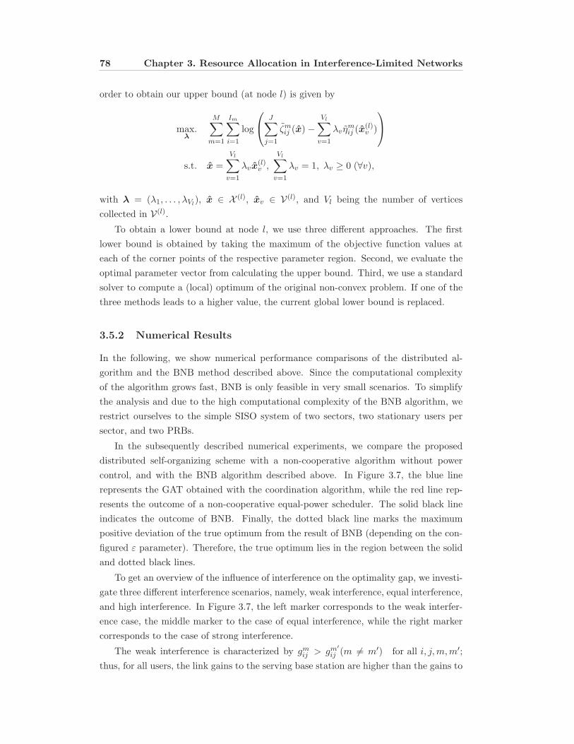
78 Chapter 3. Resource Allocation in Interference-Limited Networks
order to obtain our upper bound (at node l) is given by
max.λ
M∑m=1
Im∑i=1
log
⎛⎝ J∑
j=1
ζmij (x) −Vl∑v=1
λvηmij (x(l)
v )
⎞⎠
s.t. x =
Vl∑v=1
λvx(l)v ,
Vl∑v=1
λv = 1, λv ≥ 0 (∀v),
with λ = (λ1, . . . , λVl), x ∈ X (l), xv ∈ V(l), and Vl being the number of vertices
collected in V(l).
To obtain a lower bound at node l, we use three different approaches. The first
lower bound is obtained by taking the maximum of the objective function values at
each of the corner points of the respective parameter region. Second, we evaluate the
optimal parameter vector from calculating the upper bound. Third, we use a standard
solver to compute a (local) optimum of the original non-convex problem. If one of the
three methods leads to a higher value, the current global lower bound is replaced.
3.5.2 Numerical Results
In the following, we show numerical performance comparisons of the distributed al-
gorithm and the BNB method described above. Since the computational complexity
of the algorithm grows fast, BNB is only feasible in very small scenarios. To simplify
the analysis and due to the high computational complexity of the BNB algorithm, we
restrict ourselves to the simple SISO system of two sectors, two stationary users per
sector, and two PRBs.
In the subsequently described numerical experiments, we compare the proposed
distributed self-organizing scheme with a non-cooperative algorithm without power
control, and with the BNB algorithm described above. In Figure 3.7, the blue line
represents the GAT obtained with the coordination algorithm, while the red line rep-
resents the outcome of a non-cooperative equal-power scheduler. The solid black line
indicates the outcome of BNB. Finally, the dotted black line marks the maximum
positive deviation of the true optimum from the result of BNB (depending on the con-
figured ε parameter). Therefore, the true optimum lies in the region between the solid
and dotted black lines.
To get an overview of the influence of interference on the optimality gap, we investi-
gate three different interference scenarios, namely, weak interference, equal interference,
and high interference. In Figure 3.7, the left marker corresponds to the weak interfer-
ence case, the middle marker to the case of equal interference, while the right marker
corresponds to the case of strong interference.
The weak interference is characterized by gmij > gm′
ij (m �= m′) for all i, j,m,m′;thus, for all users, the link gains to the serving base station are higher than the gains to

3.6. Discussion 79
Weak Equal Strong−6
−4
−2
0
2
4
6
8
Interference Scenario
(Ave
rag
ed)
GA
T
Equal Power
Coordination
BnB−Result
BnB−Result+ε
Figure 3.7: Comparison of the distributed power control with BNB solution for differentinterference regimes.
the interfering base station. Note that this is, from a practical point of view, the more
interesting case since, e.g., due to handover algorithms, users are usually associated
to the strongest base station. It can be observed that the distributed power control
performs quite well since we see a significant improvement over equal power scheduling.
Moreover, in this case, the GAT of the distributed power control is closest to the BNB
algorithm.
In the ‘equal’ interference case, the gains to the interfering base stations are roughly
the same as the gains to the serving base station; thus, gmij ≈ gm′
ij (m �= m′), for all
i, j,m,m′. It can be observed that the gap of the cooperativ scheme to BNB is larger,
compared to the weak interference case, although it shows significant improvements
over non-cooperative scheduling.
The strong interference case is characterized by gmij < gm′
ij (m �= m′), for all i, j,m,m′;that is, for all users, the link gains to the interfering base stations are higher than the
gains to the serving base station. Here, the gap in the non-cooperative algorithm’s
performance, compared to the BNB result, is significantly larger than in the other sce-
narios. By contrast, the power control algorithm shows roughly the same performance
gap than in the case of equal gains.
3.6 Discussion
In this chapter, we proposed distributed algorithms for interference coordination in cel-
lular networks, which is a major field of application for SON. The proposed algorithms
achieve a (soft) fractional frequency reuse [BPG+09, SV09] in an autonomous, self-
organizing manner by allocating different power levels to different frequency subbands
and extend this concept to the spatial dimension in multi-antenna networks.
Numerical system-level evaluations indicate that the proposed algorithms are appli-
cable in practice and show significant gains over the uncoordinated case. In particular

80 Chapter 3. Resource Allocation in Interference-Limited Networks
for the CBA, these gains can be observed not only for cell-edge users but also in terms
of the network-wide utility. The simulations were carried out with an LTE parameter
set in order to show the applicability of the proposed methods for state-of-the art cellu-
lar networks. The results further motivate the use of considerably simpler distributed
coordinated beamforming and scheduling techniques as an alternative to complex joint
transmission schemes in multi-antenna networks. Furthermore, we can conclude that,
in particular when the users are mobile and fast-fading is considered, power budgets
should not be enforced strictly but rather on average, to instantaneously realize the full
multiuser diversity gains.
Although the network-wide power control is an intractable non-convex optimiza-
tion problems, the algorithms efficiently provide approximations to its solution, using
a virtual scheduling process based on long-term channel estimates. Comparisons to a
near-optimal branch-and-bound based solution show that, especially for practical in-
terference regimes, the self-organizing distributed algorithms significantly improve the
network’s operating point towards the optimal solution.

Chapter 4
Flexible Stochastic Network
Control
An implicit modeling assumption of the previous chapter is the so-called full buffer
assumption, i.e., there is an infinite amount of data to transmit for all users at all
times. This is a commonly made assumption, however, it masks some important issues
that arise in practical networks. In this chapter, we drop this idealized assumption and
consider stochastic traffic models, which allow to investigate additional characteristics
of wireless data networks, such as bursty arrivals of packets, idle times, and queueing
delays. Thereby, we do not restrict ourselves to the cellular networks paradigm, but
consider more general multi-hop network topologies. In such networks, self-organization
also plays a crucial role. In particular, new types of sensor networks, including smart
meters, direct D2D and machine-to-machine communications, but also particular re-
quirements from application layer data traffic induce the need for self-organization
capabilities. In the following, we assume that operations of the network, such as rate
allocations, traffic flow scheduling, and routing decisions, are determined by a control
policy, both on a global and on a local level. Adaptive control policies can support
self-optimization and self-configuration by adapting these operations, e.g., to varying
service requirements, queueing states, or battery levels.
We approach the design of control policies for wireless networks from a service
centric–or application centric–point of view. Thereby, we assume that the service layer
requirements can be expressed as constraints on buffer states. For example, a general
delay-sensitive application may require certain maximum levels of the buffer states,
while a multimedia streaming application will additionally need minimum buffer state
constraints at the user devices, such that the stream will not be interrupted due to
buffer underflows. While the first type of constraint is well investigated, the second
type bears serious challenges, especially in multihop networks.
When considering stochastic traffic models, it is of utmost interest to have control
policies that support as much data traffic as possible, while keeping the size of the data
81

82 Chapter 4. Flexible Stochastic Network Control
queues bounded. This property is also called throughput optimality (we will define this
more precisely further below). Following the seminal work of Tassiulas and Ephremides
[TE92], throughput optimal queueing control in stochastic networks, in particular the
throughput optimal MaxWeight policy, has gained considerable attention. A major
advantage of this algorithm is that it can perform resource allocation adaptively in
a self-organizing fashion, i.e., without prior planning. Despite its simplicity, its ap-
plication in practice turned out to be difficult, since it can lead to significant delays
[SL07]. Significant efforts followed on reducing the delay of MaxWeight-type policies
[BSS11, YSRL11]. A general class of throughput optimal policies with improved delay
performance was recently presented in [NZJ12].
However, delay is not the only relevant performance measure, in particular when
we consider modern multimedia applications. In fact, a policy that is designed to op-
timize only delay can be even harmful. Consider, e.g., the case where the receiver
buffers are strictly size-limited. Here, it can be better to absorb traffic peaks at inter-
mediate buffers instead of routing packets as fast as possible to the user. Moreover,
in cases where the application is satisfied with the offered performance, it is not nec-
essary to invest much in further incremental improvements of particular performance
measures. Therefore, a sophisticated control approach should be able to flexibly cope
with specific, possibly time-varying, requirements that are dictated by the actual appli-
cations (streaming services, gaming, etc.). Nevertheless, stability cannot be sacrificed.
Consider, for example, multimedia streaming traffic, which constitutes an ever larger
fraction of the traffic observed in nowadays wireless networks. Here, we have to ensure
that application buffers do not run empty, in order to avoid interrupting the playback
of the stream. This results in minimum buffer size constraints. However, it should be
also avoided that buffers grow too large (for example by transmitting content to the
user as fast as possible), since (1) buffers could be limited in size and (2) the user might
switch the video stream, which implies a waste of already invested resources.
While queueing networks with performance metrics, such as throughput [TE92],
delay [BSS11] (including deadline constrained traffic [LE12]), and fairness [Sto05b], are
well investigated in the literature, the problem of minimum buffer constraints was to
date mainly considered in the context of stochastic processing networks [HN11]. In the
domain of queueing networks, previous works consider underflow constraints in rather
simple network topologies, such as broadcast networks [MOHC10, SLW11]. For exam-
ple, in [MOHC10], the problem is investigated in a network of multiple transmitter-
receiver pairs with cooperating transmitters. The available resources per user are di-
vided into a fixed and a variable part; when the application buffer states are low, the
variable rate is increased, and decreased, when the application buffer states are high.
The approach in [MOHC10] requires that buffer levels for each user progress indepen-
dently of other users; therefore, it is limited to networks with broadcast or (multiple)
point to point links. It cannot easily be generalized to multihop networks (not even to

4.1. Preliminaries 83
the simple tandem network depicted in Figure 4.3).
Recently there has been some interest in queueing network control with an arbi-
trary underlying cost-metric [Mey08], allowing to incorporate application-dependent
constraints in the control policy. However, stability and cost performance crucially
depend on the parameter choice, which therefore has to be adapted in simulations.
In the following, we introduce a framework for the design of wireless queueing net-
work control policies with particular focus on combining stability with a cost function
based approach that provides the flexibility to incorporate constraints and requirements
of particular services or applications. Given the huge variety of different applications
and possible requirements on adaptive network control, we focus on a selected num-
ber of exemplary applications. In this respect, we consider the reduction of buffer
underflows in case of streaming traffic, and the maximization of idle times for energy
savings in networks of energy-constrained (e.g., battery powered) nodes. Moreover,
we demonstrate the application of our framework in cross-layer control problems for
wireless multihop networks. We compare various candidate cost functions and show
how the throughput optimality of corresponding policies can be verified using simple
conditions for stability. But first, let us introduce some important preliminaries.
4.1 Preliminaries
We begin with a brief summary of the concept of Markov chains, which provide pow-
erful means for the description and analysis of dynamic systems, and constitute the
basic theory for the concept of queueing networks. A discrete-time stochastic pro-
cess {q(t) : t ∈ Z+} with values in the countable state-space S is called (discrete-time)
Markov chain if only the present state contains information about future states, i.e,
Pr{q(t) = xt | q(t− 1) = xt−1, q(t− 2) = xt−2, . . .} = Pr{q(t) = xt | q(t− 1) = xt−1},
where all xj ∈ S. Knowledge about past states does not add any further information.
Let us define the transition matrix P of a Markov chain with countable state space as
[P ]x,y = Pr{q(t + 1) = y | q(t) = x}.
Applying this concept recursively, we can also define the t-step transition matrix
P t := PP t−1. An important concept is irreducibility, which, broadly speaking, im-
plies that all states of the Markov chain can be reached from any other state. In this
chapter, we consider the following definition.

84 Chapter 4. Flexible Stochastic Network Control
Definition 4.1. (cf. [Mey07, Chapter 8]) A Markov chain is said to be x∗-irreducible
if the given state x∗ ∈ S is reachable from each initial condition, i.e.,
∞∑t=0
[P t]x,x∗ > 0, ∀x ∈ S.
If the chain is x∗-irreducible for each x∗ ∈ S, the chain is simply called irreducible.
Using the first return time τx∗ to the fixed state x∗ ∈ S, the chain is positive recurrent
if and only if E{τx∗} < ∞ [Mey07, Theorem A.2.1].
4.1.1 Queueing Model
The simplest example of a queueing network is a single queue, which comprises a server
and jobs that queue up at the server until served. A job leaves the system when the
service is complete. Single queues are often described using Kendall’s notation [Ken51].
In short form, a description according to this notation is given by A/B/m, where A
denotes the distribution of the arrivals, B denotes the distribution of the service times,
and m denotes the number of servers. The simplest example is the G/G/1 queue, which
describes a single server system with general inputs and service times (or GI/G/1, if
the independence of inputs shall be emphasized). A popular example is the M/M/1
queue, which has a single server, and where the jobs arrive following a Poisson process
with intensity α, and the service times of the jobs are determined by independent
exponentially distributed random variables with rate μ. This model is useful to describe
the behavior of a single queue; however, we need models that are suitable for networks
of queues.
In order to describe communication networks based on the concept of queueing
networks, we resort to a simple, discrete time, stochastic network model, which is
called Controlled Random Walk (CRW) model. Subsequently, we summarize the main
elements of this model (a detailed exposition of this model is also given in [Mey07]).
Let us consider a single queue first. In this case, the model is defined by the process
q(t + 1) = q(t) − s(t + 1)u(t) + a(t + 1), t ∈ Z+.
The service rate and arrival rate sequences {s(t)}t≥0 and {a(t)}t≥0, respectively, are
assumed to be independent and identically distributed (i.i.d.), and the control sequence
{u(t)}t≥0 is confined by 0 ≤ u(t) ≤ 1.
In general, however, we consider a queueing network that consists of m ∈ Z queues
in total. These queues represent physical buffers (with potentially unlimited storage
capacity). Let M be the set of queue indices. We arrange the queue backlogs at time t
in the vector q(t) ∈ X , with q(t) = [q1(t), . . . , qm(t)]T , which we refer to as the queue
state. The space X can be equal to Zm+ , but also constraints, e.g., limits on buffer levels,
can be incorporated. As in [TE92, Nee10], we assume per-destination queueing; that is,

4.1. Preliminaries 85
αq1 q2 q3 q4
q5
Figure 4.1: Exemplary queueing network.
each node maintains a (logical) First In, First Out (FIFO) queue for each destination
in the network. As before, suppose that the evolution of the queueing system is time
slotted with t ∈ Z+. Then, our model is defined by the queueing law:
q (t + 1) = [q (t) + B (t + 1)u (t)]+ + a (t + 1) . (4.1)
In what follows, the queueing system (4.1) is assumed to be a x0-irreducible Markov
chain, where x0 corresponds to the empty system state (i.e., x0 = 0). The vector
process a (t) ∈ Zm+ is the (exogenous) influx to the queueing system with mean α ∈ R
m+ .
That is, a (t) is a vector of arrival rates in packets per slot. B (t) ∈ Zm×l0 is a matrix
process with mean value B, where l ∈ Z+ is the number of control decisions to be
made (that is, the number of links in the network). The matrix B (t) contains both
information about the network topology (that is, about connectivity or possible routing
paths in between queues) and service rates along the specific links. For the sake of
notational simplicity, we omit the time index wherever possible. Thus, throughout this
chapter, x := q(t) ∈ X denotes the instantaneous backlog.
In general, we assume that the control vector u := u (t) at time t is an element of
{0, 1}l. Moreover, we can impose further (linear) constraints on the control using the
binary constituency matrix C ∈ {0, 1}lm×l, where we denote the number of constraints
by lm > 0, and where each row of C corresponds to a particular controllable network
resource. More precisely, we require that
Cu ≤ 1, (4.2)
such that u(t) ∈ {u ∈ {0, 1}l : Cu ≤ 1
}.
Example As an example of the CRW network model in (4.1), consider the network
depicted in Figure 4.1. We have traffic arriving at queue q1 and leaving the network
after being processed at q4. Moreover in each time slot traffic from queue q3 can be

86 Chapter 4. Flexible Stochastic Network Control
routed either to q4 or to q5. This can be expressed by the linear constraint u3 +u4 ≤ 1,
where u3 controls the activation of the link from q3 to q4 and u4 controls the activation
of the link between q3 to q5. We assume that packets arrive with an average rate of
α > 0 and, for the sake of exposition, set all service rates equal to 1. Consequently, for
the network to be stabilizable, it is required that α < 1. In this example, the relevant
matrices of the CRW model are given by:
B =
⎡⎢⎢⎢⎢⎢⎢⎣
−1 0 0 0 0 0
1 −1 0 0 1 0
0 1 −1 −1 0 0
0 0 1 0 0 −1
0 0 0 1 −1 0
⎤⎥⎥⎥⎥⎥⎥⎦ and C =
⎡⎢⎢⎢⎢⎢⎢⎣
1 0 0 0 0 0
0 1 0 0 0 0
0 0 1 1 0 0
0 0 0 0 0 1
0 0 0 0 1 0
⎤⎥⎥⎥⎥⎥⎥⎦ .
4.1.2 Stability
Definition 4.2 ([LMNM03, Definition 3.1]). A queueing system is called weakly sta-
ble, if for every ε > 0, there exists a constant Ωε such that
limt→+∞ Pr{‖q(t)‖ > Ωε} < ε.
If a Markov chain is positive recurrent, it is also weakly stable [LMNM03]. Conse-
quently, a vector of average arrival rates α ∈ Rm+ is called stabilizable under a specific
control policy when the corresponding queueing system is positive recurrent. Based on
this notion of stability, we can define a throughput-optimal policy as follows.
Definition 4.3. A control policy is called throughput-optimal if it keeps the Markov
chain positive recurrent for any vector of arrival rates α for which a stabilizing policy
exists.
We also apply the following stronger definition of stability.
Definition 4.4. A Markov chain is called f-stable, if there is an unbounded function
f : Rm+ → R+, such that for any 0 < Ω < +∞ the set {x : f (x) ≤ Ω} is compact, and
furthermore it holds
lim supt→+∞
E {f (q (t))} < +∞. (4.3)
In Definition 4.4, the function f is unbounded in all positive directions so that
f (x) → ∞ if ‖x‖ → ∞.
4.1.3 Throughput-Optimal Control: The MaxWeight Policy
A prominent approach for throughput-optimal network control is the MaxWeight policy,
which was originally introduced by Tassiulas and Ephremides in [TE92]. It possesses
the desirable property that no knowledge about arrival rates is required to achieve

4.1. Preliminaries 87
stability. Note that, in terms of (multi-hop) queueing networks, the policy is also
called backpressure (routing) policy (while the term MaxWeight (scheduling) is often
used in case of single hop communications), however, in connection with the CRW
network model, we prefer to use the term MaxWeight also for multi-hop networks.
The basic idea is that the traffic is categorized according to its destination and each
node maintains per-destination queues. At a given node, for each outgoing link, the
traffic type that has the largest differential queue length (differential backlog) to the
respective receiver is chosen to be routed using that link. Stability of the MaxWeight
policy is usually proven using a quadratic Lyapunov function, whose negative drift is
maximized by this policy.
In terms of the CRW model, let us define the set of possible scheduling decisions
U(x), given system state x ∈ X , as
U := {u ∈ Rm+ : Cu ≤ 1} ∩ {0, 1}m.
Moreover, let us define a (stationary) policy as a function
φ : X → U,
which chooses a control decision given the current system state x ∈ X . The MaxWeight
policy φMW selects a control decision according to
φMW ∈ arg minu∈U(x)
〈Bu + α,Dx〉 (4.4)
(which is not necessarily unique), for some positive definite diagonal matrix D. A
highly useful property of MaxWeight is that it is stabilizing without any knowledge of
the arrival rates. In this respect, note that the arrival rate vector α is unimportant to
the optimization in (4.4) and is left only for the sake of exposition.
Despite it’s throughput-optimality, the MaxWeight policy is seldom used in practice
in its pure form, since it potentially leads to very large delays [BSS11]. In fact, under
low load and in networks containing loops and cycles, MaxWeight can behave entirely
irrational by looping single packets for a long period of time. A network (that was
originally presented in [SL07]) where it can be easily shown that MaxWeight shows
such behavior, is given in Figure 4.1. Here it is possible to construct a situation
[SL07] where selected packets are routed over and over again via node q5, and therefore
experience extraordinary delays.
4.1.4 Cost Minimization and Myopic Control
As mentioned before, stability alone might not be enough to satisfy the requirements
of services and users in wireless networks. Suppose that, in addition to stable network
88 Chapter 4. Flexible Stochastic Network Control
operations, we want to design control policies that minimize a given cost function. Let
us introduce a cost function
c : Zm+ → R+, x ↪→ c (x) , (4.5)
assigning any queue state a non-negative number. Our goal is now to minimize the
average cost
JT (x0) := E
[T∑t=0
c(xt)
]
over a given finite time period T (or, alternatively, an infinite time period). The
optimal solution to the resulting cost minimization problem –which in discrete time can
be modeled as a Markov Decision Problem– can be found by dynamic programming,
which is, however, infeasible for large networks.
A simple approach to queueing network control is the myopic, or greedy, policy.
Such a policy selects the control decision that minimizes the expected cost only for the
next time slot. Given a function h : X → R+, the myopic policy φ with respect to this
function (also called h-myopic policy) is defined as
φ(x) ∈ arg minu∈U(x)
E{h(q(t + 1)) | q(t) = x}
(see also [Mey07, Section 4.1]). Myopic policies are of high interest for the control of
complex queueing networks because of their simplicity.
4.1.5 Generalized MaxWeight
In [Mey08], a cost function based policy design framework called h-MaxWeight is in-
troduced, which is a generalization of the MaxWeight policy. It is based on a slightly
different definition of the CRW model that is characterized by the queueing law:
q (t + 1) = q (t) + B (t + 1)u (t) + a (t + 1) . (4.6)
The control vector u (t) ∈ Zl+ is an element of the region
U∗ (x) := U (x) ∩ {0, 1}l ,
with
U (x) :={u ∈ R
l+ : Cu ≤ 1, [Bu + α]i ≥ 0 for xi = 0
}.
In the h-MaxWeight based control policy, the control vector is chosen to be an element
of
arg minu∈U∗(x)
〈∇h(x),Bu + α〉. (4.7)

4.2. Control Policy and Cost Function Design 89
Thus, the policy is myopic with respect to the gradient of some perturbation h of the
underlying cost function. Meyn develops two main constraints on the function h. The
first constraint requires the partial derivative of h to vanish when queues become empty:
∂h
∂xi(x) = 0, if xi = 0. (4.8)
Second, the dynamic programming inequality has to hold for the function h:
minu∈U(x)
〈∇h(x),Bu + α〉 ≤ −c(x).
When h is non-quadratic, the derivative condition (4.8) is not always fulfilled. There-
fore, a perturbation technique is used where h(x) = h0(x). Hence, h in (4.7) is chosen
as a perturbation of a function h0 in order to satisfy the boundary condition in (4.8).
Several examples of how to choose h0 are given in [Mey08]. Two perturbations are
proposed: an exponential perturbation, given by
xi := xi + θ(e−
xiθ − 1
), (4.9)
with θ ≥ 1, and a logarithmic perturbation, defined as
xi := xi log(
1 +xiθ
), (4.10)
with θ > 0. Using the first approach, the stability of the resulting policy depends
on the parameter θ > 0 being sufficiently large (which has to be determined in the
considered network setting). This issue is overcome by the second perturbation, which
is universally stabilizing for arbitrary θ > 0. However, it comes with the additional
constraint∂h0∂xi
(x) ≥ εxi, ∀i ∈ M,
with constant ε > 0. This aggravated monotonicity constraint, however, is a significant
limitation on the space of functions that can be chosen as h0.
4.2 Control Policy and Cost Function Design
In this section, we introduce a new framework for control policy design, which we call μ-
MaxWeight, that is motivated by [Mey08], but which alleviates the main drawbacks of
the approach summarized above. Control policies can be designed based on a underlying
cost function over the domain of buffer states, which adds significant flexibility to
the throughput optimal scheduling and routing paradigm. Moreover, the throughput
optimality of the resulting policies can be shown by invoking simpler stability conditions
than in [Mey08].

90 Chapter 4. Flexible Stochastic Network Control
In the following, we consider control policies of the form
u∗(x) ∈ arg minu∈U
〈μ (x) ,Bu + α〉, (4.11)
where μ : Rm+ → R
m+ is a vector valued function, and μ(x) is called the weight vector
for an instantaneous queue state x ∈ X . Note that μ is reminiscent of a vector field
and can thus be interpreted as a scheduling field, for which we present a stability
characterization. By construction of the policy we can, without loss of generality,
normalize the weight vector as
μ(x) :=μ(x)
‖μ(x)‖1(4.12)
and hence ‖μ(x)‖1 = 1. Furthermore, we assume that the resulting policy is non-idling,
i.e., ‖μ(x)‖1 = 0 if and only if x = 0.
The weight functions μ(x) should be chosen in order to minimize the cost in (4.5).
Hence, we will demonstrate further below how the weight functions can be designed
based on a given cost function c(x). In addition, we provide examples of cost functions
that can be used to improve different performance metrics beyond throughput optimal-
ity. But first, we will turn our attention to the issue of stability of the control policies
of type (4.11).
Based on the work [Zho09], in the following theorem, we state generalized sufficient
conditions for throughput optimality of the CRW system (4.1) under control policy
(4.11). These conditions are highly useful since they allow the stability of our control
framework, based on a particular weight function μ(x), to be verified in an uncompli-
cated way. Further below, we will extensively discuss how to design μ(x) based on a
given cost function.
Theorem 4.5 ([Zho09]). Consider the queueing system (4.1) driven by the control
policy (4.11) with some scheduling field μ. The policy is throughput optimal if the
corresponding normalized scheduling field (4.12) fulfills the following conditions:
(A1) Given any 0 < ε1 < 1 and C1 > 0, there is some B1 > 0 so that for any
Δx ∈Rm with ‖Δx‖<C1, we have |μi (x + Δx) − μi (x)| ≤ ε1 for any x ∈ Rm+
with ‖x‖ > B1, ∀i ∈ M.
(A2) Given any 0 < ε2 < 1 and C2 > 0, there is some B2 > 0 so that for any x ∈ Rm+
with ‖x‖ > B2 and xi < C2, we have μi(x) ≤ ε2, for any i ∈ M.
Moreover, for any stabilizable arrival process, the queueing system is f-stable under the
given policy, where f is an unbounded function as defined in Definition 4.4. The exact
formulation of f depends on the field μ(x).
The proof follows from [Zho09].

4.2. Control Policy and Cost Function Design 91
4.2.1 Cost Function Choice
A vital design choice in the proposed control approach is the underlying cost function.
Different applications induce different constraints on network control and thus require
different cost functions. As mentioned before, applications may impose both minimum
and maximum buffer constraints. Assume, e.g., we want to find a cost function that is
best suited to steer the buffer levels of application buffers towards a target buffer state
Q.
A straightforward choice is a weighted l1-norm of the buffer states, i.e., a linear cost
function of the form
c(x) =∑i
cixi. (4.13)
It is useful to minimize the total buffer occupancy. However, this cost function is
unsuitable to avoid buffer underflows since it does not penalize very small buffer states.
A simple and straight forward cost function choice that penalizes deviations from a
target buffer state Q in both directions is the shifted quadratic cost function
c(x) =∑i
ci(xi − Q)2. (4.14)
However, (4.14) naively treats all buffers in the network in the same way, although
most likely only certain (application) buffers have minimum state constraints.
In fact, a better performance can be observed by combining (4.13) and (4.14), such
that only application buffers have quadratic cost terms, while all other buffers induce
linear costs. This composite cost function is given by
c(x) =∑i∈Iu
ci(xi − Q)2 +∑j /∈Iu
cjxj , (4.15)
where Q denotes the desired target buffer level of the application buffers and Iu denotes
the set of all application buffer indices. For simplicity, we assume all application buffers
in (4.15) have the same target buffer level.
Naturally, the shifted quadratic terms in (4.15) are only one of many possibilities
to steer the buffers towards a desired working point. Intuitively, any cost function that
produces low costs around the target level and increasing costs for underflows and over-
flows should lead to the anticipated behavior. Another approach is to explicitly design
a cost function with desired properties. Motivated by this reasoning we additionally
consider a cost function which is inspired by the transfer function of a Butterworth
bandstop filter, which we subsequently call bandstop cost function. The resulting cost

92 Chapter 4. Flexible Stochastic Network Control
Figure 4.2: Cost function trajectories for a single buffer, Q = 8 · 105
function is given by
c(x) =∑i∈Iu
cmax
⎛⎜⎝1 − 1
1 +(xi−Qw
)k
⎞⎟⎠ +
∑j /∈Iu
cjxj . (4.16)
Thereby, the parameter k corresponds to the filter’s order, w determines the width of
the interval of buffer state around the target buffer level that produce very low costs,
and cmax scales the function to the desired maximum cost value that occurs when the
deviation from the target buffer state is significantly large. For a single buffer system
the described cost functions are illustrated in Figure 4.2.
4.2.2 Policy Design
Having chosen an appropriate cost function, the question remains how to construct a
corresponding weight function μ. In order to guarantee stability, it is sufficient to show
that the weight function fulfills the stability conditions of Theorem 4.5, which enables
us to easily incorporate throughput optimality by design. A straight-forward way to
design a suitable weight function is to start based on the cost function and modify
the resulting policy such that stability can be shown. For this purpose, we employ a
perturbation technique similar to (4.9) and (4.10). However, the perturbations (4.9)
and (4.10) do not fulfill the stability conditions of Theorem 4.5; therefore, we propose
a different perturbation. More precisely, we propose to use the following perturbation
of variables:
xi := xi + exp
(− xiθ(1 +
∑j =i xj)
). (4.17)

4.2. Control Policy and Cost Function Design 93
Using this, we can come up with the following method to construct a suitable weight
function:
μ(x) = Pθ (x)∇h0(x), (4.18)
where we use the perturbation matrix
Pθ (x) := diag (px) ∈ Rm×m+ .
Thereby, the elements of the vector px ∈ Rm+ are given as follows:
[px]i := 1 − exp
(− xiθ(1 +
∑j =i xj)
).
It can be verified that the stability conditions derived above hold for suitable positive
real-valued continuously differentiable functions h0 in (4.18), that is, the resulting policy
is throughput optimal for any θ > 0. We note that the above described method is only
one option to obtain a suitable function μ; in principle, we can use any method that
generates weight functions that satisfy the conditions of Theorem 4.5. In the following,
we use directly the underlying cost function as h0 in (4.18): for example, the shifted
quadratic cost function in (4.14).
Proposition 4.6. Suppose we choose our weight function as described in (4.18), us-
ing the shifted quadratic cost function in (4.14). Then, the resulting weight function
μ(x) := Pθ∇h0(x) with perturbation given in (4.17) fulfills the conditions of Theorem
4.5. Thus, the resulting policy is throughput optimal.
Proof. In order to show Condition (A1), given the normalization in (4.12), we have to
show that ∣∣∣∣∣ μi(x + Δx)∑j∈M μj(x + Δx)
− μi(x)∑j∈M μj(x)
∣∣∣∣∣ ≤ ε1, (4.19)
whenever ‖x‖ grows large and ‖Δx‖ is bounded. Using (4.18), a particular entry of
the weight function is given by
μi(x) = 2ci
(xi − Q
)(1 − exp
(− xiθ(1 +
∑j =i xj)
)). (4.20)
Obviously, exp(− xi
θ(1+∑
j �=i xj)
)∈ [0, 1]. Taking into account that each component of
Δx is bounded (since ‖Δx‖ is bounded) and Q is fixed, (4.19) is fulfilled for any ε1 > 0,
since the influence of the bounded queues on μi(x) vanishes in the limit. Moreover,
by construction of the normalized weight function, it is obvious that Condition (A2)
holds.
As we will demonstrate, the choice of the underlying cost function is crucial for the

94 Chapter 4. Flexible Stochastic Network Control
q1 q2 qmα Ra
Figure 4.3: Tandem network
performance of the resulting control policy. We subsequently illustrate by a simple ex-
ample how buffer sizes of particular queues can be steered towards beneficial operating
points using a suitably chosen cost function choice.
4.2.3 Example: Controlling a Network of Queues in Tandem
Let us clarify the influence of the cost function choice by considering a very simple
network, known as tandem queue (cf. Figure 4.3), comprising a number of m buffers
in series. We assume that traffic arrives at the first buffer with mean rate α and
traffic is removed from the m’th buffer at a constant rate Ra. The output of buffers
1 through m − 1 can be regulated by the control policy. While general tandem queue
networks have been investigated thoroughly in the literature (see, e.g., [Mey07]), in this
particular network we have the additional difficulties that we have no explicit control
over the rate at which data is extracted from application buffer qm and that we want to
steer the level qm towards a certain target value. In case of a large number of queues, it
is not immediately obvious how to control the output of, for example, the first buffer.
This is even further complicated when different weights are assigned to the buffers.
Consider now the most simple network of m = 2, where the second queue is the
application queue with a fixed output rate. Figure 4.4 depicts queueing trajectories for
20000 time slots, using two of the previously described cost functions. For the sake of
exposition, we exponentially averaged the (strongly fluctuating) buffer values using a
time window of 100 time slots. The dashed lines represent policies based on the simple
linear cost function, given in (4.13), which weights both buffer states linearly and, thus,
does not stop the second buffer from growing. By contrast, the solid lines are obtained
using the composite cost function (4.15), which produces a quadratic cost at the second
buffer when the buffer state deviates from the target buffer level. Using this function,
the resulting policy ceases to send traffic to the second buffer as soon as it reaches a
given level. Instead, the excessive traffic is queued at the first buffer.
4.2.4 A Pick and Compare Approach for Reducing Complexity
Centralized throughput optimal scheduling and routing policies, such as MaxWeight,
usually suffer from a high computational complexity. This also applies to a μ-MaxWeight
based policy. More precisely, a large computational burden arises since the selection
of the best control vector in (4.11) has to be carried out in every time slot and the
number of candidate control vectors grows exponentially with the size of the vector. To
tackle the complexity issue, there are several known approaches, such as randomized

4.2. Control Policy and Cost Function Design 95
0 0.2 0.4 0.6 0.8 1 1.2 1.4 1.6 1.8 2x 10
4
0
0.5
1
1.5
2
2.5
3x 10⁸
Time Slot
Qu
eue
Siz
e (b
it)
Queue 1, Composite CF
Queue 2, Composite CF
Queue 1, Linear CF
Queue 2, Linear CF
Figure 4.4: Queue trajectories under different cost functions in tandem queue network.
pick-and-compare based methods [Tas98], which reduce complexity at the expense of
higher delay. Another approach is greedy maximal scheduling [JLS09], which has good
delay performance but achieves only a fraction of the network capacity region (also
called stability region, i.e., the set of all arrival rate vectors for which the network is
stabilizable).
To circumvent the complexity problem, we propose a randomized version of μ-
MaxWeight, based on the randomized pick-and-compare approach, which, as noted in
[Tas98] and [EAM07], can preserve throughput optimality. Tailored to μ-MaxWeight,
the approach can be summarized as follows: At t = 0, we use u(0) ∈ U chosen randomly.
Afterwards, in each time slot t > 0, we first pick a control u ∈ U randomly. Second,
we let the control u(t) of this particular time slot to be either the vector u, if
〈μ(x),Bu + α〉 < 〈μ(x),Bu(t− 1) + α〉,
or otherwise we choose u(t− 1). Above algorithm preserves throughput optimality as
long as
Pr {u = u∗} ≥ δ,
for δ > 0 [Tas98, EAM07] (which is trivially satisfied, since the set of possible control
decisions is finite). The reduced complexity, however, comes at the expense of a higher
convergence time, and hence higher average queue lengths and delays. Yet, a tradeoff
can be achieved by repeatedly applying the pick and compare steps in every particular
time slot. Note that the randomized algorithm was shown to be amenable as a basis for
implementing decentralized throughput optimal control policies in [EAM07, EOSM10].

96 Chapter 4. Flexible Stochastic Network Control
Figure 4.5: Illustration of in-flight multimedia network. The red circles represent selectedwireless access points, which serve a certain number of adjacent seats (marked green) and areconnected via a wired backbone network (indicated by black solid lines). Certain seats can beserved by multiple potential access points.
4.3 Applications
In the following, we discuss several exemplary fields of application for the proposed
control framework:
1. the control of a multimedia network carrying streaming traffic,
2. the design of an energy efficient policy for energy constrained networks, and
3. the cross-layer control of wireless networks for interference management.
The first two applications highlight the benefits of extending throughput optimal rout-
ing, when the traffic load is high, with the minimization of an underlying cost function,
which allows to incorporate additional performance targets. The third application
shows how to apply the proposed framework in cross-layer wireless networking, which
establishes a connection to physical layer resource allocation and interference manage-
ment by combining routing with power control.
4.3.1 Application to Large Multimedia Networks
As a first practical application for our framework, we evaluate the μ-MaxWeight ap-
proach in a network designed for entertainment purposes. Therefore, the network is
used to transport mostly streaming traffic. The considered system can, for example,
be used to model a wireless entertainment system, for example inside an aircraft cabin,
as depicted in Figure 4.5.
We have several wireless access points, each serving a certain number of user ter-
minals (associated to seats in the aircraft) in its area. The user terminals are assumed
to run streaming-based applications. Some terminals, which are located in between
several access points, can potentially be served by more than one access point. The ac-
cess points are connected by a wired backbone network to a central application server.
The server itself is connected to the Internet, thus, traffic for each user arrives in a

4.3. Applications 97
Figure 4.6: Schematic representation of the considered multimedia network
random fashion. Each component in the system has a number of queues with different
requirements.
Figure 4.6 depicts the considered network schematically in the simplest layout that
captures all above-mentioned aspects. Packets are generated randomly at the server
with average rates α1, α2 and α3. The server is connected to the access points via
wired links of fixed maximum capacity of Rs. The links between access points and
user terminals are wireless and have time varying capacities of r1(t) to r4(t), where
we assume that only one of the rates r2(t) and r3(t) can be non-zero, depending on
which access point user 2 is associated to. We further assume that the applications
are removing packets from the user queues at fixed rates Ra. The chosen control u
vector must satisfy (4.2), given a consistency matrix C that incorporates constraints
on the routing/control decision. To further illustrate the role of the matrix C in the
CRW model, we assume the following constraints. In each time slot the server can send
only one packet to each of the access points, therefore links 1 and 2 cannot be active
simultaneously, and the same applies to links 3 and 4. Moreover, we assume that each
access point can only serve one user at a given time. These constraints result in the
following consistency matrix:
C =
⎡⎢⎢⎢⎢⎢⎢⎣
1 1 0 0 0 0 0 0
0 0 1 1 0 0 0 0
0 0 0 0 1 1 0 0
0 0 0 0 0 0 1 1
0 0 0 0 0 1 1 0
⎤⎥⎥⎥⎥⎥⎥⎦ ,
where the first four columns correspond to the wired links in Figure 4.6, and the last
four columns correspond to the wireless links. Each row of C corresponds to one of the
above mentioned constraints.
To account for the anticipated multimedia applications, we define a notion of queue
outage, which serves as a performance measure of a given control policy (in addition to

98 Chapter 4. Flexible Stochastic Network Control
the average cost incurred by the application of a particular control policy). We denote
the total number of buffer underflow events and buffer overflow events up to time T as
Fmini (T ) and the Fmax
i (T ), respectively. The total sum of buffer outages is consequently
F out(T ) =∑i∈Iu
(Fmini (T ) + Fmax
i (T )),
and the relative frequency of queue outage events is defined as
P out(T ) =1
T · |Iu| Fout(T ). (4.21)
Assume, we want to keep the buffer states between a minimum buffer state Q(1) and
a maximum buffer state Q(2), which can be flexibly adopted to the requirements of
the desired application. Then, a reasonable choice for the target buffer state is Q =12
(Q(1) + Q(2)
).
Usually, queueing network models, such as the CRW model, assume static links.
However, we assume time-varying wireless links between access points and terminals.
To model these links, we apply results from [MSSC08], where the mutual information
distribution of a multi-antenna OFDM-based wireless system is determined. To obtain
rate expressions, we use (similar to [MSSC08, Sec. IV.B]) the notion of outage capacity
Iout,po , which is given by [BM04, Eq. (26)]
Iout,q = E {IOFDM} −√
Var{IOFDM}Q−1(po),
for a given outage probability po and with Q(·) being the Gaussian Q-function. This
outage probability (not to be confused with the notion of queue outage defined in (4.21))
is defined as the maximum rate that is guaranteed to be supported for 100(1− po)% of
the channel realizations. Explicit expressions to calculate E {IOFDM} and Var{IOFDM}are derived in [MSSC08] for the general SNR case and simplified expressions are given
for low and high SNR scenarios.
Subsequently, we evaluate the queue outage performance of the earlier defined cost
functions in a multimedia network that is structured according to Figure 4.6, however
considering a larger number of network elements. For details on the configuration of
the simulations please refer to Table 4.1. Note that, based on the reasoning in Section
4.2.4, we apply 100 pick-and-compare iterations per time slot. We compare different
cost functions with respect to two main aspects. First, we investigate how the queue
outage performance evolves with respect to varying traffic intensities, to assess the
robustness of the various cost functions. Second, we demonstrate how the proposed
framework can be used as a tool for wireless network design, for example, to determine
crucial system parameters for specialized networks such as the multimedia network
of Figure 4.5. Here, we evaluate how much bandwidth has to be provided in order

4.3. Applications 99
Table 4.1: General simulation parameters (control of multimedia networks)
Parameter Value
Simulation duration (T ) 100000 time slotsNumber of users per Access Point (AP) 10Number of APs 3Wired link capacity (Rs) 100 Mbit/sWireless link-outage probability (po) 0.01
Target application buffer size (Q) 20 Mbit
Minimum application buffer size (Q(1)) 10 Mbit
Maximum application buffer size (Q(2)) 30 MbitApplication rate (Ra) 3 Mbit/sIterations of pick-and-compare (ns) 100
to support service constraints that are expressed in terms of a given queue outage
probability target.
In Figure 4.7, we consider the buffer underflow probability of various cost functions,
since (as opposed to other state-of-the art control approaches) a major incentive is to
prevent service interruptions due to low buffer states. Since the application queues are
drained at a fixed rate, intuitively, one can expect that at average traffic rates lower
than this value, the influence of underflows dominates, while at average traffic rates
larger than this value overflows are more likely to occur. As a baseline, we additionally
show the performance of the classical MaxWeight policy in Figure 4.7. When the mean
arrival rate equals the application service rate Ra (or is larger), all policies produce low
underflow frequencies. However, we can already observe a lower underflow probability
from the policies based on cost functions with quadratic components. This gain sig-
nificantly grows when the arrival rates are slightly lower than Ra. While MaxWeight
2.8 2.85 2.9 2.95 3 3.050
0.05
0.1
0.15
0.2
0.25
Mean Arrival Rate (α) [Mbit/s]
Em
pir
ical
Bu
ffer
Un
der
flo
w P
rob
abili
ty
Linear CF
MaxWeight
Shifted Quadratic CF
Bandstop CF
Composite CF
Figure 4.7: Relative frequencies of buffer underflow events obtained by different cost functions.

100 Chapter 4. Flexible Stochastic Network Control
2.8 2.85 2.9 2.95 3 3.050
0.1
0.2
0.3
0.4
0.5
0.6
0.7
0.8
Mean Arrival Rate (α) [Mbit/s]
Em
pir
ical
Qu
eue
Ou
tag
e P
rob
abili
ty
Linear CF
Shifted Quadratic CF
MaxWeight
Composite CF
Figure 4.8: Relative frequencies of queue outage events obtained by different cost functions.
and the linear cost function (4.13) show almost the same high underflow frequency
(since both controls do not penalize low buffer states at the application buffers), the
shifted quadratic cost function (4.14) already shows improvements. The best perfor-
mance is obtained with the sophisticated bandstop and composite functions (given by
(4.16) and (4.15), respectively), which assign different costs to application buffers and
non-application buffers. Since the performance gap between the two policies is small,
we choose the much simpler composite function (4.15) in the following.
Not only buffer underflows have to be avoided, but it is usually desirable to avoid
large queues as well. Therefore, we subsequently investigate the performance with
respect to the queue outage probability defined in (4.21), which also includes buffer
overflows. Figure 4.8 summarizes the results. As long as the arrival rates are below
Ra, all cost functions produce a decreasing outage frequency when the arrival rates
increase, mainly since queue underflows are less frequent. Beyond the applications
service rate, the policies that are not based on a sophisticated cost function rapidly
increase the queue outages with increasing traffic, owing to higher number of overflows.
Only the composite cost function can further decrease the number of queue outages,
since exceeding traffic is stored at buffers that generate lower costs.
Suppose now a system needs to satisfy a certain required outage performance. Then
it is of paramount interest how many system resources have to be provided. For ex-
ample, for the planning of entertainment networks, such as the in-flight entertainment
system illustrated in Figure 4.5, estimates of the required bandwidth to support the
desired services is highly valuable. To demonstrated how to obtain such estimates, we
investigate the influence of the system bandwidth on the performance of control policies
derived with the proposed μ-MaxWeight framework. For this, we use the composite
cost function (4.15) and simulate MaxWeight as a baseline. Figure 4.9 compares the

4.3. Applications 101
0 1 2 3 4 5 6 7 8x 10
7
0
0.1
0.2
0.3
0.4
0.5
0.6
Available Bandwidth [Hz]
Em
pir
ical
Qu
eue
Ou
tag
e P
rob
abili
ty
μ−MaxWeight (Composite CF)
MaxWeight
Figure 4.9: Relative frequencies of queue outage events over system bandwidth obtained bydifferent policies. The dashed black line marks the target queue outage probability of 2%.
relative frequency of application buffer outages for varying wireless bandwidths. As-
sume, we want a queue outage probability (defined according to (4.21)) of 2% not to be
exceeded (marked by the dashed black line in Figure 4.9). Obviously, MaxWeight is not
able to push the outage performance below this limit. However, using μ-MaxWeight,
a wireless bandwidth of 20 MHz turns out to be sufficient to guarantee the desired
performance in the considered configuration.
4.3.2 Energy-Efficient Network Control
Energy efficient wireless communications is recently receiving increasing attention and
is an important field of application for SON [AIIE12]. In particular, wireless ad hoc net-
works, such as sensor networks, often comprise energy limited, battery operated, nodes.
In such energy constrained networks, routing policies have to take into account the life-
time of nodes. There has been considerable work on energy efficient routing [PNV13],
however, only few consider the combination of energy efficiency and throughput opti-
mality, e.g., [Nee06]. Subsequently, we demonstrate how the μ-MaxWeight framework
can be applied to enable energy efficient routing in networks of energy limited nodes.
Consider the exemplary system depicted in Figure 4.10. We have a source node that
generates data, a destination node, and three different routes between them (a similar
topology was investigated in [ZW11]). Assume, the intermediate notes (2 to 7) are
battery powered devices. Moreover, assume that a node can switch to an energy saving
mode whenever there is no traffic in its queues. In this case, an energy efficient routing
algorithm should maximize the overall total idle time. A similar challenge arises in
energy harvesting networks, where, assuming the energy can be stored, traffic should
be concentrated on a certain set of nodes, such that nodes that are not in this set can
switch to an energy harvesting mode.

102 Chapter 4. Flexible Stochastic Network Control
Figure 4.10: Network of battery powered nodes. An energy efficient control policy shouldroute the traffic from source to destination involving as few as possible nodes.
However, network stability cannot be sacrificed. Naturally, when the network load
is low, a suitable control policy should route as much traffic as possible using only a
single route. This enables devices on the other routes to switch to the energy-saving
mode. Only if the network load is high, all routes have to be used to avoid queue
instability. This behavior is certainly not achieved when MaxWeight is used, which
uses all routes in an (implicite) attempt to balance buffer states.
Subsequently, we apply the μ-MaxWeight framework with a suitable cost function in
order to induce the desired behavior at low traffic load. Suppose we want to encourage
the use of the central route. For this purpose, a straight forward cost function choice
is the linear cost function (4.13). Let ci be the cost factor associated with the buffer
of node i. In order to force the traffic towards the central route, weights of the cost
function are chosen as
cj >> ci, for j ∈ {2, 4, 5, 7}, i ∈ {3, 6}.
We simulate the system of Figure 4.10 with arrival rates α to queue 1 in the interval
of [0.1, 0.5]. (All other queues have no external arrivals.) In Figure 4.11, we show the
total aggregated idle time, defined as
T∑t=1
∑m
I{qm(t) = 0}, (4.22)
over the load α, where we only consider the energy-limited nodes, i.e., m ∈ [2, 7]. In
Figure 4.11a, we investigate a network where all links have the same service rate of 0.5,
while in Figure 4.11b, the capacities of the central route are higher than those of the
upper and lower route (more precisely, we reduce the service rate of the link connecting
nodes 2 and 5, and the link connecting nodes 4 and 7 to 0.1). As a benchmark, we
again show the performance of the MaxWeight policy.
We observe that the proposed control framework outperforms MaxWeight in terms

4.3. Applications 103
0.1 0.15 0.2 0.25 0.3 0.35 0.4 0.45 0.50
1000
2000
3000
4000
5000
6000
Mean Arrival Rate (α)
Su
m Id
le T
ime
μ−MaxWeight
MaxWeight
(a) Equal Link Capacities
0.1 0.2 0.3 0.4 0.50
500
1000
1500
2000
2500
3000
Mean Arrival Rate (α)
Su
m Id
le T
ime
μ−MaxWeight
MaxWeight
(b) Unequal Link Capacities
Figure 4.11: Sum idle time as a measure of energy efficiency over network load for differentcontrol policies.
of the accumulated idle time that we use to measure energy efficiency. Even in case of
equal routes, where the relative gains are smaller, the performance is still significantly
better. Note that the idle times resulting from the MaxWeight policies are constant
even with different traffic volumes, since the traffic is distributed equally among the
different routes and a particular node has to stay active even when there is only a
small amount of traffic in its buffer. As the traffic load increases, the behavior of
μ-MaxWeight gets closer to that of MaxWeight; this behavior is required to ensure
stability.
4.3.3 Application to Cross-Layer Control
As a last example, we show how the proposed network control framework can be com-
bined with physical layer resource allocation in a common cross-layer optimization
problem. Cross-layer optimization of wireless networks has made significant progress
over the last years, and was mainly investigated in conjunction with the MaxWeight
technique (see, for example, [GNT06]). Nevertheless, the combination of physical layer
interference mitigation techniques with queueing control remains challenging, although
queueing-state information is one of the most critical parameters to consider in the
design of cross-layer algorithms.
4.3.3.1 Cost function based cross-layer control
While in network models with fixed link capacities, there is no coupling of link rates
due to interference, in this example, we assume a fully coupled wireless network where
interference is treated as noise. Therefore, in order to relate to existing literature on
cross-layer control, such as [GNT06, MST12], we use a somewhat different notation
than that of the CRW model.
Consider a wireless multihop network comprising a set of nodes N . Traffic can

104 Chapter 4. Flexible Stochastic Network Control
potentially be generated at all nodes in the network and is categorized by its destination,
that is, all traffic which is destined for node c is subsequently called commodity-c traffic.
Nodes are connected by links l ∈ L, which are defined as ordered node tuples (i, j),
with i, j ∈ N . Let N := |N | and L := |L|. Furthermore, we denote O(j) the set of
all outgoing links of node j. The set of all incoming links is accordingly defined as
I(j). We define o(l) as the transmitter of link l and d(l) as the receiver of link l. Let
q(c)j (t) denote the queue state of the commodity-c queue at node j. Moreover, let glm
be the path gain from node o(l) to node d(m). Thus, the gain of link l is denoted gll.
Accordingly, let dlm be the distance between node o(l) and node d(m). A simple and
frequently used model for the path gains of a link (depending on the distance between
transmitter and receiver) is
glm =1
(dlm)ρ,
where ρ ∈ R denotes the path-loss exponent. Below, we assume a path-loss exponent
ρ = 4, which corresponds to a lossy environment typical for urban or sub-urban areas.
Each node j assigns a power value pl to each of its outgoing links l ∈ O(j). Let
p ∈ RL be the vector comprising the current power allocation of all L links in the
network. Subsequently, we consider per-node power constraints, where all nodes have
a common maximum available power value of Pmax, thus
∑l∈O(j)
pl ≤ Pmax, (∀j ∈ N ).
However, (as shown in [MST12]) the algorithm can be easily adapted to the case of
per-link power constraints as well. Let
γl(p) =gllpl
σ2l +
∑j =l gjlpj
(4.23)
be the SINR experienced at node d(l), with σ2l ∈ R being the noise power. The rate
of link l, depending on the current power allocation p, is then given by the Shannon
capacity formula
rl(p) = W · log2 (1 + γl(p)) , (4.24)
where W ∈ R is the available system bandwidth.
Our approach is based on the well-known cross-layer Backpressure Power Control
(BPPC) algorithm [GNT06, MST12]. We provide a summary of BPPC in Algorithm 1.
BPPC is known to be throughput optimal, however, in each slot a difficult non-convex
optimization problem has to be solved. The general procedure is as follows. First, we
determine for each link the commodity that maximizes the differential backlog between
transmitter and receiver (4.25). In case it is positive, this value becomes the weight
of the respective link (4.26). Having determined the weight of each link, we have to

4.3. Applications 105
Algorithm 1 Backpressure Power Control [GNT06][MST12]
1: For all links l, find the commodity that maximizes the differential backlog:
c∗l (t) ∈ arg maxc
{q(c)o(l)(t) − q
(c)d(l)(t)
}. (4.25)
2: For all l, calculate weights
w∗l (t) = max
c
{q(c)o(l)(t) − q
(c)d(l)(t), 0
}. (4.26)
3: Find a link-rates allocation vector r∗(t) that solves
max.r
∑l
w∗l (t)rl. (4.27)
4: For all l, and for all commodities c, determine the service rates regarding particularcommodities as
r(c)l (t) =
{r∗l (t), if c = c∗l (t),0, otherwise.
(4.28)
find the rate allocation that maximizes the (global) weighted sum-rate in (4.27). Then,
each link allocates the complete resulting capacity to the commodity found in (4.25);
all other commodities obtain rate a rate of zero (see (4.28)).
To incorporate the flexibility gained by our cost function based control policies,
we will now combine the BPPC algorithm with our μ-MaxWeight approach. Thereby,
the main difference to BPPC, as described in Algorithm 1, is the calculation of the
link weights in (4.25)-(4.26). In contrast to the classical BPPC algorithm, which uses
only the buffer states to determine the weights, our modified algorithm determines the
weights using particular weight functions that are calculated as
[μ(x)]i = ci
(1 − exp
(− xiθ(1 +
∑j =i xj)
)). (4.29)
Using this, we can replace the weights in (4.26) and (4.27) by weights ω∗l (t), which are
given by ([μ(x)]
(c)o(l) − [μ(x)]
(c)d(l)
)u∗l . (4.30)
Thereby, u∗l is the element of the control vector (chosen according to the μ-MaxWeight
rule) that corresponds to link l and allows to remove links from the optimization that
are not supposed to be active, e.g., since their activation violates constraints on the
set U of possible control decisions. Note that in (4.29), for the sake of exposition, we
use weight functions based on the linear cost function in (4.13). However, any other
suitable cost function can be chosen (for example, from the functions introduced in
Section 4.2.1), depending on the network and requirements from dominant services. In

106 Chapter 4. Flexible Stochastic Network Control
this way, we can significantly increase the flexibility of the BPPC approach by allowing
cost function based policy design. The optimization problem replacing (4.27) that has
to be solved at physical layer is now given by
max.p
∑l
ω∗l (t) · log (1 + γl(p)) (4.31)
s.t.∑
l∈O(j)
pl ≤ Pmax, (∀j ∈ N ),
with weights defined in (4.30). Using rates defined in (4.24), we still have a difficult non-
convex problem, making a global optimization prohibitively complex in large networks.
In fact, with rates defined as in (4.24), backpressure power control can be shown to be
NP-hard [LZ08, MST12].
4.3.3.2 Successive convex approximation based power allocation
In [PE09], a Successive Convex Approximation (SCA) method was introduced to cope
with non-convex sum-rate maximization problems. Although originally proposed in the
context of Digital Subscriber Line (DSL)-optimization, these methods are also promis-
ing in the context of power control in wireless network. In particular they eliminate
the need to resort to the frequently used high-SINR approximation together with a
log-transform of variables (see, e.g., [XY10]). This is of particular importance, since
we in general cannot assume that an interference limited network operates in the high-
SINR regime. While in the context of NUM, the SCA approach in combination with
certain utility functions may even find the global optimum [PDE08], in our case, the
resulting power control algorithm is at least guaranteed to converge to a Karush-Kuhn-
Tucker (KKT) point of the (non-convex) optimization problem (this can be shown
using the same argument as in [PE09]). In [MST12], MaxWeight was already success-
fully combined with the above mentioned successive convex approximation technique.
Core of the SCA algorithm is to convexify the non-convex problem (4.31) in each
step by using an appropriate lower bound to the link capacity together with a subse-
quent logarithmic change of variables. The lower bound is hereby given as
αl log(γl(p)) + βl ≤ log (1 + γl(p)) , (4.32)
with parameters αl ∈ R and βl ∈ R chosen according to
αl =z0
1 + z0, and βl = log(1 + z0) − z0
1 + z0log(z0),
with some z0 ∈ R. Note that the bound (4.32) is tight for z0 = γl(p). Figure 4.12
demonstrates the behavior of this approximation by showing the original Shannon rate

4.3. Applications 107
0 2 4 6 8 100
0.5
1
1.5
2
2.5
3
3.5
SINR (γ)
[bit
/s/H
z]
Shannon Rate
High−SINR Approximation
Convex Approximation at γ=0.5
Convex Approximation at γ=5
Figure 4.12: Illustration of Shannon rate and several convex approximations.
curve, the popular high-SINR approximation
log (1 + γ) ≈ log (γ) , if γ � 1,
and convex approximation curves for different values of z0. The SCA algorithm, as used
in [PE09, MST12], is summarized in Algorithm 2. Note that pl indicates a logarithmic
transform of variables, thus,
pl := log(pl).
Algorithm 2 Successive convex approximation algorithm [PE09]
1: initializet = 0; α(0) = 1; β(0) = 0 (4.33)
2: repeat3: solve:
p∗(t) ∈ arg maxp
∑l
ω∗l (t)rl(p, αl, βl) (4.34)
s.t. log
⎛⎝ ∑
m∈O(j)
exp(pm)
⎞⎠ ≤ log (Pmax) , (∀j ∈ N )
4: tighten approximation (∀l):
αl(t + 1) =γl(p
∗(t))1 + γl(p∗(t))
(4.35)
βl(t + 1) = log (1 + γl (p∗ (t))) − αl log (γl (p∗ (t)))
5: t ⇐ t + 16: until algorithm convergences

108 Chapter 4. Flexible Stochastic Network Control
Using this transform of variables in (4.32), the following concavified lower bound on
the rate of link l is used in (4.34):
rl(p, αl, βl) :=∑l
αl
⎛⎝log(gll) + pl − log
⎛⎝∑
j =l
gjlepj + σ2
l
⎞⎠⎞⎠ + βl.
The algorithm is initialized according to (4.33), which is equivalent to the high-SINR
approximation. Each iteration of the algorithm comprises two steps: a maximize-step
(4.34) and a tighten-step (4.35). In the maximize-step, we find a solution to the current
convexified version (4.34) of the power control problem. This solution is then used in
the tighten-step to update the convex approximation parameters αl and βl for each
link according to (4.35). The algorithm converges when the tighten-step (4.35) does
not produce any (significant) changes, thus,
rl (p∗(t),α(t),β(t)) ≈ rl (p∗(t),α(t + 1),β(t + 1)) .
It can be shown that the algorithm converges at least to a KKT point of (4.31) [PE09].
4.3.3.3 Numerical evaluation
In the following, we numerically evaluate the performance of the proposed cost function
based cross-layer control algorithm, and we compare it to various baselines in order to
investigate both the influence of the network layer control part and the physical layer
power allocation mechanism. More specifically, we consider μ-MaxWeight with high-
SINR based power control, and MaxWeight with both SCA based and high-SINR based
power control as baselines. All simulations are time slotted and run for T = 10000 time
slots. As we have seen before, a major advantage of the cost function based approach
is that every buffer can be weighted with different coefficients ci. Doing so, the use of
specific buffers (or entire routes) can be discouraged, for example, in cases where buffer
space is more expensive at selected nodes than elsewhere. In the following, we conduct
simulations both with unequal and equal weights for all buffers. We consider a network
with a layered structure similar to Figure 4.6, however, with a larger number of N = 9
nodes that are connected by L = 10 wireless links (here, we do not consider any wired
links). Consequently, we have a single source node, three intermediate nodes, and five
possible destination nodes. The bandwidth available for the wireless links is assumed
to be 20MHz and we further assume that the traffic streams for each destination all
have the same average arrival rate.
First, we show results that illustrate the SCA-based power control part of the cross-
layer control algorithm. Figure 4.13 shows the average power values of all links over the
first 1000 time slots. The average power levels of the different links converge to different
values, which are, of course, determined by a particular link’s frequency of activation

4.3. Applications 109
0 200 400 600 800 10000
0.5
1
1.5
2
2.5
3
3.5
4
Time Slot
Ave
rag
e P
ow
er
Figure 4.13: Average link powers over time obtained by SCA-based power control.
(since only active links are considered in the power allocation problem). In Figure 4.14,
we compare the average sizes of all queues in the network over the first 200 time slots,
both with (left) and without (right) power control. In the latter case, each node simply
distributes the available power equally over the currently active outgoing links. In case
SCA-based power control is used, all queue trajectories tend towards a finite average
value, while in the no-power-control case some queues grow without bound. Therefore,
we can conclude that the stability region induced by the convex approximation based
power control algorithm is larger than the stability region without power control.
In Figure 4.15, we compare the time averaged cost incurred by the μ-MaxWeight
and SCA based policy with that of the corresponding MaxWeight-based policy (with
and without power control based on SCA). In addition, we show the performance
of the cross-layer algorithm when relying on the high-SINR assumption in the opti-
0 50 100 150 2000
0.5
1
1.5
2
2.5x 10⁷
Time Slot
Ave
rag
e Q
ueu
e L
eng
ths
[bit
]
0 50 100 150 2000
1
2
3
4
5
6
7
8
9x 10⁷
Time Slot
Ave
rag
e Q
ueu
e L
eng
ths
[bit
]
Figure 4.14: Average buffer states over time obtained by μ-MaxWeight using SCA-based(left) and no power control (right).

110 Chapter 4. Flexible Stochastic Network Control
0.5 1 1.5 2 2.5 3 3.5 40
0.5
1
1.5
2
2.5
3x 10
10
Ave
rag
e C
ost
Mean Arrival Rate [Mbit/s]
μ−MaxWeight (SCA)
MaxWeight (SCA)
MaxWeight (No Power Control)
μ−MaxWeight (High−SINR Approx.)
0 500 1000 1500 2000 2500 30000
5
10
15x 10
7
Time Slot
Ave
rag
e C
ost
μ−MaxWeight (SCA)
MaxWeight (SCA)
Figure 4.15: Performance comparison of different policies (using equal weights). The topfigure depicts the average cost over the mean arrival rate, while the bottom figure depicts theaverage cost over time for a selected average arrival rate of α = 2.5 Mbit/s.
mization. Similar to what we saw before, the stability region without power control
is much smaller than that based on the SCA algorithm. Although the high-SINR-
assumption-based algorithm can stabilize the network at higher arrival rates (unlike
no power control), the performance is still considerably worse than that of the SCA-
based algorithms. Note that the curves of the SCA-based can be hardly distinguished
in the top half of Figure 4.15 due to the high costs incurred by the other policies and
the consequent scaling of the ordinate axis. To allow a comparison of the SCA-based
MaxWeight and μ-MaxWeight algorithms, we show in the lower half of Figure 4.15 the
average cost over time for a fixed arrival rate of α = 2.5 Mbit/s. It turns out that (af-
ter the network reached a steady state) significant gains can be obtained compared to
traditional MaxWeight, also in case of equal weights. These gains are even larger when
the mean arrival rate is further increased. This obviously holds also for a comparison
with no-power-control policies (as shown in the top half of Figure 4.15), since the more
traffic traverses the network, the more links are active at the same time, which increases
4.3. Applications 111
the overall interference levels.
4.3.4 Discussion
In this chapter, based on ideas on generalized MaxWeight type policies, we have pro-
posed a framework for cost function based control policy design. It incorporates sta-
bility by design and it inherits the inherent property of MaxWeight type policies to
manage without pre-defined routing tables. This property is highly valuable for the de-
sign of self-organizing network-layer control policies, which need to be robust and react
dynamically regarding node or link failures. The possibility to incorporate the mini-
mization of a given cost function further increases the suitability for self-configuring and
self-optimizing network-layer control. Operators, or SON mechanisms, can steer the
network simply by choosing appropriate cost functions that reflect the current network
requirements or predominant services.
We exemplified this flexibility by considering the design of control policies for mul-
timedia streaming and energy saving applications. In the former application, a major
challenge is the preservation of minimum buffer levels at receiving nodes, an aspect
which is rarely considered in wireless networking research. In the latter application, a
suitable cost function choice can discourage the use of certain routes when the traffic
volumes permit this. Note that this application can be extended to allow fully au-
tonomous self-configuration, when the weights of the nodes of particular routes in the
underlying cost function are not chosen statically (as in the example in this chapter)
but based on the instantaneous power supplies of the nodes.
In addition, a connection to physical layer issues such as power control and interfer-
ence management can be established using a suitable cross-layer control formulation.
This involves non-convex optimization problems, which, however, can be efficiently ap-
proximated using a successive convex approximation technique. Thereby, we observed
that this approach outperforms not only static power allocations but also solutions to
the cross-layer optimization that are based on the frequently used high-SINR assump-
tion.


Chapter 5
Summary and Outlook
5.1 Summary
Upcoming challenges in current and future wireless networks, such as network densifica-
tion and heterogeneity, the scarcity of available bandwidth, and also high costs of man-
ual planning, maintenance, and operation, have fostered the need for self-organization
capabilities in future generations of wireless communication systems. In this thesis, we
proposed solutions for several different aspects of SON: from the extraction of rele-
vant and usable knowledge out of the huge amounts of (measurement and signalling)
data, to the design of particular SON mechanisms. Two such mechanisms were ex-
plicitely studied: autonomous interference coordination and adaptive, flexible, and
stable network-layer control.
In the first part of the thesis, we treated the problem of information acquisition and
we have developed novel learning algorithms for current and future wireless cellular
networks. Thereby we exploited the location awareness of users and devices in wireless
networks, which is slowly becoming available in practice [DMR+14]. The algorithms,
which are based on the state-of-the-art framework for APSM-based and multikernel
techniques, were applied to the problem of reconstructing radio maps for any area cov-
ered by a large cellular network. Even areas for which no measurements are available
can be reconstructed. To improve the quality and robustness of the reconstruction
results, the proposed algorithms can smoothly incorporate side information in addition
to measurements performed by sparsely and non-uniformly distributed mobile users.
As an example, we demonstrated how to incorporate knowledge about the anticipated
routes of users into the prediction. Given that the measurements are carried out by
user terminals, which leads to a significant variance in the quality of measurements,
we have also demonstrated another major advantage of the kernel-based algorithms:
their robustness with respect to measurement errors, even in presence of large outliers.
Our numerical results suggest that the learning algorithms are particularly robust when
employing multiple kernel functions. Furthermore, low-complexity is ensured by im-
113

114 Chapter 5. Summary and Outlook
posing sparsity on kernels and measurement data. We demonstrated how particularly
the multi-kernel approach is able to sparsify the dictionary of measurement data by or-
ders of magnitude. This behavior is paramount for the upcoming “big data” challenge:
being able to efficiently process huge amounts of data in an online fashion, i.e., using ef-
ficient update procedures that, given new data, do not rely on a complete re-calculation
of the estimate. Unlike current measurement-based solutions, the algorithms can op-
erate in real time and in a distributed manner. Only to carry out cell-overlapping
optimization, a data exchange between adjacent base stations becomes necessary. We
carried out numerical experiments using real-world data and realistic user movements.
Thereby, we observed the need to carefully choose kernel parameters, especially in the
APSM-based approach. This can be alleviated using the multi-kernel approach.
The presented learning techniques have several practical applications. The accu-
rate knowledge of radio maps, e.g., path-loss or coverage maps, allows to design robust
schemes for SON and proactive resource allocation. In particular when combined with
prediction of mobile users’ trajectories, the delay-tolerance of some applications can
be exploited to perform spatial load balancing along an arbitrary trajectory for a bet-
ter utilization of scarce wireless resources. We have demonstrated that the proposed
techniques can be used to reconstruct interference maps and provided an exemplary
application in the realm of network-assisted D2D communications. However, the major
application of the radio map concept is in self-organization. Thereby, all aspects, i.e.,
self-optimization, self-configuration, and self-healing, can profit from this knowledge,
in particular in dense heterogeneous networks. Network controllers can identify prob-
lematic areas and react accordingly, for example, by adjusting power and antenna tilt
parameters, by initiating load balancing procedures, or by dynamically (de-)activating
base stations.
In the following two parts of the thesis we dealt with particular aspects of SON. Ad-
dressing a major challenge in current and future dense cellular networks, we introduced
interference management mechanisms based on the maximization of a network-wide
utility function. Extending state-of-the-art SISO approaches, such as [SV09], we aimed
our attention at multi-antenna networks with coordinated beamforming. More pre-
cisely, we proposed three distributed self-organizing algorithms that can be applied to
OFDMA based multi-antenna networks. A main assumption is the use of fixed spatial
channels (by using fixed transmit codebooks), which renders interference predictable
and enables power control for particular time-frequency-space resources. The algo-
rithms operate by controlling the transmit power budgets on a per-resource-element
granularity. To allow the instantaneous application of opportunistic channel-aware
scheduling strategies, power budgets are determined using a so-called virtual model,
based on average channel gains, that is updated on a slower time scale than the actual
system evolution. The proposed algorithms differ in the granularity of power control
and consequently in the required long-term feedback and corresponding virtual model.

5.1. Summary 115
All algorithms require a limited message exchange, which, however, can be confined
to neighboring base stations or strongest interferers. We evaluated the performance of
the proposed algorithms in extensive LTE-based system-level simulations. In general,
we have observed high gains of the algorithms over the use of static power allocations,
both in overall utility and in cell-edge user throughput, which are especially significant
in static environments (i.e., without user mobility). Based on the use of fixed transmit
codebooks, two of the proposed algorithms allow power control on a per-beam granu-
larity. A main conclusion thereby is that it is preferable to control only average power
budgets per beam (and instantaneously allowing opportunistic scheduling), over a strict
adherence to power budgets of particular transmission resources. Since the algorithms
are heuristics to approximate the solution of a complicated, non-convex, and global
optimization problem, we compared their performance in a simplified scenario, and for
different interference regimes, to solutions obtained by a branch-and-bound algorithm.
The comparison revealed that while in a low-interference regime the performance is
much closer to the optimal one than in a moderate or high interference regime, in the
high interference regime the gains over static power control are significantly larger.
Considering self-optimization from a higher layer perspective, in Chapter 4, we pre-
sented a framework for the design of network-layer control policies based on stochastic
traffic models. The framework is based on a generalization of the MaxWeight policy,
which is known to be throughput optimal, and the framework inherits this desirable
property. Moreover, the control policies have an inherent robustness to changes in
the network topology, e.g., due to failing node, since routes in the network are found
dynamically without any prior planning involved. Since in SON we need to include
further performance goals, beyond throughput optimality, our approach is additionally
based on the minimization of a given cost function. The cost function based approach
allows SON controllers to flexibly adapt the scheduling and routing mechanisms in the
network to changing requirements and services. We demonstrate how to design control
policies with special emphasis on service induced constraints that are usually not taken
into account by state-of-the-art routing policies. The throughput optimality of control
policies that are obtained from the proposed framework can be shown using readily
verifiable necessary stability conditions. We demonstrated that the control approach is
applicable to a variety of control problems, including stable network control with addi-
tional minimum buffer level constraints (which can be used for example to avoid buffer
underflows in a streaming-traffic based scenario). In this context, we demonstrated how
particular buffers can be steered to desired operating points with an appropriate cost
function choice. We compared different cost functions using numerical simulations, and
we demonstrated how the control approach can aid the network design process by a
priori determining the system resources needed to support given service requirements.
As a further application, we investigated energy efficient routing based on the proposed
control policy design. Eventually, we showed how the well-known cross-layer backpres-

116 Chapter 5. Summary and Outlook
sure power control algorithm can be adapted to combine the benefits of the proposed
network control approach with physical layer power control. Thereby, solutions to the
occurring difficult and non-convex optimization problems have been efficiently approx-
imated using a successive convex approximation approach.
5.2 Outlook and Future Research
In this section, we point out open problems and research directions that are related to
or result from the research presented in this thesis.
A worthwhile enhancement of the work in Chapter 2 is to extend the radio map
concept towards the estimation of more general knowledge maps. This includes non-
physical network parameters, such as load and capacity. For example, (spatial) load
balancing and topology optimization mechanisms, which are important applications in
SON, can be further supported if, in addition to radio maps, the network load is pre-
dicted. This can be a key to SON applications in dense networks such as anticipatory
handovers, buffering, or traffic offloading. More robust decisions of certain SON func-
tionalities could be achieved by algorithms for online quantile estimation. Combining
the online learning approaches with ideas on quantile estimation that are presented
(e.g.) in [TLSS06], is a promising research direction. These algorithms could be used
to obtain probabilistic bounds to further support robust network optimization. In par-
ticular, online quantile estimates could be used to solve problems such as how many
resources need to be activated such that with a given probability the load stays below
a certain threshold. In Chapter 2, the algorithms were tested with realistic publicly
available data sets, however, real data from complex cellular networks is hard to obtain.
Testing the algorithms with real-world network data could give further insight in the
design of efficient learning algorithms.
The proposed concrete self-optimization methods, in particular the interference
management approach of Chapter 3, could be combined with the measurement based
learning mechanisms of Chapter 2. For example, we might replace the long-term feed-
back from users (which is required to construct the virtual model) by predictions that
are obtained from radio maps similar to the path-loss maps in Section 2.3. In Chapter 3,
we considered interference management mainly in LTE networks. To take into account
the specific characteristics of upcoming cellular standards, the performance could be
evaluated with respect to realistic (5G) specifications of dense heterogeneous networks
and in this context compared to other state-of-the-art approaches, e.g., [YKS13]. Also,
additional transmit codebook designs, such as [HAH09], could be taken into account.
The network control policy framework proposed in Chapter 4 still requires a central
decision making instance. A fruitful direction of research would therefore be to derive
distributed versions of the methods used in this chapter. A potential starting point
could be the pick-and-compare based algorithms studied in [EAM07, EOSM10]. As

5.2. Outlook and Future Research 117
already mentioned in Chapter 4 (cf. Section 4.3.4), the practicability of the proposed
control policy for energy efficient routing can be significantly enhanced, in particular
with respect to self-configuration algorithms, when the cost function weights of the
nodes are not assigned in a manual way, but rather based on the actual energy supplies
of the nodes. Moreover, a detailed comparison to other recently developed generaliza-
tions of the MaxWeight policy, such as [NZJ12], should be carried out with respect to
particular metrics such as end-to-end delay, or energy efficiency.


Appendix A
Kriging Algorithm Summary
Spatial statistics provide powerful tools that have been successfully used in various
fields. In order to evaluate the performance of the online learning approaches proposed
in Chapter 2, we used kriging as a baseline, which is a state-of-the-art geostatistical
approach. While successfully applied in many different fields before, only very recently
conventional kriging has been applied to wireless communications [GEAF14, DKG11].
In the following, we summarize the essential idea behind the kriging approach, for
further details the reader is referred to, e.g., [Cre90, Ste99, GEAF14]. In the following,
we will mostly adopt the notation of [GEAF14].
Kriging performs geostatistical interpolation and is based on the assumption that
the unknown function f : Rn → R is a realization of a so-called random field, i.e.,
a family of random variables with index set Rn. Using a certain amount of known
samples, the prediction is performed at locations where no data is available in two steps:
estimating the random field variogram and providing a prediction (and estimating the
prediction error). More precisely, we observe a random field Z on Rn (in Chapter
2 we consider R2, i.e., two-dimensional coordinates) at a certain number of locations
{xi} and want to predict Z(x) at arbitrary (non-observed) locations x. The random
field Z(x) is characterized by its mean function μ(x) := E{Z(x)}, and its covariance
function of K(xi,xj) := E{Z(xi)Z(xj)} − μ(xi)μ(xj).
Kriging is essentially an MMSE estimation algorithm that tries to minimize the
estimation variance. The kriging method is based on the concept of (semi-)variogram
calculations, which is a measure of spatial correlation. The semivariogram of two
variables (when the random field Z has constant mean) is given by
γ(x1,x2) =1
2E{
(Z(x1) − Z(x2))2}.
It is often used in geostatistics because it tends to filter the influence of a spatially
varying mean. If the random process Z is stationary, the semivariogram depends only
on the difference x1 - x2 between two points x1 and x2. Let us denote this difference
119

120 Appendix A. Kriging Algorithm Summary
by h and the corresponding semivariogram by γ(h).
The following three values are important when characterizing a semivariogram: sill,
nugget, and range. The nugget characterizes the non-zero limit, i.e.,
lim‖h‖→0
γ(h).
The sill characterizes the variogram in the limit, i.e.,
lim‖h‖→∞
γ(h),
and the range is used to characterize the typical spatial scale in which significant changes
in the variogram occur.
Several different variants of the kriging procedures exist, which essentially differ in
their assumptions on the mean of the stochastic field. The most important variants are
• Simple Kriging, which assumes μ(x) = 0,
• Ordinary Kriging, which assumes a constant mean, i.e., μ(x) = c , and
• Universal Kriging, which assumes a non-constant mean of the general form μ(x) =∑i αigi(x), with known (basis) functions gi and unknown coefficients αi.
In the following (and also in Chapter 2), we focus on ordinary kriging, where the
random field Z(x) is assumed intrinsically stationary with constant mean μ(x) := μ.
Thus, ordinary kriging uses the following model for the random field Z:
Z(x) = μ + ε(x),
where ε is a zero-mean random field with known covariance structure.
A first step is usually to build an empirical semivariogram from the available data,
i.e., a discrete set of values that a suitable model can be fitted to. The most straight-
forward form, the so-called Matheron estimator [Cre90], is given by
γ(h) =1
2N(h)
N(h)∑i=j
[Z(xj + h) − Z(xj)]2.
Thereby, the observations {xi} are grouped into a certain number of bins, depending
on their distance (lag). N(h) consequently denotes the number of pairs separated by
lag h. For the sake of kriging, we need to replace the empirical semivariogram with
a suitable model. Three often-used models are the exponential model, the Gaussian
model, and the linear model [GEAF14]. More complicated models can be build by linear
combining elemental models. The actual process of fitting a model to the empirical
data is challenging (although automated tools exist). A suitable way to do this is, e.g.,
least-squares fitting.

121
An ordinary kriging estimator of the random value Z(x0) at location x0 is defined
as
Z(x0) =∑i
λiZ(xi).
To obtain an unbiased estimate, ∑i
λi = 1
is required. The challenge is now to determine these coefficients. As mentioned be-
fore, kriging minimizes the MSE of the prediction error variance. Therefore, using the
method of Lagrange multipliers, we need to minimize the expression
E
⎧⎨⎩(Z(x0) −
∑i
λiZ(xi)
)2⎫⎬⎭− 2β
(∑i
λi − 1
),
where β is some Lagrange multiplier. The solution of this can be shown to be the
solution of the following system of equations [GEAF14]:
Γλ = γ, (A.1)
where λ = [λ1, . . . , λN , β]T , γ = [γ(x0,x1), . . . , γ(x0,xN ), 1]T , and
Γ =
⎡⎢⎢⎢⎢⎣γ(x1,x1) . . . γ(x1,xN ) 1
. . . . . . . . . . . .
γ(xN ,x1) . . . γ(xN ,xN ) 1
1 . . . 1 0
⎤⎥⎥⎥⎥⎦ ,
which is the matrix of measurement semivariograms, based on the semivariogram model
fitting. Using (A.1), we can obtain the prediction coefficients by
λ =(Γ)−1
γ. (A.2)
Note that since kriging minimizes the MSE of the estimation variance, in case of error-
free measurements, it naturally shows a very good performance in the numerical ex-
periments of Chapter 2, since we use the MSE as our main performance metric. Nev-
ertheless, kriging is an offline prediction scheme, and the complexity of (A.2) can be
significant (as described in Section 2.3.1.2).


Acronyms
3GPP Third Generation Partnership Project
5G Fifth Generation
AP Access Point
APSM Adaptive Projected Subgradient Method
BLER Block Error Rate
BNB Branch-and-Bound
BPPC Backpressure Power Control
CAPEX Capital Expenditure
CBA Cost-Based Algorithm
CDI Channel Directional Information
CDF Cumulative Density Function
CoMP Coordinated Multi-Point
CQI Channel Quality Information
CRW Controlled Random Walk
CSI Channel State Information
D2D Device-to-Device
DSL Digital Subscriber Line
FIFO First In, First Out
GAT Geometric Mean of Average Throughputs
GBD Greedy Beam Distance
GPD Greedy Primal Dual
123

124 List of Acronyms
GPS Global Positioning System
HARQ Hybrid Automatic Repeat Request
ICI Inter-Cell Interference
i.i.d. independent and identically distributed
KKT Karush-Kuhn-Tucker
LOS Line-of-Sight
LTE Long Term Evolution
LTE-A Long Term Evolution Advanced
MCS Modulation and Coding Scheme
MGR Multisector Gradient
MIMO Multiple Input Multiple Output
MSE Mean Square Error
MTU Maximum Transmission Unit
MU-MIMO Multi-User Multiple Input Multiple Output
NLOS Non-Line-of-Sight
NUM Network Utility Maximization
OA Opportunistic Algorithm
OFDM Orthogonal Frequency Division Multiplex
OFDMA Orthogonal Frequency Division Multiple Access
PRB Physical Resource Block
PU2RC Per User Unitary Rate Control
QAM Quadrature Amplitude Modulation
QoS Quality of Service
QPSK Quadrature Phase Shift Keying
RKHS Reproducing Kernel Hilbert Space
RSSI Received Signal Strength Indicator

List of Acronyms 125
RSRP Reference Signal Received Power
SCA Successive Convex Approximation
SDMA Space Division Multiple Access
SINR Signal to Interference and Noise Ratio
SISO Single Input Single Output
SNR Signal to Noise Ratio
SON Self-Organizing Network
TTI Transmission Time Interval
OPEX Operational Expenditure
UOI User Of Interest
VSA Virtual Subband Algorithm
WLAN Wireless Local Area Network


List of Publications
[1] Martin Kasparick, Renato L G Cavalcante, Stefan Valentin, Slawomir Stanczak,
and Masahiro Yukawa. Kernel-Based Adaptive Online Reconstruction of Coverage
Maps With Side Information. Accepted for publication in IEEE Transactions on
Vehicular Technology (preprint: arXiv:1404.0979), 2015.
[2] Martin Kasparick and Gerhard Wunder. Autonomous Algorithms for Central-
ized and Distributed Interference Coordination: A Virtual Layer Based Approach.
EURASIP Journal on Wireless Communications and Networking, 2014(1):120,
July 2014.
[3] Martin Kasparick and Gerhard Wunder. Autonomous Distributed Power Control
Algorithms for Interference Mitigation in Multi-Antenna Cellular Networks. In
17th European Wireless Conference, April 2011.
[4] G Wunder, M Kasparick, A Stolyar, and H Viswanathan. Self-Organizing Dis-
tributed Inter-Cell Beam Coordination in Cellular Networks with Best Effort Traf-
fic. In 8th Intl. Symposium on Modeling and Optimization in Mobile, Ad Hoc, and
Wireless Networks (WiOpt), 2010.
[5] Martin Kasparick and Gerhard Wunder. Wireless Network Design Under Service
Constraints. In 50th Annual Allerton Conference on Communication, Control, and
Computing, Monticello, Illinois, 2012.
[6] G. Wunder and M. Kasparick. Universal Stability and Cost Optimization in Con-
trolled Queueing Networks. In IEEE Wireless Communications and Networking
Conference WCNC, Paris, France, 2012.
[7] Martin Kasparick and Gerhard Wunder. Combining Cost-Based Queueing Con-
trol With Resource Allocation In Wireless Networks. In 16th International ITG
Workshop on Smart Antennas (WSA), Dresden, 2012.
[8] Martin Kasparick and Gerhard Wunder. mu-MaxWeight Queueing Network Con-
trol With Application To In-Flight Entertainment Systems. In Future Network &
Mobile Summit, Berlin, 2012.
127

128 LIST OF PUBLICATIONS
[9] Gerhard Wunder, Peter Jung, Martin Kasparick, Thorsten Wild, Frank Schaich,
Yejian Chen, Stephan ten Brink, Ivan Gaspar, Nicola Michailow, Andreas Fes-
tag, Luciano Mendes, Nicolas Cassiau, Dimitri Ktenas, Marcin Dryjanski, Sla-
womir Pietrzyk, Bertalan Eged, Peter Vago, and Frank Wiedmann. 5GNOW:
Non-Orthogonal, Asynchronous Waveforms for Future Mobile Applications. IEEE
Communications Magazine, 52(2):97–105, 2014.
[10] Martin Kasparick, Gerhard Wunder, Peter Jung, and Dick Maryopi. Bi-orthogonal
Waveforms for 5G Random Access with Short Message Support. In Proc. European
Wireless Conference ’14, Barcelona, Spain, 2014.
[11] Gerhard Wunder, Martin Kasparick, Stephan ten Brink, Frank Schaich, Thorsten
Wild, Ivan Gaspar, Nicola Michailow, Gerhard Fettweis, Nicolas Cassiau, Marcin
Dryjanski, Slawomir Pietrzyk, and Bertalan Eged. System-Level Interfaces and
Performance Evaluation Methodology for 5G Physical Layer Based on Non-
orthogonal Waveforms. In Proc. 47th Annual Asilomar Conference on Signals,
Systems, and Computers, Pacific Grove, CA, USA, November 2013.
[12] Gerhard Wunder, Martin Kasparick, and Peter Jung. Interference Analysis for
5G Random Access with Short Message Support. In Proc. European Wireless
Conference ’15, Budapest, Hungary, 2015.
[13] Nicolas Cassiau, Dimitri Ktenas, Gerhard Wunder, and Martin Kasparick. Feed-
back Scaling for Downlink CoMP with Orthogonal and Non-Orthogonal Wave-
forms. In European Conference on Networks and Communications (EuCNC),
Bologna, Italy, 2014.

Bibliography
[3GP06] 3GPP, TR-25.814, Technical Specification Group Radio Access Network;
Physical layer aspects for evolved Universal Terrestrial Radio Access
(UTRA), v.7.1.0, Tech. rep., September 2006.
[3GP07] Alcatel-Lucent 3GPP R1-073937, Comparison aspects of fixed and adap-
tive beamforming for LTE downlink, 3GPP TSG RAN WG1, 2007.
[3GP10] 3GPP, TR 36.814 Further advancements for EUTRA physical layer as-
pects, V9.0.0, Tech. report, 2010.
[3GP11a] , TR 36.902 Self-configuring and self-optimizing network (SON)
use cases and solutions, V9.3.1, Tech. report, 2011.
[3GP11b] , TS 36.211 Evolved Universal Terrestrial Radio Access (E-
UTRA); Physical channels and modulation, V10.2.0.
[3GP13] , TR 36.819 Coordinated multi-point operation for LTE physical
layer aspects, V11.2.0, Tech. report, 2013.
[3GP14a] , 3GPP TR 32.836 Telecommunication management; Study on
Network Management (NM) centralized Coverage and Capacity Optimiza-
tion (CCO) Self-Organizing Networks (SON) function, v12.0.0, Tech. re-
port, 2014.
[3GP14b] , TR23.703, Study on architecture enhancements to support
Proximity-based Services (ProSe) (Release 12), v.12.0.0, Tech. report,
Feb. 2014, 2014.
[3GP14c] , TS 36.214 LTE; Evolved Universal Terrestrial Radio Access (E-
UTRA); Physical layer; Measurements, V12.0.0, Tech. report, 2014.
[AIIE12] O Aliu, A Imran, M Imran, and B Evans, A Survey of Self Organisation
in Future Cellular Networks, IEEE Communications Surveys & Tutorials
(2012), no. 99, 1–26.
129

130 BIBLIOGRAPHY
[ASW12] H Al-Shatri and T Weber, Achieving the Maximum Sum Rate Using D.C.
Programming in Cellular Networks, IEEE Transactions on Signal Process-
ing 60 (2012), no. 3, 1331–1341.
[BAS+05] K Brueninghaus, D Astely, T Salzer, S Visuri, A Alexiou, S Karger, and
G.-A. Seraji, Link performance models for system level simulations of
broadband radio access systems, IEEE 16th International Symposium on
Personal, Indoor and Mobile Radio Communications (PIMRC), vol. 4,
2005, pp. 2306–2311.
[BBEK11] M Behrisch, L Bieker, J Erdmann, and D Krajzewicz, SUMO - Simulation
of Urban MObility: An Overview, The Third International Conference on
Advances in System Simulation (SIMUL 2011) (Barcelona, Spain), 2011.
[BJ13] Emil Bjornson and Eduard Jorswieck, Optimal Resource Allocation in
Coordinated Multi-Cell Systems, vol. 9, Now Publishers, 2013.
[BM04] G Barriac and U Madhow, Characterizing outage rates for space-time
communication over wideband channels, IEEE Transactions on Commu-
nications 52 (2004), no. 12, 2198–2208.
[BPG+09] G Boudreau, J Panicker, Ning Guo, Rui Chang, Neng Wang, and S Vrzic,
Interference coordination and cancellation for 4G networks, IEEE Com-
munications Magazine 47 (2009), no. 4, 74–81.
[BSS11] L. X. Bui, R. Srikant, and A. Stolyar, A Novel Architecture for Reduc-
tion of Delay and Queueing Structure Complexity in the Back-Pressure
Algorithm, IEEE/ACM Transactions on Networking 19 (2011), no. 6,
1597–1609.
[CAA12] R Combes, Z Altman, and E Altman, Self-Organizing Relays: Dimen-
sioning, Self-Optimization, and Learning, IEEE Transactions on Network
and Service Management 9 (2012), no. 4, 487–500.
[CMA94] Jerome T Connor, R Douglas Martin, and Les E Atlas, Recurrent neural
networks and robust time series prediction, IEEE Transactions on Neural
Networks 5 (1994), no. 2, 240–254.
[CP11] Patrick L. Combettes and Jean-Christophe Pesquet, Proximal Splitting
Methods in Signal Processing, Fixed-Point Algorithms for Inverse Prob-
lems in Science and Engineering, Springer Optimization and Its Applica-
tions, Springer New York, 2011, pp. 185–212.
[Cre90] Noel Cressie, The origins of kriging, Mathematical geology 22 (1990),
no. 3, 239–252.

BIBLIOGRAPHY 131
[cu-11] CRAWDAD data set cu/cu wart (v. 2011-10-24), 2011, Available from:
http://crawdad.org/cu/cu\_wart/.
[CW05] P Combettes and V Wajs, Signal Recovery by Proximal Forward-Backward
Splitting, Multiscale Modeling & Simulation 4 (2005), no. 4, 1168–1200.
[CWB08] Emmanuel J Candes, Michael B Wakin, and Stephen P Boyd, Enhancing
sparsity by reweighted l1 minimization, Journal of Fourier Analysis and
Applications 14 (2008), no. 5-6, 877–905.
[DGG+10] Francis Dominique, Christian G Gerlach, Nandu Gopalakrishnan, Anil
Rao, James P Seymour, Robert Soni, Aleksandr Stolyar, Harish
Viswanathan, Carl Weaver, and Andreas Weber, Self-organizing interfer-
ence management for LTE, Bell Labs Technical Journal 15 (2010), no. 3,
19–42.
[DKG11] Emiliano Dall’Anese, Seung-Jun Kim, and Georgios B Giannakis, Channel
gain map tracking via distributed Kriging, IEEE Transactions on Vehicular
Technology 60 (2011), no. 3, 1205–1211.
[DMR+14] R Di Taranto, S Muppirisetty, R Raulefs, D Slock, T Svensson, and
H Wymeersch, Location-Aware Communications for 5G Networks: How
location information can improve scalability, latency, and robustness of
5G, IEEE Signal Processing Magazine 31 (2014), no. 6, 102–112.
[Dre08] Falko Dressler, A Study of Self-Organization Mechanisms in Ad Hoc and
Sensor Networks, Elsevier Computer Communications (2008), 3018–3029.
[EAM07] A Eryilmaz, O Asuman, and E Modiano, Polynomial Complexity Algo-
rithms for Full Utilization of Multi-Hop Wireless Networks, 26th IEEE
International Conference on Computer Communications (INFOCOM),
2007, pp. 499–507.
[EOSM10] A Eryilmaz, A Ozdaglar, D Shah, and E Modiano, Distributed Cross-
Layer Algorithms for the Optimal Control of Multihop Wireless Networks,
IEEE/ACM Transactions on Networking 18 (2010), no. 2, 638–651.
[Eri13] Ericsson, Release 12–Taking Another Step Towards The Networked Soci-
ety, White Paper, Tech. report, White Paper, 2013.
[ERX+13] Alexander Engels, Michael Reyer, Xiang Xu, Rudolf Mathar, Jietao
Zhang, and Hongcheng Zhuang, Autonomous self-optimization of coverage
and capacity in LTE cellular networks, IEEE Transactions on Vehicular
Technology 62 (2013), no. 5, 1989–2004.

132 BIBLIOGRAPHY
[FA14] G Fettweis and S Alamouti, 5G: Personal mobile internet beyond what cel-
lular did to telephony, IEEE Communications Magazine 52 (2014), no. 2,
140–145.
[FDM+12] G Fodor, E Dahlman, G Mildh, S Parkvall, N Reider, G Miklos, and Z Tu-
ranyi, Design aspects of network assisted device-to-device communications,
IEEE Communications Magazine 50 (2012), no. 3, 170–177.
[FKV06] G J Foschini, K Karakayali, and R A Valenzuela, Coordinating multiple
antenna cellular networks to achieve enormous spectral efficiency, IEE
Proceedings-Communications 153 (2006), no. 4, 548–555.
[GEAF14] D M Gutierrez-Estevez, I F Akyildiz, and E A Fadel, Spatial Cover-
age Cross-Tier Correlation Analysis for Heterogeneous Cellular Networks,
IEEE Transactions on Vehicular Technology 63 (2014), no. 8, 3917–3926.
[GHH+10] David Gesbert, Stephen Hanly, Howard Huang, Shlomo Shamai Shitz, Os-
valdo Simeone, and Wei Yu, Multi-cell MIMO cooperative networks: a new
look at interference, IEEE Journal on Selected Areas in Communications
28 (2010), no. 9, 1380–1408.
[GKGI07] D Gesbert, S G Kiani, A Gjendemsj, and G E Ien, Adaptation, Coordina-
tion, and Distributed Resource Allocation in Interference-Limited Wireless
Networks, Proceedings of the IEEE 95 (2007), no. 12, 2393–2409.
[GNT06] L Georgiadis, M Neely, and L Tassiulas, Resource Allocation And Cross-
Layer Control In Wireless Networks, Foundation and Trends in Network-
ing, Now Publishers Inc (United States), 2006.
[GR97] Irina F Gorodnitsky and Bhaskar D Rao, Sparse signal reconstruction
from limited data using FOCUSS: A re-weighted minimum norm algo-
rithm, IEEE Transactions on Signal Processing 45 (1997), no. 3, 600–616.
[GZAM10] Arunabha Ghosh, Jun Zhang, Jeffrey G Andrews, and Rias Muhamed,
Fundamentals of LTE, Pearson Education, 2010.
[HAH09] Kaibin Huang, J G Andrews, and R W Heath, Performance of Orthogonal
Beamforming for SDMA With Limited Feedback, IEEE Transactions on
Vehicular Technology 58 (2009), no. 1, 152–164.
[HN11] Longbo Huang and Michael J Neely, Utility optimal scheduling in process-
ing networks, Performance Evaluation 68 (2011), no. 11, 1002–1021.
[HPT00] Reiner Horst, Panos M Pardalos, and Nguyen V Thoai, Introduction to
Global Optimization, 2 ed., Kluwer Academic Publishers, 2000.

BIBLIOGRAPHY 133
[HSAB09] Jianwei Huang, Vijay G Subramanian, Rajeev Agrawal, and Randall A
Berry, Downlink Scheduling and Resource Allocation for OFDM Systems,
IEEE Transactions on Wireless Communications 8 (2009), no. 1, 288–296.
[HSS12] Seppo Hamalainen, Henning Sanneck, and Cinzia Sartori, LTE self-
organising networks (SON): network management automation for oper-
ational efficiency, John Wiley & Sons, 2012.
[HZZ+10] Honglin Hu, Jian Zhang, Xiaoying Zheng, Yang Yang, and Ping Wu, Self-
configuration and self-optimization for LTE networks, IEEE Communica-
tions Magazine 48 (2010), no. 2, 94–100.
[IDM+11] Ralf Irmer, Heinz Droste, Patrick Marsch, Michael Grieger, Gerhard Fet-
tweis, Stefan Brueck, H-P Mayer, Lars Thiele, and Volker Jungnickel, Co-
ordinated multipoint: Concepts, performance, and field trial results, IEEE
Communications Magazine 49 (2011), no. 2, 102–111.
[JHKB12] J Johansson, W A Hapsari, S Kelley, and G Bodog, Minimization of drive
tests in 3GPP release 11, IEEE Communications Magazine 50 (2012),
no. 11, 36–43.
[JKR+09] P Janis, V Koivunen, C Ribeiro, J Korhonen, K Doppler, and K Hugl,
Interference-Aware Resource Allocation for Device-to-Device Radio Un-
derlaying Cellular Networks, IEEE 69th Vehicular Technology Conference
(VTC Spring), 2009., April 2009, pp. 1–5.
[JLS09] Changhee Joo, Xiaojun Lin, and Ness B Shroff, Understanding the capac-
ity region of the Greedy maximal scheduling algorithm in multihop wire-
less networks, IEEE/ACM Transactions on Networking on Networking 17
(2009), no. 4, 1132–1145.
[JPG+14] L Jorguseski, A Pais, F Gunnarsson, A Centonza, and C Willcock, Self-
organizing networks in 3GPP: standardization and future trends, IEEE
Communications Magazine 52 (2014), no. 12, 28–34.
[JWCLA12] Satya Krishna Joshi, Pradeep Chathuranga Weeraddana, Marian Co-
dreanu, and Matti Latva-Aho, Weighted sum-rate maximization for MISO
downlink cellular networks via branch and bound, IEEE Transactions on
Signal Processing 60 (2012), no. 4, 2090–2095.
[Ken51] David G Kendall, Some problems in the theory of queues, Journal of the
Royal Statistical Society. Series B (Methodological) (1951), 151–185.
[KTN12] Ha Hoang Kha, Hoang Duong Tuan, and Ha H Nguyen, Fast global optimal
power allocation in wireless networks by local DC programming, IEEE
Transactions on Wireless Communications 11 (2012), no. 2, 510–515.

134 BIBLIOGRAPHY
[LE12] Ruogu Li and Atilla Eryilmaz, Scheduling for End-to-end Deadline-
constrained Traffic with Reliability Requirements in Multihop Networks,
IEEE/ACM Transactions on Networking 20 (2012), no. 5, 1649–1662.
[LK00] A M Law and W D Kelton, Simulation modeling and analysis, third ed.,
McGraw-Hill, Inc., 2000.
[LMNM03] E. Leonardi, M. Mellia, F. Neri, and M. A. Marsan, Bounds on delays
and queue lengths in input-queued cell switches, Journal of the ACM 50
(2003), no. 4, 520–550.
[LPGD+11] David Lopez-Perez, Ismail Guvenc, Guillaume De La Roche, Marios
Kountouris, Tony Q S Quek, and Jie Zhang, Enhanced intercell inter-
ference coordination challenges in heterogeneous networks, IEEE Wireless
Communications Magazine 18 (2011), no. 3, 22–30.
[LZ08] Zhi-Quan (Tom) Luo and Shuzhong Zhang, Dynamic Spectrum Manage-
ment: Complexity and Duality, IEEE Journal of Selected Topics in Signal
Processing 2 (2008), no. 1, 57–73.
[Man96] O L Mangasarian, Machine learning via polyhedral concave minimization,
Applied Mathematics and Parallel Computing, Springer, 1996, pp. 175–
188.
[MET13] METIS, Project Deliverable D6.1, ”Simulation guidelines”, Tech. report,
2013.
[MET15] METIS Project, Resources for simulation of METIS test cases fol-
lowing the simulation guidelines, 2015, Available from: https://www.
metis2020.com/documents/simulations/.
[Mey07] S. Meyn, Control Techniques for Complex Networks, 1st ed., Cambridge
University Press, New York, NY, USA, 2007.
[Mey08] , Stability and Asymptotic Optimality of Generalized MaxWeight
policies, SIAM Journal on Control and Optimization 47 (2008), no. 6,
3259–3294.
[MHLT11] Guowang Miao, Nageen Himayat, Geoffrey Ye Li, and Shilpa Talwar,
Distributed interference-aware energy-efficient power optimization, IEEE
Transactions on Wireless Communications 10 (2011), no. 4, 1323–1333.
[MOHC10] V Majjigi, D O’Neill, C Huppert, and J Cioffi, Multi-User Buffer Control
with Drift Fields, IEEE Global Telecommunications Conference (GLOBE-
COM), 2010, pp. 1–5.

BIBLIOGRAPHY 135
[MOM04] MOMENTUM, MOdels and siMulations for nEtwork plaNning and con-
Trol of UMts, 2004, Available from: http://momentum.zib.de.
[MSSC08] M. R. McKay, P. J. Smith, H. A. Suraweera, and I. B. Collings, On the
Mutual Information Distribution of OFDM-Based Spatial Multiplexing:
Exact Variance and Outage Approximation, IEEE Transactions on Infor-
mation Theory 54 (2008), no. 7, 3260–3278.
[MST12] E Matskani, N D Sidiropoulos, and L Tassiulas, Convex Approximation
Algorithms for Back-Pressure Power Control, IEEE Transactions on Sig-
nal Processing 60 (2012), no. 4, 1957–1970.
[Nee06] Michael J Neely, Energy optimal control for time-varying wireless net-
works, IEEE Transactions on Information Theory 52 (2006), no. 7, 2915–
2934.
[Nee10] , Stochastic network optimization with application to communica-
tion and queueing systems, Synthesis Lectures on Communication Net-
works 3 (2010), no. 1, 1–211.
[NGGA11] Thomas David Novlan, Radha Krishna Ganti, Arunabha Ghosh, and Jef-
frey G Andrews, Analytical evaluation of fractional frequency reuse for
OFDMA cellular networks, IEEE Transactions on Wireless Communica-
tions 10 (2011), no. 12, 4294–4305.
[NGM07] NGMN, Use Cases related to Self Organising Network, Tech. report,
NGMN Allicance, 2007.
[NZJ12] M. Naghshvar, H. Zhuang, and T. Javidi, A General Class of Throughput
Optimal Routing Policies in Multi-Hop Wireless Networks, IEEE Trans-
actions on Information Theory 58 (2012), no. 4, 2175–2193.
[OBB+14] Afif Osseiran, Federico Boccardi, Volker Braun, Katsutoshi Kusume,
Patrick Marsch, Michal Maternia, Olav Queseth, Malte Schellmann, Hans
Schotten, Hidekazu Taoka, and Others, Scenarios for 5G mobile and wire-
less communications: the vision of the METIS project, IEEE Communi-
cations Magazine 52 (2014), no. 5, 26–35.
[PB13] Neal Parikh and Stephen Boyd, Proximal algorithms, Foundations and
Trends in optimization 1 (2013), no. 3, 123–231.
[PCS13] E Pollakis, R L G Cavalcante, and S Stanczak, Enhancing energy efficient
network operation in multi-RAT cellular environments through sparse op-
timization, The IEEE 14th Workshop on Signal Processing Advances in
Wireless Communications (SPAWC) (Darmstadt, Germany), 2013.

136 BIBLIOGRAPHY
[PDE08] J Papandriopoulos, S Dey, and J Evans, Optimal and Distributed Protocols
for Cross-Layer Design of Physical and Transport Layers in MANETs,
IEEE/ACM Transactions on Networking 16 (2008), no. 6, 1392–1405.
[PE09] J Papandriopoulos and J S Evans, SCALE: A Low-Complexity Distributed
Protocol for Spectrum Balancing in Multiuser DSL Networks, IEEE Trans-
actions on Information Theory 55 (2009), no. 8, 3711–3724.
[PNV13] N A Pantazis, S A Nikolidakis, and D D Vergados, Energy-Efficient Rout-
ing Protocols in Wireless Sensor Networks: A Survey, IEEE Communica-
tions Surveys Tutorials 15 (2013), no. 2, 551–591.
[Pol69] Boris Teodorovich Polyak, Minimization of unsmooth functionals, USSR
Computational Mathematics and Mathematical Physics 9 (1969), no. 3,
14–29.
[PR11] M Piacentini and F Rinaldi, Path loss prediction in urban environment
using learning machines and dimensionality reduction techniques, Com-
putational Management Science 8 (2011), no. 4, 371–385.
[PSG13] C Phillips, D Sicker, and D Grunwald, A Survey of Wireless Path Loss
Prediction and Coverage Mapping Methods, IEEE Communications Sur-
veys Tutorials 15 (2013), no. 1, 255–270.
[Ras06] Carl Edward Rasmussen, Gaussian processes for machine learning, MIT
Press, 2006.
[Rin11] F Rinaldi, Concave programming for finding sparse solutions to problems
with convex constraints, Optimization Methods and Software 26 (2011),
no. 6, 971–992.
[RSK08] Joshua Robinson, Ram Swaminathan, and Edward W Knightly, Assess-
ment of urban-scale wireless networks with a small number of measure-
ments, Proceedings of the 14th ACM international conference on Mobile
computing and networking, 2008, pp. 187–198.
[Say03] Ali H Sayed, Fundamentals of adaptive filtering, John Wiley & Sons, 2003.
[SE06] Samsung-Electronics, Downlink MIMO for EUTRA, 3GPP TSG RAN
WG1#44/R1-060335 (2006).
[SL07] D. Subramanian and D. Leith, Draining time based scheduling algorithm,
Proc. IEEE Conference on Decision and Control (Miami), 2007.
[SLC08] Bongyong Song, Yih-Hao Lin, and R L Cruz, Weighted max-min fair
beamforming, power control, and scheduling for a MISO downlink, IEEE
Transactions on Wireless Communications 7 (2008), no. 2, 464–469.

BIBLIOGRAPHY 137
[SLW11] D I Shuman, Mingyan Liu, and O Q Wu, Energy-Efficient Transmission
Scheduling With Strict Underflow Constraints, IEEE Transactions on In-
formation Theory 57 (2011), no. 3, 1344–1367.
[SLYC11] Kyuho Son, Soohwan Lee, Yung Yi, and Song Chong, REFIM: A Practi-
cal Interference Management in Heterogeneous Wireless Access Networks,
IEEE Journal on Selected Areas in Communications 29 (2011), no. 6,
1260–1272.
[SSB+09] David A Schmidt, Changxin Shi, Randall A Berry, Michael L Honig, and
Wolfgang Utschick, Distributed resource allocation schemes, IEEE Signal
Processing Magazine 26 (2009), no. 5, 53–63.
[ST08] Konstantinos Slavakis and Sergios Theodoridis, Sliding Window Gener-
alized Kernel Affine Projection Algorithm Using Projection Mappings,
EURASIP Journal on Advances in Signal Processing 2008 (2008), no. 1,
735351 (en).
[STB09] Stefania Sesia, Issam Toufik, and Matthew Baker, LTE, The UMTS Long
Term Evolution: From Theory to Practice, Wiley Publishing, 2009.
[STC04] John Shawe-Taylor and Nello Cristianini, Kernel methods for pattern anal-
ysis, Cambridge university press, 2004.
[Ste99] Michael L Stein, Interpolation of spatial data: some theory for kriging,
Springer Science & Business Media, 1999.
[STL11] Bharath K. Sriperumbudur, David A. Torres, and Gert R. G. Lanckriet, A
majorization-minimization approach to the sparse generalized eigenvalue
problem, Machine Learning 85 (2011), no. 1-2, 3–39.
[Sto05a] A Stolyar, Maximizing queueing network utility subject to stability: Greedy
primal-dual algorithm, Queueing Systems 50 (2005), no. 4, 401–457.
[Sto05b] Alexander L Stolyar, On the Asymptotic Optimality of the Gradient
Scheduling Algorithm for Multiuser Throughput Allocation, Operations
Research 1 (2005), 12–25.
[SV09] Alexander L Stolyar and Harish Viswanathan, Self-organizing Dynamic
Fractional Frequency Reuse for Best-Effort Traffic Through Distributed
Inter-cell Coordination, IEEE International Conference on Computer
Communications (INFOCOM), 2009.
[SYO06] Konstantinos Slavakis, Isao Yamada, and Nobuhiko Ogura, The Adap-
tive Projected Subgradient Method over the Fixed Point Set of Strongly

138 BIBLIOGRAPHY
Attracting Nonexpansive Mappings, Numerical Functional Analysis and
Optimization 27 (2006), no. 7-8, 905–930.
[Tas98] L Tassiulas, Linear complexity algorithms for maximum throughput in ra-
dio networks and input queued switches, Proc. 17th Annual Joint Confer-
ence of the IEEE Computer and Communications Societies (INFOCOM),
vol. 2, 1998, pp. 533 –539 vol.2.
[TE92] L. Tassiulas and A. Ephremides, Stability properties of constrained queue-
ing systems and scheduling policies for maximum throughput in multi-
hop radio networks, IEEE Transactions on Automatic Control 37 (1992),
no. 12, 1936–1948.
[TK08] S Theodoridis and K Koutroumbas, Pattern Recognition, Elsevier Science,
2008.
[TLSS06] Ichiro Takeuchi, Quoc V Le, Timothy D Sears, and Alexander J Smola,
Nonparametric quantile estimation, The Journal of Machine Learning Re-
search 7 (2006), 1231–1264.
[TSY11] S Theodoridis, K Slavakis, and I Yamada, Adaptive Learning in a World
of Projections, IEEE Signal Processing Magazine 28 (2011), no. 1, 97–123.
[UB12] W Utschick and J Brehmer, Monotonic Optimization Framework for Co-
ordinated Beamforming in Multicell Networks, IEEE Transactions on Sig-
nal Processing 60 (2012), no. 4, 1899–1909.
[URL14] OpenStreetMap, 2014, Available from: www.openstreetmap.org.
[vdBLE+08] Hans van den Berg, Remco Litjens, A Eisenblatter, Mehdi Amirijoo,
O Linnell, C Blondia, Thomas Kurner, N Scully, Jakub Oszmianski, and
L C Schmelz, SOCRATES: Self-Optimisation and self-ConfiguRATion in
wirelEss networkS, COST 2100 TD(08)422 (Wroclaw, Poland), 2008.
[Vid14] Video Traces for Network Performance Evaluation, 2014, Available from:
http://trace.eas.asu.edu/tracemain.html.
[VPW09] L Venturino, N Prasad, and Xiaodong Wang, Coordinated Scheduling and
Power Allocation in Downlink Multicell OFDMA Networks, IEEE Trans-
actions on Vehicular Technology 58 (2009), no. 6, 2835–2848.
[WIN05] WINNER, D5.4 Final Report on Link and System Level Channel Models,
Tech. report, IST-2003-507581 WINNER, 2005.
[XY10] Yufang Xi and E M Yeh, Throughput Optimal Distributed Power Control
of Stochastic Wireless Networks, IEEE/ACM Transactions on Networking
18 (2010), no. 4, 1054–1066.

BIBLIOGRAPHY 139
[YI13] Masahiro Yukawa and Ryu-ichiro Ishii, Online model selection and learn-
ing by multikernel adaptive filtering, Proc. 21st EUSIPCO (Marrakech),
2013.
[YKS13] Wei Yu, Taesoo Kwon, and Changyong Shin, Multicell Coordination via
Joint Scheduling, Beamforming, and Power Spectrum Adaptation, IEEE
Transactions on Wireless Communications 12 (2013), no. 7, 1–14.
[YO05] Isao Yamada and Nobuhiko Ogura, Adaptive projected subgradient method
for asymptotic minimization of sequence of nonnegative convex functions,
Numerical Functional Analysis and Optimization 25 (2005), no. 7-8, 593–
617.
[YSRL11] Lei Ying, S Shakkottai, A Reddy, and Shihuan Liu, On Combining
Shortest-Path and Back-Pressure Routing Over Multihop Wireless Net-
works, IEEE/ACM Transactions on Networking 19 (2011), no. 3, 841–
854.
[Yuk12] M Yukawa, Multikernel Adaptive Filtering, IEEE Transactions on Signal
Processing 60 (2012), no. 9, 4672–4682.
[YYY11] Isao Yamada, Masahiro Yukawa, and Masao Yamagishi, Minimizing the
Moreau envelope of nonsmooth convex functions over the fixed point set of
certain quasi-nonexpansive mappings, Fixed-Point Algorithms for Inverse
Problems in Science and Engineering, Springer, 2011, pp. 345–390.
[Zho09] C. Zhou, Conceptual Design for OFDM based Cellular Broadcast Systems,
Ph.D. thesis, Technical University of Berlin, 2009.
[ZLW13] Zhongshan Zhang, Keping Long, and Jianping Wang, Self-organization
paradigms and optimization approaches for cognitive radio technologies: a
survey, IEEE Wireless Communications 20 (2013), no. 2, 36–42.
[ZW11] Jinhua Zhu and Xin Wang, Model and Protocol for Energy-Efficient Rout-
ing over Mobile Ad Hoc Networks, IEEE Transactions on Mobile Comput-
ing 10 (2011), no. 11, 1546–1557.