
Towards Robust Visual Localization in Challenging Conditions
54
THESIS FOR THE DEGREE OF DOCTOR OF PHILOSOPHY Towards Robust Visual Localization in Challenging Conditions C ARL TOFT Department of Electrical Engineering CHALMERS UNIVERSITY OF TECHNOLOGY Göteborg, Sweden 2020
Transcript of Towards Robust Visual Localization in Challenging Conditions

THESIS FOR THE DEGREE OF DOCTOR OF PHILOSOPHY
Towards Robust Visual Localizationin Challenging Conditions
CARL TOFT
Department of Electrical EngineeringCHALMERS UNIVERSITY OF TECHNOLOGY
Göteborg, Sweden 2020

Towards Robust Visual Localization in Challenging ConditionsCARL TOFT
ISBN 978-91-7905-423-6
© CARL TOFT, 2020.
Doktorsavhandlingar vid Chalmers tekniska högskolaNy serie nr 4890ISSN 0346-718X
Department of Electrical EngineeringComputer Vision and Medical Image Analysis GroupCHALMERS UNIVERSITY OF TECHNOLOGY
SE–412 96 Göteborg, Sweden
Typeset by the author using LATEX.
Chalmers ReproserviceGöteborg, Sweden 2020
Towards Robust Visual Localization in Challenging ConditionsCARL TOFT
Department of Electrical EngineeringChalmers University of Technology
AbstractVisual localization is a fundamental problem in computer vision, with a mul-titude of applications in robotics, augmented reality and structure-from-motion.The basic problem is to, based on one or more images, figure out the position andorientation of the camera which captured these images relative to some modelof the environment. Current visual localization approaches typically work wellwhen the images to be localized are captured under similar conditions comparedto those captured during mapping. However, when the environment exhibitslarge changes in visual appearance, due to e.g. variations in weather, seasons,day-night or viewpoint, the traditional pipelines break down. The reason is thatthe local image features used are based on low-level pixel-intensity information,which is not invariant to these transformations: when the environment changes,this will cause a different set of keypoints to be detected, and their descriptorswill be different, making the long-term visual localization problem a challengingone.
In this thesis, five papers are included, which present work towards solvingthe problem of long-term visual localization. Two of the articles present ideasfor how semantic information may be included to aid in the localization process:one approach relies only on the semantic information for visual localization, andthe other shows how the semantics can be used to detect outlier feature corre-spondences. The third paper considers how the output from a monocular depth-estimation network can be utilized to extract features that are less sensitive toviewpoint changes. The fourth article is a benchmark paper, where we presentthree new benchmark datasets aimed at evaluating localization algorithms in thecontext of long-term visual localization. Lastly, the fifth article considers how toperform convolutions on spherical imagery, which in the future might be appliedto learning local image features for the localization problem.
Keywords: Visual localization, camera pose estimation, long-term local-ization, self-driving cars, autonomous vehicles, benchmark
i

ii
Included publications
Paper I C. Toft, C. Olsson and F. Kahl. ”Long-term 3D Localization andPose from Semantic Labellings”. Presented at the 3D Reconstruc-tion Meets Semantics (3DRMS) Workshop at the International Con-ference on Computer Vision (ICCV) 2017
Paper II C. Toft, E. Stenborg, L. Hammarstrand, L. Brynte, M. Pollefeys,T. Sattler and F. Kahl. ”Semantic Match Consistency for Long-Term Visual Localization”. Presented at the European Conferenceon Computer Vision (ECCV) 2018.
Paper III C. Toft, D. Turmukhambetov, T. Sattler, F. Kahl and G. Brostow.”Single-Image Depth Prediction Makes Feature Matching Easier”.Presented at the European Conference on Computer Vision (ECCV)2020.
Paper IV C. Toft, W. Maddern, A. Torii, L. Hammarstrand, E. Stenborg, D. Sa-fari, M. Okutomi, M. Pollefeys, J. Sivic, T. Pajdla, F. Kahl, andT. Sattler ”Long-Term Visual Localization Revisited”. Accepted forthe IEEE Transactions on Pattern Analysis and Machine Intelligence(PAMI) 2020.
Paper V C. Toft, G. Bökman, and F. Kahl. ”Azimuthal Rotational Equivari-ance in Spherical CNNs”. Submitted for review at the the Interna-tional Conference on Learning Representations (ICLR) 2021.
Subsidiary publications(a) V. Larsson, J. Fredriksson, C. Toft and F. Kahl. ”Outlier Rejection for Ab-
solute Pose Estimation with Known Orientation”. British Machine VisionConference (BMVC) 2016.
(b) E. Stenborg, C. Toft, and L. Hammarstrand. ”Long-term visual local-ization using semantically segmented images”. Presented at the Interna-tional Conference on Robotics and Automation (ICRA) 2018.
iii
INCLUDED PUBLICATIONS
(c) T. Sattler, W. Maddern, C. Toft, A. Torii, L. Hammarstrand, E. Stenborg,D. Safari, M. Okutomi, M. Pollefeys, J. Sivic, F. Kahl, and T. Pajdla.”Benchmarking 6DOF Outdoor Visual Localization in Changing Condi-tions”. Conference on Computer Vision and Pattern Recognition (CVPR)2018.
(d) M. Larsson, E. Stenborg, C. Toft, L. Hammarstrand, T. Sattler and F. Kahl.”Fine-grained segmentation networks: Self-supervised segmentation forimproved long-term visual localization”. Presented at the InternationalConference on Computer Vision (ICCV) 2019.
(e) E. Stenborg, C. Toft, and L. Hammarstrand. ”Semantic Maps and Long-Term Self-Localization for Self-Driving Cars using Image Segmentation”.To be submitted to the IEEE Transactions on Robotics.
(e) A. Jafarzadeh, M. Antequera, P. Piracés, Y. Kuang, C. Toft, F. Kahl andT. Sattler. ”CrowdDriven: A New Challenging Dataset for Outdoor Vi-sual Localization”. Submitted to the Conference on Computer Vision andPattern Recognition (CVPR) 2021.
(e) P. Sarlin, A. Unagar, M. Larsson, H. Germain, C. Toft, V. Larsson, M. Polle-feys, V. Lepetit, L. Hammarstrand, F. Kahl and T. Sattler. ”Back to theFeature: Learning Robust Camera Localization from Pixels to Pose”. Sub-mitted to the Conference on Computer Vision and Pattern Recognition(CVPR) 2021.
iv

Acknowledgements
First of all, I would like to thank my supervisor Fredrik Kahl for introducingme to computer vision, and always being patient and willing to spend time toprovide guidance throughout my PhD. I have always felt supported, and for thatI feel very grateful.
I would also like to extend a thank you to Torsten Sattler, who has acted assome form of inofficial co-supervisor during the last few years. You have taughtme a lot about how to perform high-quality research and experimental work. Ihave appreciated all the time, energy and attention you have given to our projects.
Throughout my PhD, I have been blessed to have fantastic and supportivecoworkers. Thank you to Måns Larsson, Jennifer Alvén and Erik Stenborg, whostarted before me and to whom I have always looked for guidance throughoutthe program.
Also, thanks to all other members of the computer vision group, and our sig-nal processing sibling group. In particular, thank you Lucas Brynte, MikaelaÅhlen, Huu Le, Georg Bökman, Kunal Chelani, José Pedro Lopes Inglesias,Rasmus Kjær Høier, Carl Olsson, Olof Enqvist, Anders Karlsson and Christo-pher Zach.
Last of all, a large thank you to all my friends and family. In particular, Iwould like to express my gratitude to my parents, Jan and Charlotte, and mybrothers, Johan and Fredrik, for being great family members and always beingthere to support and encourage me. And a huge thank you to my fiancée, Joanne,for her constant love, patience and support throughout this period.
Carl ToftGothenburg, December 2020
v

vi
Contents
Abstract i
Included publications iii
Acknowledgements v
Contents vii
I Introductory Chapters
1 Introduction 11 Thesis aim and scope . . . . . . . . . . . . . . . . . . . . . . . 42 Thesis outline . . . . . . . . . . . . . . . . . . . . . . . . . . . 4
2 Background 71 Visual localization . . . . . . . . . . . . . . . . . . . . . . . . 72 Local image features . . . . . . . . . . . . . . . . . . . . . . . 9
2.1 Feature detectors . . . . . . . . . . . . . . . . . . . . . 92.2 Feature descriptors . . . . . . . . . . . . . . . . . . . . 102.3 Feature matching across large appearance changes . . . 11
3 Structure-based localization . . . . . . . . . . . . . . . . . . . . 133.1 The camera model . . . . . . . . . . . . . . . . . . . . 133.2 Correspondence-based camera pose estimation . . . . . 16
4 Image-retrieval based localization . . . . . . . . . . . . . . . . 195 Semantic segmentation . . . . . . . . . . . . . . . . . . . . . . 21
5.1 Semantics for visual localization . . . . . . . . . . . . . 22
3 Thesis Contributions 23
4 Conclusion and Future Outlook 311 Future work . . . . . . . . . . . . . . . . . . . . . . . . . . . . 32
1.1 Learned features . . . . . . . . . . . . . . . . . . . . . 32
vii
CONTENTS
1.2 Incorporate 3D information during feature matching . . 331.3 Improved datasets . . . . . . . . . . . . . . . . . . . . 331.4 Omnidirectional cameras . . . . . . . . . . . . . . . . . 33
II Included Papers
Paper I Long-term 3D Localization and Pose from Semantic Labellings 451 Introduction . . . . . . . . . . . . . . . . . . . . . . . . . . . . 452 Related work . . . . . . . . . . . . . . . . . . . . . . . . . . . 473 A motivating example . . . . . . . . . . . . . . . . . . . . . . . 484 Framework for semantic localization . . . . . . . . . . . . . . . 49
4.1 Model . . . . . . . . . . . . . . . . . . . . . . . . . . . 494.2 Optimization of loss function . . . . . . . . . . . . . . 50
5 Experiments . . . . . . . . . . . . . . . . . . . . . . . . . . . . 526 Results . . . . . . . . . . . . . . . . . . . . . . . . . . . . . . . 547 Conclusion . . . . . . . . . . . . . . . . . . . . . . . . . . . . 58
Paper II Semantic Match Consistency for Long-Term Visual Local-ization 651 Introduction . . . . . . . . . . . . . . . . . . . . . . . . . . . . 652 Related Work . . . . . . . . . . . . . . . . . . . . . . . . . . . 673 Semantic Match Consistency for Visual Localization . . . . . . 69
3.1 Generating Camera Pose Hypotheses . . . . . . . . . . 703.2 Measuring Semantic Match Consistency . . . . . . . . . 723.3 Full Localization Pipeline . . . . . . . . . . . . . . . . 73
4 Experimental Evaluation . . . . . . . . . . . . . . . . . . . . . 744.1 Ablation Study . . . . . . . . . . . . . . . . . . . . . . 754.2 Comparison with State-of-the-Art . . . . . . . . . . . . 76
5 Conclusion . . . . . . . . . . . . . . . . . . . . . . . . . . . . 78Supplementary Material . . . . . . . . . . . . . . . . . . . . . . . . . 856 Detailed Results for the RobotCar Seasons Dataset . . . . . . . 857 RobotCar Seasons examples . . . . . . . . . . . . . . . . . . . 858 Timing . . . . . . . . . . . . . . . . . . . . . . . . . . . . . . . 86
Paper III Single-Image Depth Prediction Makes Feature Matching Eas-ier 911 Introduction . . . . . . . . . . . . . . . . . . . . . . . . . . . . 912 Related Work . . . . . . . . . . . . . . . . . . . . . . . . . . . 933 Perspective Unwarping . . . . . . . . . . . . . . . . . . . . . . 95
3.1 Depth Estimation . . . . . . . . . . . . . . . . . . . . . 973.2 Normal Computation and Clustering . . . . . . . . . . . 97
viii
CONTENTS
3.3 Patch Rectification . . . . . . . . . . . . . . . . . . . . 983.4 Warping Back . . . . . . . . . . . . . . . . . . . . . . . 98
4 Dataset for Strong Viewpoint Changes . . . . . . . . . . . . . . 995 Experiments . . . . . . . . . . . . . . . . . . . . . . . . . . . . 101
5.1 Matching Across Large Viewpoint Changes . . . . . . . 1015.2 Re-localization from Opposite Viewpoints . . . . . . . . 102
6 Conclusion . . . . . . . . . . . . . . . . . . . . . . . . . . . . 104Supplementary Material . . . . . . . . . . . . . . . . . . . . . . . . . 1127 Additional Results on Aachen-Day Night . . . . . . . . . . . . 1128 Our Depth Prediction Network . . . . . . . . . . . . . . . . . . 1139 Robotcar with Superpoint . . . . . . . . . . . . . . . . . . . . . 11610 Results with and without enforcing orthogonal normals during
clustering . . . . . . . . . . . . . . . . . . . . . . . . . . . . . 11711 Performance using different monocular depth estimation networks 11712 Detailed results on all scenes of our dataset . . . . . . . . . . . 11813 Example normal clusterings . . . . . . . . . . . . . . . . . . . 11914 Heavily distorted vanishing-point rectified images . . . . . . . . 12215 Experiments on EVD . . . . . . . . . . . . . . . . . . . . . . . 122
Paper IV Long-Term Visual Localization Revisited 1291 Related Work . . . . . . . . . . . . . . . . . . . . . . . . . . . 1332 Benchmark Datasets for 6DOF Localization . . . . . . . . . . . 134
2.1 The Aachen Day-Night Dataset . . . . . . . . . . . . . 1352.2 The RobotCar Seasons Dataset . . . . . . . . . . . . . . 1372.3 The Extended CMU Seasons Dataset . . . . . . . . . . 138
3 Benchmark Setup . . . . . . . . . . . . . . . . . . . . . . . . . 1394 Details on the Evaluated Algorithms . . . . . . . . . . . . . . . 140
4.1 2D Image-based Localization . . . . . . . . . . . . . . 1404.2 Structure-based approaches . . . . . . . . . . . . . . . 1414.3 Learned local image features . . . . . . . . . . . . . . . 1424.4 Hierarchical Methods . . . . . . . . . . . . . . . . . . . 1434.5 Sequential and Multi-Camera Methods . . . . . . . . . 1444.6 Optimistic Baselines . . . . . . . . . . . . . . . . . . . 144
5 Experimental Evaluation . . . . . . . . . . . . . . . . . . . . . 1465.1 Evaluation on the Aachen Day-Night Dataset . . . . . . 1465.2 Evaluation on the RobotCar Seasons Dataset . . . . . . 1485.3 Evaluation on the Extended CMU Seasons Dataset . . . 151
6 Conclusion & Lessons Learned . . . . . . . . . . . . . . . . . . 153
ix

CONTENTS
Paper V Azimuthal Rotational Equivariance in Spherical CNNs 1651 Introduction . . . . . . . . . . . . . . . . . . . . . . . . . . . . 1652 Preliminaries . . . . . . . . . . . . . . . . . . . . . . . . . . . 1673 Equivariance and Linear Operators . . . . . . . . . . . . . . . . 167
3.1 Translations . . . . . . . . . . . . . . . . . . . . . . . . 1683.2 Rotations . . . . . . . . . . . . . . . . . . . . . . . . . 168
4 Azimuthal-Rotation Equivariant Linear Operators . . . . . . . . 1695 Azimuthal convolutions and correlations on S2 . . . . . . . . . 1716 Comparison of Our Results With the Literature . . . . . . . . . 1727 Experiments . . . . . . . . . . . . . . . . . . . . . . . . . . . . 173
7.1 Equivariance error . . . . . . . . . . . . . . . . . . . . 1737.2 Digit classification on Omni-MNIST . . . . . . . . . . 1737.3 3D shape classification on ModelNet40 . . . . . . . . . 174
8 Conclusions . . . . . . . . . . . . . . . . . . . . . . . . . . . . 175
x

Part I
Introductory Chapters


Chapter 1
Introduction
At the most fundamental level, the field of visual localization aims to answer thequestion ”Where am I?” based on one or more images. This is a problem whichhumans seem to solve almost effortlessly as we go about our daily tasks: wetrack our position in the world with little effort, sometimes in previously unseenenvironments, and successfully use this information to navigate and plan the pathto our destination. Getting lost is the exception rather than the norm.
However, as often seems to be the case, tasks which humans find easy andintuitive turn out to be very challenging to find a general algorithmic solution to.The problem of visual localization is no exception.
In order to provide a satisfactory answer this problem, the system needs someinternal representation of the world, relative to which the answer can be provided,and it is possible to imagine many different forms in which an answer may begiven. For some applications, an answer such as ”in the living room” may be suf-ficient, whereas other applications, such as navigation of autonomous vehicles,may require considerably more precision in the answer. For these applications,the absolute position in terms of x-, y- and z´coordinates, as well as orientation,relative to some coordinate system may be desired.
Providing such a six degree-of-freedom position would require a 3D model ofthe environment to be constructed beforehand, and the localization would occurwith respect to this map. Map construction and representation are thus closelylinked to the localization problem. In fact, camera-pose estimation forms a corebuilding block of many 3D reconstruction (often called Structure-from-Motion,or SfM for short) pipelines, where the 3D model is incrementally extended bytriangulating the position of cameras, one at a time [65, 67].
Fig. 1.1 illustrates the basic goal of the visual localization problem.While the single-image localization problem is important in its own right, a
common scenario in robotics is that of sequential localization where we wish tocompute the most likely position of a robot, based on all measurements whichhave been collected up until the current time. These measurements may contain,
1
CHAPTER 1. INTRODUCTION
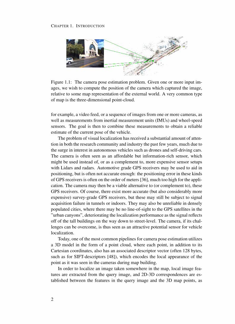
Figure 1.1: The camera pose estimation problem. Given one or more input im-ages, we wish to compute the position of the camera which captured the image,relative to some map representation of the external world. A very common typeof map is the three-dimensional point-cloud.
for example, a video feed, or a sequence of images from one or more cameras, aswell as measurements from inertial measurement units (IMUs) and wheel-speedsensors. The goal is then to combine these measurements to obtain a reliableestimate of the current pose of the vehicle.
The problem of visual localization has received a substantial amount of atten-tion in both the research community and industry the past few years, much due tothe surge in interest in autonomous vehicles such as drones and self-driving cars.The camera is often seen as an affordable but information-rich sensor, whichmight be used instead of, or as a complement to, more expensive sensor setupswith Lidars and radars. Automotive grade GPS receivers may be used to aid inpositioning, but is often not accurate enough: the positioning error in these kindsof GPS receivers is often on the order of meters [36], much too high for the appli-cation. The camera may then be a viable alternative to (or complement to), theseGPS receivers. Of course, there exist more accurate (but also considerably moreexpensive) survey-grade GPS receivers, but these may still be subject to signalacquisition failure in tunnels or indoors. They may also be unreliable in denselypopulated cities, where there may be no line-of-sight to the GPS satellites in the”urban canyons”, deteriorating the localization performance as the signal reflectsoff of the tall buildings on the way down to street-level. The camera, if its chal-lenges can be overcome, is thus seen as an attractive potential sensor for vehiclelocalization.
Today, one of the most common pipelines for camera pose estimation utilizesa 3D model in the form of a point cloud, where each point, in addition to itsCartesian coordinates, also has an associated descriptor vector (often 128 bytes,such as for SIFT-descriptors [48]), which encodes the local appearance of thepoint as it was seen in the cameras during map building.
In order to localize an image taken somewhere in the map, local image fea-tures are extracted from the query image, and 2D-3D correspondences are es-tablished between the features in the query image and the 3D map points, as
2

Figure 1.2: Before pose estimation, matches between the query image and the3D model are established. Note that some of the matches will typically be incor-rect (shown in red). These 2D-3D correspondences are then fed to a camera poseestimation method which computes the pose of the camera for which as many ofthe 3D matches in the map as possible are projected down onto the corresponding2D points in the image.
illustrated in Fig. 1.2. This is typically done by, for each keypoint in the image,finding its approximate nearest neighbour in the map in terms of descriptor dis-tance using a kd-tree search [54]. Using these matches, the pose which agreeswith the largest number of these matches is then estimated. This may be doneusing a perspective-three-point solver [37, 39], in combination with a robust es-timation technique such as RANSAC [26].
This purely geometrical approach based on local image appearance typi-cally works well when the query image is taken under similar conditions as themap. However, if the appearance variation is too large, for instance due to largechanges in viewpoint, lighting, or even seasonal changes, then the local imageappearance may not be discriminative enough to correctly match the 2D fea-tures to the 3D map. This may then yield too few correct matches to accuratelyestimate the camera pose.
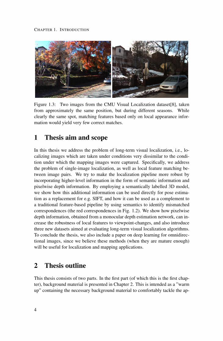
Fig. 1.3 illustrates how the same scene can change in appearance across sea-sons. If an autonomous vehicle is to employ camera-based navigation over along period of time, then it should ideally be able to handle these kinds of visualchanges. Creation of accurate maps is a time-consuming and expensive process,and creating maps for every single conceivable visual condition is unfeasible.Rather, we desire our localization systems to be robust to these kinds of changes.
While the last few years have seen great progress in this area, the visuallocalization systems of today are not able to fully handle these sorts of visualchanges, and developing robust localization methods is a field of active research.It is also the topic of this thesis.
3
CHAPTER 1. INTRODUCTION
Figure 1.3: Two images from the CMU Visual Localization dataset[8], takenfrom approximately the same position, but during different seasons. Whileclearly the same spot, matching features based only on local appearance infor-mation would yield very few correct matches.
1 Thesis aim and scope
In this thesis we address the problem of long-term visual localization, i.e., lo-calizing images which are taken under conditions very dissimilar to the condi-tion under which the mapping images were captured. Specifically, we addressthe problem of single-image localization, as well as local feature matching be-tween image pairs. We try to make the localization pipeline more robust byincorporating higher-level information in the form of semantic information andpixelwise depth information. By employing a semantically labelled 3D model,we show how this additional information can be used directly for pose estima-tion as a replacement for e.g. SIFT, and how it can be used as a complement toa traditional feature-based pipeline by using semantics to identify mismatchedcorrespondences (the red correspondences in Fig. 1.2). We show how pixelwisedepth information, obtained from a monocular depth estimation network, can in-crease the robustness of local features to viewpoint-changes, and also introducethree new datasets aimed at evaluating long-term visual localization algorithms.To conclude the thesis, we also include a paper on deep learning for omnidirec-tional images, since we believe these methods (when they are mature enough)will be useful for localization and mapping applications.
2 Thesis outline
This thesis consists of two parts. In the first part (of which this is the first chap-ter), background material is presented in Chapter 2. This is intended as a ”warmup” containing the necessary background material to comfortably tackle the ap-
4

2. THESIS OUTLINE
pended papers in the second part of the thesis. Readers already familiar with thecamera-pose-estimation problem can likely skip this chapter without any loss ofcomprehension when reading the remainder of the thesis. Chapter 3 summarizesthe contents of the five papers, and clarifies the author’s contribution to each ofthem. Lastly, Chapter 4 concludes the first part of the thesis and presents a finaloutlook on possible future directions for research.
The second part consists of five appended papers, and represents the maincontent and novel research work of the thesis.
5

6

Chapter 2
Background
The main part of this thesis consists of the papers appended in Part II. However,research articles are often quite terse and do not elaborate significantly on thebackground material since the reader is assumed to already be more or less fa-miliar with it. This can make reading papers in a new area very challenging, sincethe overall setting in which the paper takes place may not be fully explained.
The purpose of this chapter is to serve as such a warm-up and summarize therelevant background material necessary to understand the contents of the papersincluded in Part II, and elaborate some more on the general context that may belacking in the individual papers themselves. The structure of the chapter is asfollows: Sec. 1 gives an coarse taxonomy of the visual localization problem, andsome common approaches that may be used to solve it. Sec. 2 introduces whatlocal image features are, how they can be used to establish matches betweenimages, and how they often break down in the long-term localization scenario.Sec. 3 discusses the geometry of camera projection, and how correspondencesbetween 2D image points and 3D map points may be used to calculate camerapose relative to a map. Sec. 4 explains how image-retrieval based visual local-ization works. Lastly, Sec. 5 brings up the topic of semantic segmentations, andsuggests how they may potentially aid in visual localization tasks.
1 Visual localization
As mentioned in the introduction, the problem of visual localization is to deter-mine the position of the camera which captured one or more images with respectto a map. There exist many different variations of this problem, with accompany-ing solutions, depending on what input data is available to aid in the localization(such as the number of images, any prior information on location, data from ad-ditional sensors such as from an inertial measurement unit, Lidar, etc) as well aswhat representation is used for the map.
7
CHAPTER 2. BACKGROUND
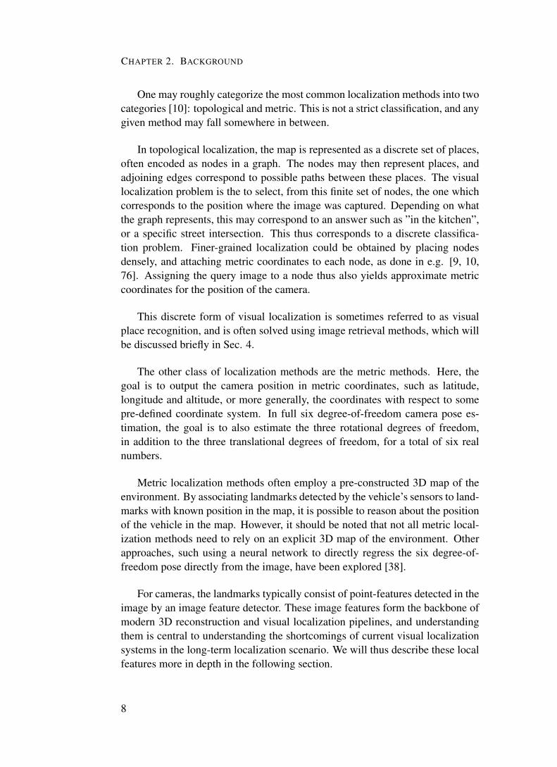
One may roughly categorize the most common localization methods into twocategories [10]: topological and metric. This is not a strict classification, and anygiven method may fall somewhere in between.
In topological localization, the map is represented as a discrete set of places,often encoded as nodes in a graph. The nodes may then represent places, andadjoining edges correspond to possible paths between these places. The visuallocalization problem is the to select, from this finite set of nodes, the one whichcorresponds to the position where the image was captured. Depending on whatthe graph represents, this may correspond to an answer such as ”in the kitchen”,or a specific street intersection. This thus corresponds to a discrete classifica-tion problem. Finer-grained localization could be obtained by placing nodesdensely, and attaching metric coordinates to each node, as done in e.g. [9, 10,76]. Assigning the query image to a node thus also yields approximate metriccoordinates for the position of the camera.
This discrete form of visual localization is sometimes referred to as visualplace recognition, and is often solved using image retrieval methods, which willbe discussed briefly in Sec. 4.
The other class of localization methods are the metric methods. Here, thegoal is to output the camera position in metric coordinates, such as latitude,longitude and altitude, or more generally, the coordinates with respect to somepre-defined coordinate system. In full six degree-of-freedom camera pose es-timation, the goal is to also estimate the three rotational degrees of freedom,in addition to the three translational degrees of freedom, for a total of six realnumbers.
Metric localization methods often employ a pre-constructed 3D map of theenvironment. By associating landmarks detected by the vehicle’s sensors to land-marks with known position in the map, it is possible to reason about the positionof the vehicle in the map. However, it should be noted that not all metric local-ization methods need to rely on an explicit 3D map of the environment. Otherapproaches, such using a neural network to directly regress the six degree-of-freedom pose directly from the image, have been explored [38].
For cameras, the landmarks typically consist of point-features detected in theimage by an image feature detector. These image features form the backbone ofmodern 3D reconstruction and visual localization pipelines, and understandingthem is central to understanding the shortcomings of current visual localizationsystems in the long-term localization scenario. We will thus describe these localfeatures more in depth in the following section.
8

2. LOCAL IMAGE FEATURES
2 Local image features
Image feature (or keypoint) detection and description is one of the most funda-mental problems in computer vision, and forms the foundation on which a largebody of other methods rest [71]. The purpose of the feature detector is to extractfrom an image a set of interest points we believe we will be able to redetect in adifferent image of the same scene, and the purpose of the descriptor is to encodethe appearance of the keypoints into a descriptor vector, such that keypoints inthe first image can be associated to keypoints in the second image (or map).
If the same set of points can be detected in a different image, we can es-tablish point-correspondences between images, or between an image and a 3Dmodel. Image-to-image correspondences can be used for calculating relativecamera pose, which enables subsequent 3D reconstruction of the scene [32].Image-to-model correspondences allow us to compute the camera pose relativeto the model.
In this section we will first briefly discuss keypoint detectors and descriptors,and then have a look at them in the context of long-term visual localization.
2.1 Feature detectors
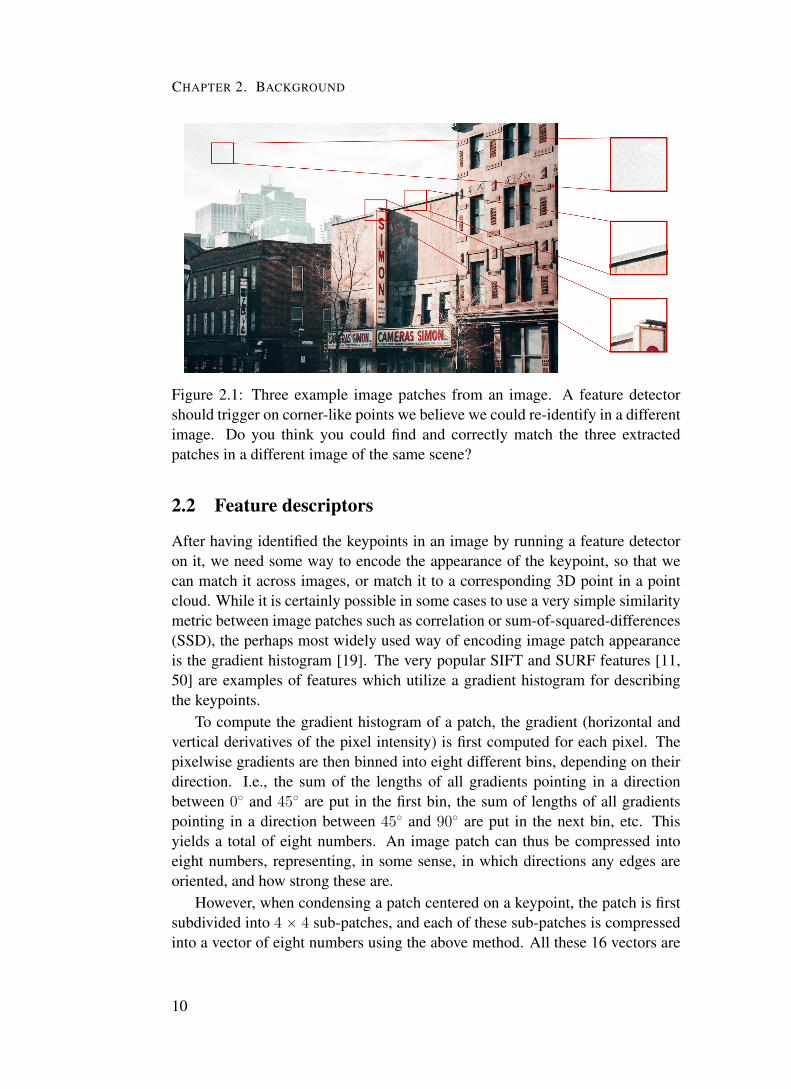
Feature detectors have been studied since the early days of computer vision,and as such there exist a large number of feature detectors (see e.g. [75] for asurvey). Common among most of them is that they try to find corner- or blob-like features in the images; flat areas with uniform brightness are not distinctiveenough to match unambiguously across images, and the same is true for edges,see Fig. 2.1.
Corner detectors work by computing some statistics of the extracted imagepatch. For example, they might examine the Hessian, the Laplacian-of-Gaussian[45], or the Difference-of-Gaussian (DoG) [49] of the image. Other detectorsexamine the auto-correlation function of the image [30, 74]: imagine extracting arectangular patch centered around the point. If the contents of the patch changesconsiderably as we slide the window in any direction (with differences measuredin, perhaps, sum-of-squared difference in pixel intensity between the originalpatch and the translated one), then the point corresponds to a corner. On theother hand, if the patch contents only change in one direction, but are more orless constant in the other direction, the point likely lies on an edge, and it seemsunlikely we would be able to accurately re-identify it in a different image of thesame scene.
9
CHAPTER 2. BACKGROUND
Figure 2.1: Three example image patches from an image. A feature detectorshould trigger on corner-like points we believe we could re-identify in a differentimage. Do you think you could find and correctly match the three extractedpatches in a different image of the same scene?
2.2 Feature descriptors
After having identified the keypoints in an image by running a feature detectoron it, we need some way to encode the appearance of the keypoint, so that wecan match it across images, or match it to a corresponding 3D point in a pointcloud. While it is certainly possible in some cases to use a very simple similaritymetric between image patches such as correlation or sum-of-squared-differences(SSD), the perhaps most widely used way of encoding image patch appearanceis the gradient histogram [19]. The very popular SIFT and SURF features [11,50] are examples of features which utilize a gradient histogram for describingthe keypoints.
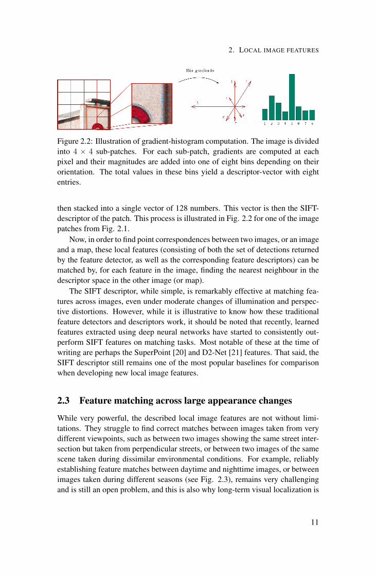
To compute the gradient histogram of a patch, the gradient (horizontal andvertical derivatives of the pixel intensity) is first computed for each pixel. Thepixelwise gradients are then binned into eight different bins, depending on theirdirection. I.e., the sum of the lengths of all gradients pointing in a directionbetween 0˝ and 45˝ are put in the first bin, the sum of lengths of all gradientspointing in a direction between 45˝ and 90˝ are put in the next bin, etc. Thisyields a total of eight numbers. An image patch can thus be compressed intoeight numbers, representing, in some sense, in which directions any edges areoriented, and how strong these are.
However, when condensing a patch centered on a keypoint, the patch is firstsubdivided into 4 ˆ 4 sub-patches, and each of these sub-patches is compressedinto a vector of eight numbers using the above method. All these 16 vectors are
10
2. LOCAL IMAGE FEATURES
Figure 2.2: Illustration of gradient-histogram computation. The image is dividedinto 4 ˆ 4 sub-patches. For each sub-patch, gradients are computed at eachpixel and their magnitudes are added into one of eight bins depending on theirorientation. The total values in these bins yield a descriptor-vector with eightentries.
then stacked into a single vector of 128 numbers. This vector is then the SIFT-descriptor of the patch. This process is illustrated in Fig. 2.2 for one of the imagepatches from Fig. 2.1.
Now, in order to find point correspondences between two images, or an imageand a map, these local features (consisting of both the set of detections returnedby the feature detector, as well as the corresponding feature descriptors) can bematched by, for each feature in the image, finding the nearest neighbour in thedescriptor space in the other image (or map).
The SIFT descriptor, while simple, is remarkably effective at matching fea-tures across images, even under moderate changes of illumination and perspec-tive distortions. However, while it is illustrative to know how these traditionalfeature detectors and descriptors work, it should be noted that recently, learnedfeatures extracted using deep neural networks have started to consistently out-perform SIFT features on matching tasks. Most notable of these at the time ofwriting are perhaps the SuperPoint [20] and D2-Net [21] features. That said, theSIFT descriptor still remains one of the most popular baselines for comparisonwhen developing new local image features.
2.3 Feature matching across large appearance changes
While very powerful, the described local image features are not without limi-tations. They struggle to find correct matches between images taken from verydifferent viewpoints, such as between two images showing the same street inter-section but taken from perpendicular streets, or between two images of the samescene taken during dissimilar environmental conditions. For example, reliablyestablishing feature matches between daytime and nighttime images, or betweenimages taken during different seasons (see Fig. 2.3), remains very challengingand is still an open problem, and this is also why long-term visual localization is
11

CHAPTER 2. BACKGROUND
Figure 2.3: An example of SIFT-feature matching between two images takenfrom approximately the same viewpoint, but during different seasons. A Loweratio of 0.9 was used in the matching process. Not all feature matches are shown,but only those consistent with the estimated epipolar geometry.
difficult.Fig. 2.3 shows an example of SIFT-feature matching between two images
taken from approximately the same viewpoint, but far apart in time (during dif-ferent seasons). Keypoints are extracted using the DoG detector, and then eachfeature in the left image is matched using approximate nearest neighbour match-ing (in descriptor space) to the features in the image to the right. A relativecamera geometry which is consistent with as many matches as possible is calcu-lated, and the figure shows the surviving, geometrically verified matches. Noneof them are correct.
The reason for this failure is two-fold: first of all, the detector does not triggeron the same set of points in the two images (i.e., the detector is not repeatableover these appearance variations), and secondly, the descriptor for a given pointchanges too much between the images to be reliably matched. The low-levelpixel intensity in a local neighbourhood around any given patch looks completelydifferent in the two images, even though they correspond to the same point. Inthe article [1], several extensive experiments are performed showing (and quan-tifying) the non-repeatability of the most popular feature detectors for varyingdegrees of viewpoint and lighting changes.
If a map is constructed from images captured during the same conditionas in the left image, and we then revisit the same area at a later time, whenthe environment looks as in the figure to the right, how do we perform robustvisual localization if traditional local-feature matching yields mostly incorrectmatches? This is the core problem which is discussed in the appended papers inthis thesis.
At this stage, we can make one key observation regarding this simple experi-ment. If I asked you to manually provide a set of, say, ten point correspondences
12

3. STRUCTURE-BASED LOCALIZATION
between the two images, would you be able to? Ideally, if they are to be usedfor camera pose estimation, the error when ”clicking out” the correspondencesshould not be more than a few pixels.
Most likely you would. Though the low-level content of the image may havechanged drastically in any given image patch due to changes in lighting, addedsnow, removed leaves and so on, we can (perhaps with some slight effort) matchpoints based on a higher-level, semantic reasoning. We could match the cornersof the building roof, the corners of the street sign, the tips of the poles in thepicket fence, and so on. None of this would be possible by simply comparingthe low-level image content between pairs of patches; we must reason usingconsiderably more high-level information about the image contents to find thecorrect matches.
It is likely by learning these kinds of higher-level features that local featuresbased on machine learning have started outperforming traditional features in therecent literature. Additionally, this thought experiment seems to suggest thatextracting higher-level scene semantics may be useful for the purpose of visuallocalization. This idea is explored in the first two appended papers in this thesis.
3 Structure-based localizationNow that we have understood how to identify local features in images, and howthese can be matched between images, we will now have a look at how thesefeatures can be used for the task of visual localization. We will first have a look atstructure-based methods, i.e., methods which employ a 3D representation of theenvironment (such as a point cloud) to aid in the localization process. In orderto understand how this is used, we must first have a quick look at the imageformation process for cameras, i.e., the mechanism by which the 3D world isprojected down into a two-dimensional image.
3.1 The camera model
The standard pinhole camera model is a subject which has been written exten-sively about before, and every course on optics, computer vision and computergraphics covers this, so it seems somewhat redundant to write yet another intro-duction. We will here only write down the very basics of camera projection. Formore information, see e.g. Chapter 6 in [31].
The simplest and perhaps most popular camera model is the pinhole cameramodel. A pinhole camera, or a camera obscura, is simply a box with a tiny hole(a pinhole) in one of its sides. When light is emitted from, or scatters off of, anobject in the scene, some of that light might pass through the hole, which we willcall the center of projection O, and will fall onto a point on the opposite side of
13
CHAPTER 2. BACKGROUND
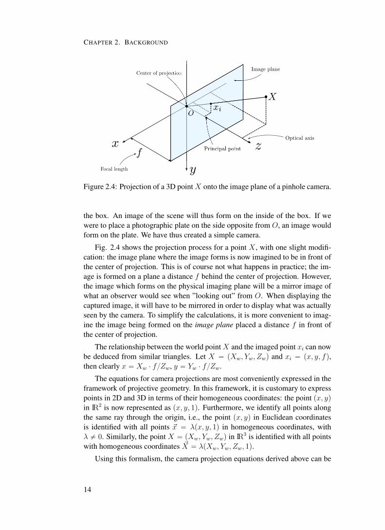
Figure 2.4: Projection of a 3D pointX onto the image plane of a pinhole camera.
the box. An image of the scene will thus form on the inside of the box. If wewere to place a photographic plate on the side opposite from O, an image wouldform on the plate. We have thus created a simple camera.
Fig. 2.4 shows the projection process for a point X , with one slight modifi-cation: the image plane where the image forms is now imagined to be in front ofthe center of projection. This is of course not what happens in practice; the im-age is formed on a plane a distance f behind the center of projection. However,the image which forms on the physical imaging plane will be a mirror image ofwhat an observer would see when ”looking out” from O. When displaying thecaptured image, it will have to be mirrored in order to display what was actuallyseen by the camera. To simplify the calculations, it is more convenient to imag-ine the image being formed on the image plane placed a distance f in front ofthe center of projection.
The relationship between the world pointX and the imaged point xi can nowbe deduced from similar triangles. Let X “ pXw, Yw, Zwq and xi “ px, y, fq,then clearly x “ Xw ¨ f{Zw, y “ Yw ¨ f{Zw.
The equations for camera projections are most conveniently expressed in theframework of projective geometry. In this framework, it is customary to expresspoints in 2D and 3D in terms of their homogeneous coordinates: the point px, yqin IR2 is now represented as px, y, 1q. Furthermore, we identify all points alongthe same ray through the origin, i.e., the point px, yq in Euclidean coordinatesis identified with all points ~x “ λpx, y, 1q in homogeneous coordinates, withλ ‰ 0. Similarly, the point X “ pXw, Yw, Zwq in IR3 is identified with all pointswith homogeneous coordinates ~X “ λpXw, Yw, Zw, 1q.
Using this formalism, the camera projection equations derived above can be
14
3. STRUCTURE-BASED LOCALIZATION
written as
λ~x “
»
–
f 0 00 f 00 0 1
fi
fl
“
I3ˆ3| ~0‰
~X, (2.1)
where ~x and ~X are the homogeneous representations of the points x and X , f isthe focal length, I3ˆ3 is the 3ˆ 3 identity matrix, and ~0 is the vector of all zeroesin IR3.
To obtain the final projection equations for the pinhole camera, two addi-tional things need to be modified. First, the vector x is measured in meters (orwhichever unit of length is used to express the focal length f ). These coordinatesare often called the normalized image coordinates. However, when working withimages, one initially obtains the image features in terms of their pixel coordi-nates in the image, counting rows from up to down, and columns left to right,with the pixel p1, 1q being in the top left corner. To transition from normalizedcoordinates to pixel coordinates, one multiplies the normalized coordinates bythe camera calibration matrix K given by
K “
»
–
αx s cx0 αy cy0 0 1
fi
fl , (2.2)
where αx and αy is the focal length in terms of pixels (these are identical if thepixels are square), s is called the skew and is zero for rectangular pixels, and thepoint pcx, cyq is the principal point in pixel coordinates, i.e., the point where theoptical axis intersects the image plane.
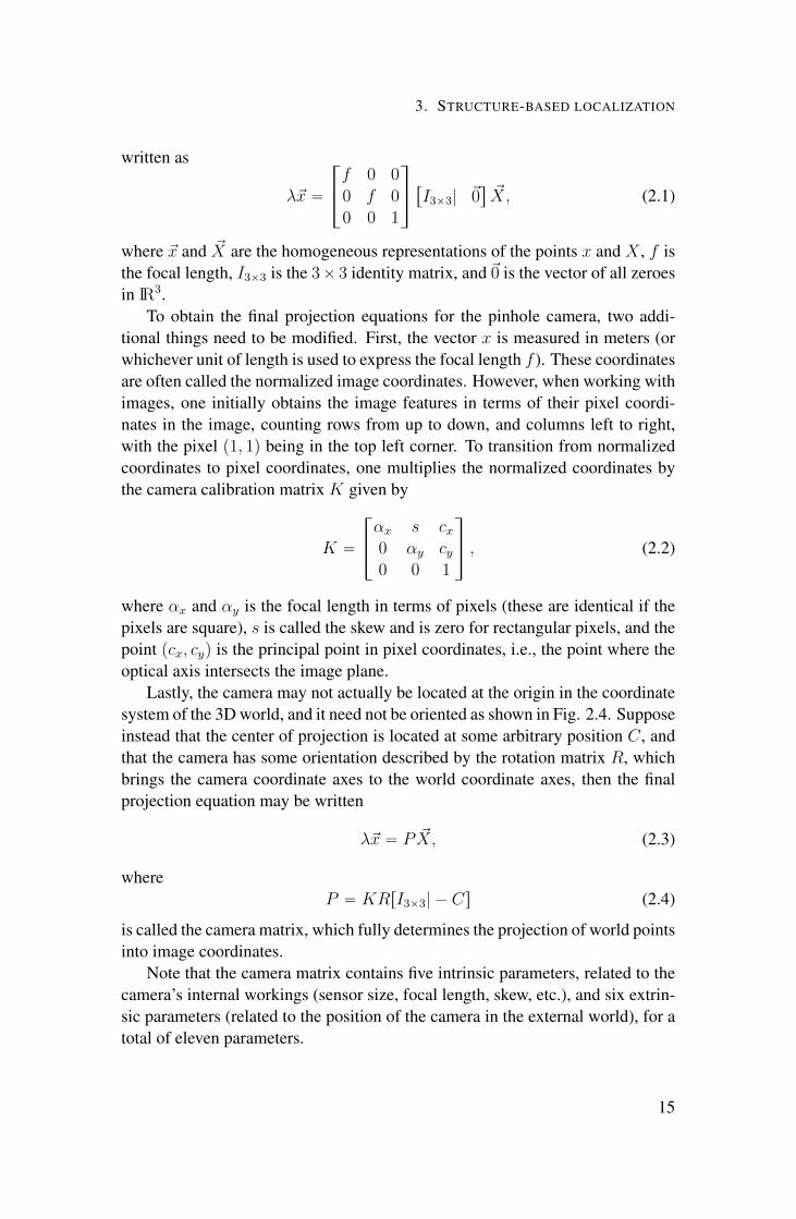
Lastly, the camera may not actually be located at the origin in the coordinatesystem of the 3D world, and it need not be oriented as shown in Fig. 2.4. Supposeinstead that the center of projection is located at some arbitrary position C, andthat the camera has some orientation described by the rotation matrix R, whichbrings the camera coordinate axes to the world coordinate axes, then the finalprojection equation may be written
λ~x “ P ~X, (2.3)
whereP “ KRrI3ˆ3| ´ Cs (2.4)
is called the camera matrix, which fully determines the projection of world pointsinto image coordinates.
Note that the camera matrix contains five intrinsic parameters, related to thecamera’s internal workings (sensor size, focal length, skew, etc.), and six extrin-sic parameters (related to the position of the camera in the external world), for atotal of eleven parameters.
15
CHAPTER 2. BACKGROUND
In the visual localization problems discussed in the papers in this thesis, theinternal parameters have all been determined beforehand in a calibration proce-dure. This is typically done by taking several pictures of a calibration objectwhose physical dimensions are known very precisely [79].
One final thing worth bringing up before moving on to structure-based cam-era pose estimation, is that the pinhole camera model is an idealized, mathemati-cal model for the image formation process. In practice, since the pinhole cameraonly lets in a very small amount of light, a larger aperture is needed (the exposuretime for the world’s first pinhole camera was around eight hours [33]). However,increasing the aperture size leads to blurry images in a pinhole camera, so a lensis placed in the aperture to focus the light. Real optical systems can be quitesophisticated, and the lenses introduce several different kinds of aberrations inthe optical system, one of which is that of non-linear distortion.
An ideal pinhole camera maps lines in 3D to lines in the image, but non-linear distortion causes these lines to map onto curved arcs in the image, oftenwith increasing distortion as one moves away from the principal point. However,this type of distortion has been studied for a long time, with its roots in thephotogrammetric community [13, 25], and simple and accurate models for thenon-linear distortion have been created. These distortion parameters are typicallyestimated during the camera calibration procedure [79], and distorted imagescan then be rectified into corresponding pinhole camera images with sub-pixelaccuracy.
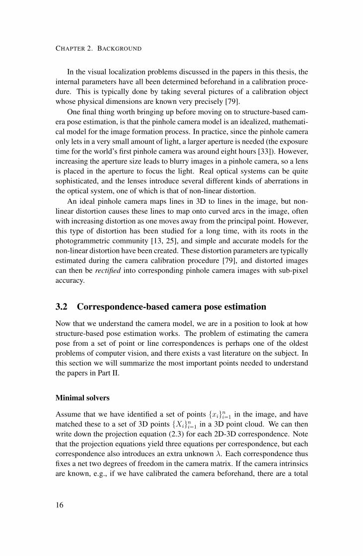
3.2 Correspondence-based camera pose estimation
Now that we understand the camera model, we are in a position to look at howstructure-based pose estimation works. The problem of estimating the camerapose from a set of point or line correspondences is perhaps one of the oldestproblems of computer vision, and there exists a vast literature on the subject. Inthis section we will summarize the most important points needed to understandthe papers in Part II.
Minimal solvers
Assume that we have identified a set of points txiuni“1 in the image, and havematched these to a set of 3D points tXiu
ni“1 in a 3D point cloud. We can then
write down the projection equation (2.3) for each 2D-3D correspondence. Notethat the projection equations yield three equations per correspondence, but eachcorrespondence also introduces an extra unknown λ. Each correspondence thusfixes a net two degrees of freedom in the camera matrix. If the camera intrinsicsare known, e.g., if we have calibrated the camera beforehand, there are a total
16

3. STRUCTURE-BASED LOCALIZATION
of six unknown degrees-of-freedom in the camera matrix, corresponding to theposition of the camera center, and the camera orientation.
It thus seems a total of three correspondences should in general suffice tocompute the camera pose. This is indeed the case. This problem is known as theperspective-three-point problem (P3P), and many different methods for solvingthis problem have been presented over the years [27, 37, 39], with the first knownsolution dating back to 1841 [28].
A classical way of solving the problem is to, for each pair of points, use thelaw of cosines to formulate a quadratic equation in the unknown depths of the 3Dpoints [26, 46, 53]. The three possible pairs thus yield three quadratic equationsin the three unknown depths. One may solve this system in a variety of ways.One way is to use the Sylvester resultant to successively reduce the system intoa single fourth degree equation, which will yield up to four possible solutions tothe problem [27]. In general, a fourth correspondence is needed to disambiguatethe solution. For four or more point correspondences, there exist linear methodsfor calibrated camera pose estimation [2, 58].
In computer vision, methods which solve a problem using only the mini-mum number of correspondences required theoretically are often called minimalsolvers. They play a central role in robust estimation, which we will see below.
The P3P solvers mentioned above is one kind of minimal solver, but thereexist other kinds of minimal solvers for camera pose depending on what kind ofinformation is available. For example, if the gravity direction is known in thecamera reference frame (perhaps supplied by an IMU, or estimated from van-ishing lines in the image [12]), the camera pose only has four extrinsic degreesof freedom left, enabling pose estimation from only two point correspondences[41].
Robust estimation
Once correspondences between the image and a map have been established, feed-ing all correspondences to an n-point pose solver to estimate the camera pose is avery bad idea. The reason is the presence of outliers, in the data, i.e., mismatchedcorrespondences which are completely wrong. Including these in a pose estima-tion routine which minimizes an algebraic error or the geometric reprojectionerror of the correspondences will introduce gross errors in the estimated pose. Away to remove outliers, or to downweigh their contribution to the error functionmust be devised.
The undoubtedly most popular technique for outlier detection and removalin computer vision is the random sample consensus maximization (RANSAC)procedure [26]. This method is not limited to only camera pose estimation, butworks in a wide variety of robust estimation problems, such as line and planefitting, 2D and 3D homography estimation, and so on.
17
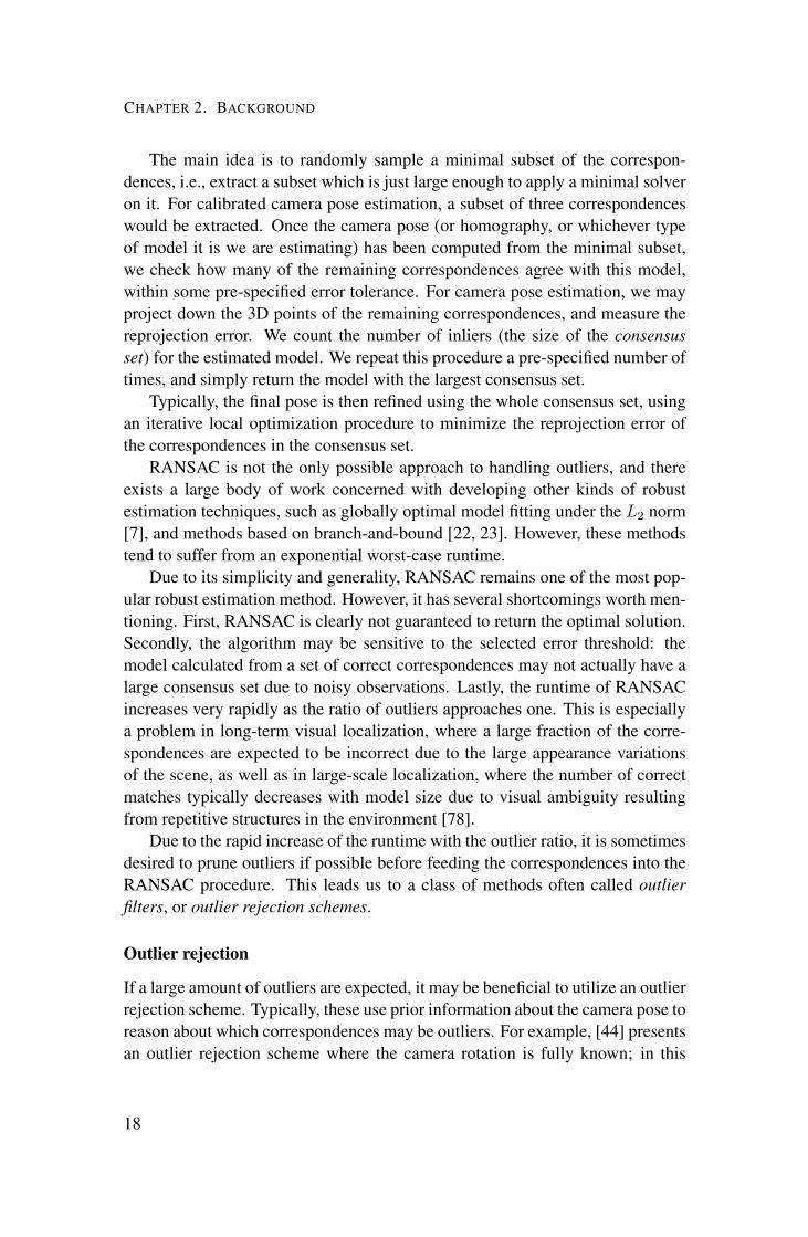
CHAPTER 2. BACKGROUND
The main idea is to randomly sample a minimal subset of the correspon-dences, i.e., extract a subset which is just large enough to apply a minimal solveron it. For calibrated camera pose estimation, a subset of three correspondenceswould be extracted. Once the camera pose (or homography, or whichever typeof model it is we are estimating) has been computed from the minimal subset,we check how many of the remaining correspondences agree with this model,within some pre-specified error tolerance. For camera pose estimation, we mayproject down the 3D points of the remaining correspondences, and measure thereprojection error. We count the number of inliers (the size of the consensusset) for the estimated model. We repeat this procedure a pre-specified number oftimes, and simply return the model with the largest consensus set.
Typically, the final pose is then refined using the whole consensus set, usingan iterative local optimization procedure to minimize the reprojection error ofthe correspondences in the consensus set.
RANSAC is not the only possible approach to handling outliers, and thereexists a large body of work concerned with developing other kinds of robustestimation techniques, such as globally optimal model fitting under the L2 norm[7], and methods based on branch-and-bound [22, 23]. However, these methodstend to suffer from an exponential worst-case runtime.
Due to its simplicity and generality, RANSAC remains one of the most pop-ular robust estimation method. However, it has several shortcomings worth men-tioning. First, RANSAC is clearly not guaranteed to return the optimal solution.Secondly, the algorithm may be sensitive to the selected error threshold: themodel calculated from a set of correct correspondences may not actually have alarge consensus set due to noisy observations. Lastly, the runtime of RANSACincreases very rapidly as the ratio of outliers approaches one. This is especiallya problem in long-term visual localization, where a large fraction of the corre-spondences are expected to be incorrect due to the large appearance variationsof the scene, as well as in large-scale localization, where the number of correctmatches typically decreases with model size due to visual ambiguity resultingfrom repetitive structures in the environment [78].
Due to the rapid increase of the runtime with the outlier ratio, it is sometimesdesired to prune outliers if possible before feeding the correspondences into theRANSAC procedure. This leads us to a class of methods often called outlierfilters, or outlier rejection schemes.
Outlier rejection
If a large amount of outliers are expected, it may be beneficial to utilize an outlierrejection scheme. Typically, these use prior information about the camera pose toreason about which correspondences may be outliers. For example, [44] presentsan outlier rejection scheme where the camera rotation is fully known; in this
18

4. IMAGE-RETRIEVAL BASED LOCALIZATION
Figure 2.5: Visual place recognition formulates the localization problem as animage retrieval problem. Given a query image and a set of database images, findthe database image most similar to the query image (according to some metric).
scenario it is possible to, for each correspondence, calculate an upper bound onthe number of inliers possible for a camera pose which also has that particularcorrespondence is an inlier. If this score is low, it can then be discarded. Thearticle [70] presents an outlier rejection scheme which utilizes prior informationabout camera height and vertical direction. One of the included papers in thisthesis presents a soft outlier rejection scheme based on exploiting the semanticsof the observed image.
4 Image-retrieval based localization
In the beginning of the chapter, we discussed that visual localization methodscan be roughly categorized into metric and topological. The metric methods aretypically 3D structure based, i.e., they employ a 3D model of the environmentand use this to calculate the pose of the camera which captured the query image,as discussed in the previous section.
The topological localization methods, also called visual place recognitionmethods, work in a different manner. Here, the localization problem is insteadformulated as an image search problem: given a set of database images and aquery image, find the database image which most closely resembles the queryimage, see Fig. 2.5.
If metric information is included in the map, for example if the images aregeotagged and have associated GPS metadata, then the position of the query
19

CHAPTER 2. BACKGROUND
image could be approximated by the position of the database image [63].One of the advantages of image retrieval based approaches is that image re-
trieval is a well-studied problem in computer vision, and efficient search strate-gies using vocabulary trees [56] and inverted file indices have been developedfor this problem.
A common implementation of image retrieval is to compute a whole-imagedescriptor for all database image. The whole-image descriptor could be basedon a bag-of-visual-words (BoW) approach [15, 34, 35, 73], or use a vector-of-aggregated-descriptors (VLAD) [3, 72]. The basic idea behind these methodsis to extract local features from the image, such as SIFT descriptors. If thedescriptor space has been quantized beforehand, for example by clustering alldescriptors from a different set of training images using a k-nearest-neighbourapproach, each descriptor extracted from the query image can be assigned tothe nearest cluster. The corresponding whole-image descriptor would then bethe histogram over the number of features assigned to the different clusters (vi-sual words). Learning based approaches such as NetVLAD [4], which computea whole-image descriptor using a neural network, also exist and perform verywell.
To localize an image, this whole-image descriptor is computed for all databaseimages, as well as for the query image. The nearest-neighbour (or k-nearestneighbours) of the query image are then extracted from the database. The poseof the query image can then be approximated using the pose of the top-rankeddatabase image.
Computing a global descriptor from extracted local descriptors yields a morecompact representation of the image, but spatial information is lost. To compen-sate for this, spatial verification and re-ranking [57] can improve the results. Thismeans that the top-ranked images after image retrieval are then re-ranked basedon how well it is possible to fit some geometric transformation that maps corre-spondences from the query image to the database images in question. In otherword, this approach tries to take the spatial layout of the features into account toreconsider the ordering of the suggested best matches. For a survey of the visualplace recognition problem, see [51].
Image retrieval methods have a significant advantage over structure-basedmethods: a database of geotagged images is significantly easier to construct,maintain and extend than a metric 3D reconstruction. It was believed that structure-based approaches yielded more accurate pose estimates than image retrievalbased methods, but there is recent evidence that estimating the camera pose us-ing a local 3D model created ”on-the-fly” from the top-ranked database imagescan yield just as accurate, if not more accurate, poses than pure structure-basedmethods [61]. Additionally, using image retrieval as a pre-processing step in astructure-based system almost always increases the localization performance, as
20

5. SEMANTIC SEGMENTATION
Figure 2.6: An image from the CMU Visual Localization dataset and its corre-sponding semantic segmentation.
we will see in Paper IV.
5 Semantic segmentation
When discussing local image features in Sec. 2, we discussed the problem ofnon-invariance of local features. That is, under viewpoint and illumination changes,the feature detector may trigger on a different set of points, and the feature de-scriptor may change to such an extent that feature matching based on descriptordistances fails completely.
The problem is that traditional descriptors only contain low-level intensityinformation in a patch around the feature points. They contain no higher-level,holistic understanding of the scene. Even in a fairly challenging scenario, ahuman would likely be able to provide matches between two images by utilizingthis high-level information.
In the computer vision community, much progress has been made in recentyears on the problem of semantic segmentation. This problem consists of assign-ing, to each pixel in an image, a label from a pre-defined set of classes. Fig. 2.6shows an example of an image together with its semantic segmentation. Theimage comes from the CMU Visual Localization dataset [10] and the segmenta-tion is performed using the network [77] trained on the Cityscapes classes [17,18]. Cityscapes is a dataset and public benchmark for semantic segmentation ofstreet-view images into semantic classes such as road, sidewalk, car, pedestrian,pole, building, sky and so on. These aim towards a high-level understandingof images taken in street scenes, which may be relevant for the task of visualnavigation for autonomous cars.
Today, semantic segmentation is most commonly performed using some vari-ants of convolutional neural networks (CNNs) [14, 47, 60, 80]. Sometimes, a
21

CHAPTER 2. BACKGROUND
conditional random field (CRF) model is added on top of the network output toencourage a structured segmentation [6, 14, 43].
Even though the local image features may not be invariant to illumination,seasons, day-night changes and so on, a good semantic segmentation algorithmshould ideally be robust to these kinds of variations. If semantic informationcan be reliably extracted under these conditions, it may be possible to utilizethis during the localization process. For example, it may be used for identifyingincorrect matches (a feature detected on a street sign should be matched to a 3Dpoint with the corresponding label), as done in e.g. [5] in the context of objectretrieval.
As observed in [5], the idea of integrating semantic information into the clas-sical computer vision pipelines is something of an emerging theme in the com-puter vision literature, since this has been shown to improve the performanceacross several different tasks. For example, in [42], the authors show that for theproblem of dense stereo reconstruction in road scenes, jointly reasoning aboutdepth and semantic classes improves the performance of the reconstruction dra-matically. The article [64] reaches similar conclusions, where they instead jointlyinfer semantic labels and depths for ”stixels”. Similarly, in [29] a voxelizedmulti-view-stereo reconstruction is performed by joint geometric and semanticreasoning. It is found that the geometry helps enforce the semantics across im-ages, and the semantics help the depth reconstruction e.g. in areas (such as theground) for which depth values are sampled more sparsely.
5.1 Semantics for visual localizationLastly, to wrap up this chapter, we arrive at semantics for visual localization. Asmentioned above, integrating semantics into the classical, geometrical pipelineshas been shown to improve performance. The question is then whether this isalso the case for visual localization. There exists evidence this is indeed the case(see for example [55, 66, 68] for examples where higher-level features such aslane-markings and pole-structures are used for localization), and it is also thetopic of the first two articles appended in Part II.
22
Chapter 3
Thesis Contributions
The topic of this thesis is that of long-term visual localization. Current vi-sual localization approaches typically work well when the mapping images aresimilar in appearance and view-point to the images to be localized, but underchange of viewpoint, illumination or seasons, the localization performance typ-ically degrades rapidly. The non-repeatability of the feature detector, and thenon-invariance of the feature descriptor, are the two main culprits.
We have mentioned in the last chapter that the reason behind the failure ofthe traditional local feature approach in this scenario is that they rely only onlow-level pixel-intensity information, and that incorporating a higher-level sceneunderstanding via the semantic segmentation may potentially alleviate some ofthese problems. This is the topic of two of the included papers (Papers I and II).
While working on the first two articles, we noticed the lack of suitable long-term visual localization datasets to evaluate our methods on. There were a varietyof localization datasets available, but they either did not have sufficient variationin weather, seasons or illumination to evaluate the performance of the methodsin the long-term localization scenario, or, if they did include this variation, theydid not come with accurate six degree-of-freedom camera poses.
Motivated by this, we joined forces with a quite large group of researchersand put together three datasets (where we at Chalmers were responsible mainlyfor one) specifically aimed at evaluating six degree-of-freedom long-term visuallocalization. This work resulted in Paper IV, which is the journal version of aconference article published at CVPR 2018. The benchmark we present in thisarticle has turned out to be fairly popular, and we have hosted several workshopsat CVPR and ICCV on this work, where we accept submissions to a long-termvisual localization challenge.
During the summer of 2019, I had the opportunity to do an internship atNiantic’s research lab in London. The work I did there resulted in Paper III, inwhich we tackle the problem of increasing the robustness of local features toviewpoint changes by utilizing pixelwise depth information gained by running
23

CHAPTER 3. THESIS CONTRIBUTIONS
the images through a monocular depth-estimation network.The last paper, Paper V, differs in theme from the other articles. This paper
considers the problem of how to perform convolutions on spherical data, suchas images obtained from an omnidirectional camera. The original idea for thearticle came up when considering an aspect of the visual localization problem.Specifically, a known challenge is to recognize a previously visited area whenit is revisited, but from a different direction. This could be, for instance, a cardriving down the same road twice, but in opposite directions.
When using a regular perspective camera with limited field of view in thisscenario, the scene will look very different in the two different traversals. Eachtraversal will observe different parts of the scene, and the parts that are covisiblein both traversals will tend to suffer from quite severe perspective distortion.
It seemed to me that this problem would be almost completely bypassed ifan omnidirectional camera was employed instead. In this case the two traversalswould observe essentially the same scene, and it should be possible to approxi-mately align the images with only a rotation. Learned local features have recentlystarted outperforming traditional local features for long-term localization, and Iwondered if these learned features could be applied to omnidirectional imagery.
However, it turned out that the question of how to perform convolutions onspherical data has not yet been fully settled, and it felt necessary to perform somemore foundational work in this area to better understand this problem beforeturning our attention to applications. The result of this work is presented inPaper V.
In the remainder of this chapter we present a high-level summary of each ofthe included papers in turn. The full papers are appended in Part II.
Paper IC. Toft, C. Olsson, F. Kahl. ”Long-term 3D Localization and Pose from Seman-tic Labellings”. Presented at the 3D Reconstruction Meets Semantics Workshopat the International Conference on Computer Vision 2017.
This paper was something of a pilot-study where we examined how well itis possible to perform single-image visual localization, using only the semanticsegmentation of the query image. In other words, is the semantic informationalone sufficient for visual localization? The method was evaluated on two smallsubsets of the Oxford RobotCar dataset, each the size of a few city blocks. Themethod uses an image-retrieval method (based only on the semantic segmenta-tion), and then refines the 6 degree-of-freedom (DoF) camera pose by minimiz-ing a cost function based on how well the reprojection of a semantically labelled3D model, consisting of semantically labelled points and curves of the envi-
24
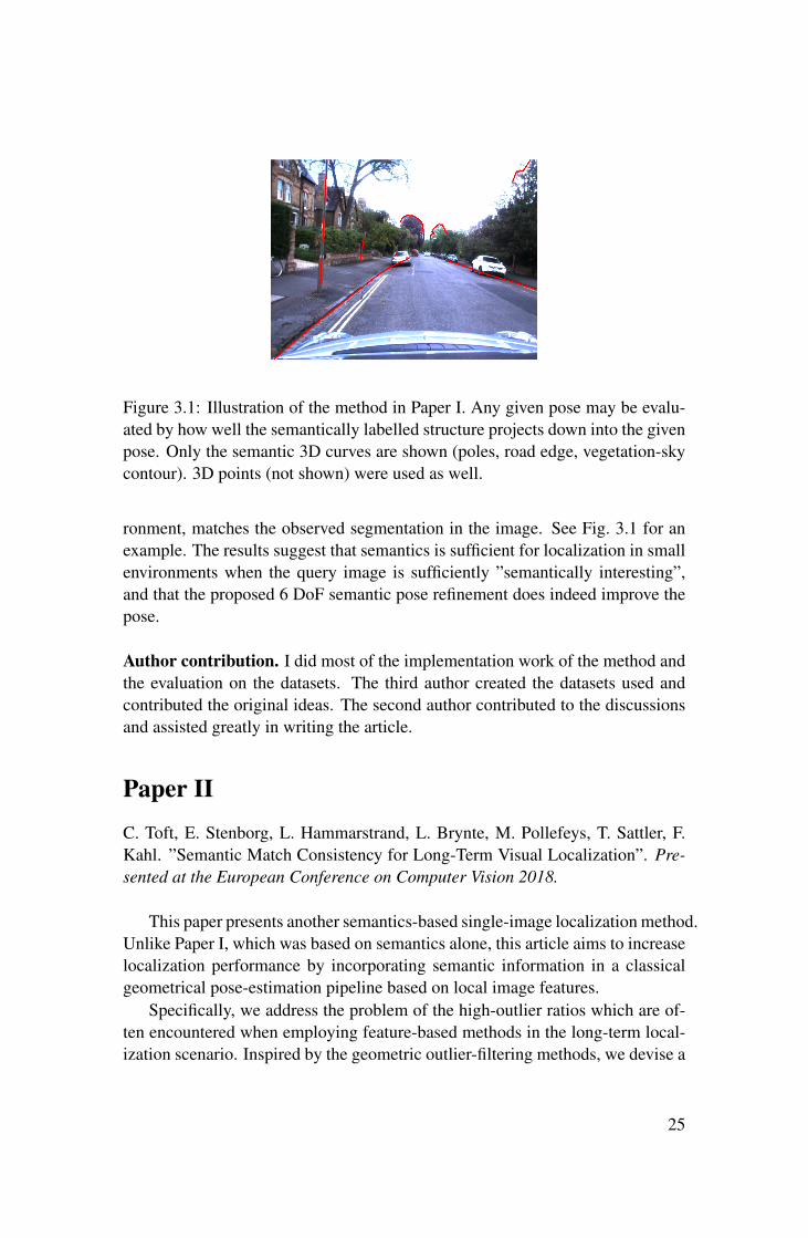
Figure 3.1: Illustration of the method in Paper I. Any given pose may be evalu-ated by how well the semantically labelled structure projects down into the givenpose. Only the semantic 3D curves are shown (poles, road edge, vegetation-skycontour). 3D points (not shown) were used as well.
ronment, matches the observed segmentation in the image. See Fig. 3.1 for anexample. The results suggest that semantics is sufficient for localization in smallenvironments when the query image is sufficiently ”semantically interesting”,and that the proposed 6 DoF semantic pose refinement does indeed improve thepose.
Author contribution. I did most of the implementation work of the method andthe evaluation on the datasets. The third author created the datasets used andcontributed the original ideas. The second author contributed to the discussionsand assisted greatly in writing the article.
Paper II
C. Toft, E. Stenborg, L. Hammarstrand, L. Brynte, M. Pollefeys, T. Sattler, F.Kahl. ”Semantic Match Consistency for Long-Term Visual Localization”. Pre-sented at the European Conference on Computer Vision 2018.
This paper presents another semantics-based single-image localization method.Unlike Paper I, which was based on semantics alone, this article aims to increaselocalization performance by incorporating semantic information in a classicalgeometrical pose-estimation pipeline based on local image features.
Specifically, we address the problem of the high-outlier ratios which are of-ten encountered when employing feature-based methods in the long-term local-ization scenario. Inspired by the geometric outlier-filtering methods, we devise a
25

CHAPTER 3. THESIS CONTRIBUTIONS
3D Scene Model
Query Image Semantic Segmentation
2D-3D Matching
Local FeatureExtraction
WeightedRANSAC-basedPose Estimation
PoseOptimization
Semantic Consistency Scoring
consistent match inconsistent match
Figure 3.2: The general pipeline of the method presented in paper II. The methodis based on a traditional feature-based pipeline, but each feature is scored de-pending on how well it agrees with the overall semantics of the scene and image.This score is then used to weight the sampling probabilities in the RANSACloop.
semantic outlier filter, which, like the geometric outlier filters, uses prior knowl-edge about the camera height above the ground plane as well as the vertical direc-tion, to reason about the likelihood of each correspondence being an inlier. Themethod is evaluated on two self-driving car datasets, and we show that, under theconditions mentioned, the method can significantly increase the performance ofa classical P3P RANSAC based pipeline.
One of the main advantages of the proposed method is that it is fully parallelin the number of correspondences: each correspondence can be scored indepen-dently of the others, and the method of scoring correspondences depends onlyon projections and angle calculations. As such, it would be very suitable for anefficient GPU implementation, though in the paper only a sequential MATLABimplementation was performed.
Author contribution. The last author supplied the original idea, and I imple-mented the method and all evaluation scripts. The other authors helped withdiscussions, writing, figures and provided semantic segmentations for the usedimages.
Paper III
C. Toft, D. Turmukhambetov, T. Sattler, F. Kahl, and G. Brostow. “Single-ImageDepth Prediction Makes Feature Matching Easier”. Presented at the EuropeanConference on Computer Vision 2020.
When matching local features between two images, the performance de-grades with increasing viewpoint difference between the images. In this paper,
26
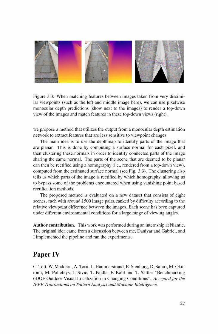
Figure 3.3: When matching features between images taken from very dissimi-lar viewpoints (such as the left and middle image here), we can use pixelwisemonocular depth predictions (show next to the images) to render a top-downview of the images and match features in these top-down views (right).
we propose a method that utilizes the output from a monocular depth estimationnetwork to extract features that are less sensitive to viewpoint changes.
The main idea is to use the depthmap to identify parts of the image thatare planar. This is done by computing a surface normal for each pixel, andthen clustering these normals in order to identify connected parts of the imagesharing the same normal. The parts of the scene that are deemed to be planarcan then be rectified using a homography (i.e., rendered from a top-down view),computed from the estimated surface normal (see Fig. 3.3). The clustering alsotells us which parts of the image is rectified by which homography, allowing usto bypass some of the problems encountered when using vanishing point basedrectification methods.
The proposed method is evaluated on a new dataset that consists of eightscenes, each with around 1500 image pairs, ranked by difficulty according to therelative viewpoint difference between the images. Each scene has been capturedunder different environmental conditions for a large range of viewing angles.
Author contribution. This work was performed during an internship at Niantic.The original idea came from a discussion between me, Daniyar and Gabriel, andI implemented the pipeline and ran the experiments.
Paper IV
C. Toft, W. Maddern, A. Torii, L. Hammarstrand, E. Stenborg, D. Safari, M. Oku-tomi, M. Pollefeys, J. Sivic, T. Pajdla, F. Kahl and T. Sattler ”Benchmarking6DOF Outdoor Visual Localization in Changing Conditions”. Accepted for theIEEE Transactions on Pattern Analysis and Machine Intelligence.
27
CHAPTER 3. THESIS CONTRIBUTIONS
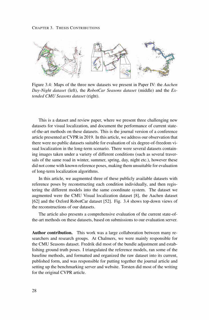
Figure 3.4: Maps of the three new datasets we present in Paper IV: the AachenDay-Night dataset (left), the RobotCar Seasons dataset (middle) and the Ex-tended CMU Seasons dataset (right).
This is a dataset and review paper, where we present three challenging newdatasets for visual localization, and document the performance of current state-of-the-art methods on these datasets. This is the journal version of a conferencearticle presented at CVPR in 2019. In this article, we address our observation thatthere were no public datasets suitable for evaluation of six degree-of-freedom vi-sual localization in the long-term scenario. There were several datasets contain-ing images taken under a variety of different conditions (such as several traver-sals of the same road in winter, summer, spring, day, night etc.), however thesedid not come with known reference poses, making them unsuitable for evaluationof long-term localization algorithms.
In this article, we augmented three of these publicly available datasets withreference poses by reconstructing each condition individually, and then regis-tering the different models into the same coordinate system. The dataset weaugmented were the CMU Visual localization dataset [8], the Aachen dataset[62] and the Oxford RobotCar dataset [52]. Fig. 3.4 shows top-down views ofthe reconstructions of our datasets.
The article also presents a comprehensive evaluation of the current state-of-the-art methods on these datasets, based on submissions to our evaluation server.
Author contribution. This work was a large collaboration between many re-searchers and research groups. At Chalmers, we were mainly responsible forthe CMU Seasons dataset. Fredrik did most of the bundle adjustment and estab-lishing ground truth poses. I triangulated the reference models, ran some of thebaseline methods, and formatted and organized the raw dataset into its current,published form, and was responsible for putting together the journal article andsetting up the benchmarking server and website. Torsten did most of the writingfor the original CVPR article.
28

(a)
φ1 φ2
θ1
θ2
(b)
Figure 3.5: We show that a general linear SO(2) equivariant transform fromL2pS2q Ñ L2pS2q can be interpreted as computing the correlation between theinput signal f and a θ-dependent filter hθ, and how these take the form of block-diagonal matrices in the spherical Fourier domain.
Paper V
C. Toft, G. Bökman, and F. Kahl. ”Azimuthal Rotational Equivariance in Spher-ical CNNs”. Submitted for review to the International Conference on LearningRepresentations 2021.
In this paper we consider the problem of designing neural networks for spher-ical data. Convolutional neural networks have achieved outstanding success inthe analysis of planar data, but it is not immediately clear how to generalize thesenetworks to operate on spherical data.
Two of the defining characteristics of a (planar) convolution are its linear-ity and equivariance to translations. Using these as guiding principles, one candefine convolutions on the sphere equivariant to arbitrary SO(3) rotations, asdone by e.g. Cohen et al., Esteves et al. and Kondor et al. [16, 24, 40]. How-ever, several recently proposed high-performing networks on the sphere applyconvolutional operators that are not fully SO(3) equivariant (for example, theymay include horizontal and vertical derivatives). We note, however, that theseconvolutions are linear and exhibit SO(2) equivariance.
Thus, in this paper we ask how an operator fromL2pS2q Ñ L2pS2qmust lookin order for it to be linear and SO(2) equivariant. We show that these operatorsmust admit a block-diagonal representation in the spherical Fourier domain ifthey operate on band-limited input data. Additionally, we show how these maybe intepreted as a correlation with an azimuthal-dependent filter (see Fig. 3.5).
Lastly, we show how an existing state-of-the-art SO(2) equivariant pipeline
29

CHAPTER 3. THESIS CONTRIBUTIONS
for spherical data can be recreated in our framework, showing increased invari-ance to azimuthal rotations of the test data.
Author contribution. I came up with the idea for the paper, and proved the re-sult in proposition 1 regarding the spectral characterization of SO(2) equivariantlinear operators from L2pS2q Ñ L2pS2q. Additionally, I ran the experiments onthe MNIST dataset, while the second author ran the experiments on the Model-Net40 dataset.
30

Chapter 4
Conclusion and Future Outlook
In this thesis, we have presented work on the problem of robust visual local-ization, mainly by adressing the following points:
• We have examined how to incorporate semantic information to aid in thevisual localization process.
• We have examined a possible way to utilize depth estimates to extract fea-tures less sensitive to viewpoint changes.
• We have developed new datasets, and a public benchmark, to enable accu-rate and fair evaluation of the performance of visual localization methodsin the long-term localization scenario.
• We have worked on untangling some of the theory of spherical convolu-tions, which may eventually lead to learned local features for omnidirec-tional cameras.
The field of visual localization has seen considerable progress since I em-barked on this journey over four years ago. Looking back to my earliest work onincorporating semantic information in localization, it is already somewhat out-dated and has been superseded by new ideas, but I believe that work served as animportant stepping stone that provided valuable insights.
For instance, I believe one of the main takeaways from Papers I and II is thatit is possible to perform visual localization without relying only on the matched3D points; the unmatched points also provide important information regardingthe likelihood of a given hypothesized pose being correct. Additionally, in thefirst paper we saw some indications that it might even be possible to performlocalization without relying on local features at all. This line of thinking waspursued in later work, with some promising results in the sequential localizationscenario, where we saw that good localization results can be obtained in the long-term scenario without relying on traditional feature matching at all. Instead, only
31

CHAPTER 4. CONCLUSION AND FUTURE OUTLOOK
the consistency of the projected semantic model was used. See e.g. subsidiarypublications (d) and (e).
When speaking of localization performance, a question which has recurredcontinually throughout the work has been that of: What localization error is ac-ceptable? How do we know when the localization problem has been solved?What framerate do we need to be able to handle? At the moment, I am not awareof any work which provides general answers to these questions. The localizationperformance of the state-of-the-art algorithms on our benchmark suggest that thelocalization methods are rapidly improving, but there is still room for improve-ment for the very challenging scenarios, such as day-night changes. But it is notquite clear what accuracy is required for e.g. autonomous driving or augmentedreality, or what accuracy is realistic to expect.
In the following section, I expand on some directions for future research Ibelieve are promising regarding the visual localization problem.
1 Future work
1.1 Learned features
One approach which has recently caught on is to learn a feature detector anddescriptor. I.e, to train a neural network to output a detection heatmap and cor-responding dense features, or different variations thereof. In other words, traina detector which tends to trigger on points which are long-term stable and notsensitive to viewpoint differences. This might be corners of windows, rooftopcorners, street signs, and so on (or any other kind of point which the system canreliably re-identify). Popular learned features include SuperPoint [20], D2-Net[21] and R2D2 [59]. One of the problems which may arise when training thisform of feature, is that ground-truth correspondences will be needed, i.e., thesystem needs to know which features actually are stable such that it can learnfrom these. We believe our new datasets may be useful to other researchers inthis regard.
Another related approach which seems promising, and is related in spiritto the semantic localization approaches in Papers I and II, is to perform local-ization by finding the pose which maximizes the consistency between the ob-served dense features extracted from an image using a neural network, and thefeatures of 3D points downprojected onto the image from a hypothesized pose.As in paper I, such a method does not rely on explicit feature matches, and usesall contents of the image and scene to reason about the camera pose.
Such an approach is used e.g. by the GN-Net method [69]. This kind ofmethod is also fairly similar to direct methods for visual odometry, in the sensethat it is essentially correspondence free, but where the alignment error is based
32

1. FUTURE WORK
on feature distance rather than photometric error. This approach would also makeit possible to train a feature extraction network by directly minimizing the local-ization error.
1.2 Incorporate 3D information during feature matchingAnother approach is to incorporate 3D information into the feature extraction ormatching process. This is particularly relevant if a stereo setup is used, or if awell-performing monocular depth estimation network is available. This is verysimilar to the approach used in Paper III, but there is still room for improvementhere. It might be possible to compute the viewpoint invariant descriptor withoutexplicit unwarping of the flat surfaces, or perhaps to encode the surface shape fornon-planar surfaces into the descriptor. If accurate surface normal estimates areavailable, then these may also provide constraints during the feature matchingprocess.
1.3 Improved datasetsWhile we have provided three new datasets that we believe are useful for thecommunity and a step in the right direction, the story is not over here, and thereis still a need for even more comprehensive datasets to properly evaluate local-ization methods in the long-term scenario.
In particular, none of our datasets are particularly suited for evaluating se-quential localization methods. It is not reasonable or realistic to expect single-image methods to work in all scenarios, and in most practical applications, suchas autonomous driving or augmented reality, the pose estimate will be basedon an entire history of data. As such, we believe future reasearch should focusmore towards sequential methods. To evaluate these, large-scale cross-seasonaldatasets captured at high frame-rates with corresponding IMU data would bevaluable. As far as we are aware, no such datasets exist, at least publically.
1.4 Omnidirectional camerasLastly, to wrap up Part I, it seems that omnidirectional cameras would be veryuseful for the task of visual localization, but very few localization methods seemto focus on, or evaluate the performance for, this kind of camera. For instance,re-localizing a car driving down the same road as before, but in the oppositedirection, is very challenging with a regular camera with a limited field of view,but for an omnidirectional camera, this scenario should pose no extra difficulty.
Omnidirectional cameras also seem especially suited for this task due to theirfull field of view: they will not as frequently encouter the situations often en-countered for regular cameras, where there simply is not anything informative
33

CHAPTER 4. CONCLUSION AND FUTURE OUTLOOK
inside the current image. However, how to develop neural networks for learninglocal features for omnidirectional cameras is, as far as we are aware, still an openproblem.
34

Bibliography
[1] Henrik Aanæs, Anders Lindbjerg Dahl, and Kim Steenstrup Pedersen.“Interesting Interest Points”. In: International Journal of Computer Vision97.1 (Mar. 2012), pp. 18–35.
[2] Adnan Ansar and Konstantinos Daniilidis. “Linear pose estimation frompoints or lines”. In: IEEE Transactions on Pattern Analysis and MachineIntelligence 25.5 (2003), pp. 578–589.
[3] Relja Arandjelovic and Andrew Zisserman. “All about VLAD”. In: Pro-ceedings of the IEEE conference on Computer Vision and Pattern Recog-nition. 2013, pp. 1578–1585.
[4] R. Arandjelovic et al. “NetVLAD: CNN architecture for weakly super-vised place recognition”. In: CVPR. 2016.
[5] Relja Arandjelovic and Andrew Zisserman. “Visual Vocabulary with a Se-mantic Twist”. In: ACCV. 2014.
[6] Anurag Arnab et al. “Conditional random fields meet deep neural net-works for semantic segmentation: Combining probabilistic graphical mod-els with deep learning for structured prediction”. In: IEEE Signal Process-ing Magazine 35.1 (2018), pp. 37–52.
[7] Erik Ask, Olof Enqvist, and Fredrik Kahl. “Optimal Geometric FittingUnder the Truncated L2-Norm”. In: Conference Computer Vision and Pat-tern Recognition. 2013.
[8] H. Badino, D. Huber, and T. Kanade. “Visual Topometric Localization”.In: Intelligent Vehicles Symposium (IV). Baden-Baden, Germany, June2011.
[9] H. Badino et al. “Real-Time Topometric Localization”. In: ICRA. 2012.
[10] Hernán Badino, D Huber, and Takeo Kanade. “Visual topometric local-ization”. In: Intelligent Vehicles Symposium (IV), 2011 IEEE. IEEE. 2011,pp. 794–799.
[11] H. Bay et al. “SURF: Speeded Up Robust Features”. In: European Con-ference on Computer Vision 110.3 (2008), pp. 346–359.
35
BIBLIOGRAPHY
[12] J-C. Bazin et al. “Globally Optimal Line Clustering and Vanishing PointEstimation in Manhattan World”. In: Conference Computer Vision andPattern Recognition. 2012.
[13] Duane C. Brown. “Close-range camera calibration”. In: Photogramm. Eng37.8 (1971), pp. 855–866.
[14] Liang-Chieh Chen et al. “Deeplab: Semantic image segmentation withdeep convolutional nets, atrous convolution, and fully connected crfs”.In: IEEE transactions on pattern analysis and machine intelligence 40.4(2018), pp. 834–848.
[15] O. Chum et al. “Total Recall: Automatic Query Expansion with a Genera-tive Feature Model for Object Retrieval”. In: International Conference onComputer Vision. 2007.
[16] Taco S Cohen et al. “Spherical CNNs”. In: 2018.
[17] Marius Cordts et al. “The cityscapes dataset”. In: CVPR Workshop on theFuture of Datasets in Vision. Vol. 1. 2. 2015, p. 3.
[18] Marius Cordts et al. “The Cityscapes Dataset for Semantic Urban SceneUnderstanding”. In: Proc. of the IEEE Conference on Computer Visionand Pattern Recognition (CVPR). 2016.
[19] N. Dalal and B. Triggs. “Histograms of Oriented Gradients for HumanDetection”. In: CVPR. San Diego, USA, 2005, pp. 886–893.
[20] Daniel DeTone, Tomasz Malisiewicz, and Andrew Rabinovich. “Super-point: Self-supervised interest point detection and description”. In: Pro-ceedings of the IEEE Conference on Computer Vision and Pattern Recog-nition Workshops. 2018, pp. 224–236.
[21] Mihai Dusmanu et al. “D2-Net: A Trainable CNN for Joint Descriptionand Detection of Local Features”. In: Proceedings of the IEEE Conferenceon Computer Vision and Pattern Recognition. 2019, pp. 8092–8101.
[22] O. Enqvist and F. Kahl. “Robust Optimal Pose Estimation”. In: EuropeanConference on Computer Vision. 2008.
[23] Olof Enqvist, Klas Josephson, and Fredrik Kahl. “Optimal correspon-dences from pairwise constraints”. In: Computer Vision, 2009 IEEE 12thInternational Conference on. IEEE. 2009, pp. 1295–1302.
[24] Carlos Esteves et al. “Learning SO(3) equivariant representations withspherical CNNs”. In: European Conference on Computer Vision. 2018.
[25] Wolfgang Faig. “Calibration of close-range photogrammetric systems: Math-ematical formulation”. In: Photogrammetric engineering and remote sens-ing 41.12 (1975).
36
BIBLIOGRAPHY
[26] M. Fischler and R. Bolles. “Random Sample Consensus: A Paradigm forModel Fitting with Applications to Image Analysis and Automated Car-tography”. In: Communications of the ACM (1981).
[27] Xiao-Shan Gao et al. “Complete solution classification for the perspective-three-point problem”. In: IEEE transactions on pattern analysis and ma-chine intelligence 25.8 (2003), pp. 930–943.
[28] J. A. Grunert. “Das Pothenot’sche Problem in erweiterter Gestalt; nebstBemerkungen über seine Anwendung in der Geodäsie”. In: Grunert Archivder Mathematik und Physik (1841).
[29] Christian Hane et al. “Joint 3D scene reconstruction and class segmenta-tion”. In: Proceedings of the IEEE Conference on Computer Vision andPattern Recognition. 2013, pp. 97–104.
[30] C. Harris and M. Stephens. “A Combined Corner and Edge Detector”. In:Alvey Vision Conference. 1988.
[31] R. I. Hartley and A. Zisserman. Multiple View Geometry in Computer Vi-sion. Cambridge University Press, 2000.
[32] R. I. Hartley and A. Zisserman. Multiple View Geometry in Computer Vi-sion. Second. Cambridge University Press, ISBN: 0521540518, 2004.
[33] E. Hecht. Optics. Addison-Wesley, Reading, Mass., 1987.
[34] Herve Jegou, Hedi Harzallah, and Cordelia Schmid. “A contextual dis-similarity measure for accurate and efficient image search”. In: ComputerVision and Pattern Recognition, 2007. CVPR’07. IEEE Conference on.IEEE. 2007, pp. 1–8.
[35] H. Jégou, M. Douze, and C. Schmid. “On the burstiness of visual ele-ments”. In: CVPR. 2009.
[36] E. Kaplan and C. Hegarty. Understanding GPS: Principles and Appli-cations, Second Edition. Artech House mobile communications series.Artech House, 2005.
[37] Tong Ke and Stergios I Roumeliotis. “An efficient algebraic solution to theperspective-three-point problem”. In: arXiv preprint arXiv:1701.08237 (2017).
[38] A. Kendall, M. Grimes, and R. Cipolla. “PoseNet: A Convolutional Net-work for Real-Time 6-DOF Camera Relocalization”. In: International Con-ference on Computer Vision. 2015.
[39] L Kneip, D Scaramuzza, and R Siegwart. “A Novel Parametrization of thePerspective-Three-Point Problem for a Direct Computation of AbsoluteCamera Position and Orientation”. In: CVPR. 2011.
37

BIBLIOGRAPHY
[40] Risi Kondor, Zhen Lin, and Shubhendu Trivedi. “Clebsch–Gordan nets: Afully fourier space spherical convolutional neural network”. In: Advancesin Neural Information Processing Systems. 2018.
[41] Zuzana Kukelova, Martin Bujnak, and Tomas Pajdla. “Closed-form solu-tions to minimal absolute pose problems with known vertical direction”.In: Asian Conference Computer Vision. 2010.
[42] Lubor Ladický et al. “Joint optimization for object class segmentation anddense stereo reconstruction”. In: International Journal of Computer Vision100.2 (2012), pp. 122–133.
[43] Måns Larsson. “End-to-end Learning of Deep Structured Models for Se-mantic Segmentation”. PhD thesis. Department of Signals and Systems,Chalmers University of Technology, 2018.
[44] V. Larsson et al. “Outlier rejection for absolute pose estimation with knownorientation”. In: British Machine Vision Conference. 2016.
[45] Tony Lindeberg. “Feature detection with automatic scale selection”. In:International journal of computer vision 30.2 (1998), pp. 79–116.
[46] Seppo Linnainmaa, David Harwood, and Larry S Davis. “Pose determina-tion of a three-dimensional object using triangle pairs”. In: IEEE Transac-tions on Pattern Analysis and Machine Intelligence 10.5 (1988), pp. 634–647.
[47] Jonathan Long, Evan Shelhamer, and Trevor Darrell. “Fully convolutionalnetworks for semantic segmentation”. In: Proceedings of the IEEE confer-ence on computer vision and pattern recognition. 2015, pp. 3431–3440.
[48] D. Lowe. “Distinctive image features from scale-invariant keypoints”. In:International Journal of Computer Vision 60.2 (2004), pp. 91–110.
[49] David G Lowe. “Distinctive image features from scale-invariant keypoints”.In: International journal of computer vision 60.2 (2004), pp. 91–110.
[50] David G. Lowe. “Distinctive Image Features from Scale-Invariant Key-points”. In: International Journal of Computer Vision 60.2 (2004), pp. 91–110.
[51] Stephanie Lowry et al. “Visual place recognition: A survey”. In: IEEETransactions on Robotics 32.1 (2016), pp. 1–19.
[52] Will Maddern et al. “1 Year, 1000km: The Oxford RobotCar Dataset”.In: The International Journal of Robotics Research 36.1 (2017), pp. 3–15.eprint: http://ijr.sagepub.com/content/early/2016/11/28/0278364916679498.full.pdf+html.
[53] EL Merritt. “Explicit three-point resection in space”. In: PhotogrammetricEngineering 15.4 (1949), pp. 649–655.
38

BIBLIOGRAPHY
[54] Marius Muja and David G. Lowe. “Fast Approximate Nearest Neighborswith Automatic Algorithm Configuration”. In: Int. Conf. on Computer Vi-sion Theory and Applications. 2009.
[55] T. Naseer et al. “Semantics-aware Visual Localization under ChallengingPerceptual Conditions”. In: ICRA. 2017.
[56] D. Nistér and H. Stewénius. “Scalable Recognition with a VocabularyTree”. In: CVPR. Vol. II. New York City, USA, 2006, pp. 2161–2168.
[57] J. Philbin et al. “Object Retrieval with Large Vocabularies and Fast Spa-tial Matching”. In: Conference Computer Vision and Pattern Recognition.2007.
[58] L. Quan and Z. Lan. “Linear N ď 4-Point Camera Pose Determination”.In: PAMI 21.8 (Aug. 1999), pp. 774–780.
[59] Jerome Revaud et al. “R2D2: Reliable and Repeatable Detector and De-scriptor”. In: Advances in Neural Information Processing Systems. 2019,pp. 12405–12415.
[60] Olaf Ronneberger, Philipp Fischer, and Thomas Brox. “U-net: Convo-lutional networks for biomedical image segmentation”. In: InternationalConference on Medical image computing and computer-assisted interven-tion. Springer. 2015, pp. 234–241.
[61] Torsten Sattler et al. “Are Large-Scale 3D Models Really Necessary forAccurate Visual Localization?” In: CVPR. 2017.
[62] Torsten Sattler et al. “Image Retrieval for Image-Based Localization Re-visited”. In: British Machine Vision Conference. 2012.
[63] G. Schindler, M. Brown, and R. Szeliski. “City-Scale Location Recogni-tion”. In: CVPR. 2007.
[64] Lukas Schneider et al. “Semantic stixels: Depth is not enough”. In: Intel-ligent Vehicles Symposium (IV), 2016 IEEE. IEEE. 2016, pp. 110–117.
[65] Johannes L. Schönberger and Jan-Michael Frahm. “Structure-From-MotionRevisited”. In: CVPR. 2016.
[66] Markus Schreiber, Carsten Knöppel, and Uwe Franke. “LaneLoc: Lanemarking based localization using highly accurate maps”. In: IV. 2013.
[67] N. Snavely, S.M Seitz, and R. Szeliski. “Photo tourism: Exploring photocollections in 3D”. In: ACM SIGGRAPH (2006).
[68] Robert Spangenberg, Daniel Goehring, and Raúl Rojas. “Pole-based local-ization for autonomous vehicles in urban scenarios”. In: Intelligent Robotsand Systems (IROS), 2016 IEEE/RSJ International Conference on. IEEE.2016, pp. 2161–2166.
39

BIBLIOGRAPHY
[69] Lukas von Stumberg et al. “Gn-net: The gauss-newton loss for multi-weather relocalization”. In: IEEE Robotics and Automation Letters 5.2(2020), pp. 890–897.
[70] L. Svärm et al. “City-scale localization for cameras with known verticaldirection”. In: IEEE Transactions on Pattern Analysis and Machine Intel-ligence 39.7 (2017), pp. 1455–1461.
[71] R. Szeliski. Computer Vision: Algorithms and Applications. Springer-Verlag,2010.
[72] A. Torii et al. “24/7 Place Recognition by View Synthesis”. In: CVPR.2015.
[73] A. Torii et al. “Visual Place Recognition with Repetitive Structures”. In:CVPR. 2013.
[74] Bill Triggs. “Detecting Keypoints with Stable Position, Orientation, andScale under Illumination Changes”. In: European Conference on Com-puter Vision. Vol. 4. Prague, Czech, 2004, pp. 100–113.
[75] Tinne Tuytelaars and Krystian Mikolajczyk. “Local invariant feature de-tectors: a survey”. In: Foundations and Trends in Computer Graphics andVision 3.3 (2008), pp. 177–280.
[76] Danfei Xu, Hernán Badino, and Daniel Huber. “Topometric localizationon a road network”. In: Intelligent Robots and Systems (IROS 2014), 2014IEEE/RSJ International Conference on. IEEE. 2014, pp. 3448–3455.
[77] Fisher Yu and Vladlen Koltun. “Multi-Scale Context Aggregation by Di-lated Convolutions”. In: ICLR. 2016.
[78] Bernhard Zeisl, Torsten Sattler, and Marc Pollefeys. “Camera Pose Votingfor Large-Scale Image-Based Localization”. In: ICCV. 2015.
[79] Zhengyou Zhang. “A flexible new technique for camera calibration”. In:IEEE Transactions on pattern analysis and machine intelligence 22 (2000).
[80] Hengshuang Zhao et al. “Pyramid Scene Parsing Network”. In: CVPR.2017.
40


![Robust Visual Localization with Dynamic Uncertainty ...oa.upm.es/52666/1/INVE_MEM_2017_283898.pdf · Robust Visual Localization with Dynamic Uncertainty ... [1,32]. The core of the](https://static.fdocuments.in/doc/165x107/5f3ae7a8ab42636b3535ec4e/robust-visual-localization-with-dynamic-uncertainty-oaupmes526661invemem2017.jpg)


