Towards Performance-based Route Selection … Performance-based Route Selection Guidelines for Heavy...
196
Towards Performance-based Route Selection Guidelines for Heavy Vehicles (The dynamics of heavy vehicles over rough roads) Rodney Martin George A thesis submitted in partial fulfilment of the requirement for the degree of Master of Engineering Department of Civil Engineering Swinburne University of Technology June 2003
Transcript of Towards Performance-based Route Selection … Performance-based Route Selection Guidelines for Heavy...

Towards Performance-based Route Selection Guidelines for
Heavy Vehicles
(The dynamics of heavy vehicles over rough roads)
Rodney Martin George
A thesis submitted in partial fulfilment of the requirement for the degree
of Master of Engineering
Department of Civil Engineering
Swinburne University of Technology
June 2003

page i
Abstract
With an increasing number of transport operators seeking permits to operate non-standard or purpose-built vehicle types, information is required to assist road authoritiesto determine which vehicle types could operate on the road network withoutcompromising the safety of other road users.
A project was created by ARRB TR to develop guidelines for determining route accessfor heavy vehicles. This project was developed in conjunction with the state roadauthorities, the National Road Transport Commission and the transport industry toobtain an understanding of the road space requirements for a range of common vehicletypes. This project is the subject of this thesis.
Two series of field experiments were conducted with six common heavy vehicle typeson public roads west of Parkes NSW. Information collected during these full-scaleexperiments was used to increase the knowledge of the dynamic behaviour of thesevehicles and to develop model route access guidelines. Data obtained from these fieldexperiments also provided information to validate computer models and simulationoutputs.
This thesis showed that:
1) There was experimental evidence to demonstrate that vehicle lateral movement isexcited by differences in vehicle wheelpath profiles (point-by-point pavementcrossfall), which make a contribution to trailing fidelity (swept width), offtrackingand swept path;
2) Vehicle type and speed are prime influences on the lateral movement of the reartrailer and therefore an important input into the model route access guidelines.Notwithstanding the practical and safety implications of applying different speedlimits for various vehicle types, speed is a prime contributor to vehicle lateralmovement and should be considered when determining route access;
3) Limited lateral position information suggested that one driver of two vehicle typesposition the vehicles so that the tyres on the rear trailer track on the sealedpavement and not on the pavement shoulder;
4) Based on a statistical analysis of the data obtained from the small sample whichonly considered the average crossfall of each test section the relative importance ofthe key parameters was (highest to lowest), IRI, vehicle speed and vehicle type.
It was shown that good estimates of lateral movement can be obtained using a doubleintegration technique of the measured lateral acceleration, without applyingcompensation for the trailer roll or the pavement crossfall.
It is recommended that route access guidelines be developed using the lateralperformance of a larger sample of vehicles in each class of heavy vehicles operatingover a larger range of road types. The route access guidelines should contain a matrixof information on vehicle type/length, pavement condition roughness/profile and lanewidth. This would provide operators and regulators with a desk-top assessment tool fordetermining route access.

page ii
Acknowledgments
I would like to thank my two supervisors Dr Kerry McManus AM for enabling this thesis to beundertaken and for his assistance and guidance, and Professor Jim Jarvis for his support,encouragement and invaluable help with this thesis.
The assistance and co-operation of the following organisations and people is gratefullyacknowledged:
• Bruce Dowdell, Stuart Peden and Harry Vertsonis from the Roads and Traffic Authority ofNSW for their support and funding of the field experiments.
• Austroads for funding the second series of field experiments, the guideline development andmodelling phase of the program.
• Department of Transport and Works NT, Department of Transport Qld, Main Roads WAand the National Road Transport Commission for funding parts of the modelling phase ofthe work.
• Pilon Transport, Thompson Brothers Transport, TNT Transport, Finemore Holdings, Boraland P.K. Lewis Bulk Haulage for assisting with the test vehicles and drivers.
• Brendan Gleeson and Matthew Elischer of ARRB Transport Research for assistance withthe field experiments.
• Matthew Elischer, Euan Ramsay and Craig Fletcher for conducting the modelling andsimulations and Dr Hans Prem for his input to the modelling and lateral movementestimates.
• Olivia George for patiently and diligently processing hours of video information.
• Vicki Jaeger for producing the vehicle silhouettes and the location map of the test roads.
• Peter Milne and Kieran Sharp for proof reading this thesis.
• ARRB Transport Research for support during this thesis and permission to use informationand data which were acquired under ARRB TR projects.
Permission was obtained from the Roads and Traffic Authority of NSW to use and publishinformation from the first field study. Permission was also obtained from Austroads to use andpublish information from the second field experiments, and computer modelling andsimulations. The computer modelling and simulation project was funded and reported underAustroads Project NRUM 9501B. The computer simulation data used in this study was adoptedfrom the Austroads work.

page iii
DeclarationThis thesis represents my own work and includes nothing that has been done in collaborationexcept as specifically noted.
No part of this dissertation has been submitted for another degree or diploma.
Rodney M George

page iv
ContentsPage
Abstract i
Acknowledgments ii
Declaration iii
Contents iv
List of Figures ix
List of Tables xii
1 Introduction 1
2 Background and review 32.1 Route access - current system 32.2 Route access - proposed system 32.3 Initial literature review 4
2.3.1 Form of the review 42.3.2 Vehicle performance measures 52.3.3 Current knowledge 7
2.3.3.1 Canadian study 72.3.3.2 Australian work 82.3.3.3 New Zealand 10
2.3.4 Means of assessing vehicle performance 112.4 Subsequent literature review 11
2.4.1 Relevant reported work 122.5 Performance-based standards 13
2.5.1 Performance-based terminology 132.5.2 Checking compliance 14
2.5.2.1 Married vehicle combinations 152.5.3 A performance-based standard for swept path 152.5.4 Implementation issues for performance-based standards 152.5.5 Development of Australian performance-based standards 16
2.6 Development of Australian route access guide lines 172.6.1 Defining vehicle lateral movement 172.6.2 Guidelines for route selection for road trains 182.6.3 Using vehicle performance characteristics 192.6.4 Restricted access vehicles guidelines 192.6.5 Guidelines on route access assessment 21
2.7 Summary 21
3 Research aims 233.1 Introduction 233.2 Background 233.3 Model guidelines 233.4 Key parameters for this research 24
3.4.1 Proposed outcomes of the research 253.5 The research tasks 253.6 Summary 26
4 Experimental program 274.1 Introduction 27

page v
4.2 Information required 274.3 Data collection 274.4 Series I - vehicle instrumentation 28
4.4.1 Forward distance travelled 284.4.1.1 Calibration 28
4.4.2 Lateral position indicator (LPI) 294.4.2.1 Calibration 30
4.4.3 Lateral acceleration 324.4.3.1 Calibration 32
4.4.4 Yaw rate 324.4.4.1 Calibration 32
4.4.5 Steer wheel angles 324.4.5.1 Calibration 32
4.4.6 Rear trailer chassis heights 344.4.6.1 Calibration 34
4.4.7 Rear axle motion (rear trailer) 354.4.7.1 Calibration 36
4.4.8 Articulation angle 364.4.8.1 Calibration 36
4.5 Data recording 374.5.1 Data processing 38
4.6 Pilot study 394.7 Data validation 394.8 Field testing program 39
4.8.1 Test vehicles 394.8.2 Vehicle axle loads 414.8.3 Test speeds 424.8.4 Test roads 42
4.8.4.1 General pavement condition indicators 424.8.4.2 Selecting test roads 444.8.4.3 Pavement surface characterisation 46
4.9 Series I - field experiments 514.10 Preliminary data analysis 514.11 Series II - field experiments 54
4.11.1 Vehicle instrumentation 544.11.2 Video-based lateral movement measurement 55
4.11.2.1 Calibration 564.11.3 Test vehicles 57
4.12 Summary of the experimental program 584.13 Summary 59
5 Data Processing and Supplementary Information 605.1 Introduction 605.2 LPI data 605.3 Lateral acceleration data 62
5.3.1 Tests for lateral acceleration normality 625.3.2 Measured lateral acceleration 63
5.4 Lateral movement from video images 655.5 Lateral movement estimates from lateral acceleration 675.6 Rearward amplification 69
5.6.1 Background 695.6.2 Series I - experiments 715.6.3 Series II - experiments 73
page vi
5.7 Summary 75
6 Computer simulation 766.1 Introduction 766.2 Computer models 766.3 BAMMS 766.4 Moving from BAMMS 786.5 Validating ADAMS models 796.6 Validating ADAMS simulations 80
6.6.1 Comparing three lateral movement data sources 826.6.2 Tests for normality 84
6.7 Simulating lateral behavior 876.7.1 Further simulation work 89
6.8 Summary 90
7 Data Analysis 917.1 Introduction 917.2 Lateral movement from video images 91
7.2.1 Vehicle 'G' 917.2.1.1 Significance of independent variables 93
7.2.2 Vehicle 'H' 947.2.2.1 Significance of independent variables 95
7.2.3 Significance of vehicle type 967.2.4 Significance of vehicle speed and IRI 97
7.3 Lateral movement estimates from acceleration data 987.3.1 Series I vehicles 98
7.3.1.1 Significance of independent variables 997.3.1.2 Significance of independent variables (sub-set) 997.3.1.3 Lateral movement 1007.3.1.4 Vehicle 'C' over MBE 101
7.3.2 Series II vehicles 1027.3.2.1 Using lateral acceleration and roll angles 1027.3.2.2 Using lateral acceleration only 103
7.3.3 Lateral movement of the front unit 1047.3.4 Effect of the movement at the hauling unit 106
7.4 Simulated lateral movement 1097.4.1 Significance of independent variables 1097.4.2 Total lateral movement - simulated 1117.4.3 Total lateral movement - estimated 1127.4.4 Vehicle response to the pavement spectral characteristics 113
7.5 Lateral position from LPI transducers 1157.5.1 Significance of independent variables 116
7.6 Road space requirements 1177.7 Summary 119
8 Interpretation and Discussion 1218.1 Introduction 1218.2 Contribution to the model guidelines 122
8.2.1 Vehicle type 1228.2.1.1 Discussion 1238.2.1.2 What's missing 1248.2.1.3 Contribution to the model guidelines for route access 1248.2.1.4 Needs and future work 124
8.2.2 Vehicle speed 124

page vii
8.2.2.1 Discussion 1248.2.2.2 What's missing 1258.2.2.3 Contribution to the model guidelines for route access 1258.2.2.4 Needs and future work 125
8.2.3 Pavement roughness 1258.2.3.1 Discussion 1268.2.3.2 What's missing 1268.2.3.3 Contribution to the model guidelines for route access 1268.2.3.4 Needs and future work 126
8.2.4 Pavement crossfall 1278.2.4.1 Discussion 1278.2.4.2 Contribution to the model guidelines for route access 1288.2.4.3 Needs and future work 128
8.2.5 Lane width 1288.2.5.1 Discussion 1288.2.5.2 What's missing 1298.2.5.3 Contribution to the model guidelines for route access 1298.2.5.4 Needs and future work 129
8.3 Minimum instrumentation to assess candidate vehicles 1308.3.1 Discussion 1308.3.2 Contribution 1308.3.3 Needs and future work 130
8.4 Provision of performance data to validate computer models and lateral performancesimulations 131
8.4.1 Discussion 1318.4.2 What's missing 1318.4.3 Contribution 1318.4.4 Needs and future work 131
8.5 Limitations 131
9 Conclusions and Recommendations 1339.1 Conclusions 1339.2 Recommendations 134
9.2.1 Vehicle type contribution to the model guidelines for route access 1359.2.2 Vehicle speed contribution to the model guidelines for route access 1359.2.3 Pavement roughness contribution to the model guidelines for route access 1359.2.4 Pavement crossfall contribution to the model guidelines for route access 1359.2.5 Lane width contribution to the model guidelines for route access 135
9.3 Further research 1359.4 Further needs 136
9.4.1 Vehicle type needs and future work 1379.4.2 Vehicle speed needs and future work 1379.4.3 Pavement roughness needs and future work 1379.4.4 Pavement crossfall needs and future work 1379.4.5 Lane width needs and future work 137
10 References 138
Appendix 1 – List of Abbreviations A-1
Appendix 2 – Glossary of technical terms B-1
Appendix 3 – Road way Definitions I C-1
Appendix 4 – Road way Definitions II D-1
Appendix 5 – Road way Definitions III E-1
Appendix 6 – Permits for large vehicles to use the test roads F-1
Appendix 7 – Sample data files G-1

page viii
Appendix 8 – Test vehicle dimensions and axle loads H-1
Appendix 9 – Series I test vehicle dimensions I-1
Appendix 10 – High-speed roughness data J-1
Appendix 11 – Walking Profiler roughness values K-1
Appendix 12 – Summary of the pavement roughness data L-1
Appendix 13 – Test roads profile characteristics M-1
Appendix 14 – Test roads spectral characteristics N-1
Appendix 15 – Modelled vehicles, dimensions and axle loads O-1
Appendix 16 – Newspaper article on the field testing P-1
Publications from this work
page ix
List of FiguresFigure 2.1: Trailing fidelity illustration 4Figure 2.2: Heavy vehicle speed reduction on rough roads 13Figure 2.3: The government roadtrain 17Figure 2.4: Swept width illustration 17Figure 2.5: A-triple ore carrying vehicle 19Figure 3.1: Parameters that may influence or impact on heavy vehicle route access 24Figure 4.1: Typical LPI mounting 29Figure 4.2: Development of a dynamic LPI calibration method at ARRB TR 30Figure 4.3: Field in-situ LPI calibration 31Figure 4.4: Recorded LPI calibration data 31Figure 4.5: A steer wheel calibration being conducted during another research program 33Figure 4.6: Typical steer wheel transducer calibration output 33Figure 4.7: Chassis height transducer field calibration rig 34Figure 4.8: Typical chassis heights calibration output 35Figure 4.9: Transducers mounted to measure rear axle yawing 36Figure 4.10: An articulation angle calibration during another research program 36Figure 4.11: Typical articulation angle transducer calibration output 37Figure 4.12: A-triple, test vehicle 'C' 40Figure 4.13: B-double, test vehicle 'D' 40Figure 4.14: A-triple car carrier, test vehicle 'F' 41Figure 4.15: Traffic Officer weighing a test vehicle 42Figure 4.16: IRI ranges for different pavement conditions 43Figure 4.17: Location of the test roads 45Figure 4.18: Passenger and driver wheel path profiles - MBE 47Figure 4.19: MBE wheel path profiles corrected for crossfall 47Figure 4.20: MBE crossfall 48Figure 4:21: Elevation spectral characteristics - MBE 49Figure 4.22: Slope spectral characteristics - MBE 50Figure 4.23: Instrumentation located in the vehicle sleeper cab 51Figure 4.24: Rear trailer lateral position – vehicle 'C' 54Figure 4.25: The water nozzle mounted at the front of the test vehicle 55Figure 4.26: A water trace showing the vehicle relative movement 56Figure 4.27: Sensor mounted on the rear of the test vehicles 56Figure 4.28: Development of the video calibration procedure at ARRB TR 57Figure 4.29: A-double, test vehicle 'G' 58Figure 4.30: Truck-trailer, test vehicle 'H' 58Figure 5.1: Typical LPI signal time history 60Figure 5.2: Lateral position and smoothed overlay plot 61Figure 5.3: Discrete probability density - vehicle 'B' 62Figure 5.4: Normal quartile plot - vehicle 'B' 63Figure 5.5: Rear trailer lateral acceleration – vehicle 'C' 65Figure 5.6: Lateral movement over the medium road - vehicle 'G' 66Figure 5.7: Vehicle lateral movement and difference in wheelpath profiles (crossfall) 66Figure 5.8: Driver view of the rearward amplification test course 70Figure 5.9: Outrigger attached to test vehicle 'C' 71Figure 5.10: Typical rearward amplification time history - vehicle 'C' 71
page x
Figure 5.11: Typical lane change lateral acceleration time history for vehicle 'F' 73Figure 5.12: Typical rearward amplification time history data - vehicle 'G' 73Figure 6.1: Measured and predicted lateral acceleration (SD) - vehicle 'G' 77Figure 6.2: Measured and predicted lateral movement - vehicle 'G' 77Figure 6.3: Measured and predicted lateral movement (SD) - vehicle 'G' 78Figure 6.4: Measured and predicted lateral movement - vehicle 'H' 78Figure 6.5: Simulated and measured hauling unit lateral accelerations - vehicle 'G' 79Figure 6.6: Simulated and measured rear trailer lateral acceleration - vehicle 'G' 80Figure 6.7: Simulated lateral acceleration for a rearward amplification test - vehicle 'G' 80Figure 6.8: Predicted lateral movement and video-based measurements - vehicle 'G' 81Figure 6.9: Three methods of obtaining lateral movement - vehicle 'G' 82Figure 6.10: PSD of lateral movement for vehicle 'G' 83Figure 6.11: Coherence between simulated and video-based lateral movement - vehicle 'G' 84Figure 6.12: Discrete probability density - vehicle 'G' 84Figure 6.13: Normal quartile plot - vehicle 'G' 85Figure 6.14: Predicted lateral acceleration discrete probability density - A-double 85Figure 6.15: Predicted lateral acceleration normal quartile - A-double 86Figure 6.16: Predicted lateral movement discrete probability density - A-double 86Figure 6.17: Predicted lateral movement normal quartile - A-double 87Figure 6.18: Predicted lateral movement (SD) for all modelled vehicles over MBE 88Figure 7.1: Measured relative lateral movement - vehicle 'G' 93Figure 7.2: Measured relative lateral movement - vehicle 'H' 95Figure 7.3: Estimated lateral movement for all series I vehicles over RCW 98Figure 7.4: Standard deviation of lateral movement estimates - vehicle 'C' 101Figure 7.5: Comparison of measured and estimated lateral movement - vehicle 'G' 103Figure 7.6: Estimated lateral movement without compensation 103Figure 7.7: Typical lateral movements at the hauling unit - vehicle 'G' 104Figure 7.8: Estimated lateral movements at the hauling unit - vehicle 'G' 105Figure 7.9: Estimated lateral movements at the hauling unit - vehicle 'H' 106Figure 7.10: Estimated lateral movement at the hauling unit and last trailer 107Figure 7.11: PSD for the lateral movements at the prime-move and rear trailer 107Figure 7.12: PSD for the lateral movement at the hauling unit 108Figure 7.13: Coherence between hauling unit and trailer lateral movement 108Figure 7.14: Predicted lateral movement of all modelled vehicles over MBE 111Figure 7.15: Predicted mean lateral position at the rear of the vehicle by vehicle length 112Figure 7.16: Predicted lateral movement at 90 km/h 113Figure 7.17: PSD of pavement profile and lateral movement - vehicle 'G' over MBE 113Figure 7.18: PSD of pavement profile and lateral movement - vehicle 'G' over MBE 114Figure 7.19: Coherence between the predicted lateral movement and the pavement profile 114Figure 7.20: Driver side lateral position from centreline - vehicle 'B' 116Figure 7.21: Driver side lateral position from centreline - vehicle 'C' 116Figure 8.1: Route access guidelines matrix concept 121Figure 9.1: The six parameters selected for analysis 133
Figure M-1: SAE driver and passenger wheel path profiles M1Figure M-2: SAE driver and passenger wheel path profiles detrended M1Figure M-3: SAE crossfall M2Figure M-4: MBE driver and passenger wheel path profiles M2Figure M-5: MBE driver and passenger wheel path profiles detrended M3Figure M-6: MBE crossfall M3
page xi
Figure M-7: RCW driver and passenger wheel path profiles M4Figure M-8: RCW driver and passenger wheel path detrended profiles M5Figure M-9: RCW crossfall M5Figure N-1: Elevation spectral characteristics - SAE N1Figure N-2: Slope spectral characteristics - SAE N1Figure N-3: Elevation spectral characteristics - MBE N2Figure N-4: Slope spectral characteristics - MBE N2Figure N-5: Elevation spectral characteristics - RCW N3Figure N-6: Slope spectral characteristics - RCW N3Figure O-1: Single articulated (A123) dimensions and axle loads O1Figure O-2: A-double (A123-T23) dimensions and axle loads O1Figure O-3: A-triple (A123-T23-T23) dimensions and axle loads O1Figure O-4: B-double (B1233) dimensions and axle loads O2Figure O-5: B-triple (B12333) dimensions and axle loads O2Figure O-6: Rigid-plus-three (R12-T23-T23-T23) dimensions and axle loads O2Figure O-7: Truck-trailer (R12-T12) dimensions and axle loads O3Figure O-8: Truck-trailer (R12-T22) dimensions and axle loads O3

page xii
List of TablesTable 2.1: Grouping of performance-based measures 6Table 2.2: Measures of intrinsic safety and vehicle parameters 7Table 2.3: New Zealand performance measures for A-Trains 10Table 4.1: Chassis height transducer – regression statistics 35Table 4.2: Articulation angle transducer – regression statistics 37Table 4.3: Test vehicles - series I 41Table 4.4: Australian rural lane-km pavement roughness 44Table 4.5: Pavement roughness classification 44Table 4.6: Test road characteristics 50Table 4.7: Correlations for vehicle 'C' 53Table 4.8: Test vehicles - series II 57Table 5.1: Measured lateral acceleration standard deviation 64Table 5.2: Integration feedback coefficients 67Table 5.3: Coefficients to estimate integration feedback coefficient 68Table 5.4: Rearward amplification results 72Table 5.5: Vehicle 'G' rearward amplification results 74Table 6.1: Comparison between the measured, estimated and simulated lateral movements 82Table 6.2: Modelled vehicles 88Table 7.1: Video-based lateral movement - vehicle 'G' 91Table 7.2: Video-based lateral movement SAE summary - vehicle 'G' 92Table 7.3: Video-based lateral movement MBE summary - vehicle 'G' 92Table 7.4: Video-based lateral movement RCW summary - vehicle 'G' 93Table 7.5: Regression statistics - vehicle 'G' 94Table 7.6: ANOVA Output - vehicle 'G' 94Table 7.7: Video-based lateral movement – vehicle 'H' 95Table 7.8: Regression statistics - vehicle 'H' 96Table 7.9: ANOVA output - vehicle 'H' 96Table 7.10: Regression statistics - series II vehicles 96Table 7.11: ANOVA output - series II vehicles 97Table 7.12: Regression statistics - series II vehicles 97Table 7.13: ANOVA output - series II vehicles 98Table 7.14: Lateral acceleration all vehicles - regression statistics 99Table 7.15: Lateral acceleration all vehicles - ANOVA output 99Table 7.16: Lateral acceleration vehicles A, B & C - regression statistics 100Table 7.17: Lateral acceleration vehicles A, B & C - ANOVA output 100Table 7.18: Estimated lateral movement - regression statistics 100Table 7.19: Estimated lateral movement - ANOVA output 101Table 7.20: Standard deviation of lateral movement estimates 102Table 7.21: Estimated lateral movement from uncorrected lateral acceleration 104Table 7.22: Estimated lateral movement at the hauling unit, vehicle 'G' 105Table 7.23: Estimated lateral movement at the hauling unit, vehicle 'H' 106Table 7.24: Regression statistics - significance in estimating movement 109Table 7.25: ANOVA Output - significance in estimating movement 109Table 7.26: Modelled vehicles, lengths and number of articulations 110Table 7.27: MLR Simulated Lateral movement - regression statistics 110Table 7.28: MLR Simulated Lateral movement - ANOVA statistics 110Table 7.29: Simulated lateral movement over MBE 111

page xiii
Table 7.30: Estimated lateral movement over MBE 112Table 7.31: Driver side - position from centre-line 115Table 7.32: Vehicle lateral placement 115Table 7.33: MLR Lateral position in the lane - regression statistics 117Table 7.34: MLR lateral position in the lane - ANOVA statistics 117Table 7.35: Recommended lane and shoulder widths 118Table L-1: Test road codes H1Table L-2: Comparison of roughness measurements for the test sections H2

page 1
1 IntroductionAustralia has approximately 802,800 km of formed roadway of which 40% is sealedwith concrete or bitumen, (Austroads 2000). Of these formed roadways, 79% arecontrolled by local government and 19% by the state/territory governments, (Austroads1997). The value of the total road network, including the land within road reserves, ismore than $100 billion, and the total expenditure on road maintenance and constructionby all three tiers of government in 1994-95 was estimated at almost $7 billion. Giventhis large investment in the road infrastructure, the level of expenditure to maintain theroadway and new works, and that only approximately one third of the pavementsurfaces are sealed, optimum use of this investment is critical to allow an efficient roadtransport industry.
The road network could be utilised more efficiently if freight vehicles were allowedincreased access to the road network, but this of course would only be acceptable ifsafety is not comprised. With the development of purpose-built and innovative/newvehicle types, some of which are outside the Vehicle Standards Regulations, (AustralianGovernment 1995), permits are being sought for a more diverse range of vehicleconfigurations. Regulators and government agencies lack information, appropriatestandards and the means to assess the suitability of these different vehicle types toaccess appropriate parts of the road network safely.
To provide consistency, there is a need to develop and implement an appropriate suiteof heavy vehicle1 performance-based measures that encompass the major operationalcharacteristics of heavy vehicles.
In July 1992, ARRB Transport Research Limited (ARRB TR) was requested by anAustralian state road authority to investigate criteria for determining the suitability ofallowing A-double road-trains to access a major freight route. A comprehensive searchwas undertaken by the author of this thesis to obtain reported work in this area,however, only one relevant reference was identified. A review of this work establishedthe need for performance information on heavy vehicles, specifically lateral movementinformation, and as a result the topic of this work was identified.
A national workshop was conducted at the National Road Transport Commission(NRTC) on 15th March 1993 to discuss a program to progress heavy vehicle routeselection using performance-based measures. The workshop was convened by theNRTC and attended by representatives of state/territory road authorities, consultantsand representatives from the transport industry. An outcome from this workshop wasthe establishment of a reference group and a project brief and outline was prepared(George 1994). A three stage study plan was proposed:
Stage 1 a) through a series of field trials, develop an understanding of the natureof trailing fidelity for a selection of combination configurations;
b) develop interim operational guidelines for route access;c) develop computer models and simulation capability to predict the
trailing fidelity of the tested vehicles.Stage 2 Develop and propose a set of operational guidelines for heavy vehicles.
1 Heavy vehicles are generally vehicles greater than 11 t gross mass.

page 2
Stage 3 a) validate computer simulation capability from additional in-service trialsfrom other vehicle combinations as required;
b) expand the computer simulation capability into a user-friendly package.
Funding was subsequently provided for Stage 1 of this proposal, and Stages 1 a) and1 b) are reported in this thesis. The organisations that provided funding for this work,the computer modelling and simulation program are listed in the acknowledgments.
The aim of this thesis is to investigate the parameters (both vehicle and pavement) thatinfluence the lateral movement of heavy vehicles as they travel at typical operatingspeeds. Two series of field experiments on public roads in NSW were conducted withsix common heavy vehicle types.
The thesis includes:
1) A review of the development of route access methods in Australia, the currentmethod for assessing route access and the proposed performance-based route accessguidelines, (Chapter 2).
2) A literature review of relevant reported work, (Chapter 2).
3) Identification of the key parameters to be studied through field experiments,(Chapter 3).
4) The development of an experimental design including pavement test section details,test vehicle details and instrumentation, (Chapter 4).
5) Conduct of field experiments including data processing and analysis,(Chapters 4 to 7).
6) Assessment of the contribution of the identified parameters to the route accessguidelines, (Chapter 8).
7) Summary of the findings and recommendations for further work, (Chapter 9).
Relevant data and supporting documentation is contained in the appendices.

page 3
2 Background and reviewThe results of the literature search and contact by the author of this thesis with otherresearch organisations will be discussed in this Chapter.
In Australia there is an increasing number of applications for permits to operate vehicletypes which are outside the Vehicle Standards Regulations2. These applications aregenerally supported by computer simulation outputs, which compare the performance ofthe candidate vehicle with a 'standard' vehicle. These comparisons are usually based ona range of measures, which describe the relevant safety related attributes of the vehicle.An example of an application for a permit for a non-standard vehicle is given byRamsay (1997). To provide consistency, there is a need to develop and implement anappropriate suite of heavy vehicle performance-based measures (PBM)3 that encompassthe major operational characteristics of heavy vehicles.
2.1 Route access - current systemThe National Association of Australian State Road Authorities (NAASRA) published'Guidelines for Route Selection for Road Trains' in 1980. These guidelines outlined thecriteria for the selection of routes for which the operation of road-trains would beacceptable. The guidelines included traffic volume and composition, road standardsand structures.
This method for defining heavy vehicle routes, or issuing permits for routes, is based onsubjective judgements and experience with the current vehicle fleet - which makes noallowance for new or different vehicle types or configurations. At the time of writing,most jurisdictions define roads as suitable for specific vehicle types, eg. B-double,A-double or A-triple routes.
2.2 Route access - proposed systemAs previously pointed out, the route access system proposed uses the lateral movementinformation from the candidate vehicle as it travels over the specific route at highwayspeed in conjunction with other vehicle performance–based measures. The underlyingprinciple is that if the vehicle (generally the rear unit) does not encroach adjacent lanesor exceed the pavement edge, and present a safety problem to other road users, then itcould be considered appropriate for that vehicle to use that route.
There are a number of measures that characterise the nature and level of performance ofheavy vehicles. These measures can be classified into two general groups; (i) safetyrelated issues, and (ii) the ability of a vehicle to operate within the capacity of the roadnetwork system. From a safety point of view, there are both positive and negativeinteractions between vehicle performance measures, and such interactions will bediscussed later in this Chapter. Nevertheless, until a comprehensive suite ofperformance measures are developed and implemented, heavy vehicle route accesscould be determined by the lateral movement performance requirements.
The total lateral envelope that a vehicle occupies as it travels in a straight line athighway speed, is termed the road space requirement - it is the sum of the vehicle width 2 The Road Transport Reform (Vehicle Standards) Regulations 1999 complement the ADRs and cover
vehicle combinations.3 Appendix 1 contains a list of abbreviations.

page 4
at the rear plus the lateral deviation of the rear unit. If the road space requirement isless than the available lane width, on the proposed route, then the risk to other roadusers will be minimised, and it may be considered appropriate to allow use of that routeunder this proposed route access scheme.
It is acknowledged that there may be other non-technical or vehicle non-performancefactors that may need to be considered when conducting an assessment of a combinationvehicle. These factors could include road geometry (lane width and horizontalcurvature, length of grades and intersection geometry), traffic volumes and mix, sightdistance, overtaking opportunities, and community views.
Trailing fidelity4 (illustrated in Figure 2.1) is the ability of the rear trailer in a vehiclecombination to faithfully follow the hauling unit while travelling at highway speed.This assumes that the front of the vehicle has less lateral movement than the rear.
���������������
Figure 2.1: Trailing fidelity illustration
It is intended that the proposed route access guidelines to assess the performance of acandidate vehicle travelling over the proposed route will take into account the pavementcharacteristics such as; roughness, crossfall and seal width. This will provide astructure to 'match the vehicle to the road'.
For such a performance-based system to be implemented it is important to providevehicle designers and operators with details of the guidelines and make available thetools to assess and predict the performance of various vehicle combinations. Theseimplementation issues need to be addressed after access guidelines have been developedand trialled.
2.3 Initial literature reviewPrior to establishing the research program, in 1994 an initial review of the reportedwork and work in progress was carried out.
2.3.1 Form of the review
A search for relevant material was conducted on the following databases:
1) Society of Automotive Engineers (SAE);
2) International Road Research Documentation (IRRD);
3) Motor Industry Research Association (MIRA);
4) Transport Research Information Service (TRIS).
Whilst there was information available on vehicle performance measures andperformance-based standards, the only relevant material uncovered using vehicledynamic performance to assist in determining route access was the work conducted byARRB TR for Main Roads Western Australia (Sweatman et al., 1991). This work willbe reviewed later in this Chapter.
4 Appendix 2 contains a Glossary of Technical Terms

page 5
Following the literature search, direct contact was made with the following researchorganisations to establish if any work on this topic was being conducted orcontemplated:
• Transport Research Laboratory (TRL) UK;
• Road-Vehicle Research Institute (TNO) The Netherlands;
• National Research Council of Canada (NRC);
• French Institute for Transport and Safety Research (INRETS);
• Transit New Zealand.
It was revealed that research on this topic has not been undertaken nor was itcontemplated. However, all of the above organisations expressed interest in the conceptof determining heavy vehicle routes by road space requirements and wished to be keptinformed on the outcomes of the proposed study.
The remainder of this Chapter reviews the available literature from both the majorliterature review and subsequent updates. Gaps in knowledge are outlined and a needfor these gaps to be filled is established.
Whilst there was limited reported work in the area of performance-based routeselection, there have been a number of studies through-out the world on developingperformance-based measures for regulating heavy vehicles.
The major work will be reviewed following a description of vehicle performancemeasures.
2.3.2 Vehicle performance measures
There are a number of measures that characterise the nature and level of performance ofheavy vehicles. These measures have been studied by a number of researchorganisations throughout the world. One of the most comprehensive was conducted inCanada, Pearson (1986).
This pioneering Canadian study provided an extensive set of performance measures andrecommendations for heavy vehicle performance specifications. A full description ofthe performance measures and the results are given by Ervin and Guy (1986b). Theirwork has provided a background and basis for most other work in this field, for examplein Australia, Sweatman (1993), New Zealand, White (1989) and United States ofAmerica, Fancher and Mathew (1990).
As noted above, vehicle performance measures can be classified into two generalgroups. The first group covers safety related issues and the other group considers theability of a vehicle to operate within the capacity of the road network system. Vehicleperformance measures can therefore be classified by the following:
Low speed operation Safety/Road geometry;High speed operation Safety/Road geometry;Acceleration/deceleration Safety/Road geometry;Evasive manoeuvres Safety.
These vehicle performance measures can be expanded into classification groups asshown in Table 2.1.

page 6
Table 2.1: Grouping of performance-based measures
GeneralSafety
Low speed High speed Acceleration/deceleration
Evasivemanoeuvres
Load retention Stability Pavement loading Startability Roll-threshold
Conspicuity Pavement loading Suspension loadsharing
Frictionrequirements
DynamicStability
Mechanicalcouplings
Offtracking -inboard (swept path)
Ride comfort Power/weightratio
Load transferratio
Under-runprotection
Out-swing -outboard (initial rearmovement)
Dynamicofftracking
Gradeability Rearwardamplification
Cab strength Frictionrequirements
Yaw damping Deceleration
Dynamic roadspace*
Acceleration
Spray suppression Stability underbraking
* This performance measure is the subject of this study
There are a number of interactions between the measures within the groups and betweenthe groups shown in Table 2.1. For example, longer wheelbase trailers offer improvedsafety by reducing the dynamic trailer swing (Rearward Amplification and LoadTransfer ratios) during an evasive manoeuvre, however, longer trailers increaselow-speed offtracking characteristics - thus there is a conflict between safety and lowspeed cornering negotiating ability. Another conflict between rearward amplificationand low-speed offtracking is highlighted by increasing the number of vehiclearticulations, this improves low-speed offtracking but increases the rearwardamplification making a less stable vehicle in an obstacle avoidance manoeuvre.
Table 2.2 is from Fancher and Mathew (1990) and shows the general relationshipbetween measures of intrinsic safety and vehicle parameters. This information suggeststhat if safety is to be maximised with the introduction of performance-based measuresthen the five measures listed in Table 2.2 would need to be controlled together.

page 7
Table 2.2: Measures of intrinsic safety and vehicle parameters
Measures of Intrinsic SafetyOfftracking
Low-speed High-speed Brakingefficiency
Roll-threshold
Rearwardamplification
Increasing numberof articulations ⇑ ↓ ? - ⇓
Longer wheelbase ⇓ ↑ ↑ - ⇑
Longer overhang torear hitches ↑ ↓ - - ⇓
Increasing numberof axles ↑ ↓ ⇓ ⇑ ⇓
Increasing axle load - ↓ ? ⇓ ⇓source: Fancher and Mathew (1990)
⇑ Greatly improves the level of intrinsic safety ↓ Moderately reduces the level of intrinsic safety⇓ Greatly reduces the level of intrinsic safety ? May not be important↑ Moderately improves the level of intrinsic safety - Not applicable or small effect
2.3.3 Current knowledge
One of the most comprehensive studies of heavy vehicle performance measures wasconducted in Canada, Pearson (1986). This pioneering Canadian study provided anextensive set of performance measures and recommendations for heavy vehicleperformance specifications and has provided a background and basis for most otherwork in this field.
2.3.3.1 Canadian study
The purpose of the Roads and Transportation Association of Canada's program in themid 1980's was to develop new regulations on the weights and dimension of heavyvehicles, Pearson (1986). The characteristics of heavy vehicles in common use inCanada were collected and extensive computerised dynamic performance evaluationsfor 22 vehicle configurations were conducted. Full-scale experiments were performedon three selected vehicles to validate computer modelling evaluations. Generalisedperformance evaluation techniques were outlined for future use in examiningprospective new vehicle combinations.
The performance measures that were used were classified into groups which are listedbelow with a brief description of each measure:1. Stability measures:
Static roll-threshold - the maximum level of lateral acceleration that avehicle can sustain without rollover.
Load transfer ratio - the ratio of the absolute difference between the sumof right wheel loads and the sum of the left wheelloads, to the sum of the total wheel loads when thevehicle is in an evasive manoeuvre.
Rearward amplification - the ratio of the peak value of the lateral accelerationachieved at the mass centre of the rear most trailer tothat developed at the mass centre of the hauling unit

page 8
in a manoeuvre causing the vehicle to move laterallyonto a path which is parallel to the initial path.
Yaw damping ratio - a measure that describes how rapidly oscillations ofthe rearmost trailer diminish after a rapid steer input.
2. Offtracking measures:
Low-speed - the extent of inboard offtracking of the rearmosttrailer from the hauling unit steer axle in a 90° left(for right-hand drive vehicles) turn - in the absenceof lateral acceleration.
High-speed offtracking - the extent to which any trailing axles of the vehiclecombination track outside (outboard) the steeringaxle, when subjected to 0.2g lateral acceleration in asteady turn.
3. Handling performance:
Steady-state yaw stability - the value of the understeer coefficient of the haulingunit. The understeer coefficient indicates how muchmore aggressively a vehicle will respond to steeringwhen operated in a moderately severe turn.
4. Friction demand: - a measure of the resistance of multiple trailer axles totravel through a tight radius turn and describes theminimum level of tyre-pavement friction necessaryat the hauling unit drive axles for the vehicle tocomplete the turn without jackknife.
The Canadian study provided a significant input into vehicle dynamics and computersimulation knowledge. The results of this study were implemented by producing a setof vehicle configurations with weight and dimensional variations within a certain designenvelope (NRTC, 2000). This method efficiently captures the most common vehicles,and for non-conforming vehicles an engineering analysis confirming compliance withperformance-based standards (PBS) can be used to determine acceptability. The criteriaused to judge vehicle acceptability are varied depending on the zone of operation.
2.3.3.2 Australian work
The only relevant (published to 1994) Australian work which was located for the reviewwas Sweatman (1993) and Sweatman (1994). Queensland Transport publishedperformance requirements for the operation of permit/concessional vehicles,(Queensland Transport 1995).
Sweatman (1993) provided an overview of the dynamic performance of the Australianheavy vehicle fleet using the simplified models, UMTRI (1990). This work drewheavily on the Canadian Study, Pearson (1986), using some of the performanceattributes as a means of evaluating the Australian vehicles. A set of performancespecifications (minimum acceptable performance measures) was proposed along withan overview of how the current Australian vehicle fleet would comply with them.Sweatman suggested that the Australian vehicle fleet had a wide range of performanceattributes, and that if performance measures were introduced, several levels of targetvalues for each measure may be necessary, ie., a set for general access vehicles (rigidtrucks, buses, and single articulated vehicles), one set for medium combination vehicles

page 9
(MCV) (B-doubles) and one set for long combination vehicles (LCV) (A-doubles andA-triples).
It is noted from Sweatman that the method used to define the rearward amplificationmeasure was modified to represent a less severe manoeuvre. The steering turning rate(frequency) was reduced from 2.5 rad/s to 0.9 rad/s. The rationale was that 2.5 rad/swas considered to be unrealistically high and 0.9 rad/s was chosen to reflect actualtraffic manoeuvres. The effect of reducing the steering frequency reduced the purposeof the test from an emergency avoidance manoeuvre to the more commonly usedsteering activity in traffic manoeuvres. Using this lower steering rate for the rearwardamplification manoeuvre showed little variation in vehicle performance for the range ofvehicle types analysed, ie. the rearward amplification with a smaller steer inputfrequency reduced the effect on categorising the vehicle configuration types. Using amanoeuvre with a lower steer rate did not provide a useful measure to discriminatebetween good and poor performing vehicles.
Sweatman (1993) considered it desirable to further the role of performance-basedstandards in Australia and recommended that the following steps be pursued:
• Limited full-scale testing of all configurations for all performance attributes. It isimplied that the performance attributes are those used in the report, namely:
1) Static roll stability;
2) Rearward amplification;
3) Low-speed offtracking;
4) High-speed offtracking;
5) Braking efficiency.
• Possible inclusion of 'swept width' as a key performance attribute (particularly forLong Combination Vehicles). The research in this thesis was designed to provide amajor input into this recommendation;
• Component testing to establish key parameters (tyre cornering stiffness, suspensionroll compliance, etc) - computer simulations require 'real' values for theseparameters;
• Validation of models (using test data) and establishing guidelines for the use ofsimulation methods;
• Definition of performance measures;
• Drafting of performance standards.
Sweatman (1994) also identified the first four performance attributes from the above listas having relevance to safety and potential for practical implementation.
Queensland Transport is actively encouraging the use of freight efficient and safervehicle combinations such as B-triples and published a project brief on 'HigherProductivity Vehicles', (Queensland Transport 1995). Queensland Transport thenundertook a number of B-triple trials with the objectives of determining the influence ofB-triples on road safety, measuring specific dynamic performance parameters andproposing a set of performance standards and minimum performance requirements(target values). The performance measures specified by Queensland Transport were:

page 10
1) Static roll stability;
2) Rearward amplification;
3) Low-speed offtracking (swept path);
4) High-speed offtracking;
5) Load transfer ratio;
6) Trailing fidelity (road space requirements).
Whilst trailing fidelity was a vehicle characteristic that Queensland Transport wished toevaluate, at the time of publishing their performance requirements, methods andprocedures had not been developed to obtain this measure. The outputs from thecurrent study were designed to provide a major input into developing methods andprocedures to assess road space requirements.
2.3.3.3 New Zealand
The New Zealand Ministry of Transport, has three performance measures that arerequired for 'A-Train' approval, Land Transport (1991). An 'A-Train' is defined as anarticulated vehicle towing a full trailer, which is similar to an A-double with a fixeddraw bar, ie., without a converter dolly, and the vehicle can operate up to 44 t grosscombination mass (GCM). These purpose-built milk tanker vehicles utilise specialisedtrailer units which have shorter wheelbase dimensions compared to Australian trailers.The lead trailer has a wheelbase of 5.2 m, the rear trailer 6.6 m, and a maximum vehiclecombination length of 20 m, White (1989). The three performance measures used forpermit conditions in New Zealand and their requirements are shown in Table 2.3.
Compliance to the performance measures in Table 2.3 are determined by computersimulation using the Yaw/Roll5 model for the high-speed offtracking, dynamic loadtransfer and the static roll threshold evaluations.
Table 2.3: New Zealand performance measures for A-Trains
Performance Measure Target value
Static roll threshold 0.45 g or greater
Steady-state high speed offtracking 0.5 m or less
Dynamic load transfer ratio 0.6 or less
Transient high-speed offtracking 0.8 m or less
These New Zealand performance-based standards also draw heavily on the workconducted by Ervin & Guy (1986b) and Fancher and Mathew (1990). The NewZealand requirement for static roll threshold of 0.45 g is more stringent than 0.4 g forCanada. There is currently no static roll threshold requirement in Australia, although alateral acceleration of 0.33 g lateral acceleration to lift one complete axle group (roll-threshold) has been proposed by George (1996).
Note: There is a difference in the terminology used for static roll threshold. The Canadian andNew Zealand definition refers to the level of lateral acceleration required to lift all
5 Developed at the University of Michigan, Transportation Research Institute (UMTRI).

page 11
axles. In Australia this defines the roll-limit and the roll-threshold is the level of lateralacceleration required to lift one axle group. These are defined in Appendix 2.
2.3.4 Means of assessing vehicle performance
At the time of writing there are three methods available to access vehicle performancecharacteristics: full-scale testing, in-service trials, and a number of specialisedcomputer simulation programs.
Full-scale tests can be expensive, lack repeatability and consume a large amount of timepreparing for and conducting the testing, and analysing the results. However, full-scaletests do provide indisputable performance measures for the vehicle under test. In-service trials provide exposure to the operating environment, but only provide asubjective basis to form a conclusion from the trial.
Computer simulations require a mathematical description of the system to be modelledand numeric values for the vehicle elements that are thought to influence the vehicle'sperformance under investigation.
A number of computer simulation packages have been developed such as: ADAMS®6,AUTOSIM™7, BAMMS, DADS8 and a Yaw/Roll, most of which, due to their highlyspecialised nature, are used for research, automotive product development or byuniversity researchers. Kortüm and Sharp (1993) and Sharp (1994) conducted acomprehensive review of multi-body computer software for modelling road vehicles,where 28 software packages were compared along with benchmark outputs.
Computer simulation packages provide an environment to create a model of the vehicleunder consideration, and simulations for the model are obtained using specificmanoeuvres. The models are a series of equations describing the physical functions ofthe vehicle and a number of numeric values for parameters are required, such assuspension and tyre stiffnesses and damping. When values for these parameters are notknown, values are assumed and outputs from full-scale testing are used to tune andvalidate computer models.
2.4 Subsequent literature reviewWhile emerging research was continually monitored, a formal literature search of thesubsequent work in the area of using vehicle dynamics to assist with route selection wascarried out in March 2001. A search for relevant material published after 1994 wasconducted on the following databases:
1) International Transport Research Documentation (ITRD);
2) Transport Research Information Service (TRIS);
3) Australian Transport Index (ATI);
4) Motor Industry Research Association (MIRA).
6 ADAMS is a registered United States trademark of Mechanical Dynamic Inc.7 AUTOSIM is a trademark of Mechanical Simulation Corporation.8 DADS is a registered trademark of Computer Aided Design Software Inc.

page 12
2.4.1 Relevant reported work
A number of relevant publications were identified. However, most used the economicviability of increasing weight and dimensions and the impact on the infrastructure andsafety, for example Wanty and Sleath (1998), Sleath (1996), Sinclair Knight Mertz(1996) and Aultman-Hall et al. (1999). There were also a number of publications onvehicle route selection based on Global Positioning Systems (GPS), GeographicInformation Systems (GIS) or real-time traffic information, such as Taylor (1997),Spasovic et al (2000), Bander (2000), and Clancy (2000).
However, the only relevant material uncovered using vehicle dynamic performance toassist in determining route access was the work conducted that resulted from theresearch in this thesis, namely George et al (1998c), Prem et al (1999) and Ramsay andPrem (2000). A brief review of these follows.
George et al (1998a, 1998b and 1998c) proposed guidelines for granting exemptions fornon-standard vehicles. The guidelines used performance-based measures and targetvalues based around the performance of ‘standard’ vehicle types. These proposals alsoincluded road space requirements as a performance measure, and were based on theresearch outcomes from this work.
Prem et al (1999) reported the development of computer models to estimate the trackingbehaviour and lane width requirements for a range of existing vehicle types. Thepresent author was a member of the project team for the work and the outcomes of thiswork were used to validate computer simulations.
Ramsay and Prem (2000), reviewed the current practices in heavy vehicle route accessassessment in each Australian state road authority, and presented a draft performancetemplate of performance measures that they considered relevant for assisting thejurisdictions in the task of determining heavy vehicle route access. The templateproposed a list of issues to determine route access in urban, rural and remote areas.Included in the list of issues was the consideration of the vehicle road spacerequirements, and the work by Prem et al (1999), (the author was part of the study team)was cited as providing a major input to the template. Computer simulations that wereused to obtain vehicle performance information for the template were validated withdata from this research.
In addition to the material sighted on evaluating route access for heavy vehicles, someallied work on the effect of pavement roughness on the speed of heavy vehicles wasrevealed. Thoresen (2000) studied the effects of lane width or roughness on 'freerunning' speeds under otherwise optimal conditions for heavy vehicles on ruralAustralian roads. He found that drivers of single-articulated vehicles start reducingtheir speed when the pavement roughness increases above IRI values of 3.8 (NRM100 c/km), and they have reduced their free running speed from 100 km/h to 90 km/hwhen the pavement roughness IRI values approach 5.6 (NRM 150 c/km). These trendsare shown in Figure 2.2.

page 13
source: Thoresen (2000)
Figure 2.2: Heavy vehicle speed reduction on rough roads
This work by Thoresen is ancillary to route selection, however, it does provide usefulinformation on driver behaviour and factors that influence their route choice. This willbe discussed in Chapter 8.
2.5 Performance-based standardsPerformance-based standards provide a means of regulating heavy vehicles by defininga set of measures that vehicles must meet without design restrictions or specifyingdimensional limits that must be complied with.
The principle of performance-based standards is that they focus regulations on desiredoutcomes rather than setting prescriptive limits on vehicle parameters. The objective isthat a vehicle must have characteristics that produce a defined level of performancerather than being compliant with a set of dimensional or prescriptive limits. Thisprocess leaves the vehicle designers and operators free to meet operational standards.
A desired overall outcome of performance-based standards is that they will achieve asafety neutral or positive impact.
One short-coming of considering performance-based standards in isolation is that thereare vehicle controls and parameters that interact. These interactions may have negativeeffects on other aspects of vehicle operations that are not intended to be controlled by asingle or an incomplete set of PBM. Some interactions between vehicle parameterswere given earlier in Table 2.2.
2.5.1 Performance-based terminology
The notion of controlling heavy vehicles completely with performance-based measureswas raised by Billing (1992). Billing attempted to define the concept of performancemeasures rigorously, extending them and identifying a wide range of vehicles andhighway factors that need to be considered in setting limits for performance measures.Billing suggested the following definitions relate to the evaluation of heavy vehicleperformance:

page 14
Vehicle manoeuvre - any action that a vehicle might be required to perform;
Performance measure - an objective quantity used to evaluate the performance of avehicle on the highway system that is derived by a specifiedmethod of analysis from a specified manoeuvre;
Performance standard - a numerical limit assigned to a performance measure.
Billing also highlighted the important difference between the performance measure andperformance standard:
"The performance measure is an abstract quantity, simply a vehicle response thatvaries continuously as the vehicle is driven down the road. The value of theperformance measure must be derived by a specified method of analysis from thecontinuous response to a specific vehicle manoeuvre.
The performance standard is a limiting value assigned to a performance measure,usually on the basis of safety or highway capacity, that serves as a boundarybetween acceptable performance and unacceptable performance"
The difference can best be explained by example, with a performance measure beingroll-threshold and the performance standard for this measure being a numerical value of0.35 g. Referring to this numeric as a target value is a simpler way of expressing thisperformance standard.
The following alternative approach to this terminology was proposed by Sweatman(1993):
Performance attribute - a specific element of vehicle performance which isassociated with a particular outcome of safety or roadsystem impact (eg. rollover stability);
Performance measure - a physical index for quantifying a performance attribute(eg. lateral acceleration at rollover);
Performance standard - a method to determine a particular performance measuretogether with a statement of the required level ofperformance (performance specification);
Performance specification - minimum acceptable performance measure, or envelope ofacceptable performance measures plus a statement ofapplicable vehicle class.
2.5.2 Checking compliance
Currently there are three operational restrictions for the use of PBMs as a means ofcontrolling heavy vehicles:
1) The ability to readily validate compliance of the vehicle or vehicle combination,especially for fleet operators with different types and combinations of hauling unitsand trailers;
2) Vehicle designers are faced with the problem of validating their designs againstPBMs;
3) Field enforcement officers require means of checking compliance of a vehiclesystem against the appropriate PBM.

page 15
These difficulties are not insurmountable - with appropriate vehicle identificationmarkings and computer aided assessment a relatively straight forward compliancechecking method could be established and implemented to provide workable solutionsto these restrictions.
2.5.2.1 Married vehicle combinations
The concept of 'married vehicle combinations' was raised by El-Gindy (1992). Thebasis of this scheme is, to ensure compatibility of use with intent of design of a haulingunit with trailers, it would be necessary to permanently identify the hauling unit and alltrailers it was designed to tow, in a way that was visible to operators and regulators.The hauling unit could have a plate or certificate indicating the compatible trailertype(s), while the trailers could have a plate showing the types or class of hauling unitwhich could tow them and comply with PBM.
El-Gindy suggested that economic incentives might apply with respect to marriedservice, and here the insurance industry could have a role in some instances. Regulatingagencies could require the 'marriage certificate' be affixed to the hauling unit andtrailers in the form of plaques, and insurance rates could be set according to the riskassociated with operating vehicles in an unmarried state. Alternatively, insurancecoverage might be void if vehicles were found to be operated unmarried.
2.5.3 A performance-based standard for swept path
One example of a PBM is a set of swept path envelopes that define an acceptable levelof low-speed offtracking (intersection negotiation) for a range of vehicle typesnegotiating left turns, Austroads (1992b). The entry radii along with the exit maximumwidth was defined in these proposed standards. These envelopes provide a criterionwhich can be used to establish access to three levels of the road network, ie. local,arterial and road-train routes.
The intended implementation of this swept path PBS was to allow a vehicle or a vehiclecombination access to the network if it could negotiate the relevant swept path envelopewithin the specified limits. This would allow vehicle designers and fleet operatorsfreedom with vehicle design without the restriction of meeting prescriptive design rules.
This swept path PBS has not yet been implemented as there is a need for otherperformance-based standards to cover interacting vehicle elements such as trailerlengths. The vehicle characteristics that provide better swept path performance have anegative effect on other vehicle operational aspects. For example, a vehicle with ashorter trailer length can negotiate a tighter radius corner at low speed but may affectthe vehicle dynamics at highway speed which could compromise safety, which is ofparamount importance.
2.5.4 Implementation issues for performance-based standards
A requirement for the implementation of the swept path PBS was consistent definitionsof road types. There are a number of road type definitions used by various sectors ofthe transport industry. One set of road definitions is based on their usage or vehicletypes that are permitted to use the different road types. The Austroads PavementDesign Guide, (Austroads 1992a) and Austroads Bridge Design Code - Section Two -Code Design Loads (Austroads, 1992c) defined roads into nine classes, 5 rural and 4urban, these are given in Appendix 3. A second set of road definitions was given byAustroads (1994), which proposed a set of draft functional definitions for the various

page 16
levels of usage, these are given in Appendix 4. Austroads (1992b) attempted to furtherdefine road categories under the review of vehicle dimension limits - these were similartitles to draft functional definitions with slightly different descriptors, see Appendix 5.
It is of interest to note the lack of agreement by authorities in defining road types. Theimpact of this lack of consistency will be reduced when performance-based standardsfor access are adopted. This is because the geometric properties and surface condition(roughness) of the roads will be considered when assessing a candidate vehicle'sperformance over the proposed route. Hence classification definitions for road types orusage would not be required using a performance-based assessment scheme - only theircharacteristics would need to be defined.
2.5.5 Development of Australian performance-based standards
A draft proposal for exemption guidelines for non-standard heavy vehicles wasdeveloped for Austroads, George et al (1998a). To ensure that the proposal received thewidest possible exposure to the transport industry, workshops were conducted in eachcapital city in Australia. The workshops provided background information and soughtindustry views on the proposed performance-based scheme. A summary and outcomesof the workshops are given by George (1998). One of the key outcomes from theworkshops was the need for national guidelines for heavy vehicles to access the roadnetwork. The outputs from the research in this thesis were designed to provide a majorinput into developing these guidelines.
A heavy vehicle access strategy was developed for Austroads, George et al. (1998d).This strategy reviewed the freight strategy documents from the state/territory roadauthorities and the key elements from the Austroads and NRTC strategic plan alongwith advice from the major stakeholders. One of the major outcomes from this strategywas the need to establish national guidelines on assessing the acceptability of heavyvehicles for public road access. The outputs from this research were also designed toprovide a major input into developing these guidelines.
The NRTC announced a joint three year project with Austroads to develop aperformance-based standards approach to regulate heavy vehicles in Australia, (NRTC1999).
The NRTC considers that the main outcome of the project will be the development ofnational guidelines for the consistent application of PBS for heavy vehicles, supportedby national regulations and business rules.
The NRTC proposed a four phased approach:
1) Development of the performance standards for each of the main road freight androad passenger tasks;
2) Development of the guidelines for using PBS;
3) Development of the national regulations;
4) Supporting case studies.
Computer simulations used to obtain vehicle performance information for this NRTCwork were validated with data from this research.
It is of interest to note that the development of PBS for heavy vehicles is now a priorityissue for the NRTC and Austroads. This indicates the relevance and importance of aroute access scheme to the Australian transport industry.

page 17
2.6 Development of Australian route access guide linesThe first road-train in Australia was developed in 1934, (Maddock 1988), using a 4-axletruck towing two 4-axle trailers, see Figure 2.3. The vehicle was called the'government road-train' and was 22 m long, with a payload of 15 t and a maximumspeed of 45 km/h. The concept developed rapidly, and in the mid 1970's major changesto the national truck size and weight regulations made the 12 m trailer the industrystandard, which the A-triple road-train was based on.
source: Maddock (1988) source: DTW (1990)
Figure 2.3: The government roadtrain
The routes that road-trains could use were restricted in all jurisdictions except theNorthern Territory, and the National Association of Australian State Road Authorities(NAASRA) commenced work to develop guidelines for the operation of largecombination vehicles (LCV).
2.6.1 Defining vehicle lateral movement
In the late 1970's NAASRA produced a number of reports on the operation of largecombination vehicles. Working Party Report No. 1 NAASRA (1978) outlined vehicletracking, stating:
"the ability of a road train to travel within a specified swept width is of primeimportance to its acceptability in the traffic stream.
Articulated vehicles, including road trains, may have a swept path* greater thanthe width of the vehicle due to misalignment of axles and the cross-fall on a road(see Figure 2.4). The trailers on a road train may also move from side to siderelative to the hauling unit."
���������
source: NAASRA (1978)
Figure 2.4: Swept width illustration
* It should be noted that 'swept path' in the NAASRA report refers to swept width asshown in Figure 2.4.
The Working Party Report No. 1 defined acceptable lateral movement for combinationvehicles to be 100 mm. This numeric value is based on an Alberta Department ofHighways and Transport requirement (Alberta Department of Highways and Transport,1970). This requirement is:

page 18
"Any road train travelling on a level, smooth paved surface must follow in a pathof the towing vehicle without shifting or swerving from side to side over 80 mm toeach side of the towing vehicle when moving in a straight line."
The NAASRA Working Party considered an 80 mm limit had a connotation ofprecision, which would be difficult to justify for practical application on many road-train routes in Australia. Adoption of a limit of 100 mm for this reason would seemmore appropriate, recognising that the accurate assessment of the extent of off-trackingby a road-train would be difficult in practice.
This Working Party Report produced a performance-based measure for route access,however, at the time of their report there was no evidence of the capability to measurethis vehicle characteristic. The outputs from this research will provide information onthe suitability of this numeric limit for lateral movement.
2.6.2 Guidelines for route selection for road trains
The National Association of Australian State Road Authorities (NAASRA 1980)published 'Guidelines for Route Selection for Road Trains'. This document was issuedto promote uniformity in respect of the user aspects of roads, and stems from thecollective experience of road and transport authorities in this field. Quoting from theforeword of this document
"it concedes that absolute limits cannot be established for determining routesuitability, which will usually be a judgement based on consideration of prevailingcircumstances involving the interaction between road trains, the road system andits environment, and other road users."
The criteria that were considered appropriate for the selection of road-train routes werebased on certain operational factors and the application of those factors in the variousgeographical areas under consideration for road-train operations. The factorsconsidered to be appropriate were:
Traffic volume and traffic composition - Routes with traffic volumes >1,000 vehicles/daywere generally considered unsuitable for road-trains.
- Routes with high tourist traffic with vehicles towingcaravans, drivers not familiar with the area, andinexperienced in encountering road-trains weregenerally considered unsuitable for road-trains.
Road standards - The frequency of overtaking opportunities and thecondition of the pavement and shoulders will alsoinfluence the acceptability of road-train routes.
Structures (bridges) - Controls on axle spacings are required to safeguardstructures.
The areas of operation - Due to their restricted manoeuvrability road-trainoperations will generally only be acceptable in ruralareas.
Cities and provincial towns - Considered unsuitable for road-trains
Small townships - Local Government to be involved in thedetermination of road-train routes.

page 19
The current approach for determining route access for combination vehicles used by thestates and territories are based on the principles outlined in the NAASRA work.
2.6.3 Using vehicle performance characteristics
The major work sighted that considered vehicle dynamics as a means of determiningroute access was conducted by the ARRB TR and reported by Sweatman et al. (1991),the author was part of the study team for that work. The aim of this work was toinvestigate vehicle-based performance measures that would allow several heavy vehicletypes and configurations to be compared. Three ore carrying vehicle configurationswere instrumented and in-service data were acquired during both empty and ladentravelling over the same pavement surfaces at similar speeds.
Figure 2.5: A-triple ore carrying vehicle
These ore vehicle configurations were: a rigid truck pulling three trailers (rigid-plus-three) a double and a triple road-train, Figure 2.5. Less comprehensive tests wereconducted on a triple cattle road-train over different road sections and comparisonswere attempted with the ore carrying vehicles.
The main outcome of this work was a scheme for rating the acceptability of road-trainconfiguration types on a particular route. This work provided some information into thelateral behaviour of low centre of gravity vehicles travelling over various pavementconditions. However, the application of this work to a wider range of vehicle types waslimited. The outcomes from this work were not implemented as:
i) methods of assessing vehicle performance characteristics were yet to bedeveloped;
and ii) performance information was required on a wider range of vehicle types andconfigurations for comparative purposes and for defining criteria.
This work by Sweatman et al (1991), did identify three factors that had first orderinfluence on a vehicle's lateral movement: vehicle configuration, vehicle speed, andpavement surface condition (roughness).
2.6.4 Restricted access vehicles guidelines
The NRTC and Austroads developed guidelines for Restricted Access Vehicles (RAV),(NRTC 1994). The NRTC defines RAV's as those vehicle configurations that complywith the Vehicle Standards Regulations or the Mass and Loading Regulations but whosemass or dimensions make it desirable to limit their access to the road system. TheNRTC proposed that Restricted Access Vehicles Regulations cover the followingvehicle types:

page 20
• B-doubles;
• Road-trains;
• Car carriers and livestock carriers higher than 4.3 m;
• Rigid buses longer that 12.5 m;
• Any other vehicle, which is, granted exemption from Mass and LoadingRegulations and which is designated by the relevant authority to be a RAV.
With the use of performance-based standards the categorisation of vehicles may not benecessary, however, heavy vehicles are currently categorised into three broad groups:
General access vehicles - single articulated vehicles, rigid trucks and truck-trailercombinations weighing less than 42.5 t and less than19 m in length.
Medium combinationvehicles
- generally includes; rigid truck and trailer combinations,B-doubles and 'stinger' connected car carriers up to 25 min length.
Long combination vehicles - A-double and A-triple road-trains9, rigid truck and multitrailer combinations greater than 25 m in length.
The extent to which Large Combination Vehicles (LCV) have access to the roadnetwork is constrained in large part by the capacity of the network. Rules were devisedto restrict access to the network for vehicles that exceed certain dimension or masslimits.
The NRTC proposed that a permit system could be replaced with a 'notice system'. Anotice system would specify routes/areas and other conditions of travel for a class ofvehicle by way of the publication of gazette approvals. Any vehicle complying with therelevant legislation would be able to operate on the routes specified in the travel noticewithout the need to obtain a permit.
The NRTC introduced Vehicle Standard Regulations and Mass and LoadingRegulations for heavy vehicles that prescribe mass and dimensions for vehicles andvehicle combinations. Neither the Mass and Loading Regulations nor the VehicleStandards Regulations make provision to exempt vehicles from these standards.However, the RAV regulations provide for exemptions to be granted from theseRegulations under specified guidelines.
In general, exemptions are intended for vehicles that exceed 10% of the Mass andLoading and Vehicle Standards Regulations or to promote innovative vehicles tosupport specially constructed facilities like mines and ports. The NRTC suggested thatthe criteria to consider when granting exemptions include:
• Improved road safety,
• Transport efficiency,
• Reduction of administration costs for road transport in the Inter-governmentAgreements.
9 A-triples are know as Type II, and A-doubles as Type I road-trains in some States / Territories in
Australia.

page 21
To give exemptions, these guidelines could turn to performance measures becauseprescriptive control is not possible in this area of innovation. Guidelines for thisexemption process were developed and proposed by George et al., (1998a & b).
Using this combination of regulations and exemption process, a balance of 'standard'vehicle configurations and innovative/purpose built vehicles can operate within a 'safetynet' of the regulations. Safety and improved transport efficiencies can therefore beachieved with performance-based-measures through exemptions.
2.6.5 Guidelines on route access assessment
The Roads and Traffic Authority of NSW commissioned ARRB TR to developguidelines for heavy vehicle routes, the author was part of the team on this study,(McLean et al 1995). The first stage was an extensive literature review which examined48 publications. The second stage was to develop interim guidelines for designing andmanaging roads for accommodating heavy vehicles, and the third stage was to identifyappropriate demonstration projects and appropriate methods and criteria for evaluatingthe provisions specified in the guidelines.
The literature review conducted by McLean et al (1995) discussed the three interactingelements of heavy vehicle operations: the road system, the vehicle, and the driver,concluding that experienced heavy vehicle drivers tend to adjust their driving behaviourto suit the environment that they are encountering. The key areas of vehicle interactionwith the road system are road space and manoeuvrability. Road space describes thevehicle dimensions and low speed swept path, vehicle width, length and height, whilemanoeuvrability includes the achievable wall-to-wall turning circle diameter.
2.7 SummaryIn general, the concept of defining performance criteria for a vehicle using theinteraction between the pavement and the vehicle has potential to improve efficiencyand productivity in the road transport system, with safety being of paramountimportance. Prescriptive rules that currently apply, restrict innovation and cap transportefficiencies, and adopting performance-based methods of determining route access willprovide improved efficiencies and a safety neutral or positive impact.
The interactions between vehicle performance measures raises the need to introduce asuite of performance-based measures. However, until a suite of such measures isdeveloped and implemented, route access for heavy vehicles could be determined withthe assistance of vehicle lateral performance information as identified in the currentstudy.
The literature cited provided an overview of the preliminary and proposed work in thearea of assessing vehicle dynamic performance with the view to determining theirsuitability to access the road network.
The literature and work reviewed also highlighted the need for quantitative informationon the lateral performance of heavy vehicles. There were a number of strategies andspecific projects that were linked to the outcomes from this research. Furthermoreseveral state road authorities and national bodies identified the need for lateralperformance information for heavy vehicles, and hence they supported the research inthis study both in their strategies and financially.

page 22
Interest in developing a means of determining route access for heavy vehicles wasraised by a state road authority. This interest was advanced through the NRTC and thetransport industry, subsequently a program and funding was established for this work.
The information to meet the identified needs from the literature review, the projectworkshop, the reference group and the jurisdictions will be addressed in the nextChapter where the research aims will be outlined.

page 23
3 Research aims
3.1 IntroductionThe need to develop performance-based route access guidelines to assist with the routeselection for heavy vehicles was raised by a number of sectors in the transport industry:operators, manufacturers and regulators.
To address these needs a framework for model guidelines was developed and the aim ofthis thesis was to address the specific requirements for these model guidelines.
The methodology that was adopted was to develop a model from parameters thatinfluence or impact on heavy vehicle route access and conduct a range of fieldexperiments to establish the significance of these parameters in relation to heavy vehiclelateral behaviour.
3.2 BackgroundFrom well documented vehicle dynamic theory on rearward amplification such as Ervinet al (1978), Fancher (1982), Fancher and Mathew (1990), Ervin & Guy (1986b), eachvehicle unit receives lateral excitation from the previous unit, which is initiated in thehauling unit by the rapid steer input. The hypothesis for this study is inline with thattheory without the initial movement from the steer input, but each vehicle unit receivingan input from the pavement and some excitation from the leading vehicle unit. Hencethe lateral movement of the last vehicle unit is the result of the excitation from thepavement of the leading units. Whilst the influence of the steering cannot be ignored itis expected to be small.
3.3 Model guidelinesA number of factors need to be considered when developing performance-based heavyvehicle route access guidelines. Some factors can be controlled, such as vehicleparameters. Others such as the infrastructure and the pavement characteristics in theenvironment in which the vehicle operates cannot be easily controlled. Figure 3.1shows a number of parameters that could be considered in guidelines for assessment ofheavy vehicle route access. It is acknowledged that the information presented in thisFigure is not exhaustive, however, from a practical point of developing guidelines, ifappropriate information is available for these parameters then model guidelines couldbe developed.

page 24
Model guidelinesfor route access
Lane width
Roughness
Profile
Crossfall
Bridges
Assessment
Driver behaviour
Overtaking opportunitiesIntersection clearance
Overhead clearance
Traffic volume and mix
Vehicle type
Vehicle speed
Vehicle load CoG height
Vehicle suspension type
Sight distance
Figure 3.1: Parameters that may influence or impact on heavy vehicle route access
The parameters outlined in Figure 3.1 for the model route access guidelines can bepresented in four logical groups as follows:1) Vehicle factors:
typespeedsuspension typeload CoG heightload condition - loaded/unloaded
2) Pavement characteristics:lane widthroughnessprofilecrossfall
3) Infrastructure:the ability of bridges to withstand axle loadsoverhead clearanceovertaking opportunitiesintersection clearance time
4) Other considerations:assessment of candidate vehiclesdriver behaviourtraffic volume and mix
3.4 Key parameters for this researchA number of parameters that influence heavy vehicle lateral movement were identifiedfrom the above list. These parameters (listed below) provide the key inputs into themodel guidelines and were the prime focus of this research.
1) Vehicle type;
2) Vehicle speed;
page 25
3) Pavement roughness (profile);
4) Lane width;
5) Pavement crossfall.
Developing an understanding of the relationship between these parameters and lateralmovement of the test vehicles was the key objective of this research.
3.4.1 Proposed outcomes of the research
The major outcome of this research was information to define the criteria for modelperformance-based route selection guidelines.
As part of any performance-based scheme a practical method of determiningcompliance is essential. A simple practical method of estimating the road spacerequirements for heavy vehicles is also developed, together with performanceinformation to validate a computer based prediction package. The computer basedsystem used measured pavement profile data from this work as an input to excite thevehicle as it travels over the pavement at highway speed.
This work therefore addresses the need for model guidelines for route access for heavyvehicles, under the following:
1) the in-service performance of a range of heavy vehicles;
2) the information required to develop guidelines and the rationale for aperformance-based standard for determining route access for combinationvehicles;
3) a method of assessing vehicle dynamic road space requirements using aminimal instrumentation system;
4) the provision of information to enable validation of computer models and thesimulated outputs.
3.5 The research tasksThree main tasks were identified to obtain the information to develop an understandingof the lateral movement of heavy vehicles for the purpose of developing modelperformance-based route selection guidelines.
1) Full-scale tests
Two series of full-scale field experiments were conducted to obtain performancecharacteristics for a number of common heavy vehicle configurations. The first seriesof experiments were conducted in May/June 1995 using five vehicle types on selectedroads near Parkes, New South Wales. The second series of experiments were conductedin September 1996 using two heavy vehicle types over the same roads. These fieldtrials provided vehicle performance information from which an understanding of theroad space requirements for these vehicle types was obtained.
2) Interim route access guidelines
The full-scale experiments provided information to develop model guidelines.
page 26
3) Develop a predictive capability
In order to provide a predictive capability to estimate the dynamic road space of a widerrange of vehicle combinations, a computer modelling and simulation program wasdeveloped. Whilst this task was part of the original work program computer modellingand simulations were not conducted as part of this thesis. However, information fromthe field experiments was used to validate computer simulation outputs.
3.6 SummaryModel guidelines to assist with determining route access for heavy vehicles weredeveloped and key parameters that provide an input to these guidelines were identifiedas the prime focus of this research.
As mentioned in the previous Chapter there may be non-technical or vehiclenon-performance factors that may need to be considered when conducting anassessment of a combination vehicle. These factors could include road geometry (lanewidth and horizontal curvature, length of grades and intersection geometry), trafficvolumes and mix, sight distance and overtaking opportunities. Community views willneed to be considered when substantial changes to vehicle configurations are becomingmore wide spread.
The experimental program, data collection and data analysis will be described in thefollowing Chapters.

page 27
4 Experimental program
4.1 IntroductionIn order to satisfy the need for the lateral performance information for heavy vehiclesthat were raised in the literature review and identified as the aims of this research, astudy methodology and experimental design were developed and tested through a pilotstudy.
Given the nature of the task, acquiring vehicle full-scale performance information,instrumentation, data acquisition, processing and analysis were critical to achieve theseaims.
The study methodology and research method were established and a series of fieldexperiments undertaken. Analysis of the acquired information showed the need for asecond set of field experiments to obtain more definitive lateral movement information.Therefore, an enhanced methodology to provide appropriate information was developedand implemented.
A detailed description of the purpose-built lateral measurement and general vehicleinstrumentation for both field experiments along with the calibration techniques followslater in this Chapter.
As identified by the project workshop reported in Chapter 2, the ability to predict theperformance of a range of vehicles is essential for a performance-based route selectionsystem. The outputs from this research were used to validate computer models andlateral movement simulations.
4.2 Information requiredThe objective of the full-scale experiments was to study heavy vehicle lateralperformance to provide information and criteria for route selection guidelines.Therefore it was necessary to collect lateral movement information for range of vehicleconfigurations under typical operating conditions. The operating conditions that couldbe controlled for experimental purposes were; the vehicle speeds and pavementcondition.
Therefore, the experimental design for this study, was to measure the lateral movementsfor a range of vehicles, travelling at nominal test speeds over roads with a range ofsurface conditions (roughness levels). The project reference group and the NRTC wereconsulted and endorsed this program plan.
4.3 Data collectionThe data collection consisted of two parts - vehicle-based and road-based. The vehicle-based collection involved measurement of lateral movement (trailing fidelity) to obtainan understanding of the dynamic lateral performance, and dynamic stability (rearwardamplification). The rearward amplification information was used to validate computermodels for the simulations.
A number of public roads in New South Wales around the Parkes area were surveyed tolocate three test road sections that represented a range of pavement surface roughnesscharacteristics. Test vehicles were instrumented to measure and record their dynamicperformance as they travelled over the test roads at three predetermined speeds.

page 28
As mentioned in the introduction there were two series of field experiments to collectvehicle-based lateral movement information. The first series of experiments wereconducted in May/June 1995 using five vehicle types on selected roads near Parkes,over a 10 day period during daylight hours.
4.4 Series I - vehicle instrumentationEach test vehicle was instrumented to measure and record its dynamic performance as itwas driven over the test roads. The vehicles were instrumented to measure thefollowing parameters:
a) Forward distance travelled - distance pulses recorded against a time-base thatwere used to compute the vehicle forward velocity and speed;
b) Lateral position of the front and rear vehicle units relative to the pavementcentreline marking - this was one of the prime vehicle parameters measured;
c) Lateral acceleration of each vehicle unit, measured at the longitudinal centre ofgravity - this is a fundamental measure of vehicle dynamic behaviour;
d) Yaw rate of the front and rear vehicle units at the longitudinal centre of gravity -this is another prime measure of vehicle dynamic behaviour;
e) Steer wheel angles - to provide information on driver behaviour over the testsections;
f) Rear trailer chassis heights - to compute the rear trailer chassis roll angle;
g) Axle motion (rear axle on rear trailer) - to estimate the effects of 'bump steer'input to lateral movement to be used to validate computer modelling;
h) Articulation angle at the ringfeeder couplings - this parameter was a secondarymeasurement of the lateral movement between vehicle units intended to be usedto validate computer models.
The instruments used to measure these parameters and the calibration procedures willbe discussed in the following sub-section.
4.4.1 Forward distance travelled
A non-contacting infra-red sensor was attached to the vehicle chassis, close to andfocused into the tail shaft, where a reflective pattern was attached. This provided threepulses per revolution of the tail shaft. These digital signals (pulses) were recorded onthe data logger along with an accurate time-base. At the data processing phase of theprogram were converted to the vehicle forward speed.
4.4.1.1 Calibration
This transducer was configured to detect three pulses per revolution of the tail shaft.Due to the variation in vehicle drive-train ratios it was necessary to obtain a calibrationconstant for each test vehicle. This was achieved by driving the vehicle over ameasured distance and counting the accumulation of the pulses measured from the tailshaft rotation - usually over a measured one km distance. The calibration wasexpressed as the number of pulses per km, for example 4,200 pulses/km.
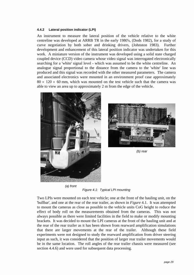
page 29
4.4.2 Lateral position indicator (LPI)
An instrument to measure the lateral position of the vehicle relative to the whitecentreline was developed at ARRB TR in the early 1980's, (Dods 1982), for a study ofcurve negotiation by both sober and drinking drivers, (Johnston 1983). Furtherdevelopment and enhancement of this lateral position indicator was undertaken for thiswork. A miniature version of the instrument was developed using a solid state chargedcoupled device (CCD) video camera whose video signal was interrogated electronicallysearching for a 'white' signal level - which was assumed to be the white centreline. Ananalogue signal proportional to the distance from the camera to the 'white' line wasproduced and this signal was recorded with the other measured parameters. The cameraand associated electronics were mounted in an environment proof case approximately80 × 120 × 60 mm, which was mounted on the test vehicle such that the camera wasable to view an area up to approximately 2 m from the edge of the vehicle.
(b) rear
(a) frontFigure 4.1: Typical LPI mounting
Two LPIs were mounted on each test vehicle; one at the front of the hauling unit, on the'bullbar', and one at the rear of the rear trailer, as shown in Figure 4.1. It was attemptedto mount the cameras as close as possible to the vehicle units CoG height to reduce theeffect of body roll on the measurements obtained from the cameras. This was notalways possible as there were limited facilities in the field to make or modify mountingbrackets. It was decided to mount the LPI cameras at the front of the hauling unit and atthe rear of the rear trailer as it has been shown from rearward amplification simulationsthat there are larger movements at the rear of the trailer. Although these fieldexperiments were not designed to study the rearward amplification from driver steeringinput as such, it was considered that the position of larger rear trailer movements wouldbe in the same location. The roll angles of the rear trailer chassis were measured (seesection 4.4.6) and were used for subsequent data processing.

page 30
Both LPI cameras were focused to produce a measuring range from the inside of thedriver side tyres to approximately 2 m from the driver side of the vehicle.
4.4.2.1 Calibration
To allow for the LPI camera attitude (lens distortions, different mounting heights andangles of focus) it was necessary to obtain in-situ calibrations for each camerainstallation on each test vehicle. This calibration established a relationship between theoutput of the LPI unit and the lateral distance of a white object from the camera.
To reduce time in the field spent during the calibration and testing, it was considereddesirable to develop a dynamic calibration procedure. This was conducted at ARRB TRduring the development of the LPI instrument. A white flat canvas hose approximately150 mm wide (a length of industrial fire hose) was placed on the pavement surface at anangle of 30° to the longitudinal axis (centre-line) of the roadway, as shown inFigure 4.2. Black stripes were painted every 1 m along the hose. The intention was todrive the test vehicle slowly (at walking pace), along the roadway and record the outputof the LPIs as the vehicle passed over the diagonal series of white section of the hose.The lateral position of the vehicle relative to the sections marked on the hose, could becalculated knowing the angle of the hose and the longitudinal position of the vehiclealong the centre-line.
Figure 4.2: Development of a dynamic LPI calibration method at ARRB TR
Several limitations of this calibration method were revealed during the development ofthe calibration procedure. The first limitation was measuring the lateral position of thevehicle as it passed along the calibration layout - the distance of the outside of thewheels from the centre-line. The second limitation was locating a suitable section ofroadway where a triple road-train could be manoeuvred (it was desirable to obtainrepeat passes for each calibration). The third limitation was locating a suitable sectionof roadway free of dirt (dry wheel tracks) that would give good contrast between theblack pavement surface and the white hose. The fourth and main limitation with thiscalibration procedure was that the longitudinal position of the vehicle could only beresolved to 750 mm which did not provide sufficient resolution for the calibration. The

page 31
longitudinal position resolution was subsequently increased to 250 mm. However,sufficient resolution could not be achieved and this technique was not pursued furtherand a static procedure was developed.
Figure 4.3: Field in-situ LPI calibration
The static calibration procedure was conducted by laying a length of black cloth on thearea of the pavement surface that the LPI camera scanned, and manually moving awhite plastic stick (150 mm × 2 m), away from the vehicle in 250 mm increments asshown in Figure 4.3.
The output of the LPI was recorded along with the incremental distance of the whitestick. Good repeatability was obtained with this static calibration procedure and repeatcalibrations were not necessary. Figure 4.4 shows typical recorded LPI calibrationdata. The plateaus represent the position of the white stick at each 250 mm lateralposition. The mean voltage was computed for the output at each lateral position and a5th order polynomial regression analysis was conducted to produce coefficients for thelateral distances against the position of the white stick. The coefficients from thisanalysis were used to convert the LPI recorded data into position of the test vehiclefrom centre-line.
A calibration was conducted for each LPI on each test vehicle.
-3
-2
-1
0
1
2
3
4
5
6
0 20 40 60 80 100 120 140 160 180 200Time (sec)
Output(v)
Figure 4.4: Recorded LPI calibration data

page 32
4.4.3 Lateral acceleration
High quality commercial accelerometers (±5 µg resolution) were used to measure thelateral acceleration at the longitudinal centre of gravity position of the vehicle units.Each accelerometer was mounted in an environment proof box (approximately 80 × 120× 60 mm) with a military specification connector which provided the connections tosupply the un-regulated power and the signal output. Regulated power supplies werecontained in each environment proof box, which provided isolation and reduced thepossibility of interference between signals. These accelerometers provide an electricalcurrent output which allows the transmission of outputs over long cables without loss ordegradation of the signal quality.
4.4.3.1 Calibration
All accelerometers were set to have a fixed measuring range of ±1 g (9.81 m/s/s).Calibration checks were conducted on each accelerometer by aligning theaccelerometer's sensitive axis vertical to the earth's axis and rotating the device 180°thus applying ±1 g force to the accelerometer. The accelerometer's output was recordedin both positions and the outputs were subsequently checked against the manufacturer'scalibration certificate.
4.4.4 Yaw rate
Yaw rate gyroscopes were mounted at the longitudinal centre of gravity position onboth the first and last vehicle units, ie. the hauling unit and the last trailer. Thesetransducers were mounted in the environment proof box with the accelerometers, wherethey obtained their power and signal connections.
4.4.4.1 Calibration
The yaw rate gyroscopes were set to have a fixed measuring range of ±45 deg/s.Calibrations were conducted in the laboratory by rotating the gyros through an angle of360° and recording the output against a known constant time base. The transduceroutputs were integrated against time, summed and divided by 360, thus producing acalibration constant expressed as deg/s/volts.
It was not practical to conduct calibrations for the yaw rate gyroscopes in the field,although operational checks were conducted as part of the vehicle instrumentationprocedures.
4.4.5 Steer wheel angles
The notion of instrumenting a vehicle to achieve the steer wheel angles, was to measurethe rotational position of both the driver and passenger side front wheels, using lineardisplacement transducers, and after conducting calibrations the rotational position of thesteer wheel angles was computed.
A 500 mm string linear displacement transducer was attached between the front axleand the wheel assembly on each side of the hauling unit to measure the rotationalposition of both steer wheels.
4.4.5.1 Calibration
The geometry for the steer wheel angles varied for each installation, hence a calibrationof the steer wheel angle transducers was necessary for each test vehicle.

page 33
Figure 4.5: A steer wheel calibration being conducted during another research program
This was achieved by attaching a pointer, as shown in Figure 4.5, to both the driver andpassenger side wheels on the front axle and rotating the steering wheel in half-turnincrements in both the clock and counter clockwise directions. The position of thepointer and the outputs of the transducers were recorded. Figure 4.6 shows typicalsensor outputs from a calibration. The labels above the plateaus on the plot indicate theposition of the steering wheel: 1 to 5 indicating the steering wheel rotations in half-turnincrements in the clockwise direction and 7 to 10 rotations in the counter clockwisedirection, label 6 is the straight-ahead position.
-800
-600
-400
-200
0
200
400
600
0 50 100 150 200
Time (sec)
Output(A/D Units)
Driver SidePassenger Side
1 2
3
4 5
6
7
8
910
Figure 4.6: Typical steer wheel transducer calibration output
The steer wheel angles were calculated with simple geometry from the position of thepointer, this information and the recorded transducer outputs were applied to a linearregression analysis to produced calibration coefficients. These coefficients were used toconvert the recorded displacement transducer outputs into driver and passenger sidesteer wheel angles. Correlation coefficients greater than 0.9 were computed for thesecalibrations with linear regressions, which means that the computed coefficientsexplained more than 90% of the calibration data.

page 34
4.4.6 Rear trailer chassis heights
The purpose of measuring the trailer chassis heights was to computed the trailer chassisroll angle. Non-contacting distance measuring transducers were mounted on each sideat the rear of the trailer chassis to measure the change in height (trailer roll) relative tothe pavement surface. These ultrasonic displacement transducers had a measuringrange of 200 to 1,500 mm. The mounting height and distance between the transducerswere noted for each vehicle as this was important information used when computing thechassis roll angles.
4.4.6.1 Calibration
A static calibration was conducted for each ultrasonic distance transducer before it wasmounted on the chassis. This calibration was achieved by mounting the transducer (atthe distance it would be from the pavement surface less 36 mm to allow for a calibrationpoint beyond where the pavement surface would be with the vehicle at rest) on acalibration rig, with the sensing axis pointing toward the ground as shown in Figure 4.7.Steel plates (6 mm thick) were added to reduce the measuring distance and the output ofthe transducer was recorded along with the number of plates.
Figure 4.7: Chassis height transducer field calibration rig
The recorded output from the displacement transducers and the number of plates waslater applied to a linear regression analysis, which produced calibration coefficients thatwere used to convert the recorded output into the height of each side of the trailerchassis. Table 4.1 shows the regression statistics for a typical regression analysis.

page 35
Table 4.1: Chassis height transducer – regression statistics
Regression Output:Constant 820.2Std Err of Y Est 2.4R Squared 0.98No. of Observations 87Degrees of Freedom 85X Coefficient(s) -153.6Std Err of Coef. 2.1
Figure 4.8 shows a typical output from a chassis height calibration. The 'Y' axis in thisFigure shows the transducer voltage output for the change in sensor measuring distance.The numbers above the step changes in Figure 4.8 show the distance of the sensor tothe target, in this case it can be seen that there was a 51 mm total change. Linearregression analysis produced correlation coefficients greater than 0.98 for thesecalibrations, which means that the computed coefficients explained more than 98% ofthe calibration data.
-1.0
-0.9
-0.8
-0.7
-0.6
-0.5
-0.4
0 10 20 30 40 50 60 70 80 90 100
Time (s)
Output(v)
919
910
925
931937
943949
955 961
Figure 4.8: Typical chassis heights calibration output
4.4.7 Rear axle motion (rear trailer)
Rear axle yawing information was collected for computer modelling and simulationvalidation, as it was thought that yawing of the rear axle would provide 'bump steer'input to the lateral movement of the trailer. Instrumentation to measure and record thisvehicle behaviour was developed.
Ultrasonic distance transducers (as shown in Figure 5.9) with a linear measuring rangeof 51 to 965 mm were mounted on each side of the rear axle of the last trailer. Thesewere focused onto aluminium plates that were fixed to the trailer chassis to provide areference position. These devices measured the movement of the rear axle in the 'X'(fore-aft) direction.

page 36
Figure 4.9: Transducers mounted to measure rear axle yawing
4.4.7.1 Calibration
A calibration procedure similar to the chassis height transducers, and subsequentregression analysis for these displacement transducers were conducted.
4.4.8 Articulation angle
A transducer was constructed to provide the articulation angle between the last twounits on the 'A' connected vehicles, ie. not the B-doubles. This transducer consisted of alinear potentiometric device with one end attached to chassis of the lead vehicle unitand the other end attached to the drawbar of the trailing unit.
4.4.8.1 Calibration
A calibration procedure (as shown in Figure 4.10) similar to the steer wheel angletransducers was conducted for each installation, and subsequent regression analysis forthe transducer outputs were conducted.
Figure 4.10: An articulation angle calibration during another research program
This calibration was conducted by manoeuvering the vehicle so the trailers were in astraight line - this was checked by a string line using the steer and drive tyres as the

page 37
reference. A number of data samples from the articulation transducers were recordedwith the vehicle at this straight-ahead position.
-150
-100
-50
0
50
100
150
0 5 10 15 20 25 30 35 40
Time (sec)
Output(A/D Units)
1
2
3
4
5
6
Figure 4.11: Typical articulation angle transducer calibration output
The vehicle was then manoeuvred to produce several angles of articulation between thelead and trailing units, these angles were computed using the geometry of the string-linemeasurements of the distance from the projected straight line to the vehicle chassis andthe length of the hypotenuse, see Figure 4.10. Figure 4.11 shows a typical articulationangle transducer recorded time history. The labels correspond to the articulation angleswhich were used for computing the calibration coefficients. There were only a limitednumber of points on this calibration due to the restricted area available to manoeuvrevehicles 36 m and 54 m long.
These computed angles and the recorded transducer outputs were applied to a linearregression analysis to produced calibration coefficients. These coefficients were used toconvert the recorded transducer outputs into the articulation angles of adjacent vehicleunits. Similar to the steer wheel angle measurements, correlation coefficients greaterthan 0.9, as shown in Table 4.2, were computed for these calibrations with linearregressions, which means that the computed coefficients explained more than 90% ofthe calibration data.
Table 4.2: Articulation angle transducer – regression statistics
Regression StatisticsMultiple R 0.99R Square 0.98Adjusted R Square 0.98Standard Error 1.16Observations 69
4.5 Data recordingA general purpose data logger that was developed at ARRB TR for heavy vehicle dataacquisition work was used to recording data in this study. The data logger was based ona commercial Dataq Inc. (Dataq 1993), unit which was housed in a case with signalconditioners, anti-aliasing filters and power supplies for the transducers. For these tests,

page 38
time based data samples of all 16 channels were written to a RAM file and saved to adisc file at the conclusion of the logging session. The ability for the experimenter toinput comments via the keyboard was a useful feature. These comments and theappropriate time from the start of the logging session were saved with the data and wereused when identifying or confirming the location of the test vehicle. The logger alsohas the ability to record digital information, this was used to record the longitudinalposition pulses obtained from the rotation of the vehicle tail-shaft. Power for the datalogger and transducers was obtained from the test vehicle's batteries.
The minimum sampling rates used in this study were 30 samples per second for the 16channels for the trailing fidelity tests and 80 samples per second for the rearwardamplification tests. The sampling rate of 30 samples/second was selected on the basisof ensuring 2 samples of the white centreline travelling at the maximum test speed,25 m/s (90 km/h). The centre-lines are generally 3 m long with 9 m gaps, and takingsamples every metre would ensure that the centreline was sampled. Given that thesampling was not synchronised to the occurrence of the centre-line, 30 samples/secondwas chosen to ensure sampling the centreline by covering variation in both the testvehicle speed and centreline spacing. The sampling was increased to 40 samples/s forsome of the test sections to ensure that the centreline was captured.
4.5.1 Data processing
All analogue data, except the LPI signals, were passed through eight order butterworthlowpass anti-alias filters prior to digitising, the cut-off frequencies of these filters wereset to 10 Hz which was below the nyquist frequency of 15 Hz. Digitising theory(Bendat & Piersol 1971) requires that the analogue signals to be digitised must notcontain energy (information) above the nyquist frequency, which is half of the samplingfrequency or distortions will be present in the recorded data.
A separate data file was created for each test section at each test speed for each vehicle,for subsequent analysis in the laboratory. A sample data file is shown in Appendix 7,Annex 1. During the data processing a number of outputs for each data file wereproduced. The prime output was a file containing the data from all recorded parametersconverted to engineering units. This was achieved by converting the recordedinformation from analogue/digital units into voltage and then applying the calibrationconstants to these voltage values to produce the data in engineering units. Two otheroutputs from the data processing were a file containing the comments entered by theresearcher during the data collection, and a file summarising the basic statisticalanalysis. The file containing the recorded comments also contained the followinginformation:
1) the time of day when the comments were entered;
2) the odo value;
3) the distance from the start of logging;
4) the vehicle speed when the comments were entered;
5) the total logging time;
6) the mean vehicle speed over the logging distance, which was determined by thetotal distance travelled divided by the logging time;
7) the logging distance.

page 39
A sample of this file is in Appendix 7, Annex 2. A sample of the summary statistics filewith the following statistics for all data channels; mean, standard deviation, RMS,maximum and minimum, skewness and kurtosis is in Appendix 7, Annex 3.
4.6 Pilot studyA pilot study to assess the suitability of the LPI transducers was conducted in April1995 using a truck-trailer combination. This vehicle was instrumented and road testswere conducted. This study proved to be invaluable in the context of the overallexperiment as it highlighted shortcomings in the data acquisition system. The majorshortcomings were as follows:
a) Prior to digitising (recording), all signals including the LPI signals were passedthrough low-pass anti-aliasing filters. This filtering process distorted thesesignals and reconstruction of the vehicle lateral position was not possible;
b) A high level of electrical interference from a power supply (used to power thenotebook computer) was present and induced noise on the data prior torecording.
Both of these important shortcomings were rectified prior to embarking on the fieldexperiments.
4.7 Data validationGiven the high cost to conduct this work and the experimental nature of these tests itwas important that the transducers were operating and measuring as expected and thatthe recorded data were valid. The test sections ranged in length from 700 to 1,400 mand sampling at 30 samples/sec, some of the data files contained up to 2,500 samplesper channel. Viewing 16 channels of data in these large data sets consumes valuabletime in the field. To provide visual data validation, a dedicated data plotting computerprogram was developed to enable data validation checks to be conducted graphicallyimmediately after the data were acquired.
This proved to be a useful tool for both the calibration and experimental data capture.
4.8 Field testing programThe dynamic road space requirement is a performance-based-measure, unlike othermeasures such as rearward amplification, which reflects relationships with the roadenvironment. It was therefore necessary to set-up the field testing measurementprogram to reflect such operating conditions. There are obviously practical limitationsto the extent of any testing program but the program developed was considered to be themost representative possible given the resources that could be made available.
4.8.1 Test vehicles
The test vehicles used for the first series of field experiments were selected to representa typical sample of the current vehicle fleet. Full vehicle details: dimensions and axleloads are given in Appendix 8, and Appendix 9 contains vehicle outline drawings.

page 40
Figure 4.12: A-triple, test vehicle 'C'
A brief description of the vehicles used for the first series of field experiments follows:
1) Single articulated, (A123), flat top trailer, 18 m long, steel suspension - coded asvehicle 'A';
2) A-double (A123-T23), flat top trailers, 33 m long, steel suspension - coded asvehicle 'B';
3) A-triple articulated (A123-T23-T23), flat top trailers, 48 m long, steel suspension -coded as vehicle 'C', (see Figure 4.12). The primer-mover and trailers shown inFigure 4.12 were also used for vehicles 'A' and 'B';
4) B-double (B1233), flat top trailers, 25 m long, tri-tri, steel suspension - coded asvehicle 'D', (see Figure 4.13);
5) B-double (B1232), flat top trailers tri-dual, 23 m long, air suspension - coded asvehicle 'E';
6) A-triple articulated (A123-T23-T23), car carrier, 49 m long, steel suspension -coded as vehicle 'F', (see Figure 4.14).
Figure 4.13: B-double, test vehicle 'D'
Table 4.3 shows the outline of test vehicles used for the first series of field experiments.
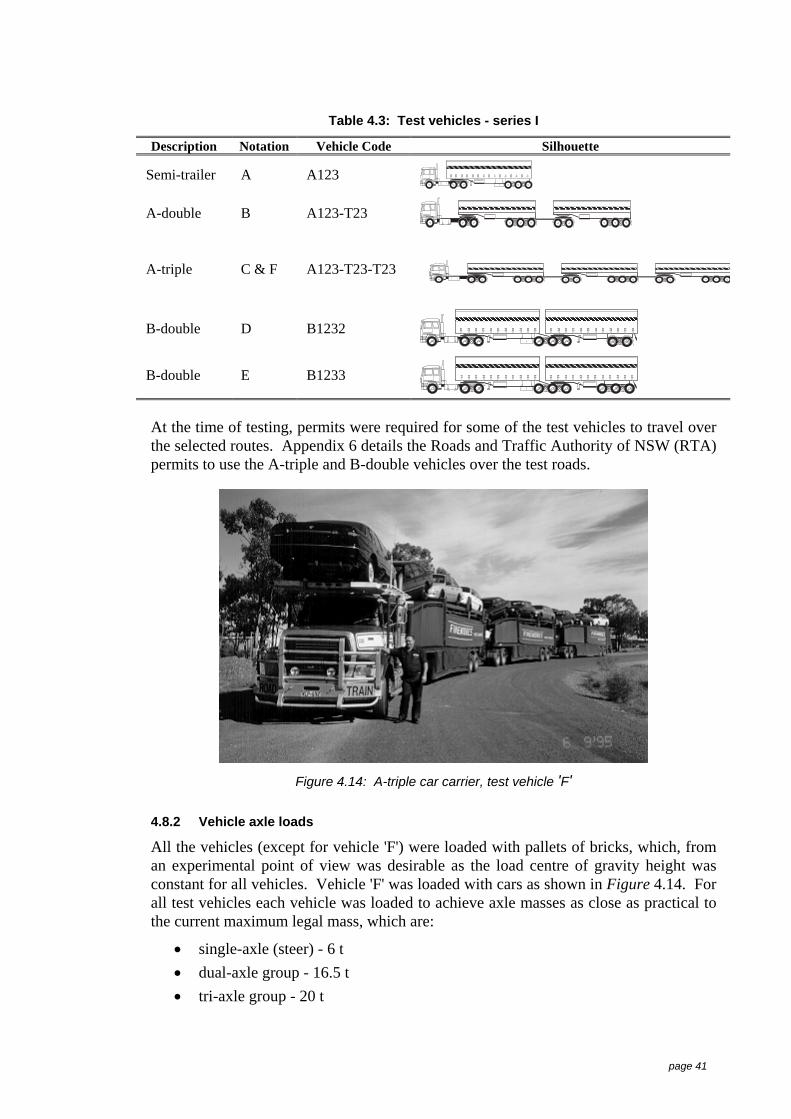
page 41
Table 4.3: Test vehicles - series I
Description Notation Vehicle Code Silhouette
Semi-trailer A A123
A-double B A123-T23
A-triple C & F A123-T23-T23
B-double D B1232
B-double E B1233
At the time of testing, permits were required for some of the test vehicles to travel overthe selected routes. Appendix 6 details the Roads and Traffic Authority of NSW (RTA)permits to use the A-triple and B-double vehicles over the test roads.
Figure 4.14: A-triple car carrier, test vehicle 'F'
4.8.2 Vehicle axle loads
All the vehicles (except for vehicle 'F') were loaded with pallets of bricks, which, froman experimental point of view was desirable as the load centre of gravity height wasconstant for all vehicles. Vehicle 'F' was loaded with cars as shown in Figure 4.14. Forall test vehicles each vehicle was loaded to achieve axle masses as close as practical tothe current maximum legal mass, which are:
• single-axle (steer) - 6 t• dual-axle group - 16.5 t• tri-axle group - 20 t

page 42
It should be noted that it was not possible to adjust the axle load for vehicle 'F'. Toensure the axle masses were close to the legal limits all vehicles were weighed and theload adjusted as required. Figure 4.15 shows a Traffic Officer weighing a test vehiclewith portable scales.
Figure 4.15: Traffic Officer weighing a test vehicle
4.8.3 Test speeds
In selecting the range of speeds for the vehicles to traverse the test roads, a number ofpractical factors were considered. Firstly, if the effect of speed was to be obtained fromthe experiment, then it was desirable to conduct the test at the widest range of speedspossible. Secondly, the largest vehicle type tested, the triple road-train, had a maximumgeared speed of 90 km/h, therefore 90 km/h was selected to be the maximum test speed.The final consideration was the integration of the test vehicle into the traffic flow, as thetest roads were rural two-way with speed limits of 100 km/h, the minimum test speedwas selected to be 60 km/h.
The nominal test speeds were therefore selected to be: 60, 75 and 90 km/h.
4.8.4 Test roads
One of the aims of this work was quantifying the influence of pavement characteristicson the lateral movement and hence the road space requirements of vehiclecombinations. In order to obtain an understanding of the effects of the various levels ofpavement roughness on vehicle lateral movement, pavement segments with a range ofroughnesses were selected for the tests.
4.8.4.1 General pavement condition indicators
Pavement condition is generally classified by a roughness index, which is a quantitativesummary of the pavement surface variations. State road authorities in Australia havetraditionally classified pavement surface condition with a NAASRA Roughness meter10.This is a mechanical device connected to a passenger car that registers the relativevertical displacement between the vehicle's rear axle and a point on the vehicle's body
10 Laser-based profile measuring equipment has now largely replaced the use of the NAASRA Roughness
Meter, however relationships have been developed between the NAASRA and IRI indices, (Prem1989a), (see Table 4.3).

page 43
vertically above the axle, Scala and Potter (1977). The International Roughness Index(IRI) is also a pavement surface condition indicator, it summarises the roughnessquantities that impact passenger vehicle response, and is a measure of the verticalresponse to the pavement profile of a quarter-car model travelling at 80 km/h. Thequarter-car model which was developed by Sayers (1995) filters the profile frequencycomponents which have little effect on the ride quality experienced by the car. The IRIindex was developed by Sayers et al, (1986) with the view to providing an internationaltime-stable, easily transportable and reproducible pavement condition measure.
The IRI is an overall pavement surface indicator index and has units of mm/m or m/km.It is used for a range of vehicle/road studies such as vehicle operating costs, ride qualityand dynamic wheel loading.
The IRI index is an open-ended scale: a value of 0 is a perfectly flat surface scale and 8would be an unpaved surface or severely damaged pavement. Figure 4.16 gives anindication of the IRI ranges for different pavement conditions. It should be noted thatthe information presented in Figure 4.16 represents a wide IRI range for each segmentand could be based on theoretical assessment not from measured pavements.Furthermore, the travel speeds listed are assumed to be for passenger vehicles not heavyvehicles.
0
2
4
6
8
10
12
14
16
18
20IRI
(m/km)
Speed of normal use(km/h)
30
50
60
80
100
0 = absolute perfection
airport runwaysand superhighways
older pavements
surface imperfections
maintained unpaved roads
new pavements
damaged pavements
rough unpaved roads
erosion gulleys and deep depressions
frequent shallow depressions, some deep
frequent minor depressions
source: Sayers and Karamihas (1996b)
Figure 4.16: IRI ranges for different pavement conditions
Due to the large differences in pavement conditions in the state/territories throughoutAustralia, there are no common standards for expressing the serviceability of roadsusing the NAASRA or IRI index.
Information collected on the roughness levels on rural roads throughout Australia(Table 4.4) showed that generally, except for Queensland, around one third of theproportion of rural roads had roughness levels greater than IRI 4 (NRM 110 c/km).

page 44
Table 4.4: Australian rural lane-km pavement roughness
Proportion of rural lane-km with roughness > IRI 4
Road TypeNorthernTerritory Queensland South
AustraliaWesternAustralia Victoria
National Highway 2 9 1 4 3State Highway 6 17 7 5 7
Secondary 7 21 10 4 14Local 8 32 8 5 11
TOTAL (%) 23 79 26 18 35source: Information collected via a telephone survey conducted by ARRB TR 2001
Notes:1. Road types were not consistent between the jurisdictions and four categories are used here
for the purposes of illustration.2. The data were collected in NAASRA roughness units (NRM 110 c/km).3. Data not available for New South Wales.4. Data not collected for Tasmania.
The pavement roughness levels and serviceability levels shown in Table 4.5 are putforward for classifying roads for this work. It should be noted that the descriptors'smooth', 'medium' and 'rough' refer to the rideability of passenger cars over roads withthese roughness characteristics: they may not be an appropriate description for heavyvehicles. However, with no other means of quantifying or classifying roads for heavyvehicle response at the time of conducting the field experiments, these rankings wereused as a selection criterion for the test roads for this work.
Table 4.5: Pavement roughness classification
Roughness Index Serviceability DescriptionNAASRA
(counts/km)IRI
(m/km)
< 60 < 2.3 New construction Smooth
60 - 100 2.3 – 3.8 Freight routes Medium
> 100 > 3.8 Requires maintenance Rough
4.8.4.2 Selecting test roads
There were a number of desirable requirements for the selection of the test roads.Primarily, as the pavement unevenness or roughness provided the 'input' to the vehiclesystem it was imperative that the test roads represented a range of freight routesthroughout Australia.
For this test program it was desirable that the test roads had 'straight sections' ofsufficient length to allow representative performance data to be acquired. This wasimportant as the experiment was designed to obtain the lateral movement of the vehiclesduring straight-ahead travel, with minimum steering wheel activity. Excessive steeringactivity could induce lateral movement at the rear trailer which is not directly related tovehicle speed or pavement condition. As a result, 'noise' could be introduced into thedata which could influence the outcomes of the study.
Another important requirement when selecting the roads for the first series ofexperiments was that there were no light coloured stones or particles in the pavementsurface and that the white centreline provided good contrast with the pavement surface.The LPI relied on the centreline to provide a 'high' colour contrast from the pavement.

page 45
Both these characteristics were important if the video-based lateral position instrument(LPI) was to give reliable data. A pavement surface free from shadows was alsoimportant, as the camera in the LPI utilised an auto-iris lens which could not respond tolarge changes in lighting conditions when travelling at 25 m/s (90 km/h) throughintermittent shadows.
The ability to manoeuvre and make 'U' turns with a long combination vehicle,approximately 50 m long, and achieve the 90 km/h maximum test speed were alsorequirements. Roads with low traffic flows were also sought as testing at the low speedwould possibly cause queuing, potentially presenting an unsafe environment. Slowvehicles encountered, especially during the high-speed testing, may have interfered withthe desire to maintain a constant speed.
The final requirement was from a practical viewpoint, that the test sections be locatedwithin close proximity of each other to reduce unnecessary time and travel between testsections.
As would be expected, not all the above requirements for test roads could be met.Nevertheless, test roads were located west of Parkes NSW between Yarrabandai andCondobolin, with an approximately route length of 60 km. Figure 4.17 shows thelocation of the test sections. All were approximately one kilometre in length.
Figure 4.17: Location of the test roads
As part of determining the test roads for this work a number of sections were identifiedfrom the high-speed roughness surveys. Using the pavement classification as shown inTable 4.5, two sections for the smooth, medium pavement conditions and three sectionsfor the rough condition were identified. The section within each pavement conditionwere arbitrarily named sections 'A', 'B' and 'C'. During the series I experiments datawere recorded over all the identified sections, however, in general only one smooth,medium and rough section were used during data analysis. The test sections werecoded as follows: 'S' Smooth, 'M' Medium and 'R' Rough, section 'A', 'B' or 'C' and 'E'east or 'W' for west bound. The following sections were used for this work:
Smooth – section 'A' east bound (SAE), located on the Parkes Condobolin Road,

page 46
82.37 km west from Welcome Street Parkes.
Medium – section 'B' east bound (MBE), located on the Parkes Condobolin Road,79.37 km west from Welcome Street Parkes.
Rough – section 'C' west bound (RCW), located on the Parkes Condobolin Road,75.60 km west from Welcome Street Parkes.
To identify the start and end of each test section used during the field experiments,marks were painted on the pavement at these locations. These marks allowedidentification of the sections from the vehicle, via the experimenter comments that wererecorded with the measured data.
4.8.4.3 Pavement surface characterisation
A high-speed Profiler to measure pavement profile was developed at ARRB TR, Prem(1989b). This Profiler is an instrumented vehicle using laser-based equipment tomeasure pavement surface shape at highway speed. The high-speed Profiler was usedto measure the profiles of a number of roads prior to the commencement of the fieldexperiments in the driver and passenger heavy vehicle wheelpaths (1.8 m spacing). Inorder to estimate the pavement crossfall, a reference between the passenger and driverwheel path profiles is required. Unfortunately it was not possible to obtain thisreference for profiles measured with the high speed Profiler.
Prior to the second series of experiments a selection of the same test roads weremeasured with the ARRB TR Walking Profiler, ARRB TR (1995). This device canaccurately measure the absolute profile of a surface to an accuracy of ±1 mm over 50 m.Pavement profiles were measured in the two heavy vehicle wheel paths with theWalking Profiler using the same initial reference point. In addition, to ensure the wheelpath profiles contained true crossfall information, lateral measurements between the twowheel paths were taken every 100 m and were used to compute the crossfallrelationship.
Figure 4.18 shows a plot of the raw profile data for the passenger and driver wheelpaths for the ‘medium’ roughness test section taken in the east bound direction. Bothprofiles have the same initial starting reference point and have not been corrected forcrossfall.

page 47
-0.2
0.0
0.2
0.4
0.6
0.8
1.0
0 100 200 300 400 500 600 700 800 900 1,000
Distance (m)
Profile(m)
DriverPassenger
Figure 4.18: Passenger and driver wheel path profiles - MBE
Figure 4.19 shows the same profile information as presented in Figure 4.18 withcorrection for the measured crossfall.
This wheel track profile information was retained and used as a vehicle disturbanceinput during the vehicle lateral movement computer simulation.
-0.2
0.0
0.2
0.4
0.6
0.8
1.0
0 100 200 300 400 500 600 700 800 900 1,000
Distance (m)
Profile(m)
DriverPassenger
Figure 4.19: MBE wheel path profiles corrected for crossfall
On ‘real’ roads the crossfall will vary along a length of pavement due to factors such asvariability in construction materials and deterioration. The point-by-point crossfallvalues were computed for the test sites from the difference in the driver and passengerwheelpath profiles, using the same initial reference point. Figure 4.20 shows thecomputed crossfall for the MBE test road. The mean crossfall value is computed to be –4.5%, the sign indicating the fall is away from the centre line.
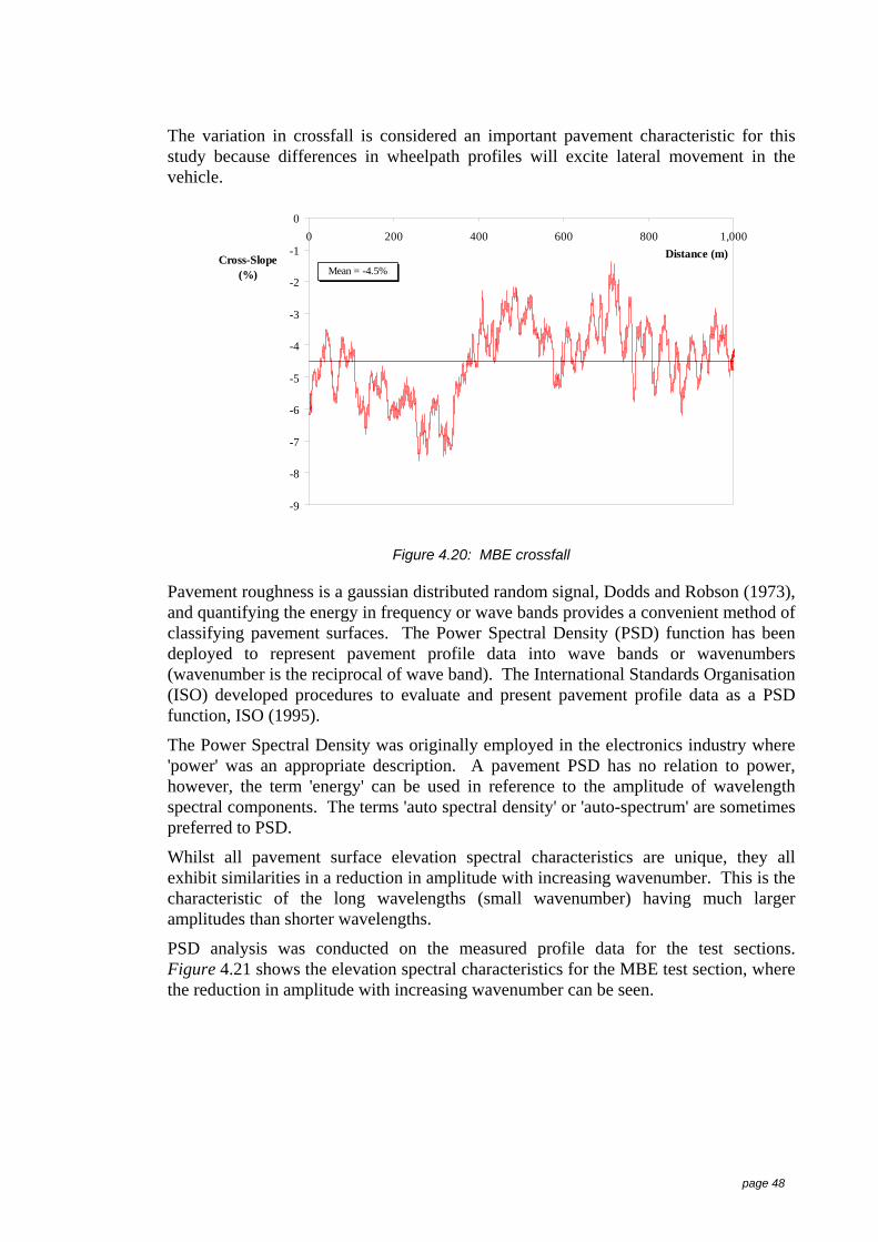
page 48
The variation in crossfall is considered an important pavement characteristic for thisstudy because differences in wheelpath profiles will excite lateral movement in thevehicle.
-9
-8
-7
-6
-5
-4
-3
-2
-1
00 200 400 600 800 1,000
Distance (m)Cross-Slope(%) Mean = -4.5%
Figure 4.20: MBE crossfall
Pavement roughness is a gaussian distributed random signal, Dodds and Robson (1973),and quantifying the energy in frequency or wave bands provides a convenient method ofclassifying pavement surfaces. The Power Spectral Density (PSD) function has beendeployed to represent pavement profile data into wave bands or wavenumbers(wavenumber is the reciprocal of wave band). The International Standards Organisation(ISO) developed procedures to evaluate and present pavement profile data as a PSDfunction, ISO (1995).
The Power Spectral Density was originally employed in the electronics industry where'power' was an appropriate description. A pavement PSD has no relation to power,however, the term 'energy' can be used in reference to the amplitude of wavelengthspectral components. The terms 'auto spectral density' or 'auto-spectrum' are sometimespreferred to PSD.
Whilst all pavement surface elevation spectral characteristics are unique, they allexhibit similarities in a reduction in amplitude with increasing wavenumber. This is thecharacteristic of the long wavelengths (small wavenumber) having much largeramplitudes than shorter wavelengths.
PSD analysis was conducted on the measured profile data for the test sections.Figure 4.21 shows the elevation spectral characteristics for the MBE test section, wherethe reduction in amplitude with increasing wavenumber can be seen.

page 49
1.E-08
1.E-06
1.E-04
1.E-02
1.E+00
0.001 0.010 0.100 1.000 10.000Wave number (cycle/m)
PSDof Elevation (m^3/cycle)
PassengerDriver
Figure 4:21: Elevation spectral characteristics - MBE
The slope PSD best shows differences in roughness properties, because the elevationspectrum of roughness over wave number is more uniform. ie., the roughnessamplitudes change less over the waveband of interest.
Sayers and Karamihas (1996a) explain the advantages of using the slope PSD toidentify the variation in profile wavebands:
"The PSD of profile elevation at low wavebands is numerically much larger thanthe amplitude associated with high wavebands. The large difference in amplitudecan complicate statistical analyses because side effects of the numerically largevalues mask the significance of the smaller values. In contrast the slope PSD isfairly uniform over the entire range of wave numbers, covering just one order ofmagnitude."
Figure 4.22 shows the slope spectral characteristics for both the driver and passengerwheelpath profiles on the MBE road. It can be seen from this Figure that the peak forboth wheel paths are around 0.007 wavenumber, which is a wave length of 145 m. Atthis peak the passenger and driver plots are identical and as shown in Figure 4.22, theheavier passenger line covers the lighter driver plot.

page 50
1.E-06
1.E-05
1.E-04
1.E-03
0.0001 0.0010 0.0100 0.1000 1.0000 10.0000Wave number (cycle/m)
PSD of Slope(m/cycle) Driver
Passenger
Figure 4.22: Slope spectral characteristics - MBE
Table 4.6 lists the summary information for test sections; IRI, the mean crossfall andstandard deviation (σ), and the mean square value of profile height. The mean square ofprofile elevation is the average value of all the squared profile height data. The meansquare value is the integration of all frequencies (the sample variance), and is also equalto the total area under the auto spectral density. The profile mean square covers the fullwavelength range and is a measure of the potential total energy that could betransmitted from the pavement surface to the vehicle. On the other hand, IRI is ameasure of rideability in a passenger car and may not provide an appropriate measurefor heavy vehicle response. Studies by McLean and Ramsay (1996), McManus et al(1998) and Hassan and McManus (2000) have concluded that heavy vehicles respond topavement profile wavelengths differently than passenger vehicles, and haverecommended that a ride index be developed for heavy vehicles.
It is of interest to note for the MBE road, the larger value in mean square for the driverprofile than the passenger profile, whilst the passenger IRI value is larger. This may bedue to the bandpass filtering characteristics of the quarter car model that is used toestimate the IRI index, which may not be responding to dominant spectralcharacteristics of the pavement.
Table 4.6: Test road characteristics
Mean Roughness Profile elevationTest Lane Passenger Driver Passenger Driver Crossfall
Section Length Width IRI Mean Square Lane IRI Mean SD(m) (m) (m/km) (m2 × 103) (m/km) (%)
SAW 1,200 3.9 2.99 3.00 1.39 1.31 3.00 -3.03 0.56SAE 1,200 3.8 2.92 3.00 1.77 1.68 2.96 -3.19 0.98MBE 1,000 3.6 4.31 3.84 1.78 2.45 4.08 -4.49 1.18MBW 1,000 3.6 3.47 3.13 3.49 3.50 3.30 -4.22 0.99RCW 1,000 2.9 4.38 4.52 3.81 4.15 4.45 -4.00 0.68RCE 1,000 2.7 5.90 5.13 9.68 2.83 5.51 -3.20 2.48
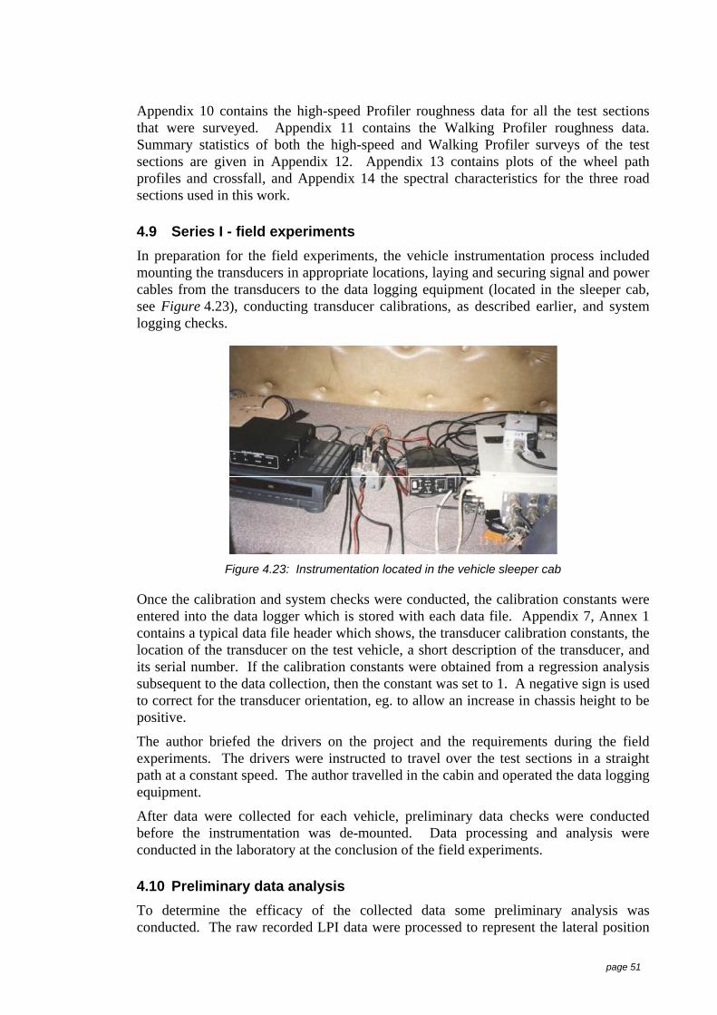
page 51
Appendix 10 contains the high-speed Profiler roughness data for all the test sectionsthat were surveyed. Appendix 11 contains the Walking Profiler roughness data.Summary statistics of both the high-speed and Walking Profiler surveys of the testsections are given in Appendix 12. Appendix 13 contains plots of the wheel pathprofiles and crossfall, and Appendix 14 the spectral characteristics for the three roadsections used in this work.
4.9 Series I - field experimentsIn preparation for the field experiments, the vehicle instrumentation process includedmounting the transducers in appropriate locations, laying and securing signal and powercables from the transducers to the data logging equipment (located in the sleeper cab,see Figure 4.23), conducting transducer calibrations, as described earlier, and systemlogging checks.
Figure 4.23: Instrumentation located in the vehicle sleeper cab
Once the calibration and system checks were conducted, the calibration constants wereentered into the data logger which is stored with each data file. Appendix 7, Annex 1contains a typical data file header which shows, the transducer calibration constants, thelocation of the transducer on the test vehicle, a short description of the transducer, andits serial number. If the calibration constants were obtained from a regression analysissubsequent to the data collection, then the constant was set to 1. A negative sign is usedto correct for the transducer orientation, eg. to allow an increase in chassis height to bepositive.
The author briefed the drivers on the project and the requirements during the fieldexperiments. The drivers were instructed to travel over the test sections in a straightpath at a constant speed. The author travelled in the cabin and operated the data loggingequipment.
After data were collected for each vehicle, preliminary data checks were conductedbefore the instrumentation was de-mounted. Data processing and analysis wereconducted in the laboratory at the conclusion of the field experiments.
4.10 Preliminary data analysisTo determine the efficacy of the collected data some preliminary analysis wasconducted. The raw recorded LPI data were processed to represent the lateral position

page 52
of the driver side tyre of the test vehicle to the centreline. Details of the data processingprocedures for the LPI data are given in the following Chapter.
After the LPI data was processed into position information, summary statistics (mean,σ, maximum and minimum, skewness and kurtosis) were computed for all signals. (seeAppendix 7, Annex 2 for a sample summary statistics file).
An in-depth analysis was conducted on the A-triple (vehicle 'C') to determine therelationships between the road roughness and vehicle speed as the independentvariables (IV), and the lateral position as the dependent variable (DV). Data recordedover the twelve measured test sections were used for this analysis. The standarddeviation of the lateral position was used as the dependent variable because thevariation about the mean lateral position is an indication of the lateral movement of thevehicle. Also the standard deviation can be used as a measure to compare relativeperformance between vehicle types.
This investigation between the dependent variable and pavement roughness revealedthat no linear relationship existed. The correlation coefficient (r2) was less than 3×10⁻⁵
- which means that less than 0.003% of the variation in lateral position can be explainedby the variation in roughness. Similarly no correlation was found between lateralposition and vehicle speed.
Sweatman (1983) found a strong correlation between speed times the square root ofpavement roughness (VSR) and heavy vehicle pavement loading. Combining vehiclespeed and pavement roughness in this manner provided a convenient method of usingthe two parameters that were the control variables for this study during the preliminaryanalysis. This new independent variable was used to investigate relationships withvarious measured vehicle parameters.
A number of linear correlations were conducted to identify the relationships betweenthe independent and dependent variables. Table 4.7 shows the relationships betweenpavement roughness, VSR and a selection of measured variables for the tripleroad-train, vehicle 'C'.
No correlation was found between VSR and lateral position - a correlation coefficient(r2) less than 0.02. After an exhaustive manipulation and investigation into the lateralposition signals it was concluded that the LPI lateral position signals did not accuratelyrepresent the dynamic lateral position of the vehicle relative to the centreline and furtheruse of these data was abandoned.
As the processing and analysis of the LPI signals were found not to provide the lateralposition of the test vehicles suitable for rigorous analysis, another method of measuringthe lateral position using a water trace and a video camera mounted on the rear of thevehicles was developed and subsequently used for the second series of field tests.

page 53
Table 4.7: Correlations for vehicle 'C'
Measure(SD) Independent variable Relationship
Correlationcoefficient
(r2)
Lateral positionrear unit
Pavement roughness Very weak 0.00003
Lateral positionrear unit
VSR Very weak 0.017
Yaw rate - front VSR Very weak 0.087
Yaw rate - front Pavement roughness Weak 0.123
Steering activity VSR Weak 0.230
Steering activity Pavement roughness Mild 0.412
Lateral accelerationfront unit
VSR Mild 0.440
Lateral accelerationrear unit
Pavement roughness Mild 0.485
Yaw rate - rear Pavement roughness Mild 0.495
Lateral accelerationfront unit
Pavement roughness Mild 0.561
Yaw rate - rear VSR Strong 0.718
Lateral accelerationrear unit
VSR Strong 0.776
Figure 4.24 shows the lack of correlation between the standard deviation of lateralposition and VSR, a very high constant (116) and extremely small coefficient (0.18)which means that there is a low predictive power as the constant dominates thepredicted values. This Figure also shows the measured values are distributed randomlyaround the predicted values, which is essentially a straight line. The reason for thisweak correlation was not known but it is assumed to be a function of the LPI measuringdevices.
Although the data from the LPIs were deemed as not adequate for the prime datasource, some LPI data were extracted and presented in Chapter 7.
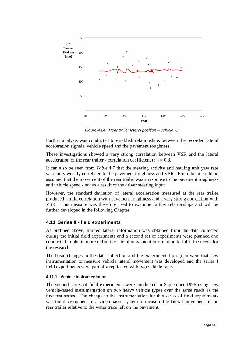
page 54
0
50
100
150
200
250
50 70 90 110 130 150 170
VSR
SDLateralPosition
(mm)
Figure 4.24: Rear trailer lateral position – vehicle 'C'
Further analysis was conducted to establish relationships between the recorded lateralacceleration signals, vehicle speed and the pavement roughness.
These investigations showed a very strong correlation between VSR and the lateralacceleration of the rear trailer - correlation coefficient (r2) = 0.8.
It can also be seen from Table 4.7 that the steering activity and hauling unit yaw ratewere only weakly correlated to the pavement roughness and VSR. From this it could beassumed that the movement of the rear trailer was a response to the pavement roughnessand vehicle speed - not as a result of the driver steering input.
However, the standard deviation of lateral acceleration measured at the rear trailerproduced a mild correlation with pavement roughness and a very strong correlation withVSR. This measure was therefore used to examine further relationships and will befurther developed in the following Chapter.
4.11 Series II - field experimentsAs outlined above, limited lateral information was obtained from the data collectedduring the initial field experiments and a second set of experiments were planned andconducted to obtain more definitive lateral movement information to fulfil the needs forthe research.
The basic changes to the data collection and the experimental program were that newinstrumentation to measure vehicle lateral movement was developed and the series Ifield experiments were partially replicated with two vehicle types.
4.11.1 Vehicle instrumentation
The second series of field experiments were conducted in September 1996 using newvehicle-based instrumentation on two heavy vehicle types over the same roads as thefirst test series. The change to the instrumentation for this series of field experimentswas the development of a video-based system to measure the lateral movement of therear trailer relative to the water trace left on the pavement.

page 55
In addition to the video based lateral movement device, to satisfy the aims and needs forthis research, a number of other vehicle parameters were also recorded during thesetests. The test vehicles in the second series field experiments were instrumented tomeasure the following vehicle parameters:
a) Forward distance travelled;
b) Lateral movement of the rear of the last trailer relative to the position of thehauling unit front;
c) Lateral acceleration of each vehicle unit, measured at the longitudinal centre ofgravity;
d) Rear trailer chassis heights (roll angle);
e) Yaw rate of the front and rear vehicle units at the longitudinal centre of gravity.
The same signal instrumentation and data logging equipment that was used for the firstfield experiments was used for this series of experiments. Data sampling frequencies of10 or 20 Hz were used to acquire data for these field experiments.
4.11.2 Video-based lateral movement measurement
A video-based system was developed to record the lateral movement of the rear of thevehicle relative to the front of the vehicle. A water nozzle aimed at the ground wassecured to the steer axle of the hauling unit, (Figure 4.25). This arrangement left a traceof the vehicle's path on the pavement as shown in Figure 4.26.
Figure 4.25: The water nozzle mounted at the front of the test vehicle
A video camera mounted on the rear of the vehicle (see Figure 4.27) was aimed at thepavement, recorded an image of the pavement showing the water trace. The location ofthe water trace in the video images was used to estimate the lateral position of the rearof the vehicle relative to the hauling unit (prime mover).

page 56
Figure 4.26: A water trace showing the vehicle relative movement
(b) A video camera mounted on the rear of atest vehicle
(a) A video camera and chassis height
Figure 4.27: Sensor mounted on the rear of the test vehicles
4.11.2.1 Calibration
Similar to the LPI video camera, the attitude (lens distortions, different mountingheights and angles of focus) of the video camera influence the proportion of therecorded images. Accordingly, for this application, in-situ calibrations for each camerainstallation on each test vehicle were required.
video camera

page 57
This calibration procedure involved drawing a grid of known dimensions on thepavement (see Figure 4.28) and recording an image of this grid. Prior to the extractingthe lateral movement data from the recorded water trace image, a set of screen to realco-ordinates are computed and these were used to convert the water trace position intoengineering units.
Figure 4.28: Development of the video calibration procedure at ARRB TR
Given the nature of the instrumentation, a process to validate the operation of the video-based lateral measurement system was conducted using the vehicle shown inFigure 4.28.
4.11.3 Test vehicles
The vehicles used for the second test series are as outlined in Table 4.8 and describedbelow:
1) A-double (A123-T23), steel suspension, 33 m long - coded as vehicle 'G', loadedwith grain, Figure 4.29;
2) Truck-trailer (R12 T12), steel suspension, 17 m long - coded as vehicle 'H', wasloaded with sand, Figure 4.30.
Table 4.8: Test vehicles - series II
Description Notation Vehicle Code Silhouette
A-double G A123-T23
Truck-trailer H R12-T12

page 58
Figure 4.29: A-double, test vehicle 'G'
The test speeds and roads sections used for series II experiments were the same as usedfor series I experiments. As there was sufficient time available and vehicle 'H' wascapable of travelling at 100 km/h it was decided to collect data at this speed.
Figure 4.30: Truck-trailer, test vehicle 'H'
4.12 Summary of the experimental programSeries I
Six test vehicles (one single articulated, one A-double, two A-triples and two B-doubles) were all driven over 6 test sections of measured pavement roughness. The testsections were classified as ‘smooth’, ‘medium’ and ‘rough’ based on their IRIroughness values. Data were recorded in both the west and east-bound directions.Although all data were converted to engineering units and processed only one testsection for each pavement classification was selected for data analysis. These werebased on the sections with the most complete data sets.
The nominal test speeds were chosen to be 60, 75 and 90 km/h. The vehicle speedsalong with up to 16 channels of vehicle data were recorded.
Series II
Two test vehicles were used for the second series of field experiments: one A-doubleand one truck-trailer combination. The same vehicle speeds and test sections were usedfor these experiments. Similar to the first series data were recorded over 6 test sectionin both the west and east-bound directions. A different set of measurements were madeon these test vehicles than on the first series. A number of replication passes were madeover each pavement test section.

page 59
4.13 SummaryTo meet the need for the lateral performance information of heavy vehicles as identifiedfrom the literature review and the needs of the state and national bodies, anexperimental design and program were developed. A comprehensive set of vehicleinstrumentation was developed to collect the vehicle lateral performance data for theseneeds.
Analysis of the data collected from the first series of field experiments showed that thelateral position as measured by the LPI device did not provide data to enable strongrelationships between the control variables and the lateral position of the vehicle to befound. A second set of field experiments was subsequently developed and conducted toobtain more definitive lateral movement information.
Data processing and subsequent analysis for data collected in both field experimentswill be discussed in the following Chapters.

page 60
5 Data Processing and Supplementary Information
5.1 IntroductionIn the previous Chapter the field data collection was described. This Chapter outlinesthe procedures that were developed to extract the lateral position information from therecorded information from the series I field experiments, and the lateral movementinformation from the information recorded from the series II field experiments. Theprocessing of the rearward amplification information, and the method used to estimatelateral movement from the measured lateral acceleration and trailer chassis heightmeasurements are also described in the Chapter.
Substantial effort was focused on processing the recorded outputs from the LPItransducers to extract the vehicle lateral position information relative to the centreline.Several methods of converting the recorded information and data analysis wereattempted before it was decided that this information would not satisfy the needs of thestudy, and the second series of field experiments were conducted using new purpose-built lateral movement measuring equipment. The processing of this data is alsodiscussed in this Chapter.
During the series I field experiments articulation angles between vehicle units, and therear axle motions were measured and recorded for all vehicles. These data wereintended to provide an input into computer simulation validation, however, as the datawere not used for the validation it was not processed and therefore is not reported here.
5.2 LPI dataThe LPI signals were processed from the raw recorded signals to represent the lateralposition of the test vehicle from the pavement centre-line. As mentioned in theprevious Chapter, (in the pilot study) the LPI signals were not passed through low-passfilters to preserve their high frequency components. The LPI signals were a pulsesignal with very high rise times, which means that they contain very high frequencies,and if these high frequencies were filtered then the shape and amplitude would havebeen distorted making the extraction of the lateral position of the centreline inaccurate.
-5
-4
-3
-2
-1
0
1
2
3
0 10 20 30 40 50 60
time (sec)
Output(v)
Figure 5.1: Typical LPI signal time history

page 61
Figure 5.1 shows a time history for a typical LPI signal. The lateral position of thevehicle from the centreline is contained in the amplitude of each valid spike.
It can be seen in Figure 5.1 that some spikes over-shoot and some do not contribute tothe general signal shape. These 'false' signals (see item 2 below) are attributed to whiteor reflective material or particles in the pavement surface that produce a return signalin-between the centrelines or when they are not detected.
The following steps outline the procedure that was developed to process the LPI data toextract the position of the test vehicle from the centreline:
1) Determine the noise or 'black' level of the signal - this was achieved by computingsummary statistics on the raw data, and setting a threshold level based on 75 % ofthe minimum level above the black level.
2) Determine the 'false' return signal. A false signal was represented as highfrequency (sharp rise pulses) in the data stream which were deemed to represent anunrealistic level of lateral movement of the vehicle. These high frequency pulsescan be seen in Figure 5.2 to extend above the estimated position.
3) Interpolate between the centreline measurements - effectively joining the datapoints between valid returned signals from the centre-lines. This was achievedusing a linear fit between the two valid measured points.
4) Apply the coefficients obtained from the in-situ calibrations to the LPI transducersand apply a smoothing function to the joined points.
Figure 5.2 shows typical LPI processed data which has been smoothed to extractcontinuous position information. The 'false' return signals have effectively beenremoved by the smoothing process.
-5
-4
-3
-2
-1
0
1
0 10 20 30 40 50 60 70
time (sec)Output(v)
Figure 5.2: Lateral position and smoothed overlay plot
LPI data recorded from vehicle 'C' were processed as described above and analysed asreported in the previous Chapter.

page 62
As shown in the previous Chapter, using the processing procedures developed here, nolinear relationship could be established between the LPI position information and anumber of independent variables. After considerable data processing and analysis wereconducted using the LPI lateral position information, no linear relationships could beestablished between the lateral position data and the control variables. Consequently itwas decided to abandon further analysis using this lateral position information.
Notwithstanding the above, LPI lateral position data for vehicles 'B' and 'C' wereconsidered to contain some useful information and this data is presented and analysed inChapter 7.
5.3 Lateral acceleration dataAs shown in the previous Chapter (Table 4.7) a strong linear relationship wasestablished between lateral acceleration and the independent variable speed times thesquare root of pavement roughness (VSR). In addition further analyses were conductedusing the measured lateral acceleration data.
5.3.1 Tests for lateral acceleration normality
To determine the reliability and robustness of statistical assumptions using the lateralacceleration a discrete probability density function was computed on the measured data.The lateral acceleration data that was measured at the rear of the last trailer on vehicle'B' over the MBE road at the nominal speed of 60 km/h, was used to compute thisfunction. There were 1900 data samples in this time history. Figure 5.3 shows thisfunction plotted over the normal distribution function. It can be seen in this Figure thatthe lateral acceleration at the rear trailer is approximately normally distributed,however, there is some variation around normal distribution and further analyses wereconducted to determine the level of normality.
0
50
100
150
200
250
300
-0.015 -0.010 -0.005 0.000 0.005 0.010 0.015
Lateral Acceleration (g)
Frequency Normal DistributionProbability Density
Figure 5.3: Discrete probability density - vehicle 'B'
To further assess the normality of this data a normal quartile plot was produced. Anormal quartile plot will show a straight line of 45° for perfect correspondence betweenthe sample and a normal distribution. Figure 5.4 is the normal quartile plot for the data
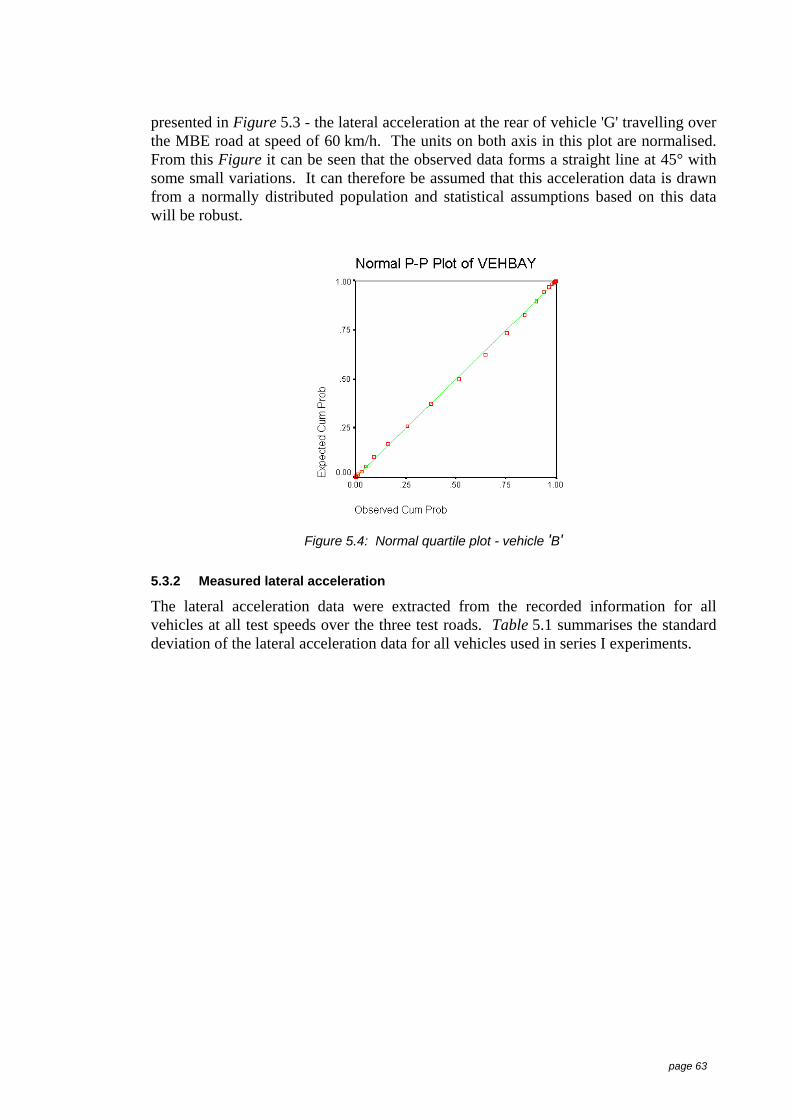
page 63
presented in Figure 5.3 - the lateral acceleration at the rear of vehicle 'G' travelling overthe MBE road at speed of 60 km/h. The units on both axis in this plot are normalised.From this Figure it can be seen that the observed data forms a straight line at 45° withsome small variations. It can therefore be assumed that this acceleration data is drawnfrom a normally distributed population and statistical assumptions based on this datawill be robust.
Figure 5.4: Normal quartile plot - vehicle 'B'
5.3.2 Measured lateral acceleration
The lateral acceleration data were extracted from the recorded information for allvehicles at all test speeds over the three test roads. Table 5.1 summarises the standarddeviation of the lateral acceleration data for all vehicles used in series I experiments.

page 64
Table 5.1: Measured lateral acceleration standard deviation
Standard Deviation Lateral Acceleration (g)Nominal test speed (km/h)
Vehicle Pavement 60 75 90Condition PM Trailer PM Trailer PM Trailer
A SAE 0.010 0.010 0.011 0.012 0.012 0.013MBE 0.007 0.005 0.008 0.004 0.005 0.002RCW 0.014 0.014 0.016 0.017 0.017 0.018
B SAE 0.010 0.012 0.011 0.016 0.013 0.018MBE 0.005 0.003 0.005 0.003 0.021 0.040RCW 0.014 0.018 0.015 0.024 0.018 0.027
C SAE 0.010 0.016 0.012 0.027 0.024 0.030MBE 0.005 0.003 0.021 0.052 0.027 0.065RCW 0.014 0.024 0.015 0.036 0.018 0.045
D SAE 0.010 0.010 0.012 0.011 0.006 0.001MBE 0.006 0.003 0.007 0.002 0.009 0.002RCW 0.015 0.015 0.016 0.014 0.019 0.019
E SAE 0.004 0.002 0.022 0.015 0.018 0.002MBE 0.006 0.003 0.027 0.031 0.044 0.037RCW 0.007 0.005 0.021 0.026 0.037 0.029
F SAE 0.036 0.018 0.041 0.027 0.040 0.027MBE 0.012 0.011 0.013 0.012 0.012 0.012RCW 0.030 0.034 0.033 0.042 0.036 0.045
Figure 5.5 is a plot of the standard deviation of the lateral acceleration at the rear trailerlongitudinal centre of gravity position against VSR for vehicle 'C'. Data acquired overall twelve test sections were used for this analysis. A strong positive linear relationshipwas identified between these two parameters. This analysis was conducted to force theintercept through the origin, ie. constant equals zero, a higher correlation could beachieved by not forcing through the origin but as the data was grouped away from theorigin it is assumed that the lateral acceleration would be zero for zero speed. The dataspread at the large VSR values indicates a non-linearity at the high speed and roughnessconditions.

page 65
0.00
0.02
0.04
0.06
0.08
40 60 80 100 120 140 160 180
VSR
SDLateral
Acceleration(g)
MeasuredRegression
Figure 5.5: Rear trailer lateral acceleration – vehicle 'C'
A similar strong relationship between the lateral acceleration at the rear trailer and VSRwas found for all vehicles used in the series I experiments.
As a strong relationship was shown between the lateral acceleration and VSR, it wasconsidered appropriate to investigate numerically processing of the lateral accelerationdata to estimate the lateral movement. The technique used to estimate vehicle lateralmovement will be discussed later in this Chapter.
5.4 Lateral movement from video imagesThe video-based information acquired during the series II field experiments wasprocessed to extract the relative lateral movement of the rear trailer from each videoframe. Calibration constants were then applied to this information to convert screen co-ordinates into engineering units - time in seconds and lateral movement in millimetres.A sample data file from processed video information is given in Appendix 7, Annex 4.
As with the other lateral movement and position data, summary statistics (mean,standard deviation, RMS, maximum and minimum, skewness and kurtosis) werecomputed for all video processed data. This information is shown in the top of thesample file in Appendix 7, Annex 4.
Figure 5.6 shows the video-based relative lateral movement of the rear of the A-doubletravelling over the MBE road at 75 km/h.
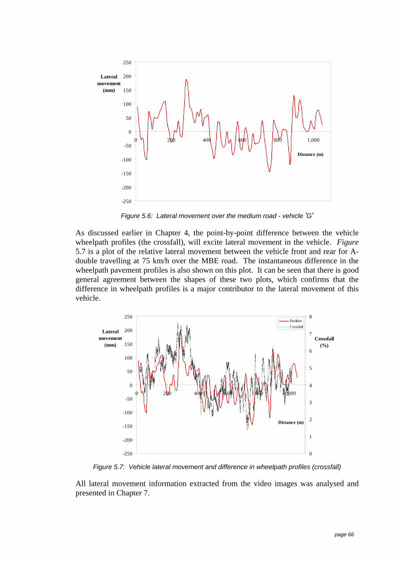
page 66
-250
-200
-150
-100
-50
0
50
100
150
200
250
0 200 400 600 800 1,000
Distance (m)
Lateralmovement
(mm)
Figure 5.6: Lateral movement over the medium road - vehicle 'G'
As discussed earlier in Chapter 4, the point-by-point difference between the vehiclewheelpath profiles (the crossfall), will excite lateral movement in the vehicle. Figure5.7 is a plot of the relative lateral movement between the vehicle front and rear for A-double travelling at 75 km/h over the MBE road. The instantaneous difference in thewheelpath pavement profiles is also shown on this plot. It can be seen that there is goodgeneral agreement between the shapes of these two plots, which confirms that thedifference in wheelpath profiles is a major contributor to the lateral movement of thisvehicle.
-250
-200
-150
-100
-50
0
50
100
150
200
250
0 200 400 600 800 1,000
Distance (m)
Lateralmovement
(mm)
0
1
2
3
4
5
6
7
8
Crossfall(%)
PositionCrossfall
Figure 5.7: Vehicle lateral movement and difference in wheelpath profiles (crossfall)
All lateral movement information extracted from the video images was analysed andpresented in Chapter 7.

page 67
5.5 Lateral movement estimates from lateral accelerationVehicle lateral movements were estimated from the recorded lateral acceleration,chassis height and the measured pavement wheelpath profiles. The lateral accelerationsignals were double integrated to estimate displacement, and the trailer roll angle wascomputed from the chassis height signals. The basis for this estimation is the numericintegration of the lateral acceleration (m/s/s) time series to give the velocity (m/s), andthe numeric integration of velocity to give displacement (m), as described by equation(1).
∫∫= )(ÿ)( tty (1)
The integration performs a numerical lowpass digital filter technique as outlined byBendat & Piersol (1971), using a recursive digital filter which acts like a lowpass filteras shown in equation (2):
)1()1( −+−= nnn ayxay (2)
where: a is exp⎭⎬⎫
⎩⎨⎧ ∆−
RCt
)1( −nay is the nth -1 lateral acceleration measured sample (m/s/s)For this application the form of equation (2) was applied as shown in equation (3):
)1(.. −+= nnn ydtayy α (3)
where: α (alpha) is the numeric integration feedback coefficient (is lessthan unity)
nay is the nth lateral acceleration measured sample (m/s/s)dt is the sampling interval (sec)n is the nth sampleyn is the estimated value.
This integration effectively estimates the area between each time sample, hence thesampling interval and the integration feedback coefficient are critical to the accuracy ofthis technique. A range of data sampling rates was used for the field experiments andthe values for the integration feedback coefficient were chosen iteratively for eachsampling rate. It was necessary to use values to 6 decimal places for the alpha value asshown in Table 5.2.
Table 5.2: Integration feedback coefficients
SamplingRate(sec)
Alpha
0.1 0.7900000.05 0.895990
0.033 0.9300000.025 0.9490000.01 0.979808
To confirm the iterative value and to predict a value for alpha, a linear regressionanalysis was conducted on the data in Table 5.3, using alpha as the dependent variableand the sampling rate as the independent variable.

page 68
Table 5.3: Coefficients to estimate integration feedback coefficient
Intercept Coefficient Correlationcoefficient
1.0009 -2.1086 0.9998
Table 5.3 lists the coefficients from the linear regression, a correlation coefficient of0.9998 was computed for this data, indicating that 99.98% of the variation in alpha isexplained by the sampling rate. This means that an accurate estimate of alpha can beobtained for any sampling rate within this range.
Trailer Roll Angle
During the field experiments accelerometers were attached to the trailer chassis, hencethe roll angle of the chassis influenced the measured trailer lateral acceleration byadding (or subtracting) a small component to the acceleration signal. The trailer rollangles were computed from the measured changes in trailer height (with reference to thepavement surface) of both the driver and passenger sides using equation (4):
Trn = ASIN ( )⎭⎬⎫
⎩⎨⎧
SpHdn-Hpn (4)
where: Hpn is rear trailer chassis height on the passenger side (m)Hdn is rear trailer chassis height on the driver side (m)Sp is Sensor spacing, constant (2.465 m)Tr is trailer roll angle (deg).
Pavement Crossfall
Similarly, to the trailer chassis roll angle, the crossfall of the pavement also influencedthe measured trailer lateral acceleration as it also adds (or subtracts) a small componentto the acceleration signal. This crossfall information was obtained from the WalkingProfiler measurements and the pavement surface angle was computed by equation (5):
Ran = ATAN ( )⎭⎬⎫
⎩⎨⎧
twn D -n P (5)
where: P n is the passenger side wheel path profile (m)D n is the driver side wheel path profile (m)tw is the trailer track width, constant (1.8 m)Ra is the pavement surface angle (deg).
Modified Lateral Acceleration
The trailer roll angle and pavement surface angles values were then applied to produce amodified lateral acceleration parameter, as shown in equation (6), which was used inequation (3) to estimate the lateral velocity. The lateral velocity was then integratedusing the form in equation (3) to produce lateral movement.

page 69
ay'n = {ay n + SIN(Tr n + Ra n)} - mean(ay') (6)
where: Tr n is the trailer roll angle (deg)Ra n is the equivalent pavement angle (deg)ay is the measured lateral acceleration (m/s/s)ay' is the corrected lateral acceleration (m/s/s).
The implementation of this technique was shown in George (1997) for this data set. Itshould be noted that the estimates from this method have a mean value of zero. This isbecause it is necessary to remove trends and offsets from the input data to prevent largedrifts in the numeric integration process.
The outputs from this method were compared with the video-based data from thesecond series of field experiments and subsequently applied to the measured data fromthe first test series.
5.6 Rearward amplificationRearward Amplification tests were conducted to provide performance information to beused for validating computer models, these tests were not a prime part of this study asthere has been many documented studies on this measure. These tests were performedon all vehicles in series I, and only vehicle 'G' in series II field experiments.Information from these tests was primarily used to validate computer models, the dataprocessing and outputs are reported below.
5.6.1 Background
Rearward Amplification is a prime measure of dynamic vehicle safety. It is theresponse of the trailers, in particular the rear trailer, to a rapid steer input manoeuvreand it describes the ability of the vehicle system to amplify the manoeuvre from thehauling unit to the last trailer. The rearward amplification phenomenon has beendocumented in many studies of multi-combination vehicle rollover accidents, such asErvin et al (1978), Fancher (1982), and Ervin and Guy (1986b). The level ofamplification is of concern as it reflects the vehicle's ability to sustain a rapidmanoeuvre without rolling over. Rearward amplification is defined as:
The ratio of the peak value of the lateral acceleration measured at the centre ofgravity of the rear most trailer to that at the centre of mass of the hauling unit in amanoeuvre causing the vehicle to move laterally into a path which is parallel to theinitial path.
Whilst the rearward amplification ratio is a useful measure to compare the dynamicstability of various vehicle types, it is a little difficult to determine or set an absolutelimit for a performance-based standard. This test, in its simplest form, is applying theamplification ratio to the maximum level of lateral acceleration at the hauling unit thatthe rear trailer can sustain without roll-over. For example if a vehicle has a rearwardamplification ratio of 2 and the rear trailer has a roll-limit of 0.3 g then the maximumlevel of lateral acceleration that the hauling unit can experience is 0.15 g without thetrailer rolling over.
The main use or interpretation of the rearward amplification ratio could be:

page 70
During a dynamic manoeuvre, does the vehicle remain upright (ie. not roll-over)and what is the maximum road space the vehicle occupies during the test?
Research has identified a number of elements that have first order sensitivities onrearward amplification. These elements, not necessarily in order of significanceinclude: the number of articulations, the wheelbase length of the trailers, the couplingtype ('A', 'B' or 'C' coupling), vehicle speed, steer input amplitude and frequency andaxle masses. Winkler et al (1992) developed a Lane Change test procedure for theSociety of Automotive Engineers (SAE) to evaluate rear amplification characteristicsfor combination vehicles. This procedure defines a set of parameters, test conditionsthat set the steering amplitude and frequency and hence make a controllable andreproducible test for comparative rearward amplification information. These controlparameters are:
• a path for the vehicle to follow
• a time period that the vehicle must pass between two fixed points (the testspeed)
For the first series of field experiments for this work the rearward amplification of eachvehicle configuration was obtained with a modified SAE test procedure. The lateraldisplacement for the steer path was reduced from 1.44 m in the SAE procedure to 1m.This was to ensure that the lateral displacement was not too severe and create a safetyproblem for the triple road-trains, as these experiments were conducted on public roadswithout traffic control. The effect of reducing the lateral displacement from 1.44 m to1 m reduced the lateral acceleration generated at the front unit from 0.15 g to 0.1 g. Itshould be noted that the frequency of the steer input has a primary influence on thevehicle response. The SAE test procedure defines the steer input frequency to be2.5 rad/sec (0.4Hz)
Figure 5.8: Driver view of the rearward amplification test course
Figure 5.8 shows the driver's view of the rearward amplification test course. Thiscourse was laid out to enable vehicles travelling from either direction to complete thetest. Hence the two lateral paths shown in the Figure. The vehicle shown in theforeground in Figure 5.8 was used to advise the driver of any on-coming traffic duringthe rearward amplification test. This course was on a new section of pavement near thesmooth test section for the trailing fidelity tests. The mean crossfall of pavement on thistest section was approximately 3%.

page 71
To reduce this risk of vehicle roll-over during the rearward amplification tests, outriggerwheels were attached to the rear of the rear trailer of each test vehicle. Figure 5.9shows the outrigger fitted to vehicle 'C'.
Figure 5.9: Outrigger attached to test vehicle 'C'
5.6.2 Series I - experiments
As outlined earlier the rearward amplification experiments were conducted with alateral displacement at the steer axle of 1m. Figure 5.10 shows a typical time history ofthe lateral acceleration at the longitudinal centre of gravity of the hauling unit and therear trailer. The maximum lateral acceleration recorded at the hauling unit ofapproximately 0.1g can be seen in this Figure, along with the acceleration amplificationand time lag of the trailer response.
-0.2
-0.1
0.0
0.1
0.2
0 1 2 3 4 5 6 7 8 9 10
Time (sec)
Lateral Acceleration
(g)
prime-mover
rear trailer
Figure 5.10: Typical rearward amplification time history - vehicle 'C'
Table 5.4 summarises the rearward amplification results. The mean of the measuredlateral accelerations at the hauling unit centre of gravity for the valid passes is presentedalong with the standard deviation. The rearward amplification ratio and standarddeviation are computed from the mean of the lateral acceleration at the rear trailer

page 72
divided by the mean value at the hauling unit. The dominant frequency of the lateralacceleration at the rear trailer was computed and presented for all valid passes.
Table 5.4: Rearward amplification results
Lateral Acceleration RearwardAmplification Frequency Valid
PassesVehicle (g) SD (ratio) SD (rad/s) SD
A 0.080 0.015 0.99 0.06 1.31 0.38 24B 0.069 0.011 1.34 0.15 1.56 0.42 11C 0.065 0.013 1.99 0.53 1.23 0.00 11D 0.108 0.012 1.07 0.09 1.76 0.61 8E 0.119 0.017 1.38 0.21 4.50 3.60 3
The results of rearward amplification tests are consistent with the notion that the valueof rearward amplification increases with the number of articulations in a combinationvehicle, (Ervin and Guy, 1986a); rearward amplification values of 0.99, 1.34 1.99 forthe single (vehicle 'A'), double (vehicle 'B'), and triple (vehicle 'C') articulated vehiclesrespectively.
It should be noted that these experiments were conducted with a reduced lateraldisplacement which produced a smaller lateral acceleration than that prescribed in theSAE test method. Ignoring the data for vehicle ‘E’ because of the small data size andthe high standard deviation of the steer input frequency, it can also be seen thatmeasured steer input frequency ranged from 1.2 to 1.8 rad/sec, which is well below theSAE define level of 2.5 rad/sec. It is acknowledged that the rearward amplification isinput frequency dependent therefore these results cannot be directly compared withresults from other tests.
There was insufficient valid data recorded for vehicle 'F' (the A-triple car carrier) toobtain meaningful results. During the rearward amplification experiments this vehiclewas driven in a conservative manner which did not provide valid data for rearwardamplification analysis. Figure 5.11 shows the lateral acceleration time history forvehicle 'F' undergoing a lane change test. The lack of sinusoidal shape in lateralacceleration at both the hauling unit and trailer response can be seen from this Figure.There are also high frequencies (approximately 6 rad/s) present in both the hauling unitand trailer lateral acceleration.

page 73
-0.3
-0.2
-0.1
0
0.1
0.2
0.3
0 2 4 6 8 10 12
time (sec)
Lateral Acceleration
(g)
PMTrailer
Figure 5.11: Typical lane change lateral acceleration time history for vehicle 'F'
5.6.3 Series II - experiments
During the series II field experiments rearward amplification tests were only conductedon the A-double vehicle (vehicle 'G'). These tests were conducted using the standardSAE test procedure, ie. with a lateral displacement of 1.44 m and target lateralacceleration of the hauling unit of 0.15 g. Figure 5.12 shows a typical time history ofthe lateral acceleration data. In particular the level of lateral acceleration of the haulingunit can be seen from this Figure to be approximately 0.15g as opposed to 0.1g for theseries I tests.
-0.2
-0.1
0.0
0.1
0.2
0.3
0 2 4 6 8 10 12 14
Time (sec)
Lateralacceleration
(g)rear trailer
prime-mover
Figure 5.12: Typical rearward amplification time history data - vehicle 'G'
The processed results from the rearward amplification tests for vehicle 'G' are presentedin Table 5.5. The variation of lateral acceleration between tests can be seen from thedata in this Table. For this data rearward amplification values were computed for bothpositive and negative maximum values. The difference between these rearwardamplification values are also shown in the Table. A rearward amplification of 1.5 is themean of all values.

page 74
Table 5.5: Vehicle 'G' rearward amplification results
Lateral accelerationHauling unit Rear trailer RA Speed
Run Max Min Max Min Max Min (km/h)1 0.12 -0.09 0.17 -0.12 1.42 1.32 752 0.14 -0.12 0.21 -0.14 1.51 1.20 883 0.13 -0.11 0.23 -0.15 1.74 1.37 924 0.09 -0.08 0.13 -0.11 1.49 1.32 895 0.10 -0.10 0.17 -0.14 1.60 1.38 89
Mean 1.58 1.32 89.5SD 0.12 0.08 1.8

page 75
5.7 SummaryA data processing technique to extract the vehicle lateral position from the recorded LPIdata was developed and trialled. This processing was then applied to all recorded LPIdata from vehicles 'A', 'B' and 'C'. As shown in the preliminary analysis in the previousChapter, no linear relationships were found between the lateral position information andthe control variables. Nevertheless subsequent processing was conducted on therecorded lateral acceleration and trailer chassis height data to estimate the vehiclelateral movement.
Purpose built video-based instrumentation was used to collect relative (front to rear)lateral movement information. Vehicle lateral movement information was successfullyextracted and processed from the video images. This information was used asfundamental data to provide an understanding of vehicle lateral performance and as areference to compare predicted and estimated information from various sources. Thisanalysis and subsequent supplementary data from computer simulations are presented inChapter 7.
A technique to estimate the lateral movement from the recorded lateral acceleration andthe trailer roll angle was described. The application of this technique to the datarecorded on the test vehicles is shown in Chapter 7.
The validation of computer models using rearward amplification data recorded duringseries II experiments, and computer simulation using the processed video-based lateralmovement information will be discussed in the following Chapter.

page 76
6 Computer simulation
6.1 IntroductionAs identified by the project workshop reported in Chapter 2, the ability to predict theperformance of a range of vehicles is essential for a performance-based route selectionsystem. The outputs from this research were used to validate computer models andlateral movement simulations.
Computer modelling and the development of the capability to simulate the lateralbehaviour of heavy vehicles were conducted at ARRB TR from mid 1995 to January1999. Initial modelling and simulations were conducted on the vehicles used for bothseries I and II tests. Some difficulties were encountered in validating the simulationoutputs against the measured data and ultimately a second modelling software packagewas used to develop vehicle models and produce simulations.
6.2 Computer modelsInitially the development of a computer simulation model was undertaken as part of thiswork. This model was developed using the BAMMS (Bondgraph-based Algorithm forModelling Multibody) modelling package which was developed at the Delft Universityof Technology, Verheul et al (1994). One of the features of BAMMS is to provide aflexible user extendable software tool for the development and analysis of continuoussimulation models. The Bondgraph method defines the relationship of a mechanicalsystem by means of a graphical representation of the power flow in the system. Thephysical relations of the system are represented as components connected by powerbonds. BAMMS treats the modelling and simulation as two separate programs. Theuser creates the modelling component from predefined sub-models, which are storedand accessed as ASCII formatted macros.
The BAMMS modelling software was used to model the vehicles used for both testseries. Some difficulties were encountered when validating the simulation outputsagainst the measured data and ultimately this modelling package was abandoned andADAMS (Automatic Dynamic Analysis of Mechanical Systems) modelling softwarewas used to develop vehicle models and produce simulations.
For the sake of completeness, some outputs from both the BAMMS and the initialADAMS simulations are presented in this Chapter.
6.3 BAMMSSome outputs from the BAMMS simulations are presented in the following Figures forthe two vehicles used in the series II experiments. Figure 6.1 shows the simulationoutputs for the three test speeds over the three pavement conditions. As shown in thisFigure there is general agreement between the measured and simulated values for thestandard deviation of the lateral acceleration at the rear of the last trailer.
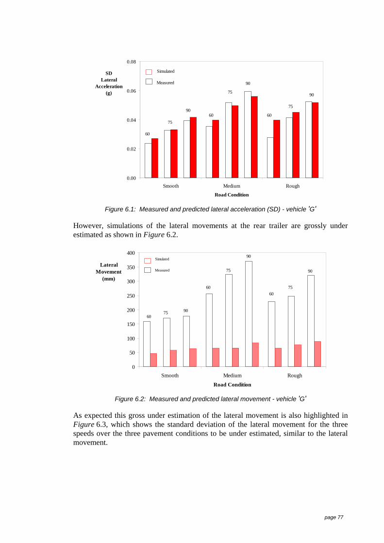
page 77
0.00
0.02
0.04
0.06
0.08
Smooth Medium Rough
Road Condition
SDLateral
Acceleration(g)
756060
60
75
75
90
90
90
Simulated
Measured
Figure 6.1: Measured and predicted lateral acceleration (SD) - vehicle 'G'
However, simulations of the lateral movements at the rear trailer are grossly underestimated as shown in Figure 6.2.
0
50
100
150
200
250
300
350
400
Smooth Medium Rough
Road Condition
LateralMovement
(mm)
75
6060
60
75
75
90
90
90
Simulated
Measured
Figure 6.2: Measured and predicted lateral movement - vehicle 'G'
As expected this gross under estimation of the lateral movement is also highlighted inFigure 6.3, which shows the standard deviation of the lateral movement for the threespeeds over the three pavement conditions to be under estimated, similar to the lateralmovement.

page 78
0
10
20
30
40
50
60
70
80
Smooth Medium Rough
Road Condition
SDLateral
Movement(mm)
75
60
60
60
75
75
90
90
90Simulated
Measured
Figure 6.3: Measured and predicted lateral movement (SD) - vehicle 'G'
Similar gross under estimations of the lateral movement for the truck-trailer (vehicle'H') were also produced by BAMMS. These are shown in Figure 6.4 for four testspeeds over the three pavement conditions.
0
100
200
300
400
500
Smooth Medium Rough
Road Condition
LateralMovement
(mm)
75
6060
60
75
75
90
90
90
100100
100
Simulated
Measured
Figure 6.4: Measured and predicted lateral movement - vehicle 'H'
6.4 Moving from BAMMSAs a consequence of the poor results from BAMMS (despite concerted efforts toimprove its performance including engaging the developer from the Netherlands) it wasdecided to abandon BAMMS and seek another heavy vehicle modelling and simulationpackage.
ADAMS software was used to model vehicle 'G' and the rearward amplificationinformation obtained from the field experiments was used to validate the modelling.

page 79
Vehicle lateral movement information extracted from the video-based instrumentationwas used to validate the ADAMS simulations.
ADAMS was developed at the University of Michigan in the 1970’s. It was enhancedand further developed into a commercial product by Mechanical Dynamics Inc.ADAMS locates and orientates all the parts of the mechanical system under analysisand fully describes them in terms of six co-ordinates: three translational and threeangular. The time dependent translational and angular displacements, velocities, andaccelerations are stored in the state vectors, which provide a complete description of themechanical system for a multi-body system analysis. This software has been usedextensively throughout the automotive industry in a number of applications such as thedesign and development of suspension systems and the ride and handling characteristicsof both passenger and heavy vehicles.
Computer models were created in ADAMS for a range of common vehicle types and thelateral movement of these vehicle models was estimated using measured pavementprofiles as an input to the simulation process. The validation of vehicle models and thepredictive ability of these modelling systems will be discussed later.
6.5 Validating ADAMS modelsA program was undertaken at ARRB TR to develop computer models using ADAMS.Whilst computer modelling was not part of this thesis, the data acquired during therearward amplification tests was used to validate computer model outputs, Elischer &Prem (1997). Figure 6.5 shows the lateral acceleration at the prime mover for five fieldrearward amplification tests and the simulated results from ADAMS.
-0.20
-0.15
-0.10
-0.05
0.00
0.05
0.10
0.15
0.20
3 4 5 6 7 8 9 10
Time (s)
LateralAcceleration
(g)
Run 1Run 2Run 3Run 4Run 5Simulated
source: Elischer and Prem (1997)
Figure 6.5: Simulated and measured hauling unit lateral accelerations - vehicle 'G'
Figure 6.6 shows the measured and predicted lateral acceleration at the rear trailer ofvehicle 'G' during the rearward amplification test. It can be seen from both Figures 6.5and 6.6 that the time histories of the simulated lateral accelerations are a goodrepresentation of both the shape and amplitude of the measured data.
Elischer & Prem concluded from their validation study that:

page 80
"The validation results in the time domain are very good using the adopted modeland associated parameters. Quantifying errors between the simulated responsesand the full-scale responses is very difficult due to the variation in full-scale datathat inevitably occurs. However, there is a 6% error between the simulatedrearward amplification and the average rearward amplification of the five 88 km/hfull-scale tests.
ADAMS is capable of producing realistic simulations and results of transientvehicle dynamics, though it is stressed that a suitable amount of data is required".
-0.20
-0.10
0.00
0.10
0.20
0.30
3 4 5 6 7 8 9 10Time (s)
LateralAcceleration
(g)
Run 1Run 2Run 3Run 4Run 5Simulated
source: Elischer and Prem (1997)
Figure 6.6: Simulated and measured rear trailer lateral acceleration - vehicle 'G'
Figure 6.7 shows a clear plot of the simulated lateral acceleration at the hauling unit andrear trailer for the rearward amplification test for vehicle 'G'.
-0.2
-0.1
0.0
0.1
0.2
0.3
3 4 5 6 7 8 9 10
Time (s)
LateralAcceleration
(g)
prime-mover
rear trailer
source: Elischer and Prem (1997)
Figure 6.7: Simulated lateral acceleration for a rearward amplification test - vehicle 'G'
6.6 Validating ADAMS simulationsLateral movement simulations were conducted for vehicle 'G' using a computer modelthat was validated against the rearward amplification measurements. To confirm the

page 81
simulation predicative accuracy the outputs from computer simulations were comparedwith the video-based lateral movement measurements. These data were mean zeroedand are presented in Figure 6.8 where it can seen that the ADAMS simulation providesa good representation of both the amplitude and shape of the video-based data.However, it can also be seen from this Figure that there is a 'certain' amount ofvariability in the video-based measurements.
The variability in the video-based (and most field) measurements could be contributedto a number of sources, such as:
• The variation in the vehicle speed during the measurement;
• The variation in vehicle path during the measurement (ie. the lateral positioningof the vehicle);
• Difference in steering activity;
• The error in translating the lateral information from the video recording to realcoordinates;
• General measurement errors, such as electrical noise, transducer accuracy,linearity and repeatability.
-300
-200
-100
0
100
200
300
0 100 200 300 400 500 600 700 800 900 1,000
Distance (m)
LateralMovement
(mm)
SimulatedVideo 1Video 2Video 3
Figure 6.8: Predicted lateral movement and video-based measurements - vehicle 'G'
As described in Chapter 5 lateral movement estimates were processed using measuredlateral acceleration and chassis height data. Comparisons between measured (video-based), simulated and estimated (acceleration-based) lateral movement informationwere conducted. Table 6.1 summarises the lateral movements for vehicle 'G' travellingover MBE at 90 km/h from three sources; simulated, estimated from the lateralacceleration, and the video-based measurements.

page 82
Table 6.1: Comparison between the measured, estimated and simulated lateralmovements
Lateral Movement (mm)SD Range
Video 1 71 394Video 2 80 376Video 3 70 341
Mean 74 371Simulation 83 447Estimated 78 453
The variability in the video-based measurements is also shown in Table 6.1.Nevertheless, the difference in the total movement between the three video-basedsamples is 53 mm with less than 9 mm difference in the standard deviations. Thesimulated movement is 21% larger than the mean of the 3 video-based measurements(371). Similarly, the estimated movement from the lateral acceleration is 22% largerthan the mean of the video-based measurements.
It should be noted that the simulations are predictions of the absolute movement of therear of the vehicle, in contrast with the video-based measurements which show thedifference in lateral movements between the front and rear of the vehicle.
6.6.1 Comparing three lateral movement data sources
It is of interest to examine the relationships between the three methods of obtainingvehicle lateral movement. Figure 6.9 shows the time histories of these three measuresfor vehicle 'G' travelling over the medium road at 90 km/h. Similar to Figure 6.8, it canbe seen from Figure 6.9 that there is a good representation of both the amplitude andshape between these measurements.
-250
-200
-150
-100
-50
0
50
100
150
200
250
300
0 5 10 15 20 25 30 35 40
Time (s)
LateralMovement
(mm)
Acceleration basedVideo basedSimulated
Figure 6.9: Three methods of obtaining lateral movement - vehicle 'G'
To further examine the validity of the simulation outputs a spectral analysis wasconducted on the video-based and the simulated lateral movements.

page 83
The purpose of this analysis was to examine the dominant frequencies of lateral activityfor vehicle 'G' travelling over MBE at 90 km/h from these data sets.
The spectral analysis produced PSD plots as shown in Figure 6.10. It can be seen fromthis analysis that the dominant frequency for the lateral movements from the video-based data are all around 0.45 Hz, and approximately 0.3 Hz for the simulated lateralmovement.
0.00
0.02
0.04
0.06
0.08
0.0 0.2 0.4 0.6 0.8 1.0 1.2 1.4 1.6 1.8 2.0
Frequency (Hz)
PSD(m^2/Hz)
SimulationVideo 1Video 2Video 3
Figure 6.10: PSD of lateral movement for vehicle 'G'
In addition to spectral analysis, an analysis to determine the coherence between thesimulated lateral movement and three video-based measurements was conducted.
In a frequency domain analysis the coherence is the ratio of the square of the crossspectral density function to the product of the spectral density function for the two timeseries data. The coherence can take a value from 0 to 1, and a linear system with nonoise will have a maximum value of unity at all frequencies. A coherence analysis isprincipally used when determining the transfer function (the input versus outputrelationship) of an electrical or mechanical system, such as when studying seatingdynamics. Possible causes for low coherence outlined by Griffin (1990) are:
• Non-linear relationship between the two data sets;
• Noise in one of the data sets;
• Rapid change in magnitude of the input or output spectrum with frequency.
The outputs from this analysis are presented in Figure 6.11 where it can be seen that thehighest coherence between the simulated and measured data is around 0.96 at 0.7 Hz. Asmall peak at this frequency can be seen on the PSD plot (Figure 6.10), however, thereis less coherence at the dominant frequencies of 0.3 and 0.45 Hz. It can therefore beconcluded from this analysis that there is not a strong linear relationship between thevideo-based and the simulated lateral movements. The apparent coherence at 0.96 and0.7 Hz could be attributed to noise.
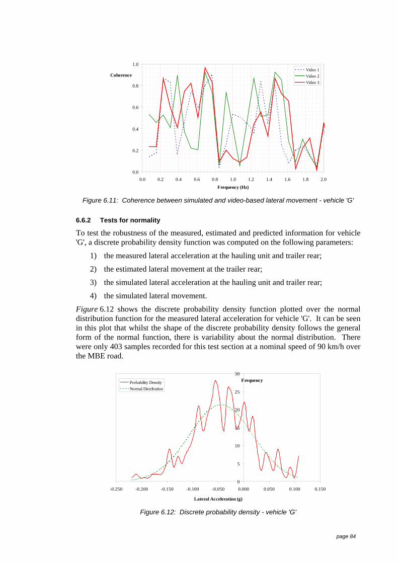
page 84
0.0
0.2
0.4
0.6
0.8
1.0
0.0 0.2 0.4 0.6 0.8 1.0 1.2 1.4 1.6 1.8 2.0
Frequency (Hz)
CoherenceVideo 1Video 2Video 3
Figure 6.11: Coherence between simulated and video-based lateral movement - vehicle 'G'
6.6.2 Tests for normality
To test the robustness of the measured, estimated and predicted information for vehicle'G', a discrete probability density function was computed on the following parameters:
1) the measured lateral acceleration at the hauling unit and trailer rear;
2) the estimated lateral movement at the trailer rear;
3) the simulated lateral acceleration at the hauling unit and trailer rear;
4) the simulated lateral movement.
Figure 6.12 shows the discrete probability density function plotted over the normaldistribution function for the measured lateral acceleration for vehicle 'G'. It can be seenin this plot that whilst the shape of the discrete probability density follows the generalform of the normal function, there is variability about the normal distribution. Therewere only 403 samples recorded for this test section at a nominal speed of 90 km/h overthe MBE road.
0
5
10
15
20
25
30
-0.250 -0.200 -0.150 -0.100 -0.050 0.000 0.050 0.100 0.150
Lateral Acceleration (g)
FrequencyProbability DensityNormal Distribution
Figure 6.12: Discrete probability density - vehicle 'G'

page 85
To further assess the normality of this data a normal quartile plot was conducted andthis is presented in Figure 6.13. It can be seen from Figure that the majority of the datalies over the 45° line confirming that the lateral acceleration measured at the rear ofvehicle 'G' over MBE was drawn from a normally distributed population.
Normal Q-Q Plot of VEHGAY
Observed Value
.2.1-.0-.1-.2-.3
Expe
cted
Nor
mal
Val
ue
.2
.1
-.0
-.1
-.2
-.3
Figure 6.13: Normal quartile plot - vehicle 'G'
To determine the reliability and robustness of statistical assumptions using the lateralacceleration a discrete probability density function was computed on both the simulatedlateral acceleration and movement data.
It can be seen in Figure 6.14 that the simulated lateral movement for the A-doubletravelling at 90 km/h over MBE is approximately normally distributed. However, thereappears to be more spread than the measured lateral acceleration data as shown inFigure 6.12. This could be due to the higher sampling rate in the measured lateralacceleration.
0
5
10
15
20
25
30
-0.3 -0.2 -0.1 0.0 0.1 0.2 0.3
Lateral Acceleration (g)
Frequency
Figure 6.14: Predicted lateral acceleration discrete probability density - A-double
Figure 6.15 shows the normal quartile plot for the predicted lateral acceleration, andfrom this plot it can be concluded that the predicted lateral acceleration data at the rearof vehicle 'G' appears to be drawn from a normally distributed sample.

page 86
Normal Q-Q Plot of VEHGPY
Observed Value
2001000-100-200-300-400-500-600
Expe
cted
Nor
mal
Val
ue
200
100
0
-100
-200
-300
-400
-500
-600
Figure 6.15: Predicted lateral acceleration normal quartile - A-double
As with the predicted lateral acceleration, a discrete probability density was computedfor the predicted lateral movement of the A-double travelling over MBE at 90 km/h, andplotted over the normal distribution function, Figure 6.16
0
5
10
15
20
25
-600 -500 -400 -300 -200 -100 0 100 200
Lateral Movement (mm)
Frequency
Figure 6.16: Predicted lateral movement discrete probability density - A-double
It can be seen from Figure 6.16 that the lateral movement at the rear trailer isapproximately normally distributed, however, to confirm the normality of this data anormal quartile plot was conducted as shown in Figure 6.17.

page 87
Normal Q-Q Plot of VEHGPAY
Observed Value
.3.2.1-.0-.1-.2-.3
Expe
cted
Nor
mal
Val
ue
.3
.2
.1
-.0
-.1
-.2
-.3
Figure 6.17: Predicted lateral movement normal quartile - A-double
The predicted lateral movement normal quartile plot in Figure 6.17 shows lessnormality that the lateral acceleration in Figure 6.13, however, it is considered that withthe relatively small variations from the normal line that the predicted lateral movementdata is drawn from a normal population.
It can therefore be concluded from this analysis that the simulated and estimated lateralmovement appear to be normally distributed which indicates that valid statisticalassumptions can be made for these data sets.
6.7 Simulating lateral behaviorComputer models were created for a range of common vehicle types. The values andassumption for the modelling parameters are given in Elischer & Prem (1997). Thedimensions for these vehicles were taken from Austroads (1995) which gives the 85th
percentile dimensions of vehicles in the Australian fleet. The dimensions for thevehicles not covered in the Austroads publication (truck-trailers, 19 m B-double, B-triple and rigid-plus-three) were based on typical vehicles in the fleet.
All vehicles, except for the truck-trailers, were loaded to the legal axle mass limits andthe maximum height limit (4.3 m). Loading the vehicles to these limits with ahomogeneous load produced a load centre-of-gravity height of approximately 2.9m. Asa comparison, the estimated load centre-of-gravity height for vehicles loaded withpallets of bricks, (test vehicles 'A', 'B' and 'C') was approximately 1.8 m. This higherload centre-of-gravity height should produce 'worst-case' simulation outputs. Thisdifference along with other parameters may account for any difference betweenmeasured and simulated data. The axle loads on the truck-trailer simulated vehicleswere set to preserve the legal truck-trailer mass ratios. These truck-trailer mass ratiosare 1:1 for a 3 axle truck towing a 3 axle trailer (R12-T12), and 1:1.22 for a 3 axle trucktowing a 4 axle trailer (R12-T22), as outlined by the following; NRTC (1997),Victorian Government (1999) and Queensland Transport (1998).
Table 6.2 lists the vehicle types that were modelled for computer simulations. ThisTable contains vehicle codes, lengths and GCMs. Their dimensions and axle massesare given in Appendix 15.
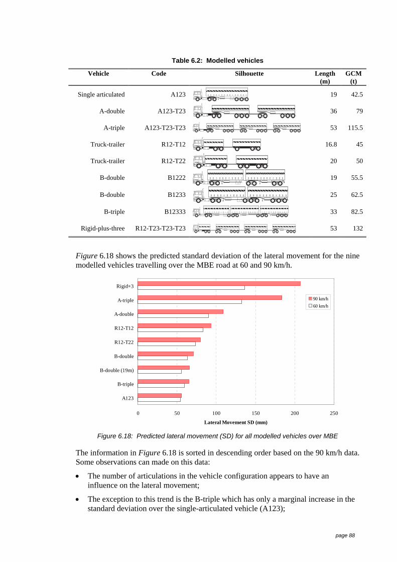
page 88
Table 6.2: Modelled vehicles
Vehicle Code Silhouette Length(m)
GCM(t)
Single articulated A123 19 42.5
A-double A123-T23 36 79
A-triple A123-T23-T23 53 115.5
Truck-trailer R12-T12 16.8 45
Truck-trailer R12-T22 20 50
B-double B1222 19 55.5
B-double B1233 25 62.5
B-triple B12333 33 82.5
Rigid-plus-three R12-T23-T23-T23 53 132
Figure 6.18 shows the predicted standard deviation of the lateral movement for the ninemodelled vehicles travelling over the MBE road at 60 and 90 km/h.
0 50 100 150 200 250
A123
B-triple
B-double (19m)
B-double
R12-T22
R12-T12
A-double
A-triple
Rigid+3
Lateral Movement SD (mm)
90 km/h60 km/h
Figure 6.18: Predicted lateral movement (SD) for all modelled vehicles over MBE
The information in Figure 6.18 is sorted in descending order based on the 90 km/h data.Some observations can made on this data:
• The number of articulations in the vehicle configuration appears to have aninfluence on the lateral movement;
• The exception to this trend is the B-triple which has only a marginal increase in thestandard deviation over the single-articulated vehicle (A123);
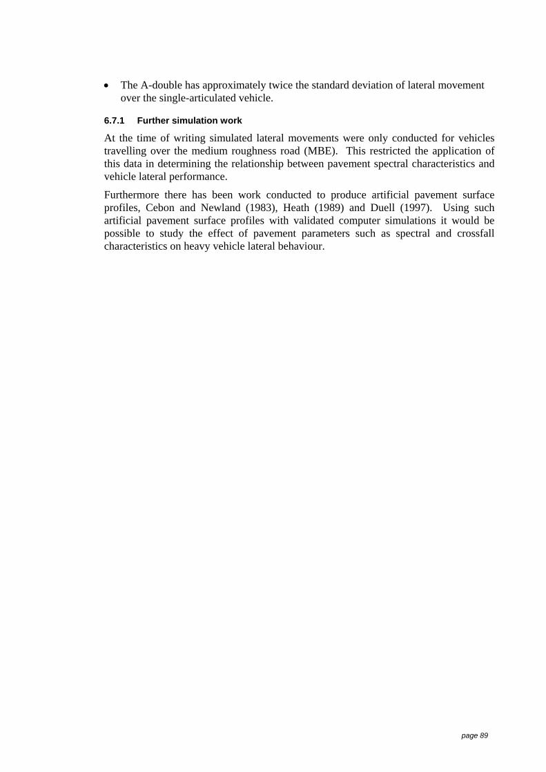
page 89
• The A-double has approximately twice the standard deviation of lateral movementover the single-articulated vehicle.
6.7.1 Further simulation work
At the time of writing simulated lateral movements were only conducted for vehiclestravelling over the medium roughness road (MBE). This restricted the application ofthis data in determining the relationship between pavement spectral characteristics andvehicle lateral performance.
Furthermore there has been work conducted to produce artificial pavement surfaceprofiles, Cebon and Newland (1983), Heath (1989) and Duell (1997). Using suchartificial pavement surface profiles with validated computer simulations it would bepossible to study the effect of pavement parameters such as spectral and crossfallcharacteristics on heavy vehicle lateral behaviour.

page 90
6.8 SummaryVehicle simulations produced by the BAMMS software predicted the lateralaccelerations with an acceptable level of accuracy, however, the predictions of thevehicle lateral movement were grossly under-estimated and use of this software wasdiscontinued.
The ADAMS modelling and simulation package was validated using measuredrearward amplification and video-based lateral movement data from this work.ADAMS predicted lateral movement (standard deviation) 20% larger than the video-based measurements. There was also a difference between the dominant frequencies ofthe video-based lateral movement and the predictions, 0.45 Hz and 0.3 Hz respectively.It was also shown that there was not high coherence between simulated lateralmovement of the rear trailer and the three repeat video-based measurements.
However, it was shown that the simulated lateral acceleration and lateral movementdata were approximately normally distributed.
Relatively high mean values were produced from the simulated lateral movement. Itwas not possible to validate the vehicle lateral position in the lane from this field data -the video-based measurements were the relative movement between the hauling unitand the last trailer, and the lateral movement estimates derived from the measuredlateral acceleration were mean zeroed to reduce cumulative errors during the integrationprocess.
A spectral analysis showed that there was low coherence between the lateral movementat the last trailer and the spectral characteristics of the pavement.
Nine common vehicle types were modelled and their lateral movements were simulatedover the MBE road. The information from the computer simulations providedsupplementary data to the measured data in this work, and the following Chaptercontains the analysis of this data.

page 91
7 Data Analysis
7.1 IntroductionThe previous Chapters described the field experiments, data processing, and the use ofthe field data to validate computer models and simulated lateral movement. ThisChapter describes the analysis of these data sets.
7.2 Lateral movement from video imagesThe video-based data were processed and analysed and the lateral movements weredetermined for both test vehicles from the series II field experiments. These lateralmovements are summarised in Table 7.1 for the A-double (vehicle 'G') and in Table 7.7for the truck-trailer (vehicle 'H'). These data are presented as peak to peak valueslabelled as total movement averaged over a number of valid repeat passes and thestandard deviation (SD) is the mean of the standard deviations of the lateral movementof the valid passes.
7.2.1 Vehicle 'G'
The data in Table 7.1 lists the total lateral movement and the standard deviation of therear trailer relative to the hauling unit for vehicle 'G' as it travelled over the three testroads at the three nominated speeds. This information shows that the rear of the trailerhas moved laterally within a total range of approximately 370 mm with reference to thehauling unit when travelling over the MBE road at 90 km/h. This information will bediscussed in relation to the road space requirements later in this Chapter.
Table 7.1: Video-based lateral movement - vehicle 'G'
Relative lateral movement (mm)Nominal vehicle speed (km/h)
60 75 90Total SD Total SD Total SD
Smooth 159 29 170 32 178 39
Medium 256 50 323 63 371 73
Rough 229 45 321 50 321 71
The data to construct the information in Table 7.1 is presented the Tables 7.2, 7.3 and7.4 following. The column labels in these Tables are defined as follows:Mean - the computed average value of the relative lateral movementSD - the computed standard deviation value of the relative lateral movementMax - the maximum value of the relative lateral movementMin - the minimum value of the relative lateral movementRange - the absolute sum of the maximum and minimum valuesSpeed - the measured average speed of the vehicle over the test section

page 92
Table 7.2: Video-based lateral movement SAE summary - vehicle 'G'
Relative lateral movement (mm) SpeedMean SD Max Min Range (km/h)
Run 1 4.3 29.1 77.6 -72.1 150 60.3Run 2 -0.6 28.5 85.5 -82.9 168 61.0Mean 1.8 28.8 81.5 -77.5 159 60.7
Run 1 -1.0 31.9 96.4 -90.6 187 75.3Run 2 0.2 32.3 77.1 -76.8 154 75.9Mean -0.4 32.1 86.7 -83.7 170 75.6
Run 1 -3.5 41.6 118.3 -84.1 202 91.7Run 2 10.5 34.3 77.5 -73.0 151 91.4Run 3 16.7 40.0 95.9 -84.6 180 91.1Mean 7.9 38.6 97.3 -80.5 178 91.4
Table 7.3: Video-based lateral movement MBE summary - vehicle 'G'
Relative lateral movement (mm) SpeedMean SD Max Min Range (km/h)
Run 1 15.1 49.9 156.7 -102.4 259 60.8Run 2 4.5 50.2 134.3 -119.3 254 61.5Mean 10 50 146 -111 256 61
Run 1 8.4 62.4 186.4 -144.7 331 75.5Run 2 -0.7 63.9 177.9 -137.7 316 75.1Mean 4 63 182 -141 323 75
Run 1 15.9 70.8 234.6 -159.7 394 90.6Run 2 35.9 79.2 227.2 -148.7 376 91.2Run 3 17.5 70.4 197.4 -143.9 341 89.4Mean 23 73 220 -151 371 90

page 93
Table 7.4: Video-based lateral movement RCW summary - vehicle 'G'
Relative lateral movement (mm) SpeedMean SD Max Min Range (km/h)
Run 1 36.1 49.2 183 -64.3 247 58.9Run 2 45.0 47.4 182 -57.8 240 59.3Run 3 43.8 37.6 175 -24.6 199 60.0Mean 41.6 44.7 180 -48.9 229 59.4
Run 1 27.0 42.7 153 -63.7 217 72.8Run 2 38.3 51.6 182 -61.5 244 73.0Run 3 36.8 55.4 201 -83.4 285 74.3Mean 34.0 49.9 179 -69.5 248 73.4
Run 1 38.3 66.8 164 -109.5 273 88.2Run 2 42.0 74.7 224 -144.6 368 91.2Mean 40.1 70.8 194 -127.1 321 89.7
For the A-double (vehicle 'G'), the relationship between the lateral movement, speedand pavement condition is shown in Figure 7.1.
0
100
200
300
400
500
SAE SAW MBE MBW RCE RCW
Road Condition
Lateralmovement
(mm)
60 km/h75 km/h90 km/h
Figure 7.1: Measured relative lateral movement - vehicle 'G'
It can be seen that there is an equal or greater lateral movement over the medium road(MBE) compared with the rough road (RCW). Whilst further information is required toexplore this apparent anomaly, possible causes or areas that could contribute to this arethe pavement surface spectral characteristics, difference in wheel path profiles, thepavement crossfall or the pavement roughness of the MBE test road. The apparentdifference in the pavement wheelpath roughnesses were highlighted in Table 4.4.
7.2.1.1 Significance of independent variables
The significance of the VSR (pavement condition and vehicle speed) on the level oflateral movement at the rear trailer was examined using an Analysis of Variance(ANOVA). ANOVA is based on the concept of variance and it identifies the sources of

page 94
variation in the data to assess the relative importance of each parameter. Due to thestructure of the data, a multiple-regression analysis (MLR) was the easiest way ofproducing an ANOVA table.
Table 7.5 summarises the regression statistics from the MLR analysis, and shows that78% of the observed variation in the lateral movement for vehicle 'G' is explained bythe VSR.
Table 7.5: Regression statistics - vehicle 'G'
Multiple R 0.89R Square 0.78
Adjusted R Square 0.77Standard Error 38.18Observations 18
The ANOVA output in Table 7.6 shows that the regression coefficient (VSR) is notequal to zero, F(1,16)=58, p<0.001, and that it is a very significant predictor of lateralmovement for vehicle 'G' with p<0.001. It should be noted that for an ANOVA analysisit is important that there are not high correlations between the independent variables(co-variables). Therefore conducting an ANOVA with VSR, pavement condition andvehicle speed as independent variables would not produce meaningful results as there ishigh correlation between these variables.
Table 7.6: ANOVA Output - vehicle 'G'
df SS MS F Sign FRegression 1 84882 84882 58 0.00000Residual 16 23327 1458
Total 17 108208
Coefficients Standard Error t Stat P-valueIntercept -48.35 39.05 -1.238 0.2335
VSR 2.42 0.32 7.630 0.0000
7.2.2 Vehicle 'H'
The video-based lateral movement data for vehicle 'H' is given in Table 7.7. It can beseen from this data that the rear of this trailer has moved laterally a total of 278 mmwith reference to the prime mover while travelling over the medium roughnesspavement at 90 km/h. This information will be discussed as the road spacerequirements later in this Chapter.

page 95
Table 7.7: Video-based lateral movement – vehicle 'H'
Relative lateral movement (mm)Speed (km/h)
60 75 90 100Total SD Total SD Total SD Total SD
Smooth 124 21 138 24 165 30 163 32
Medium 197 35 200 42 278 48 261 46
Rough 183 28 214 37 241 47 271 52
Figure 7.2 shows the effect of vehicle speed and pavement type on the lateral behaviourof the truck-trailer. A similar lateral response was measured for this vehicle to the A-double - an equal or greater lateral movement over the medium road (MBE) comparedwith the rough road (RCW). It is of interest to note the effect of vehicle speed over theMBE test section - a greater lateral movement at a test speed of 90 km/h than at100 km/h. This may indicate a 'tuning' of the vehicle wheelbase to the pavementwavelength characteristics which would be exciting a different response. This tuning isknown as 'wheel-base filtering', and is described by Gillespie (1985):
"as a vehicle traverses a road, the roughness excitation at the different axles is notindependent. The rear wheels see nearly the same input profile as the front wheels,only delayed in time. The time delay is equal to the wheelbase divided by the speedof travel. The time delay acts to filter the bounce and pitch excitation amplitude".
0
100
200
300
400
500
SAE SAW MBE MBW RCE RCW
Road Condition
Lateralmovement
(mm)
60 km/h75 km/h90 km/h100 km/h
Figure 7.2: Measured relative lateral movement - vehicle 'H'
7.2.2.1 Significance of independent variables
Similar to vehicle 'G' an ANOVA analysis was conducted on the data for vehicle 'H' todetermine the significance of the VSR on the lateral movement at the rear of vehicle 'H'.
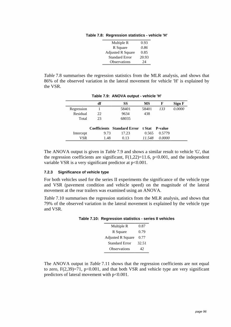
page 96
Table 7.8: Regression statistics - vehicle 'H'
Multiple R 0.93R Square 0.86
Adjusted R Square 0.85Standard Error 20.93Observations 24
Table 7.8 summarises the regression statistics from the MLR analysis, and shows that86% of the observed variation in the lateral movement for vehicle 'H' is explained bythe VSR.
Table 7.9: ANOVA output - vehicle 'H'
df SS MS F Sign FRegression 1 58401 58401 133 0.0000
Residual 22 9634 438Total 23 68035
Coefficients Standard Error t Stat P-valueIntercept 9.73 17.23 0.565 0.5779
VSR 1.48 0.13 11.548 0.0000
The ANOVA output is given in Table 7.9 and shows a similar result to vehicle 'G', thatthe regression coefficients are significant, F(1,22)=11.6, p<0.001, and the independentvariable VSR is a very significant predictor at p<0.001.
7.2.3 Significance of vehicle type
For both vehicles used for the series II experiments the significance of the vehicle typeand VSR (pavement condition and vehicle speed) on the magnitude of the lateralmovement at the rear trailers was examined using an ANOVA.
Table 7.10 summarises the regression statistics from the MLR analysis, and shows that79% of the observed variation in the lateral movement is explained by the vehicle typeand VSR.
Table 7.10: Regression statistics - series II vehicles
Multiple R 0.87R Square 0.79
Adjusted R Square 0.77Standard Error 32.51Observations 42
The ANOVA output in Table 7.11 shows that the regression coefficients are not equalto zero, F(2,39)=71, p<0.001, and that both VSR and vehicle type are very significantpredictors of lateral movement with p<0.001.

page 97
Table 7.11: ANOVA output - series II vehicles
df SS MS F Sign FRegression 2 150729 75365 71 0.0000Residual 39 41223 1057
Total 41 191952
Coefficients StandardError
t Stat P-value
Intercept 82.172 24.234 3.391 0.0016VSR 1.814 0.160 11.302 0.0000
Vehicle type -57.747 10.271 -5.622 0.0000
7.2.4 Significance of vehicle speed and IRI
For both vehicles used for the series II experiments the significance of the vehicle type,pavement condition and vehicle speed on the magnitude of the lateral movement at therear trailers was examined using an ANOVA. Table 7.12 summarises the regressionstatistics from the MLR analysis, and shows that 83% of the observed variation in thelateral movement is explained by the pavement IRI, vehicle speed and the vehicle type.
Table 7.12: Regression statistics - series II vehicles
Multiple R 0.91R Square 0.83
Adjusted R Square 0.82Standard Error 29.0Observations 42
The ANOVA output in Table 7.13 shows that the regression coefficients are not equalto zero, F(3,38)=63, p<0.001, and that the pavement IRI, vehicle speed and the vehicletype are very significant predictors of lateral movement with p<0.001.
Since the variables are measured in different units, it is not possible to interpret therelative importance of the coefficients produced by the MLR analysis withoutcomputing the standardised values (expressed in Z-score form) for the coefficients.These standardised values are listed under the Beta heading in Table 7.13, where it canbe seen that the pavement IRI value has the highest value, followed by the vehicle speedthe vehicle type. The vehicle variable was assigned a value of ‘1’ for vehicle ‘G’ and‘2’ for vehicle ‘H’. The negative Beta value means that vehicle ‘G’ has morecontribution than vehicle ‘H’.

page 98
Table 7.13: ANOVA output - series II vehicles
df SS MS F Sign FRegression 3 1599099 53303 63 0.0000Residual 38 32044 843
Total 41 191953
Coefficients StandardError
Beta t Stat P-value
Intercept -17.02 29.81 - -0.571 0.571IRI 56.72 5.06 0.744 11.2 0.000
Speed 2.15 0.321 0.456 6.7 0.000Vehicle type -52.44 929 -0.384 -5.65 0.000
7.3 Lateral movement estimates from acceleration dataAn analysis was conducted to estimate the lateral movement of the vehicle rear from themeasured lateral acceleration signals using the double integration technique asdescribed earlier in equation (3).
7.3.1 Series I vehicles
Figure 7.3 shows the estimated lateral movement for the series I test vehicles travellingover the RCW road. The effect of vehicle speed cannot be seen from this data.However, it can be seen that vehicle 'C', the A-triple, has the greatest lateral movement.This Figure also shows a monotonic relationship for lateral movement for vehicles 'A','B' and 'C' travelling at 90 km/h, ie. the lateral movement increases with the number oftrailers. There is also a similar relationship for vehicles 'D' and 'E', the B-doubles.
0 50 100 150 200 250
Vehicle A
Vehicle B
Vehicle C
Vehicle D
Vehicle E
Vehicle F
Lateral Movement (mm)
90 km/h75 km/h60 km/h
80 km/h
Figure 7.3: Estimated lateral movement for all series I vehicles over RCW
In contrast, the estimated lateral movement for the car carrying A-triple, vehicle 'F',appears to be relative constant for all test speeds. It was observed during theexperiments that this vehicle was driven very conservatively. It is noted that the

page 99
standard deviations for the measured lateral accelerations for vehicle 'F' are generallylarger than those for the other A-triple over the same test roads. These two pieces ofinformation appear to be contradictory, however, no explanation was found for theserelatively constant estimates for lateral movement of the last trailer. It should also benoted that 80 km/h was the maximum test speed for this vehicle.
7.3.1.1 Significance of independent variables
To identify the significance of the pavement roughness, test speed, VSR or the vehicleconfiguration on the level of lateral acceleration at the rear trailer, an ANOVA analysiswas conducted on the estimated lateral movement. An initial analysis was conductedusing the standard deviation of the lateral acceleration at the rear trailer for all vehiclesas the dependent variable. The result of this analysis showed that none of theindependent variables were significant predictors of the lateral acceleration, testing atthe p<0.05 level.
Table 7.14: Lateral acceleration all vehicles - regression statistics
Multiple R 0.45R Square 0.21
Adjusted R Square 0.18Standard Error 0.13Observations 54
The regression statistics are presented in Table 7.14 which show that vehicle type andVSR explain only 21% of the observed variation in the lateral acceleration.
Table 7.15: Lateral acceleration all vehicles - ANOVA output
df SS MS F Sign FRegression 2 0.224 0.112 6.62 0.003Residual 51 0.862 0.017
Total 53 1.086
Coefficients Standard Error t stat p-valueIntercept -0.129 0.088 -1.47 0.147
Vehicle type 0.013 0.010 1.25 0.216VSR 0.002 0.001 3.42 0.001
However, the ANOVA output in Table 7.15 shows that the regression coefficients aresignificant, F(2, 51)=6.62, p<0.05, and that VSR is the most significant predictort=3.42, p<0.05. Using a statistical significance level of α=0.05, the vehicle typeparameter is not a significant predictor at 22% probability.
7.3.1.2 Significance of independent variables (sub-set)
A further analysis was conducted on the standard deviation of the lateral accelerationmeasured at the rear of the rear trailer using a sub-set of the data: vehicles 'A', 'B' and'C'. As expected with the monotonic relationship as shown in Figure 7.3, a moresignificant result was obtained than for all vehicle data from series I.
The regression statistics are presented in Table 7.16 which show that vehicle type andVSR explain for 56% of the observed variation in the lateral acceleration.

page 100
Table 7.16: Lateral acceleration vehicles A, B & C - regression statistics
Multiple R 0.75R Square 0.56
Adjusted R Square 0.52Standard Error 0.11Observations 27
The ANOVA output in Table 7.16 shows that the regression coefficients are significant,F(2, 24)=15.2, p<0.05, and that both vehicle type and VSR are significant predictorswith t=4.38 and t=3.34 respectively at p<0.05.
Table 7.17: Lateral acceleration vehicles A, B & C - ANOVA output
df SS MS F Sign FRegression 2 0.352 0.176 15.18 0.000Residual 24 0.278 0.012
Total 26 0.631
Coefficients Standard Error t stat p-valueIntercept -0.328 0.107 -3.070 0.005
Vehicle type 0.111 0.025 4.38 0.000VSR 0.003 0.001 3.34 0.003
7.3.1.3 Lateral movement
A regression and ANOVA analysis was conducted on the estimated lateral movementdata for the vehicle 'A', 'B' and 'C' sub-set. Table 7.18 lists the regression statisticswhich show that the vehicle type, pavement roughness, vehicle speed and VSR explain40% of the observed variation in the lateral acceleration, less than that shown by thestandard deviation of the lateral acceleration.
Table 7.18: Estimated lateral movement - regression statistics
Multiple R 0.63R Square 0.39Adjusted R Square 0.34Standard Error 32.28Observations 27
The ANOVA output in Table 7.19 shows that the regression coefficients are significant,F(2, 24)=7.8, p<0.05, and that the 'vehicle type' is the most significant predictor t=3.5,p<0.05. Using a statistical significance level of α=0.05, the VSR parameter is not asignificant predictor at 7% probability. However, it can be concluded from theANOVA testing that for the sub-set of vehicles 'A', 'B' and 'C' vehicle type is asignificant contributor to the lateral movement.

page 101
Table 7.19: Estimated lateral movement - ANOVA output
df SS MS F Sign FRegression 2 16234 8117 7.79 0.002Residual 24 25005 1042
Total 26 41239
Coefficients Standard Error t stat p-valueIntercept 52.57 31.97 1.64 0.113
Vehicle type 26.25 7.61 3.45 0.002VSR 0.44 0.23 1.92 0.067
7.3.1.4 Vehicle 'C' over MBE
Figure 7.4 shows the standard deviation of the estimated lateral movements for vehicle'C' at the three test speeds travelling over the three test roads. Similar trends of largermovement when travelling over the MBE than the RCW road can also be seen thisFigure.
0
10
20
30
40
50
60
70
SAE MBE RCW
Road Condition
SDLateral
movement(mm)
60 (km/h)75 (km/h)90 (km/h)
Figure 7.4: Standard deviation of lateral movement estimates - vehicle 'C'
The estimates of the lateral movement for the vehicles used in the series I experimentsare given in Table 7.20. This Table lists the standard deviation for the estimated lateralmovement for the vehicles travelling over the three test roads at the three test speeds.
The information in this Table is consistent with previous data exhibiting similar trendsof higher movement travelling over the MBE than the RCW road.
A similar effect was found for both the measured and estimated lateral movements forthe vehicles used in the second test series (vehicles 'G' and 'H').

page 102
Table 7.20: Standard deviation of lateral movement estimates
Standard DeviationLateral Movement
(mm)
Vehicle PavementNominal test speed
(km/h)Condition 60 75 90
A SAE 29 29 30MBE 24 24 24RCW 31 30 28
B SAE 30 28 29MBE 23 23 47RCW 29 30 34
C SAE 31 32 36MBE 23 51 51RCW 30 39 46
D SAE 29 28 18MBE 23 23 23RCW 27 23 31
E SAE 19 30 27MBE 23 56 63RCW 11 32 36
F SAE 29 30 32MBE 23 23 23RCW 35 38 36
7.3.2 Series II vehicles
7.3.2.1 Using lateral acceleration and roll angles
Estimates of the lateral movement for vehicle 'G' were conducted using the doubleintegration technique of the measured lateral acceleration, as described in Chapter 5,equation (3). Figure 7.5 shows a comparison of the estimated lateral movement and thevideo-based movement from the rear unit of the A-double whilst travelling over MBE at75 km/h. It can be seen from this Figure that the lateral acceleration based estimateprovides a good match in both shape and amplitude to the video-based measurements.

page 103
-300
-200
-100
0
100
200
300
0 200 400 600 800 1,000
Distance (m)
LateralMovement
(mm)
Acceleration basedVideo based
Figure 7.5: Comparison of measured and estimated lateral movement - vehicle 'G'
7.3.2.2 Using lateral acceleration only
In order to establish a simplified method of estimating the lateral movement of heavyvehicles and hence the road space requirements, lateral movements were estimated fromthe measured lateral acceleration without correction for the trailer roll and pavementcrossfall. These estimates were conducted with the lateral acceleration measured onvehicle 'G'.
-250
-200
-150
-100
-50
0
50
100
150
200
250
300
0 5 10 15 20 25 30 35 40Time (s)
LateralMovement
(mm)
Acceleration basedVideo basedWithout Correction
Figure 7.6: Estimated lateral movement without compensation
Figure 7.6 shows a comparison of estimated (with and without corrected lateralacceleration) and video-based lateral movements for vehicle 'G' travelling over theMBE road at 90 km/h. It can be seen from this Figure that there is a goodrepresentation for both estimates (with and without corrected lateral acceleration) ofboth the shape and amplitude of the measured data.

page 104
Table 7.21 summarises a statistical comparison of the estimated lateral movement (bothwith and without corrected lateral acceleration) with video-based lateral movements.
Table 7.21: Estimated lateral movement from uncorrected lateral acceleration
Acceleration-based VideoWith
CorrectionWithout
Correction Based
SD 61 56 71Max 162 153 235Min -195 -173 -160
Range 357 326 394
It can be seen from Table 7.21 that estimates using lateral acceleration withoutcorrection for roll are marginally smaller than both the video-based and acceleration-based methods in standard deviation and total movement - approximately 9% smallerthan the acceleration-based method with correction and 20% smaller that the video-based method.
Whilst the statistics are generally smaller for the estimations of the lateral movementwithout corrected lateral acceleration, this method is considered appropriate to providea simple minimum instrumentation method to estimate or compare the lateral movementof vehicles travelling over the same roads.
7.3.3 Lateral movement of the front unit
The hauling unit lateral movements were extracted from the recorded lateralacceleration and pavement crossfall angle data using the integration technique that wasdescribed earlier. The chassis angles were not measured at the hauling unit, thereforecould not be included when computing these estimates.
-150
-100
-50
0
50
100
150
0 100 200 300 400 500 600 700 800 900 1,000
Distance (m)
Lateralmovement
(mm)
Smooth 60 km/hRough 75 km/hMedium 90 km/h
Figure 7.7: Typical lateral movements at the hauling unit - vehicle 'G'
Figure 7.7 shows three typical lateral movements for vehicle 'G' that were estimatedfrom the measured lateral accelerations recorded at the hauling unit from the series II

page 105
tests. The data presented in Figure 7.7 is from each of the test sections at the three testspeeds. The medium and rough road section plots have been shifted on the vertical axisfor clarity. Table 7.22 summarises the lateral movement at the hauling unit for the A-double for the three test speeds over the three test sections. It can be seen from thisinformation that the lateral movement at the hauling unit increases with vehicle speedand road roughness. An exception is the higher level of lateral movement estimatedover the medium road at 60 km/h.
Table 7.22: Estimated lateral movement at the hauling unit, vehicle 'G'
Lateral movement(mm)
Speed (km/h)60 75 90
Total SD Total SD Total SDSmooth 95 19 109 20 113 23Medium 129 29 114 23 115 23Rough 102 20 142 28 165 29
Figure 7.8 highlights the estimated lateral movement when travelling over the mediumroad. It also shows the increase in movement (40 to 60%) over the rough road at higherspeeds.
0
50
100
150
Smooth Medium Rough
Road Condition
Lateralmovement
(mm)
60 km/h75 km/h90 km/h
Figure 7.8: Estimated lateral movements at the hauling unit - vehicle 'G'
Table 7.23 summarises the estimated lateral movement at the hauling unit for vehicle'H'.

page 106
Table 7.23: Estimated lateral movement at the hauling unit, vehicle 'H'
Lateral movement(mm)
Speed (km/h)60 75 90
Total SD Total SD Total SDSmooth 94 22 85 17 94 22Medium 98 19 143 34 148 26Rough 112 23 125 20 129 26
The lateral movements at the hauling unit for vehicle 'H' are plotted in Figure 7.9. Itcan be seen from this plot that the total lateral movement is relatively constant over thesmooth and rough roads, and over the medium road there is a 46 to 50% increase inactivity at the higher speeds.
0
50
100
150
Smooth Medium Rough
Road Condition
Lateralmovement
(mm)
60 km/h75 km/h90 km/h
Figure 7.9: Estimated lateral movements at the hauling unit - vehicle 'H'
7.3.4 Effect of the movement at the hauling unit
It was shown in Chapter 4 that the steering activity did not correlate highly with VSR.Further analysis was conducted to investigate the relationship and coherence betweenthe lateral movement at the hauling unit and the lateral movement at the rear trailer.
Figure 7.10 shows the lateral movement at the prime mover and the last trailer forvehicle 'G' travelling over MBE at 90 km/h. It can be seen from this Figure that themovement at the last trailer does not appear to be related to the movement at the haulingunit. It can also be seen that the total movement at the hauling unit is less than that atthe trailer - approximately ±50 mm for the hauling unit compared to more that ±150 mmfor the trailer. It should be noted in Figure 7.10, that the trailer lateral movement wasmoved 36 m forward (the length of the vehicle), to synchronise the two signals inlongitudinal position.

page 107
-200
-150
-100
-50
0
50
100
150
200
0 100 200 300 400 500 600 700 800 900 1,000
Distance (m)
LateralMovement
(mm)
Trailer movementPM movement
Figure 7.10: Estimated lateral movement at the hauling unit and last trailer
To identify the relationship between the lateral movements at the prime mover and thelast trailer a spectral analysis was conducted. The PSD for both these signals is shownin Figure 7.11.
0.00
0.01
0.02
0.03
0.04
0.05
0.01 0.10 1.00 10.00
Frequency (Hz)
PSD(m^2/Hz)
PMRear Trailer
Figure 7.11: PSD for the lateral movements at the prime-move and rear trailer
It can be seen from data presented in Figure 7.11, that the energy, as expected, in thetrailer signal exceeds that of the hauling unit, and the dominant frequency for the trailermovement is approximately 0.5 Hz. There are some smaller secondary lobes, ie. around0.07 and 0.3 Hz.
Figure 7.12 show the hauling unit lateral movement PSD on an expanded vertical scalewith a dominant frequency of approximately 0.16 Hz.

page 108
0.000
0.001
0.002
0.003
0.004
0.005
0.01 0.10 1.00 10.00
Frequency (Hz)
PSD(m^2/Hz)
Figure 7.12: PSD for the lateral movement at the hauling unit
A small peak at around 0.5 Hz can be detected in the hauling unit signal. However, theamplitude is a very small (approximately one tenth) compared with the energy at thisfrequency in the trailer signal.
In addition to the spectral analysis, an analysis to determine the coherence between themovement at hauling unit and the last trailer was conducted.
0.0
0.2
0.4
0.6
0.8
1.0
0.01 0.10 1.00 10.00
Frequency (Hz)
Coherence
Figure 7.13: Coherence between hauling unit and trailer lateral movement
Figure 7.13 shows the coherence between the hauling unit and trailer lateral movementfor vehicle 'G' travelling over MBE at 90 km/h. Information in this Figure shows that atthe dominant frequency of the hauling unit (0.16 Hz) there is a coherence ofapproximately 0.7 and at the dominant frequency of the trailer (0.5 Hz) there is acoherence of approximately 0.5. There is higher coherence at other frequencies,however, as these do not correspond with the dominant frequencies in either lateralmovement, it is therefore concluded that there is no linear relationship between the

page 109
hauling unit and trailer lateral movement and that the apparent coherence at thesefrequencies is noise.
To identify the significance of the hauling unit lateral movement on the rear trailerlateral movement an ANOVA was conducted using the estimated data from all testsections at the three speeds for vehicle 'G'.
Table 7.24: Regression statistics - significance in estimating movement
Multiple R 0.61R Square 0.37
Adjusted R Square 0.17Standard Error 12.37Observations 9
The analysis showed that the hauling unit movement and VSR accounted for only 37%of the variation in the lateral movement at the rear trailer, Table 7.24. This means thatthe lateral movement of the trailer is excited from sources other than the hauling unit,ie. pavement longitudinal profile or crossfall.
Table 7.25: ANOVA Output - significance in estimating movement
df SS MS F Sign FRegression 2 550 275 1.80 0.244Residual 6 918 153
Total 8 1469
Coefficients Standard Error t Stat P-valueIntercept 19.80 24.30 0.81 0.446
VSR 0.30 0.20 1.45 0.198PM movement -0.01 0.26 -0.05 0.964
The ANOVA output in Table 7.25 confirms that neither the hauling unit movement northe VSR are significant predictors of the lateral movement of the rear trailer,F(2,8)=1.8, and the VSR and PM movement probabilities are both p > 0.05.
7.4 Simulated lateral movementInformation from computer simulations was analysed to establish relationships betweenvehicle length, number of articulations and gross vehicle mass. As no absolute lateralposition of the vehicle in the lane was available the standard deviation of the predictedlateral movement was used as the dependent variable for the initial analysis.
7.4.1 Significance of independent variables
A multi-linear regression (MLR) analysis was conducted using the vehicle length, GCMand the number of articulations as the independent variables and the standard deviationof the lateral movement as the dependent variable. Table 7.26 presents both theindependent and dependent variables along with the estimated lateral movement fromthis MLR analysis.

page 110
Table 7.26: Modelled vehicles, lengths and number of articulations
Vehicle Length(m)
GCM(t)
Number ofArticulations
SD Y(mm)
Y Est(mm)
A123 19 42.5 1 56 41A-double 36 79 3 109 113
A-triple 53 115.5 5 184 185B-double 25 62.5 2 71 61
B-double (19m) 19 55.5 2 66 64B-triple 33 82.5 3 65 89
R12-T12 16.8 45 2 93 94R12-T22 20 50 2 80 88Rigid+3 53 132 6 207 195
Table 7.27 summarises the regression statistics from the MLR and shows that 95% ofthe observed variation in the lateral movement at 90 km/h is explained by thecombination of the three variables; vehicle length, GCM and the number ofarticulations.
Table 7.27: MLR Simulated Lateral movement - regression statistics
Multiple R 0.98R Square 0.95
Adjusted R Square 0.93Standard Error 14.94Observations 9
The ANOVA output from the MLR is given in Table 7.28 which shows that theregression coefficients are not equal to zero, F(3,5)=34, p<0.05, and that the number ofarticulations is a very significant predictor of lateral movement p<0.05. Theindependent variable GCM is not as statistically significant. However, the combinationof these three parameters provide a good prediction of the standard deviation of thelateral movement (Y Est).
Table 7.28: MLR Simulated Lateral movement - ANOVA statistics
df SS MS F Sign FRegression 3 23044.2 7681.4 34.4 0.0009Residual 5 1115.9 223.2
Total 8 24160.2
Coefficients Standard Error t Stat P-valueIntercept 53.3 20.7 2.58 0.0495
Length 3.8 2.0 1.85 0.1243GCM -3.6 1.4 -2.54 0.0520
Articulations 70.4 17.6 3.99 0.0104

page 111
7.4.2 Total lateral movement - simulated
The total predicted lateral movement of the rear trailers over the MBE road for the ninemodelled vehicles is shown in Figure 7.14. Not surprisingly, this data shows similartrends to that of the standard deviation data shown on Figure 7.13.
0 200 400 600 800 1,000 1,200
A123
B-triple
B-double (19m)
B-double
R12-T22
R12-T12
A-double
A-triple
Rigid+3
Lateral Movement Range (mm)
90 km/h60 km/h
Figure 7.14: Predicted lateral movement of all modelled vehicles over MBE
Table 7.29 is a summary of the predicted lateral movements for the nine modelledvehicles travelling over MBE at 60 and 90 km/h.
Table 7.29: Simulated lateral movement over MBE
Lateral Movement over MBE (mm)Mean SD Max Min
Speed (km/h)Vehicle 60 90 60 90 60 90 60 90A123 -140 -139 54 56 -48 -16 -245 -278
B-triple -155 -160 59 65 -32 -23 -297 -326B-double (19m) -147 -151 55 66 -19 -9 -279 -319
B-double -165 -169 63 71 -27 -13 -313 -346R12-T22 -162 -151 73 80 47 32 -422 -342R12-T12 -160 -149 83 93 79 80 -406 -347A-double -213 -218 90 109 -6 30 -420 -500A-triple -294 -303 133 184 16 108 -597 -786Rigid+3 -361 -295 136 207 -52 169 -625 -836
The relatively high mean values for the predicted lateral movements for all vehiclesindicates that the rear of the vehicle is consistently tracking inboard (ie. toward theshoulder of the pavement). Figure 7.15 shows the predicted mean values for allvehicles travelling over MBE at both 60 and 90 km/h. This figure shows the effect ofpavement crossfall on vehicle lateral position as a function of vehicle length. It can beseen that there is a monotonic relationship between vehicle length and the mean lateral

page 112
position. This highlights the effect of pavement crossfall on pneumatic-tyres vehiclesduring straight-ahead travel.
-400
-350
-300
-250
-200
-150
-1000 10 20 30 40 50 60
Vehicle length (m)
Mean Lateral Movement
(m)60 km/h90 km/h
Figure 7.15: Predicted mean lateral position at the rear of the vehicle by vehicle length
7.4.3 Total lateral movement - estimated
Given the relative normality of the predicted lateral movement data as tested andreported in Chapter 6, it is possible to make estimates of the total road space required bythese 'standard' vehicles using the mean ±3 standard deviations (σ). Table 7.30 lists thepredicted lateral movement for the A-double travelling over MBE at 90 km/h, fromcomputer simulations.
Table 7.30: Estimated lateral movement over MBE
Predicted lateral movement(mm)
Vehicle Mean-3σ Mean Mean+3σ TotalMovement
A123 -307 -139 28 334B-triple -354 -160 35 389
B-double (19m) -348 -151 46 394B-double -381 -169 42 424R12-T22 -390 -151 88 478R12-T12 -428 -149 130 558A-double -545 -218 108 653A-triple -854 -303 247 1,102Rigid+3 -916 -295 327 1,243
The predicted lateral movements in Table 7.30 show the total movement of the rear unitand indicate that the vehicles are within this dimension for 99.7% of the time for the tripover the MBE road at 90 km/h. The total movement information from Table 7.30 ispresented in Figure 7.16.
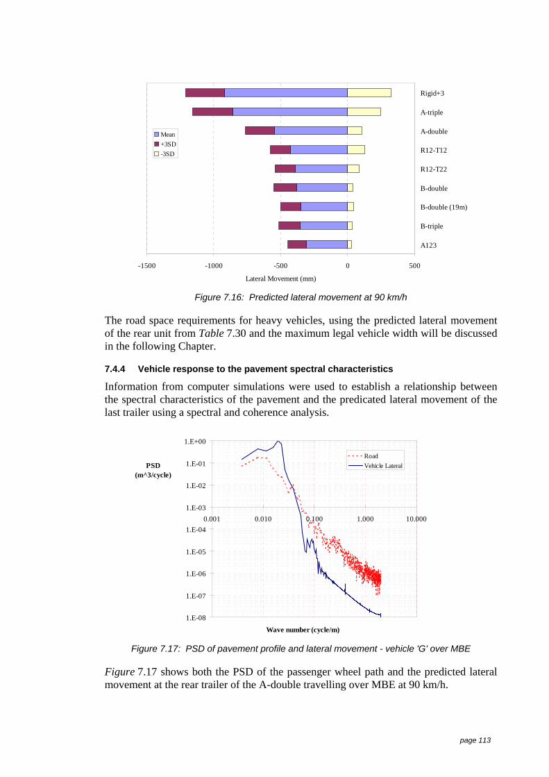
page 113
-1500 -1000 -500 0 500
A123
B-triple
B-double (19m)
B-double
R12-T22
R12-T12
A-double
A-triple
Rigid+3
Lateral Movement (mm)
Mean+3SD-3SD
Figure 7.16: Predicted lateral movement at 90 km/h
The road space requirements for heavy vehicles, using the predicted lateral movementof the rear unit from Table 7.30 and the maximum legal vehicle width will be discussedin the following Chapter.
7.4.4 Vehicle response to the pavement spectral characteristics
Information from computer simulations were used to establish a relationship betweenthe spectral characteristics of the pavement and the predicated lateral movement of thelast trailer using a spectral and coherence analysis.
1.E-08
1.E-07
1.E-06
1.E-05
1.E-04
1.E-03
1.E-02
1.E-01
1.E+00
0.001 0.010 0.100 1.000 10.000
Wave number (cycle/m)
PSD(m^3/cycle)
RoadVehicle Lateral
Figure 7.17: PSD of pavement profile and lateral movement - vehicle 'G' over MBE
Figure 7.17 shows both the PSD of the passenger wheel path and the predicted lateralmovement at the rear trailer of the A-double travelling over MBE at 90 km/h.

page 114
0.E+00
2.E-01
4.E-01
6.E-01
8.E-01
1.E+00
0.000 0.020 0.040 0.060 0.080 0.100
Wave number (cycle/m)
PSD(m^3/cycle)
RoadVehicle Lateral
Figure 7.18: PSD of pavement profile and lateral movement - vehicle 'G' over MBE
Figure 7.19 shows the same PSD data as in Figure 7.18 presented with a linear verticalscale. This scaling allows the dominant frequencies and amplitudes to be shownclearly, and it can be seen that the lateral movement of the rear trailer has a dominantresponse at 0.02 cycles/m and the passenger wheel path at approximately0.008 cycles/m.
0.0
0.2
0.4
0.6
0.8
1.0
0.000 0.020 0.040 0.060 0.080 0.100
Wave number (cycle/m)
Coherence
Figure 7.19: Coherence between the predicted lateral movement and the pavement profile
The coherence plot in Figure 7.19 confirms that there is no linear relationship betweenthe passenger wheel profile and the lateral movement at the rear trailer for the A-doubleat 90 km/h - there is low coherence at both the dominant responses, 0.02 and0.008 cycles/m.
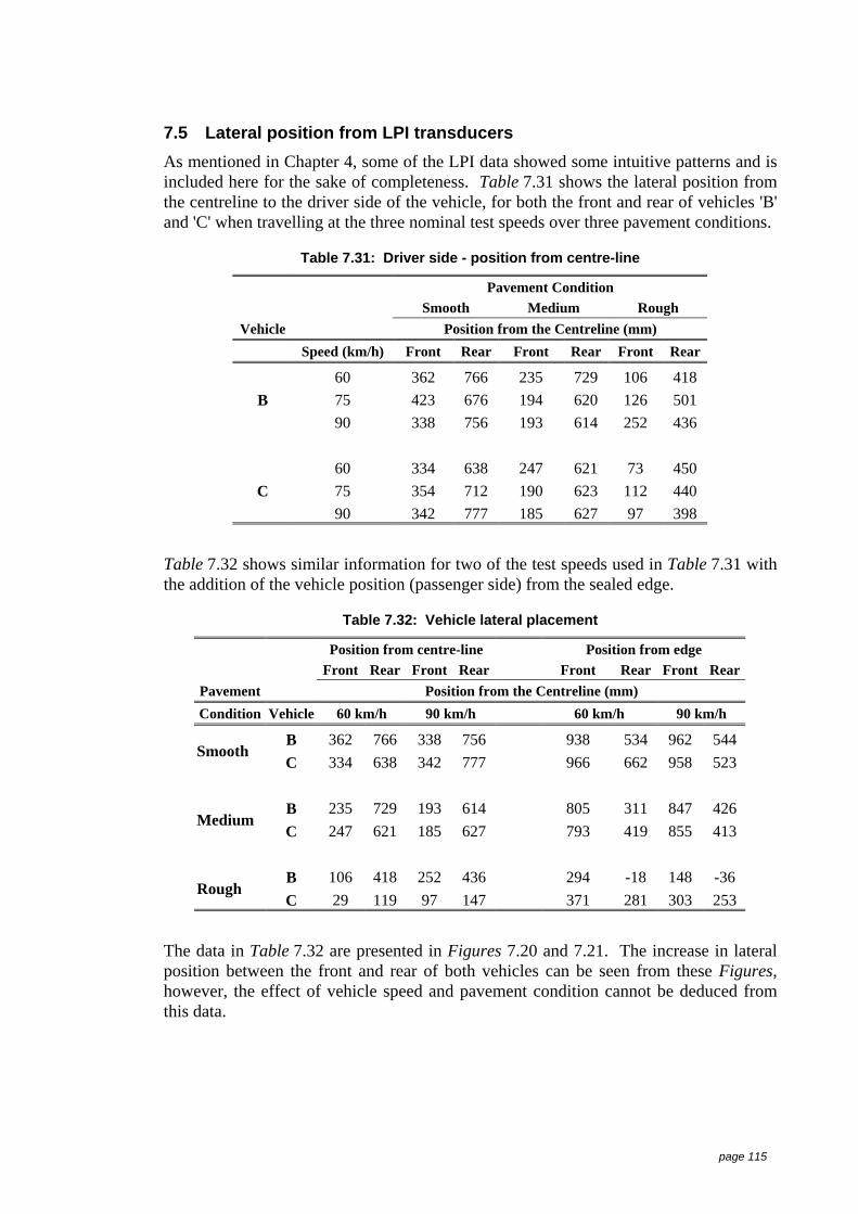
page 115
7.5 Lateral position from LPI transducersAs mentioned in Chapter 4, some of the LPI data showed some intuitive patterns and isincluded here for the sake of completeness. Table 7.31 shows the lateral position fromthe centreline to the driver side of the vehicle, for both the front and rear of vehicles 'B'and 'C' when travelling at the three nominal test speeds over three pavement conditions.
Table 7.31: Driver side - position from centre-line
Pavement ConditionSmooth Medium Rough
Vehicle Position from the Centreline (mm)Speed (km/h) Front Rear Front Rear Front Rear
60 362 766 235 729 106 41875 423 676 194 620 126 501B90 338 756 193 614 252 436
60 334 638 247 621 73 45075 354 712 190 623 112 440C90 342 777 185 627 97 398
Table 7.32 shows similar information for two of the test speeds used in Table 7.31 withthe addition of the vehicle position (passenger side) from the sealed edge.
Table 7.32: Vehicle lateral placement
Position from centre-line Position from edgeFront Rear Front Rear Front Rear Front Rear
Pavement Position from the Centreline (mm)Condition Vehicle 60 km/h 90 km/h 60 km/h 90 km/h
B 362 766 338 756 938 534 962 544Smooth
C 334 638 342 777 966 662 958 523
B 235 729 193 614 805 311 847 426Medium
C 247 621 185 627 793 419 855 413
B 106 418 252 436 294 -18 148 -36Rough
C 29 119 97 147 371 281 303 253
The data in Table 7.32 are presented in Figures 7.20 and 7.21. The increase in lateralposition between the front and rear of both vehicles can be seen from these Figures,however, the effect of vehicle speed and pavement condition cannot be deduced fromthis data.

page 116
0
100
200
300
400
500
600
700
800
900
1000
Smooth Medium Rough
Road Condition
Distancefrom
Centreline(mm)
60 km/h75 km/h90 km/h
Front
Rear
Front
Rear
Front
Rear
Figure 7.20: Driver side lateral position from centreline - vehicle 'B'
It is shown in both Figures 7.20 and 7.21 that the driver consistently placed the front ofthe vehicle a larger distance from the centreline on the smooth road than on both themedium and rough roads. This could be explained by:
1) the smooth road having a wider sealed lane width (3.8 m), in contrast to a 2.9 mwide lane width for the rough road (see Table 4.3), and the driver centring thevehicle in the lane;
2) the driver positions the hauling unit such that the in-side (passenger side) of the reartrailer remains on the sealed pavement and does not track on the shoulder.
0
100
200
300
400
500
600
700
800
900
1000
Smooth Medium Rough
Road Condition
Distancefrom
Centreline(mm)
60 km/h75 km/h90 km/h
Front
Rear
Front
Rear
Front
Rear
Figure 7.21: Driver side lateral position from centreline - vehicle 'C'
7.5.1 Significance of independent variables
To establish the significance of the lateral position of the rear of the vehicles as shownin Figures 7.20 and 7.21, an ANOVA was conducted on the rear position data presented

page 117
in Table 7.31 as the dependent variable. The independent variables were the vehicletype (vehicle 'B' and 'C'), lane width vehicle speed and IRI.
Table 7.33 summarises the regression statistics from the MLR and shows that 90% ofthe observed variation in the lateral position is explained by the combination of thethree variables; vehicle type (vehicle 'B' and 'C') lane width and VSR.
Table 7.33: MLR Lateral position in the lane - regression statistics
Multiple R 0.95R Square 0.90
Adjusted R Square 0.87Standard Error 46.62Observations 18
The ANOVA output from the MLR is given in Table 7.34 which shows that theregression coefficients are not equal to zero, F(3,14)=29.3, p<0.001, and that the lanewidth is a very significant predictor of lateral position p<0.001. The independentvariables vehicle type and speed are not statistically significant. However, thecombination of these four parameters provides a good prediction of the lateral positionof the rear trailer in the lane.
As mentioned earlier the standardised values for the coefficients allow the relativeimportance of the coefficients to be identified. As shown in Table 7.34 under the Betavalues, the lane width and IRI are the highest contributors to the lateral positionfollowed by speed and the vehicle type.
Table 7.34: MLR lateral position in the lane - ANOVA statistics
df SS MS F Sign FRegression 4 252394 63099 29.03 0.0000Residual 13 28252 2173
Total 17 280646
Coefficients Standard Error Beta t Stat P-valueIntercept 3893 513 - 7.59 0.000
Vehicle type -26.3 35.5 -0.11 1.18 0.259Speed -0.20 1.0 -0.02 -0.20 0.847
IRI 664 138.7 3.99 4.79 0.000Lane width -1433 248.2 -4.81 -5.77 0.000
7.6 Road space requirementsThe total lateral envelope that a vehicle occupies as it travels in a straight line athighway speed, is termed the road space requirement - it is the sum of the vehicle widthat the rear plus the lateral deviation of the rear unit. Both road space and lane widthinformation is fundamental to assessing route access for heavy vehicles to maintain asafe environment for other road users and hence a prime input for the model guidelines.

page 118
Using the performance information on total lateral movements for the vehicle used inthe second series of field experiments and the maximum legal width of a heavy vehicleof 2.5 m, the road space requirements for these vehicles and their suitability to usevarious routes can be estimated.
Information presented in Table 7.1 shows that for the A-double (vehicle 'G') the rear ofthe trailer has moved laterally within a total range of approximately 370 mm withreference to the hauling unit when travelling over the MBE road at 90 km/h. The roadspace requirement for this vehicle is therefore 2.9 m (2.5 + 0.37). This does notconsider the lateral movement of the hauling unit, which is estimated to be 115 mm(from Table 7.22) maximum movement for this vehicle over this test section.
Similarly, information from Table 7.7 for the truck-trailer (vehicle 'H') shows that theroad space requirements for this vehicle over the MBE road at 90 km/h is 2.8 m (2.5 +0.28). Again this does not consider the lateral movement of the hauling unit , which isestimated to be 148 mm (from Table 7.23) maximum movement for this vehicle overthis test section.
It should be noted that during the field experiments the data was collected under idealconditions (during daylight hours, dry roads, relatively low traffic volumes and thedrivers were well rested), and the results from this study were the 'best possible' andmay not be representative for vehicles operating in adverse conditions.
Austroads (1993) suggests that the design lane and shoulder widths for rural undividedsealed roads should be based on traffic volumes, as presented in Table 7.35.
Table 7.35: Recommended lane and shoulder widths
Design Traffic Volumes(AADT)
Numberof lanes
Lane width(m)
Shoulder Width(m)
< 150 1 3.5 1.5 - 2.5150 - 500 2 3 1 - 1.5
500 - 1,000 2 3 - 3.5 1 - 2> 1,000 2 3.5 1 - 3
source: Austroads (1993)
NB: This information is extracted from Austroads (1993) and it should be noted that it is givenwith caveats for roads with high heavy vehicle traffic volumes and mountainous countryetc.
The information presented in Table 7.35 suggests that a minimum lane width of 3 m isrequired for a two-lane low volume road. Given that the A-double requires a road spaceof 2.9 m when travelling over the medium test section at 90 km/h, only 100 mm (lessthan 4%) of the available road space, remains before the adjacent lane is encroached.Similarly the truck-trailer requires a road space of 2.8 m when travelling over themedium test section at 90 km/h, this leaves 200 mm available before the adjacent lane isencroached.
There are no pavement condition criteria associated with the recommended lane widths.Without this information it appears that a 3 m lane width is marginal for the safeoperation for the A-double. It also should be noted that the data collected for this studywas on straight road sections and information on the influence of curves is required tomake further judgements on the suitability of the A-double to safely operate onpavements with 3 m lane widths.

page 119
7.7 SummaryInformation acquired during the field experiments provided data for a number ofdifferent analyses (including spectral analysis, coherence, multi-linear regression andanalysis of variance). It was found that there was a low correlation between the LPIdata and any of the independent variables; vehicle speed, vehicle type, pavementcondition or VSR. It was therefore concluded that the LPI device was not providingconsistent valid lateral movement data therefore this data was not used for the primeinput to the model route selection guidelines.
However, the lateral position data acquired with the LPI's for vehicles 'B' and 'C' wereanalysed to identify the relationship between the vehicle position in the lane (driverbehaviour) and vehicle type, vehicle speed and IRI. The results from this analysisshowed that the lane width was the most significant parameter in determining theposition of the trailer in the lane.
Furthermore, some useful relationships were established between the measured lateralacceleration and the independent variables. Data from vehicles 'A', 'B', and 'C' wereanalysed as a sub-set of the series I vehicles and this showed that the vehicle type is amore significant predictor of lateral movement than VSR for this vehicle sub-set.
Vehicle performance information extracted from the video-based measurements fromthe second series of field experiments provided base-line data to compare estimated andpredictive methods of vehicle lateral movements. Analysis of data showed that both thetest vehicles ('G' and 'H') produced greater lateral movement travelling over the MBEroad than the RCW road surface. Whilst there was an insufficient sample of pavementsurface conditions (profiles and crossfall) to statistically identify the contributors to thisapparent anomaly, possible reasons for this could be the difference in wheelpathprofiles, the wavelength characteristics (spectral information that was present in thepavement that excited the vehicles but was not identified by the IRI index) or highercrossfall characteristics. It was also shown that the VSR was a significant predictor oflateral movement for both these vehicles.
Estimates of lateral movement using a double integration technique were produced.Good correlations with the video-based data were found for both estimates using themeasured lateral acceleration with and without compensation for the trailer roll andcrossfall of the pavement.
The lateral movements at the hauling units were also estimated using the doubleintegration technique. It was shown that the lateral movement at the hauling unit didnot provide a significant contribution to the lateral movement at the rear trailer. Thismeans that something else other than the steering activity is the major contributor to thelateral movement of the rear trailer.
Analysis of the data from computer simulations showed that the number of articulationsin a vehicle combination was the most significant predictor of lateral movement overthe GCM and overall length (OAL). It also showed that the pavement crossfall has amajor effect of vehicle lateral position, which is greater for longer vehicles.
Using the simulation lateral movement data and the pavement profile measured in thepassenger wheelpath, a frequency domain coherence analysis showed that there was nolinear relationship between these 2 parameters when the vehicle was travelling over theMBE road surface at 90 km/h. This means that something else, possibly in conjunction

page 120
with the pavement profile, is the major contributor to the lateral movement of the reartrailer.

page 121
8 Interpretation and Discussion
8.1 IntroductionAs described in the previous Chapter extensive statistical and graphical analyses wereconducted on the data collected and derived from both field experiments. Rigorousanalyses were also conducted on computer simulated lateral movement data. ThisChapter draws the outcomes of the analysis together and discusses the uses andapplication of the data towards developing the model route access guidelines.
To bring together the outcomes of this research it is important to consider thecontribution and shortcomings of each of the data sets to the prime elements of themodel guidelines as identified in the Research Aims in Chapter 3.
The concept of assessing route access based on the road space requirements of a vehiclecould be considered as a matrix of vehicle type/length, pavement conditionroughness/profile and lane width, as shown in Figure 8.1. The cells of the matrixindicate the maximum speed that each vehicle type would be permitted to travel overthe route with the pavement condition and lane width indicated. This concept could beused for a road or vehicle based approach to 'match the vehicle to the road' which wouldprovide an appropriate solution to route access to achieve safety priority goals.
Road Condition (roughness IRI)Smooth Medium Rough
Lane width (m)Vehicle Type <3 <3.5 >4 <3 <3.5 >4 <3 <3.5 >4Single articulatedA-doubleA-tripleTruck-trailerTruck-trailerB-doubleB-tripleRigid-plus-three
These cells could contain the maximum speed for eachvehicle type to travel on each of the pavements withidentified characteristics.eg. 80 km/h for an A-triple travelling over a medium
roughness pavement with a 3 m lane width.
Figure 8.1: Route access guidelines matrix concept
Given that the major purpose for developing access guidelines is to provide increasedefficiency for the transport industry, and that transport operators are able to respondwith improved vehicle designs quicker than effective changes to the infrastructure, itfollows that operators need information on the requirements and criteria for access tospecific routes. The following example illustrates the matrix concept:-

page 122
'if the road space requirement for a vehicle combination with a certain freight typeover a certain route exceeded the available lane width at the posted speed limit,then it may be possible to reduce the lateral movement of the rear trailer byreducing the maximum allowable speed for that vehicle, or alternatively, thevehicle combination be changed by removing a trailer, or using B-coupledtrailers.'
The initial research program was structured to collect lateral performance informationfrom five common vehicle types to provide a fundamental input into the prime aim ofthis study - the development of model guidelines for determining route access for heavyvehicles. However, due to the limitations of the lateral position indicator (LPI) device,the outputs from the first field experiments did not provide the information to developmodel guidelines. Subsequent field experiments were carried out using a reducednumber of vehicles which provided definitive lateral performance information for twovehicle types. Data from a small vehicle sample diminished the application of this dataset to the model guidelines.
As shown in the previous Chapter useful information was extracted from a sub-set ofthe data recorded during the first series of field experiments. Information providedfrom computer simulations was used to confirm the trends and outcomes from theanalysis of this data sub-set.
The following section outlines the contribution of the data to the model guidelines andthe other aims of the study.
8.2 Contribution to the model guidelinesAn overall objective of any performance-based regulatory scheme or guidelines is that asafety neutral or positive outcome is achieved and this is a clear objective of this study:-to use the excursions of the vehicles into adjacent lanes as a means of determining routeaccess.
A complete performance-based route access system for heavy vehicles should includesufficient measures to embrace all vehicle performance characteristics. A list ofperformance-based measures were given in Chapter 2 (Table 2.1), however, as aminimum, vehicle parameters such as low and high-speed off-tracking, rollover stabilityand lane encroachment need to be considered when assessing the suitability of a vehiclecombination for route access. Until a suite of performance characteristics have beendeveloped and accepted then the model guidelines as outlined could be used to assistwith determining route access for heavy vehicles in the interim.
Data collected and used for this study provided a contribution to the body of knowledgeon vehicle dynamics in the route access area and an embryonic input to develop routeaccess guidelines for heavy vehicles. The contribution of the information from thisstudy towards the model guidelines is outlined in this Chapter.
8.2.1 Vehicle type
Australian heavy vehicles in the 1980's generally consisted of a hauling unit towing 1, 2or 3 'standard' 13.7 m trailers; known as a single articulated, A-double or A-triplecombinations respectively. Trailers purpose-built for specific commodities and a pushfor higher freight efficiencies created new vehicle types which were generally betterperforming than the standard combination vehicles. The improved performance ofthese new vehicles lead to operators seeking access to non-traditional routes to further

page 123
improve freight efficiencies. Hence route access for a specific vehicle type became anissue for the transport industry. It has been clear from the outcomes of this study thatvehicle type is the major influence of lateral movement and hence a prime input intoroutes access guidelines.
As expected, it was shown from the analysis that the magnitude of lateral movementwas different for each vehicle type. In general the data showed that longer vehiclesproduced greater lateral movement at the rear of the last trailer. There was strongevidence that the vehicle type has a first-order effect on the lateral movement of the reartrailer. This is illustrated with the data from the field experiments where it was shownthat an A-double with an OAL of 33 m produced greater lateral movement than a 17 mlong truck-trailer.
It was also shown that increasing the number of trailers (and hence the number ofarticulations) also increases the lateral movement of the rear trailer.
8.2.1.1 Discussion
There was insufficient data to identify the effect of actual trailer length on the lateralmovement at the rear trailer. Assessing the influence of the trailer length was not anaim of this study as at the time of developing the research program, the majority oftrailers in the vehicle fleet were around the maximum 'S' dimension of 9.5 m, and it wasdifficult to obtain test units with variations in length for a controlled experiment. It wasalso considered too specific without knowing the future trends in trailer design toincorporate various length trailers in this experimental design.
The number of articulations and the number of trailers in a vehicle combination arecomplementary, therefore it is not possible in a field study of vehicle dynamics toseparate and identify the effect of each parameter on overall vehicle dynamics.
Given the small sample in the second series of field experiments it is difficult to showstatistically if the larger lateral movement was due to the vehicle length, the couplingtype or draw bar length. The confounding of dependent co-variables did not permit theinfluence of these effects to be isolated. However, the recorded data did clearly showthat increasing the vehicle length (adding standard trailers) increased the lateralmovement. Conversely B-coupled trailers reduced the lateral movement as thesecoupling types reduced the number of articulations and improved general dynamics byintroducing roll coupling between vehicle units.
The effect of drawbar length could be studied using computer simulations. For A-double and A-triple combination vehicles, drawbar lengths are generally not subject tolarge variation, and are generally between 4-5 m long. Using 'standard' 9.5 m 'S'dimension trailers, the drawbar length is selected to provide the maximum combinationOAL length of 36.5 m and 53.5 m for A-double and A-triple combination vehiclesrespectively. By contrast the drawbar lengths used with truck-trailers are subject togreater variation. These vehicles are generally designed to achieve the axle load limitsfor specific freight and the drawbar length to meet ADR 43/03, ie. not exceed 8.5 m fora trailer having a single axle group or not exceeding 5 m for others. For truck-trailercombinations using 4-axle trailers, the jurisdictions have effectively applied drawbarlength rules based on axle mass (Queensland Transport, 1998).

page 124
8.2.1.2 What's missing
To provide comprehensive information to develop model guidelines further data onnew/innovative purpose built vehicle types is required. This information can beobtained via computer simulation if the appropriate pavement profile information isavailable. An alternative is to use a minimum instrumentation system (describedbelow), and numeric processing to obtain performance information specific to thevehicle under test on the specific route.
8.2.1.3 Contribution to the model guidelines for route access
It has been shown that vehicle type is a prime consideration when assessing route accessand therefore must be a key input into the model guidelines.
When further performance information has been collected for a number of vehicles ineach vehicle class over a range of operating conditions such as speed, vehiclesuspension types, freight and pavement types, it would be possible to determine thevariation in lateral movement over different pavement conditions for each vehicle class.From this information it may be possible to develop the simplified matrix of lateralmovement for each vehicle class over a range of pavement types (as illustrated inFigure 8.1). However, this would require an acceptable method of rating pavementcondition for heavy vehicles, as it has been shown that the commonly used IRIpavement roughness index does not provide appropriate pavement classifications forheavy vehicles. Once a 'truck index' is developed and accepted, implementing thesimplified matrix would provide 'desk top' assessment and reduce the cost to thetransport industry when deciding routes and vehicle types.
8.2.1.4 Needs and future work
The data collected for this study did show that vehicle type is a major contributor tolateral movement, however, the influence of vehicle elements such as wheelbase ordraw bar length on overall lateral movement were not able to be extracted. Theseelements may only have secondary importance in overall vehicle lateral movement andtheir importance could be determined with a further experimental program on theeffects of the variations in these parameters on the overall vehicle lateral movement.
8.2.2 Vehicle speed
The effect of vehicle speed on the level of lateral movement was clearly shown, ie. thehigher the vehicle speed the larger the lateral movement. However, it was clearlyshown that over certain pavement types the truck-trailer combination produced largerlateral movement at 90 km/h, than 100 km/h. This effect was not evident from the datameasured for the A-double, possibly because the maximum test speed for this vehiclewas 90 km/h or this phenomenon is only associated with short wheel-base vehicle units.Collecting data at test speeds over 90 km/h was not part of the original experimentaldesign, however, it was decided to collect extra data as the truck-trailer was capable oftravelling at a higher speed and there was sufficient time available. This informationprovided an important outcome of this study.
8.2.2.1 Discussion
The notion of applying a variety of maximum speed restrictions to each vehicle or eachvehicle type may have practical limitations and could impact on traffic flow and hencehave an undesirable impact on safety. Whilst vehicle speed was an important

page 125
contributor to the vehicle lateral movement, the practicality of implementing a variablespeed limit scheme would need to be thoroughly considered in terms of safety beforeimplementation.
8.2.2.2 What's missing
As highlighted earlier, the effect of vehicle speed on the level of lateral movement wasclearly shown from the data acquired during the field experiments, however, it was alsoshown that over certain pavement types the truck-trailer combination produced largerlateral movement at 90 km/h, than 100 km/h. To have a comprehensive data set whendeveloping the route access guidelines matrix, information to resolve this phenomenonis required.
8.2.2.3 Contribution to the model guidelines for route access
Notwithstanding the practical and safety implications of different speed limits forvarious vehicle classes raised above, vehicle speed is a prime contributor to vehiclelateral movement, in general, increasing vehicle speed produces a larger lateral vehiclemovement. A balance between these two apparently conflicting aspects needs to beconsidered when implementing route access guidelines as vehicle speed is also a keyinput into the model guidelines and is a prime consideration when assessing routeaccess as well as other safety considerations.
8.2.2.4 Needs and future work
As described above, further information is required to resolve the phenomenon ofgreater lateral movement at a slower speed as measured for the truck-trailercombination. This may be a characteristic pertinent to truck-trailer vehicles due to theshort trailer wheelbase and the relatively long drawbar length. Consequently there arestrong links between vehicle speed and vehicle type which are central to the guidelinesfor route access.
8.2.3 Pavement roughness
The lateral movements at the rear of the last trailers were smaller over the smooth thanthe medium or rough pavement sections for most vehicle types used for the fieldexperiments.
The significance of the pavement roughness (IRI) on the vehicle lateral movement wasclearly shown from the analysis that was conducted on the video-based lateralmovement data.
Whilst this statistical evidence shows that pavement roughness contributes to vehiclelateral movement, the measured data for both the A-double and the truck-trailer vehiclesshowed a higher movement over the medium than rough pavement sections. Thisindicates that these vehicles respond to the variation in the pavement profile in adifferent manner than the quarter car model that is used to compute the IRI roughnessindex from the pavement wheelpath profiles.
Whilst there was clear evidence that pavements with higher roughness indices causemore lateral movement, there was no clear evidence on the increase of lateral movementof the rear trailer travelling over pavements with IRI values greater than 3.
A spectral analysis of the pavement profile and computer simulated lateral movement atthe rear trailer of the A-double showed that the peak energies occurred at different

page 126
wavenumbers. This means that the vehicle lateral movement is not directly excited bythe variation in the pavement profile (no linear relationship) or there is a combination ofelements which form a complex relationship which is beyond the scope of this study. Acoherence analysis confirmed that there was no linear relationship between these twoparameters. This is a major finding from this study and a subject for future research asit indicates that a better understanding of the excitation of vehicle over rough roads isrequired.
8.2.3.1 Discussion
As highlighted earlier under section 8.2.1, to develop model guidelines and desk-topassessment capability, performance information for a number of vehicles in eachvehicle class under a range of operational conditions is required. In order to determinethe scope and operational conditions that may be required to develop the assessmentcapability, information on the characteristics of routes that heavy vehicles are likely touse is required.
In light of the information presented in Section 2.6 on the proportion of Australianroads with roughness levels greater than IRI 4, and the findings by Thoresen on heavyvehicle speed reduction over roads with high roughness levels, there is a case to suggestthat information to establish a general desk-top assessment capability could be limitedto vehicle lateral performance information for vehicles travelling over pavement typeswith roughness levels not greater than IRI 4. The collection and collation of data todevelop this matrix is not a trivial task and would require broad consultation with allsectors of the transport industry. Nevertheless, as shown from this study it would beimportant to ensure that any further work in this area should use pavements that containa range of wavelength spectral components for each IRI roughness level.
8.2.3.2 What's missing
As raised in Section 2.7 under Implementation issues for performance-based standard,there is no consistent terminology used in Australia when classifying or defining routes.A common definition and specification for pavements using an appropriate method forheavy vehicles is required for a consistent route access guideline system to beimplemented. Such definitions should include a measure of pavement spectralcharacteristics and an appropriate truck response index.
8.2.3.3 Contribution to the model guidelines for route access
Information from the measured data suggests that pavement spectral characteristics areimportant contributors to the lateral movement of heavy vehicles. Furthermorepavement roughness is clearly an important element in the model guidelines for routeaccess. However, more work is required on defining or categorising pavementroughness condition for route access for various vehicle types and the establishment andacceptance of an appropriate truck pavement response index is also required.
8.2.3.4 Needs and future work
There is an intuitive propensity to believe that pavements with high roughness causelarger lateral movement of the rear trailer of a vehicle combination. There is no strongevidence from the data collected for this research to confirm this relationship, as therewas no clear relationship between the lateral movement of vehicles travelling overpavements with an IRI value greater than 3.
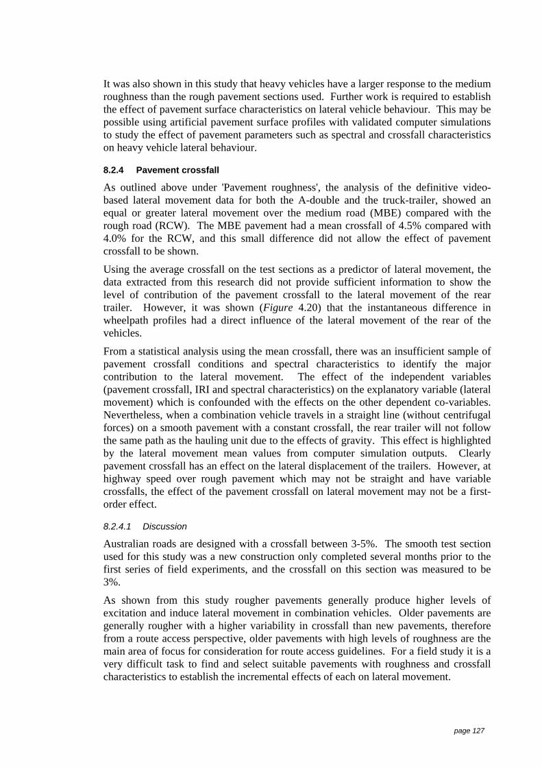
page 127
It was also shown in this study that heavy vehicles have a larger response to the mediumroughness than the rough pavement sections used. Further work is required to establishthe effect of pavement surface characteristics on lateral vehicle behaviour. This may bepossible using artificial pavement surface profiles with validated computer simulationsto study the effect of pavement parameters such as spectral and crossfall characteristicson heavy vehicle lateral behaviour.
8.2.4 Pavement crossfall
As outlined above under 'Pavement roughness', the analysis of the definitive video-based lateral movement data for both the A-double and the truck-trailer, showed anequal or greater lateral movement over the medium road (MBE) compared with therough road (RCW). The MBE pavement had a mean crossfall of 4.5% compared with4.0% for the RCW, and this small difference did not allow the effect of pavementcrossfall to be shown.
Using the average crossfall on the test sections as a predictor of lateral movement, thedata extracted from this research did not provide sufficient information to show thelevel of contribution of the pavement crossfall to the lateral movement of the reartrailer. However, it was shown (Figure 4.20) that the instantaneous difference inwheelpath profiles had a direct influence of the lateral movement of the rear of thevehicles.
From a statistical analysis using the mean crossfall, there was an insufficient sample ofpavement crossfall conditions and spectral characteristics to identify the majorcontribution to the lateral movement. The effect of the independent variables(pavement crossfall, IRI and spectral characteristics) on the explanatory variable (lateralmovement) which is confounded with the effects on the other dependent co-variables.Nevertheless, when a combination vehicle travels in a straight line (without centrifugalforces) on a smooth pavement with a constant crossfall, the rear trailer will not followthe same path as the hauling unit due to the effects of gravity. This effect is highlightedby the lateral movement mean values from computer simulation outputs. Clearlypavement crossfall has an effect on the lateral displacement of the trailers. However, athighway speed over rough pavement which may not be straight and have variablecrossfalls, the effect of the pavement crossfall on lateral movement may not be a first-order effect.
8.2.4.1 Discussion
Australian roads are designed with a crossfall between 3-5%. The smooth test sectionused for this study was a new construction only completed several months prior to thefirst series of field experiments, and the crossfall on this section was measured to be3%.
As shown from this study rougher pavements generally produce higher levels ofexcitation and induce lateral movement in combination vehicles. Older pavements aregenerally rougher with a higher variability in crossfall than new pavements, thereforefrom a route access perspective, older pavements with high levels of roughness are themain area of focus for consideration for route access guidelines. For a field study it is avery difficult task to find and select suitable pavements with roughness and crossfallcharacteristics to establish the incremental effects of each on lateral movement.
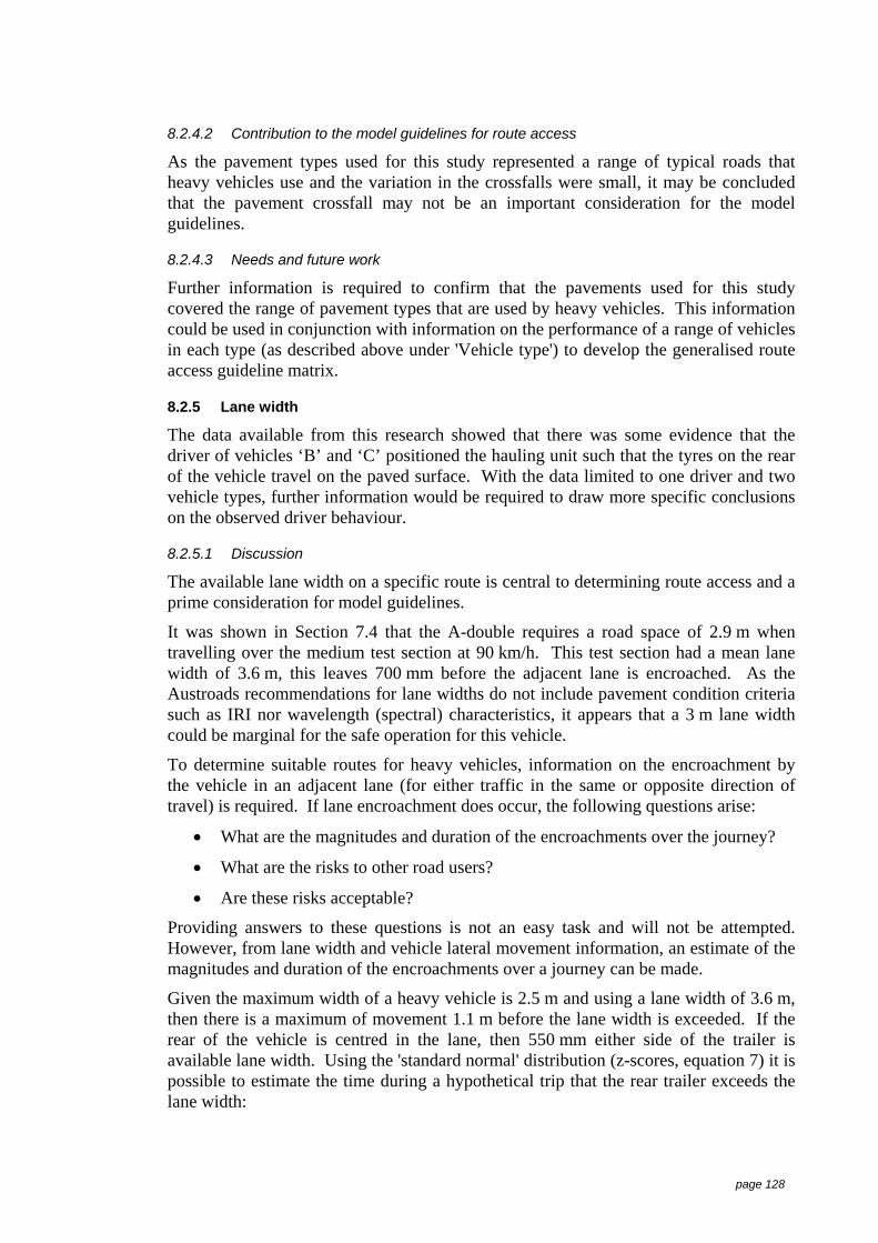
page 128
8.2.4.2 Contribution to the model guidelines for route access
As the pavement types used for this study represented a range of typical roads thatheavy vehicles use and the variation in the crossfalls were small, it may be concludedthat the pavement crossfall may not be an important consideration for the modelguidelines.
8.2.4.3 Needs and future work
Further information is required to confirm that the pavements used for this studycovered the range of pavement types that are used by heavy vehicles. This informationcould be used in conjunction with information on the performance of a range of vehiclesin each type (as described above under 'Vehicle type') to develop the generalised routeaccess guideline matrix.
8.2.5 Lane width
The data available from this research showed that there was some evidence that thedriver of vehicles ‘B’ and ‘C’ positioned the hauling unit such that the tyres on the rearof the vehicle travel on the paved surface. With the data limited to one driver and twovehicle types, further information would be required to draw more specific conclusionson the observed driver behaviour.
8.2.5.1 Discussion
The available lane width on a specific route is central to determining route access and aprime consideration for model guidelines.
It was shown in Section 7.4 that the A-double requires a road space of 2.9 m whentravelling over the medium test section at 90 km/h. This test section had a mean lanewidth of 3.6 m, this leaves 700 mm before the adjacent lane is encroached. As theAustroads recommendations for lane widths do not include pavement condition criteriasuch as IRI nor wavelength (spectral) characteristics, it appears that a 3 m lane widthcould be marginal for the safe operation for this vehicle.
To determine suitable routes for heavy vehicles, information on the encroachment bythe vehicle in an adjacent lane (for either traffic in the same or opposite direction oftravel) is required. If lane encroachment does occur, the following questions arise:
• What are the magnitudes and duration of the encroachments over the journey?
• What are the risks to other road users?
• Are these risks acceptable?
Providing answers to these questions is not an easy task and will not be attempted.However, from lane width and vehicle lateral movement information, an estimate of themagnitudes and duration of the encroachments over a journey can be made.
Given the maximum width of a heavy vehicle is 2.5 m and using a lane width of 3.6 m,then there is a maximum of movement 1.1 m before the lane width is exceeded. If therear of the vehicle is centred in the lane, then 550 mm either side of the trailer isavailable lane width. Using the 'standard normal' distribution (z-scores, equation 7) it ispossible to estimate the time during a hypothetical trip that the rear trailer exceeds thelane width:

page 129
σuxscorez −
=− (7)
where: x is the available lane widthσ is the sample standard deviationµ is the sample mean
As an example, using the information from computer simulations for the A-triple, alateral mean movement of -303, the available lane width is 853 (550 from the mean),and a standard deviation of 184 (from Table 7.29), the normal deviate is:
184303853 −
=− scorez = 2.99
The proportion or percentage that the z-score is greater than 2.99 can be obtained fromthe standard tables for the 'area under the standardised normal density'. In this case thearea in the upper tail of the distribution is of interest, and is the percentage of lateralmovement in a normal distribution that are more than 2.99 standard deviations abovethe mean, viz:
Pr(z > 2.99) = 0.0014
Considering the trailer movement is both inboard and outboard and drivers attempt toprevent the vehicle travelling off the shoulders, the probability of exceeding the lanewidth is the area in both the upper and lower tail of the distribution - which is twice thepredicted probability of 0.0014, ie. 0.28%. This means that for the A-triple travelling at90 km/h it is encroaching into adjacent lanes 0.28% of the time during the trip over theMBE road. For the vehicle travelling over this 1,000 m test section at 90 km/h (25 m/s)it exceeded the lane space for 0.11 sec. Extending this to an eight hour journey over aroad with similar roughness and wavelength characteristics, it would equate toexceeding the lane width for 80 seconds.
Exceeding the lane width for 80 seconds over an 8 hour journey (less than 2%) of thetotal time may not be considered to present a risk, however, the coincidence of theseexcursions and another vehicle need to be assessed to consider the risk to other roadusers.
8.2.5.2 What's missing
It should be noted that the data collected for this study was on straight road sections andinformation on the influence of curves is required to make further judgements on theneed to include or make allowances for vehicle lateral behaviour around curves in theaccess guidelines matrix.
8.2.5.3 Contribution to the model guidelines for route access
The pavement lane width is a fundamental consideration in determining access to aspecific route and information collected for this study showed that pavement lane widthwas the most significant parameter in determining the position of the trailer in the lane.
8.2.5.4 Needs and future work
Lateral movement information for vehicles negotiating curves on a range of pavementtypes is required to ensure that the route access guidelines include real worldconditions.

page 130
8.3 Minimum instrumentation to assess candidate vehiclesAs described in Section 5.5 a technique to measure vehicle lateral movement usingminimum instrumentation and relatively simple numeric processing was developed.The application of this technique was demonstrated by processing the recorded data andobtaining estimates of the lateral movement for each test vehicle used for this study.This information is presented in Chapter 7.
This technique uses an accelerometer mounted on the rear chassis of the last trailer tomeasure the lateral acceleration. If an accelerometer without inertial correction is usedthen the output signal will contain undesirable influences from several sources. Theseundesirable components can be removed by estimating the trailer chassis roll angle andthe crossfall of the pavement. The roll angle of the rear trailer is computed from thedifference in the driver and passenger side heights measured relative to the pavement by2 infra-red height measuring devices. These parameters were recorded along with thevehicle speed information for subsequent processing and numeric analysis to producean estimate of the lateral movement of the vehicle unit that the accelerometer is attachedto. A detailed analysis of this technique is presented in Chapter 7.
8.3.1 Discussion
Measuring pavement wheel path profiles using the Walking Profiler provided essentialaccurate data for this study. However, it was shown that it is possible to obtain vehiclelateral performance information without using the pavement profile information tocompensate for the crossfall of the pavement. Collecting pavement wheel path profilesusing this method is time consuming and requires lane closure, omitting thisinformation from the data processing can provide good estimates of lateral movement ata reduced cost.
Initially information on the pavement crossfall and the trailer roll angle was used tocompensate for their influence on the measured lateral acceleration. It was shown thatgood estimates of the lateral movements could be obtained without using the pavementcrossfall or the chassis roll angles.
8.3.2 Contribution
This method is considered appropriate to provide a simple minimum instrumentationmethod to measure the lateral movement of vehicles. In its simplest form, datacollected from more than one vehicle type travelling over the same pavement could beused for comparative or assessment purposes.
8.3.3 Needs and future work
It was shown from the data recorded across all combinations of vehicle speed and roadconditions for the car-carrying A-triple that the estimated lateral movements using theminimum instrumentation and relatively simple numeric processing appears to berelative constant. However, it was noted that the standard deviation values of the lateralacceleration recorded at the rear of the rear trailer were generally larger than those forthe other A-triple over the same test roads. It was observed during the experiments thatthe car-carrying A-triple was driven very conservatively. These two pieces ofinformation appear to be contradictory. However, no explanation was found for theserelatively constant estimates for lateral movement of the last trailer. Further work isrequired to resolve this anomaly and to establish the robustness of this method ofestimating the lateral movement of heavy vehicles.

page 131
8.4 Provision of performance data to validate computer models andlateral performance simulations
Outputs from this research provided definitive performance information to validatecomputer models and lateral movement simulations.
8.4.1 Discussion
The computer simulation outputs were only validated using measured data collected forthe A-double at two test speeds. Therefore it could be argued that simulations producedusing speeds beyond the validation speeds need to be used with circumspection.
8.4.2 What's missing
Measured information from only one vehicle was used during computer modelling andlateral movement simulation validation.
Simulation lateral movement data provided for this study was generated using only theMBE road surface, therefore the effects of the pavement roughness could not beassessed. Some variability in the reference data (video-based lateral movement) forrepeat passes over the test sections, did not provide sufficient information to assess theabsolute accuracy of computer simulations. It is therefore difficult to establish theabsolute accuracy of the computer predicted lateral movement information.
8.4.3 Contribution
The lane-change data acquired during the rearward amplification tests were used tovalidate computer models, and subsequently the video-based lateral movementinformation was used to validate computer simulations for lateral movement. The useof this data allowed development of computer models and simulations of heavy vehiclestravelling over pavements with measured wheel path profiles. The computer simulatedlateral movement information was used for a number of related studies as mentioned inChapter 2.
8.4.4 Needs and future work
Simulated lateral movement information was only conducted for vehicles travellingover the medium roughness road (MBE). It was therefore not possible to determine theeffect of different pavement conditions on vehicle lateral performance. Further work istherefore required to convert the pavement wheelpath profiles measured for this studyinto a suitable form for computer simulations to enable lateral movement information tobe generated for these pavement profiles.
In addition it would be possible to study the effect of a wider range of pavementparameters such as spectral and crossfall characteristics on heavy vehicle lateralbehaviour using artificial pavement surface profiles as raised in Section 6.7. Thesestudies would only be meaningful if conducted with validated computer models andsimulations.
8.5 LimitationsA number of vehicle parameters have been identified that may influence the lateralmovement of heavy vehicles that were not part of the experimental design of this work.It is important that the influence of these and other parameters be considered whendeveloping route access guidelines. The following list identifies these parameters:

page 132
1) load CoG height;
2) vehicle suspension type (Air suspensions or variations in steel suspensions);
3) tyre types and tyre pressures;
4) the lateral position of the vehicle in the lane;
5) different drivers.
The effect of the vehicles operating on 'real world' roads with curves on the lateralmovement also needs to be considered. The test roads used for the experiments in thisstudy were selected to be straight to enable direct comparisons to be made without theeffect of the vehicle position when negotiating curves and the inclusion of lateralmovement on vehicles when negotiating curves would add another dimension to thestudy.
It was raised in Section 7.3 that during the field experiments the data was collectedunder ideal conditions (during daylight hours, dry roads, relatively low traffic volumesand the drivers were well rested), and the results from this study were the 'best possible'and may not be representative for vehicles operating in adverse conditions.
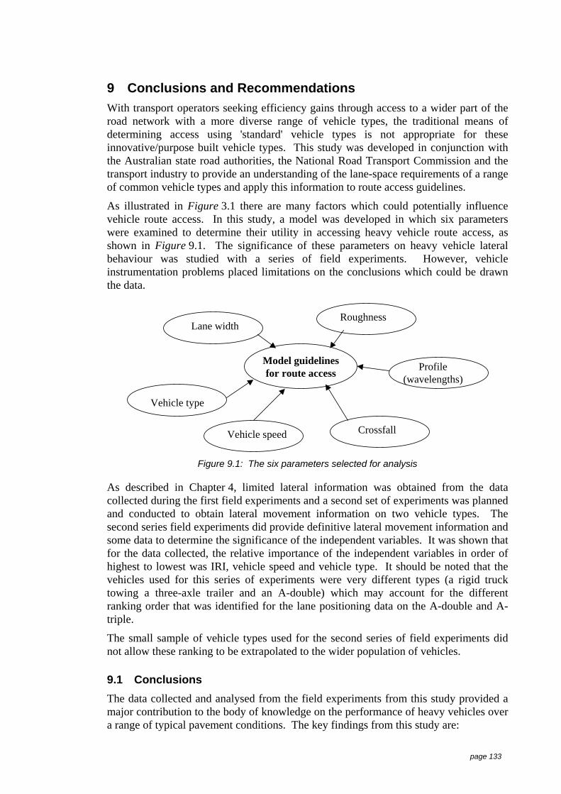
page 133
9 Conclusions and RecommendationsWith transport operators seeking efficiency gains through access to a wider part of theroad network with a more diverse range of vehicle types, the traditional means ofdetermining access using 'standard' vehicle types is not appropriate for theseinnovative/purpose built vehicle types. This study was developed in conjunction withthe Australian state road authorities, the National Road Transport Commission and thetransport industry to provide an understanding of the lane-space requirements of a rangeof common vehicle types and apply this information to route access guidelines.
As illustrated in Figure 3.1 there are many factors which could potentially influencevehicle route access. In this study, a model was developed in which six parameterswere examined to determine their utility in accessing heavy vehicle route access, asshown in Figure 9.1. The significance of these parameters on heavy vehicle lateralbehaviour was studied with a series of field experiments. However, vehicleinstrumentation problems placed limitations on the conclusions which could be drawnthe data.
Model guidelinesfor route access
Lane widthRoughness
Profile(wavelengths)
Crossfall
Vehicle type
Vehicle speed
Figure 9.1: The six parameters selected for analysis
As described in Chapter 4, limited lateral information was obtained from the datacollected during the first field experiments and a second set of experiments was plannedand conducted to obtain lateral movement information on two vehicle types. Thesecond series field experiments did provide definitive lateral movement information andsome data to determine the significance of the independent variables. It was shown thatfor the data collected, the relative importance of the independent variables in order ofhighest to lowest was IRI, vehicle speed and vehicle type. It should be noted that thevehicles used for this series of experiments were very different types (a rigid trucktowing a three-axle trailer and an A-double) which may account for the differentranking order that was identified for the lane positioning data on the A-double and A-triple.
The small sample of vehicle types used for the second series of field experiments didnot allow these ranking to be extrapolated to the wider population of vehicles.
9.1 ConclusionsThe data collected and analysed from the field experiments from this study provided amajor contribution to the body of knowledge on the performance of heavy vehicles overa range of typical pavement conditions. The key findings from this study are:

page 134
1) The magnitude of lateral movement was different for each vehicle type. In generallonger vehicles produced greater lateral movement at the rear trailer. There wasstrong evidence that the vehicle type has a first-order effect on the lateralmovement of the rear trailer, therefore vehicle type is a prime consideration whenassessing route access and is a key input into the model guidelines;
2) The effect of vehicle speed on the level of lateral movement was clearly shown, ie.the higher the vehicle speed the larger the lateral movement, strong links betweenvehicle speed and vehicle type are central to the guidelines for route access.However, it should be noted that an equal or greater lateral movement wasmeasured over the medium road compared with the rough road. Whilst furtherinformation is required to explore this apparent anomaly, possible causes or areasthat could contribute to this are the pavement surface spectral characteristics,difference in wheel path profiles, the pavement crossfall or the pavement roughnessof the test sections. The safety and practical implications need to be consideredwhen applying different speed limits for various vehicle classes when implementingroute access guidelines;
3) Pavement roughness was a key contributor to the vehicle lateral movement. Thelateral movement of the rear of the last trailer was smaller over the smooth than themedium or rough pavement sections for most vehicle types used for the fieldexperiments. Whilst there was statistical evidence that pavement roughnesscontributes to vehicle lateral movement, higher lateral movement at the rear of thevehicles was measured over the medium than rough pavement sections. Thisindicates that these heavy vehicles respond to the variation in the pavement profilein a different manner than the quarter car model that is used to compute the IRIroughness index from the pavement wheelpath profiles;
4) Whilst is was shown that the point-by-point pavement crossfall was a majorinfluence on the lateral movement of the last trailer, based on a statistical analysisof the data obtained from the small sample which only considered the averagecrossfall of each test section, the test sections used for this research did not providesufficient information to conclude statistically that pavement crossfall contributedto the lateral movement of the rear trailer. There was an insufficient sample ofpavement crossfall conditions and spectral characteristics to identify the majorcontribution to the lateral movement. The effect of the independent variables(pavement crossfall, IRI and spectral characteristics) on the explanatory variable(lateral movement) is confounded with the effects on the other dependent co-variables;
5) Limited lateral position information suggested that one driver of two vehicle typesposition the vehicles so that the tyres on the rear trailer track on the sealedpavement and not on the pavement shoulder.
9.2 RecommendationsThe need to develop guidelines to assist with the route selection for heavy vehicles wasraised in Chapter 3 and the contributions of each element were identified in Chapter 8.The structure, input needs and parameters to these guidelines became one of the aimscentral to this thesis.
The parameters identified as the key inputs into the model guidelines and the findingsfrom this study are (not necessarily in order of importance):

page 135
9.2.1 Vehicle type contribution to the model guidelines for route access
It has been shown that vehicle type is a prime consideration when assessing route accessand therefore is a key input into the model guidelines.
9.2.2 Vehicle speed contribution to the model guidelines for route access
Notwithstanding the practical and safety implications of different speed limits forvarious vehicle classes raised earlier, vehicle speed is a prime contributor to vehiclelateral movement, in general, increasing vehicle speed produces a larger lateral vehiclemovement. A balance between these two apparently conflicting aspects needs to beconsidered when implementing route access guidelines as vehicle speed is also a keyinput into the model guidelines and is a prime consideration when assessing routeaccess as well as other safety considerations.
9.2.3 Pavement roughness contribution to the model guidelines for route access
Information from the measured data suggests that pavement spectral characteristics areimportant contributors to the lateral movement of heavy vehicles. Furthermorepavement roughness is clearly an important element in the model guidelines for routeaccess. More work is required on defining or categorising pavement roughnessconditions for route access for various vehicle types and the establishment andacceptance of an appropriate truck pavement response index.
9.2.4 Pavement crossfall contribution to the model guidelines for route access
The range of pavement crossfalls on the test pavements used for the experimental stageof this study was small and further investigations are needed to establish therelationship between the magnitude of the crossfall and the effect on vehicle lateralmovement for the inclusion of this parameter in the model guidelines.
9.2.5 Lane width contribution to the model guidelines for route access
The pavement lane width is a fundamental consideration in determining access to aspecific route and information collected for this study showed that pavement lane widthwas the most significant parameter for drivers determining the position of the trailer inthe lane.
9.3 Further researchA number of questions have been raised from the findings of this research and furtherwork is recommended to resolve the following:
1) The influence of vehicle parameters such as wheelbase and draw bar length onoverall lateral movement requires addressing. These parameters may only havesecondary importance in overall vehicle lateral movement and the effects of thevariations in these parameters on lateral movement needs further investigation;
2) Information is required to resolve the phenomenon of greater lateral movement at aslower speed as measured for the truck-trailer combination. This may be acharacteristic pertinent to truck-trailer vehicles due to the short trailer wheelbaseand the relatively long drawbar length;
3) One of the main findings from this study was that the measured lateral movementof the rear of the last trailer was smaller over the rough than the medium roughness

page 136
pavement sections. Further work is required to establish the effect of pavementsurface characteristics on lateral vehicle behaviour;
4) Information on the influence of curves is required to make further judgements onthe importance of including performance on real-world roads in the route accessguidelines;
5) Information on vehicle lateral performance under a wider range of operatingconditions such as wet roads, night, heavier traffic volumes, driver fatigue and arange of drivers;
6) With the small sample of driver lateral lane placement behaviour, furtherinformation would be required with a larger sample of vehicles and drivers to drawmore specific conclusions;
7) Further research is also required on a wider range of pavement and vehicle types tosupplement the information from this study.
Therefore the following are recommendations for future research:
1) the effect of pavement surface spectral characteristics on the lateral movement ofthe rear trailer of a vehicle combination;
2) the effect of pavement surface crossfall on the lateral movement of the rear trailerof a vehicle combination;
3) the relationship between the pavement surface profile, specifically with IRI valuesgreater than 3, on the lateral movement of the rear trailer of a vehicle combination;
4) the effect of vehicle speed (and wheelbase filtering) on the lateral movement of therear trailer of a vehicle combination;
5) the influence of negotiating curves on the magnitude of lateral movement for heavyvehicles;
6) the vehicle lateral performance on a wider range of pavement and vehicle types isrequired to supplement the information from this study.
When further performance information has been collected for a number of vehicles ineach vehicle class over a range of operating conditions such as, speed, vehiclesuspension types, freight and pavement types, it would be possible to determine thevariation in lateral movement over different pavement condition for each vehicle class.From this information it may be possible to develop the simplified matrix of lateralmovement for each vehicle class over a range of pavement types (as outlined inFigure 8.1). However, this would require an acceptable method of rating pavementcondition for heavy vehicles, as it has been shown that the commonly used IRI indexdoes not provide appropriate pavement classifications for heavy vehicles therefore a'truck index' needs to be developed and accepted. Once developed and acceptedimplementing the simplified matrix would reduce the cost to the transport industrywhen deciding routes and vehicle types as it would provide 'desk top' assessment.
9.4 Further needsA number of questions have been raised from the findings of this research and thefollowing future need have been identified:

page 137
9.4.1 Vehicle type needs and future work
The data collected for this study did show that vehicle type is a major contributor tolateral movement, however, the influence of vehicle elements such as wheelbase ordraw bar length on overall lateral movement were not able to be extracted. Theseelements may only have secondary importance in overall vehicle lateral movement andtheir importance could be determined with a further experimental program on theeffects of the variations in these parameters on the overall vehicle lateral movement.
9.4.2 Vehicle speed needs and future work
As described above further, information is required to resolve the phenomenon ofgreater lateral movement at a slower speed as measured for the truck-trailercombination. This may be a characteristic pertinent to truck-trailer vehicles due to theshort trailer wheelbase and the relatively long drawbar length. Subsequently there arestrong links between vehicle speed and vehicle type which are central to the guidelinesfor route access.
9.4.3 Pavement roughness needs and future work
There is an intuitive propensity to believe that pavements with high roughness causelarger lateral movement of the rear trailer of a vehicle combination. There is no strongevidence from the data collected for this research to confirm this relationship, as therewas no clear relationship between the lateral movement of vehicles travelling overpavements with an IRI value greater than 3.
It was also shown in this study that heavy vehicles have a larger response to the mediumroughness than the rough pavement used in this study. Further work is required toestablish the effect of pavement surface characteristics (profile, roughness and crossfall)on lateral vehicle behaviour. It may be possible using artificial pavement surfaceprofiles with validated computer simulations to study the effect of pavement parameterssuch as spectral and crossfall characteristics on heavy vehicle lateral behaviour.
9.4.4 Pavement crossfall needs and future work
To confirm the pavements that were used for the field experiments for this studycovered the pavement types that are used by heavy vehicles, further information isrequired on the characteristics of a wider range of pavement types that are used byheavy vehicles. This information could be used in conjunction with information on theperformance of a range of vehicles in each type (as described above under vehicle type)to develop generalised route access guidelines.
9.4.5 Lane width needs and future work
It also should be noted that the data collected for this study was on straight roadsections and information on the influence of curves is required to make furtherjudgements on the suitability of the A-double to safely operate on pavements with 3 mlane widths.
With the data limited to one driver and two vehicle types, further information would berequired to draw more specific conclusions.

page 138
10 ReferencesALBERTA DEPARTMENT of HIGHWAYS and TRANSPORT, (1970). Report on the Testing
of Triple Trailer Combinations in Alberta. (Edmonton: Alberta Dept of Highways andTransport, Canada).
ARRB TR, (1995). Walking Profiler Instruction Manual. ARRB Transport Research (ARRBTR: Vermont South, Vic.).
AULTMAN-HALL, L. and HILL, M. L. (1999). Methodology for Evaluating Large TruckAccess to Intermodal and Other Facilities. Transportation Research Record, No.1653.(TRB: Washington, DC, USA).
AUSTRALIA GOVERNMENT, (1995). Road Transport Reform (Commercial vehicleStandards), Regulations. Statutory Rule, No. 55. (AGPS: Canberra ACT).
AUSTROADS, (1988). Guide to Traffic Engineering Practice. Part 9 - Arterial Road TrafficManagement. (Austroads: Sydney, NSW).
AUSTROADS, (1992a). Pavement Design Guide. A Guide to the Structural Design of RoadPavements. (Austroads: Sydney, NSW).
AUSTROADS, (1992b). Review of Vehicle Dimension Limits, Austroads Road UseManagement Program, RUM 3.B.39. (Austroads: Sydney, NSW).
AUSTROADS, (1992c). Austroads Bridge Design Code - Section Two-Code Design Loads,AP-15.2. (Austroads: Sydney, NSW).
AUSTROADS, (1993). Austroads Rural Road Design - Guide to the Geometric Design ofRural Roads, AP-1/89. (Austroads: Sydney, NSW).
AUSTROADS, (1994). Network Access Guidelines for Large Vehicles, Austroads Road UseManagement Program, RUM 3.E.75. (Austroads: Sydney, NSW).
AUSTROADS, (1995). Design Vehicles and Turning Path Templates, Austroads PublicationNo. AP-34/95 (Austroads: Sydney, NSW).
AUSTROADS, (1997). RoadFacts '96, (Austroads: Sydney, NSW).
AUSTROADS, (2000). RoadFacts, (Austroads: Sydney, NSW).
BANDER, J. L. (2000). Sequential Decision Problems Arising in Commercial VehicleOperations. Ph. D Thesis. (University of Michigan: Ann Arbor USA).
BENDAT, J. S. and PIERSOL, A.G. (1971). Random Data: Analysis and MeasurementProcedures. (Wiley-Interscience: New York, USA).
BILLING, J. R. (1992). A Discussion of Performance Standards for Configuration ofCommercial vehicles. Third International Symposium on commercial vehicle weightsand dimensions, Cambridge, UK. (Telford: London, UK).
CEBON, D. and NEWLAND, D.E. (1983). The Artificial Generation of Road SurfaceTopography by the Inverse FFT Method. Proc 8th IAVSD Symposium, "The Dynamics ofVehicles on Roads and Railway Tracks", Cambridge Massachusetts, pp29-42. (Swetsand Zeitlinger: Lisse, The Netherlands).
CLANCY, S. (2000). Time and Motion. Freight Vol. 33 Issue Number 9. (Freight TransportAssociation: Kent, UK).
Dataq (1993). DI-220 PGH/PGL, User Manual. (Dataq Instruments Inc: Ohio, USA).
DODDS, C. J. and ROBSON, J.D. (1973). The Description of Road Surface Roughness.Journal of Sound Vibration, 31(2), pp175-183. (Academic Press: New York, USA).

page 139
DODS, J. S. (1982). The ARRB Lateral Position Indicator. Australian Road Research Board,Technical Report ATM No 15. (ARRB TR: Vermont South, Vic.).
DTW, (1990). The Journal, Department of Transport and Works, Staff News Letter, October1990. (Department of Transport and Works: Darwin, NT).
DUELL, T. (1997). The ATEA Proving Ground Random Ride Facility. Army Technology &Engineering Agency, (ATEA: Maribyrnong, Vic.).
El-GINDY, M. (1992). The Use of Commercial Vehicle Performance Measures for Design andRegulation. DSC Vol. 44, Transportation Systems. (ASME: New York, USA).
ELISCHER, M. P. and PREM. H. (1997). Validation of Commercial Vehicle DynamicModelling Using ADAMS - Lane Change Manoeuvre. ARRB Transport Research,Contract Report OC6503V. Restricted circulation. (ARRB TR: Vermont South, Vic.).
ERVIN, R. D., FRANCHER, P. S., GILLESPIE, T. D., WINKLER, C. B. and WOLFE, A.(1978). Ad Hoc Study of Certain Safety-Related Aspects of Double-Bottom Tankers.Final report, Highway Safety Research Institute, University of Michigan. Report NoUM-HSRI-78-18. (UMTRI: Ann Arbor, Michigan, USA).
ERVIN, R. D. and GUY, Y. (1986a). Axioms Relating Truck Size and Weight To VehicleControllability. International Symposium on Commercial vehicle Weight & Dimensions,Kelowna, British Columbia. (RTAC: Ottawa, Canada).
ERVIN, R. D. and GUY, Y. (1986b). The Influence of Weights and Dimensions on theStability and Control of Heavy Trucks in Canada, Vol. 1 Part 1. (CanroadTransportation Research: Ottawa, Canada).
FANCHER, P.F. (1982). The Transient Directional Response of Full Trailers. SAE No 821259. Society of Automotive Engineers, Inc. (SAE: Warrendale PA, USA).
FANCHER, P. F. and MATHEW, A. (1990). Safety Implications of Various Configurations -Vol. 1: Technical report UMTRI-88-32, University of Michigan TransportationResearch Institute. (UMTRI: Ann Arbor, Michigan, USA).
GEORGE, R. M. (1994). Research Proposal - Performance-based Standard on the TrailingFidelity of Multi-Combination Vehicles. ARRB Transport Research Proposal, AP 045,Restricted circulation. (ARRB TR: Vermont South, Vic.).
GEORGE, R. M. (1996). Stability of High Vehicles. ARRB Transport Research, ContractReport to the National Road Transport Commission, No. CR C5546. (ARRB TR:Vermont South, Vic.).
GEORGE, R. M. (1997). Status Report - Road Network Access Standards for HeavyCommercial Vehicles - phase II. ARRB Transport Research, Contract Report toAustroads, No. CR OC6503. (ARRB TR: Vermont South, Vic.).
GEORGE, R. M. (1998). Workshops on a Commercial Vehicle Performance-BasedAssessment Scheme. ARRB Transport Research, Contract Report to Austroads, No. RE780306. (ARRB TR: Vermont South, Vic.).
GEORGE, R. M., ELISCHER, M. P. and PREM. H. (1998a). Road Network Access Standardsfor Heavy Commercial Vehicles. Proc. 5th Int. Symp. on Commercial vehicle Weightsand Dimensions. (ARRB TR: Vermont South, Vic.).
GEORGE, R. M., ELISCHER, M. P. and PREM. H. (1998b). Exemption Guidelines for Non-Standard Vehicles. Proc. 5th Int. Symp. on Commercial vehicle Weights andDimensions. (ARRB TR: Vermont South, Vic.).
GEORGE, R. M., ELISCHER, M. P. and PREM. H. (1998c). Exemption Guidelines for Non-Standard Vehicles. ARRB Transport Research, Contract Report to Austroads, No.OC6504. (ARRB TR: Vermont South, Vic.).

page 140
GEORGE, R. M., PREM, H., TAYLOR, R, and McLEAN, J. R, (1998d). Commercial VehicleAccess Strategy. ARRB Transport Research, Contract Report to Austroads, No. RC7037. (ARRB TR: Vermont South, Vic.).
GILLESPIE, T. D. (1985). Heavy Truck Ride. The thirty-first L. Ray Buckendale Lecture, SP-607. Society of Automotive Engineers, Inc. (SAE: Warrendale PA, USA).
GRIFFIN, M. J. (1990). Handbook of Human Vibration. Harcourt Brace Jovanovich.(Academic Press: London, UK).
HASSAN, R. A., and McMANUS, K. J. (2000). Truck Driver Perception as an Indication ofPavement Performance. Road Engineering Association of Asia, 10th Conference. (Shah:Alam Malaysia).
HEATH, A. N. (1989). Modelling and Simulation of Road Roughness. Proc 11th IAVSDSymposium, "The Dynamics of Vehicles on Roads and Railway Tracks", Ontario,Canada, pp 275-284. (Swets and Zeitlinger: Amsterdam, The Nertherlands).
ISO, (1995). International Organisation for Standardisation Mechanical Vibration - RoadSurface Profiles - Reporting of Measured Data, ISO/DIS 8608. (ISO: Geneva,Switzerland).
JOHNSTON, I. R. (1983). The Effects of Roadway Delineation on Curve Negotiation by BothSober and Drinking Drivers, Australian Road Research Board, Research Report ARR128. (ARRB TR: Vermont South, Vic.).
KORTÜM, W. and SHARP, R. S. (1993). Multibody Computer Codes in Vehicle DynamicSystems. Supplement to Vehicle System Dynamics, Vol. 22. (Swets and Zeitlinger:Amsterdam, The Netherlands).
LAND TRANSPORT, (1991). Road and Traffic Standards Information, No. 6, Revision 1,(Ministry of Transport: Wellington, New Zealand).
LITTLE, J. N., and SHURE, L. (1993). Signal Processing Toolbox. The MathWorks, Inc.(Nartick: Massachusetts, USA).
MADDOCK, J. (1988). A History of Road Trains in the Northern Territory. Kangaroo Press:(Kenthurst, NSW).
McLEAN, J. R., CAIRNEY, P. T., TAN, H.W. and GEORGE, R. M. (1995). Desirable RoadEnvironment Characteristics for Road Transport Vehicles. ARRB Transport Research,Contract Report TE 816. (ARRB TR: Vermont South, Vic.).
McLEAN, J. R. and RAMSAY, E. D. (1996). Interpretations of Road Profile Data: ARRBTransport Research, A discussion paper. WD AM 96/01. (ARRB TR: Vermont South,Vic.).
McMANUS, K. J., MANN, A. and EVANS, R. P. (1998). The Analysis of Road Roughnessand the Perception of Road Roughness. Proc. 5th Int. Symp. on Commercial vehicleWeights and Dimensions. (ARRB TR: Vermont South, Vic.).
NAASRA (1978). NATIONAL ASSOCIATION OF AUSTRALIAN STATE ROADAUTHORITIES. A Study of the Operation of Large Combination Vehicles (RoadTrains), Working Party Report No. 1, "Definitions, Dimensional Limitations, MechanicalRequirements and Operational Requirements". (NAASRA: Sydney, NSW).
NAASRA (1980). NATIONAL ASSOCIATION OF AUSTRALIAN STATE ROADAUTHORITIES. A Study of the Operation of Large Combination Vehicles (RoadTrains), "Guidelines for Route Selection for Road Trains". (NAASRA: Sydney, NSW).
NRTC, (1994). Restricted Access Vehicles. National Road Transport Commission TechnicalWorking Paper No. September 1994. (NRTC: Melbourne, Vic.).

page 141
NRTC, (1997). Assessment of Truck-Trailers. Technical working paper No. 31. National RoadTransport Commission. (NRTC: Melbourne, Vic.).
NRTC, (1999). Performance-Based Standards for Commercial vehicles - Information Bulletin.National Road Transport Commission. (NRTC: Melbourne, Vic.).
NRTC, (2000). Specification of Performance Standards And Performance Of The CommercialVehicle Fleet - Discussion paper. National Road Transport Commission. (NRTC:Melbourne, Vic.).
PEARSON, J. R. (1986). Vehicle Weights and Dimension Study: Technical SteeringCommittee Report. (RTAC: Ottawa, Canada).
PREM, H. (1989a). NAASRA Roughness meter Calibration via the Road-Profile-BasedInternational Roughness Index (IRI). Australian Road Research Board, Research ReportARR 164. (ARRB TR: Vermont South, Vic.).
PREM, H. (1989b). The ARRB Highway-Speed Road Profiling System: Description, TechnicalManual and User’s Guide. Report to Australian Road Research Board. (Restrictedcirculation). (ARRB TR: Vermont South, Vic.).
PREM, H., RAMSAY, E. D., FLETCHER, C., GEORGE, R .M., and GLEESON, B. P. (1999).Estimation of Lane Width Requirements for Commercial Vehicle on Straight Paths.ARRB Transport Research, Contract Report to Austroads, No. ARR 342. (ARRB TR:Vermont South, Vic.).
QUEENSLAND TRANSPORT, (1995). Higher Productivity Vehicles, B-Triple Trials.(Queensland Transport, Vehicle Safety and Operations Section: Fortitude Valley, QLD).
QUEENSLAND TRANSPORT, (1998). Authorisation for Motor Truck and Dog TrailerCombinations up to 50 tonnes total Mass in Queensland. Authorisation Number SD100.(Queensland Transport, Vehicle Safety and Operations Section: Fortitude Valley, QLD).
RAMSAY, E. D. (1997). Dynamic Performance Simulation of AFD Road Trains. ContractReport to Australian Fuel Distributors, ARRB Transport Research, No. CR RE 6060.(ARRB TR: Vermont South, Vic.).
RAMSAY, E. D. and PREM. H. (2000). Guidelines for Multi-Combination Vehicle RouteAccess Assessment. Austroads Publication No. AP-R173/00. (Austroads: SydneyNSW).
SAYERS, M. W. (1995). On the Calculation of IRI from Longitudinal Profile. TransportationResearch Record 1501. (TRB: Washington DC, USA).
SAYERS, M. W., GILLESPIE, T. D. and PATERSON, W. D. O. (1986). Guidelines forConducting and Calibrating Road Roughness Measures. World Bank Technical ReportNo. 46. (World Bank: Washington DC, USA).
SAYERS, M. W. and KARAMIHAS, S. M. (1996a). Estimation of Rideability by AnalysingLongitudinal Road Profile, Paper No. 96 1037. Society of Automotive Engineers, Inc.(SAE: Warrendale PA, USA).
SAYERS, M. W. and KARAMIHAS, S. M. (1996b). The Little Book of Profiling. TheUniversity of Michigan Transportation Research Institute. (UMTRI: Ann Arbor,Michigan, USA). http://www.umtri.umich.edu/erd/roughness/litbook.html
SCALA, A. J. and POTTER, D. W. (1977). Measurement of Road Roughness. AustralianRoad Research Board, Technical Manual No 1. (ARRB TR: Vermont South, Vic.).
SHARP, R. S. (1994). The Application of Multibody Computer Codes to Road VehicleModelling Problems. Journal of Automotive Engineering Part D. Proceedings InstituteMechanical Engineers Vol. 208. (I Mech E: London, UK).

page 142
SINCLAIR, KNIGHT, MERTZ, (1996). Multi-combination Vehicle Route Selection GuidelinesManual: Contract to Main Roads WA. (Sinclair Knight Mertz: Perth WA).
SLEATH, L. (1996). Investigations into the Feasibility of Heavy Transport Routes in NewZealand. Proc. Combined 18th ARRB Transport Research Conference and Transit NewZealand Land Transport Symposium. (ARRB TR: Vermont South, Vic.).
SPASOVIC., L. N., BOILE, M. P., ROWINSKI, J., JAKUB. Y., W., HAUSMAN, K. (2000). AMulti-Commodity, Multi-Class Generalised Cost User Equilibrium Assignment Model.Transport Research Forum. (Washington DC, USA).
SWEATMAN, P. F. (1983). A Study of Dynamic Wheel Forces in Axle Group Suspensions ofCommercial vehicles. ARRB Transport Research, Special Report No. 27. (ARRB TR:Vermont South, Vic.).
SWEATMAN, P. F. (1993). Overview of Dynamic Performance of the Australian Commercialvehicle Fleet. National Road Transport Commission Technical Working Paper No. 7.(NRTC: Melbourne).
SWEATMAN, P. F. (1994). Performance Standards for Commercial Vehicles - Opportunitiesfor Larger Vehicles. Institute of Transportation Engineers of New Zealand. 5th
International Commercial vehicle Conference, Auckland New Zealand 19-22 April.(NZRTI: Christchurch, NZ).
SWEATMAN P. F., TROUTBECK R. J., GEORGE R. M., DODS J. S., RAMSAY E. D. andGLEESON B. P. (1991). Dynamic Performance and Traffic Impacts of Road Trains.Australian Road Research Board Research, Report, ARR 176. (ARRB TR: VermontSouth, Vic.).
TAYLOR, S. Y. (1997). Technology Applications for Freight Data Collection. 19th Conf ofthe Australian Institute of Transport Research (CAITR), Institute of Transport Studiesworking paper No. ITS-WP-97-18. (Monash University: Melbourne: Vic.).
THORESEN, T. (2000). Quantifying the Effects of Road Surface Roughness and Road SealWidth on Vehicle Speeds on Well Aligned Two-Lane Two-Way Rural Highways. Thesisfor Master of Applied Science. (Swinburne University of Technology: Hawthorn, Vic.).
UMTRI, (1990). A User's Manual for Simplified Models of Truck Braking and Handling.Engineering Division, University of Michigan Transportation Research Institute. Version3. (UMTRI: Ann Arbor, Michigan).
UMTRI, (1996). RoadRuf: Software for Analysing Road Profiles. University of MichiganTransportation Research Institute. (UMTRI: Ann Arbor, Michigan, USA).http://www.umtri.umich.edu/erd/roughness/rr.html
VERHEUL, C. H., BATSTRA, G. and JANSEN, S. T. H. (1994). Simulation and Analysis ofTrucks Using the Modelling and Simulation Program BAMMS. Vehicle-RoadInteraction, ASTM STP 1255, B.T. Kulakowski, Ed., American Society for Testing andMaterials, Philadelphia, pp7-26. (ASME: New York, USA).
VICTORIAN GOVERNMENT, (1999). Road Safety (Vehicles) Regulations 1998. GeneralPermit for a 3 Axle Truck Connected to a 4 Axle Dog Trailer Grossing up to 50 tonnes.Victoria Government Gazette. (Victoria State Government Printer: Melbourne).
WANTY, D., and SLEATH, L. (1998). Further Investigations into the Feasibility of HeavyTransport Routes in New Zealand. Proc. 5th Int. Symp. on Commercial vehicle Weightsand Dimensions. (ARRB TR: Vermont South, Vic.).
WHITE, D. M. (1989). The Dynamic Stability of Various New Zealand vehicle Configurations.Third International Commercial vehicle Seminar, August 1-3. (NZRTI: Christchurch,NZ).

page 143
WINKLER, C. B., FANCHER, P. S., BAREKET, Z., BOGARD, S., JOHNSON, G.,KARAMIHAS, S. and MINK, C. (1992). Commercial Vehicle Size and Weight - TestProcedures for Minimum Safety Performance. Final report to the National HighwaySafety Administration. The University of Michigan Transportation Research Institute.(UMTRI: Ann Arbor, Michigan, USA).

page A-1
Appendix 1 - List of Abbreviations
AADT Annual Average Daily Traffic
ADAMS Automatic Dynamic Analysis of Mechanical Systems
ADR Australian Design Rules
ARRB TR ARRB Transport Research Limited
Austroads The national association of road transport and traffic authorities inAustralia
BAMMS Bondgraph-based Algorithm for Modelling Multibody Systems
CoG Vehicle load centre of gravity height or position
g Acceleration due to gravity
GAV General access vehicle
GCM Gross combination mass
IRI International Roughness Index
LCV Long combination vehicle
LPI Lateral position indicator
MCV Medium combination vehicle
MLR Multi-linear regression
NAASRA National Association of Australian State Road Authorities (now calledAustroads)
NRTC National Road Transport Commission
OAL Overall vehicle length
PBM Performance based measures
PBS Performance based standards
PSD Power Spectral Density
RA Rearward amplification
RAV Restricted access vehicles
RMS Root mean square
RSR Road space requirements
RTA Roads and Traffic Authority of NSW
SAE Society of Automotive Engineers
SRA State / Territory Road Authorities
TF Trailing Fidelity
VSR Velocity times square root of road roughness

page B-1
Appendix 2 - Glossary of technical terms
'A' coupling A converter dolly that is towed from a single hitch point onthe centreline of the towing unit.
Articulated Vehicle A combination of a hauling unit and a semi-trailer.
Axle group Either a single axle, tandem or a tri-axle group.
'B' coupling A fifth wheel permanently mounted towards the rear of atrailer. This provides roll coupling and one less point ofarticulation between the two units than an 'A' coupling.
B-Double Articulated vehicle hauling two trailers with the rear trailersuperimposed onto the front trailer of the articulated vehicle.This is achieved by the use of a fifth wheel permanentlylocated on the lead trailer.
'C' coupling A converter dolly with castoring axles that is towed with twohitch points.
Centre of Gravity A point through which the resultant force of gravitationalattraction acts.
Converter Dolly A unit designed to convert a trailer to a full or dog trailer,generally consists of a turn-table mounted on an axle group.
Double road-train (A-double) A combination of a hauling unit, trailer, converter dolly, anda second trailer.
Draw bar A longitudinal frame connecting one trailer to a lead vehicleunit.
Dynamic stability An expression for the stability of a vehicle combinationnegotiating an evasive manoeuvre at highway speed (seerearward amplification).
General access vehicles (GAV) Single articulated vehicle and rigid truck and trailer less than19 m in length.
Gross mass (GCM) The loaded weight of an articulated or combination vehicle.
High-speed offtracking The extent to which any trailing axles of the vehiclecombination track outside (outboard) the steering axle, whensubjected to 0.2g lateral acceleration in a steady turn.
Load Transfer Ratio The ratio of the absolute difference between the sum of rightwheel loads and the sum of the left wheel loads, to the sum ofthe total wheel loads.
Low speed off-tracking Inside offtracking determined in the absence of lateralacceleration effects.
Manoeuvrability The lateral performance of a vehicle as it relates to theavailability of lateral road space and affects any of thefollowing: safety, traffic convenience, road costs, vehiclecompatibility with the network and the equity of other roadusers.
Medium combination vehicles Generally rigid trucks and trailer combinations, B-doublesand 'stinger' car carriers up to 25 m in length.

page B-2
Multi-combination vehicle A multi-articulated vehicle consisting of a hauling unit and anumber of trailers coupled together with 'A', 'B' or 'C' typeconfigurations.
Outrigger A horizontal beam or framework projecting from the chassisof a vehicle with wheels that will touch the road surface toprevent the vehicle from rolling over during dynamic testing.
Rearward amplification (RA) The ratio of the peak value of the lateral accelerationachieved at the mass centre of the rear most trailer to thatdeveloped at the mass centre of the hauling unit in amanoeuvre causing the vehicle to move laterally onto a pathwhich is parallel to the initial path.
Rigid and three trailers A rigid truck towing three trailers.
Rigid and two trailers A rigid truck towing two trailers.
Road space requirements(RSR)
The total lane width that a vehicle or vehicle combinationoccupies as it travels at highway speed.
Roll-limit The steady state lateral acceleration required to cause allaxles to lift. This level of lateral acceleration may not besufficient to promote vehicle rollover.
Roll-stability or Steady-staterollover
The steady state lateral acceleration required to causerollover of a vehicle or a unit of a combination vehicle.
Roll-threshold (Staticroll-threshold)
The steady state lateral acceleration required to cause 'atleast one' axle group to lift.
S-dimension The distance from the king-pin to the centre of the trailer axlegroup.
Semi-trailer A trailer with an axle group at the rear (requires support byeither a hauling unit or converter dolly).
Stability-factor The factor determining static roll stability based on theassumption the tyres and suspension are rigid - (used forscreening purposes).
Static roll-stability The maximum level of lateral acceleration that a vehicle cansustain without rollover.
Steady-state yaw stability The value of understeer coefficient of the hauling unit. Theundersteer coefficient indicates how much more aggressivelya vehicle will respond to steering when operated in amoderately severe turn.
Stinger Connection A rigid truck towing a semi-trailer with a single articulation(not a fifth wheel), usually with only three axle groups.Generally used on specialised vehicle configurations for thetransportation of passenger cars.
Swept path The total road area defined by the outermost and innermostpoints of the vehicle at each increment along the steeringpath of a vehicle negotiating a corner at low speed. Sweptpath is the sum of the vehicle width and the offtracking.
page B-3
Swept width A measure of trailing fidelity and is defined as: the sum ofvehicle width at the rear plus the lateral deviation of the rearof the last trailer, measured during normal straight aheadtravel at highway speed.
Track width The distance between the centre of a tyre group on one sideof an axle to the centre of the tyre group on the other end ofthe axle.
Trailing fidelity The ability of the last trailer to follow the hauling unit(hauling unit) during normal straight ahead travel at highwayspeed.
Triple road-train (A-triple) A combination of a hauling unit, semi-trailer and two trailersconnected via converter dollies.
Truck-trailer A rigid truck towing either a trailer, or a bus towing a trailer.
Turntable or fifth wheel A device fitted to a vehicle combination to permit quickcoupling and uncoupling of the semi-trailer, which providesarticulation for the combination and provides stability andsupport for the semi-trailer.
Wheelbase The distance from the front axle or the geometric centre ofthe front axle group, to the geometric centre of the rear axlegroup of a vehicle unit.

page C-1
Appendix 3 - Road way Definitions I11
Rural RoadsClass 1 Those roads which form the principal avenue for communications
between major regions of Australia, including direct connectionsbetween capital cities.
Class 2 Those roads not being Class 1, whose main function is to form theprincipal avenue of communication for movements: between a capital city and adjoining states and their capital cities;or between a capital city and key towns; or, between key towns
Class 3 Those roads, not being Class 1 or 2, whose main function is to forman avenue of communication for movement -between important centres and the Class 1 and Class 2 roads and/orkey towns; orbetween important centres; orof an arterial nature within a town in a rural area
Class 4 Those roads, not being Class 1, 2 or 3, whose main function is toprovide access to abutting property (including property within atown in a rural area).
Class 5 Those roads which provide almost exclusively for one functionwhich cannot be assigned to Classes 1, 2, 3 or 4
Urban AreasClass 6 Those roads whose main function is to perform the principal avenue
of communication for massive traffic movements
Class 7 Those roads, not being Class 6, whose main function is tosupplement the Class 6 roads in providing for traffic movements orwhich distribute traffic to the local street system.
Class 8 Those roads not being class 6 or 7, whose main function is toprovide access to abutting property.
Class 9 Those roads which provide almost exclusively for one activity orfunction and which cannot be assigned to Class 6, 7 or 8
11 From Austroads (1992a) Pavement Design Manual, and Austroads (1992c) Austroads Bridge
Design Code.

page D-1
Appendix 4 - Road way Definitions II12
Local Roads - any roads that are open to the public and are not Major roads orFreeways
Major Roads - any road for which the State and/or Federal Government isresponsible for financing the development, care or maintenance.
Freeway - a divided road with two or more lanes for use by traffic travellingin each direction, with no at-grade intersections and a heightclearance of at least 4.5m, and with full control of access fromabutting property.
Rural Roads - roads in any area where there is the national 100/110 km/h speedlimit, and where there is no street lighting; or roads in the areaswhere there are no formed footpaths within the reservation (forroads other than freeways).
Urban Roads - those roads in cities, towns and settlements with a general orposted speed limit (excluding advisory speeds or constructionzones) of less than 90 km/h.
Flat Area - where a clear view is possible for at least 500 m in both directionsalong any road from a height of 1.2 m.
MountainAreas
- where roads have horizontal curves with a radius of less than1,000 m and/or grades exceed 10%.
12 From Austroads (1994) Discussion Paper, Network access guidelines for large vehicles.

page E-1
Appendix 5 - Road way Definitions III13
Local Roads - the primary function is to provide access to propertyand land. Generally under Local Government controland their ability to cater for large vehicles is generallylimited.
Major Freight Roads - specifically designated for the movement of long orheavy freight traffic as they should have appropriategeometric and structural standards and meet communityexpectations in respect to environmental and amenityeffects. In urban areas these routes will typically beundivided or dual carriageway roads having 2, 3 ormore lanes in each direction, with critical intersectionsflared or channelisation to provide for heavy turningmovements for large vehicles. In rural areas they mayinclude 2 lane two-way roads constructed to standardsto appropriate commercial vehicle usage.
Arterial Roads - these roads cater for the movement of traffic fromregion to region and are generally under State/Territorycontrol. Because of their wide range of geometricstandard, they are further described as general arterialroads or major arterial roads as follows - typicallyundivided or divided urban or rural highways and mainroads which operate two-lane two-way in rural areasand generally have two lanes in each direction (orequivalent space) in urban areas. Critical intersectionswould generally be flared or channelisised to cater for'unconditional use' vehicles.
13 From Austroads (1992b) Review of vehicle dimension limits.
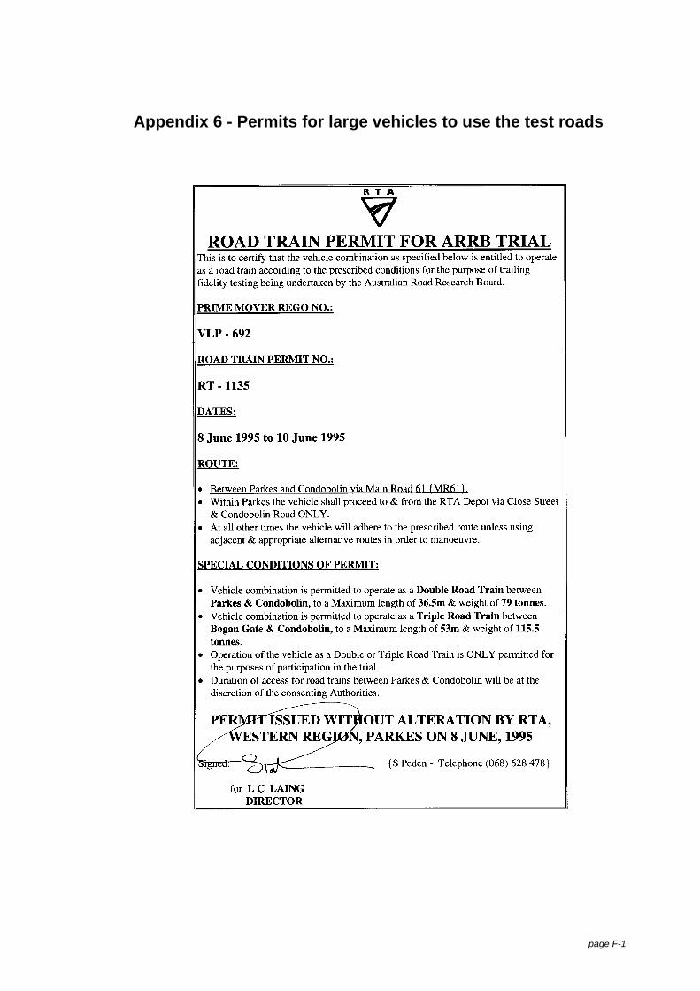
page F-1
Appendix 6 - Permits for large vehicles to use the test roads

page F-2

page F-3

page G-1
Appendix 7 - Sample data files
Annex 1 - Raw data FileThis sample below shows 0.4 seconds of data to demonstrate the file form. The file containsheader information and data in analogue-digital (A/D) format. The first 2 lines of the header arethe general test condition information, such as vehicle type, speed and test road. The next linesare the information assigned to each data channel, including the transducer calibration constantand units, their location on the test vehicle and a short description of the transducer (serialnumber) if appropriate. If the calibration was obtained from a regression analysis later then theconstant is set to 1. A negative sign is used to correct for the transducer orientation, eg. to allowan increase in chassis height to be positive. The next information in the header is the odocalibration constant, the data sampling frequency and date and time at the start of dataacquisition.
The first column of the data is the time increment for each record. The next 16 columns containthe data for each of the respective transducer channels and the last column is the odo count,summing odo pulses from the start of the logging session."Route access tests: - Vehicle: A123"Test conditions: 90 km/h - MBE"Channel 1 -0.1963 g/v Lateral Accelerometer: PM (s/n 205)"Channel 2 -18.1820 deg/sec/v Yaw rate gyro: PM"Channel 3 -0.2055 g/v Lateral Accelerometer: Rear Trailer (s/n 201)"Channel 4 -18.1820 deg/sec/v Yaw rate gyro: Rear Trailer"Channel 5 -0.2003 g/v Lateral Accelerometer: Front Trailer (s/n 896)"Channel 6 -0.1916 g/v Lateral Accelerometer Mid Trailer (s/n 902)"Channel 7 -1.0000 V/V Steer Wheel Angle: Driver Side"Channel 8 -1.0000 V/V Steer Wheel Angle: Passenger Side"Channel 9 -1.0000 mm/v Chassis Height: Passenger Side"Channel 10 -1.0000 mm/v Chassis Height: Driver Side"Channel 11 -1.0000 mm/v Rear Axle Motion: Passenger side"Channel 12 -1.0000 mm/v Rear Axle Motion: Driver side"Channel 13 -1.0000 V/V LPI 2 - Trailer 2"Channel 14 -1.0000 V/V LPI 3 - Rear Trailer"Channel 15 1.0000 V/V Dolly Articulation Angle"Channel 16 -1.0000 V/V LPI 1 - Prime Mover"Odo Cal 4260.000 p/km"Sampling 40 Hz"Start Time 15:10:06 Date 25/05/95
0.000 163 -223 230 4 -5 -7 -563 1091 461 325 291 735 0 874 0 1532 00.025 213 -41 188 -1 -4 -5 -558 1086 423 301 302 742 0 987 1 -531 60.050 230 -71 165 1 -6 -7 -564 1086 409 295 331 744 2 -696 -1 1590 90.075 148 -136 163 0 -4 -3 -564 1087 395 297 363 739 -1 973 0 1486 110.100 111 -183 175 -2 -7 -7 -563 1086 377 283 355 727 0 879 -1 1508 140.125 112 -160 172 0 -6 -7 -561 1087 369 272 311 707 0 -709 -2 1540 170.150 140 -123 152 -3 -5 -4 -561 1085 377 268 286 710 0 -578 -2 1492 190.175 156 -121 144 -3 -7 -6 -562 1088 387 270 295 711 -1 -599 -1 1504 220.200 64 -151 140 -4 -6 -9 -563 1087 419 283 309 706 0 -616 0 1491 240.225 0 -171 163 -4 -9 -8 -558 1087 446 297 311 699 0 -542 -2 1489 270.250 82 -157 175 -2 -4 -6 -557 1081 442 304 309 706 0 996 0 1512 300.275 185 -130 159 -5 -7 -5 -557 1083 414 306 321 720 0 925 -1 1520 320.300 180 -93 145 -4 -8 -8 -555 1087 402 313 330 714 0 854 0 -553 350.325 90 -82 145 -5 -7 -8 -560 1086 410 328 327 700 0 985 0 -546 380.350 47 -121 151 -2 -3 -7 -558 1089 415 329 308 692 -1 872 1 -559 400.375 95 -150 157 -2 -5 -6 -557 1086 419 326 285 698 0 998 0 -569 430.400 115 -131 156 -3 -4 -4 -555 1082 431 333 260 703 0 992 0 -577 45

page G-2
Annex 2 - Sample Comment fileFile: C:\Series I\f_mbe60.CMT
Elapsed time Time Odo Distance Speed Comment0.00 10:06:14 Start Time11.81 10:06:26 885 201 58 start
22.64 10:06:37 1692 385 66 shade
71.74 10:07:26 5352 1218 66 end
Logging Time = 75.6 sec
Mean speed = 61.1 km/h
Logging distance = 1283.3 m
Annex 3 - Sample Statistical Summary fileFile: C:\Series I\E_sae90.DAT64.119 sampling time (s)
Channel Mean SD RMS Max Min Range Skew Kurtosis
1 -0.023 0.097 0.100 0.231 -0.289 0.520 -0.044 -0.6132 2.431 0.796 2.558 5.416 -0.932 6.348 -0.151 0.4503 -0.047 0.022 0.052 0.025 -0.127 0.152 0.149 0.2134 -0.447 0.463 0.644 0.799 -2.397 3.196 -1.090 2.8915 -0.025 0.019 0.031 0.032 -0.079 0.111 0.175 -0.2246 0.003 0.001 0.003 0.005 0.001 0.004 -0.180 -0.4947 3.583 0.008 3.583 3.604 3.552 0.052 -0.982 0.6898 1.032 0.007 1.032 1.062 1.008 0.054 -0.188 0.1999 -48.950 11.600 50.310 -16.600 -85.940 69.340 -0.234 -0.131
10 75.900 11.130 76.710 111.300 33.200 78.130 0.042 -0.00911 -0.607 0.367 0.709 1.653 -1.624 3.277 0.773 1.55412 -2.948 0.365 2.971 -1.541 -4.998 3.457 -0.402 2.47213 0.875 2.041 2.221 2.664 -3.213 5.877 -0.915 -1.08214 2.571 2.773 3.781 4.846 -3.928 8.774 -1.307 -0.19215 -0.003 0.003 0.004 0.005 -0.012 0.017 0.408 -0.57316 -2.165 2.695 3.457 3.931 -4.170 8.101 0.962 -1.00417 25.2 1.2 27.8 24.6 3.2218 90.9 4.3 100.1 88.5 11.6
Channel 17 is vehicle forward velocity (m/s)Channel 18 is vehicle speed (km/h)

page G-3
Annex 4 - Sample lateral movement data file from the videoCALFILE=C:\VIDEOPC\DOUBLERT.CAL Mean 8.35A2MBE751.xls Std. Dev 62.39
Max 186.36Min -144.74
Range 331.10Kurtosis 0.154
Skewness 0.082
Time Screen co-ordinates Position(Uncorrected) (mm)
0.5 246 275 -14.56 87.871.0 227 281 -85.87 16.561.5 215 282 -130.96 -28.532.0 216 283 -127.16 -24.732.5 199 289 -190.82 -88.393.0 196 292 -201.96 -99.533.5 241 290 -33.00 69.434.0 236 288 -51.84 50.594.5 225 287 -93.20 9.235.0 236 292 -51.73 50.705.5 235 292 -55.49 46.946.0 236 296 -51.62 50.816.5 242 299 -29.02 73.417.0 245 300 -17.74 84.697.5 250 301 1.05 103.488.0 251 302 4.82 107.258.5 229 304 -77.67 24.769.0 222 357 -102.22 0.219.5 212 345 -139.95 -37.52
10.0 213 333 -136.64 -34.2110.5 223 332 -99.28 3.1511.0 222 332 -103.02 -0.5911.5 232 328 -65.73 36.7012.0 218 329 -118.08 -15.6512.5 217 329 -121.82 -19.3913.0 244 331 -20.76 81.6713.5 272 327 83.93 186.3614.0 268 322 68.89 171.3214.5 246 322 -13.49 88.9415.0 244 322 -20.98 81.4615.5 234 322 -58.42 44.0216.0 231 322 -69.65 32.7816.5 241 322 -32.21 70.2217.0 237 323 -47.16 55.2717.5 243 323 -24.70 77.7418.0 228 326 -80.76 21.6718.5 236 327 -50.79 51.6419.0 236 327 -50.79 51.6419.5 238 329 -43.26 59.1720.0 214 332 -132.94 -30.51

page H-1
Appendix 8 - Test vehicle dimensions and axle loads
Vehicle Dimensions
VehicleCode
Haulingunit
wheelbase
Trailer'S' dimension
Drawbarlength
Overalllength
(m)Lead Mid Rear Lead Rear
A 5.8 8.6 - - - - 18.4B 5.8 8.6 8.4 - 4.1 - 33.7C 5.8 8.6 8.4 8.6 4.1 4.1 49.0D 3.4 9.1 8.6 - - - 24.9E 3.8 8.3 7.2 - - - 22.9F 5.3 8.8 8.8 8.8 3.6 3.6 49.4G 5.3 8.6 8.5 - 5.2 - 33.4H 4.7 3.23 - - 4.6 - 17.2
Vehicle Axle loads
Vehicle Hauling unit Trailer Dolly GCMCode Steer Drive Lead Mid Rear Lead Rear (t)
A 5.8 16 20.5 - - - - 42.3B 5.8 16 20.5 20.5 - 15 - 77.7C 5.8 16 20.5 20.6 20.45 14.8 15 113.1D 5.6 14.9 21.2 19.2 - - - 60.8E 5.8 15.8 21.4 15.2 - - - 58.1F 6.5 11.7 12.7 12.6 10.9 9.1 9.2 72.7G 6.4 16.4 20.7 20.3 - 16.1 - 79.9H 6.1 16.5 11.0 - - 9.6 - 40.5

page I-1
Appendix 9 - Series I test vehicle dimensions
1500
575086008400
48990
1550
4500
31902550
41008550
300015003000 30001000
Vehicle 'C': (A123-T23-T23) A-triple (also units for Vehicles 'A' (A123) and 'B'(A123-T23))
13902900 1510
3400
90508640
2700
24900
Vehicle 'D': B-double - Steel Suspension (B1233)

page I-2
13502450 1050
3800
83257176
1225
22900
87709780
Vehicle 'E': B-double - Air Suspension (B1232)
1350
1300
5300
87508790
49400
1280 1200
3640
22902260
1250
34808795
1200 1250
Vehicle 'F': A-Triple, car carrier (A123-T22-T22)
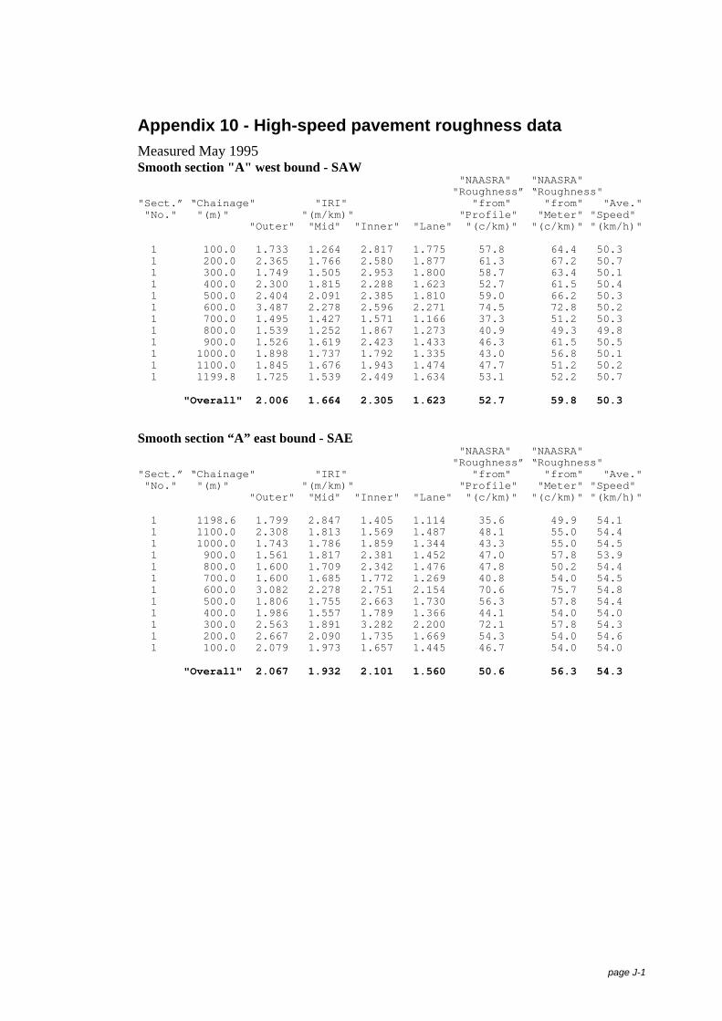
page J-1
Appendix 10 - High-speed pavement roughness dataMeasured May 1995Smooth section "A" west bound - SAW "NAASRA" "NAASRA" "Roughness” “Roughness""Sect.” “Chainage" "IRI" "from" "from" "Ave." "No." "(m)" "(m/km)" "Profile" "Meter" "Speed" "Outer" "Mid" "Inner" "Lane" "(c/km)" "(c/km)" "(km/h)"
1 100.0 1.733 1.264 2.817 1.775 57.8 64.4 50.3 1 200.0 2.365 1.766 2.580 1.877 61.3 67.2 50.7 1 300.0 1.749 1.505 2.953 1.800 58.7 63.4 50.1 1 400.0 2.300 1.815 2.288 1.623 52.7 61.5 50.4 1 500.0 2.404 2.091 2.385 1.810 59.0 66.2 50.3 1 600.0 3.487 2.278 2.596 2.271 74.5 72.8 50.2 1 700.0 1.495 1.427 1.571 1.166 37.3 51.2 50.3 1 800.0 1.539 1.252 1.867 1.273 40.9 49.3 49.8 1 900.0 1.526 1.619 2.423 1.433 46.3 61.5 50.5 1 1000.0 1.898 1.737 1.792 1.335 43.0 56.8 50.1 1 1100.0 1.845 1.676 1.943 1.474 47.7 51.2 50.2 1 1199.8 1.725 1.539 2.449 1.634 53.1 52.2 50.7
"Overall" 2.006 1.664 2.305 1.623 52.7 59.8 50.3
Smooth section “A” east bound - SAE "NAASRA" "NAASRA" "Roughness” “Roughness""Sect.” “Chainage" "IRI" "from" "from" "Ave." "No." "(m)" "(m/km)" "Profile" "Meter" "Speed" "Outer" "Mid" "Inner" "Lane" "(c/km)" "(c/km)" "(km/h)"
1 1198.6 1.799 2.847 1.405 1.114 35.6 49.9 54.1 1 1100.0 2.308 1.813 1.569 1.487 48.1 55.0 54.4 1 1000.0 1.743 1.786 1.859 1.344 43.3 55.0 54.5 1 900.0 1.561 1.817 2.381 1.452 47.0 57.8 53.9 1 800.0 1.600 1.709 2.342 1.476 47.8 50.2 54.4 1 700.0 1.600 1.685 1.772 1.269 40.8 54.0 54.5 1 600.0 3.082 2.278 2.751 2.154 70.6 75.7 54.8 1 500.0 1.806 1.755 2.663 1.730 56.3 57.8 54.4 1 400.0 1.986 1.557 1.789 1.366 44.1 54.0 54.0 1 300.0 2.563 1.891 3.282 2.200 72.1 57.8 54.3 1 200.0 2.667 2.090 1.735 1.669 54.3 54.0 54.6 1 100.0 2.079 1.973 1.657 1.445 46.7 54.0 54.0
"Overall" 2.067 1.932 2.101 1.560 50.6 56.3 54.3

page J-2
Smooth section “B” east bound - SBE "NAASRA" "NAASRA" "Roughness” “Roughness""Sect.” “Chainage" "IRI" "from" "from" "Ave." "No." "(m)" "(m/km)" "Profile" "Meter" "Speed" "Outer" "Mid" "Inner" "Lane" "(c/km)" "(c/km)" "(km/h)"
1 1798.4 1.597 1.505 2.591 1.530 49.6 52.9 56.9 1 1700.0 1.337 1.405 2.028 1.225 39.3 50.2 57.2 1 1600.0 1.479 1.376 1.815 1.235 39.6 45.5 57.6 1 1500.0 1.408 1.178 2.338 1.357 43.7 47.4 57.7 1 1400.0 1.751 1.161 1.847 1.314 42.3 48.4 57.5 1 1300.0 1.698 1.745 1.792 1.326 42.7 44.6 57.2 1 1200.0 1.812 1.689 2.117 1.247 40.0 55.9 57.4 1 1100.0 1.321 1.442 2.052 1.236 39.7 48.4 56.9 1 1000.0 1.643 1.547 1.673 1.154 36.9 49.3 57.0 1 900.0 1.633 1.595 1.828 1.321 42.5 45.5 57.5 1 800.0 1.809 1.292 1.463 1.266 40.7 44.6 57.6 1 700.0 1.645 1.526 1.743 1.286 41.4 49.3 57.8 1 600.0 1.296 1.802 1.345 .894 28.2 43.7 57.6 1 500.0 1.339 1.701 1.326 .974 30.9 40.8 57.2 1 400.0 1.743 1.361 1.436 1.143 36.6 42.7 56.9 1 300.0 1.828 1.480 1.336 1.121 35.8 48.4 57.5 1 200.0 1.620 1.407 1.334 1.027 32.6 46.5 57.2 1 100.0 1.430 1.465 1.181 .935 29.5 39.0 57.1
"Overall" 1.577 1.482 1.735 1.199 38.4 46.8 57.3
Rough section "B" west bound - SBW "NAASRA" "NAASRA" "Roughness” “Roughness""Sect.” “Chainage" "IRI" "from" "from" "Ave." "No." "(m)" "(m/km)" "Profile" "Meter" "Speed" "Outer" "Mid" "Inner" "Lane" "(c/km)" "(c/km)" "(km/h)"
1 100.0 1.338 1.444 2.108 1.301 41.9 50.2 50.7 1 200.0 1.412 1.701 2.511 1.482 48.0 44.6 50.4 1 300.0 1.388 1.373 1.674 1.131 36.1 43.7 50.3 1 400.0 1.370 1.535 1.786 1.132 36.2 47.4 50.3 1 500.0 1.905 1.451 2.931 1.917 62.6 57.8 50.3 1 600.0 1.630 1.395 2.322 1.435 46.4 55.9 49.7 1 700.0 1.604 1.819 2.673 1.605 52.1 58.7 50.2 1 800.0 1.314 1.724 1.347 .906 28.6 47.4 50.3 1 900.0 1.347 1.767 1.635 1.111 35.5 48.4 50.2 1 1000.0 1.501 1.633 1.464 1.004 31.9 52.1 50.5 1 1100.0 1.888 1.601 1.556 1.248 40.1 57.8 50.5 1 1200.0 1.572 1.994 1.717 1.256 40.3 55.9 49.9 1 1300.0 1.710 1.808 1.827 1.362 43.9 56.8 50.0 1 1400.0 1.752 1.326 1.376 1.198 38.4 53.1 49.9 1 1500.0 1.757 1.142 1.650 1.192 38.2 63.4 50.0 1 1600.0 1.783 1.285 2.644 1.725 56.1 54.0 49.9 1 1700.0 1.832 1.573 1.911 1.476 47.7 55.0 50.2 1 1796.8 1.815 1.775 1.697 1.252 40.2 54.6 50.5
"Overall" 1.606 1.575 1.935 1.318 42.5 53.1 50.2
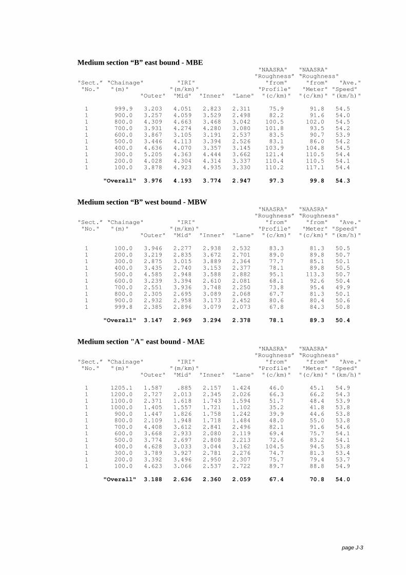
page J-3
Medium section “B” east bound - MBE "NAASRA" "NAASRA" "Roughness” “Roughness""Sect.” “Chainage" "IRI" "from" "from" "Ave." "No." "(m)" "(m/km)" "Profile" "Meter" "Speed" "Outer" "Mid" "Inner" "Lane" "(c/km)" "(c/km)" "(km/h)"
1 999.9 3.203 4.051 2.823 2.311 75.9 91.8 54.5 1 900.0 3.257 4.059 3.529 2.498 82.2 91.6 54.0 1 800.0 4.309 4.663 3.468 3.042 100.5 102.0 54.5 1 700.0 3.931 4.274 4.280 3.080 101.8 93.5 54.2 1 600.0 3.867 3.105 3.191 2.537 83.5 90.7 53.9 1 500.0 3.446 4.113 3.394 2.526 83.1 86.0 54.2 1 400.0 4.636 4.070 3.357 3.145 103.9 104.8 54.5 1 300.0 5.205 4.363 4.444 3.662 121.4 110.5 54.4 1 200.0 4.028 4.304 4.314 3.337 110.4 110.5 54.1 1 100.0 3.878 4.923 4.935 3.330 110.2 117.1 54.4
"Overall" 3.976 4.193 3.774 2.947 97.3 99.8 54.3
Medium section “B” west bound - MBW "NAASRA" "NAASRA" "Roughness” “Roughness""Sect.” “Chainage" "IRI" "from" "from" "Ave." "No." "(m)" "(m/km)" "Profile" "Meter" "Speed" "Outer" "Mid" "Inner" "Lane" "(c/km)" "(c/km)" "(km/h)"
1 100.0 3.946 2.277 2.938 2.532 83.3 81.3 50.5 1 200.0 3.219 2.835 3.672 2.701 89.0 89.8 50.7 1 300.0 2.875 3.015 3.889 2.364 77.7 85.1 50.1 1 400.0 3.435 2.740 3.153 2.377 78.1 89.8 50.5 1 500.0 4.585 2.948 3.588 2.882 95.1 113.3 50.7 1 600.0 3.239 3.394 2.610 2.081 68.1 92.6 50.4 1 700.0 2.551 3.936 3.748 2.250 73.8 95.4 49.9 1 800.0 2.305 2.695 3.089 2.068 67.7 81.3 50.1 1 900.0 2.932 2.958 3.173 2.452 80.6 80.4 50.6 1 999.8 2.385 2.896 3.079 2.073 67.8 84.3 50.8
"Overall" 3.147 2.969 3.294 2.378 78.1 89.3 50.4
Medium section "A" east bound - MAE "NAASRA" "NAASRA" "Roughness” “Roughness""Sect.” “Chainage" "IRI" "from" "from" "Ave." "No." "(m)" "(m/km)" "Profile" "Meter" "Speed" "Outer" "Mid" "Inner" "Lane" "(c/km)" "(c/km)" "(km/h)"
1 1205.1 1.587 .885 2.157 1.424 46.0 45.1 54.9 1 1200.0 2.727 2.013 2.345 2.026 66.3 66.2 54.3 1 1100.0 2.371 1.618 1.743 1.594 51.7 48.4 53.9 1 1000.0 1.405 1.557 1.721 1.102 35.2 41.8 53.8 1 900.0 1.447 1.826 1.758 1.242 39.9 44.6 53.8 1 800.0 2.109 1.948 1.718 1.484 48.0 55.0 53.8 1 700.0 4.408 3.612 2.841 2.496 82.1 91.6 54.6 1 600.0 3.668 2.933 2.080 2.119 69.4 75.7 54.1 1 500.0 3.774 2.697 2.808 2.213 72.6 83.2 54.1 1 400.0 4.628 3.033 3.044 3.162 104.5 94.5 53.8 1 300.0 3.789 3.927 2.781 2.276 74.7 81.3 53.4 1 200.0 3.392 3.496 2.950 2.307 75.7 79.4 53.7 1 100.0 4.623 3.066 2.537 2.722 89.7 88.8 54.9
"Overall" 3.188 2.636 2.360 2.059 67.4 70.8 54.0
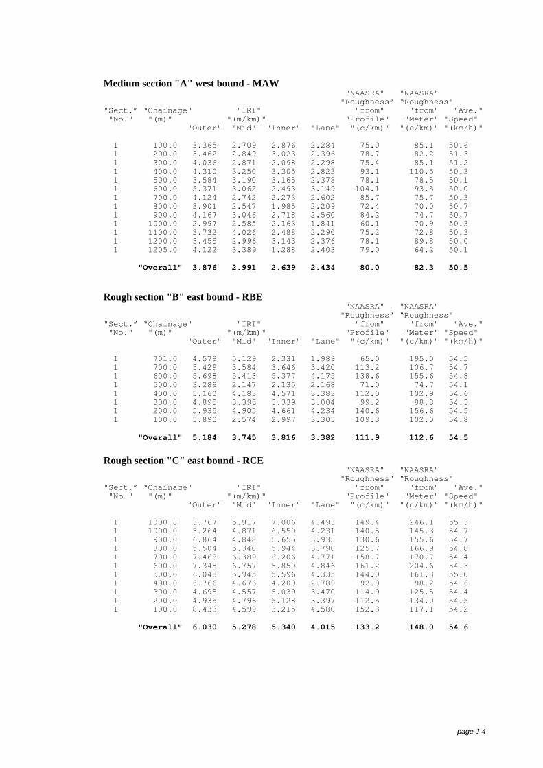
page J-4
Medium section "A" west bound - MAW "NAASRA" "NAASRA" "Roughness” “Roughness""Sect.” “Chainage" "IRI" "from" "from" "Ave." "No." "(m)" "(m/km)" "Profile" "Meter" "Speed" "Outer" "Mid" "Inner" "Lane" "(c/km)" "(c/km)" "(km/h)"
1 100.0 3.365 2.709 2.876 2.284 75.0 85.1 50.6 1 200.0 3.462 2.849 3.023 2.396 78.7 82.2 51.3 1 300.0 4.036 2.871 2.098 2.298 75.4 85.1 51.2 1 400.0 4.310 3.250 3.305 2.823 93.1 110.5 50.3 1 500.0 3.584 3.190 3.165 2.378 78.1 78.5 50.1 1 600.0 5.371 3.062 2.493 3.149 104.1 93.5 50.0 1 700.0 4.124 2.742 2.273 2.602 85.7 75.7 50.3 1 800.0 3.901 2.547 1.985 2.209 72.4 70.0 50.7 1 900.0 4.167 3.046 2.718 2.560 84.2 74.7 50.7 1 1000.0 2.997 2.585 2.163 1.841 60.1 70.9 50.3 1 1100.0 3.732 4.026 2.488 2.290 75.2 72.8 50.3 1 1200.0 3.455 2.996 3.143 2.376 78.1 89.8 50.0 1 1205.0 4.122 3.389 1.288 2.403 79.0 64.2 50.1
"Overall" 3.876 2.991 2.639 2.434 80.0 82.3 50.5
Rough section "B" east bound - RBE "NAASRA" "NAASRA" "Roughness” “Roughness""Sect.” “Chainage" "IRI" "from" "from" "Ave." "No." "(m)" "(m/km)" "Profile" "Meter" "Speed" "Outer" "Mid" "Inner" "Lane" "(c/km)" "(c/km)" "(km/h)"
1 701.0 4.579 5.129 2.331 1.989 65.0 195.0 54.5 1 700.0 5.429 3.584 3.646 3.420 113.2 106.7 54.7 1 600.0 5.698 5.413 5.377 4.175 138.6 155.6 54.8 1 500.0 3.289 2.147 2.135 2.168 71.0 74.7 54.1 1 400.0 5.160 4.183 4.571 3.383 112.0 102.9 54.6 1 300.0 4.895 3.395 3.339 3.004 99.2 88.8 54.3 1 200.0 5.935 4.905 4.661 4.234 140.6 156.6 54.5 1 100.0 5.890 2.574 2.997 3.305 109.3 102.0 54.8
"Overall" 5.184 3.745 3.816 3.382 111.9 112.6 54.5
Rough section "C" east bound - RCE "NAASRA" "NAASRA" "Roughness” “Roughness""Sect.” “Chainage" "IRI" "from" "from" "Ave." "No." "(m)" "(m/km)" "Profile" "Meter" "Speed" "Outer" "Mid" "Inner" "Lane" "(c/km)" "(c/km)" "(km/h)"
1 1000.8 3.767 5.917 7.006 4.493 149.4 246.1 55.3 1 1000.0 5.264 4.871 6.550 4.231 140.5 145.3 54.7 1 900.0 6.864 4.848 5.655 3.935 130.6 155.6 54.7 1 800.0 5.504 5.340 5.944 3.790 125.7 166.9 54.8 1 700.0 7.468 6.389 6.206 4.771 158.7 170.7 54.4 1 600.0 7.345 6.757 5.850 4.846 161.2 204.6 54.3 1 500.0 6.048 5.945 5.596 4.335 144.0 161.3 55.0 1 400.0 3.766 4.676 4.200 2.789 92.0 98.2 54.6 1 300.0 4.695 4.557 5.039 3.470 114.9 125.5 54.4 1 200.0 4.935 4.796 5.128 3.397 112.5 134.0 54.5 1 100.0 8.433 4.599 3.215 4.580 152.3 117.1 54.2
"Overall" 6.030 5.278 5.340 4.015 133.2 148.0 54.6

page J-5
Rough section "C" west bound - RCW "NAASRA" "NAASRA" "Roughness” “Roughness""Sect.” “Chainage" "IRI" "from" "from" "Ave." "No." "(m)" "(m/km)" "Profile" "Meter" "Speed" "Outer" "Mid" "Inner" "Lane" "(c/km)" "(c/km)" "(km/h)"
1 100.0 4.392 4.700 3.548 2.770 91.3 117.1 50.2 1 200.0 3.729 3.691 3.587 2.839 93.7 105.8 50.2 1 300.0 4.570 4.146 3.875 3.159 104.4 99.2 50.5 1 400.0 4.311 4.485 3.694 2.817 92.9 103.9 49.9 1 500.0 7.185 4.413 5.563 4.583 152.4 139.6 49.9 1 600.0 4.545 4.472 5.653 3.290 108.8 134.9 50.6 1 700.0 4.038 4.199 4.481 2.904 95.8 126.5 50.6 1 800.0 3.883 4.193 5.066 3.232 106.9 134.9 50.0 1 900.0 4.328 4.277 4.992 3.422 113.3 123.6 50.2 1 999.6 4.186 5.071 6.941 3.940 130.7 134.5 50.3
"Overall" 4.517 4.364 4.739 3.295 109.0 122.0 50.2
Rough section "B" west bound - RBW "NAASRA" "NAASRA" "Roughness” “Roughness""Sect.” “Chainage" "IRI" "from" "from" "Ave." "No." "(m)" "(m/km)" "Profile" "Meter" "Speed" "Outer" "Mid" "Inner" "Lane" "(c/km)" "(c/km)" "(km/h)"
1 100.0 4.178 3.673 2.629 2.663 87.7 87.9 50.6 1 200.0 6.412 4.175 4.871 4.523 150.4 154.7 50.6 1 300.0 5.254 3.960 5.107 3.795 125.8 118.0 50.4 1 400.0 5.175 3.699 4.624 3.963 131.5 118.9 50.0 1 500.0 3.338 2.724 3.772 2.558 84.2 92.6 50.7 1 600.0 6.313 5.602 6.228 4.743 157.8 163.2 50.1 1 700.0 6.093 3.730 3.297 3.434 113.7 118.0 50.6 1 700.7 1.108 2.242 1.271 .653 20.0 7.9 54.9
"Overall" 5.248 3.936 4.358 3.665 121.5 121.8 50.4
Rough section "A" west bound - RAW "NAASRA" "NAASRA" "Roughness” “Roughness""Sect.” “Chainage" "IRI" "from" "from" "Ave." "No." "(m)" "(m/km)" "Profile" "Meter" "Speed" "Outer" "Mid" "Inner" "Lane" "(c/km)" "(c/km)" "(km/h)"
1 100.0 5.745 3.353 3.214 3.607 119.5 99.2 57.2 1 200.0 7.070 5.199 4.596 4.176 138.7 106.7 56.9 1 300.0 6.931 4.820 4.696 4.383 145.6 161.3 57.1 1 400.0 6.256 3.107 4.218 3.903 129.5 118.0 56.9 1 500.0 7.102 5.677 5.862 4.981 165.8 139.6 56.9 1 600.0 6.994 3.436 3.395 3.832 127.1 100.1 57.3 1 700.0 6.041 3.126 3.770 3.767 124.9 116.1 56.7 1 799.9 6.368 3.266 3.751 3.871 128.4 106.8 57.2
"Overall" 6.564 3.998 4.188 4.065 134.9 118.5 57.0
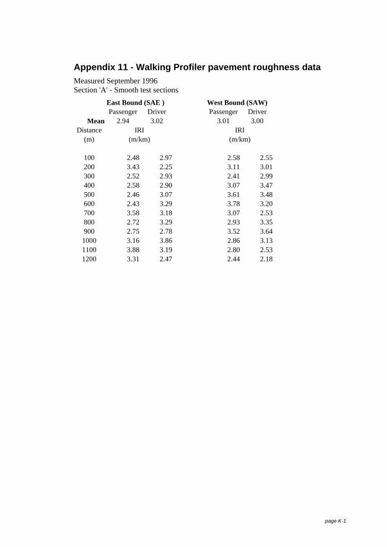
page K-1
Appendix 11 - Walking Profiler pavement roughness dataMeasured September 1996Section 'A' - Smooth test sections
East Bound (SAE ) West Bound (SAW)Passenger Driver Passenger Driver
Mean 2.94 3.02 3.01 3.00Distance IRI IRI
(m) (m/km) (m/km)
100 2.48 2.97 2.58 2.55200 3.43 2.25 3.11 3.01300 2.52 2.93 2.41 2.99400 2.58 2.90 3.07 3.47500 2.46 3.07 3.61 3.48600 2.43 3.29 3.78 3.20700 3.58 3.18 3.07 2.53800 2.72 3.29 2.93 3.35900 2.75 2.78 3.52 3.64
1000 3.16 3.86 2.86 3.131100 3.88 3.19 2.80 2.531200 3.31 2.47 2.44 2.18
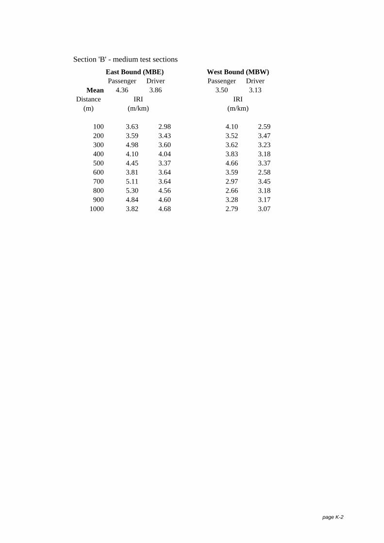
page K-2
Section 'B' - medium test sectionsEast Bound (MBE) West Bound (MBW)Passenger Driver Passenger Driver
Mean 4.36 3.86 3.50 3.13Distance IRI IRI
(m) (m/km) (m/km)
100 3.63 2.98 4.10 2.59200 3.59 3.43 3.52 3.47300 4.98 3.60 3.62 3.23400 4.10 4.04 3.83 3.18500 4.45 3.37 4.66 3.37600 3.81 3.64 3.59 2.58700 5.11 3.64 2.97 3.45800 5.30 4.56 2.66 3.18900 4.84 4.60 3.28 3.17
1000 3.82 4.68 2.79 3.07

page K-3
Section 'C' - Rough test sectionsEast Bound (RCW) West Bound (RCE)Passenger Driver Passenger Driver
Mean 4.39 4.52 5.90 5.18Distance IRI IRI
(m) (m/km) (m/km)
100 3.96 3.71 3.96 6.09200 4.25 3.91 4.25 5.47300 4.07 3.95 4.07 5.76400 4.38 3.74 4.38 5.60500 4.40 5.03 4.40 5.71600 6.27 5.29 6.27 5.60700 4.36 4.68 4.36 4.05800 3.77 4.76 3.77 4.87900 3.46 4.57 3.46 5.05
1000 4.92 5.51 4.92 3.59

page L-1
Appendix 12 - Summary of the pavement roughness data
The test roads used for this work were coded as follows:
Smooth, Medium or Rough, section 'A', 'B' or 'C' respectively for different sections withsimilar IRI values in either east or west bound direction.
Table L-1: Test road codes
Section Condition Direction of travel Code
A Smooth East SAE
A Smooth West SAW
B Medium East MBE
B Medium West MBW
C Rough East RCE
C Rough West RCW
The following Table is presented to provide a comparison of the road test section asmeasured by the two profile systems.
Table L-2: Comparison of roughness measurements for the test sections
Walking Profiler, September 96 Laser Profilometer, May 95Roughness Roughness
Section Length (IRI) (IRI)(m) Left Right Lane Left Right Lane
SAW 1,200 2.99 3.00 3.00 2.01 2.31 2.16
SAE 1,200 2.92 3.00 2.96 2.07 2.01 2.04
MBE 1,000 4.31 3.84 4.08 3.98 3.77 3.88
MBW 1,000 3.47 3.13 3.30 3.15 3.29 3.22
RCW 1,000 4.38 4.52 4.45 4.52 4.74 4.63
RCE 1,000 5.90 5.13 5.51 6.03 5.34 5.69

page M-1
Appendix 13 - Test roads profile characteristicsWheel path profiles
Measured wheel path profiles corrected for crossfall and detrended are presented forthree road surfaces used in this work. The profile data was detrended using Matlab,Little and Shure, (1993). This function removes the best 'straight line' linear trend fromthe data and effectively high-pass filters the profiles removing the very long wave-lengths.
The road surface crossfall information computed from the measured wheel path profilesis also presented.
-0.5
-0.4
-0.3
-0.2
-0.1
0.0
0.1
0 200 400 600 800 1,000 1,200
Distance (m)
Profile(m)
PassengerDriver
Figure M-1: SAE driver and passenger wheel path profiles
-0.15
-0.10
-0.05
0.00
0.05
0.10
0 200 400 600 800 1,000 1,200
Distance (m)
Profile(m)
PassengerDriver
Figure M-2: SAE driver and passenger wheel path profiles detrended
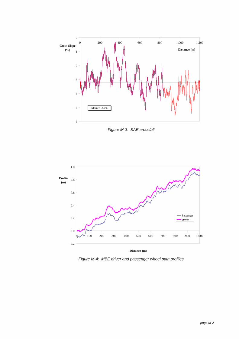
page M-2
-6
-5
-4
-3
-2
-1
00 200 400 600 800 1,000 1,200
Distance (m)Cross-Slope
(%)
Mean = -3.2%
Figure M-3: SAE crossfall
-0.2
0.0
0.2
0.4
0.6
0.8
1.0
0 100 200 300 400 500 600 700 800 900 1,000
Distance (m)
Profile(m)
PassengerDriver
Figure M-4: MBE driver and passenger wheel path profiles

page M-3
-0.15
-0.10
-0.05
0.00
0.05
0.10
0.15
0.20
0 100 200 300 400 500 600 700 800 900 1,000
Distance (m)
Profile(m)
PassengerDriver
Figure M-5: MBE driver and passenger wheel path profiles detrended
-9
-8
-7
-6
-5
-4
-3
-2
-1
00 200 400 600 800 1,000
Distance (m)Cross-Slope(%) Mean = -4.5%
Figure M-6: MBE crossfall

page M-4
-0.5
-0.4
-0.3
-0.2
-0.1
0.00 100 200 300 400 500 600 700 800 900 1,000
Distance (m)Profile
(m)
PassengerDriver
Figure M-7: RCW driver and passenger wheel path profiles
-0.15
-0.10
-0.05
0.00
0.05
0.10
0.15
0.20
0 100 200 300 400 500 600 700 800 900 1,000
Distance (m)
Profile(m)
PassengerDriver
Figure M-8: RCW driver and passenger wheel path detrended profiles

page M-5
-7
-6
-5
-4
-3
-2
-1
00 100 200 300 400 500 600 700 800 900 1,000
Distance (m)Cross-Slope
(%)
Mean = -4.0 %
Figure M-9: RCW crossfall
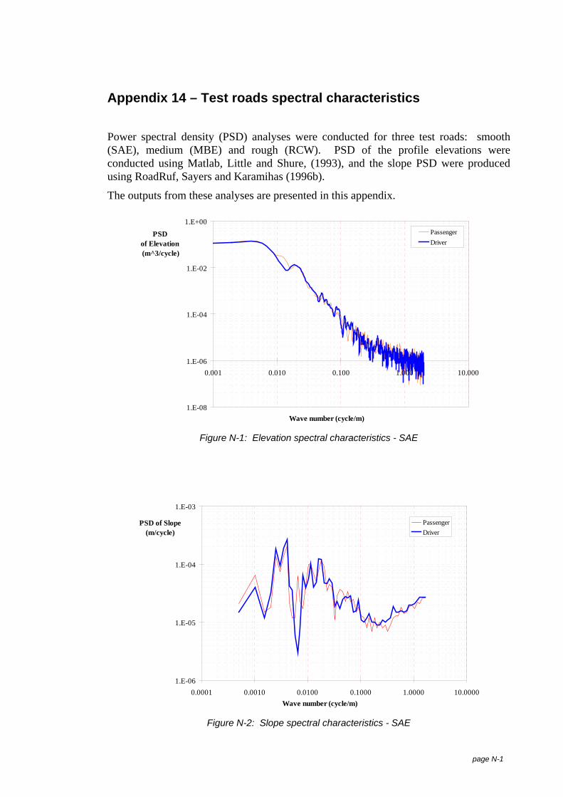
page N-1
Appendix 14 – Test roads spectral characteristics
Power spectral density (PSD) analyses were conducted for three test roads: smooth(SAE), medium (MBE) and rough (RCW). PSD of the profile elevations wereconducted using Matlab, Little and Shure, (1993), and the slope PSD were producedusing RoadRuf, Sayers and Karamihas (1996b).
The outputs from these analyses are presented in this appendix.
1.E-08
1.E-06
1.E-04
1.E-02
1.E+00
0.001 0.010 0.100 1.000 10.000
Wave number (cycle/m)
PSDof Elevation (m^3/cycle)
PassengerDriver
Figure N-1: Elevation spectral characteristics - SAE
1.E-06
1.E-05
1.E-04
1.E-03
0.0001 0.0010 0.0100 0.1000 1.0000 10.0000Wave number (cycle/m)
PSD of Slope(m/cycle)
PassengerDriver
Figure N-2: Slope spectral characteristics - SAE
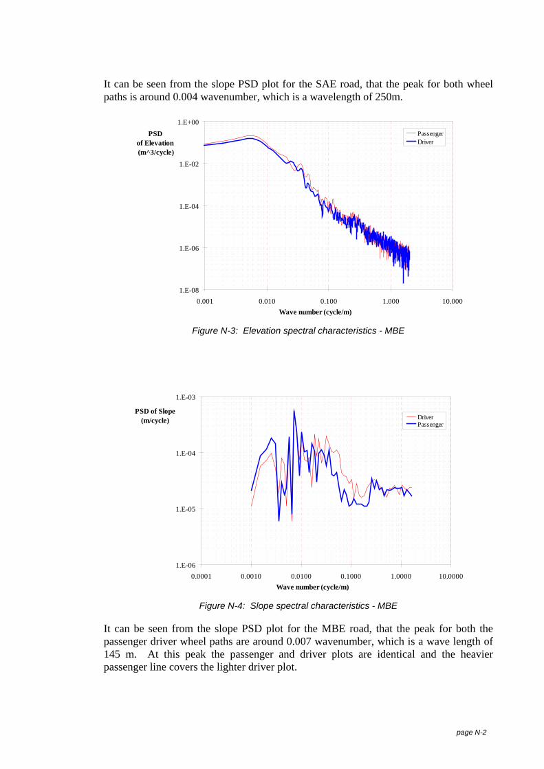
page N-2
It can be seen from the slope PSD plot for the SAE road, that the peak for both wheelpaths is around 0.004 wavenumber, which is a wavelength of 250m.
1.E-08
1.E-06
1.E-04
1.E-02
1.E+00
0.001 0.010 0.100 1.000 10.000Wave number (cycle/m)
PSDof Elevation (m^3/cycle)
PassengerDriver
Figure N-3: Elevation spectral characteristics - MBE
1.E-06
1.E-05
1.E-04
1.E-03
0.0001 0.0010 0.0100 0.1000 1.0000 10.0000Wave number (cycle/m)
PSD of Slope(m/cycle) Driver
Passenger
Figure N-4: Slope spectral characteristics - MBE
It can be seen from the slope PSD plot for the MBE road, that the peak for both thepassenger driver wheel paths are around 0.007 wavenumber, which is a wave length of145 m. At this peak the passenger and driver plots are identical and the heavierpassenger line covers the lighter driver plot.
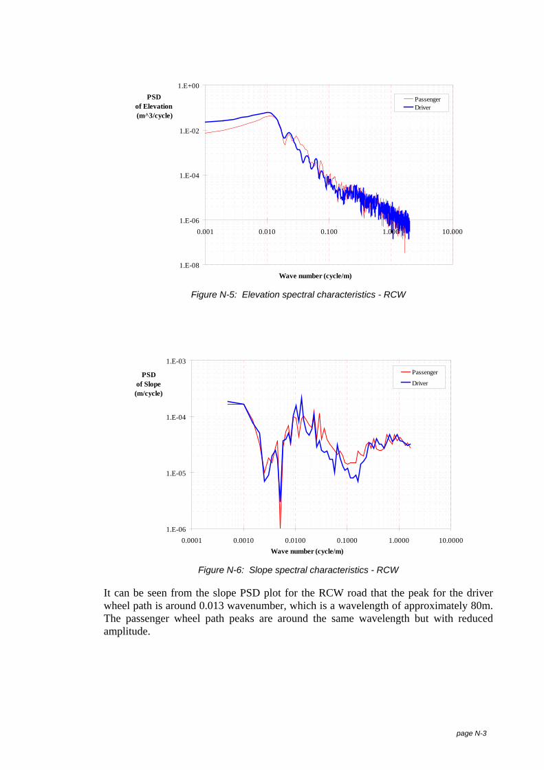
page N-3
1.E-08
1.E-06
1.E-04
1.E-02
1.E+00
0.001 0.010 0.100 1.000 10.000
Wave number (cycle/m)
PSDof Elevation (m^3/cycle)
PassengerDriver
Figure N-5: Elevation spectral characteristics - RCW
1.E-06
1.E-05
1.E-04
1.E-03
0.0001 0.0010 0.0100 0.1000 1.0000 10.0000Wave number (cycle/m)
PSDof Slope(m/cycle)
Passenger
Driver
Figure N-6: Slope spectral characteristics - RCW
It can be seen from the slope PSD plot for the RCW road that the peak for the driverwheel path is around 0.013 wavenumber, which is a wavelength of approximately 80m.The passenger wheel path peaks are around the same wavelength but with reducedamplitude.

page O-1
Appendix 15 – Computer Modelled vehicles, dimensions andaxle loads
Figure O-1: Single articulated (A123) dimensions and axle loads
Figure O-2: A-double (A123-T23) dimensions and axle loads

page O-2
Figure O-3: A-triple (A123-T23-T23) dimensions and axle loads
Figure O-4: B-double (B1233) dimensions and axle loads

page O-3
Figure O-5: B-triple (B12333) dimensions and axle loads
Figure O-6: Rigid-plus-three (R12-T23-T23-T23) dimensions and axle loads

page O-4
Figure O-7: Truck-trailer (R12-T12) dimensions and axle loads
(loaded to achieve a truck-trailer mass ratio of 1:1)
Figure O-8: Truck-trailer (R12-T22) dimensions and axle loads
(loaded to achieve a truck-trailer mass ratio of 1:1.22)

page P-1
Appendix 16 – Newspaper article on the field testing

Publications from this work
GEORGE. R.M., (1995). Trailing Fidelity of Articulated Vehicles - ARRB Transport Research,Preliminary Contract Report the Roads and Traffic Authority of New South Wales. No.RS 709D. (ARRB TR: Vermont South, Vic.
GEORGE, R.M., (1996a). Preliminary Report - Assessment of Combination Vehicles for Accessto the Road Network. ARRB Transport Research, Report N9501. (ARRB TR: VermontSouth, Vic.).
GEORGE, R.M., (1996b). Assessment of Combination Vehicles for Access to the RoadNetwork. Proc. Roads 96 Part 4 pp403-423. (ARRB TR: Vermont South, Vic.).
GEORGE, R.M., (1996c). Presentation at Swinburne Institute of Technology - The behaviourof large vehicles on rough surfaces.
GEORGE, R.M., (1997). Status Report - Road Network Access Standards for HeavyCommercial Vehicles. ARRB Transport Research, - phase II. CR OC6503. (ARRB TR:Vermont South, Vic.).
GEORGE, R.M., ELISCHER, M.P. and PREM. H. (1998c). Road Network Access Standardsfor Heavy Commercial Vehicles. Proc. 5th Int. Symp. on Commercial vehicle Weightsand Dimensions. (ARRB TR: Vermont South, Vic.).
GEORGE, R.M., ELISCHER, M.P. and PREM. H. (1998b) Exemption Guidelines for Non-Standard Vehicles. Proc. 5th Int. Symp. on Commercial vehicle Weights andDimensions. (ARRB TR: Vermont South, Vic.).