Towards High Performance Video Object Detection

Xizhou Zhu∗ Jifeng Dai Lu Yuan Yichen Wei

Microsoft Research Asia{v-xizzhu,jifdai,luyuan,yichenw}@microsoft.com

Abstract

There has been significant progresses for image objectdetection in recent years. Nevertheless, video object detec-tion has received little attention, although it is more chal-lenging and more important in practical scenarios.

Built upon the recent works [37, 36], this work proposesa unified approach based on the principle of multi-frameend-to-end learning of features and cross-frame motion.Our approach extends prior works with three new tech-niques and steadily pushes forward the performance enve-lope (speed-accuracy tradeoff), towards high performancevideo object detection.

1. IntroductionRecent years have witnessed significant progress in ob-

ject detection [17] in still images. However, directly apply-ing these detectors to videos faces new challenges. First,applying the deep networks on all video frames introducesunaffordable computational cost. Second, recognition ac-curacy suffers from deteriorated appearances in videos thatare seldom observed in still images, such as motion blur,video defocus, rare poses, etc.

There has been few works on video object detection. Therecent works [37, 36] suggest that principled multi-frameend-to-end learning is effective towards addressing abovechallenges. Specifically, data redundancy between consecu-tive frames is exploited in [37] to reduce the expensive fea-ture computation on most frames and improve the speed.Temporal feature aggregation is performed in [36] to im-prove the feature quality and recognition accuracy. Theseworks are the foundation of the ImageNet Video Object De-tection Challenge 2017 winner [6].

The two works focus on different aspects and presentstheir own drawbacks. Sparse feature propagation (seeEq. (1)) is used in [37] to save expensive feature compu-tation on most frames. Features on these frames are propa-

∗This work is done when Xizhou Zhu is intern at Microsoft ResearchAsia

gated from sparse key frames cheaply. The propagated fea-tures, however, are only approximated and error-prone, thushurting the recognition accuracy. Multi-frame dense featureaggregation (see Eq. (2)) is performed in [36] to improvefeature quality on all frames and detection accuracy as well.Nevertheless, it is much slower due to repeated motion es-timation, feature propagation and aggregation.

The two works are complementary in nature. They alsoshare the same principles: motion estimation module is builtinto the network architecture and end-to-end learning of allmodules is performed over multiple frames.

Built on these progresses and principles, this workpresents a unified approach that is faster, more accurate, andmore flexible. Specifically, three new techniques are pro-posed. First, sparsely recursive feature aggregation is usedto retain the feature quality from aggregation but as wellreduce the computational cost by operating only on sparsekey frames. This technique combines the merits of bothworks [37, 36] and performs better than both.

Second, spatially-adaptive partial feature updating is in-troduced to recompute features on non-key frames whereverpropagated features have bad quality. The feature quality islearnt via a novel formulation in the end-to-end training.This technique further improves the recognition accuracy.

Last, temporally-adaptive key frame scheduling replacesthe previous fixed key frame scheduling. It predicts the us-age of a key frame accordingly to the predicted feature qual-ity above. It makes the key frame usage more efficient.

The proposed techniques are unified with the priorworks [37, 36] under a unified viewpoint. Comprehensiveexperiments show that the three techniques steadily pushesforward the performance (speed-accuracy trade-off) enve-lope, towards high performance video object detection. Forexample, we achieve 77.8% mAP score at speed of 15.22frame per second. It establishes the new state-of-the-art.

2. From Image to Video Object Detection

Object detection in static images has achieved significantprogress in recent years using deep CNN [17]. State-of-the-art detectors share the similar methodology and network

arX

iv:1

711.

1157

7v1

[cs

.CV

] 3

0 N

ov 2

017

architecture, consisting of two conceptual steps.First step extracts a set of convolutional feature maps F

over the whole input image I via a fully convolutional back-bone network [31, 33, 14, 32, 34, 16, 2, 15, 35]. The back-bone network is usually pre-trained on the ImageNet clas-sification task and fine-tuned later. In this work, it is calledfeature network, Nfeat(I) = F . It is usually deep and slow.Computing it on all video frames is unaffordable.

Second step generates detection result y upon the featuremaps F , by performing region classification and boundingbox regression over either sparse object proposals [10, 13,9, 29, 4, 24, 12, 5] or dense sliding windows [26, 27, 28, 25],via a multi-branched sub-network. It is called detection net-work in this work, Ndet(F ) = y. It is randomly initializedand jointly trained with Nfeat. It is usually shallow and fast.

2.1. Revisiting Two Baseline Methods on Video

Sparse Feature Propagation [37]. It introduces the con-cept of key frame for video object detection, for the firsttime. The motivation is that similar appearance among adja-cent frames usually results in similar features. It is thereforeunnecessary to compute features on all frames.

During inference, the expensive feature network Nfeat isapplied only on sparse key frames (e.g., every 10th). Thefeature maps on any non-key frame i are propagated fromits preceding key frame k by per-pixel feature value warp-ing and bilinear interpolation. The between frame pixel-wise motion is recorded in a two dimensional motion fieldMi→k

1. The propagation from key frame k to frame i isdenoted as

Fk→i =W(Fk,Mi→k), (1)

whereW represents the feature warping function. Then thedetection network Ndet works on Fk→i, the approximationto the real feature Fi, instead of computing Fi from Nfeat.

The motion field is estimated by a lightweight flow net-work, Nflow(Ik, Ii) = Mi→k [7], which takes two framesIk, Ii as input. End-to-end training of all modules, in-cluding Nflow, greatly boosts the detection accuracy andmakes up for the inaccuracy caused by feature approxima-tion. Compared to the single frame detector, because thecomputation of Nflow and Eq. (1) is much cheaper (dozens,see Table 2 in [37]) than feature extraction in Nfeat, methodin [37] is much faster (up to 10×) with small accuracy drop(up to a few mAP points) (see, Figure 3 in [37]).

Dense Feature Aggregation [36]. It introduces the con-cept of temporal feature aggregation for video object detec-tion, for the first time. The motivation is that the deep fea-tures would be impaired by deteriorated appearance (e.g.,

1Since the warpingW from frame k to i adopts backward warping, wedirectly estimate and use backward motion field Mi→k for convenience.

motion blur, occlusion) on certain frames, but could be im-proved by aggregation from nearby frames.

During inference, feature network Nfeat is densely eval-uated on all frames. For any frame i, the feature mapsof all the frames within a temporal window [i − r, i + r](r = 2 ∼ 12 frames) are firstly warped onto the framei in the same way to [37] (see Eq. (1)), forming a set offeature maps {Fk→i|k ∈ [i − r, i + r]}. Different fromsparse feature propagation [37], the propagation occurs atevery frame instead of key frame only. In other words, everyframe is viewed as key frame.

The aggregated feature maps Fi at frame i is then ob-tained as the weighted average of all such feature maps,

Fi(p) =∑

k∈[i−r,i+r]

Wk→i(p) · Fk→i(p),∀p, (2)

where the weight Wk→i is adaptively computed as the sim-ilarity between the propagated feature maps Fk→i and thereal feature maps Fi. Instead, the feature F is projectedinto an embedding feature F e for similarity measure, andthe projection can be implemented by a tiny fully convolu-tional network (see Section 3.4 in [36]).

Wk→i(p) = exp

(F ek→i(p) · F e

i (p)

|F ek→i(p)| · |F e

i (p)|

),∀p. (3)

Note that both Eq. (2) and (3) are in a position-wise man-ner, as indicated by enumerating the location p. Theweight is normalized at every location p over nearby frames,∑

k∈[i−r,i+r]Wk→i(p) = 1.Similarly as [37], all modules including the flow net-

work and aggregation weight, etc., are jointly trained. Com-pared to the single frame detector, the aggregation in Eq. (2)greatly enhances the features and improves the detection ac-curacy (about 3 mAP points), especially for the fast movingobjects (about 6 mAP points) (see Table 1 in [36]). How-ever, runtime is about 3 times slower due to the repeatedflow estimation and feature aggregation over dense consec-utive frames.

3. High Performance Video Object Detection

The difference between the above two methods is appar-ent. [37] reduces feature computation by feature approx-imation, which decreases accuracy. [36] improves featurequality by adaptive aggregation, which increases computa-tion. They are naturally complementary.

On the other hand, they are based on the same twoprinciples: 1) motion estimation module is indispensablefor effective feature level communication between frames;2) end-to-end learning over multiple frames of all mod-ules is crucial for detection accuracy, as repeatedly verifiedin [37, 36].

flow-guidedfeature warping

feature aggregation

(a) Sparse Feature Propagation

(b) Dense Feature Aggregation

(c2) partially update featurefor non-key frames

(c1) recursively aggregate featurefor key frames

key frame

non-key frame

non-key framewith partial update

(c3) temporally-adaptivekey frame scheduling

pre-fixed key frame duration

all frames are key frames

………

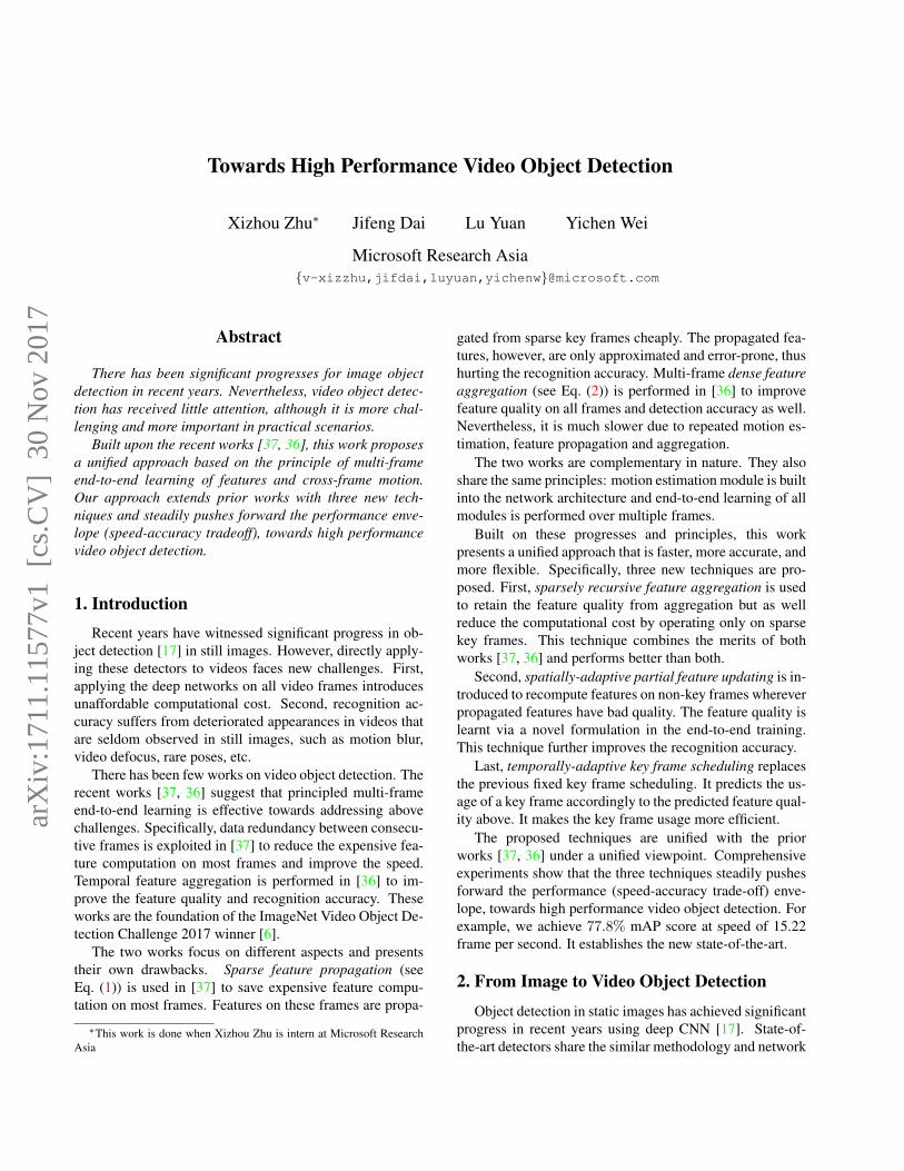
Figure 1. Illustration of the two baseline methods in [37, 36] andthree new techniques presented in Section 3.

Based on the same underlying principles, this paperpresents a common framework for high performance videoobject detection, as summarized in Section 3.4. It pro-poses three novel techniques. The first (Section 3.1) ex-ploits the complementary property and integrates the meth-ods in [37, 36]. It is both accurate and fast. The second(Section 3.2) extends the idea of adaptive feature computa-tion from temporal domain to spatial domain, resulting inspatially-adaptive feature computation that is more effec-tive. The third (Section 3.3) proposes adaptive key framescheduling that further improves the efficiency of featurecomputation.

These techniques are simple and intuitive. They natu-rally extend the previous works. Each one is built uponthe previous one(s) and steadily pushes forward the perfor-mance (runtime-accuracy trade off) envelope, as verified byextensive experiments in Section 5.

The two baseline methods and the three new techniquesare illustrated in Figure 1.

3.1. Sparsely Recursive Feature Aggregation

Although Dense Feature Aggregation [36] achieves sig-nificant improvement on detection accuracy, it is quite slow.On one hand, it densely evaluates feature network Nfeat onall frames, however that is unnecessary due to the similarappearance among adjacent frames. One the other hand,feature aggregation is performed on multiple feature mapsand thus multiple flow fields are needed to be estimated,

which largely slow down the detector.Here we propose Sparsely Recursive Feature Aggrega-

tion, which both evaluates feature networkNfeat and appliesrecursive feature aggregation only on sparse key frames.Given two succeeding key frames k and k′, the aggregatedfeature at frame k′ is computed by

Fk′ = Wk→k′ � Fk→k′ +Wk′→k′ � Fk′ , (4)

where Fk→k′ = W(Fk,Mk′→k), and � denotes element-wise multiplication. The weight is correspondingly normal-ized by Wk→k′(p) +Wk′→k′(p) = 1 at every location p.

This is a recursive version of Eq. (2), and the aggregationonly happens at sparse key frames. In principle, the aggre-gated key frame feature Fk aggregates the rich informationfrom all history key frames, and is then propagated to thenext key frame k′ for aggregating the original feature Fk′ .

3.2. Spatially-adaptive Partial Feature Updating

Although Sparse Feature Propagation [37] achieves re-markable speedup by approximating the real feature Fi, thepropagated feature map Fk→i is error-prone due to someparts with changing appearance among adjacent frames.

For non-key frames, we want to use the idea of featurepropagation for efficient computation, however Eq. (1) issubject to the quality of propagation. To quantify whetherthe propagated feature Fk→i is a good approximation of Fi,a feature temporal consistency Qk→i is introduced. We adda sibling branch on the flow network Nflow for predictingQk→i, together with motion field Mi→k, as

{Mi→k, Qk→i} = Nflow(Ik, Ii). (5)

If Qk→i(p) ≤ τ , the propagated feature Fk→i(p) is incon-sistent with the real feature Fi(p). That is to say, Fk→i(p)is a bad approximation, which suggests updating with realfeature Fi(p).

We consider a partial feature updating for non-keyframes. Feature at frame i is updated by

Fi = Uk→i �Nfeat(Ii) + (1− Uk→i)� Fk→i, (6)

where the updating mask Uk→i(p) = 1 if Qk→i(p) ≤ τ ,and Uk→i(p) = 0, otherwise. In our implementation, weadopt a more economic way which recomputes feature F (n)

i

of layer n from N (n)feat (F

(n−1)i ), where F (n−1)

i is the par-tially updated feature of layer n − 1. Thus the partial fea-ture updating can be calculated layer-by-layer. Consideringvaried resolution of feature maps in different layers, we usenearest neighbor interpolation for the updating mask.

Following [3], we use a straight-through estimator forthe gradient ∂Uk→i(p)

∂Qk→i(p)= −1, if |Qk→i(p) − τ | ≤ 1,

∂Uk→i(p)∂Qk→i(p)

= 0, otherwise. Thus it is fully differentiable.

We can regard Qk→i(p) − τ as a new valuable for the es-timation of Qk→i(p), since τ can be viewed as the bias ofQk→i(p), which takes no effect to the estimate Qk→i(p).For simplicity, we directly set τ = 0 in this paper.

To further improve the feature quality for non-keyframes, feature aggregation is also utilized as similar asEq. 4:

Fi = Wk→i � Fk→i +Wi→i � Fi, (7)

where the weight is normalized by Wk→i(p) +Wi→i(p) =1 at every location p.

3.3. Temporally-adaptive Key Frame Scheduling

Evaluating feature network Nfeat only on sparse keyframes is crucial for high speed. A naive key frame schedul-ing policy picks a key frame at a pre-fixed rate, e.g., every lframes[37]. A better key frame scheduling policy should beadaptive to the varying dynamics in the temporal domain. Itcan be designed based on the feature consistency indicatorQk→i:

key = is key(Qk→i). (8)

Here we designed a simple heuristic is key function:

is key(Qk→i) = [1

Np

∑p

1(Qk→i(p) ≤ τ)] > γ (9)

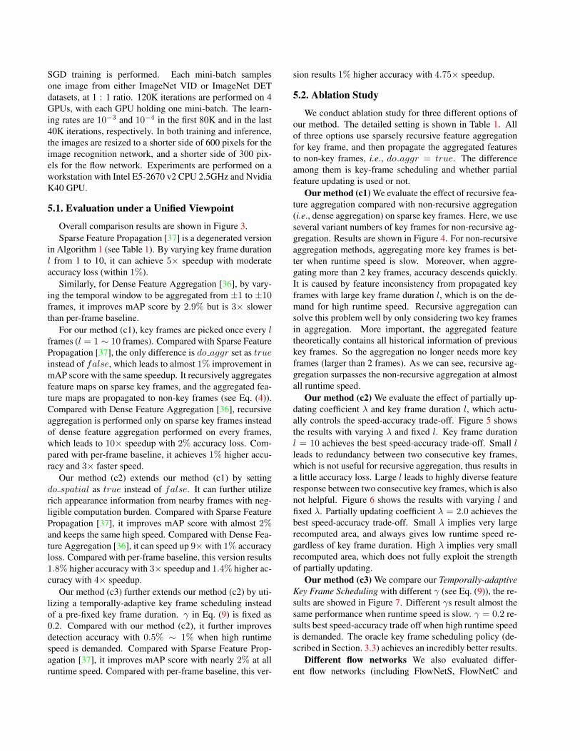
where 1(·) is the indicator function, Np is the number ofall locations p. For any location p, Qk→i(p) ≤ τ indi-cates changing appearance or large motion which will leadto bad feature propagation quality, if the area to recompute(Qk→i(p) ≤ τ ) is larger than a portion γ of all the pixels,the frame is marked as key. Figure. 2 shows an example ofthe area satisfiedQk→i(p) ≤ τ varying through time. Threeorange points are examples of key frame selected by ouris key function, their appearance are clearly different. Twoblue points are examples of non-key frame, their appear-ance indeed changed slightly compared with the precedingkey frame.

To explore the potential and upper bound of key framescheduling, we designed an oracle scheduling policy thatexploits the ground-truth information. The experiment isperformed with our proposed method, except for key framescheduling policy. Given any frame i, both the detectionresults of picking frame i as a key frame or non-key frameare computed, and the two mAP scores are also computedusing ground truth. If picking it as a key frame results ahigher mAP score, frame i is marked as key.

This oracle scheduling achieves a significantly better re-sult, i.e., 80.9% mAP score at 22.8 fps runtime speed. Thisindicates the importance of key frame scheduling and sug-gests that it is an important future working direction.

3.4. A Unified Viewpoint

All methods are summarized under a unified viewpoint.

To efficiently compute feature maps, Spatially-adaptivePartial Feature Updating (see Section 3.2) is utilized. Al-though Eq. (6) is only defined for non-key frames, it can begeneralized to all frames. Given a frame i and its precedingkey frame k, Eq. (6) is utilized, and summarized as

Fi = PartialUpdate(Ii, Fk,Mi→k, Qk→i). (10)

For key frames, Qk→i = −∞, propagated features Fk→i

are always bad approximation of real features Fi, we shouldrecompute feature Fi = Nfeat(Ii). For non-key frames,when Qk→i = +∞, propagated features Fk→i are al-ways good approximation of true features Fi, we directlyuse the propagated feature from the preceding key frameFi = Fk→i.

To enhance the partially updated feature maps Fi, fea-ture aggregation is utilized. Although Eq. (4) only definedSparsely Recursive Feature Aggregation for key frames, andEq. (7) only defined feature aggregation for partially up-dated non-key frames. Eq. (4) can be regarded as a de-generated version of Eq. (7), supposing i = k′, Fi = Fk′ .Thus feature aggregation is always performed as Eq. (7),and summarized as

Fi = G(Fk, Fi,Mi→k), (11)

To further improves the efficiency of feature computa-tion, Temporally-adaptive Key Frame Scheduling (see Sec-tion 3.3) is also utilized.

Inference Algorithm 1 summarizes the unified inferencealgorithm. Different settings result in different degeneratedversions, and Table 1 presents all methods from the unifiedviewpoint. Our method (c3) integrates all the techniquesand works best.

If Temporally-adaptive Key Frame Scheduling isadopted, and both options do aggr and do spatial areset as true, then it is the online version of our proposedmethod. Utilizing a naive key frame scheduling, i.e., pick akey every l frame, and both options do aggr and do spatialset as false, the algorithm degenerates to Sparse Fea-ture Propagation [37] when l > 1, and the per-framebaseline when l = 1. The algorithm would degenerateto Dense Feature Aggregation [36] under condition thatdo aggr = true, key = true, and do spatial = falsefor all the frames (i.e., l = 1), and the unified feature ag-gregation on Line 20 is replaced by the dense aggregationin Eq. (2). Among all options in Table 1, a sparse key framescheduling is crucial of fast inference, do aggr = true anddo spatial = true is crucial for high accuracy.

Training All the modules in the entire architecture canbe jointly trained. Due to memory limitation, in SGD, twonearby frames are randomly sampled in each mini-batch.

0 10 20 30 40 50 60 70 80 90 1000

0.05

0.1

0.15

0.2

0.25

0.3

0.35

frames

∑p1(Q

k→i(p)≤ τ)/N

p

Figure 2. The area satisfying Qk→i(p) ≤ τ on video frames, where the key frame scheduling in Eq. (9) is applied (γ = 0.2).

method is key(·, ·) key frame usage do aggr do spatial accuracy↔speedper-frame baseline (*) all frames N.A false false noneSparse Feature Propagation [37] every l frames sparse, 1 false false lDense Feature Aggregation [36] all frames dense, ≥ 1 true false #key framesour method (c1) every l frames sparse, recursive true false lour method (c2) every l frames sparse, recursive true true l, λour method (c3) temporally-adaptive sparse, recursive true true λ, γ

Table 1. All methods under a unified viewpoint.

The preceding frame is set as key, and the succeeding one isset as non-key, which are denoted as Ik and Ii, respectively.

In the forward pass, feature network Nfeat is applied onIk to obtain the feature maps Fk. Next, a flow networkNflow runs on the frames Ii, Ik to estimate the 2D flow fieldMi→k and the feature consistency indicatorQk→i. Partiallyupdated feature maps Fi is computed through Eq. (6), andthen the aggregated current feature maps Fi is calculatedthrough Eq. (7). Finally, the detection sub-network Ndet isapplied on Fi to produce the result yi. Loss function is de-fined as,

L = Ldet(yi) + λ∑p

Uk→i(p), (12)

where the updating mask Uk→i is defined in Eq. (6). Thefirst term is the loss function for object detection, followingthe multi-task loss in Faster R-CNN [29], which consistsof classification loss and bounding box regression loss to-gether. The second term enforces a constraint on the size ofareas to be recomputed, and λ controls the speed-accuracytrade off.

During training, we enforce that Uk→i = 0 and Uk→i =1 with 1/3 probability, respectively, to encourage good per-formance for both cases of propagating feature and recom-puting feature from scratch. For methods without using par-tial feature updating, training does not change and Qk→i

is simply ignored during inference. Thus, a unified singletraining strategy is used.

3.5. Network Architecture

We introduce the incarnation of different sub-networksin our proposed model.

Flow network. We use FlowNet [7] (“simple” version).It is pre-trained on the Flying Chairs dataset [7]. It is ap-plied on images of half resolution and has an output strideof 4. As the feature network has an output stride of 16(see below), the flow field is downscaled by half to matchthe resolution of the feature maps. An additional randomlyinitialized 3x3 convolution is added to predict the featurepropagability indicator, which shares feature with the lastconvolution of the FlowNet.

Feature network. We adopt the state-of-the-art ResNet-101 [14] as the feature network. The ResNet-101 model ispre-trained on ImageNet classification. We slightly modifythe nature of ResNet-101 for object detection. We removethe ending average pooling and the fc layer, and retain theconvolution layers. To increase the feature resolution, fol-lowing the practice in [1, 4], the effective stride of the lastblock is changed from 32 to 16. Specially, at the beginningof the last block (“conv5” for both ResNet-101), the strideis changed from 2 to 1. To retain the receptive field size, thedilation of the convolutional layers (with kernel size > 1)in the last block is set as 2. Finally, a randomly initialized3 × 3 convolution is applied on top to reduce the featuredimension to 1024.

Detection network. We use state-of-the-art R-FCN [4]and follow the design in [37]. On top of the 1024-d feature

Algorithm 1 The unified flow-based inference algorithmfor video object detection.

1: input: video frames {Ii}2: k = 0 . initialize key frame3: F0 = Nfeat(I0)4: y0 = Ndet(F0)5: if do aggr then6: F0 = F0

7: end if8: for i = 1 to∞ do9: {Mi→k, Qk→i} = Nflow(Ik, Ii) . evaluate flow network

10: key = is key(Qk→i) . key frame scheduling11: if key then12: Qk→i = −∞ . need computing feature from scratch13: else if do spatial then14: Qk→i unchanged . need partially updating15: else16: Qk→i = +∞ . suppose always good quality, propagate17: end if18: Fi = PartialUpdate(Ii, Fk,Mi→k, Qk→i) . partially

update19: if do aggr then20: Fi = G(Fk, Fi,Mi→k) . recursively aggregate21: yi = Ndet(Fi)22: else23: yi = Ndet(Fi)24: end if25: if key then . update the most recent key frame26: k = i27: end if28: end for29: output: detection results {yi}

maps, the RPN sub-network and the R-FCN sub-networkare applied, which connect to the first 512-d and the last512-d features respectively. 9 anchors (3 scales and 3 aspectratios) are utilized in RPN, and 300 proposals are producedon each image. The position-sensitive score maps in R-FCNare of 7× 7 groups.

4. Related Work

Speed/accuracy trade-offs in object detection. Assummarized in [17], speed/accuracy trade-off of modern de-tection systems can be achieved by using different featurenetworks [31, 33, 14, 32, 34, 16, 2, 15, 35] and detectionnetworks [10, 13, 9, 29, 4, 24, 12, 5, 26, 27, 28, 25], orvarying some critical parameters such as image resolution,box proposal number. PVANET [22] and YOLO [27] evendesign specific feature networks for fast object detection.By applying several techniques (e.g. batch normalization,high resolution classifier, fine-grained features and multi-scale training), YOLO9000 [28] achieves higher accuracymeanwhile keep the high speed.

Since our proposed method only considers how to com-

pute higher quality feature faster by using temporal infor-mation, and is not designed for any specific feature net-works and detection networks, such techniques are also suit-able for our proposed method.

Video object detection. Existing object detection meth-ods incorporating temporal information in video can be sep-arated into box-level methods [21, 20, 11, 23, 19, 8] andfeature-level methods [37, 36] (both are flow-based meth-ods and introduced in Section 2.1).

Box-level methods usually focus on how to improve de-tection accuracy considering temporary consistency withina tracklet. T-CNN [20, 21] first propagates predicted bound-ing boxes to neighboring frames according to pre-computedoptical flows, and then generates tubelets by applying track-ing algorithms. Boxes along each tubelet will be re-scoredbased on the tubelet classification result. Seq-NMS [11]constructs sequences along nearby high-confidence bound-ing boxes from consecutive frames. Boxes of the sequenceare re-scored to the average confidence, other boxes closeto this sequence are suppressed. MCMOT [23] formu-lates the post-processing as a multi-object tracking problem,and finally tracking confidence are used to re-score detec-tion confidence. TPN [19] first generates tubelet proposalsacross multiple frames (≤ 20 frames) instead of boundingbox proposals in a single frame, and then each tubelet pro-posal is classified into different classes by a LSTM basedclassifier. D&T [8] simultaneously outputs detection boxesand regression based tracking boxes with a single convolu-tional neural networks, and detection boxes are linked andre-scored based on tracking boxes.

Feature-level methods usually use optical flow to getpixel-to-pixel correspondence among nearby frames. Al-though feature-level methods are more principle and canfurther incorporate with box-level methods, they sufferfrom inaccurate optical flow. Still ImageNet VID 2017winner is powered by feature-level methods DFF [37] andFGFA [36]. Our proposed method is also a feature-levelmethod, which introduces Spatially-adaptive Partial Fea-ture Updating to fix the inaccurate feature propagationcaused by inaccurate optical flow.

5. ExperimentsImageNet VID dataset [30] is a prevalent large-scale

benchmark for video object detection. Following the pro-tocols in [20, 23], model training and evaluation are per-formed on the 3,862 video snippets from the training set andthe 555 snippets from the validation set, respectively. Thesnippets are fully annotated, and are at frame rates of 25 or30 fps in general. There are 30 object categories, which area subset of the categories in the ImageNet DET dataset.

During training, following [20, 23], both the ImageNetVID training set and the ImageNet DET training set (onlythe same 30 categories as in ImageNet VID) are utilized.

SGD training is performed. Each mini-batch samplesone image from either ImageNet VID or ImageNet DETdatasets, at 1 : 1 ratio. 120K iterations are performed on 4GPUs, with each GPU holding one mini-batch. The learn-ing rates are 10−3 and 10−4 in the first 80K and in the last40K iterations, respectively. In both training and inference,the images are resized to a shorter side of 600 pixels for theimage recognition network, and a shorter side of 300 pix-els for the flow network. Experiments are performed on aworkstation with Intel E5-2670 v2 CPU 2.5GHz and NvidiaK40 GPU.

5.1. Evaluation under a Unified Viewpoint

Overall comparison results are shown in Figure 3.Sparse Feature Propagation [37] is a degenerated version

in Algorithm 1 (see Table 1). By varying key frame durationl from 1 to 10, it can achieve 5× speedup with moderateaccuracy loss (within 1%).

Similarly, for Dense Feature Aggregation [36], by vary-ing the temporal window to be aggregated from ±1 to ±10frames, it improves mAP score by 2.9% but is 3× slowerthan per-frame baseline.

For our method (c1), key frames are picked once every lframes (l = 1 ∼ 10 frames). Compared with Sparse FeaturePropagation [37], the only difference is do aggr set as trueinstead of false, which leads to almost 1% improvement inmAP score with the same speedup. It recursively aggregatesfeature maps on sparse key frames, and the aggregated fea-ture maps are propagated to non-key frames (see Eq. (4)).Compared with Dense Feature Aggregation [36], recursiveaggregation is performed only on sparse key frames insteadof dense feature aggregation performed on every frames,which leads to 10× speedup with 2% accuracy loss. Com-pared with per-frame baseline, it achieves 1% higher accu-racy and 3× faster speed.

Our method (c2) extends our method (c1) by settingdo spatial as true instead of false. It can further utilizerich appearance information from nearby frames with neg-ligible computation burden. Compared with Sparse FeaturePropagation [37], it improves mAP score with almost 2%and keeps the same high speed. Compared with Dense Fea-ture Aggregation [36], it can speed up 9×with 1% accuracyloss. Compared with per-frame baseline, this version results1.8% higher accuracy with 3× speedup and 1.4% higher ac-curacy with 4× speedup.

Our method (c3) further extends our method (c2) by uti-lizing a temporally-adaptive key frame scheduling insteadof a pre-fixed key frame duration. γ in Eq. (9) is fixed as0.2. Compared with our method (c2), it further improvesdetection accuracy with 0.5% ∼ 1% when high runtimespeed is demanded. Compared with Sparse Feature Prop-agation [37], it improves mAP score with nearly 2% at allruntime speed. Compared with per-frame baseline, this ver-

sion results 1% higher accuracy with 4.75× speedup.

5.2. Ablation Study

We conduct ablation study for three different options ofour method. The detailed setting is shown in Table 1. Allof three options use sparsely recursive feature aggregationfor key frame, and then propagate the aggregated featuresto non-key frames, i.e., do aggr = true. The differenceamong them is key-frame scheduling and whether partialfeature updating is used or not.

Our method (c1) We evaluate the effect of recursive fea-ture aggregation compared with non-recursive aggregation(i.e., dense aggregation) on sparse key frames. Here, we useseveral variant numbers of key frames for non-recursive ag-gregation. Results are shown in Figure 4. For non-recursiveaggregation methods, aggregating more key frames is bet-ter when runtime speed is slow. Moreover, when aggre-gating more than 2 key frames, accuracy descends quickly.It is caused by feature inconsistency from propagated keyframes with large key frame duration l, which is on the de-mand for high runtime speed. Recursive aggregation cansolve this problem well by only considering two key framesin aggregation. More important, the aggregated featuretheoretically contains all historical information of previouskey frames. So the aggregation no longer needs more keyframes (larger than 2 frames). As we can see, recursive ag-gregation surpasses the non-recursive aggregation at almostall runtime speed.

Our method (c2) We evaluate the effect of partially up-dating coefficient λ and key frame duration l, which actu-ally controls the speed-accuracy trade-off. Figure 5 showsthe results with varying λ and fixed l. Key frame durationl = 10 achieves the best speed-accuracy trade-off. Small lleads to redundancy between two consecutive key frames,which is not useful for recursive aggregation, thus results ina little accuracy loss. Large l leads to highly diverse featureresponse between two consecutive key frames, which is alsonot helpful. Figure 6 shows the results with varying l andfixed λ. Partially updating coefficient λ = 2.0 achieves thebest speed-accuracy trade-off. Small λ implies very largerecomputed area, and always gives low runtime speed re-gardless of key frame duration. High λ implies very smallrecomputed area, which does not fully exploit the strengthof partially updating.

Our method (c3) We compare our Temporally-adaptiveKey Frame Scheduling with different γ (see Eq. (9)), the re-sults are showed in Figure 7. Different γs result almost thesame performance when runtime speed is slow. γ = 0.2 re-sults best speed-accuracy trade off when high runtime speedis demanded. The oracle key frame scheduling policy (de-scribed in Section. 3.3) achieves an incredibly better results.

Different flow networks We also evaluated differ-ent flow networks (including FlowNetS, FlowNetC and

0 2 4 6 8 10 12 14 16 18 2072

73

74

75

76

77

runtime speed (fps)

mA

P (

%)

Sparse Feature Propagation [36]Dense Feature Aggregation [35]our method (c1)our method (c2)our method (c3)

Figure 3. Speed-accuracy trade-off curves for methods in Table 1.

0 2 4 6 8 10 12 14 16 18 2072

73

74

75

76

runtime speed (fps)

mA

P (

%)

non−recursive aggregation (2 key frames)non−recursive aggregation (3 key frames)non−recursive aggregation (4 key frames)recursive aggregation

Figure 4. Speed-accuracy trade-off curves for our method (c1) andits non-recursive aggregation variants.

9 10 11 12 13 14 15 16 17 18 1974

74.5

75

75.5

76

runtime speed (fps)

mA

P (

%)

key frame duration = 6key frame duration = 8key frame duration = 10key frame duration = 12key frame duration = 14

Figure 5. Speed-accuracy trade-off curves for our method (c2), andeach curve shares a fixed key frame duration l.

FlowNet2 [18]) for our proposed method. Results areshowed in Figure. 8. FlowNetS results best speed-accuracytrade-off, this is because fast inference of flow network isthe key to speedup in our proposed method. With jointtraining, FlowNetS can achieve significantly better results,which is consistent with [37, 36].

Deformable R-FCN [5] We further replace the detectionsystem with Deformable R-FCN, which is slightly slowerthan the original R-FCN but much more accurate. Resultsare showed in Figure. 9. Our proposed method works well,and achieves 77.8% mAP score at 15.2 fps runtime speed,better than ImageNet VID 2017 winner (76.8% mAP scoreat 15.4 fps runtime speed [6]).

5.3. Comparison with State-of-the-art Methods

We further compared with several state-of-the-art meth-ods & systems for object detection from video, with re-ported results on ImageNet VID validation. It is worth men-tioning that different recognition networks, object detectors,and post processing techniques are utilized in different ap-proaches. Thus it is hard to draw a fair comparison.

9 10 11 12 13 14 15 16 17 18 1974

74.5

75

75.5

76

runtime speed (fps)

mA

P (

%)

λ = 0.25λ = 0.5λ = 1.0λ = 2.0λ = 4.0

Figure 6. Speed-accuracy trade-off curves for our method (c2), andeach curve shares a fixed partially updating coefficient λ.

5 10 15 20 2572

74

76

78

80

82

runtime speed (fps)

mA

P (

%)

γ = 0.1γ = 0.2γ = 0.3oracle scheduling policy

Figure 7. Speed-accuracy trade-off curves for our method (c3) withdifferent γ.

0 2 4 6 8 10 12 14 16 18 2068

70

72

74

76

runtime speed (fps)

mA

P (

%)

FlowNetS+ftFlowNetSFlowNetCFlowNet2

Figure 8. Speed-accuracy trade-off curves for our method (c1)with different flow networks. ‘FlowNetS+ft’ stands for FlowNetSjointly trained within our proposed method. Other flow networksare used without joint training.

0 2 4 6 8 10 12 14 16 18 2074

75

76

77

78

79

runtime speed (fps)

mA

P (

%)

Sparse Feature Propagation [36]Dense Feature Aggregation [35]our method (c1)our method (c2)our method (c3)

Figure 9. Speed-accuracy trade-off curves for all methods in Ta-ble 1 combined with Deformable R-FCN.

Table 2 presents the results. For our method, we re-ported results by picking two operational points on curve“our method (c3)” from Figure 9. The mAP score is 78.6%at a runtime of 13.0 / 8.6 fps on Titan X / K40. The mAPscore slightly decrease to 77.8% at a faster runtime of 22.9/ 15.2 fps on Titan X / K40. As a comparison, TPN [19]gets an mAP score of 68.4% at a runtime of 2.1 fps on TitanX. In the latest paper of D&T [8], an mAP score of 75.8%

method feature network mAP (%)runtime (fps)(TitanX/K40)

Ours ResNet-101+DCN78.6 13.0 / 8.677.8 22.9 / 15.2

TPN [19] GoogLeNet 68.4 2.1 / -

D&T [8] ResNet-101 75.8 7.8 / -ImageNet VID2017 winner [6]

ResNet-101 76.8 - / 15.4

Table 2. Comparison with state-of-the-art methods.

is obtained at a runtime of 7.8 fps on Titan X. SequenceNMS [11] can be applied to D&T to further improve theperformance, which can also be applied in our approach.We also compared with the winning entry [6] of ImageNetVID challenge 2017, which is also based on sparse featurepropagation [37] and dense feature aggregation [36]. It getsan mAP score of 76.8% at a runtime of 15.4 fps on Titan X.It is heavily-engineered and the implementation details areunreported. Our method is more principled, and achievesbetter performance in terms of both accuracy and speed.

References[1] L.-C. Chen, G. Papandreou, I. Kokkinos, K. Murphy, and

A. L. Yuille. Semantic image segmentation with deep con-volutional nets and fully connected crfs. In ICLR, 2015. 5

[2] F. Chollet. Xception: Deep learning with depthwise separa-ble convolutions. In CVPR, 2017. 2, 6

[3] M. Courbariaux, I. Hubara, D. Soudry, R. El-Yaniv, andY. Bengio. Binarized neural networks: Training deep neu-ral networks with weights and activations constrained to +1or -1. arXiv preprint arXiv:1602.02830, 2016. 3

[4] J. Dai, Y. Li, K. He, and J. Sun. R-fcn: Object detection viaregion-based fully convolutional networks. In NIPS, 2016.2, 5, 6

[5] J. Dai, H. Qi, Y. Xiong, Y. Li, G. Zhang, H. Hu, and Y. Wei.Deformable convolutional networks. In ICCV, 2017. 2, 6, 8

[6] J. Deng, Y. Zhou, B. Yu, Z. Chen, S. Zafeiriou,and D. Tao. Speed/accuracytradeoffs forobjectdetection-fromvideo. http://image-net.org/challenges/talks_2017/Imagenet2017VID.pdf, 2017. 1, 8, 9

[7] A. Dosovitskiy, P. Fischer, E. Ilg, P. Hausser, C. Hazirbas,V. Golkov, P. v.d. Smagt, D. Cremers, and T. Brox. Flownet:Learning optical flow with convolutional networks. In ICCV,2015. 2, 5

[8] C. Feichtenhofer, A. Pinz, and A. Zisserman. Detect to trackand track to detect. In ICCV, 2017. 6, 9

[9] R. Girshick. Fast r-cnn. In ICCV, 2015. 2, 6[10] R. Girshick, J. Donahue, T. Darrell, and J. Malik. Rich fea-

ture hierarchies for accurate object detection and semanticsegmentation. In CVPR, 2014. 2, 6

[11] W. Han, P. Khorrami, T. Le Paine, P. Ramachandran,M. Babaeizadeh, H. Shi, J. Li, S. Yan, and T. S. Huang.

Seq-nms for video object detection. arXiv preprintarXiv:1602.08465, 2016. 6, 9

[12] K. He, G. Gkioxari, P. Dollar, and R. Girshick. Mask r-cnn.In ICCV, 2017. 2, 6

[13] K. He, X. Zhang, S. Ren, and J. Sun. Spatial pyramid poolingin deep convolutional networks for visual recognition. InECCV, 2014. 2, 6

[14] K. He, X. Zhang, S. Ren, and J. Sun. Deep residual learningfor image recognition. In CVPR, 2016. 2, 5, 6

[15] A. G. Howard, M. Zhu, B. Chen, D. Kalenichenko, W. Wang,T. Weyand, M. Andreetto, and H. Adam. Mobilenets: Effi-cient convolutional neural networks for mobile vision appli-cations. arXiv preprint arXiv:1704.04861, 2017. 2, 6

[16] G. Huang, Z. Liu, K. Q. Weinberger, and L. van der Maaten.Densely connected convolutional networks. In CVPR, 2017.2, 6

[17] J. Huang, V. Rathod, C. Sun, M. Zhu, A. Korattikara,A. Fathi, I. Fischer, Z. Wojna, Y. Song, S. Guadarrama, et al.Speed/accuracy trade-offs for modern convolutional objectdetectors. In CVPR, 2017. 1, 6

[18] E. Ilg, N. Mayer, T. Saikia, M. Keuper, A. Dosovitskiy, andT. Brox. Flownet 2.0: Evolution of optical flow estimationwith deep networks. In CVPR, 2017. 8

[19] K. Kang, H. Li, T. Xiao, W. Ouyang, J. Yan, X. Liu, andX. Wang. Object detection in videos with tubelet proposalnetworks. In CVPR, 2017. 6, 9

[20] K. Kang, H. Li, J. Yan, X. Zeng, B. Yang, T. Xiao, C. Zhang,Z. Wang, R. Wang, X. Wang, and W. Ouyang. T-cnn:Tubelets with convolutional neural networks for object de-tection from videos. arXiv preprint arxiv:1604.02532, 2016.6, 7

[21] K. Kang, W. Ouyang, H. Li, and X. Wang. Object detectionfrom video tubelets with convolutional neural networks. InCVPR, 2016. 6

[22] K.-H. Kim, S. Hong, B. Roh, Y. Cheon, and M. Park. Pvanet:Deep but lightweight neural networks for real-time object de-tection. arXiv preprint arXiv:1608.08021, 2016. 6

[23] B. Lee, E. Erdenee, S. Jin, M. Y. Nam, Y. G. Jung, and P. K.Rhee. Multi-class multi-object tracking using changing pointdetection. In ECCV, 2016. 6, 7

[24] T.-Y. Lin, P. Dollar, R. Girshick, K. He, B. Hariharan, andS. Belongie. Feature pyramid networks for object detection.In CVPR, 2017. 2, 6

[25] T.-Y. Lin, P. Goyal, R. Girshick, K. He, and P. Dollar.Focal loss for dense object detection. arXiv preprintarXiv:1708.02002, 2017. 2, 6

[26] W. Liu, D. Anguelov, D. Erhan, C. Szegedy, S. Reed, C.-Y.Fu, and A. C. Berg. Ssd: Single shot multibox detector. InECCV, 2016. 2, 6

[27] J. Redmon, S. Divvala, R. Girshick, and A. Farhadi. Youonly look once: Unified, real-time object detection. InCVPR, 2016. 2, 6

[28] J. Redmon and A. Farhadi. Yolo9000: better, faster, stronger.arXiv preprint arXiv:1612.08242, 2016. 2, 6

[29] S. Ren, K. He, R. Girshick, and J. Sun. Faster r-cnn: Towardsreal-time object detection with region proposal networks. InNIPS, 2015. 2, 5, 6

[30] O. Russakovsky, J. Deng, H. Su, J. Krause, S. Satheesh,S. Ma, Z. Huang, A. Karpathy, A. Khosla, M. Bernstein,A. Berg, and F.-F. Li. Imagenet large scale visual recognitionchallenge. In IJCV, 2015. 6

[31] K. Simonyan and A. Zisserman. Very deep convolutionalnetworks for large-scale image recognition. In ICLR, 2015.2, 6

[32] C. Szegedy, S. Ioffe, V. Vanhoucke, and A. Alemi. Inception-v4, inception-resnet and the impact of residual connectionson learning. arXiv preprint arXiv:1602.07261, 2016. 2, 6

[33] C. Szegedy, W. Liu, Y. Jia, P. Sermanet, S. Reed,D. Anguelov, D. Erhan, V. Vanhoucke, and A. Rabinovich.Going deeper with convolutions. In CVPR, 2015. 2, 6

[34] S. Xie, R. Girshick, P. Dollar, Z. Tu, and K. He. Aggregatedresidual transformations for deep neural networks. In CVPR,2017. 2, 6

[35] X. Zhang, X. Zhou, M. Lin, and J. Sun. Shufflenet: Anextremely efficient convolutional neural network for mobiledevices. arXiv preprint arXiv:1707.01083, 2017. 2, 6

[36] X. Zhu, Y. Wang, J. Dai, L. Yuan, and Y. Wei. Flow-guidedfeature aggregation for video object detection. In ICCV,2017. 1, 2, 3, 4, 5, 6, 7, 8, 9

[37] X. Zhu, Y. Xiong, J. Dai, L. Yuan, and Y. Wei. Deep featureflow for video recognition. In CVPR, 2017. 1, 2, 3, 4, 5, 6,7, 8, 9