Towards Climate Based Early Warning and Response Systems for Malaria

Maquins Odhiambo Sewe

Department of Public Health and Clinical Medicine

Epidemiology and Global Health

Umeå University, Sweden 2017

Responsible publisher under Swedish law: the Dean of the Medical Faculty

This work is protected by the Swedish Copyright Legislation (Act 1960:729)

ISBN: 978-91-7601-641-1

ISSN: 0346-6612

Electronic version available at http://umu.diva-portal.org/

Tryck/Printed by: UmU Print Service, Umeå UniversityUmeå, 2017

I dedicate this dissertation to my parents

“The future never takes care of itself; it is taken care of, shaped, molded, and

colored by the present. Our todays are what our yesterdays made them; our

tomorrows must inevitably be the product of our todays.” ~Dennis Kimbro

i

Table of Contents

Table of Contents i Abstract iii Abbreviations v Contributing Papers vii Preface ix Introduction 1

Malaria and how its transmitted 1 Malaria burden 4 Risk factors for malaria transmission 9 Malaria surveillance 15 Malaria early warning and detection 16 Evaluating economic benefit of early warning systems 17 Summary 20 Objectives 21

Materials and methods 22 Study setting 22 Verbal autopsy 24 Hospital surveillance 25 Environmental data 26 Statistical analysis 29 Methodologies paper by paper 33

Results 41 Distribution of malaria health outcomes 41 Distribution of weather variables 41 Seasonality of malaria deaths and environmental variables 44 Relationship between environmental factors and malaria mortality 46 Prediction of monthly malaria admissions 53 A framework for economic evaluation of early warning and response system

benefits 56 Discussion 60 Conclusions 71 Acknowledgements 72 References 74

ii

iii

Abstract

Background: Great strides have been made in combating malaria, however, the

indicators in sub Saharan Africa still do not show promise for elimination in the

near future as malaria infections still result in high morbidity and mortality

among children. The abundance of the malaria-transmitting mosquito vectors in

these regions are driven by climate suitability. In order to achieve malaria

elimination by 2030, strengthening of surveillance systems have been advocated.

Based on malaria surveillance and climate monitoring, forecasting models may

be developed for early warnings. Therefore, in this thesis, we strived to illustrate

the use malaria surveillance and climate data for policy and decision making by

assessing the association between weather variability (from ground and remote

sensing sources) and malaria mortality, and by building malaria admission

forecasting models. We further propose an economic framework for integrating

forecasts into operational surveillance system for evidence based decision-

making and resource allocation.

Methods: The studies were based in Asembo, Gem and Karemo areas of the

KEMRI/CDC Health and Demographic Surveillance System in Western Kenya.

Lagged association of rainfall and temperature with malaria mortality was

modeled using general additive models, while distributed lag non-linear models

were used to explore relationship between remote sensing variables, land surface

temperature(LST), normalized difference vegetation index(NDVI) and rainfall

on weekly malaria mortality. General additive models, with and without

boosting, were used to develop malaria admissions forecasting models for lead

times one to three months. We developed a framework for incorporating forecast

output into economic evaluation of response strategies at different lead times

including uncertainties. The forecast output could either be an alert based on a

threshold, or absolute predicted cases. In both situations, interventions at each

lead time could be evaluated by the derived net benefit function and uncertainty

incorporated by simulation.

Results: We found that the environmental factors correlated with malaria

mortality with varying latencies. In the first paper, where we used ground

weather data, the effect of mean temperature was significant from lag of 9 weeks,

with risks higher for mean temperatures above 25C. The effect of cumulative

precipitation was delayed and began from 5 weeks. Weekly total rainfall of more

than 120 mm resulted in increased risk for mortality. In the second paper, using

remotely sensed data, the effect of precipitation was consistent in the three areas,

with increasing effect with weekly total rainfall of over 40 mm, and then declined

at 80 mm of weekly rainfall. NDVI below 0.4 increased the risk of malaria

mortality, while day LST above 35C increased the risk of malaria mortality with

shorter lags for high LST weeks. The lag effect of precipitation was more delayed

iv

for precipitation values below 20 mm starting at week 5 while shorter lag effect

for higher precipitation weeks. The effect of higher NDVI values above 0.4 were

more delayed and protective while shorter lag effect for NDVI below 0.4. For all

the lead times, in the malaria admissions forecasting modelling in the third

paper, the boosted regression models provided better prediction accuracy. The

economic framework in the fourth paper presented a probability function of the

net benefit of response measures, where the best response at particular lead time

corresponded to the one with the highest probability, and absolute value, of a net

benefit surplus.

Conclusion: We have shown that lagged relationship between environmental

variables and malaria health outcomes follow the expected biological

mechanism, where presentation of cases follow the onset of specific weather

conditions and climate variability. This relationship guided the development of

predictive models showcased with the malaria admissions model. Further, we

developed an economic framework connecting the forecasts to response

measures in situations with considerable uncertainties. Thus, the thesis work has

contributed to several important components of early warning systems including

risk assessment; utilizing surveillance data for prediction; and a method to

identifying cost-effective response strategies. We recommend economic

evaluation becomes standard in implementation of early warning system to

guide long-term sustainability of such health protection programs.

Key words: Malaria, Mosquito, Lead time, Early Warnings, Forecasts,

Economic Evaluation, Rainfall, KEMRI/CDC HDSS, Kenya, Temperature, LST,

NDVI, Climate, HDSS, GAM, GAMBOOST, DLNM, Remote Sensing, Net

Benefit, Cost-Effectiveness, Boosting Regression, Weather, Public Health,

Infectious Diseases

v

Abbreviations

AS- AQ Artesunate – Amodiaquine

ACF Autocorrelation Function

ACT Artemisinin Combination Based Therapy

An. Anopheles

AR Autoregressive Term

AVHRR Advanced Very High Resolution Radiometer

CDC Centre for Disease Control

DDT Dichlorodiphenyltrichloroethane

DLM Distributed Lag Models

DLNM Distributed Lag Non-Linear Models

EIP Extrinsic Incubation Period

ETA Evapotranspiration

EVI Enhanced Vegetation Index

GAM General Additive Model

GAMLSS General Additive Models for Location, Scale and Shape

HDF-EOS Hierarchical Data Format- Earth Observing System

HDSS Health and Demographic Surveillance System

INDEPTH International Network for The Demographic Evaluation of

Populations and Their Health

InterVA Interpreting Vas

IPTp Intermittent Preventive Treatment for Pregnant Women

ITN Insecticide Treated Nets

KEMRI Kenya Medical Research Institute

KIMS Kenyan Malaria Indicator Survey

LLINs Long Lasting Insecticidal Nets

LST Land Surface Temperature

MAE Mean Absolute Error

MCMC Markov Chain Monte Carlo

MEW Malaria Early Warning System

MODIS Moderate Resolution Imaging Spectro-Radiometer

MVC Maximum Value Compositing

NASA National Aeronautics and Space Administration

NASDA National Space Development Space Agency of Japan

NDVI Normalized Difference Vegetation Index

NMAE Normalized Mean Absolute Error

NMCP National Malaria Control Program

NMSE Normalized Mean Squared Error

NN Nearest Neighbour

NOAA National Oceanic and Atmospheric Administration

P. falciparum Plasmodium falciparum

PACF Partial Autocorrelation Function

vi

pfPR P. falciparum prevalence rate

PSA Probability Sensitivity Analysis

RH Relative Humidity

RMSE Root Mean Squared Error

SP Sulfadoxine/Pyrimethamineÿ

TRMM Tropical Rainfall Measuring Mission

VA Verbal Autopsy

VI Vegetation Index

WHO World Health Organization

WMO World Meteorological Association

vii

Contributing Papers

This thesis is based on the papers I-IV. The papers I and II were published in

open access journals so no permission was required to reprint.

I. Sewe, M., Rocklöv, J., Williamson, J., Hamel, M., Nyaguara, A.,

Odhiambo, F., & Laserson, K. (2015). The association of weather

variability and under five malaria mortality in KEMRI/CDC HDSS in

Western Kenya 2003 to 2008: a time series analysis. Int J Environ

Res Public Health, 12(2), 1983-1997. doi:10.3390/ijerph120201983

II. Sewe, M. O., Ahlm, C., & Rocklöv, J. (2016). Remotely Sensed

Environmental Conditions and Malaria Mortality in Three Malaria

Endemic Regions in Western Kenya. PLoS One, 11(4), e0154204.

doi:10.1371/journal.pone.0154204

III. Sewe, M. O., Tozan, Y., Ahlm, C., & Rocklöv, J. (Submitted). Using

remote sensing environmental data to forecast malaria incidence at a

rural district hospital in Western Kenya.

IV. Sewe, M. O., Tozan, Y., Ahlm, C., & Rocklöv, J. (Manuscript). A

methodological framework for economic evaluation of operational

response to vector-borne disease forecasts.

viii

ix

Preface

The control and prevention of malaria is very important in countries in Sub-

Saharan Africa where malaria contributes to high levels of morbidity and

mortality. Children under the age of five are the most vulnerable with most of

the mortality occurring in this age group. Great progress has been observed in

taming the scourge of malaria, but in countries with higher prevalence the

progress has not been as expected and thus malaria still contributes to high

child mortality plunging communities affected to great suffering and

economic burden. In malaria prevalent areas, reducing malaria deaths in

children would yield huge gains in reducing the overall under five mortality

rates. The world health assembly in 2015, through the sustainable

development goals framework, has targeted the elimination of malaria in

countries reporting malaria transmission by 2030. The new set of sustainable

development goals continues and replaces the millennium development goals

that ended in 2015. To achieve the goal of elimination, improved malaria

surveillance technologies has been cited as one of the key strategies.

In Kenya, about 40% of the population is at risk of malaria. Endemic malaria

transmission is concentrated around the Lake Victoria region and part of the

coastal regions, while highland and semi-arid regions only occasionally

experience epidemics. The use of interventions in the control of malaria can

have great impact if they are implemented in a timely manner before

epidemics, or before anomalous increase in the cases beyond the seasonal

mean occurs. To have enough time to implement interventions, the routine

monitoring of malaria cases reported through active surveillance can provide

information regarding seasonal changes and epidemic anomalies in disease

transmission and provide a foundation for forecasting forthcoming

transmission in communities.

Malaria surveillance used in conjunction with environmental monitoring can

provide early warning alerts if aberrations are observed in comparison to

seasonal transmission patterns. WHO have advised the use of early warning

for the control of epidemics. Early detection using thresholds derived from

malaria surveillance, risk assessment and predictive models, form part of

malaria early warning system. In this thesis, we contribute to informing on the

feasibility and strategies to the development of a malaria early warning system

in an endemic region that is part of an ongoing health and demographic

surveillance system in Western Kenya. We do this, by assessing temporal

lagged risk associations between ground weather data as well as remotely

sensed data to malaria mortality. We use the information from the risk

assessment studies to develop early warning prediction models comparing

x

different lead times to single out the predictive skill and uncertainty. Alerts

emanating from early warning systems often fail to be utilized by decision

makers to initiate response actions due to the inherent possibility of false

alarms, and the lack of technical and strategic response capacity. To aid

decision makers on the timing of appropriate actions, we propose an economic

evaluation framework that integrates response actions with disease forecasts

and able to handle uncertainty in the prediction and response.

1

Introduction

Malaria and how its transmitted

Malaria parasite development in human host

Malaria infections occur when human blood is infected by protozoan parasite

called sporozoites of the genus Plasmodium which is transmitted by female

Anopheles mosquitoes when they take a blood meal from a host [1]. The

sporozoites invade the hepatocytes and proliferate into merozoites. Some

sporozoites differentiate into hypnozoites that remain in the liver for months

to years before dividing and developing into merozoites. It takes around six

days for P. falciparum sporozoites to develop into 40,000 merozoites per liver

cell. Malaria infection begins when the merozoites invade the erythrocytes [2].

A summary of the life cycle of malaria parasite in the human host is displayed

in Figure 1. It has been postulated that the malaria parasites originated from

gorillas [3].

There are five main malaria parasites namely P. vivax, P. malariae, P. ovale

and P. falciparum and more recently discovered P. knowlesi [4]. Currently P.

falciparum and P. vivax are the mostly encountered malaria parasites with P.

falciparum accounting for over 79% of the malaria parasites in East African

countries in Sub-Saharan Africa. P. falciparum malaria is responsible for high

morbidity and mortality in younger children below five years and responsible

for episodes of severe malaria in children [5, 6].

P. ovale has very limited distribution. P. falciparum malaria is characterized

as “subtertian, malignant persistent fevers”. Malaria infections are

characterized with febrile episodes, paroxysm with chills, rigors and sweating.

Malaria shares similar symptoms with other febrile illnesses, which include

body aches, headache, nausea, general weakness and prostration. This has

resulted in treatment of most febrile cases for which not all maybe malaria

related with antimalarial in countries such as Kenya [5].

2

Figure 1. Malaria parasite life cycle, (source: [7])

Malaria parasite development in mosquito

When the mosquito vector takes a blood meal from a human host it ingests

gametocytes which triggers the formation of gametes in the mosquito’s midgut

lumen [8]. In a process called exflagellation, the male microgametes fertilize

the female macrogametes to form a ‘zygote’. Temperature and PH levels of the

xanthurenic acid influence the rate of ‘zygote’ development. After the ‘zygotes’

are formed, meiosis happens and genetic recombination occurs. The spherical

‘zygote’ transforms into an ookinete. The ookinetes uses motility to leave the

blood meal bolus to penetrate the peritrophic matrix that encloses the blood

meal after which it penetrates the apical end of the mosquito midgut

epithelium [8]. The ookinete then transforms into oocysts, a process that takes

about 10-12 days and subsequently develops into sporozoites that burst into

the hemocoel. The sporozoites are then carried by circulation of haemolymph

to all tissues of the mosquito and eventually to the salivary glands [8].

Mosquito life cycle

Mosquitoes go through four distinct stages during their life. The stages are

egg, larva, pupa and adult as shown in Figure 2. The first three stages occur in

water while the adult is an active flying insect. Only the female mosquito bites

and feeds on bloods from humans or animals. After the female mosquito

3

obtains a blood meal, she lays the eggs directly on or near water. The eggs

hatch in water and mosquito larva or “wriggler emerges”. The development

of larva depends on temperature, type of mosquito and availability of food.

The larva lives in the water, feeds and develops into pupa or “tumbler”. The

pupa also lives in water but does not feed. Finally, the mosquito emerges from

the pupal case after 2 - 7 days in the pupal stage. The life cycle takes about two

weeks but depending on environmental conditions, it can take from 4 days to

1 month. The adult mosquito emerges onto the surface of the water and flies

away.

Figure 2. Mosquito development cycle (source: http://www.mosquito.org/life-cycle)

Malaria endemicity

There are three levels of malaria transmission zones. In areas with stable

endemic transmission, populations are continuously exposed to malaria

inoculations due to mosquito bites, however, with seasonal fluctuations. Due

to this persistent exposure, the population usually gets immunity from ages 4

to 5 years. The others are unstable endemic malaria and epidemic malaria

zones [1]. In unstable endemic malaria transmission setting, there is less

permanent transmissions and a huge fluctuation in transmission over time.

This affects immunity as individuals can be exposed to inoculations ranging

from intervals of one year to several years. Epidemic malaria is an extreme

form of unstable malaria where populations or groups of individuals are

subjected to an increase in transmission, not previously or normally

experienced. P. falciparum malaria epidemics usually results in very high

morbidity and mortality [1].

4

Malaria burden

Global burden

World Health Organization’s(WHO) 2015 world malaria report confirms that

concerted efforts towards the prevention and control of malaria has resulted

in significant gains in reducing global malaria burden. Since the year 2000, 57

countries have achieved millennium development goal 6C of over 75%

reduction in incidence while 18 countries achieved reduction of between 50-

75% in incidence by 2015 [9]. However, malaria endemic countries in Sub-

Saharan African, contributing over 88% in global malaria disease burden,

have registered below average decline, blamed on the weak health systems.

For example, Nigeria and Democratic Republic of Congo characterized as very

high stable endemic malaria transmission areas, with a parasite prevalence of

over 40%, together contributed 35% of the global estimated malaria deaths

[10]. Malaria still poses a major burden in most parts of the world with an

estimated 3.2 billion people at risk of infection [9].

European countries reported no malaria infections in 2015 while Southeast

Asia contributed 10% to the global incidence. By 2015, of the 106 WHO

countries, 33 registered less than 1000 malaria cases in 2015, suggesting that

most countries are progressing towards elimination [9].In 2000, 262 million

infections were reported compared to 214 million in 2015, resulting in an

overall decline of 18% over the 14-year period. In the same period malaria

incidence decreased by 37% with parasite prevalence among children 2 to 10

years decreasing from 33% in 2000 to 16% in 2015 [9].

In the same period, malaria deaths for all age groups declined by 48% from

839,000 in 2000 to 438,000 in 2015 and for children under five years, the

mortality reduced by 50% from 723,000 deaths in 2000 to 360,000 deaths in

2015. The WHO African region, which contributes to 90% of malaria deaths

in just 15 countries, registered 57% reduction in malaria mortality among

children from 694,000 in 2000 to 292,000 deaths in 2015. These reductions

represents huge gains in combating malaria contributing significantly towards

the achievement of millennium development goal 4 [9]. Overall, factoring in

changes in population, malaria mortality rate declined by 60% between 2000

and 2015, with a 66% reduction in African region for all ages and a 71%

reduction among children under five years [9].With the reductions achieved

in mortality, malaria was no longer the leading cause of mortality in children

in Africa having been relegated to position 4 contributing 10% to the mortality

burden in that age group and $900 million dollars saved through prevention

strategies over the 14 years [9].

5

Some challenges have been cited in relation to the fight to eliminate malaria

worldwide. As such are the report that 269 million of the 834 million people

at risk are not sleeping under mosquito nets, weaknesses in health systems,

insecticide resistance and anti-malaria drug resistance [9].

Malaria burden in Kenya

In Kenya 75% of the population, live in malaria prone regions. P. falciparum

is the major malaria Plasmodium parasite prevalent in Kenya. The malaria

risk in Kenya is not homogenous, the endemic lake region and coastal areas

are leading in malaria prevalence, and the children under five and pregnant

women at greatest risk due to low immunity [11]. A map of estimated malaria

prevalence for Kenya is shown in Figure 3. Over 50% of the households in the

country at risk of malaria use ITNs. Artesunate (AS)- Amodiaquine (AQ) is the

first-line medical treatment for malaria [9].

Figure 3. Map of Kenya showing spatial distribution of PfPR2-10. CE = Central province; CO =

Coastal province; EA = Eastern province; NA = Nairobi province; NE = North Eastern province;

NY = Nyanza province; RV = Rift Valley province; and WE = Western province. (Source: [12])

6

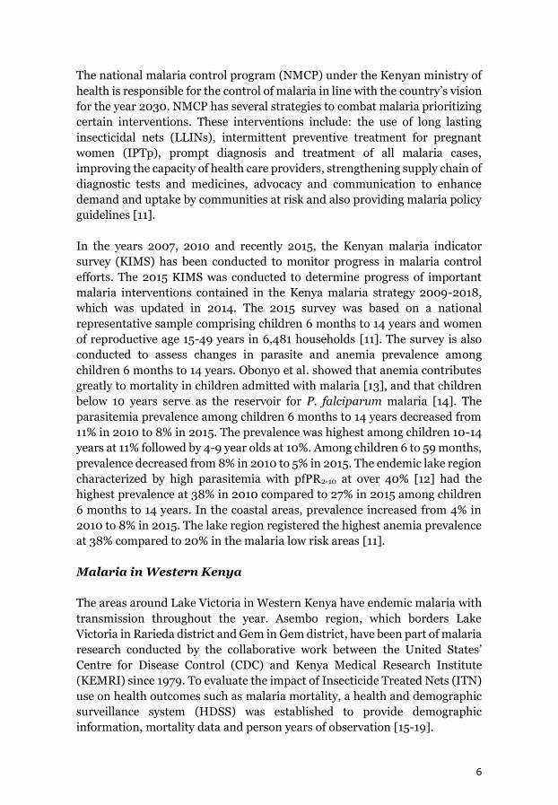
The national malaria control program (NMCP) under the Kenyan ministry of

health is responsible for the control of malaria in line with the country’s vision

for the year 2030. NMCP has several strategies to combat malaria prioritizing

certain interventions. These interventions include: the use of long lasting

insecticidal nets (LLINs), intermittent preventive treatment for pregnant

women (IPTp), prompt diagnosis and treatment of all malaria cases,

improving the capacity of health care providers, strengthening supply chain of

diagnostic tests and medicines, advocacy and communication to enhance

demand and uptake by communities at risk and also providing malaria policy

guidelines [11].

In the years 2007, 2010 and recently 2015, the Kenyan malaria indicator

survey (KIMS) has been conducted to monitor progress in malaria control

efforts. The 2015 KIMS was conducted to determine progress of important

malaria interventions contained in the Kenya malaria strategy 2009-2018,

which was updated in 2014. The 2015 survey was based on a national

representative sample comprising children 6 months to 14 years and women

of reproductive age 15-49 years in 6,481 households [11]. The survey is also

conducted to assess changes in parasite and anemia prevalence among

children 6 months to 14 years. Obonyo et al. showed that anemia contributes

greatly to mortality in children admitted with malaria [13], and that children

below 10 years serve as the reservoir for P. falciparum malaria [14]. The

parasitemia prevalence among children 6 months to 14 years decreased from

11% in 2010 to 8% in 2015. The prevalence was highest among children 10-14

years at 11% followed by 4-9 year olds at 10%. Among children 6 to 59 months,

prevalence decreased from 8% in 2010 to 5% in 2015. The endemic lake region

characterized by high parasitemia with pfPR2-10 at over 40% [12] had the

highest prevalence at 38% in 2010 compared to 27% in 2015 among children

6 months to 14 years. In the coastal areas, prevalence increased from 4% in

2010 to 8% in 2015. The lake region registered the highest anemia prevalence

at 38% compared to 20% in the malaria low risk areas [11].

Malaria in Western Kenya

The areas around Lake Victoria in Western Kenya have endemic malaria with

transmission throughout the year. Asembo region, which borders Lake

Victoria in Rarieda district and Gem in Gem district, have been part of malaria

research conducted by the collaborative work between the United States’

Centre for Disease Control (CDC) and Kenya Medical Research Institute

(KEMRI) since 1979. To evaluate the impact of Insecticide Treated Nets (ITN)

use on health outcomes such as malaria mortality, a health and demographic

surveillance system (HDSS) was established to provide demographic

information, mortality data and person years of observation [15-19].

7

In 2001, the HDSS was revitalized to monitor socio-demographic changes,

first in Asembo and then expanding to Gem in 2002 [20]. Adazu et al.

presented the mortality profile for the demographic study area for the year

2002 just after the HDSS had been started. They found that the under-five

mortality ratio was 227 per 1000 live births, and malaria contributed 75% of

all sick visits at the health facilities. Malaria and anemia were the main cause

of death in children 1 month to 11 years with mortality fractions of 28.9% and

19.8%, respectively [20]. The main anopheles vector was An. gambiae

constituting 95.6% of all mosquitoes collected between 2002 and 2003 with

7.2 infectious bites per person [20]. In the period 2002 to 2004 in the study

area, Amek et al. reported the prevalence of An. gambiae mosquitoes species

at 86% with entomological inoculation rates of 6.7, 9.3 and 9.6 infectious bites

per year for years 2002 to 2004 [21]. An. gambiae has been the dominant

Anopheles vector in the study area, but since the 2005, its population has

declined due to high ITN use. The dominant species currently is An.

arabiensis [22].

The age–specific mortality fractions were 30.6%, 26.8% and 30.2% for the age

groups 1-11 months, 1 to 4 years and 5 to 11 years respectively [20]. Amek et al

explored the childhood causes of death in the same setting for the period 2003

to 2010 [23]. In general, malaria was the leading cause of death for children

under five with a proportion of 28.2%. Figure 4 shows trends in the under-five

malaria mortality fraction. There was a decrease in the proportion of deaths

due to malaria between 2004 and 2007 and then an increase from 2008. For

example, for the 1 to 4-year age group, malaria mortality fraction decreased to

25.9% in 2007 from 41% in 2004 followed by an increase to 46% in 2008 [23].

Figure 4. Trends in malaria mortality fractions by age group 2003 to 2010 in Asembo and Gem

areas in Western Kenya. (Data source: [23])

8

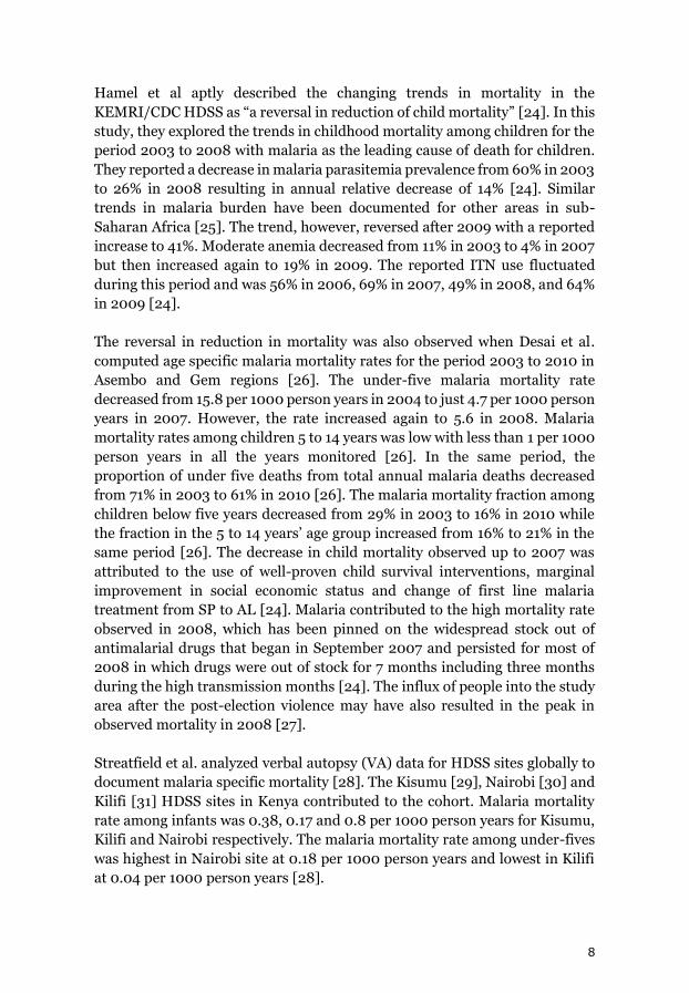
Hamel et al aptly described the changing trends in mortality in the

KEMRI/CDC HDSS as “a reversal in reduction of child mortality” [24]. In this

study, they explored the trends in childhood mortality among children for the

period 2003 to 2008 with malaria as the leading cause of death for children.

They reported a decrease in malaria parasitemia prevalence from 60% in 2003

to 26% in 2008 resulting in annual relative decrease of 14% [24]. Similar

trends in malaria burden have been documented for other areas in sub-

Saharan Africa [25]. The trend, however, reversed after 2009 with a reported

increase to 41%. Moderate anemia decreased from 11% in 2003 to 4% in 2007

but then increased again to 19% in 2009. The reported ITN use fluctuated

during this period and was 56% in 2006, 69% in 2007, 49% in 2008, and 64%

in 2009 [24].

The reversal in reduction in mortality was also observed when Desai et al.

computed age specific malaria mortality rates for the period 2003 to 2010 in

Asembo and Gem regions [26]. The under-five malaria mortality rate

decreased from 15.8 per 1000 person years in 2004 to just 4.7 per 1000 person

years in 2007. However, the rate increased again to 5.6 in 2008. Malaria

mortality rates among children 5 to 14 years was low with less than 1 per 1000

person years in all the years monitored [26]. In the same period, the

proportion of under five deaths from total annual malaria deaths decreased

from 71% in 2003 to 61% in 2010 [26]. The malaria mortality fraction among

children below five years decreased from 29% in 2003 to 16% in 2010 while

the fraction in the 5 to 14 years’ age group increased from 16% to 21% in the

same period [26]. The decrease in child mortality observed up to 2007 was

attributed to the use of well-proven child survival interventions, marginal

improvement in social economic status and change of first line malaria

treatment from SP to AL [24]. Malaria contributed to the high mortality rate

observed in 2008, which has been pinned on the widespread stock out of

antimalarial drugs that began in September 2007 and persisted for most of

2008 in which drugs were out of stock for 7 months including three months

during the high transmission months [24]. The influx of people into the study

area after the post-election violence may have also resulted in the peak in

observed mortality in 2008 [27].

Streatfield et al. analyzed verbal autopsy (VA) data for HDSS sites globally to

document malaria specific mortality [28]. The Kisumu [29], Nairobi [30] and

Kilifi [31] HDSS sites in Kenya contributed to the cohort. Malaria mortality

rate among infants was 0.38, 0.17 and 0.8 per 1000 person years for Kisumu,

Kilifi and Nairobi respectively. The malaria mortality rate among under-fives

was highest in Nairobi site at 0.18 per 1000 person years and lowest in Kilifi

at 0.04 per 1000 person years [28].

9

Risk factors for malaria transmission

Physical environment

Temperature

The development and survival of the mosquito vector that transmits malaria

depend on environmental factors such as temperature and precipitation. The

spatial limits of distribution of malaria is affected by environmental suitability

of malaria vectors where temperature plays a pivotal role [32, 33].

Temperature modulates endemicity in some areas and prevents transmission

in others [10, 32, 34]. This explains why stable malaria transmission is

restricted to the tropics [35-37]. Future climate scenarios show a warming

planet with changes in length of transmission season for malaria. The

highland regions in East Africa are projected to see an increase in the persons

at risk of malaria with increasing temperature [35, 38-40]. Temperatures

above 220C has been shown to be suitable for stable malaria transmission

while temperature above 320C result in high vector mortality [36].

Since insects are ectothermic, their development greatly depends on

temperature. They are also poikilothermic meaning their metabolic rates are

determined by temperature. Low temperature results in larger insects as they

take long to develop to adult stage. Bayoh et al. evaluated the effect of

temperature on the aquatic stages of An. gambiae from egg to larva. They

found that the optimal development temperature was between 28-320C and

for mosquito production between 22 -260C. Below 160C and above 340C no

vector could develop [41-43]. In the coastal and western regions of Kenya,

temperature was found to negatively correlate with populations of An.

gambiae and An. arabiensis [21, 44]. Kirby also showed that vector survival

decreased with increasing temperatures and larval stage duration decreased

with increasing temperature. The survival of An. arabiensis was 65%, 59% and

below 40% at 250C, 300C and 350C respectively and larval stage duration was

12.2,10.5, and 10.5 days for the same temperature ranges [45]. Higher mean

water temperature has been shown to lower larval duration by four days in

two sites in Kenya [46].

Malaria parasite sporogony cycle, the time it takes for sporozoites to appear

in salivary glands of the mosquito after an infected blood meal, is also affected

by temperature. Blanford et al used thermodynamic parasite model to assess

temperature effect on extrinsic incubation period (EIP) of malaria parasite at

four sites in Kenya with varying climatic conditions [47]. EIP is the time it

takes the parasite to develop inside the mosquito after an infected blood meal

to the time of transmission to another host. They used different time

10

resolution for temperature, monthly, daily and hourly means. In all the four

areas, the temperature parasite development relationship was non-linear with

an inverted U-shape. For Kisumu the parasite development increased linearly

from 160C peaking at 310C then steadily declining [47]. In warmer

transmission areas, EIP increased with the finer the temporal resolution of

mean temperature. For example, in Kisumu, using the monthly temperature

EIP took 12.5-16.5 days while using hourly temperature, EIP took longer (15-

18) days [47]. Diurnal temperature fluctuations can also alter incubation

period of parasites [48], mean temperature of below 210C has been shown to

speed parasite development while one above 210C slowing development [49].

Minimum and maximum temperature was shown to correlate with

entomological inoculation rates. A correlation of -0.36 and 0.24 was found for

maximum and minimum temperatures with An. gambiae human biting rate.

The effect was pronounced when lags of temperature indicators were taken

into consideration [50].

Rainfall and humidity

Rainfall provide breeding sites for mosquitoes to lay their eggs. For example,

rainfall frequency and intensity determine pond stability for vector breeding

[51]. The amount of rainfall, in combination with wind and temperature, also

determines the levels of relative humidity (RH). RH, which is the amount of

water vapor in the air, influences mosquito vector relative abundance [42, 52,

53]. RH of above 55% was shown to determine malaria survival [53], while

Bayoh et al. showed that vector survival increased with high levels of RH. The

peak vector life expectancy was determined for RH of 100%. 40% was the

minimum RH necessary for vector survival [42].

An. gambiae vectors breed in temporary and turbid water provided by rain

[36]. Mosquito densities have been show to increase during the rainy season

[54], followed by more malaria associated febrile illnesses [55]. Malaria

incidence was shown to be higher in areas with high water accumulation [56]

High water accumulation has been depicted as having strong linear

relationship with malaria presentation [57], and to be significantly associated

with occurrence of malaria parasites [58]. However, excessive rainfall can

flush existing mosquito larvae temporally resulting in reduced vector

population and, thus, malaria incidence. This results in a non–linear

relationship between rainfall and malaria health indicators as shown in [59-

61] where malaria increases with increasing rainfall, peaks then falls at the

extremes

In permanent water environments, predation determines water malaria

vector populations. The larvae of mosquitos stay at the surface of water where

11

they are adapted to feed and obtain atmospheric oxygen [42]. Craig et al.

determined that five months of rainfall above 80 mm in a year was sufficient

for malaria to occur if all the other requirements are met, and when

temperatures are high, only three months of rainfall above 80 mm was

sufficient for stable malaria transmission [36]. Vector biting rates have also

been found to correlate with the amount of precipitation [50, 62]. Patz et al.

found a correlation between the amount precipitation and An. gambiae

human biting rate with a lag of up to four weeks [50]. Amek et al found no

significant relationship between precipitation and mosquito density; however,

mosquito density peaked in the month of May during the rainy season [21]. In

drier savannah region where annual rainfall amounts fall below 1000 mm, An.

arabiensis species of mosquitoes proliferate [63]. In these regions, the peak

of mosquito density has been determined to correlate with rainfall seasons

with significant correlations observed with a six week lag [64]. Further, a

correlation of 0.87 has been found with five months of rainfall in a year [65],

and two months lag of rainfall in east African highlands [66]. Moisture index

also determines mosquito species composition with an index above 0.7 found

suitable for An. gambiae while index below 0.7 are suitable for An. arabiensis

[67].

Land cover

Satellite derived data has been used widely in malaria epidemiology. The most

commonly used remote sensed land cover proxy is normalized difference

vegetation index (NDVI) [68, 69]. Vegetation is very reflective in the near

infrared and absorptive in the visible red. The ratio of these can be used as an

indication of the status of vegetation [70]. This ratio ranges between -1 and 1,

with higher values showing denser vegetation, 0 signifies lack of vegetation

and -1 representing water bodies. A decrease in vegetation index may mean a

decrease in vegetation density thus water availability. It could also mean

suppression of vegetation due to flooding [71].

Land cover especially vegetation, provide suitable resting and sugar feeding

places for adult mosquitoes and creates the right microclimatic conditions for

mosquito proliferation. Vegetation state monitoring and mapping of water

bodies is crucial in identifying sources of malaria vectors [72]. Many studies

have explored the correlation between NDVI and malaria transmission

factors. For example, in Nigeria NDVI was singled as an important variable

for malaria risk assessment [73], shown to positively correlate with mosquito

density [21, 74-76]. NDVI is also correlated with mosquito biting rates, with

biting rate transient in high NDVI areas [62] and negatively associated with

mosquito larval densities in and around ponds [77].

12

NDVI has been used to develop malaria predictive models showing different

lag patterns [78] between NDVI levels and malaria incidence. In Kenya,

Burundi and Ethiopia, malaria in a given month was best predicted by average

NDVI of the previous month [57, 79-81]. Malaria has been shown to correlate

highly with low levels of NDVI; low NDVI was associated with abundance of

mosquito vectors along the coast of Kenya [44], a threshold of 0.3-o.4 resulted

in 5% increase in malaria presentation in Kenya [57], and low NDVI was

associated with increased number of malaria cases in Bangladesh [82].

However, in West Africa higher NDVI were associated with malaria infections

in children [83]. Distance to vegetation has also been associated with

Anopheline aggressiveness [84]. Exposure to forest areas has also been linked

with upsurge of malaria infections [85], and high risk has been reported for

houses surrounded by green vegetation [86].

Socio-economic factors

Education and economic status

Education, economic status and outdoor activities in endemic areas [87] also

affects the odds of one being at risk of malaria. It has been proven that low

education and economic means increases the risk of malaria infection [88]

and working outdoors [89], having high household wealth [90-92], and high

education level for the caregiver [93, 94], provide protective effects. High

social economic ability is associated with high mosquito control [95] and,

thus, the low risk observed.

Human practices

Human activities that alter land cover affect the mosquito population levels.

In highlands and lowlands of Western Kenya, an increase in farmland use

provided suitable environment for An. gambiae larva development [96, 97].

Mature maize fields, newly cultivated fields, grassland [97] and agro-

ecological zones [76] were correlated with presence of mosquito larval

habitats and irrigated fields associated with malaria parasitemia [98]. It has

been shown that areas where land cover has changed due to deforestation

experience high rates of malaria [99, 100] as new breeding sites are created .

Malaria transmission risk increases among those living in proximity to

stagnant water (OR=2.1) [101], permanent ponds [102] or near breeding sites

[100, 103, 104] and in areas with irrigated land (RR=2.68) [105] and wet

lowland (OR=4.45) [106].

13

Housing conditions

Housing characteristics also affect malaria risk. Living in houses with

thatch/mud roof and mud floors increased the odds of malaria risk [107]. In

Uganda, it was shown that houses with earth/sand floors increases odds of

malaria (OR=2.65) and sand/dung floor having odds of (OR=1.8) [93] as

compared to finished surfaces. In Burkina Faso, having earth brick floor

protected (OR=0.2) households against malaria infection while stone floor

increased risk [108]. It has been shown that living in earthed roofed houses

and sleeping in same room with animals increased risk of malaria infection by

a magnitude of 2.5 and 1.8 respectively [105]. The type of house wall material

and living in areas with high housing density has also been shown to amplify

risk to malaria [89, 109]. Having a wooden or mud house has been associated

with increased risk (OR=1.32) in Rwanda [86] and OR=1.63 in Eritrea [106].

Houses with holes also increase odds of malaria (OR=1.59) as shown by

Woyessa et al [110]. Household size has been shown to negatively correlate

with malaria [111].

Prevention measures

The huge gains in the global malaria burden reduction can be attributed to

significant increase in access and utilization of malaria prevention strategies.

For example, in 2015, 67% of households in sub-Saharan African had access

to ITN compared to 56% in 2014 with 82% of the households with access

actually using them. The proportion of the population sleeping under ITNs

increased from 46% in 2014 to 55% in 2016 with the proportion of under-fives

sleeping under ITN seeing a major leap from <2 % in 2000 to 68% in 2015 [9].

In Kenya, through the KIMS, it was reported that 63% of the households had

at least one long lasting insecticidal nets (LLINs) in 2015 compared to 44% in

2010. 40% of the households had 1 net for two people. 48% of the people in

the households slept under a LLIN the previous night prior to interview. LLIN

usage depended greatly on ownership with 71% of the households with at least

one LLIN sleeping under LLIN. There was an increase in the proportion of

children sleeping under LLINs from 39% in 2010 to 56% in 2015. The

percentage of pregnant women sleeping under LLINs also saw an upward

trajectory with an increase of 22% from 36% in 2010 to 58% in 2015. The

increase in net coverage was observed in high risk areas including the lake,

coastal and epidemic highland regions [11].

The Kenya malaria control strategy recommends pregnant women to receive

intermittent preventive treatment (IPTp) as prophylaxis against malaria

during antenatal care. From KIMS 2015, 75% of the pregnant women who

14

delivered two years preceding the survey received at least 1 dose of

Sulfadoxine/Pyrimethamine (SP)/FANSIDAR, 56% received at least 2 doses,

while 37% received the three recommended doses [11].

One of the pillars of the Kenya malaria control strategy includes prompt

parasitological diagnosis and treatment within 24 hours of onset of symptoms.

In the 2015 survey, 7 out of 10 children presenting with fever were taken to

health facilities for medical advice with 72% receiving treatment. 39% of the

children had their blood taken for testing while 25% got the recommended

Artemisinin combination based therapy (ACT) [11].

Prevention in epidemic situations

The control measure to be used when in epidemic malaria situation depend

on the time window to act. Early detection of epidemics provide shorter lead-

times, and consequently individual case management is preferred to reduce

mortality and morbidity. The drugs used in individual case management

should have at least 95% efficacy. Currently ACT has been widely used in

treating uncomplicated P. falciparum malaria [112] and intramuscular

injectable Artemether for severe presentation of malaria. ACT can also be used

for mass fever treatment [113]. The huge reduction in malaria burden in sub-

Saharan African has been attributed to ACT [114]. In Kwazulu Natal in south

Africa Artemether/Lumefantrine (AL) was used to control epidemic malaria

with significant reduction in both outpatient and inpatient admission due to

Malaria [114]. AL was also instrumental in reducing mortality due to malaria

in Tigray region of Ethiopia during the May–October malaria epidemic [114].

In regions with medium to high levels of transmission, mass screening and

treatment (MSAT) can result in lower malaria burden as shown by Crowell et

al in Sub–Saharan countries [115]. Mass screening of the community and

treatment with AL can reduce transmission in high malaria endemic regions

[116].

If an epidemic has been predicted and there is sufficient time to act, vector

control measures provide better option to curb the high risks of mortality and

transmission associated with epidemics [113]. The vector control activity

should be well planned, targeted and timely. Vector control as an intervention

is most effective when used at beginning of an epidemic and with high

coverage >85% of the epidemic risk region.

Vector control works to curtail the reappearance of malaria in a previously

controlled area and to prevent gradual transmission increase over the years or

increase in annual seasonal transmission. The most widely used vector control

strategy is Indoor Residual Spraying (IRS). It is recommended that the spray

15

chemical used in IRS campaigns should have a residual action beyond 6

months. Synthetic pyrethroids have been shown to be effective and provide

residual action of between 2-6 months. The spraying of houses to get rid of

mosquitoes has been shown to lower risk of malaria infection [93]. Spraying a

household in the last six months reduced the odds of malaria infection

(OR=0.26) in Eritrea [106].

The use of ITNS may not be very effective in epidemic situations but could be

useful to reduce morbidity in endemic regions where coverage is high. In

Ethiopia Alemu et al showed that the odds of malaria infection increased for

those not using ITN [88, 101, 109, 117, 118] with an odds ratio of 13.6 [101].

Larval control is another intervention that may be less useful in epidemics but

may prove effective when breeding sites are fewer, known, permanent and

accessible [113]. Several studies have shown the efficacy of using both IRS and

ITN in malaria control. In Western Kenya highlands characterized by malaria

epidemics, IRS was shown to reduce parasitemia by up to 64% in intervention

areas with effect persisting for six months [119].

In the countries with high malaria transmission burden, a combination of

both IRS and ITN significantly reduced malaria parasitemia prevalence [120-

126]. It has also been shown that using a combination of IRS with rounds of

Dichlorodiphenyltrichloroethane(DDT) and MSAT, it is feasible to lower

parasitemia prevalence in moderate transmission settings in Africa, however

higher coverage levels of over 90% is necessary to achieve similar reductions

in high transmission environments [127].

Malaria surveillance

Public health malaria surveillance systems comprise detection, registration,

confirmation, reporting, analysis and feedback [128]. The main purpose of the

surveillance is to inform policy and improve timely response [129].

The action included in surveillance system includes acute response and

planned responses, which are supported by communication, training,

supervision and resource provision [128]. Activities included in the response

system include confirming diagnosis through laboratory testing, active case

finding, collection of clinical and environmental data, synthesis and

interpretation of data [129].

16

Malaria early warning and detection

Malaria epidemics affect populations with less immunity in highlands and

semi-arid areas of Africa and occur due to increase in temperature which is

normally low [130]. One of the targets of the Roll Back Malaria initiative is to

detect malaria epidemics within two weeks of onset. Early detection and

prevention of malaria outbreaks is a key pillar in malaria control strategy. An

early warning system has been aptly defined as “The provision of timely and

effective information, through identified institutions, that allow individuals

exposed to hazard to avoid or reduce the risk and prepare for effective

response” [131].

An early warning system for malaria control in Africa has been formulated by

WHO through a framework [132]. The malaria early warning (MEW)

framework involves the use of vulnerability, transmission risk, and early

detection indicators. Vulnerability factors include immunity levels, migration,

malnutrition and HIV while transmission risk may include factors such as

rainfall and temperature. Early warning indicators can be obtained through

routine case reporting and using set thresholds to issue alerts [132]. The use

of malaria early warning system in epidemic prone regions has been

recommended in order to optimize lead times for control managers to act

[133-135]. Abeku et al have advocated for improved malaria surveillance to

beef up early detection capacity in malaria epidemic prone regions in Africa

[130] in current focus to achieve targets set for malaria in the Sustainable

Development goals [9]. Lindblade showed that monitoring mosquito density

can also be used for early warning [136]. With improvement in surveillance, it

would be possible to precisely determine when an epidemic begins.

Combining surveillance data and malaria risk factors, predictive models can

be developed to provide early warnings for effective responses.

Early detection

Early detection techniques with thresholds computed from baseline data have

been used in malaria control in different epidemiological settings. Cullen

showed that using historical malaria patterns, it was possible to detect

departures from normal transmissions in Thailand. Any incidence greater

than two standard deviations from normal mean were flagged as anomalous

[137]. The Cullen method above for early detection was used also in endemic

areas in Zambia where upper confidence limit was used as threshold for

detection [138].

The highland malaria project set up surveillance in 20 sites in Kenya and

Uganda to detect abnormal malaria incidence in these sites [139]. Utilizing an

17

automated system, aberrations were detected based on weekly and region

specific levels of malaria incidences compared to baseline values from the

previous seven years of data. The anomalous weekly incidences were

computed by taking a difference of particular week from the de-trended mean

and dividing by the baseline standard deviations [139].

Malaria forecasts

Historical malaria case surveillance data can be modelled to make short-term

predictions. In Ethiopia, a seasonal adjustment method was used to make

forecast with one-month lead using historical data [140]. The relationship

between malaria incidence and climatic factors [78, 141, 142] has also been

exploited to develop prediction models that could act as early warning systems

with varied lead times. For example, remote sensing derived precipitation was

shown to correlate with malaria incidence anomalies in Eretria with a lead-

time of two to three months [143], real time rainfall monitoring has been used

as an operational epidemic warning system [144], remote sensing data used

to predict malaria incidence in epidemic prone areas in Kenya [145]. Hay

showed that rainfall data gave timely and reliable early warning for the 2002

malaria epidemic in Kericho, Kenya [146]. In Ethiopia, rainfall, vegetation

index (VI) and evapotranspiration (ETA) provided prediction lead times of

one to three months [81], and use of weather factors and including previous

malaria cases provided a lead time of one month [147]. Thomson et al

parameterized a non-linear quadratic relationship between rainfall and

malaria to predict anomalous malaria months. The rainfall data provided

warning on high transmission years before the peak seasons [61].

Longer lead times for predictions can be achieved using seasonal climate

forecasts [148-151]. Using seasonal climate forecasts in India, the model was

able to identify high and low malaria years with high skill with three month

forecast lead time [149]. In Botswana, a four-month lead time was achieved

using seasonal climate forecasts data to forecast probabilities of high and low

malaria incidences with high precision [151].

Evaluating economic benefit of early warning systems

In most areas that experiences malaria epidemics, MEWS are not yet fully

functional. Because of this, it is possible to evaluate only certain components

of their roles such in reduction of number of cases by use of interventions such

as vector control strategies. The type of information used in providing forecast

determine the timing of interventions that is crucial in assessing economic

benefit of MEWS. Making comparisons between different intervention

18

strategies with and without MEWS, offer means to measure the economic

benefit of having a MEW in place.

Drummond defines economic evaluation as “the comparative analysis of

alternative courses of actions in terms of their costs and consequences”. Some

of the methods used in economic evaluation includes, cost minimization

analysis, cost effectiveness analysis, cost utility analysis and cost benefit

analysis. In the assessment of economic value of early warning systems, either

of the following two approaches can suffice. One is analyzing users of the

systems willingness to pay referred to as contingent valuation. The other is

cost avoidance calculations which utilizes statistical procedures to perform

cost estimations to evaluate damage prevented if warning is in place and

compares with resources needed set in place and operationalize the system

[152]. To perform an economic evaluation of an early warning system we

would need to know the investment costs, maintenance and repair costs and

operating costs [153].

Some of the factors that affect effectiveness of MEWS include personal and

cultural factors, prediction related factors and dissemination related factors.

The prediction related factors include type I errors which are missing alerts,

type II errors which are false alerts [152]. The overall operational cost of the

system, societal economic losses arising from false alerts an societal savings

should be computed to appreciate the cost benefit of the early warning system

[154].Worrall et al. performed a cost effectiveness analysis to determine the

effectiveness of using A MEW with insecticidal residual spraying program for

Zimbabwe [155, 156]. They compared different levels of coverage of IRS with

varied timing to the do nothing strategy which was taken as having no MEW

in place. The do nothing assumed a coverage of 0% thus representing situation

with warning [156]. The indicators used for economic evaluation were, the e

total number of cases each year per intervention scenario, the incremental

cost of spraying compared to do nothing, the incremental cost per case

prevented compared to do nothing, the total cost of malaria control and the

net incremental cost per case prevented compared to do nothing [156].

Economic evaluation of early warning with uncertainties in

prediction

Predictive information emanating from early warnings are seldom used by

disease control managers due to the level of uncertainty associated with the

forecasts. With low prediction accuracies, the benefits of interventions could

be hard to tease out and thus public health officials not use the information to

take preventive measures [157]. Decision makers that act based on predicted

19

events may suffer if the alarm is false. It has been shown that this information,

however uncertain could still be very useful to decision makers [157].

Early warnings should be provided well in advance to allow sufficient lead

time to take action. However, as the lead time increases, the uncertainty

associated with the predictions increases [131] such as the uncertainties

inherent in seasonal weather forecast that provide longer lead times. Schröter

et al illustrate the interplay between lead time and warning reliability in Figure

5. in its application to early warning for flash floods [153].

Figure 5. Warning reliability as a function of lead time (source: [158])

Every prediction given has some error attached to it that would either result

in a false negative, a false positive or difference in predicted and observed

cases. Every warning message should include the level of uncertainty and the

expected cost of taking action [131]. To improve the performance of EWS,

decision-making should include the expected consequences of taking action

in terms of probability of a false and a missed alarm. An acceptable level of

probability of false alarm should be set using a threshold and included in the

economic evaluation. The incidence of false and missed alarms can be greatly

reduced by factoring in uncertainty and the corresponding action taken [131].

20

Summary

We have seen that several factors act together to modify populations risks to

malaria infections. Environmental risk factors; including rainfall,

temperature and land cover characteristics; vector control methods such as

IRS and use of LLINs affect vector abundance and competency to transmit

malaria. Human behavior such agricultural practices, health seeking patterns

and economic means determine the malaria burdens experienced by

households. Monitoring these indicators through robust surveillance system

provide mechanism to quantify the relationships and improve management of

risks. In order to have better control and effective use of available

interventions, understanding these dynamics and using the information in

developing systems that help predict levels of expected future caseloads can

result in progress towards achieving malaria elimination especially in areas

burdened by malaria. To increase the sustained utilization of predictive

systems among public health officials, uncertainties in predictions and

intervention effectiveness should be considered jointly and strategically.

21

Objectives

The main aim of this study was to assess the prospects and feasibility of using

climate and environmental information to forecast malaria incidence in

Western Kenya, and to develop a methodological economic framework

assisting decision making of time sensitive counter measures responding to

forecasts. Our contribution to an early warning system is illustrated in Figure

6. The specific objectives were to:

I. Determine the association of weather variability and under five

malaria mortality using data from KEMRI/CDC HDSS

II. Evaluate the association of remotely sensed environmental conditions

and malaria mortality in three malaria endemic regions in Western

Kenya

III. Use remote sensing environmental data to forecast malaria incidence

at a rural district hospital in Western Kenya and evaluate forecast

accuracy

IV. Develop a methodological framework to integrate economic impact

models of operational response to forecasts and their uncertainty

Figure 6. How the thesis papers contribute to core components of early warning systems.

22

Materials and methods

Study setting

We extracted the health outcome data was from the KEMRI/CDC Health and

Demographic surveillance system (HDSS). In most poor countries, vital

registration data such as births and deaths are often incomplete, thus the

HDSS framework provides complete data by collecting demographic

information from all residents in geographically defined regions in a country

[159-161]. There are several HDSS sites in Africa and Asia under the umbrella

body INDEPTH network [160] with a systematic collection of health and

demographic data. The database is available online for researchers [162].

The KEMRI/CDC HDSS [20, 29] is conducted at three contiguous sites in

Western Kenya about 60km away from KISUMU County. Today, the

KEMRI/CDC HDSS follows a population in three geographically defined

areas. The first site to be enumerated was Asembo in 2001, followed by Gem

in 2002 and Karemo in 2007. The HDSS covers an area of about 700 km2

located at latitudes ranging from -0.210 to 0.130 and longitudes ranging from

34.16o to 34.520. The topography of the HDSS area comprises gentle hills and

valleys with a number of streams and rivers. The map of the HDSS area is

shown in Figure 7. The surveillance commences with a baseline census, after

which regular census are conducted to update the population. Residency

status in the surveillance is gained by staying in the study area for four

calendar months or being born to a resident [20, 29].

Figure 7. Maps of Africa, Kenya, Western Kenya and the KEMRI/CDC HDSS Study sites Karemo,

Gem and Asembo (source: [29]).

23

The population changes through demographic processes such as births,

deaths and migrations. In the KEMRI/CDC HDSS, three censuses are

conducted in a year. Besides births, deaths and migrations, a myriad of other

information is collected from the residents. These include education levels,

ownership of household assets used to construct wealth quintiles [163], house

structures, marital status, immunization status for children and cause of death

data derived using verbal autopsy [20, 29]. The HDSS has provided a

sampling frame for conducting several surveys for other research projects

using the population data. The KEMRI/CDC HDSS supports TB, Malaria, and

HIV projects within the KEMRI/CDC public health collaboration. The health

component of the HDSS also involves collecting data on morbidity at health

facilities in the HDSS areas. Inpatient information is collected at Siaya district

hospital located in Karemo area while outpatient data are collected at Ting’

Wangi and Njenjra Health facilities located in Karemo and Gem respectively

[20, 29].

From the 2012 annual report, there were 42,569 compounds with 58,720

households in the study area. The median number of individuals in a

household was four. Each compound has at least one house separated by

agricultural field. The total population under surveillance was 240,633

residents. The residents by area were 69,472, 86,279 and 84,882 in Asembo,

Gem and Karemo respectively. 53% of the population were females while

children below 15 comprise 45% of the population. Children below 5 years

comprise 15% of the population while the elderly, those 65 years or above,

formed only 5% of the population. There were 7,205 births in 2012. The

population structure is typical for a developing country (Figure 8).

The crude death rate, under five mortality rate and infant mortality rate were

10, 18 and 50 per 100o person years respectively with a life expectancy of 59

years at birth. The general fertility rate was 132 per 1000 women in

reproductive age group with a total fertility rate of 4 children per woman. 87%

of children 6-10 years are enrolled in school in the study area. The houses in

the study area are made of mud, brick or cement with thatched or iron sheet

roofs [20]. Subsistence farming is the main economic activity. During normal

years, the normal annum is characterized by two rainy seasons stretching from

March to May and November to December.

24

Figure 8. Population pyramid for the KEMRI/CDC HDSS Study sites (Asembo, Gem and Karemo

2012)

Verbal autopsy

Poor countries often lack complete reporting of vital statistics such as deaths

and births. Autopsies are often not conducted on all deaths, thus getting

reliable estimates on causes of death at population levels is impeded. To

circumvent this shortfall, verbal autopsy (VA) has been recommended for use

in poor resource setting [164-167]. Verbal autopsy involves the collection of

signs and symptoms the diseased suffered prior to death. This information is

then used to prescribe a probable cause of death. Deaths in the KEMRI/CDC

HDSS are collected using a dual system. One involves the use of village

reporters who report all deaths that happen even for non-resident members

as soon as they occur. The other is the usual surveillance conducted by

community interviewers who visit the households every four months. The

prior was included to provide timely reporting of both deaths, births and

currently pregnancies to capture neonatal deaths. When a death occurs, one-

month mourning period is allowed and then VA interviewers are sent to

conduct interview with the caregiver of the diseased prior to death. The VA

questionnaire is a standardized questionnaire such as [168, 169] collecting

symptoms for different demographic categories such as age and gender. The

VA process in the HDSS has been described in previous studies [20, 23].

25

Assigning cause of death

There are two main ways of assigning probable cause of death to signs and

symptoms collected using VA. The first one is physician coding where the VA

questionnaire is given to two or more physicians to review and come up with

a probable cause. The second system, which has increased in popularity in the

recent years, is the use of computer based statistical methods to proffer

probable causes of death from VA. The most used is the INTERVA method

[170-172]. In the KEMRI/CDC HDSS physician coding was used up to 2008

after which INTERVA method was adopted. The physician coding involved

giving two clinicians the VA questionnaires to review. They would come up

with three probable causes of death, which would be compared using a

computer algorithm. The cause that matched from the two clinicians would

be assigned as the probable cause of death. If no match was found, a third

clinician would be asked to also review the VA questionnaire and come up with

a cause of death, which would again be compared. If still no match, an expert

panel would be setup to come to an agreement. From, 2009, all the data from

the VA questionnaires were converted to INTERVA format, which is a series

of variables in binary format detailing presence or absence of symptoms. The

INTERVA methods is more systematic [170] and not prone to biases

encountered with the physician coding which would depend on experiences

and qualifications of the people reviewing the VA questionnaires. The

INTERVA methods uses the Bayesian framework that incorporates expert

opinion to give prior probabilities of certain diseases given presence of a set of

symptoms [170, 171]. The INTERVA methods includes toggle buttons to cater

for areas with high prevalence of HIV and Malaria such as the KEMRI/CDC

HDSS.

Hospital surveillance

The KEMRI/CDC collects information on morbidity at different health

facilities in the study area. The inpatient data is currently collected at Siaya

district hospital while outpatient data is collected at two health facilities,

Njenjra and Ting’ Wangi. All children admitted at Siaya district hospital have

their blood samples taken and tested for malaria parasites.

26

Environmental data

MODIS Remote sensing data

Two Moderate resolution imaging spectro-radiometer (MODIS) satellite

sensors were deployed by international earth observing system run at NASA

to aid in the global studies of the atmosphere, land and ocean processes. The

morning platform with overpass times of 10.30 am and 10.30 pm in

descending and ascending modes respectively called terra was the first to be

launched in December 1999. The second afternoon platform called aqua was

launched in May 2002 with overpass times of 1.30 pm and 1.30 am in

ascending and descending modes respectively [173]. The MODIS instruments

sweep the earth at ±55 nadir in 36 bands. Bands 1-19 and 26 are in visible and

near infrared ranges while the rest of the bands are in thermal infrared from

3-15µm [174]. The sensors take images of reflections during the day and

emissions at night or day every one to two days. Due to global coverage and

great radiometric resolution, the MODIS satellites are very useful in the study

of earth processes.

MODIS Land surface temperature

Land surface temperature (LST) is a crucial indicator of physical processes in

surface energy and water’s spatio-temporal equilibrium. LST has been used in

the study of evapotranspiration, climate change, hydrology and vegetation

monitoring[175]. LST is computed from the radiations emitted from the land

surface such as vegetation or soil surfaces at instant viewing angles [173]. The

single infrared channel and split window [174, 176] methods are used to

estimate LST from satellites. The split window method corrects for the effect

of atmosphere and been used to compute MODIS LST products [177]. The

MODIS LST products are created through spatial and temporal

transformations to daily and 8-day gridded product.

The datasets are archived in hierarchical data format- earth observing system

(HDF-EOS) [177]. The MOD11A1 daily LST product at 1km resolution is

generated from the MOD11_l2 product by mapping the pixels to a day in a

earth location on sinusoidal projection [177]. The datasets are generated at tile

level, which is 1113 km by 1113 km with 1200 rows, by 1200 columns. The

MODIS tiles downloaded for this study are h21v08 and h21v09 that covered

the KEMRI/CDC HDSS area. The MODIS MOD11A1 LST product scientific

datasets extracted for this study were lss_day_1km, qc_day, lst_night_1km

and qc_night. The variables with qc prefix are for quality assurance [177].

27

MODIS Vegetation Index

Vegetation indices (VI) are transformations of two or more spectral bands that

can aid in the robust spatial and temporal comparisons of photosynthetic

activity and canopy variation[178]. They are indicators of vegetation growth

and vigor [179]. The MODIS VI are designed to provide consistent spatial and

temporal comparison of global vegetation conditions. The two VIs are NDVI

and Enhanced vegetation index (EVI). While NDVI is sensitive to chlorophyll

characteristics, EVI is more correlated to canopy variations. The MODIS

NDVI has been described as the ‘continuity index’ [180], it increases the

temporal extent of the NOAA-AVHRR derived NDVI time series. NDVI is the

normalized ratio of the near infrared (NIR) and the red bands.

𝑁𝐷𝑉𝐼 =𝜌𝑁𝐼𝑅 − 𝜌𝑟𝑒𝑑

𝜌𝑁𝐼𝑅 + 𝜌𝑟𝑒𝑑

Where 𝜌𝑁𝐼𝑅 and 𝜌𝑟𝑒𝑑 are the surface bidirectional reflectance factor in their

respective MODIS bands. NDVI has been used widely because of its stability

in the identification of seasonal and inter-annual changes in vegetation

growth and activity. However, the NDVI ratio is non-linear and prone to

additive noise effects like cloud cover [178]. Gridded VI maps are generated

using surface reflectance corrected for molecular scattering, ozone absorption

and effects of aerosols [180]. The VI algorithms use the upstream surface

reflectance (MOD09) product to temporally composite the images to create

the VI products [181]. Maximum value compositing (MVC) method is used to

create the composite VI products. In the MVC algorithm, several images over

a given time interval are merged by taking the input pixel with the highest

NDVI value to create a single cloud free image [180-182]. Some of the

objectives of compositing include; depiction and reconstruction of

phenological variations and to maximize global and temporal coverage [182].

The MODIS VI are produced at 250 m, 500 m, 1 km and 0.05 degrees spatial

resolution. The MODIS VI are also produced in tiles which measure about

1200 km by 1200 km and mapped in the sinusoidal grid projection [181].

There are six MODIS VI products but for our purposes, we used the MOD13Q1

16 day 250 m VI product. The MOD13Q1 is generated using the daily MODIS

level 2G surface reflectance product. The MODIS VI data products are stored

in HDF-EOS format [181].

28

MODIS data for the study area

Both of the MODIS products MOD11A1 for LST and MOD13Q1 for NDVI used

in this thesis are stored in the HDF-EOS format. The data is available for

download at different tiles covering different geographical regions. We

downloaded two tiles, h21v08 and h21v09 that spanned the KEMRI/CDC

HDSS study areas. We downloaded data for the period 2002 to 2013. The

downloaded HDF files were mosaicked together, and re-sampled using the

Nearest neighbor (NN) method and re-projected to a geographic map creating

TIFF images using the MODIS projection tool [183]. Data from the TIFF

images were extracted using RGDAL [184] package in R environment. The 16

day MODIS NDVI data was interpolated using natural cubic spline to get daily

estimates while the missing daily values for LST were linearly interpolated

using the TIS [185] package in R.

Tropical rainfall measuring mission (TRMM)

Rainfall data used in this study were extracted from the TRMM satellite data

available online. TRMM is a joint project between Japan and USA. TRMM was

launched by H-II rocket from National space development space agency of

japan (NASDA)/TANAGASHIMA space centre in November 1997 with a

circular orbit of 350 km off the earth’s surface [186]. TRMM was launched to

observe the rate, structure and spatial distribution of rainfall in tropical and

subtropical regions and it is the first space mission dedicated to measuring

tropical and subtropical rainfall. Tropical rainfall contributes over two thirds

of the global rainfall amounts and, thus, its knowledge is crucial in

understanding and predicting global climate system. TRMM satellites use

microwave and infrared sensors. The data from TRMM satellites are received

at NASA ground station via tracking and data relay satellite [186]. We

downloaded data for the years 2002 to 2013 from NASA’s Tropical Rainfall

Measuring Mission (TRMM) as binary files at 0.250 x 0.250 spatial resolution

and daily at three-hour intervals temporal resolution. To get total daily

precipitation estimates, we multiplied the hourly rates by 3 and summed.

Ground weather data

The ground weather data used in this study was retrieved from the Kisumu

weather station located at Kisumu airport. The data used were daily rainfall,

minimum and maximum temperature. Kisumu airport is about 60 km away

from the KEMRI/CDC HDSS area.

29

Statistical analysis

Distributed lag nonlinear models

When assessing the effect of environmental factors on health outcomes, there

is usually, a period preceding observed health effects after the occurrence of

the exposure. This elapsed time between exposure and outcome is called lag

time and can be interpreted as latencies in the ecological & biological systems

of exposure and effect. The lag association will adjust for the timing and

intensity of previous (and other) exposures while estimating the exposure-

response relationship [187].

Distributed lag models (DLM) have been developed to factor in the lag

component in statistical regression modelling handling the fact that lag

variables if included directly in regression models could yield instability in the

statistical estimates due to the high temporal correlation, so called

collinearity. In the DLM framework, the latency processes of exposures on the

response is assumed to be distributed over a period of time [188]. To capture

lag and nonlinear effects, a family of models called distributed lag nonlinear

models (DLNM) have been developed [188]. The DLNM models

simultaneously describes associations along the space of the predictor and in

its lag dimension [188]. DLNMs have been shown to provide robust estimates

of effects compared to DLMs [189]. Time series of ouctome 𝑌𝑡 (𝑡 = 1, … … , 𝑛 ) is often represented by the equation below adapted from [188].

𝑔(𝜇𝑡) = 𝛼 + ∑ 𝑠𝑗

𝐽

𝑗=1

(𝑥𝑡𝑗; 𝛽𝑗 ) + ∑ 𝛾𝑘𝜇𝑡𝑘

𝐾

𝑘=1

Where μt = E(Y) and are Y assumed to arise from exponential family distribution. sj denotes smooth function of xj with parameter βj while μk

represents additional variables included in the model with coefficients γk. In

time series analysis of environmental factors to disease registries, Yt are often

counts assumed to originate from over-dispersed Poisson distribution. In

these models, smooth function of time is often included to capture effects of

confounders [188], and an offset of population at risk can sometimes be

combined with the time trends yielding and incidence model. In models

without an explicit offset the time trends will adjust for population size

changes at the time scale of the time function making parameters

approximating incidence estimates assuming population fluctuations is not

faster than the time trend adjustments.

30

Basis

The relationship between g(μ) and x can be defined by a smooth function s(x)

and included in the model as a sum of linear terms. This is done by choosing

a space of functions called basis containing s [188]. The basis functions

transform x to form basis variables. The assumption on the shape of

relationship between exposure and outcome determines the basis function to

use. Some of the basis functions used include polynomials or spline functions.

DLNM extends the basis definition by introducing a crossbasis function,

which is a bi-dimensional space of functions describing the shape along x and

its distributed lag association [188]. This involves choosing two sets of

functions, which are then combined to form the cross-basis functions [188].

The DLNM models have been implemented in the R environment and its

application is described in detail in Gasparrini et al. [190].

Interpretation of risk

The estimated relative risk contributions in the lag-response curve can be

interpreted using a forward or backward approach [187]. β̂ℓp can be the

relative risk contribution at time 𝑡 + ℓ𝑝 in the future from a unit increase in

exposure x at time t, or the contribution of a unit increase in exposure x occurring at time 𝑡 − ℓ𝑝 in the past to a given risk measured at time t [187].

Attributable Risks can be derived from DLNMs as described by Gasparrini et

al. [191].

General additive models

A generalized additive model replaces the linear part of generalized linear model with smooth functions [192]. The linear part ∑ 𝛽𝑗𝑋𝑗 in the GLM is

replaced by a sum of smooth functions ∑ 𝑠𝑗(𝑋𝑗) called the additive predictor

and thus the name. GAMs are useful in teasing out non-linear covariate

effects. The models allow flexibility on structure of response and covariates by

allowing specification of smooth functions[193]. An example of a univariate

smooth is described in the book by Wood, 𝑦𝑖 = 𝑓(𝑥𝑖) + 𝜖𝑖 adapted from[193].

In this simple model, yi is a response variable, xi is a covariate, f is a smooth

function and 𝜖𝑖 are random variables. The function f can be defined by

choosing a basis assumed to take the form:

𝑓(𝑥) = ∑ 𝑏𝑖𝑞𝑖=1 (𝑥)𝛽𝑖 from [193].

For example, for a 4th order polynomial, the space of polynomials of order 4

contains f. Expanding the 4th order polynomial results into a model of the

structure as evaluated in[193] : 𝑦𝑖 = 𝛽1 + 𝑥𝑖𝛽2 + 𝑥𝑖2𝛽3 + 𝑥𝑖

3𝛽4 + 𝑥𝑖4𝛽5 + 𝜖𝑖 . The

31

basis function can also be represented using cubic spline. Wood in the

book[193] describes cubic splines as a combination of cubic polynomials

joined forming a continuous a curve. The points where the polynomials join

are called knots, which are spaced equally in the range of x and form the basis

dimension. The number of knots determine the degree of smoothing [193].

The value of the smoothing parameter 𝜆 should be chosen to approach the true

function f. There is over smoothing when the value of 𝜆 is too high and under

smoothing when it is too low. One of the methods used is penalized regression

splines to choose 𝜆. In this method , the smoothness is controlled by fixing the

basis dimension at large size and imposing a ‘wiggliness’ penalty [193].

Generalized cross validation is one method used to choose the smoothing

parameter. This is done by leaving each data point successively and fitting

model to remaining data and calculating squared differences between left out

data and their predicted values which are then averaged across all data [193].

A very detailed introduction to GAMs and its implementation in R using the

mgcv package[194] are illustrated in the book by Wood [193].

General additive models for location, scale and shape (GAMLSS)

GAMLSS models provides a flexible framework to model the outcome

distribution called location and its distribution functions such as mean and

standard deviation together [195]. GAMBOOSTLSS [195] provides boosting

algorithm to fit GAMLSS models which are an extension of the GAM [192]

models.

Boosting

GAMBOOSTLSS fits a GAMLSS model by adopting the component wise

gradient boosting. Regression boosting methods emanated from supervised

machine learning discipline and involves iteratively fitting various predictors

using simple regression functions called base learners and then combining the

estimates at each iteration to the additive predictors. In gradient boosting,

base learners are fitted to the negative gradient of the loss function. The

algorithm sweeps through a series of parameter dimensions and

implementing boosting for each dimension and the corresponding additive

predictor updated [195]. A tiny proportion of the fit of the included base

learner called step length is added to a current additive predictor. A typical

step length value is 0.1 [195]. This approach then permits a data driven variable selection controlled by the stopping iteration 𝑚𝑠𝑡𝑜𝑝, which is tuning

parameter that can be determined using cross-validation. The boosting

algorithm for GAMLSS models have been exhaustively explored in the work

by Hosfer [196] and has been implemented in an R-package [195].

32

Dealing with uncertainty in predictions in economic evaluation

Statistical methods have been used to deal with uncertainty in predictions and

how to integrate them in economic health evaluation of early warnings. In

particular stochastic dominance has been suggested in evaluating role of

predictive information [157]. With stochastic dominance, you can rank

outcome distributions based on assumptions on preferences. These

distributions are depicted as cumulative distribution functions which are

conditional on warning or safe signal [157]. These distribution functions are

used to create bounds to assess policy effectiveness [157]. A prediction system

that is able to classify accurately epidemic and non-epidemic episodes would

result in optimal policy of no intervention when no epidemic occurs while with

epidemic the maximum cost changes. Predictive information tends to be more

useful with low probabilities of intervention failure.

Another statistical method involves modelling the prediction error using a

Gaussian distribution having mean equal to the prediction and standard

deviation as the uncertainty. The potential probability of false alarm is taken

as less or greater than the critical threshold. This becomes the probability of

false alarm with no alarm. The tolerable level for response is derived using

cost benefit analysis by minimizing the cost of taking action:

𝑃𝑓𝑎 ≤ 𝛽 =𝐶𝑠𝑎𝑣𝑒

𝐶𝑓𝑎+𝐶𝑠𝑎𝑣𝑒

𝑃𝑚𝑎 < 𝛼 =𝐶𝑓𝑎

𝐶𝑓𝑎+𝐶𝑠𝑎𝑣𝑒

From [131].

Where 𝐶𝑠𝑎𝑣𝑒 are savings due to mitigation actions and 𝐶𝑓𝑎 is the cost of false

alarm. The tolerable levels α and β sum upto 1, which directly exhibits

tradeoffs between the tolerable threshold probabilities for false and missed

alarms.

Sensitivity analysis can be used factor in uncertainty during economic

evaluation. There is one-way, multi-way and probabilistic sensitivity analysis

(PSA) [197]. PSA has advantage over the other methods as it allows us to

consider the joint uncertainty of all the parameters at the same time. PSA

models the uncertainty around a parameter, which is called the second order

uncertainty. The uncertainties are assumed to follow probability distribution

functions. The appropriate probability distribution is chosen depending on

the characteristics of the parameter.

33

Methodologies paper by paper

Paper I

The aim of the Paper I was to model the association between weather

variability and malaria/anemia related mortality in Asembo and Gem areas

taking into account exposure lag response relationship.

Malaria or anemia as causes of death used in this analysis are derived from

physician coded Verbal Autopsy data. We combined malaria and anemia

deaths because anemia deaths in the KEMRI/CDC HDSS frequently have

malaria as the underlying cause [24]. Synoptic weather data derived from the

National Oceanic and atmospheric administration (NOAA) online data portal

was used in this analysis. The meteorological data was monitored as part of

the World Meteorological Association (WMO). We used data for the Kisumu

area, which is approximately 60 km from the KEMRI/CDC HDSS study area.

Daily mean surface temperature and 24-hour cumulative precipitation were

included as predictors in the model.

We used data on malaria and anemia deaths for children under five in Asembo

and Gem areas of the KEMRI/CDC HDSS together with Kisumu rainfall and

temperature data for the period 2003 to 2008 to build the model. The

malaria/anemia mortality data was aggregated weekly from the

KEMRI/HDSS verbal autopsy data. Lag strata of weekly mean temperature

and cumulative rainfall were computed for 1 to 16 weeks. A lag maximum of

16 weeks was chosen taking into account the biological mechanism of malaria

transmission and checking cross correlation coefficients between the malaria

deaths and the lagged weather variables. The lag strata were grouped as lag1-

4, lag5-8, lag9-12 and lag13-16 corresponding to weeks 1 to 4, weeks 5 to 8,

weeks 9 to 12, and weeks 13 to 16, respectively.

The mean, median, minimum, maximum, range and inter-quartile range of

the weather and mortality variables we estimated overall and for each year.

Two percent of the weather data were missing or considered incorrect data

input. The missing observations were linearly imputed based on the closest

temporally present observations before and after the missing observation.

Poisson regression, allowing for over dispersion, was used to model the

expected number of malaria/anemia deaths for each week. A time trend was

included in the model to capture changes in malaria/anemia deaths over time

not explained by weather variability. Auto regressive terms of malaria/anemia

deaths were included in the model to reduce auto-correlation and increase

generalization of model estimates. The autoregressive terms were estimated

34

using lags of 1 to 16 weeks of the malaria/anemia deaths. Both the time trend

and the lagged meteorological variables were modeled using a penalized cubic

regression splines basis. For the latter we allowed 3 degrees of freedom for the

smooth function while we used 2 degrees of freedom per year for the time

trend. The time trend function was set to fixed degrees of freedom, and thus

not penalized.

The model fit was:

𝑙𝑜𝑔[𝐸(𝑌𝑡)] = 𝛽0 + 𝛽1𝐴𝑅[𝑀𝑎𝑙𝑡 ] + ∑ 𝑆[𝑡𝑒𝑚𝑝𝑖 , 𝑑𝑓] + 𝑆[𝑐𝑢𝑚𝑝𝑟𝑐𝑝𝑖 , 𝑑𝑓]

4

𝑖=1

+ 𝑆[𝑡𝑟𝑒𝑛𝑑, 𝑑𝑓]

where 𝑌𝑡~Poisson, 𝛽0 𝑎𝑛𝑑 𝛽1 are parameter estimates; t=time in weeks;

AR(mal)=auto regressive term of malaria/anemia deaths; s=cubic smoothing

function with corresponding degrees of freedom (df), 𝑡𝑒𝑚𝑝𝑖 =weekly mean

temperature at lag strata i, and 𝑐𝑢𝑚𝑝𝑟𝑐𝑝𝑖 =weekly cumulative precipitation at

lag strata i . There were four lag strata corresponding to weeks 1-4, 5-8, 9-12

and 13-16.

We used the Partial Autocorrelation function (PACF) to determine the degrees

of freedom for the smoothing function of the time trend. We chose the degrees

of freedom that minimized the absolute sum of the PACF of the residuals of

the first 10 lags of the model [198]. The degrees of freedom compared were 1,

2, 3, 4 and 5 per year of data in the time series. We used backward elimination

to produce the final model. We used data for the period 2003-2007 to initially

fit the model while 2008 data were used to test model predictions. We

assessed model fit by examining the ACF, PACF, and the cumulative

periodogram of the model residuals. We also checked the normality

assumption of the residuals by examining normal q-q plots and the plot of the

residuals versus the predicted values of the response. The analysis was done

using mgvc package in R [194].

Paper II

The objective Paper II was to study the association between remote sensing

variables: day LST, precipitation and NDVI, on malaria mortality over time in

KEMRI/CDC HDSS areas with a higher resolution to better understand to

what extent weather variability is driving the malaria mortality patterns in the

regions. We used Inter-VA4 derived malaria cause of death data from verbal

autopsies in KEMRI/CDC HDSS for the period 2003 to 2012 for Asembo and

Gem areas while 2008 to 2012 for Karemo region. The daily data was

35

aggregated to weekly temporal resolution for each of the three areas and all

areas combined. The remotely sensed data included in the model were day

LST, precipitation and NDVI. The area specific and all areas daily, LST,

precipitation and NDVI values were then aggregated to weekly temporal

resolution for the study period 2003-2012. For LST and NDVI we computed

weekly mean values while for precipitation we computed weekly totals.

Figure 9. Map showing the mean LST and NDVI for the three study areas in Western Kenya

aggregated for the years 2003-2012 [60].

The delayed effect of day LST, precipitation and NDVI on the weekly malaria

mortality was modelled using Distributed Lag Non-Linear Models (DLNM)

package in R[190]. The DLNM framework allows modelling of non-linear

relationships in dimensions of the predictor as well as its lag. DLNM for each

of the environmental variables was created using a natural cubic spline basis

with 3 degrees of freedom to capture the non-linear effects as well as their lag

dimensions. We modelled lags 0 to 12 weeks for each of the explanatory

variables. Weekly malaria deaths were assumed to follow a quasi-Poisson

process allowing for over-dispersion. In each model, a natural cubic spline

function of time trend allowing one degree of freedom per year of data was

included to capture long-term time trends of malaria mortality based on

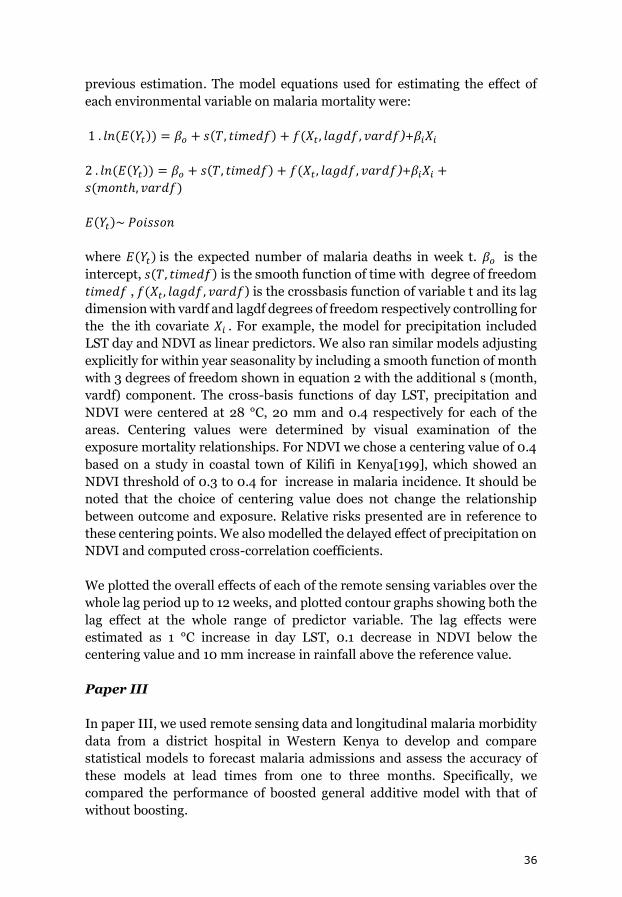
36

previous estimation. The model equations used for estimating the effect of

each environmental variable on malaria mortality were:

1 . 𝑙𝑛 (𝐸(𝑌𝑡)) = 𝛽𝑜 + 𝑠(𝑇, 𝑡𝑖𝑚𝑒𝑑𝑓) + 𝑓(𝑋𝑡 , 𝑙𝑎𝑔𝑑𝑓, 𝑣𝑎𝑟𝑑𝑓)+𝛽𝑖𝑋𝑖

2 . 𝑙𝑛 (𝐸(𝑌𝑡)) = 𝛽𝑜 + 𝑠(𝑇, 𝑡𝑖𝑚𝑒𝑑𝑓) + 𝑓(𝑋𝑡 , 𝑙𝑎𝑔𝑑𝑓, 𝑣𝑎𝑟𝑑𝑓)+𝛽𝑖𝑋𝑖 +

𝑠(𝑚𝑜𝑛𝑡ℎ, 𝑣𝑎𝑟𝑑𝑓)

𝐸(𝑌𝑡)~ 𝑃𝑜𝑖𝑠𝑠𝑜𝑛

where 𝐸(𝑌𝑡) is the expected number of malaria deaths in week t. 𝛽𝑜 is the

intercept, 𝑠(𝑇, 𝑡𝑖𝑚𝑒𝑑𝑓) is the smooth function of time with degree of freedom

𝑡𝑖𝑚𝑒𝑑𝑓 , 𝑓(𝑋𝑡 , 𝑙𝑎𝑔𝑑𝑓, 𝑣𝑎𝑟𝑑𝑓) is the crossbasis function of variable t and its lag

dimension with vardf and lagdf degrees of freedom respectively controlling for

the the ith covariate 𝑋𝑖 . For example, the model for precipitation included

LST day and NDVI as linear predictors. We also ran similar models adjusting

explicitly for within year seasonality by including a smooth function of month

with 3 degrees of freedom shown in equation 2 with the additional s (month,

vardf) component. The cross-basis functions of day LST, precipitation and

NDVI were centered at 28 °C, 20 mm and 0.4 respectively for each of the

areas. Centering values were determined by visual examination of the

exposure mortality relationships. For NDVI we chose a centering value of 0.4

based on a study in coastal town of Kilifi in Kenya[199], which showed an

NDVI threshold of 0.3 to 0.4 for increase in malaria incidence. It should be

noted that the choice of centering value does not change the relationship

between outcome and exposure. Relative risks presented are in reference to

these centering points. We also modelled the delayed effect of precipitation on

NDVI and computed cross-correlation coefficients.

We plotted the overall effects of each of the remote sensing variables over the

whole lag period up to 12 weeks, and plotted contour graphs showing both the

lag effect at the whole range of predictor variable. The lag effects were

estimated as 1 °C increase in day LST, 0.1 decrease in NDVI below the

centering value and 10 mm increase in rainfall above the reference value.

Paper III

In paper III, we used remote sensing data and longitudinal malaria morbidity

data from a district hospital in Western Kenya to develop and compare

statistical models to forecast malaria admissions and assess the accuracy of

these models at lead times from one to three months. Specifically, we

compared the performance of boosted general additive model with that of

without boosting.

37

In this study, we used malaria admissions data collected at the Siaya district

hospital for the period 2003-2013. The hospital surveillance data were

complete for this period and collected routinely by the health care workers

employed by the KEMRI/CDC. We extracted the admissions data for children

under five years of age with confirmed P. falciparum malaria. The data were

then aggregated to monthly time scale for each year to create a time series

dataset.

Satellite derived day and night LSTs, NDVI and precipitation data for the

period 2003-2013 were extracted and used as predictors. We averaged day

and night LSTs to get mean LST. In addition to these variables,

Evapotranspiration data from the MODIS product MOD16 available at 8 days

temporal and 1-kilometer spatial resolution was included. These datasets were

aggregated to monthly temporal resolution. We computed monthly totals for

rainfall and monthly averages for the other environmental factors.

A General Additive Modelling framework was employed to build forecast

models for malaria admissions, with smooth functions of environmental

factors at different lead times. Two different general additive models were

developed, one using a boosting algorithm to optimize model fit and the other

with no boosting. The malaria admissions data used in this study exhibited

over-dispersion. In a Poisson distribution, the mean and variance are equal.

Over-dispersion occurs when variance is greater than the mean. To account

for over-dispersion, we assumed negative binomial distribution in both

models.

The general additive model (GAM) without boosting was developed using the

mgcv package in R[194]. The model included a cubic regression spline of time

to adjust for the overall trend in malaria admissions during the study period.

To address the observed within-year seasonality of malaria, we used a cyclic

cubic regression function of month to capture the peaks in malaria

admissions. Mean LST, evapotranspiration (ET) and precipitation were

included as cubic regression splines in the model.

Malaria cases in any given month are likely to be correlated with malaria cases

in preceding months. The number of previously infected individuals

determines the reservoir of infectious mosquitoes, which in turn affects the

current population of infected individuals. To control for this autocorrelation,

we included previous malaria cases as autoregressive terms (AR) in the

models for each lead time. Previous studies in this HDSS area [21] and in

Burundi [200] included a 1-month AR term to adjust for autocorrelation. We

also included a simple random effect spline function of month. Smoothing

degrees of freedom were optimally determined using general cross validation.

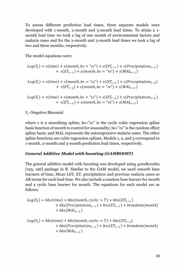
38

To assess different prediction lead times, three separate models were

developed with 1-month, 2-month and 3-month lead times. To attain a 1-

month lead time we took a lag of one month of environmental factors and

malaria cases and for the 2-month and 3-month lead times we took a lag of

two and three months, respectively.

The model equations were:

𝐿𝑜𝑔(𝑌𝑡) = 𝑠(𝑡𝑖𝑚𝑒) + 𝑠(𝑚𝑜𝑛𝑡ℎ, 𝑏𝑠 = "cc") + 𝑠(𝑙𝑆𝑇𝑡−1 ) + 𝑠(𝑃𝑟𝑒𝑐𝑖𝑝𝑖𝑡𝑎𝑡𝑖𝑜𝑛𝑡−1 )

+ 𝑠(𝐸𝑇𝑡−1 ) + 𝑠(𝑚𝑜𝑛𝑡ℎ, 𝑏𝑠 = "re") + 𝑠(𝑀𝐴𝐿𝑡−1 )

𝐿𝑜𝑔(𝑌𝑡) = 𝑠(𝑡𝑖𝑚𝑒) + 𝑠(𝑚𝑜𝑛𝑡ℎ, 𝑏𝑠 = "cc") + 𝑠(𝑙𝑆𝑇𝑡−2 ) + 𝑠(𝑃𝑟𝑒𝑐𝑖𝑝𝑖𝑡𝑎𝑡𝑖𝑜𝑛𝑡−2)

+ 𝑠(𝐸𝑇𝑡−2) + 𝑠(𝑚𝑜𝑛𝑡ℎ, 𝑏𝑠 = "re") + 𝑠(𝑀𝐴𝐿𝑡−2 )

𝐿𝑜𝑔(𝑌𝑡) = 𝑠(𝑡𝑖𝑚𝑒) + 𝑠(𝑚𝑜𝑛𝑡ℎ, 𝑏𝑠 = "cc") + 𝑠(𝑙𝑆𝑇𝑡−3 ) + 𝑠(𝑃𝑟𝑒𝑐𝑖𝑝𝑖𝑡𝑎𝑡𝑖𝑜𝑛𝑡−3 )

+ 𝑠(𝐸𝑇𝑡−3 ) + 𝑠(𝑚𝑜𝑛𝑡ℎ, 𝑏𝑠 = "re") + 𝑠(𝑀𝐴𝐿𝑡−3 )

𝑌𝑡~Negative Binomial

where s is a smoothing spline; bs=”cc” is the cyclic cubic regression spline

basis function of month to control for seasonality; bs=”re” is the random effect

spline basis; and MAL represents the autoregressive malaria cases. The other

spline functions are cubic regression splines. Models 1, 2, and 3 correspond to

1-month, 2-month and 3-month prediction lead times, respectively.

General Additive Model with boosting (GAMBOOST)

The general additive model with boosting was developed using gamBoostlss

[195, 196] package in R. Similar to the GAM model, we used smooth base

learners of time, Mean LST, ET, precipitation and previous malaria cases as

AR terms for each lead time. We also include a random base learner for month

and a cyclic base learner for month. The equations for each model are as

follows:

𝐿𝑜𝑔(𝑌𝑡) = 𝑏𝑏𝑠(𝑡𝑖𝑚𝑒) + 𝑏𝑏𝑠(𝑚𝑜𝑛𝑡ℎ, 𝑐𝑦𝑐𝑙𝑖𝑐 = 𝑇) + 𝑏𝑏𝑠(𝑙𝑆𝑇𝑡−1 )

+ 𝑏𝑏𝑠(𝑃𝑟𝑒𝑐𝑖𝑝𝑖𝑡𝑎𝑡𝑖𝑜𝑛𝑡−1 ) + 𝑏𝑠𝑠(𝐸𝑇𝑡−1 ) + 𝑏𝑟𝑎𝑛𝑑𝑜𝑚(𝑚𝑜𝑛𝑡ℎ)

+ 𝑏𝑏𝑠(𝑀𝐴𝐿𝑡−1 )

𝐿𝑜𝑔(𝑌𝑡) = 𝑏𝑏𝑠(𝑡𝑖𝑚𝑒) + 𝑏𝑏𝑠(𝑚𝑜𝑛𝑡ℎ, 𝑐𝑦𝑐𝑙𝑖𝑐 = 𝑇) + 𝑏𝑏𝑠(𝑙𝑆𝑇𝑡−2)

+ 𝑏𝑏𝑠(𝑃𝑟𝑒𝑐𝑖𝑝𝑖𝑡𝑎𝑡𝑖𝑜𝑛𝑡−2 ) + 𝑏𝑠𝑠(𝐸𝑇𝑡−2 ) + 𝑏𝑟𝑎𝑛𝑑𝑜𝑚(𝑚𝑜𝑛𝑡ℎ)

+ 𝑏𝑏𝑠(𝑀𝐴𝐿𝑡−2 )

39

𝐿𝑜𝑔(𝑌𝑡) = 𝑏𝑏𝑠(𝑡𝑖𝑚𝑒) + 𝑏𝑏𝑠(𝑚𝑜𝑛𝑡ℎ, 𝑐𝑦𝑐𝑙𝑖𝑐 = 𝑇) + 𝑏𝑏𝑠(𝑙𝑆𝑇𝑡−3 )

+ 𝑏𝑏𝑠(𝑃𝑟𝑒𝑐𝑖𝑝𝑖𝑡𝑎𝑡𝑖𝑜𝑛𝑡−3) + 𝑏𝑠𝑠(𝐸𝑇𝑡−3 ) + 𝑏𝑟𝑎𝑛𝑑𝑜𝑚(𝑚𝑜𝑛𝑡ℎ)

+ 𝑏𝑏𝑠(𝑀𝐴𝐿𝑡−3 )

𝑌𝑡~Negative Binomial

Where bbs is the smooth base learner. The smooth base learner for month is

set to be cyclic to control for seasonality. Random is the random base learner

for month. MAL represents the autoregressive malaria cases. Models 1, 2, and

3 correspond to 1-month, 2-month and 3-month prediction lead times,

respectively.

Model validation

To get an optimal number of boosting iterations we performed k-fold cross

validation on the training dataset. K-fold cross validation involves partitioning

the training data into k subsets. In each run, one subset is held for validation

while the remaining k-1 subsets are used for model fitting. The number of

iterations giving the lowest prediction in the k out of sample set is chosen.

We performed 5- fold validation with 1,000 initial iterations with 0·01 step to

get the number of boosting iterations for the gamboostlss model. To assess

the predictive ability of the models, we split the data into training and testing

datasets. The time series for the period 2003-2012 was used for model

training while the 2013-time series for model testing. R-squared statistic, root

mean squared error (RMSE), normalized mean squared error (NMSE), mean

absolute error (MAE) and normalized mean absolute error (NMAE) were used

for model comparison. The equations for these measures are given below:

𝑀𝐴𝐸 =1

𝑛∑ |𝑒𝑖|

𝑛

𝑖=1

𝑅𝑀𝑆𝐸 = √1

𝑛∑ 𝑒𝑖

2

𝑛

𝑖=1

𝑁𝑀𝑆𝐸 =1

�̅�√

1

𝑛∑ 𝑒𝑖

2,𝑛𝑖=1 where y̅ is the scaling factor

Where 𝑒𝑖 = 𝑓𝑖 − 𝑦𝑖 , where 𝑓𝑖 𝑖s the prediction and 𝑦𝑖 the observed value.

40

The NMAE is scaled using the lowest and the highest values in the series. The

different measures are relevant when there are different scales [201]; in this

case mean malaria admissions differ between test and training periods. These

measures have been explained in more detail in Shcherbakov et al [201]. We

included the normalized measures to be able to assess prediction accuracy

between training and test periods [201].All analysis was done using R

statistical software [202]. The DMwR [203] package was used to produce the

forecast accuracy statistics.

Paper IV

In this paper, we developed a framework to assess the economic value of an

operational early warning system to aid decision making within the public

health sector. The framework can be used to estimate the costs and benefits

associated with the use of early warning information generated by an EWS.

We proposed two different approaches on how forecasting can be integrated

into health systems for disease planning and response. The first method

assumes an early warning system that can issue alerts on high transmission

events based on disease thresholds while the other assumes a system that

churns out absolute disease forecasts.

Decision-analytical modelling framework [204, 205] was the quantitative

approach proposed for assessing costs and benefits incorporating the accuracy

of disease forecasts. We defined economic value as net benefit, which is total

benefits minus total costs. A positive net benefit is a general signal to policy

makers that response measures are economically feasible. In principle, the

probability of a false warning in the case where threshold is used or prediction

errors decreases as the lead time decreases. However, shorter lead times may

mean reduced cost savings due to reduced amount of averted disease burden.

The proposed framework makes it explicit the trade-offs between forecast

accuracy, cost of response, and potential cost savings as a function of lead

time.

41

Results

Distribution of malaria health outcomes

Mortality

Between 2003 and 2008, 1768 malaria deaths occurred among children under

the age of five in Asembo and Gem areas of the KEMRI/CDC HDSS. Physician

coding was employed to derive cause of death from VA questionnaires. There

was an average of 5.6 malaria child deaths in a week. Between 2003 and 2006,

there was a steady decline in the number of child deaths due to malaria, but

the trend reversed in 2008. The highest number of deaths (386) was observed

in 2004 with 2008 following closely at 368 deaths. A general seasonal pattern

was observed and is captured in Figure 11. The highest average monthly

number of admissions occurred in May while October registered the least

number of admissions. The number of malaria mortality events derived using

probabilistic INTERVA method for VA between 2003 and 2012 in all the three

HDSS areas was 3,809. The highest number total malaria deaths in a year was

696 observed in 2008. The least number of deaths was observed in 2007 with

210 malaria deaths. The average weekly malaria deaths were 2 and weekly

average deaths ranged from 0 to 20 deaths.

Malaria admissions

There were 8,476 confirmed P. falciparum malaria admissions for children

under the age of five at Siaya district hospital between 2003 and 2013 with a

mean of 64 admissions due to malaria per month. The years 2003, 2004 and

2008 saw the highest number of admissions with 1258, 1468 and 1249

respectively. There have been huge declines in admissions over the years with

the recent years registering very low number at 197 and 166 admissions for the

years 2012 and 2013.

Distribution of weather variables

Temperature

From the Kisumu airport data, the mean temperature for the entire period

2003-2008 was 23.6C and ranging from a minimum of 20.7C to a maximum

of 27.6C. The hottest years recorded was 2005 with a mean temperature of

24.1C. The maximum temperature ranged from 25.4 to 35.5C with a mean

of 29.5C in the same period while the minimum temperature varied between

14.4 and 20.8C. For the period 2003 to 2012, the day land surface

42

temperature from MODIS for the entire KEMRI/HDSS area ranged from

19.9C to 39.1C with a mean of 29.7C. In terms of regional differences in day

LST, the mean day LST for Asembo, Gem and Karemo for the entire study

period 2003-2012 was 30.5C, 29.1C and 29.4C respectively. The time series

of the distribution of temperature in Kisumu is captured in Figure 10.

Precipitation

The rainfall data summaries for Kisumu show that the average total weekly

rainfall amounts are 23 mm and range between 0-232 mm. The total rainfall

observed between 2003 and 2008 in Kisumu was 7,446 mm. The wettest year

was 2006 with a total rainfall of 1,548 mm and the driest year was 2005 with

total rainfall of 969 mm with a mean of 18.3 mm per week (refer to Figure 10).

The average total precipitation registered in the three KEMRI/CDC HDSS

areas for the whole period 2003 to 2012 was 15,609 mm with a mean weekly

precipitation of 29.5 mm with a maximum of 196 mm. Similar to Kisumu the

wettest year in the HDSS areas was 2006 with a total rainfall of 2,172 mm and

2005 as the driest year with total rainfall of 1,343 mm. Comparing the three

HDSS areas, Gem received the highest amount of rainfall in the period 2003

to 2012 with total rainfall of 16,541 mm followed by Karemo at 15,683 mm and

finally Asembo with 14,602 mm of rainfall. The average weekly total rainfall

in Asembo was 27.6 mm, 31.2 mm in Gem and 29.6 mm in Karemo.

Normalized difference vegetation index (NDVI)

For all the three HDSS areas, the weekly mean NDVI was 0.61 and ranged

from 0.3 to 0.77 in the period 2003 to 2012. The highest mean NDVI was in

2007 at 0.65 while the least mean NDVI was in 2009 with a value of 0.58. Gem

region is the greenest with a mean NDVI of 0.64 followed by Karemo with an

NDVI of 0.62 and the least green being Asembo with mean NDVI of 0.58. In

2007, the greenest year, all the three areas registered mean NDVI values above

0.6. The distribution is displayed in Figure 10.

43

Figure 10. Time of series plot of weather data (mean temperature, min temperature,

maximum temperature and precipitation(KIS)) from Kisumu airport 2003-2008 and remote

sensing 2003-2012. Day LST, precipitation (TRMM) and NDVI are satellite derived and the rest

from the airport. The plot also describes malaria deaths by INTERVA and physician coding

cause of death derivation.

44

Figure 11. Weekly seasonal distribution of malaria deaths and remote sensing derived day LST,

NDVI and precipitation in three endemic areas Asembo, Gem and Karemo, Western Kenya

aggregated for the period 2003-2012.

Seasonality of malaria deaths and environmental variables

Figure 11. Shows weekly mean malaria mortality plotted against weekly

summaries of remote sensing variables. We can see clearly that peaks in

malaria mortality follows peaks of environmental factors with different lag

phase shifts. Figure 12 shows the within year weekly distribution of malaria

mortality, day LST, precipitation and NDVI contrasted by area while Figure

13 shows monthly distribution of malaria admissions. We observe two peaks

in malaria transmission corresponding to the bimodal peaks also observed for

the environmental variables. Malaria mortality increases gradually from

about week 12 and peaks at week 22 and another less peak occurs towards the

end of the year starting from week 42 and peaking at week 48. The peak in day

LST occurs during the weeks of February. The increase in precipitation starts

from week 9 and peaks at week 19 and again start at week 39. The two peaks

for NDVI are at 19 and 46 weeks respectively.

45

Figure 12. Weekly seasonal distribution of malaria deaths and remote sensing derived day LST,

NDVI and precipitation by KEMRI/CDC HDSS area 2003-2012.

Figure 13. Average monthly admissions of under 5 P falciparum malaria cases at Siaya district

hospital 2003 -2013.

46

Relationship between environmental factors and malaria mortality

Mean temperature

Figure 14 shows association between weekly malaria mortality in Asembo and

Gem and mean weekly temperature from Kisumu airport at different lag

strata. There is no significant relationship for lag strata derived from week 1

to week 8. The exposure lag response relationship changes for longer lags from

9 weeks. At lag strata of 9-12 weeks, the relative risk is significant at

temperatures of above 25 and increases almost linearly. The lag effect is

stronger for mean temperatures above 25C at lag 13-16 weeks.

Figure 14. Relative risks of Malaria/Anemia mortality in children under five years with weekly

mean temperature (Tmp) at different lag strata [59].

47

Day land surface temperature

Figure 16A shows the overall effect of day LST on weekly malaria mortality in

Asembo, Gem and Karemo areas combined over the whole lag period. The

effect of day LST is significant for temperatures above 34C compared to the

reference of 29C. For example, at day LST of 36.9C the relative risk of

malaria mortality is 2.19 [1.29-3.74]. When we compare the overall effect by

study area we observe some differences as displayed in Figure 17. In Asembo

Figure 17A, there is no significant LST value across the range of LST. However,

in Gem, Figure 17D; there is a significant risk association for day LST below

27C and above 34C. For example, at 24.9C the RR is 1.66 [1.02-2.73] and

for LST of 36.9C the RR is 3.23 [1.59-6.56] resulting in a U-shape typical of

temperature mortality relationships. In karemo Figure 17G the effect is

significant for lower temperature e.g. at LST of 25.7 the RR is 2.06 [1.26-3.37].

Delayed effect of day LST

Figure 16D shows the exposure lag response relationship between day LST

and malaria mortality in all the three areas combined in a contour plot. We

observe shorter lag positive significant effect at lower day LST values below

29C and longer lag effect for LST values in the upper percentiles. Figure 18

displays this lag pattern for specific weekly day LST values. In Figure 18, we

see that for weekly LST value of 27.3C, the lag effect is significant from lag

week 0 to lag week 4. At lag week 4, the RR is 1.0086 [1.003-1.014]. At higher

weekly day LST of 36.9C the lags are significant from lag week 7 up to lag

week 12 with highest relative risk at week 12 amounting to 1.23 [1.09-1.4].

Precipitation

Figure 15 shows the exposure-response relationship as lag strata between

weekly cumulative precipitation from Kisumu airport and under five malaria

mortality in Asembo and Gem for the period 2003 to 2008. There is no

significant effect at combined lags 1 to 4 weeks. There is relatively increased

risk for weekly total rainfall between 120 mm and 180 mm in lag strata 5 to 8

weeks. However, the relationship is stronger for lags 9 to 12 weeks with linear

increase in risk with increasing weekly total rainfall. With higher lag 13-16

weeks the risk increase from 80 mm and then starts to drop at 200 mm

resulting in an inverted U-shaped relationship.

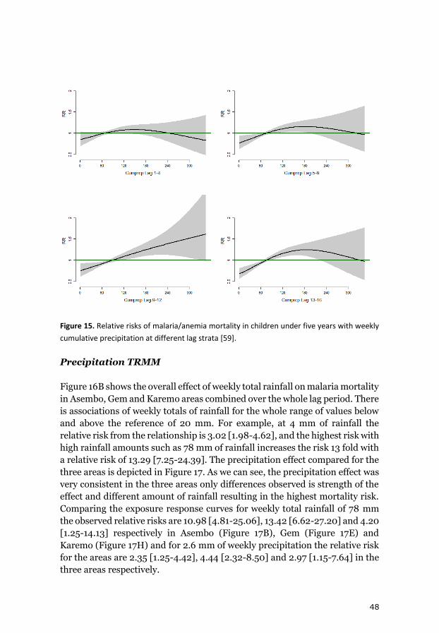
48

Figure 15. Relative risks of malaria/anemia mortality in children under five years with weekly

cumulative precipitation at different lag strata [59].

Precipitation TRMM

Figure 16B shows the overall effect of weekly total rainfall on malaria mortality

in Asembo, Gem and Karemo areas combined over the whole lag period. There

is associations of weekly totals of rainfall for the whole range of values below

and above the reference of 20 mm. For example, at 4 mm of rainfall the

relative risk from the relationship is 3.02 [1.98-4.62], and the highest risk with

high rainfall amounts such as 78 mm of rainfall increases the risk 13 fold with

a relative risk of 13.29 [7.25-24.39]. The precipitation effect compared for the

three areas is depicted in Figure 17. As we can see, the precipitation effect was

very consistent in the three areas only differences observed is strength of the

effect and different amount of rainfall resulting in the highest mortality risk.

Comparing the exposure response curves for weekly total rainfall of 78 mm

the observed relative risks are 10.98 [4.81-25.06], 13.42 [6.62-27.20] and 4.20

[1.25-14.13] respectively in Asembo (Figure 17B), Gem (Figure 17E) and

Karemo (Figure 17H) and for 2.6 mm of weekly precipitation the relative risk

for the areas are 2.35 [1.25-4.42], 4.44 [2.32-8.50] and 2.97 [1.15-7.64] in the

three areas respectively.

49

Delayed effect of precipitation

The contour plot in Figure 16E shows the lag patterns at different values across

the range of weekly total rainfall. For weeks with total precipitation below 20

mm, the lag effect is delayed significant increased risk from week 5 and for

weeks with higher cumulative rainfall, the lag effects are immediate starting

at week 0. At lag week 1 and 8, the relative risk for mortality are 1.18 [1.08-

1.28] and 1.30 [1.21-1.39] for 78 mm of rainfall. At 9 mm of weekly rainfall the

first significant lag is week 6 with an RR of 1.06 [1.001-1.11] and the risk

increase for each subsequent lag with highest risk at lag 12 with RR of 1.11

[1.06-1.15]. This lag relationship for precipitation is captured in Figure 18.

Normalized difference vegetation index (NDVI)

Figure 16C shows the overall effect of average weekly vegetation index on

malaria mortality in Asembo, Gem and Karemo areas combined over the

whole lag period. The risk is higher for weeks with vegetation indices below

0.4, which is the reference value. For example, at NDVI values 0.3 and 0.2 the

relative risks for mortality increases by 3.10 [1.73-5.56] and 9.62 [2.99-30.94]

respectively. The risk for malaria death is significantly lowered with higher

NDVI values, e.g. for weeks with average NDVI of 0.62 the relative risk is 0.28

[0.16-0.48]. Exploring the association considering area offers some

differences between the study areas. At weekly average of NDVI of 0.3 the RR

risks in Asembo (Figure 17C), Gem (Figure 17F), are 2.18 [1.06-4.51] and 3.40

[1.64-7.05], but not significant in Karemo (Figure 17I) with a relative risk of

1.45 [0.44-4.83].

Delayed effect of NDVI

The temporal relationship between NDVI and malaria mortality is displayed

as a contour plot in Figure 16F.From the contour plot, we see that with NDVI

below 0.4, the lag effect has a strong effect at short lags, while at high indices

the effect is more delayed and protective. Figure 18 shows risk of malaria

deaths at different lag weeks for specific values of NDVI. For weeks with

average NDVI of 0.3, the lag effect is stronger at lag 0 and significant up to

week 5 with a decreasing trend. For example, at lag week 1 the RR is 1.16 [1.05-

1.28] and 1.07 [1.004-1.15] at lag week 5. Very vegetation green weeks with

NDVI of 0.7 reduces the risk of malaria death at longer lags, e.g. a RR of 0.89

[0.82-0.97] for a lag of 10 weeks.

50

Figure 16. The overall risk of day Land Surface Temperature (LST oC) (A), precipitation (mm)

(B), and Normalized Difference Vegetation Index (NDVI) (C) on malaria mortality for all areas

for the whole lag period. The bold lines indicate relative risks while the shaded regions display

the 95% Confidence intervals. D, E and F are the lag patterns for day LST, precipitation and

NDVI respectively at the whole range of predictors [60].

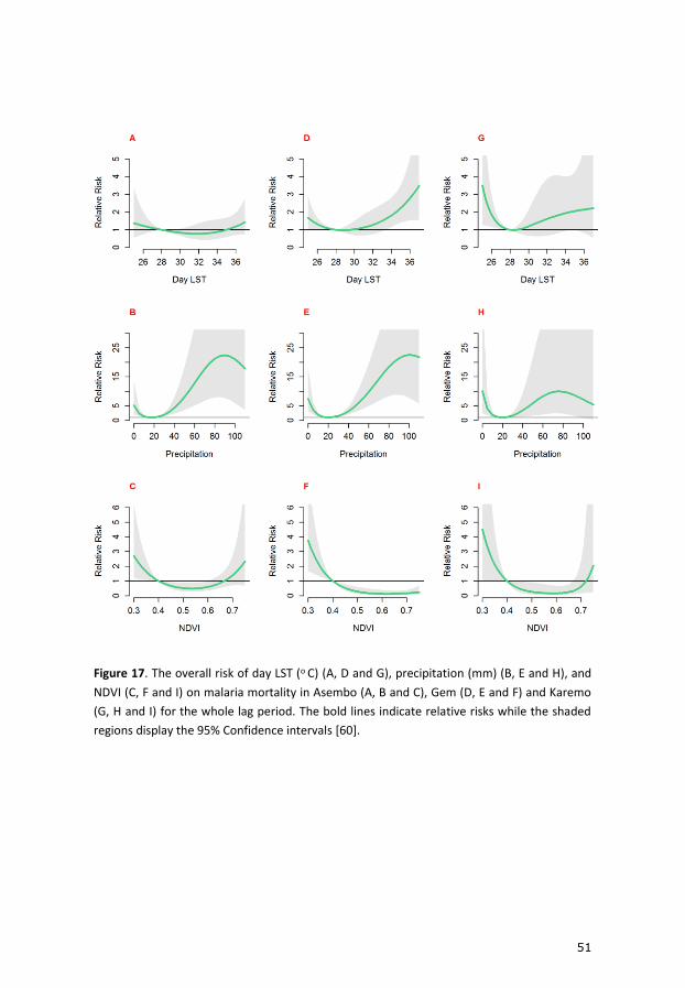
51

Figure 17. The overall risk of day LST (o C) (A, D and G), precipitation (mm) (B, E and H), and

NDVI (C, F and I) on malaria mortality in Asembo (A, B and C), Gem (D, E and F) and Karemo

(G, H and I) for the whole lag period. The bold lines indicate relative risks while the shaded

regions display the 95% Confidence intervals [60].

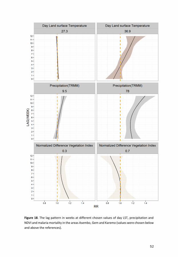
52

Figure 18. The lag pattern in weeks at different chosen values of day LST, precipitation and

NDVI and malaria mortality in the areas Asembo, Gem and Karemo (values were chosen below

and above the references).

53

Prediction of monthly malaria admissions

Table 1 shows various model prediction metrics comparing GAM modelling

approach and the GAMBOOST approach at different prediction lead times

ranging from 1 to 3 months in forecasting malaria admissions among children

at the Siaya district hospital. The GAM model with boosting performed better

at all the prediction lead times. The most accurate lead time was one month

in all the models. For the 1-month lead time, the GAMBOOST model explained

80% of the variation in the data during training period 2003-2012 and 71% of

the variation in the forecasting of 2013 malaria admissions. The GAM model

at 1-month lead time captures 77% of the variation during training, but was

not able to replicate this during forecasting of the 2013 cases. With increasing

lead times, the predictive capability of both models decreased. For example,

the GAMBOOST model only accounted for 50% of the variation at the 3-

month lag internal prediction.

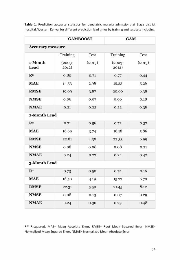
54

Table 1. Prediction accuarcy statistics for paediatric malaria admissions at Siaya district

hospital, Western Kenya, for different prediction lead times by training and test sets including.

GAMBOOST GAM

Accuracy measure

1-Month

Lead

Training

(2003-

2012)

Test

(2013)

Training

(2003-

2012)

Test

(2013)

R2 0.80 0.71 0.77 0.44

MAE 14.53 2.98 15.33 5.26

RMSE 19.09 3.87 20.06 6.38

NMSE 0.06 0.07 0.06 0.18

NMAE 0.21 0.22 0.22 0.38

2-Month Lead

R2 0.71 0.56 0.72 0.37

MAE 16.69 3.74 16.18 5.86

RMSE 22.81 4.38 22.33 6.99

NMSE 0.08 0.08 0.08 0.21

NMAE 0.24 0.27 0.24 0.42

3-Month Lead

R2 0.73 0.50 0.74 0.16

MAE 16.50 4.19 15.77 6.70

RMSE 22.31 5.50 21.45 8.12

NMSE 0.08 0.13 0.07 0.29

NMAE 0.24 0.30 0.23 0.48

R2= R-squared, MAE= Mean Absolute Error, RMSE= Root Mean Squared Error, NMSE=

Normalized Mean Squared Error, NMAE= Normalized Mean Absolute Error

55

Figure 19. Observed and predicted paediatric malaria admissions at Siaya district hospital,

Western Kenya by prediction lead time for the period 2003-2013 from the GAMBOOST model.

The black line displays observed malaria admissions, the grey line predicted values during the

training period 2003-2012, and the red line the 2013 forecasted values. The red vertical dotted

line marks the beginning of the test period.

The normalized mean squared error (NMSE) is very comparable in

GAMBOOST 1-month lead time with 0.06 and 0.07 during model training and

testing periods respectively. Thus, the model validation reinforce the

GAMBOOST algorithm to provide better predictive power comparing to the

GAM model. Figure 19 shows a graphical, comparison between observed

malaria admissions data and the model predictions. The GAMBOOST model

capture closely the yearly seasonal pattern and the peak closely for the 1-

month lead time model.

56

A framework for economic evaluation of early warning and response system benefits

Options to health system integration

This framework outlines two different approaches on how forecasting can be

integrated into the health systems: 1. We assume an existing operational early

warning system capable of issuing forecast of high/epidemic events several

months ahead at discrete intervals. In this situation we predict the probability

of exceeding the pre-defined threshold, e.g. P(�̂�𝑡>threshold) where �̂�is the

number of cases or incidence (approach 1); or, 2 we assume integration of

forecasting within existing surveillance systems as a routine activity and

predict the number of cases, or incidence, �̂�𝑡 (approach 2). In the situation the

health outcome, �̂�𝑡, is a number of disease counts, we can estimate the number

of cases that require hospitalization, the number of cases that progress to

severe disease and the number of deaths. On the cost side, both methods

include the actual costs of response strategies at different lead times, but the

first approach also includes the costs of false (positive or negative) warnings

given the forecast accuracy. On the benefits side, we include the valuation of

averted health outcomes (averted disease burden in terms of uncomplicated

and severe cases) in monetary units given the level of uncertainty associated

with disease forecasts and the effectiveness of response strategies at different

lead times.

Uncertainty of forecasts

There are a few key characteristics of a disease forecast. An important one is

that with increasing forecasting lead time, i.e. the time for issuing of forecast

to the realization of forecast, the accuracy of detecting epidemic intensity, is

expected to diminish. For the forecasted entity �̂�𝑡 (approach 2), we estimate

the validity of the forecast by measuring the mean square error (MSE) of the

prediction to the true occurrence of the disease. In approach 2, where the

predicted entity is P(�̂�𝑡>threshold), we estimate the accuracy of detecting this

anomalies beyond the threshold by the forecast as a probability.

Response interventions

For forecast of disease frequencies, or epidemics, becoming useful within the

health system, they need to be aligned to a set of response strategies. The

longer lead time is considered an attractive feature in preparing and

responding to future disease events, where possibilities are given to extend the

routine surveillance activities and to make them more rigorous. The lead time

can also open up for new possibilities of intervening and preventing, or

57

limiting the impact, of outbreaks, and potentially make the effect of response

activities stronger. In this research, we assume decision makers have already

a set of interventions known to be effective in preventing disease, of which

they also know how much time they need in the implementation to reach this

effect, so that they can synchronize this with a response at a specific lead time.

We symbolize the relationship between intervention effectiveness and lead

time using, 𝑒𝑖 where e denotes the effectiveness of the specific intervention, or

for a combination set of interventions (e.g. a response program), and where i

denotes the lead time.

Costs of disease management, information management, and

response programs

The cost components include the cost of response programs for each

intervention, or combinations of interventions, e.g. the cost of running a

response program at a specific lead time and the cost of running the

information management system, which we assume constant. We denote CRi

as the cost of the response at lead time i, the while the cost of information

management is denoted CI. We assume that the costs of interventions in the

response program is known, and ultimately, for each lead time decision

makers have identified a set of response action to take given their operational

capacity and estimated how much the cost is for running the program to

achieve the desired effect. We also assume the cost of running the forecasts

and dissemination information, CI, is known.

We further consider the direct medical costs of outpatient and inpatient

treatment of cases in the formal health sector, and denote this with CT. Thus,

we consider the economic burden of disease will be measured using the cost

of treatment, but the cost of hospitalizations and management of severe

disease can be used. CT can be used as an entity providing an economic

valuation of each specific averted disease case from the response activities. We

assume that models estimating the probability of epidemics still can provide

estimates of disease cases and hospitalizations associated with the predicted

event. In the latter case, the disease frequency estimates are considered the

excess numbers beyond the specified acceptance threshold.

Net benefit of response programs

To assess the economic value of a response program, we formulate an

equation for estimating the net benefit of responding to the forecasted disease

frequency or epidemic. We define the net benefit as 𝑁𝐵𝑡,𝑖, where t denoted

time and i denotes lead time. We set up two different ways to quantify the net

benefits, one for the situation where the threshold is pre-defined and we

58

estimate the outbreak probability and excess morbidity/mortality (approach

1), the other where we forecast the morbidity and evaluate the net benefit of

responding (approach 2). In situations where the threshold for epidemics is

defined and �̂�𝑡 predicts excess beyond this threshold, we defined 𝑁𝐵𝑡,𝑖 as

function of:

𝑁𝐵𝑡,𝑖 = (�̂�𝑡,𝑖 ∗ 𝑒𝑖 ∗ 𝐶𝑇) − (𝐶𝐼 + 𝐶𝑅𝑖 + (𝑃𝑓𝑎,𝑖 ∗ 𝐶𝑅𝑖)) (1)

Here �̂�𝑡,𝑖 ∗ 𝑒𝑖 represents cases averted due to the response at lead time i, and

𝑃𝑓𝑎,𝑖 ∗ 𝐶𝑅𝑖 is the cost of false alarm at lead time i. Thus, the cost of intervening

is weighted using the probability of false alarm. To this, we add the running

costs, CI, and the value of each averted case, CT.

In situations where the threshold for epidemics is not defined and �̂�𝑡 predicts

total cases, we define 𝑁𝐵𝑡,𝑖 as:

𝑁𝐵𝑡,𝑖 = (�̂�𝑡,𝑖 ∗ 𝑒𝑖 ∗ 𝐶𝑇) − (𝐶𝐼 + 𝐶𝑅𝑖) (2)

Here, there is no false-alarm penalization, but the �̂�𝑡,𝑖 will instead be including

the MSE of forecasted to observed differences, which is going to be larger if

the forecasts are “missing” epidemics. The other parameters are similar to

those described in formula (1).

Simulation of uncertainty

The parameters used in the formula for computing net benefits have

uncertainty around them. Sensitivity analysis can be used to show the changes

in net benefit as the parameters are varied. Due many parameters with

uncertainty, we propose to use probability sensitivity analysis (PSA) to model

the uncertainty around the parameters. The uncertainties are assumed to

follow probability distribution functions. The uncertainty around forecast

prediction, intervention effectiveness, and probability of false alarms can be

assumed to follow a Poisson/binomial, Asymptomatic normal and binomial

distributions, respectively, while the uncertainty around costs may be

assumed to follow lognormal or uniform distributions. Markov Chain Monte

Carlo (MCMC) simulation can then be used to draw several samples

randomly, for example 10,000 samples, based on the probability distribution

of the model parameters in the formulas (1) and (2) resulting in a simulated

estimated of the distribution of 𝑁𝐵𝑡,𝑖. The estimated probability distribution

function of 𝑁𝐵𝑡,𝑖 can be computed at each time t and for each lead time i. We

illustrate a hypothetical distribution of 𝑁𝐵𝑡,𝑖 in Figure 20.

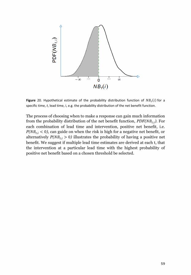
59

Figure 20. Hypothetical estimate of the probability distribution function of 𝑁𝐵𝑡(𝑖) for a

specific time, t, lead time, i, e.g. the probability distribution of the net benefit function.

The process of choosing when to make a response can gain much information

from the probability distribution of the net benefit function, PDF(𝑁𝐵𝑡,𝑖). For

each combination of lead time and intervention, positive net benefit, i.e.

P(𝑁𝐵𝑡,𝑖 < 0), can guide on when the risk is high for a negative net benefit, or

alternatively P(𝑁𝐵𝑡,𝑖 > 0) illustrates the probability of having a positive net

benefit. We suggest if multiple lead time estimates are derived at each t, that

the intervention at a particular lead time with the highest probability of

positive net benefit based on a chosen threshold be selected.

60

Discussion

In order to develop effective malaria early warning programs, the need to

quantify the relationship between environmental factors such as rainfall and

temperature with malaria burden becomes apparent. The relationship

between these factors in the environment and malaria is expected to follow

biological progression with varying temporal delay between exposure and the

event. This temporal dimension provides useful information that can guide

the timing of interventions to curb the devastating effects such in epidemic

situations. In this thesis, we have made effort to answer specific questions

regarding the presence of interacting weather factors, remote sensing proxies

for changes in environmental conditions and malaria mortality in rural

western Kenya using state of the art modelling techniques and used the

information to develop predictive models that can be used in early warning

situations.

In the first objective, we explored the lagged relationship between weekly total

rainfall, weekly mean temperature and malaria mortality for Asembo and Gem

areas of the KEMRI/CDC HDSS combined using general additive modelling

framework that allowed us to model the weather covariates as smooth

functions. For example, we have shown that the effect of mean temperature

on malaria mortality is much delayed starting to manifest from week 9 with

linear increase with average temperatures above 25oC, and a J-shaped

relationship with lags greater than 13 weeks. These results echo with lag

patterns identified by Chirebvu et al in Botswana where they found a positive

correlation between malaria transmission and maximum temperature with a

lag of 2 months and a lag of one month for mean temperature [206]. However,

in this study they assume, linear relationship between temperature and

malaria transmission. A recent study that employed general additive mixed

model to tease out the relationship between air temperature and malaria

incidence in Uganda and Rwanda using spline functions, reported positive

relationship between air temperature with malaria incidence with a lag

ranging from zero to 2 months in Rwanda and quadratic relationship between

temperature and malaria incidence in Uganda with protective effect for

temperatures below 30oC in Uganda [207]. Some studies have looked at the

effect of temperature and malaria without considering the lag dimension. For

example, in Nepal, an increase by 1 degree in mean temperature resulted in a

25% increase in risk of malaria [208]. In Papua New Guinea [209] a positive

association was observed for min temperature between 0-2 months, which

resonates with our findings for Asembo, and Gem. However is some regions,

like Chennai in India, shorter lag of 1 month was observed between malaria

and temperature [210]. Using a mathematical model to simulate the effect of

61

temperature on malaria incidence, an optimal temperature of between 21-25

oC was needed for maximum malaria transmission in Kwazulu Natal region in

south Africa [211], in our study region the effect of temperature is seen for

weeks with mean temperatures above 24oC.

Land surface temperature

In the second objective, we assessed the relationship between variables

derived by satellites and their relationship with malaria mortality in all the

three areas of the KEMRI/CDC HDSS. For temperature we used the MODIS

derived day land surface temperature as a proxy for surface temperature. At a

spatial resolution of 1km, we could assess the spatial differences in

relationship between the regions. In the second objective, we use distributed

lag non-linear models, which permitted simultaneous modelling of both the

lag and exposure space. For Asembo, Gem and Karemo areas combined, there

was an increase in risk for day LST above 34oC and a decrease in risk for day

LST from minimum to 28oC. We observed negative relationship shown by

decreasing risk with day LST below 29oC from week 0 to week 4 which is

similar study in the HDSS that showed negative relationship between day LST

and malaria transmission with a lag of 1 month [21] and in as study by Hay

Kilifi [57]. In the study by Hay [57]on the effect of day LST on malaria

admissions, they did not find any correlation In Siaya district but we show

positive relationship with day LST below 29oC. Day LST has been shown to

associate with mosquito density for period of between current and previous

month in Nouna HDSS in Burkina Farso [212].

Several other studies have used the flexible DLNM approach as we did to study

the effect of weather factors and malaria incidence [213-218]. Others have

used polynomial distributed lag model [219, 220], which is similar to DLNM

framework as it imposes constraints on the coefficients which reduces the

model degree of freedom. For example, using DLNM [213] in China, it was

shown that 1-degree increase in min temperature was significant for lags 4 to

9 weeks with highest risk at 7 weeks. This close to what we find of delayed lag

effect for day LST above 29oC which was the reference from week 7. Again, in

China, Guo [214] showed that high temperatures were associated with

increased risk of malaria with effect lasting 4 weeks for temperatures above

30oC, which is similar to our reference temperature of 29oC when constructing

the cross basis function in the DLNM. In Ethiopia[81], a positive association

was found between 1 month lag of LST and malaria incidence. In endemic

regions of Zambia a quadratic relationship between day LST was identified,

the risk increased with day LST above 30oC, which quite similar with what we

find with our analysis [221]. In areas stratified as hot in Ethiopia, max

temperature was found negatively associated with malaria incidence with

62

shorter lags of 3, 4 and 5 weeks [219]. In the Kenyan coast [220], max

temperature was shown to associate negatively with malaria incidence

between 5-35 days and positively associate with max temperature from 29-48

days which echoes our finding of longer lag effects for higher day LST.

Precipitation

For both the first and second paper, the effect of precipitation showed

nonlinear relationship, where the risk for malaria mortality increased linearly,

then decreased after reaching various thresholds. In the first objective, the

effect of total rainfall started manifesting after lag of 5 weeks, with effect

showing more strongly after lag of 9 weeks with linear relationship and at

longer lags, 13 to 16 weeks the effect showed the regular inverted U-shaped

relationship. At 13-16 weeks’ lag, the threshold is about, 140 mm/week of

rainfall after which the mortality relationship declines. This nonlinear

relationship between precipitation has been shown in other studies, for

example in Botswana [69] a quadratic relationship was found, with the

relationship forming the basis of a predictive model for early warning. When

they included 0 to 2 months lag of rainfall in a spatio-temporal model, Amek

et al. did not any relationship between rainfall and malaria transmission [21].

This could be due to several reasons, the inclusion of NDVI, which is a proxy

for water content, and probably the assumption of linearity between rainfall

and malaria transmission. In another study in the HDSS [24]areas, previous

total annual rainfall also did not any effect on malaria mortality and may due

consideration of longer lag ranges and assumption of linearity masking the

true relationship. A study in Nepal that did not take into account lags of

monthly total rainfall and included relative humidity also did not find any

relationship between rainfall and malaria risk [208].

In the second paper, we showed the relationship between TRMM satellite

precipitation and malaria mortality in the three areas in the KEMRI/CDC

using DLNM to capture both the lag and exposure space. The relationship

again was well captured by smooth cubic splines where the mortality risk

increased from a weekly total precipitation of 20 mm, then peaked at about a

weekly total of 80 mm of rainfall, and then declined. The threshold, the point

of maximum mortality in this analysis at 80 mm of weekly rainfall was

different for the first paper. This may be due to differences in source of rainfall

data. The TRMM rainfall data was extracted for the HDSS study area while in

paper 1 we used rainfall data collected at Kisumu airport, which is about 60

km away and may not have represented the precipitation patterns in the study

area. This underscores the importance of remote sensing data in improving

risk assessment in geographic areas where routine collection of weather data

may be lacking. Using DLNM, it has been shown that 10 mm increase in

63

rainfall increased the risk of malaria at lags of 2-4 weeks and 9-10 weeks with

highest risk at week 3 in china [213]. In our analysis a similar observation is

noted, where higher total weekly rainfall having short lag effect with effect

starting from week 0. The study in Rwanda and Uganda [207], where they

modelled rainfall and malaria incidence using DLNM, with mathematical

simulation in kwazulu Natal [211] and semiparametric Poisson regression in

endemic areas in Zambia [221], showed a similar relationship, where there is

increase and then decrease, resulting in an inverted U-shaped relationship as

we have similarly shown. In kwazulu Natal, precipitation effect peaked at 107

mm of rainfall and then declined [211] while in Zambia [221] it peaked at 100

mm of total rainfall. However, in Guangdong in China [214], a J-shaped

relationship was found between rainfall and malaria incidence with a

threshold of 150 mm of weekly total rainfall and effect precipitation

manifesting after 4 weeks and persisting for 15 weeks. They identified a high

risk at week 8 with 225 mm of total weekly rainfall. In some studies in Kenya,

along the coastal region and western Kenya at Siaya [199] , a longer lag of 2

months was identified for cold cloud duration and malaria admissions in

Kenya, which is a proxy for rainfall and in Sudan[222] a 2 month lag of rainfall

was associated with density of An arabiensis. In Guinea, the lag relationship

between rainfall and malaria differed in the region studied with a range of 1-

2 months [209]. In Niger using the DLNM approach [215], the delayed effect

of 1 mm increase in rainfall resulted in 7.2% increase in risk with highest risk

observed between 32 and 33 days. In Ghana, the delayed effect was evident

between 1 – 2 weeks and 9 weeks in endemic regions [223]. A study in

highlands of Ethiopia showed that TRMM precipitation products performed

better as explanatory variable to malaria occurrence than other products and

had positive relationship with malaria disease with a lag of 1-3 months [81].

In Ethiopia [219], using polynomial distributed lag method, the effect of

rainfall was positive at lags of 10-12 weeks with maximum lag at 12 weeks in

areas that were classified as cold. In this study, regions that were classified as

hot had shorter lag effects for rainfall from 6 weeks persisting to week 10.

Using the same method as above, it was shown that rainfall was associated

with mosquito density between 4-47 days in coastal regions of Kenya [220].

Normalized difference vegetation index

In the second paper, in addition to day LST and precipitation, we also

modelled the relationship between mean weekly NDVI values and malaria

mortality. We observe an L-shaped relationship. Mortality risk is higher for

NDVI of below 0.4 and protective for NDVI above 0.4. This threshold of

between 0.3 and 0.4 has been shown between NDVI and malaria admissions

in Kilifi in the coast and Siaya district in Western Kenya. For example in Siaya,

the correlation was 0.6 with a 1-month lag [57]. The L-shape relationship is

64

consistent in the three areas, Asembo, Gem and Karemo. The lag pattern is

similar to what we show and with NDVI below 0.4; the lag association is

significant from week 0 to week 5. Amek, [21] showed that NDVI was

positively related with mosquito density in Asembo and Gem; however they

did not show the NDVI ranges that are significant. Midekisa also showed the

NDVI had a lag of 1-3 month with malaria incidence in Ethiopian highlands

[81]. The interaction between NDVI and rainfall could explain the difference

in expected increase in risk with increasing NDVI. However, we observe that

for lower NDVI, below 0.4 the risk increased. One explanation for this could

be that, when NDVI is low, it means the conditions are drier and any pools of

water may provide suitable breeding sites for mosquitoes thus increase in risk

while when the NDVI is above, 0.4 there could be presence of more water

related to high rainfall amounts which could result in the flushing away of

mosquito breeding sites resulting in the protective effect observed in our

study.

Prediction of malaria admissions

After the lag and risk assessment in objective 1 and objective 2, we used the

information to develop predictive models for P. falciparum malaria

admissions for children using lagged remote sensing data to provide lead

times for potential action. The use of satellite imagery has been particular

encouraged in malaria forecasting [78]. From our results, the best performing

model used a novel variable selection by employing boosting regression [195].

Similar to other studies, the prediction errors increased with forecast

horizons. The 1-month lead time model provided the least predictions errors

in which the previous month’s values of malaria cases and remote sensing data

are modeled. Many studies have shown better predictions at one-month lag

[80, 224-227].

In Ethiopia [140], seasonal adjustment using last three month’s malaria

incidence data provided lower forecast errors, the first month having the least

prediction error as in our models. However, the seasonal adjustment method

provided robust predictions lasting up to 9 months. Another study in Ethiopia

confirmed that predictive model providing a lead time one month was

comparable to early detection methods in epidemic warning [219].

In Sri Lanka, exponential weighted moving average models have been used to

forecast malaria 1 month to four months ahead [225]. In this study, the best

models varied by district and forecasting horizon. A study in India [226] used

support vector machine firefly algorithm in optimal variable selection to

forecast malaria transmission using lags of temperature and rainfall. The best

lag was 1 month with a coefficient of determination of 0.83, which is in line

65

with our findings where we found coefficient of 0.8. In Burundi [80], 1 month

lag of temperature, NDVI and rainfall provided a forecasting accuracy of 93%,

with an R2 of 82% which close to our finding. In Kilifi district [228], at the

Kenya coast, using a combination of sea surface temperature (SST) and

rainfall, data for the previous 2 months, provided better prediction accuracies.

In this, we postulate that the use of SST provided longer lead time compared

to our models as has been shown in other studies [69].

We have shown that forecast models for malaria incidence have better

predictive skill at 1-month lead time. This information can useful in the early

detection in epidemic regions to marshal prevention strategies. If used for

early detection especially in epidemic environments, its two more weeks

gained in addition to the two weeks proposed in the rollback malaria initiative.

In malaria endemic regions, this information can be used to bolster

prevention and treatment strategies to avert excess cases. The models could

be improved to provide longer lead times by using seasonal forecasts. Seasonal

forecasts have been shown to provide longer lead times ranging from 1 to 6

months e.g. [151].

Economic evaluation framework of early warning systems

In paper IV of this study we developed a framework to make it easier to choose

among policy options in the control of vector borne diseases, which can be

extrapolated to control of malaria with an existing early warning system. The

framework makes it easier to include uncertainty that arise in the use of

predictive information and in effectiveness of interventions by including

errors in predictions and uncertainty and its variation with lead time. In the

framework, we proposed two methods, which holistically covers situations for

endemic and epidemic transmission setting. The method proposed for

endemic situation is the absolute diseases forecasts without reference to any

set thresholds. The other one, more commonly discussed, is the use of early

warning that predicts the occurrence of events based on pre-defined epidemic

thresholds. In situations where thresholds are used, sensitivity and specificity

can be aligned to the economic evaluation. We connect this to decision

analytic techniques to choose best intervention and time taking into account

arising uncertainties. We calculated the net benefit of each intervention or

combinations of intervention at each lead time to choose the best one given

the lead time prediction accuracy. The health outcome of the economic

evaluation of the early warning is the intervention effect in reducing disease

burdens within the health system. The evaluation can further be extended to

compute life years saved due to interventions by considering the deaths

avoided if the economic analysis is made from a larger not health system

specific perspective. The net benefits are computed by taking the differences

66

between the projected costs saved due to effect of response strategy and the

sum of costs of response and cost of running the information management

system. In epidemic conditions, the net benefit also includes the cost of false

alarm. For each lead time and intervention, the net benefits are computed.

The uncertainty around the parameters used to compute the net benefits are

included in the model as probability distribution functions and simulations

made by drawing from multiple parameters distributions. The drawn samples

are then used to compute the probability of positive net benefit, which forms

the basis of the intervention choice. The intervention with the highest

probability of net positive net benefit may be chosen as the optimal one.

The ranges for intervention effectiveness and the costs of treatments of the

diseases can be extracted from published research through sensitivity

analysis, unless it can be locally derived from local data and assessments. At

first, it may be challenging to get intervention effectiveness per lead time as

required by this model. However, we present the framework also to identify

what type of key information to be collected in setting up sustainable and cost-

effective early warning systems. This framework can be developed into a

computer program and used to make intervention choices. Given that it is

impossible to evaluate early warning system retrospectively, we suggest that

this framework can be validated for a period of time say five years with an

existing early warning system. In paper III of this thesis, we developed three

models to forecast malaria admissions at Siaya district hospital at 1, 2 and 3-

month prediction lead time. One of the measure of prediction accuracy

estimated was the mean squared error (MSE). We can, for example, use

method 2 of this framework to compare interventions such use of ITN where

the effectiveness is known since we make forecasts of actual admissions

numbers if the cost parameters are estimated.

Methodological considerations

The weekly malaria mortality data used in paper I and paper II were from

same VA questionnaires. The difference was in the way the cause of death was

derived. In the first, physician coding was used to get probable cause of death

while in the second paper, INTERVA method was used. In paper I, we

included anemia deaths. The inclusion of anemia deaths did not change the

results. We compared the numbers by both methods for period 2003 to 2008.

The INTERVA method resulted in more malaria deaths in all the years save

for 2003. The INTERVA methods has been shown to be in concordance with

physician coding in deriving cause of death [172]. We did not compare the way

the associations with environmental factors would vary depending on which

method was used. In the third paper, we used confirmed P. falciparum

malaria admissions data to develop the prediction models; we should assess

67

how the models predictive skills would perform if we used mortality data

derived through VA. The deaths collected through the regular surveillance in

the HDSS may not be timely for implementation in an early warning system.

As mentioned, the community interviewers usually visit each household every

four months, meaning there is a lag of 4 months before mortality events that

occurred in between are collected and processed through the VA system.

However, the parallel system that utilizes the village reporters to notify

immediately mortality events may provide mortality indicators to use in an

early warning system. Recent efforts have resulted in parsimonious VA

questionnaire that can be used together with the INTERVA algorithm in a

mobile device for real time determination of cause of death.

In the paper II, we used remote sensing data that provided opportunity to

perform regional risk assessment that was not possible in paper I where we

assumed the environmental factors are homogenous. The weather data in

paper I was from Kisumu airport, which is 60km away. In both papers, we

used ecological modelling which usually biases estimates towards the null.

However, the results did not vary so much with using highly resoluted data as

Amek et al [21] used in assessing malaria transmission risk at location level

for the study area.

In paper I we used GAM modelling framework, while in the paper II we used

distributed lag nonlinear models. Both methods allowed us to include model

the nonlinear effects of the environmental factors by controlling for

seasonality and trends. In paper I, the lag strata were created, but in paper II

the constrained modelling in DLNM allowed looking effect of each lag that

would not have been possible with the GAM given the many lags considered

ranging from 0 to 16 weeks. With the DLNM method, we could predict the lag

pattern at specific value of the environmental, which is not possible yet using

GAM. In most studies using remote sensing data and malaria, some form of

filtering implemented on the data before correlations are made. For example

Fourier temporal processing was been used to filter NDVI in the study by Hay

[57]. Filtering may help weed out variations in satellite data that could be

caused by cloud contamination. We did not filter the vegetation and LST

MODIS data in this study. For each of the study areas in paper II we used the

same model formulations, e.g. same degree of freedom for trend function but

may be the parameters would have been different for different regions. We did

not perform sensitivity analysis to find the best combination of degrees of

freedom for the cross basis functions to find the best suitable for the three

areas.

In the prediction paper III, we evaluated the GAMBOOSTLSS model in

improving forecast precision. The GAM model performed well during

68

training, but could not be replicate same accuracy in the forecast stage.

However, the GAMBOOST model showed robustness in forecast. Given the

changing patterns of malaria admissions, the boosted regression appeared the

better method in choosing smoothing regression parameters. In the

prediction, we could have compared different lags in the same model to get

combination of lags that had more skill in forecasting future cases.

In the framework in paper IV, we assume an existing and well-functioning

disease early warning system, which is not true for many countries. The

framework also assumes existence of high quality costs data both for

intervention and management of disease, which could be far from reality. The

model we propose is general covering even regions with endemic

transmission, but decision makers may be unwilling to invest in early warning

systems in endemic conditions where warning may be interpreted as just

season increase in disease cases. The model also does not incorporate possible

changes in costs and effectiveness that can occur over a period of time, say five

years. A warning message may result in certain activities such as the use of

nets, stocking of drugs at health facilities and general protective actions taken

by the populations, this can be difficult to include explicitly in the evaluation

especially for intervention effectiveness. Intervention effectiveness for vector

borne diseases can be affected by several factors such as insecticidal

resistance, drug resistance, weak health systems that could result in drug stock

outs and not include explicitly be included in this economic evaluation

framework

Policy recommendations

In this research, we have shown that climate information can be used to

develop forecasting systems with health outcomes such as morbidity and

mortality. The KEMRI/CDC health and demographic surveillance platform

provided a time series of malaria mortality data derived using VA and the

hospital based surveillance data from the Siaya district hospital. This

underscores the importance of HDSS for the improvement of community

health by providing information that can be challenging to find in poor

resource setting. We have also shown time lag between exposures, in this case,

climatic factors such as rainfall and temperature and malaria mortality in the

Western Kenya. The information is useful for developing early warning

forecast model as we have shown in the forecast of malaria admissions at Siaya

district hospital. In addition, the use of remote sensing data can be an

inexpensive way to get spatially accurate climate data to use in disease

modelling though it requires expertise in processing; this has been made

easier through efforts made by institutions such as International Research

Institute for Climate and Society.

69

Improvement in the collection of surveillance data and its use in malaria

control has been recommended in order to eliminate malaria by 2030. In this

study, we have utilized malaria surveillance data, for example from the Siaya

district hospital together with remote sensing data to predict future malaria

admission with some level of accuracy given the lead times. In our prediction

model, the 1-month lag was the most accurate. With this information on the

number of cases for the next month, malaria control managers can ensure

health facilities are well stocked with antimalarial, the health community

workers can advise the households to take preventive measures such as ITNs.

The framework we have developed for policy choice of intervention in

epidemic and endemic situations can encourage the use of surveillance

information in disease management. As much as disease forecasts may not be

accurate, integrating the uncertainty in policy choice in terms of net benefit in

reducing disease occurrence can encourage risk averse policy makers to

initiate response actions using probabilities of net benefits from each

intervention given the time window to act. The economic framework requires

that disease control managers have robust surveillance systems with risk

monitoring components such as rainfall and temperature. One inexpensive

way to collect temperature using simple temperature data loggers while for

rainfall, rain gauges can be installed. Remote sensing data can also be

retrieved from internet portals for regions where climate data is non-existent

or insufficient. With the surveillance in place, disease forecast can be made

into the future and interventions chosen based on projected probability of

positive net benefit. The model we have developed was for endemic region of

Western Kenya but can be used in epidemic regions such as highlands of East

Africa. This becomes more crucial with the projected global warming through

climate change that may increase transmission in highland regions

characterized by low temperatures. The next steps would be to deploy the early

warning forecast model together with the economic framework model to

choose the best intervention and to evaluate this in the study for its impact on

reducing malaria burden to the health system.

For policy makers, we suggest the strengthening of disease surveillance

systems. Improving diagnostics and continuous recording of disease events in

easy to retrieve format in a database. We recommend the collection of

environmental data through installation of weather stations that continuously

monitor climate variables such as rainfall and temperature or increase

capacity of technical staff to process data from remote sensing. We also

recommend the collection of vulnerability indicators such malnutrition,

economic levels, migrations of people to endemic regions to improve on model

fit. Together, this information from the surveillance can be used to create

informative predictive models, which can serve as a basis and improve timely

decision-making.

70

In addition, data and parameters of costs and effectiveness for the economic

evaluation should be collected within the health systems, to compute the net

benefits of response strategy to enable evaluation of the local early warning

system. We recommend that economic evaluation of forecasts to response

strategies should be embedded as a standard component of early warning

system to enable evidence based decision-making and optimal utilization of

available health system resources.

71

Conclusions

In this thesis, we have shown that climatic and environmental factors were

associated with malaria mortality in endemic region in Western Kenya. We

used the latency in the relationships of the remote sensing variables to malaria

surveillance data to develop a forecast model of malaria admissions among

children at the Siaya district hospital. The forecasts showed high accuracy at

a one-month lead time. We found boosting regression techniques showed

higher accuracy compared to standard regression models. We further

proposed an economic framework for integrating forecasts into evidence

based decision-making of response measures. The proposed framework can

accommodate two types of forecast information emanating from prediction

models, either alerts based on set thresholds or prediction of actual disease

occurrence. A method to estimate the net benefit probability distribution

function is described, which can inform decision makers on the probability a

net benefit beyond a specific threshold.

This thesis has contributed towards developing, and integrating early

warnings, into evidence based public health with application to controlling

malaria in an endemic region in Western Kenya. The contributions are

towards risk knowledge, development of prediction models, and the

integration of early warning systems into public health systems. We

recommend that economic evaluation be implemented as a standard

component of early warning systems to guide decision-makers to the long-

term optimal utilization of available health system resources.

72

Acknowledgements

I would like to appreciate several people who made this PhD possible and

made the journey palatable. First, I would like to thank the INDEPTH network

that initiated the CLIMIMO workshop that piqued my interest in climate

modelling of disease and made it possible to meet Dr. Joacim Rocklöv who

supported and guided me through the PhD period as my main supervisor,

providing technical as well as moral support. I would like to appreciate the

financial support through the years to undertake the studies at Umea

University. This PhD work has been collaborative process between my main

supervisor and other supervisors, Prof Clas Ahlm and Yesim Tozan. I have

benefited greatly by standing on the shoulders of my supervisors and learning

from their different expertise to make me a better researcher. From Prof Clas,

I gained great insight on infectious diseases while from Yesim Tozan; my

knowledge on health economics was enhanced. Many thanks to you Yesim for

hosting me at New York University as a research scholar during the spring

semester 2016. The exchange visit to New York would not have been possible

without the support from the graduate school of population dynamics at Umeå

University, I appreciate this support.

The PhD would not have been possible without support from the KEMRI/CDC

HDSS management that allowed me to use the health data and gave me time

off to study. In this regard, I would like to appreciate Dr. Frank Odhiambo,

Dr. Amek Nyaguara and Dr. Daniel Kwaro for their support and

encouragement during this process. I also pay gratitude to the HDSS staff who

processed the data and the residents that provided the data used in the study.

The journey back and forth from Umeå to Kenya would have not been possible

without the great logistical expertise of indefatigable Birgitta Åström and the

team around her including Ulrika Harju, whom I would like to thank for

making my journey and stay at Umeå a painless and rewarding process. I

would also like to appreciate the editorial suggestions made by Lena

Mustonen.

My stay in Umeå would not have been enjoyable without my PhD colleagues

and friends. In this regard, I would like to thank Vijendra Ingole, Mikkel

Quam, Jing Helmersson, Thadeus Egondi, Kanyiva Muindi, Joseph Zulu,

Moses Tetui, Osama Ahmed, Nathaniel Sirili, Regis Hitimana, Fredinah

Nematovu, Masoud Vaezghasemi, Julia Schröders, and Kateryna Karhina

among others for the great time we had in Umeå and the encouragements

during this journey. Through the lengthy discussions and arguments over

dinner, I felt home away from home.

73

Finally yet importantly, I would like to thank my family who have been the

source of inspiration and strength throughout this journey. I would like to

thank my wife, Catrine Anyango and my son Larry Morgan for the support and

allowing me to be away from them as I undertook my studies. I would also like

to thank my mother Evalin Auma Sewe who has inspired me the whole of my

life and instilled in me the need to advance academically.

74

References 1. Carter, R. and K.N. Mendis, Evolutionary and historical aspects of

the burden of malaria. Clin Microbiol Rev, 2002. 15(4): p. 564-94. 2. Miller, L.H., et al., Malaria biology and disease pathogenesis:

insights for new treatments. Nat Med, 2013. 19(2): p. 156-67. 3. Loy, D.E., et al., Out of Africa: origins and evolution of the human

malaria parasites Plasmodium falciparum and Plasmodium vivax. Int J Parasitol, 2016.

4. White, N., Plasmodium knowlesi: the fifth human malaria parasite. Clinical infectious diseases, 2008. 46(2): p. 172-173.

5. Greenwood, B.M., et al., Malaria. Lancet, 2005. 365(9469): p. 1487-98.

6. Snow, R.W., et al., Relation between severe malaria morbidity in children and level of Plasmodium falciparum transmission in Africa. Lancet, 1997. 349(9066): p. 1650-4.

7. Good, M.F., Vaccine-induced immunity to malaria parasites and the need for novel strategies. Trends Parasitol, 2005. 21(1): p. 29-34.

8. Aly, A.S., A.M. Vaughan, and S.H. Kappe, Malaria parasite development in the mosquito and infection of the mammalian host. Annu Rev Microbiol, 2009. 63: p. 195-221.

9. WHO. World Malaria Report 2015. Geneva: World Health Organization. 2015.

10. Gething, P.W., et al., A new world malaria map: Plasmodium falciparum endemicity in 2010. Malar J, 2011. 10: p. 378.

11. Kenya malaria indicator survey 2015. 12. Noor, A.M., et al., The risks of malaria infection in Kenya in 2009.

BMC Infect Dis, 2009. 9: p. 180. 13. Obonyo, C.O., et al., In-hospital morbidity and mortality due to

severe malarial anemia in western Kenya. Am J Trop Med Hyg, 2007. 77(6 Suppl): p. 23-8.

14. Githeko, A.K., et al., The reservoir of Plasmodium falciparum malaria in a holoendemic area of western Kenya. Trans R Soc Trop Med Hyg, 1992. 86(4): p. 355-8.

15. Phillips-Howard, P.A., et al., The efficacy of permethrin-treated bed nets on child mortality and morbidity in western Kenya I. Development of infrastructure and description of study site. Am J Trop Med Hyg, 2003. 68(4 Suppl): p. 3-9.

16. Phillips-Howard, P.A., et al., Efficacy of permethrin-treated bed nets in the prevention of mortality in young children in an area of high perennial malaria transmission in western Kenya. Am J Trop Med Hyg, 2003. 68(4 Suppl): p. 23-9.

17. Lindblade, K.A., et al., Sustainability of reductions in malaria transmission and infant mortality in western Kenya with use of insecticide-treated bednets: 4 to 6 years of follow-up. Jama, 2004. 291(21): p. 2571-80.

18. Eisele, T.P., et al., Effect of sustained insecticide-treated bed net use on all-cause child mortality in an area of intense perennial malaria

75

transmission in western Kenya. Am J Trop Med Hyg, 2005. 73(1): p. 149-56.

19. Hawley, W.A., et al., Community-wide effects of permethrin-treated bed nets on child mortality and malaria morbidity in western Kenya. Am J Trop Med Hyg, 2003. 68(4 Suppl): p. 121-7.

20. Adazu, K., et al., Health and demographic surveillance in rural western Kenya: a platform for evaluating interventions to reduce morbidity and mortality from infectious diseases. Am J Trop Med Hyg, 2005. 73(6): p. 1151-8.

21. Amek, N., et al., Spatial and temporal dynamics of malaria transmission in rural Western Kenya. Parasit Vectors, 2012. 5: p. 86.

22. Bayoh, M.N., et al., Anopheles gambiae: historical population decline associated with regional distribution of insecticide-treated bed nets in western Nyanza Province, Kenya. Malar J, 2010. 9: p. 62.

23. Amek, N.O., et al., Childhood cause-specific mortality in rural Western Kenya: application of the InterVA-4 model. Glob Health Action, 2014. 7: p. 25581.

24. Hamel, M.J., et al., A reversal in reductions of child mortality in western Kenya, 2003-2009. Am J Trop Med Hyg, 2011. 85(4): p. 597-605.

25. O'Meara, W.P., et al., Changes in the burden of malaria in sub-Saharan Africa. Lancet Infect Dis, 2010. 10(8): p. 545-55.

26. Desai, M., et al., Age-specific malaria mortality rates in the KEMRI/CDC health and demographic surveillance system in western Kenya, 2003-2010. PLoS One, 2014. 9(9): p. e106197.

27. Feikin, D.R., et al., Mortality and health among internally displaced persons in western Kenya following post-election violence, 2008: novel use of demographic surveillance. Bull World Health Organ, 2010. 88(8): p. 601-8.

28. Streatfield, P.K., et al., Malaria mortality in Africa and Asia: evidence from INDEPTH health and demographic surveillance system sites. Glob Health Action, 2014. 7: p. 25369.

29. Odhiambo, F.O., et al., Profile: the KEMRI/CDC Health and Demographic Surveillance System--Western Kenya. Int J Epidemiol, 2012. 41(4): p. 977-87.

30. Beguy, D., et al., Health & Demographic Surveillance System Profile: The Nairobi Urban Health and Demographic Surveillance System (NUHDSS). Int J Epidemiol, 2015. 44(2): p. 462-71.

31. Scott, J.A., et al., Profile: The Kilifi Health and Demographic Surveillance System (KHDSS). Int J Epidemiol, 2012. 41(3): p. 650-7.

32. Gething, P.W., et al., Modelling the global constraints of temperature on transmission of Plasmodium falciparum and P. vivax. Parasit Vectors, 2011. 4: p. 92.

33. Kiszewski, A., et al., A global index representing the stability of malaria transmission. Am J Trop Med Hyg, 2004. 70(5): p. 486-98.

34. Guerra, C.A., et al., The limits and intensity of Plasmodium falciparum transmission: implications for malaria control and elimination worldwide. PLoS Med, 2008. 5(2): p. e38.

76

35. Caminade, C., et al., Impact of climate change on global malaria distribution. Proc Natl Acad Sci U S A, 2014. 111(9): p. 3286-91.

36. Craig, M.H., R.W. Snow, and D. le Sueur, A climate-based distribution model of malaria transmission in sub-Saharan Africa. Parasitol Today, 1999. 15(3): p. 105-11.

37. Hay, S.I., et al., A world malaria map: Plasmodium falciparum endemicity in 2007. PLoS Med, 2009. 6(3): p. e1000048.

38. Stern, D.I., et al., Temperature and malaria trends in highland East Africa. PLoS One, 2011. 6(9): p. e24524.

39. Tonnang, H.E., et al., Zoom in at African country level: potential climate induced changes in areas of suitability for survival of malaria vectors. Int J Health Geogr, 2014. 13: p. 12.

40. Omumbo, J.A., et al., Raised temperatures over the Kericho tea estates: revisiting the climate in the East African highlands malaria debate. Malar J, 2011. 10: p. 12.

41. Bayoh, M.N. and S.W. Lindsay, Effect of temperature on the development of the aquatic stages of Anopheles gambiae sensu stricto (Diptera: Culicidae). Bull Entomol Res, 2003. 93(5): p. 375-81.

42. Bayoh, M.N., Studies on the development and survival of anopheles gambiae sensu stricto at various temperatures and relative humidities. 2001, Durham

43. Bayoh, M.N. and S.W. Lindsay, Temperature-related duration of aquatic stages of the Afrotropical malaria vector mosquito Anopheles gambiae in the laboratory. Med Vet Entomol, 2004. 18(2): p. 174-9.

44. Kelly-Hope, L.A., J. Hemingway, and F.E. McKenzie, Environmental factors associated with the malaria vectors Anopheles gambiae and Anopheles funestus in Kenya. Malar J, 2009. 8: p. 268.

45. Kirby, M.J. and S.W. Lindsay, Effect of temperature and inter-specific competition on the development and survival of Anopheles gambiae sensu stricto and An. arabiensis larvae. Acta Trop, 2009. 109(2): p. 118-23.

46. Paaijmans, K.P., et al., Relevant microclimate for determining the development rate of malaria mosquitoes and possible implications of climate change. Malar J, 2010. 9: p. 196.

47. Blanford, J.I., et al., Implications of temperature variation for malaria parasite development across Africa. Sci Rep, 2013. 3: p. 1300.

48. Paaijmans, K.P., A.F. Read, and M.B. Thomas, Understanding the link between malaria risk and climate. Proc Natl Acad Sci U S A, 2009. 106(33): p. 13844-9.

49. Paaijmans, K.P., et al., Influence of climate on malaria transmission depends on daily temperature variation. Proc Natl Acad Sci U S A, 2010. 107(34): p. 15135-9.

50. Patz, J.A., et al., Predicting key malaria transmission factors, biting and entomological inoculation rates, using modelled soil moisture in Kenya. Trop Med Int Health, 1998. 3(10): p. 818-27.

77

51. Asare, E.O., A.M. Tompkins, and A. Bomblies, A Regional Model for Malaria Vector Developmental Habitats Evaluated Using Explicit, Pond-Resolving Surface Hydrology Simulations. PLoS One, 2016. 11(3): p. e0150626.

52. Yamana, T.K. and E.A. Eltahir, Incorporating the effects of humidity in a mechanistic model of Anopheles gambiae mosquito population dynamics in the Sahel region of Africa. Parasit Vectors, 2013. 6: p. 235.

53. B, M., A Study of the Influence of relative Humidity on the Life and Infectibility of the Mosquito. Indian Journal of medical research, 1930. 17(4): p. 1119-1137.

54. Bomblies, A., Modeling the role of rainfall patterns in seasonal malaria transmission. Climatic Change, 2012. 112(3): p. 673-685.

55. Bisanzio, D., et al., Use of prospective hospital surveillance data to define spatiotemporal heterogeneity of malaria risk in coastal Kenya. Malar J, 2015. 14: p. 482.

56. Cohen, J.M., et al., Topography-derived wetness indices are associated with household-level malaria risk in two communities in the western Kenyan highlands. Malar J, 2008. 7: p. 40.

57. Hay, S.I., R.W. Snow, and D.J. Rogers, Predicting malaria seasons in Kenya using multitemporal meteorological satellite sensor data. Trans R Soc Trop Med Hyg, 1998. 92(1): p. 12-20.

58. Imbahale, S.S., et al., Variation in malaria transmission dynamics in three different sites in Western kenya. J Trop Med, 2012. 2012: p. 912408.

59. Sewe, M., et al., The association of weather variability and under five malaria mortality in KEMRI/CDC HDSS in Western Kenya 2003 to 2008: a time series analysis. Int J Environ Res Public Health, 2015. 12(2): p. 1983-97.

60. Sewe, M.O., C. Ahlm, and J. Rocklov, Remotely Sensed Environmental Conditions and Malaria Mortality in Three Malaria Endemic Regions in Western Kenya. PLoS One, 2016. 11(4): p. e0154204.

61. Thomson, M.C., et al., Use of rainfall and sea surface temperature monitoring for malaria early warning in Botswana. Am J Trop Med Hyg, 2005. 73(1): p. 214-21.

62. Boussari, O., et al., Modeling the seasonality of Anopheles gambiae s.s. biting rates in a South Benin sanitary zone. Transactions of The Royal Society of Tropical Medicine and Hygiene, 2014. 108(4): p. 237-243.

63. Coetzee, M., M. Craig, and D. le Sueur, Distribution of African malaria mosquitoes belonging to the Anopheles gambiae complex. Parasitol Today, 2000. 16(2): p. 74-7.

64. Koenraadt, C.J., A.K. Githeko, and W. Takken, The effects of rainfall and evapotranspiration on the temporal dynamics of Anopheles gambiae s.s. and Anopheles arabiensis in a Kenyan village. Acta Trop, 2004. 90(2): p. 141-53.

65. Lindsay, S.W., L. Parson, and C.J. Thomas, Mapping the ranges and relative abundance of the two principal African malaria vectors,

78

Anopheles gambiae sensu stricto and An. arabiensis, using climate data. Proc Biol Sci, 1998. 265(1399): p. 847-54.

66. Kristan, M., et al., Variations in entomological indices in relation to weather patterns and malaria incidence in East African highlands: implications for epidemic prevention and control. Malar J, 2008. 7: p. 231.

67. Minakawa, N., et al., The effects of climatic factors on the distribution and abundance of malaria vectors in Kenya. J Med Entomol, 2002. 39(6): p. 833-41.

68. Ebhuoma, O. and M. Gebreslasie, Remote Sensing-Driven Climatic/Environmental Variables for Modelling Malaria Transmission in Sub-Saharan Africa. Int J Environ Res Public Health, 2016. 13(6).

69. Ceccato, P., et al., Application of Geographical Information Systems and Remote Sensing technologies for assessing and monitoring malaria risk. Parassitologia, 2005. 47(1): p. 81-96.

70. Xie, Y., Z. Sha, and M. Yu, Remote sensing imagery in vegetation mapping: a review. Journal of Plant Ecology, 2008. 1(1): p. 9-23.

71. Connor, S.J., et al., Environmental information systems in malaria risk mapping and epidemic forecasting. Disasters, 1998. 22(1): p. 39-56.

72. Connor, S.J., et al., Using climate information for improved health in Africa: relevance, constraints and opportunities. Geospat Health, 2006. 1(1): p. 17-31.

73. Adigun, A.B., et al., Malaria risk in Nigeria: Bayesian geostatistical modelling of 2010 malaria indicator survey data. Malar J, 2015. 14: p. 156.

74. Dantur Juri, M.J., et al., Satellite-derived NDVI, LST, and climatic factors driving the distribution and abundance of Anopheles mosquitoes in a former malarious area in northwest Argentina. J Vector Ecol, 2015. 40(1): p. 36-45.

75. Omumbo, J.A., et al., Updating Historical Maps of Malaria Transmission Intensity in East Africa Using Remote Sensing. Photogramm Eng Remote Sensing, 2002. 68(2): p. 161-166.

76. Sogoba, N., et al., The spatial distribution of Anopheles gambiae sensu stricto and An. arabiensis (Diptera: Culicidae) in Mali. Geospat Health, 2007. 1(2): p. 213-22.

77. Dambach, P., et al., Utilization of combined remote sensing techniques to detect environmental variables influencing malaria vector densities in rural West Africa. Int J Health Geogr, 2012. 11: p. 8.

78. Rogers, D.J., et al., Satellite imagery in the study and forecast of malaria. Nature, 2002. 415(6872): p. 710-5.

79. Fastring, D.R. and J.A. Griffith, Malaria incidence in Nairobi, Kenya and dekadal trends in NDVI and climatic variables. Geocarto International, 2009. 24(3): p. 207-221.

80. Gomez-Elipe, A., et al., Forecasting malaria incidence based on monthly case reports and environmental factors in Karuzi, Burundi, 1997-2003. Malar J, 2007. 6: p. 129.

79

81. Midekisa, A., et al., Remote sensing-based time series models for malaria early warning in the highlands of Ethiopia. Malar J, 2012. 11: p. 165.

82. Haque, U., et al., The role of climate variability in the spread of malaria in Bangladeshi highlands. PLoS One, 2010. 5(12): p. e14341.

83. Samadoulougou, S., et al., Multilevel and geo-statistical modeling of malaria risk in children of Burkina Faso. Parasit Vectors, 2014. 7: p. 350.

84. Machault, V., et al., Spatial heterogeneity and temporal evolution of malaria transmission risk in Dakar, Senegal, according to remotely sensed environmental data. Malar J, 2010. 9: p. 252.

85. Mendez, F., G. Carrasquilla, and A. Munoz, Risk factors associated with malaria infection in an urban setting. Trans R Soc Trop Med Hyg, 2000. 94(4): p. 367-71.

86. Rulisa, S., et al., Malaria prevalence, spatial clustering and risk factors in a low endemic area of Eastern Rwanda: a cross sectional study. PLoS One, 2013. 8(7): p. e69443.

87. Chirebvu, E., M.J. Chimbari, and B.N. Ngwenya, Assessment of risk factors associated with malaria transmission in tubu village, northern botswana. Malar Res Treat, 2014. 2014: p. 403069.

88. Baragatti, M., et al., Social and environmental malaria risk factors in urban areas of Ouagadougou, Burkina Faso. Malar J, 2009. 8: p. 13.

89. Homan, T., et al., Spatially variable risk factors for malaria in a geographically heterogeneous landscape, western Kenya: an explorative study. Malar J, 2016. 15: p. 1.

90. Chirombo, J., R. Lowe, and L. Kazembe, Using structured additive regression models to estimate risk factors of malaria: analysis of 2010 Malawi malaria indicator survey data. PLoS One, 2014. 9(7): p. e101116.

91. Graves, P.M., et al., Individual, household and environmental risk factors for malaria infection in Amhara, Oromia and SNNP regions of Ethiopia. Trans R Soc Trop Med Hyg, 2009. 103(12): p. 1211-20.

92. West, P.A., et al., Malaria risk factors in North West Tanzania: the effect of spraying, nets and wealth. PLoS One, 2013. 8(6): p. e65787.

93. Roberts, D. and G. Matthews, Risk factors of malaria in children under the age of five years old in Uganda. Malar J, 2016. 15: p. 246.

94. Safeukui-Noubissi, I., et al., Risk factors for severe malaria in Bamako, Mali: a matched case-control study. Microbes Infect, 2004. 6(6): p. 572-8.

95. Keating, J., et al., Self-reported malaria and mosquito avoidance in relation to household risk factors in a Kenyan coastal city. J Biosoc Sci, 2005. 37(6): p. 761-71.

96. Munga, S., et al., Land use and land cover changes and spatiotemporal dynamics of anopheline larval habitats during a four-year period in a highland community of Africa. Am J Trop Med Hyg, 2009. 81(6): p. 1079-84.

97. Mutuku, F.M., et al., A supervised land cover classification of a western Kenya lowland endemic for human malaria: associations of

80

land cover with larval Anopheles habitats. Int J Health Geogr, 2009. 8: p. 19.

98. Raso, G., et al., Spatial risk profiling of Plasmodium falciparum parasitaemia in a high endemicity area in Cote d'Ivoire. Malar J, 2009. 8: p. 252.

99. Wayant, N.M., et al., Correlation between normalized difference vegetation index and malaria in a subtropical rain forest undergoing rapid anthropogenic alteration. Geospat Health, 2010. 4(2): p. 179-90.

100. Stresman, G.H., Beyond temperature and precipitation: ecological risk factors that modify malaria transmission. Acta Trop, 2010. 116(3): p. 167-72.

101. Alemu, A., et al., Urban malaria and associated risk factors in Jimma town, south-west Ethiopia. Malar J, 2011. 10: p. 173.

102. Matthys, B., et al., Urban farming and malaria risk factors in a medium-sized town in Cote d'Ivoire. Am J Trop Med Hyg, 2006. 75(6): p. 1223-31.

103. Protopopoff, N., et al., Ranking malaria risk factors to guide malaria control efforts in African highlands. PLoS One, 2009. 4(11): p. e8022.

104. Sutcliffe, C.G., et al., Changing individual-level risk factors for malaria with declining transmission in southern Zambia: a cross-sectional study. Malar J, 2011. 10: p. 324.

105. Ghebreyesus, T.A., et al., Household risk factors for malaria among children in the Ethiopian highlands. Trans R Soc Trop Med Hyg, 2000. 94(1): p. 17-21.

106. Sintasath, D.M., et al., Malaria prevalence and associated risk factors in Eritrea. Am J Trop Med Hyg, 2005. 72(6): p. 682-7.

107. Ayele, D.G., T.T. Zewotir, and H.G. Mwambi, Prevalence and risk factors of malaria in Ethiopia. Malar J, 2012. 11: p. 195.

108. Yamamoto, S., et al., Household risk factors for clinical malaria in a semi-urban area of Burkina Faso: a case-control study. Trans R Soc Trop Med Hyg, 2010. 104(1): p. 61-5.

109. Haque, U., et al., Risk factors associated with clinical malaria episodes in Bangladesh: a longitudinal study. Am J Trop Med Hyg, 2013. 88(4): p. 727-32.

110. Woyessa, A., et al., Malaria risk factors in Butajira area, south-central Ethiopia: a multilevel analysis. Malar J, 2013. 12: p. 273.

111. Ndiath, M.M., et al., Application of geographically-weighted regression analysis to assess risk factors for malaria hotspots in Keur Soce health and demographic surveillance site. Malar J, 2015. 14: p. 463.

112. Okumu, F.O., et al., Mathematical evaluation of community level impact of combining bed nets and indoor residual spraying upon malaria transmission in areas where the main vectors are Anopheles arabiensis mosquitoes. Parasit Vectors, 2013. 6: p. 17.

113. WHO, Malaria epidemics: forecasting, prevention, early detection and control: from policy to practice: report of an informal consultation: Leysin, Switzerland, 8-10 December 2003. 2004.

81

114. Barnes, K.I., P. Chanda, and G. Ab Barnabas, Impact of the large-scale deployment of artemether/lumefantrine on the malaria disease burden in Africa: case studies of South Africa, Zambia and Ethiopia. Malar J, 2009. 8 Suppl 1: p. S8.

115. Crowell, V., et al., Modelling the cost-effectiveness of mass screening and treatment for reducing Plasmodium falciparum malaria burden. Malar J, 2013. 12: p. 4.

116. Kern, S.E., et al., Community screening and treatment of asymptomatic carriers of Plasmodium falciparum with artemether-lumefantrine to reduce malaria disease burden: a modelling and simulation analysis. Malar J, 2011. 10: p. 210.

117. Gahutu, J.B., et al., Prevalence and risk factors of malaria among children in southern highland Rwanda. Malar J, 2011. 10: p. 134.

118. Winskill, P., et al., Malaria risk factors in north-east Tanzania. Malar J, 2011. 10: p. 98.

119. Zhou, G., et al., Community-wide benefits of targeted indoor residual spray for malaria control in the western Kenya highland. Malar J, 2010. 9: p. 67.

120. Fullman, N., et al., Nets, spray or both? The effectiveness of insecticide-treated nets and indoor residual spraying in reducing malaria morbidity and child mortality in sub-Saharan Africa. Malar J, 2013. 12: p. 62.

121. Giardina, F., et al., Effects of vector-control interventions on changes in risk of malaria parasitaemia in sub-Saharan Africa: a spatial and temporal analysis. Lancet Glob Health, 2014. 2(10): p. e601-15.

122. Gimnig, J.E., et al., The Effect of Indoor Residual Spraying on the Prevalence of Malaria Parasite Infection, Clinical Malaria and Anemia in an Area of Perennial Transmission and Moderate Coverage of Insecticide Treated Nets in Western Kenya. PLoS One, 2016. 11(1): p. e0145282.

123. Hamel, M.J., et al., The combination of indoor residual spraying and insecticide-treated nets provides added protection against malaria compared with insecticide-treated nets alone. Am J Trop Med Hyg, 2011. 85(6): p. 1080-6.

124. Protopopoff, N., et al., Combination of Insecticide Treated Nets and Indoor Residual Spraying in Northern Tanzania Provides Additional Reduction in Vector Population Density and Malaria Transmission Rates Compared to Insecticide Treated Nets Alone: A Randomised Control Trial. PLoS One, 2015. 10(11): p. e0142671.

125. Steketee, R.W. and C.C. Campbell, Impact of national malaria control scale-up programmes in Africa: magnitude and attribution of effects. Malar J, 2010. 9: p. 299.

126. West, P.A., et al., Enhanced protection against malaria by indoor residual spraying in addition to insecticide treated nets: is it dependent on transmission intensity or net usage? PLoS One, 2015. 10(3): p. e0115661.

127. Griffin, J.T., et al., Reducing Plasmodium falciparum malaria transmission in Africa: a model-based evaluation of intervention strategies. PLoS Med, 2010. 7(8).

82

128. McNabb, S.J.N., et al., Conceptual framework of public health surveillance and action and its application in health sector reform. BMC Public Health, 2002. 2: p. 2.

129. Anker, M., Evaluating the costs and benefits of national surveillance and response systems. Methodologies and options. 2005.

130. Abeku, T.A., Response to malaria epidemics in Africa. Emerg Infect Dis, 2007. 13(5): p. 681-6.

131. UNEP, Early Warning Systems: A State of the Art Analysis and Future Directions. Division of Early Warning and Assessment (DEWA),United Nations Environment Programme (UNEP), Nairobi. 2012.

132. WHO, Malaria Early Warning Systems—A Framework for Field Research in Africa. 2001. 1-84.

133. Cox, J. and T.A. Abeku, Early warning systems for malaria in Africa: from blueprint to practice. Trends Parasitol, 2007. 23(6): p. 243-6.

134. DaSilva, J., et al., Improving epidemic malaria planning, preparedness and response in Southern Africa. Report on the 1st Southern African Regional Epidemic Outlook Forum, Harare, Zimbabwe, 26-29 September, 2004. Malar J, 2004. 3: p. 37.

135. Thomson, M.C. and S.J. Connor, The development of Malaria Early Warning Systems for Africa. Trends Parasitol, 2001. 17(9): p. 438-45.

136. Lindblade, K.A., E.D. Walker, and M.L. Wilson, Early warning of malaria epidemics in African highlands using Anopheles (Diptera: Culicidae) indoor resting density. J Med Entomol, 2000. 37(5): p. 664-74.

137. Cullen, J.R., et al., An epidemiological early warning system for malaria control in northern Thailand. Bull World Health Organ, 1984. 62(1): p. 107-14.

138. Davis, R.G., et al., Early detection of malaria foci for targeted interventions in endemic southern Zambia. Malar J, 2011. 10: p. 260.

139. Abeku, T.A., et al., Malaria epidemic early warning and detection in African highlands. Trends Parasitol, 2004. 20(9): p. 400-5.

140. Abeku, T.A., et al., Forecasting malaria incidence from historical morbidity patterns in epidemic-prone areas of Ethiopia: a simple seasonal adjustment method performs best. Trop Med Int Health, 2002. 7(10): p. 851-7.

141. Mabaso, M.L. and N.C. Ndlovu, Critical review of research literature on climate-driven malaria epidemics in sub-Saharan Africa. Public Health, 2012. 126(11): p. 909-19.

142. Mateus, J.C. and G. Carrasquilla, Predictors of local malaria outbreaks: an approach to the development of an early warning system in Colombia. Mem Inst Oswaldo Cruz, 2011. 106 Suppl 1: p. 107-13.

143. Ceccato, P., et al., Malaria stratification, climate, and epidemic early warning in Eritrea. Am J Trop Med Hyg, 2007. 77(6 Suppl): p. 61-8.

144. Grover-Kopec, E., et al., An online operational rainfall-monitoring resource for epidemic malaria early warning systems in Africa. Malar J, 2005. 4: p. 6.

83

145. Hay, S.I., et al., Malaria early warning in Kenya. Trends Parasitol, 2001. 17(2): p. 95-9.

146. Hay, S.I., et al., Forecasting, warning, and detection of malaria epidemics: a case study. Lancet, 2003. 361(9370): p. 1705-6.

147. Teklehaimanot, H.D., et al., Weather-based prediction of Plasmodium falciparum malaria in epidemic-prone regions of Ethiopia II. Weather-based prediction systems perform comparably to early detection systems in identifying times for interventions. Malar J, 2004. 3: p. 44.

148. Chatterjee, C. and R.R. Sarkar, Multi-step polynomial regression method to model and forecast malaria incidence. PLoS One, 2009. 4(3): p. e4726.

149. Lauderdale, J.M., et al., Towards seasonal forecasting of malaria in India. Malar J, 2014. 13: p. 310.

150. Thomson, M., et al., Malaria early warning in Kenya and seasonal climate forecasts. Lancet, 2003. 362(9383): p. 580.

151. Thomson, M.C., et al., Malaria early warnings based on seasonal climate forecasts from multi-model ensembles. Nature, 2006. 439(7076): p. 576-9.

152. Klafft, M. and U. Meissen. Assessing the economic value of early warning systems. in Proceedings of the 8th International Conference on Information Systems for Crisis Response and Management. 2011.

153. Schröter, K., et al., Effectiveness and Efficiency of Early Warning Systems for Flash-Floods (EWASE). 2008.

154. Rogers, D. and V. Tsirkunov, Costs and benefits of early warning systems. Global Assessment Report on Disaster Risk Reduction, 2011.

155. Worrall, E., An economic evaluation of malaria early warning systems in Africa: a population dynamic modelling approach. 2001, University of Liverpool.

156. Worrall, E., S.J. Connor, and M.C. Thomson, A model to simulate the impact of timing, coverage and transmission intensity on the effectiveness of indoor residual spraying (IRS) for malaria control. Trop Med Int Health, 2007. 12(1): p. 75-88.

157. McConnell, K.J., Evaluating Health Policy Under Uncertainty: An Application to Early Warning Systems. 2001, Stanford University.

158. Schröter, K., et al., EWASE—Early Warning Systems Efficiency: Evaluation of flood forecast reliability. Flood risk management research and practice. London: Taylor & Francis Group, 2009: p. 755-765.

159. Ye, Y., et al., Health and demographic surveillance systems: a step towards full civil registration and vital statistics system in sub-Sahara Africa? BMC Public Health, 2012. 12: p. 741.

160. Sankoh, O. and P. Byass, The INDEPTH Network: filling vital gaps in global epidemiology. Int J Epidemiol, 2012. 41(3): p. 579-88.

161. Ekstrom, A.M., et al., INDEPTH Network: contributing to the data revolution. Lancet Diabetes Endocrinol, 2016. 4(2): p. 97.

162. Sankoh, O., et al., INDEPTH launches a data repository and INDEPTHStats. Lancet Glob Health, 2013. 1(2): p. e69.

84

163. Amek, N., et al., Using health and demographic surveillance system (HDSS) data to analyze geographical distribution of socio-economic status; an experience from KEMRI/CDC HDSS. Acta Trop, 2015. 144: p. 24-30.

164. AbouZahr, C., et al., Towards universal civil registration and vital statistics systems: the time is now. Lancet, 2015. 386(10001): p. 1407-18.

165. AbouZahr, C., et al., Civil registration and vital statistics: progress in the data revolution for counting and accountability. Lancet, 2015. 386(10001): p. 1373-85.

166. Byass, P., Uncounted causes of death. Lancet, 2016. 387(10013): p. 26-7.

167. Byass, P., The UN needs joined-up thinking on vital registration. Lancet, 2012. 380(9854): p. 1643.

168. Serina, P., et al., A shortened verbal autopsy instrument for use in routine mortality surveillance systems. BMC Med, 2015. 13: p. 302.

169. Leitao, J., et al., Revising the WHO verbal autopsy instrument to facilitate routine cause-of-death monitoring. Glob Health Action, 2013. 6: p. 21518.

170. Byass, P., et al., Strengthening standardised interpretation of verbal autopsy data: the new InterVA-4 tool. Glob Health Action, 2012. 5: p. 1-8.

171. Byass, P., et al., Refining a probabilistic model for interpreting verbal autopsy data. Scand J Public Health, 2006. 34(1): p. 26-31.

172. Byass, P., et al., Comparing verbal autopsy cause of death findings as determined by physician coding and probabilistic modelling: a public health analysis of 54 000 deaths in Africa and Asia. J Glob Health, 2015. 5(1): p. 010402.

173. Wan, Z., et al., Quality assessment and validation of the MODIS global land surface temperature. International Journal of Remote Sensing, 2004. 25(1): p. 261-274.

174. Wan, Z. and J. Dozier, A generalized split-window algorithm for retrieving land-surface temperature from space. IEEE Transactions on geoscience and remote sensing, 1996. 34(4): p. 892-905.

175. Li, Z.-L., et al., Satellite-derived land surface temperature: Current status and perspectives. Remote Sensing of Environment, 2013. 131: p. 14-37.

176. Wan, Z., et al., Validation of the land-surface temperature products retrieved from Terra Moderate Resolution Imaging Spectroradiometer data. Remote sensing of Environment, 2002. 83(1): p. 163-180.

177. Wan, Z., MODIS land surface temperature products users’ guide. Institute for Computational Earth System Science, University of California, Santa Barbara, CA, 2006.

178. Huete, A., et al., Overview of the radiometric and biophysical performance of the MODIS vegetation indices. Remote sensing of environment, 2002. 83(1): p. 195-213.

85

179. Huete, A., C. Justice, and H. Liu, Development of vegetation and soil indices for MODIS-EOS. Remote Sensing of Environment, 1994. 49(3): p. 224-234.

180. Huete, A., C. Justice, and W. Van Leeuwen, MODIS vegetation index (MOD13). Algorithm theoretical basis document, 1999. 3: p. 213.

181. Ramon , S., et al., MODIS Vegetation Index User’s Guide. 2010. 182. van Leeuwen, W.J., A.R. Huete, and T.W. Laing, MODIS vegetation

index compositing approach: A prototype with AVHRR data. Remote Sensing of Environment, 1999. 69(3): p. 264-280.

183. USGS. https://lpdaac.usgs.gov/. 184. Rowlingson, R.B.a.T.K.a.B., rgdal: Bindings for the Geospatial Data

Abstraction Library. 2014. 185. Hallman, J. tis: Time Indexes and Time Indexed Series. 2013;

Available from: http://CRAN.R-project.org/package=tis. 186. Center, E.O., TRMM Data Users Handbook. National Space

Development Agency of Japan, 2001. 187. Gasparrini, A., Modeling exposure-lag-response associations with

distributed lag non-linear models. Stat Med, 2014. 33(5): p. 881-99. 188. Gasparrini, A., B. Armstrong, and M.G. Kenward, Distributed lag

non-linear models. Stat Med, 2010. 29(21): p. 2224-34. 189. Gasparrini, A., Modelling lagged associations in environmental time

series data: a simulation study. Epidemiology, 2016. 190. Gasparrini, A., Distributed Lag Linear and Non-Linear Models in R:

The Package dlnm. J Stat Softw, 2011. 43(8): p. 1-20. 191. Gasparrini, A. and M. Leone, Attributable risk from distributed lag

models. BMC Med Res Methodol, 2014. 14: p. 55. 192. Hastie, T. and R. Tibshirani, Generalized additive models. Statistical

science, 1986: p. 297-310. 193. Wood, S.N., Generalized additive models: an introduction with R.

2006. 194. Wood, S. and M.S. Wood, Package ‘mgcv’. R package version, 2016:

p. 1.7-29. 195. Hofner, B., A. Mayr, and M. Schmid, gamboostLSS: An R package for

model building and variable selection in the GAMLSS framework. arXiv preprint arXiv:1407.1774, 2014.

196. Hofner, B., Boosting in structured additive models. 2011, lmu. 197. Fox-Rushby, J. and J. Cairns, Economic evaluation. 198. Peng, R.D., F. Dominici, and T.A. Louis, Model choice in time series

studies of air pollution and mortality. Journal of the Royal Statistical Society: Series A (Statistics in Society), 2006. 169(2): p. 179-203.

199. Hay, S., R. Snow, and D. Rogers, From predicting mosquito habitat to malaria seasons using remotely sensed data: practice, problems and perspectives. Parasitology Today, 1998. 14(8): p. 306-313.

200. Nkurunziza, H., A. Gebhardt, and J. Pilz, Forecasting Malaria Cases in Bujumbura. World Academy of Science, Engineering and Technology, International Journal of Mathematical, Computational, Physical, Electrical and Computer Engineering, 2010. 4(1): p. 14-19.

201. Shcherbakov, M.V., et al., A survey of forecast error measures. World Appl Sci J, 2013. 24: p. 171-176.

86

202. Team, R.C., R: A language and environment for statistical computing. 2013.

203. Torgo, L. and M.L. Torgo, Package ‘DMwR’. Comprehensive R Archive Network, 2013.

204. Brown, Z., et al., Stakeholder development of the malaria decision analysis support tool (MDAST). Malaria Journal, 2012. 11(1): p. 1.

205. Kramer, R.A., et al., Using decision analysis to improve malaria control policy making. Health policy, 2009. 92(2): p. 133-140.

206. Chirebvu, E., et al., Clinical Malaria Transmission Trends and Its Association with Climatic Variables in Tubu Village, Botswana: A Retrospective Analysis. PLoS One, 2016. 11(3): p. e0139843.

207. Colon-Gonzalez, F.J., et al., Assessing the effects of air temperature and rainfall on malaria incidence: an epidemiological study across Rwanda and Uganda. Geospat Health, 2016. 11(1 Suppl): p. 379.

208. Dhimal, M., et al., Spatio-temporal distribution of malaria and its association with climatic factors and vector-control interventions in two high-risk districts of Nepal. Malar J, 2014. 13: p. 457.

209. Imai, C., et al., Associations between malaria and local and global climate variability in five regions in Papua New Guinea. Trop Med Health, 2016. 44: p. 23.

210. Kumar, D.S., et al., Spatial trend, environmental and socioeconomic factors associated with malaria prevalence in Chennai. Malar J, 2014. 13: p. 14.

211. Okuneye, K. and A.B. Gumel, Analysis of a temperature- and rainfall-dependent model for malaria transmission dynamics. Math Biosci, 2016.

212. Diboulo, E., et al., Bayesian variable selection in modelling geographical heterogeneity in malaria transmission from sparse data: an application to Nouna Health and Demographic Surveillance System (HDSS) data, Burkina Faso. Parasit Vectors, 2015. 8: p. 118.

213. Bi, Y., et al., Impact of climate variability on Plasmodium vivax and Plasmodium falciparum malaria in Yunnan Province, China. Parasit Vectors, 2013. 6: p. 357.

214. Guo, C., et al., Malaria incidence from 2005-2013 and its associations with meteorological factors in Guangdong, China. Malar J, 2015. 14: p. 116.

215. Jusot, J.F. and O. Alto, Short term effect of rainfall on suspected malaria episodes at Magaria, Niger: a time series study. Trans R Soc Trop Med Hyg, 2011. 105(11): p. 637-43.

216. Wardrop, N.A., et al., Plasmodium vivax malaria incidence over time and its association with temperature and rainfall in four counties of Yunnan Province, China. Malar J, 2013. 12: p. 452.

217. Zhao, X., et al., Characterizing the effect of temperature fluctuation on the incidence of malaria: an epidemiological study in south-west China using the varying coefficient distributed lag non-linear model. Malar J, 2014. 13: p. 192.

218. Zhao, X., et al., The temporal lagged association between meteorological factors and malaria in 30 counties in south-west

87

China: a multilevel distributed lag non-linear analysis. Malar J, 2014. 13: p. 57.

219. Teklehaimanot, H.D., et al., Weather-based prediction of Plasmodium falciparum malaria in epidemic-prone regions of Ethiopia I. Patterns of lagged weather effects reflect biological mechanisms. Malar J, 2004. 3: p. 41.

220. Walker, M., et al., Temporal and micro-spatial heterogeneity in the distribution of Anopheles vectors of malaria along the Kenyan coast. Parasit Vectors, 2013. 6: p. 311.

221. Shimaponda-Mataa, N.M., et al., Modelling the influence of temperature and rainfall on malaria incidence in four endemic provinces of Zambia using semiparametric Poisson regression. Acta Trop, 2016.

222. Himeidan, Y.E., et al., Pattern of malaria transmission along the Rahad River basin, Eastern Sudan. Parasit Vectors, 2011. 4: p. 109.

223. Krefis, A.C., et al., Modeling the relationship between precipitation and malaria incidence in children from a holoendemic area in Ghana. Am J Trop Med Hyg, 2011. 84(2): p. 285-91.

224. Wangdi, K., et al., Development of temporal modelling for forecasting and prediction of malaria infections using time-series and ARIMAX analyses: a case study in endemic districts of Bhutan. Malar J, 2010. 9: p. 251.

225. Briet, O.J., et al., Models for short term malaria prediction in Sri Lanka. Malar J, 2008. 7: p. 76.

226. Ch, S., et al., A Support Vector Machine-Firefly Algorithm based forecasting model to determine malaria transmission. Neurocomputing, 2014. 129: p. 279-288.

227. Zinszer, K., et al., Forecasting malaria in a highly endemic country using environmental and clinical predictors. Malar J, 2015. 14: p. 245.

228. Karuri, S.W. and R.W. Snow, Forecasting paediatric malaria admissions on the Kenya Coast using rainfall. Glob Health Action, 2016. 9: p. 29876.