Towards Biologically Plausible Convolutional Networks

Towards Biologically PlausibleConvolutional Networks

Roman PogodinGatsby Unit, UCL

[email protected]

Yash MehtaGatsby Unit, UCL

[email protected]

Timothy P. LillicrapDeepMind; CoMPLEX, [email protected]

Peter E. LathamGatsby Unit, UCL

[email protected]

Abstract

Convolutional networks are ubiquitous in deep learning. They are particularlyuseful for images, as they reduce the number of parameters, reduce training time,and increase accuracy. However, as a model of the brain they are seriously prob-lematic, since they require weight sharing – something real neurons simply cannotdo. Consequently, while neurons in the brain can be locally connected (one ofthe features of convolutional networks), they cannot be convolutional. Locallyconnected but non-convolutional networks, however, significantly underperformconvolutional ones. This is troublesome for studies that use convolutional networksto explain activity in the visual system. Here we study plausible alternatives toweight sharing that aim at the same regularization principle, which is to make eachneuron within a pool react similarly to identical inputs. The most natural way todo that is by showing the network multiple translations of the same image, akin tosaccades in animal vision. However, this approach requires many translations, anddoesn’t remove the performance gap. We propose instead to add lateral connectivityto a locally connected network, and allow learning via Hebbian plasticity. This re-quires the network to pause occasionally for a sleep-like phase of “weight sharing”.This method enables locally connected networks to achieve nearly convolutionalperformance on ImageNet and improves their fit to the ventral stream data, thussupporting convolutional networks as a model of the visual stream.

1 Introduction

Convolutional networks are a cornerstone of modern deep learning: they’re widely used in the visualdomain [1, 2, 3], speech recognition [4], text classification [5], and time series classification [6].They have also played an important role in enhancing our understanding of the visual stream [7].Indeed, simple and complex cells in the visual cortex [8] inspired convolutional and pooling layers indeep networks [9] (with simple cells implemented with convolution and complex ones with pooling).Moreover, the representations found in convolutional networks are similar to those in the visualstream [10, 11, 12, 13] (see [7] for an in-depth review).

Despite the success of convolutional networks at reproducing activity in the visual system, as amodel of the visual system they are somewhat problematic. That’s because convolutional networksshare weights, something biological networks, for which weight updates must be local, can’t do [14].Locally connected networks avoid this problem by using the same receptive fields as convolutionalnetworks (thus locally connected), but without weight sharing [15]. However, they pay a pricefor biological plausibility: locally connected networks are known to perform worse than their

35th Conference on Neural Information Processing Systems (NeurIPS 2021).

arX

iv:2

106.

1303

1v2

[cs

.LG

] 1

5 Ja

n 20

22

convolutional counterparts on hard image classification tasks [15, 16]. There is, therefore, a needfor a mechanism to bridge the gap between biologically plausible locally connected networks andimplausible convolutional ones.

Here, we consider two such mechanisms. One is to use extensive data augmentation (primarily imagetranslations); the other is to introduce an auxiliary objective that allows some form of weight sharing,which is implemented by lateral connections; we call this approach dynamic weight sharing.

The first approach, data augmentation, is simple, but we show that it suffers from two problems: itrequires far more training data than is normally used, and even then it fails to close the performancegap between convolutional and locally connected networks. The second approach, dynamic weightsharing, implements a sleep-like phase in which neural dynamics facilitate weight sharing. This isdone through lateral connections in each layer, which allows subgroups of neurons to share theiractivity. Through this lateral connectivity, each subgroup can first equalize its weights via anti-Hebbian learning, and then generate an input pattern for the next layer that helps it to do the samething. Dynamic weight sharing doesn’t achieve perfectly convolutional connectivity, because in eachchannel only subgroups of neurons share weights. However, it implements a similar inductive bias,and, as we show in experiments, it performs almost as well as convolutional networks, and alsoachieves better fit to the ventral stream data, as measured by the Brain-Score [12, 17].

Our study suggests that convolutional networks may be biologically plausible, as they can beapproximated in realistic networks simply by adding lateral connectivity and Hebbian learning. Asconvolutional networks and locally connected networks with dynamic weight sharing have similarperformance, convolutional networks remain a good “model organism” for neuroscience. This isimportant, as they consume much less memory than locally connected networks, and run much faster.

2 Related work

Studying systems neuroscience through the lens of deep learning is an active area of research,especially when it comes to the visual system [18]. As mentioned above, convolutional networks inparticular have been extensively studied as a model of the visual stream (and also inspired by it) [7],and also as mentioned above, because they require weight sharing they lack biological plausibility.They have also been widely used to evaluate the performance of different biologically plausiblelearning rules [15, 19, 20, 21, 22, 23, 24, 25].

Several studies have tried to relax weight sharing in convolutions by introducing locally connectednetworks [15, 16, 26] ([26] also shows that local connectivity itself can be learned from a fullyconnected network with proper weight regularization). Locally connected networks perform as wellas convolutional ones in shallow architectures [15, 26]. However, they perform worse for largenetworks and hard tasks, unless they’re initialized from an already well-performing convolutionalsolution [16] or have some degree of weight sharing [27]. In this study, we seek biologically plausibleregularizations of locally connected network to improve their performance.

Convolutional networks are not the only deep learning architecture for vision: visual transformers(e.g., [28, 29, 30, 31]), and more recently, the transformer-like architectures without self-attention[32, 33, 34], have shown competitive results. However, they still need weight sharing: at each blockthe input image is reshaped into patches, and then the same weight is used for all patches. OurHebbian-based approach to weight sharing fits this computation as well (see Appendix A.4).

3 Regularization in locally connected networks

3.1 Convolutional versus locally connected networks

Convolutional networks are implemented by letting the weights depend on the difference in indices.Consider, for simplicity, one dimensional convolutions and a linear network. Letting the input andoutput of a one layer in a network be xj and zi, respectively, the activity in a convolutional network is

zi =

N∑j=1

wi−jxj , (1)

2

w1 w4≠ w1 w4≠

z1

z4

z1

z4

z1

z4w1 w4=

Fully connected Locally connected Convolutional

Figure 1: Comparison between layer architectures: fully connected (left), locally connected (middle)and convolutional (right). Locally connected layers have different weights for each neuron z1 to z4(indicated by different colors), but have the same connectivity as convolutional layers.

where N is the number of neurons; for definiteness, we’ll assume N is the same in in each layer(right panel in Fig. 1). Although the index j ranges over all N neurons, many, if not most, of theweights are zero: wi−j is nonzero only when |i− j| ≤ k/2 < N for kernel size k.

For networks that aren’t convolutional, the weight matrix wi−j is replaced by wij ,

zi =

N∑j=1

wijxj . (2)

Again, the index j ranges over all N neurons. If all the weights are nonzero, the network is fullyconnected (left panel in Fig. 1). But, as in convolutional networks, we can restrict the connectivityrange by letting wij be nonzero only when |i− j| ≤ k/2 < N , resulting in a locally connected, butnon-convolutional, network (center panel in Fig. 1).

3.2 Developing convolutional weights: data augmentation versus dynamic weight sharing

Here we explore the question: is it possible for a locally connected network to develop approximatelyconvolutional weights? That is, after training, is it possible to have wij ≈ wi−j? There is onestraightforward way to do this: augment the data to provide multiple translations of the same image,so that each neuron within a channel learns to react similarly (Fig. 2A). A potential problem is thata large number of translations will be needed. This makes training costly (see Section 5), and isunlikely to be consistent with animal learning, as animals see only a handful of translations of anyone image.

z1z2z3z4

z1

z4w1 w2≈ww3 w4≈

w1 w4≈

BA

Figure 2: Two regularization strategies for locally connected networks. A. Data augmentation, wheremultiple translations of the same image are presented simultaneously. B. Dynamic weight sharing,where a subset of neurons equalizes their weights through lateral connections and learning.

A less obvious solution is to modify the network so that during learning the weights becomeapproximately convolutional. As we show in the next section, this can be done by adding lateralconnections, and introducing a sleep phase during training (Fig. 2B). This solution doesn’t need moredata, but it does need an additional training step.

3

4 A Hebbian solution to dynamic weight sharing

If we were to train a locally connected network without any weight sharing or data augmentation, theweights of different neurons would diverge (region marked “training” in Fig. 3A). Our strategy tomake them convolutional is to introduce an occasional sleep phase, during which the weights relax totheir mean over output neurons (region marked “sleep” in Fig. 3A). This will compensate weightdivergence during learning by convergence during the sleep phase. If the latter is sufficiently strong,the weights will remain approximately convolutional.

w1w4 z( )

z( )

z( )

x1

x

x

x1x2x2

x3 x3training

B

sleep sleep time

w w12w4+=

A 100

010

001

Figure 3: A. Dynamical weight sharing interrupts the main training loop, and equalizes the weightsthrough internal dynamics. After that, the weights diverge again until the next weight sharing phase.B. A locally connected network, where both the input and the output neurons have lateral connections.The input layer uses lateral connections to generate repeated patterns for weight sharing in the outputlayer. For instance, the output neurons connected by the dark blue lateral connections (middle) canreceive three different patterns: x1 (generated by the red input grid), x2 (dark blue) and x3 (green).

To implement this, we introduce lateral connectivity, chosen to equalize activity in both the inputand output layer. That’s shown in Fig. 3B, where every third neuron in both the input (x) and output(z) layers are connected. Once the connected neurons in the input layer have equal activity, alloutput neurons receive identical input. Since the lateral output connections also equalize activity, allconnection that correspond to a translation by three neurons see exactly the same pre and postsynapticactivity. A naive Hebbian learning rule (with weight decay) would, therefore, make the networkconvolutional. However, we have to take care that the initial weighs are not over-written duringHebbian learning. We now describe how that is done.

To ease notation, we’ll let wi be a vector containing the incoming weights to neuron i: (wi)j ≡ wij .Moreover, we’ll let j run from 1 to k, independent of i. With this convention, the response of neuroni, zi, to a k-dimensional input, x, is given by

zi = w>i x =k∑j=1

wijxj . (3)

Assume that every neuron sees the same x, and consider the following update rule for the weights,

∆wi ∝ −

zi − 1

N

N∑j=1

zj

x− γ(wi −winit

i

), (4)

where winiti are the weights at the beginning of the sleep phase (not the overall training).

This Hebbian update effectively implements SGD over the sum of (zi − zj)2, plus a regularizer(the second term) to keep the weights near winit

i . If we present the network with M different inputvectors, xm, and denote the covariance matrix C ≡ 1

M

∑m xmx>m, then, asymptotically, the weight

dynamics in Eq. (4) converges to (see Appendix A)

w∗i = (C + γ I)−1C

1

N

N∑j=1

winitj + γwinit

i

(5)

where I is the identity matrix.

4

0 0-2-4-6-8

-10-12-14

-2

-4

-6

-8

-10

BA

𝛾=1e-1

𝛾=1e-2

𝛾=1e-3

𝛾=1e-1

𝛾=1e-2

𝛾=1e-3

k=3k=9

k=18min SNR

-log SNRw -log SNRw

0 iter1k 1.5k0.5k 2k 0 2k 4k 6k 8k iter

Figure 4: Negative logarithm of signal-to-noise ratio (mean weight squared over weight variance, seeEq. (6)) for weight sharing objectives in a layer with 100 neurons. Different curves have differentkernel size, k (meaning k2 inputs), and regularization parameter, γ. A. Weight updates given byEq. (4). Black dashed lines show the theoretical minimum. B. Weight updates given by Eq. (8), withα = 10. In each iteration, the input is presented for 150 ms.

As long as C is full rank and γ is small, we arrive at shared weights: w∗i ≈ 1N

∑Ni=1 w

initi . It might

seem advantageous to set γ = 0, as non-zero γ only biases the equilibrium value of the weight.However, non-zero γ ensures that for noisy input, xi = x + ξi (such that the inputs to differentneurons are the same only on average, which is much more realistic), the weights still converge (atleast approximately) to the mean of the initial weights (see Appendix A).

In practice, the dynamics in Eq. (4) converges quickly. We illustrate it in Fig. 4A by plotting− log SNRw over time, where SNRw, the signal to noise ratio of the weights, is defined as

SNRw =1

k2

∑j

(1N

∑i(wi)j

)21N

∑i

((wi)j − 1

N

∑i′(wi′)j

)2 . (6)

For all kernel sizes (we used 2d inputs, meaning k2 inputs per neuron), the weights converge to anearly convolutional solution within a few hundred iterations (note the logarithmic scale of the y axisin Fig. 4A). See Appendix A for simulation details. Thus, to run our experiments with deep networksin a realistic time frame, we perform weight sharing instantly (i.e., directly setting them to the meanvalue) during the sleep phase.

4.1 Dynamic weight sharing in multiple locally connected layers

As shown in Fig. 3B, the k-dimensional input, x, repeats every k neurons. Consequently, during thesleep phase, the weights are not set to the mean of their initial value averaged across all neurons;instead, they’re set to the mean averaged across a set of neurons spaced by k. Thus, in one dimension,the sleep phase equilibrates the weights in k different modules. In two dimensions (the realistic case),the sleep phase equilibrates the weights in k2 different modules.

We need this spacing to span the whole k-dimensional (or k2 for 2d) space of inputs. For instance,activating the red grid on the left in Fig. 3B generates x1, covering one input direction for all outputneurons (and within each module, every neuron receives the same input). Next, activating the bluegrid generates x2 (a new direction), and so on.

In multiple layers, the sleep phase is implemented layer by layer. In layer l, lateral connectivitycreates repeated input patterns and feeds them to layer l + 1. After weight sharing in layer l + 1,the new pattern from l + 1 is fed to l + 2, and so on. Notably, there’s no layer by layer plasticityschedule (i.e., deeper layers don’t have to wait for the earlier ones to finish), as the weight decay termin Eq. (4) ensures the final solution is the same regardless of intermediate weight updates. As long asa deeper layer starts receiving repeated patterns, it will eventually arrive at the correct solution. Ourapproach has two limitations. First, this pattern generation scheme needs layers to have filters of thesame size. Second, we assume that the very first layer (e.g., V1) receives inputs from another area(e.g., LGN) that can generate repeated patterns, but doesn’t need weight sharing.

5

4.2 A realistic model that implements the update rule

Our update rule, Eq. (4), implies that there is a linear neuron, denoted ri, whose activity depends onthe upstream input, zi = w>i x, via a direct excitatory connection combined with lateral inhibition,

ri = zi −1

N

N∑j=1

zj ≡ w>i x−1

N

N∑j=1

w>j x . (7)

The resulting update rule is anti-Hebbian, −ri x (see Eq. (4)). In a realistic circuit, this can beimplemented with excitatory neurons ri and an inhibitory neuron rinh, which obey the dynamics

τ ri = −ri + w>i x− α rinh + b (8a)

τ rinh = −rinh +1

N

∑j

rj − b , (8b)

where b is the shared bias term that ensures non-negativity of firing rates (assuming∑iw>i x is

positive, which would be the case for excitatory input neurons). The only fixed point of this equationsis

r∗i = b+ w>i x−1

N

∑j

w>j x +1

1 + α

1

N

∑j

w>j x ≈α�1

b+ w>i x−1

N

∑j

w>j x , (9)

which is stable. As a result, for strong inhibition (α � 1), Eq. (4) can be implemented with ananti-Hebbian term −(ri− b)x. Note that if w>i x is zero on average, then b is the mean firing rate overtime. To show that Eq. (9) provides enough signal, we simulated training in a network of 100 neuronsthat receives a new x each 150 ms. For a range of k and γ, it converged to a nearly convolutionssolution within minutes (Fig. 4B; each iteration is 150 ms). Having finite inhibition did lead to worsefinal signal-to-noise ration (α = 10 in Fig. 4B), but the variance of the weights was still very small.Moreover, the nature of the α-induced bias suggests that stopping training before convergence leadsto better results (around 2k iterations in Fig. 4B). See Appendix A for a discussion.

5 Experiments

We split our experiments into two parts: small-scale ones with CIFAR10, CIFAR100 [35] andTinyImageNet [36], and large-scale ones with ImageNet [37]. The former illustrates the effects ofdata augmentation and dynamic weight sharing on the performance of locally connected networks;the latter concentrates on dynamic weight sharing, as extensive data augmentations are too com-putationally expensive for large networks and datasets. We used the AdamW [38] optimizer in allruns. As our dynamic weight sharing procedure always converges to a nearly convolutional solution(see Section 4), we set the weights to the mean directly (within each grid) to speed up experiments.Our code is available at https://github.com/romanpogodin/towards-bio-plausible-conv (PyTorch [39]implementation).

Datasets. CIFAR10 consists of 50k training and 10k test images of size 32 × 32, divided into 10classes. CIFAR100 has the same structure, but with 100 classes. For both, we tune hyperparameterswith a 45k/5k train/validation split, and train final networks on the full 50k training set. TinyImageNetconsists of 100k training and 10k validation images of size 64 × 64, divided into 200 classes. Asthe test labels are not publicly available, we divided the training set into 90k/10k train/validationsplit, and used the 10k official validation set as test data. ImageNet consists of 1.281 million trainingimages and 50k test images of different sizes, reshaped to 256 pixels in the smallest dimension. As inthe case for TinyImageNet, we used the train set for a 1.271 million/10k train/validation split, and50k official validation set as test data.

Networks. For CIFAR10/100 and TinyImageNet, we used CIFAR10-adapted ResNet20 from theoriginal ResNet paper [3]. The network has three blocks, each consisting of 6 layers, with 16/32/64channels within the block. We chose this network due to good performance on CIFAR10, andthe ability to fit the corresponding locally connected network into the 8G VRAM of the GPU forlarge batch sizes on all three datasets. For ImageNet, we took the half-width ResNet18 (meaning32/64/128/256 block widths) to be able to fit a common architecture (albeit halved in width) in thelocally connected regime into 16G of GPU VRAM. For both networks, all layers had 3× 3 receptive

6

https://github.com/romanpogodin/towards-bio-plausible-conv

Table 1: Performance of convolutional (conv) and locally connected (LC) networks for padding of 4in the input images (mean accuracy over 5 runs). For LC, two regularization strategies were applied:repeating the same image n times with different translations (n reps) or using dynamic weight sharingevery n batches (ws(n)). LC nets additionally show performance difference w.r.t. conv nets.

Regularizer Connectivity CIFAR10 CIFAR100 TinyImageNetTop-1

accuracy (%) Diff Top-1accuracy (%) Diff Top-5


accuracy (%) Diff

- conv 88.3 - 59.2 - 84.9 - 38.6 - 65.1 -LC 80.9 -7.4 49.8 -9.4 75.5 -9.4 29.6 -9.0 52.7 -12.4

Data TranslationLC - 4 reps 82.9 -5.4 52.1 -7.1 76.4 -8.5 31.9 -6.7 54.9 -10.2LC - 8 reps 83.8 -4.5 54.3 -5.0 77.9 -7.0 33.0 -5.6 55.6 -9.5

LC - 16 reps 85.0 -3.3 55.9 -3.3 78.8 -6.1 34.0 -4.6 56.2 -8.8

Weight SharingLC - ws(1) 87.4 -0.8 58.7 -0.5 83.4 -1.6 41.6 3.0 66.1 1.1

LC - ws(10) 85.1 -3.2 55.7 -3.6 80.9 -4.0 37.4 -1.2 61.8 -3.2LC - ws(100) 82.0 -6.3 52.8 -6.4 80.1 -4.8 37.1 -1.5 62.8 -2.3

field (apart from a few 1× 1 residual downsampling layers), meaning that weight sharing workedover 9 individual grids in each layer.

Training details. We ran the experiments on our local laboratory cluster, which consists mostly ofNVIDIA GTX1080 and RTX5000 GPUs. The small-scale experiments took from 1-2 hours per runup to 40 hours (for TinyImageNet with 16 repetitions). The large-scale experiments took from 3 to 6days on RTX5000 (the longest run was the locally connected network with weight sharing happeningafter every minibatch update).

5.1 Data augmentations.

For CIFAR10/100, we padded the images (padding size depended on the experiment) with meanvalues over the training set (such that after normalization the padded values were zero) and cropped tosize 32× 32. We did not use other augmentations to separate the influence of padding/random crops.For TinyImageNet, we first center-cropped the original images to size (48 + 2 pad)× (48 + 2 pad)for the chosen padding size pad. The final images were then randomly cropped to 48 × 48. Thiswas done to simulate the effect of padding on the number of available translations, and to compareperformance across different padding values on the images of the same size (and therefore locallyconnected networks of the same size). After cropping, the images were normalized using ImageNetnormalization values. For all three datasets, test data was sampled without padding. For ImageNet,we used the standard augmentations. Training data was resized to 256 (smallest dimension), randomcropped to 224× 224, flipped horizontally with 0.5 probability, and then normalized. Test data wasresized to 256, center cropped to 224 and then normalized. In all cases, data repetitions includedmultiple samples of the same image within a batch, keeping the total number of images in a batchfixed (e.g. for batch size 256 and 16 repetitions, that would mean 16 original images)

5.2 CIFAR10/100 and TinyImageNet

To study the effect of both data augmentation and weight sharing on performance, we ran experimentswith non-augmented images (padding 0) and with different amounts of augmentations. This includedpadding of 4 and 8, and repetitions of 4, 8, and 16. Without augmentations, locally connectednetworks performed much worse than convolutional, although weight sharing improved the result alittle bit (see Appendix B). For padding of 4 (mean accuracy over 5 runs Table 1, see Appendix Bfor max-min accuracy), increasing the number of repetitions increased the performance of locallyconnected networks. However, even for 16 repetitions, the improvements were small comparingto weight sharing (especially for top-5 accuracy on TinyImageNet). For CIFAR10, our results areconsistent with an earlier study of data augmentations in locally connected networks [40]. Fordynamic weight sharing, doing it moderately often – every 10 iterations, meaning every 5120 images– did as well as 16 repetitions on CIFAR10/100. For TinyImageNet, sharing weights every 100iterations (about every 50k images) performed much better than data augmentation.

Sharing weights after every batch performed almost as well as convolutions (and even a bit better onTinyImageNet, although the difference is small if we look at top-5 accuracy, which is a less volatilemetric for 200 classes), but it is too frequent to be a plausible sleep phase. We include it to show thatbest possible performance of partial weight sharing is comparable to actual convolutions.

7

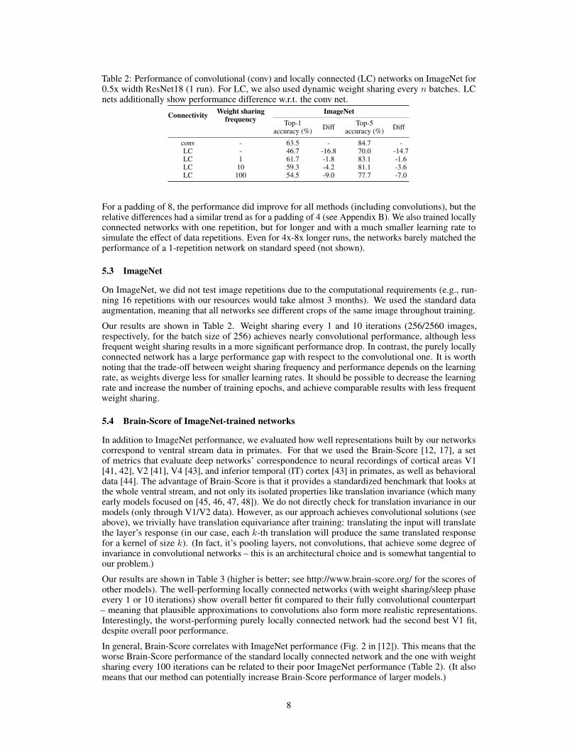
Table 2: Performance of convolutional (conv) and locally connected (LC) networks on ImageNet for0.5x width ResNet18 (1 run). For LC, we also used dynamic weight sharing every n batches. LCnets additionally show performance difference w.r.t. the conv net.

Connectivity Weight sharingfrequency

ImageNetTop-1

accuracy (%) Diff Top-5accuracy (%) Diff

conv - 63.5 - 84.7 -LC - 46.7 -16.8 70.0 -14.7LC 1 61.7 -1.8 83.1 -1.6LC 10 59.3 -4.2 81.1 -3.6LC 100 54.5 -9.0 77.7 -7.0

For a padding of 8, the performance did improve for all methods (including convolutions), but therelative differences had a similar trend as for a padding of 4 (see Appendix B). We also trained locallyconnected networks with one repetition, but for longer and with a much smaller learning rate tosimulate the effect of data repetitions. Even for 4x-8x longer runs, the networks barely matched theperformance of a 1-repetition network on standard speed (not shown).

5.3 ImageNet

On ImageNet, we did not test image repetitions due to the computational requirements (e.g., run-ning 16 repetitions with our resources would take almost 3 months). We used the standard dataaugmentation, meaning that all networks see different crops of the same image throughout training.

Our results are shown in Table 2. Weight sharing every 1 and 10 iterations (256/2560 images,respectively, for the batch size of 256) achieves nearly convolutional performance, although lessfrequent weight sharing results in a more significant performance drop. In contrast, the purely locallyconnected network has a large performance gap with respect to the convolutional one. It is worthnoting that the trade-off between weight sharing frequency and performance depends on the learningrate, as weights diverge less for smaller learning rates. It should be possible to decrease the learningrate and increase the number of training epochs, and achieve comparable results with less frequentweight sharing.

5.4 Brain-Score of ImageNet-trained networks

In addition to ImageNet performance, we evaluated how well representations built by our networkscorrespond to ventral stream data in primates. For that we used the Brain-Score [12, 17], a setof metrics that evaluate deep networks’ correspondence to neural recordings of cortical areas V1[41, 42], V2 [41], V4 [43], and inferior temporal (IT) cortex [43] in primates, as well as behavioraldata [44]. The advantage of Brain-Score is that it provides a standardized benchmark that looks atthe whole ventral stream, and not only its isolated properties like translation invariance (which manyearly models focused on [45, 46, 47, 48]). We do not directly check for translation invariance in ourmodels (only through V1/V2 data). However, as our approach achieves convolutional solutions (seeabove), we trivially have translation equivariance after training: translating the input will translatethe layer’s response (in our case, each k-th translation will produce the same translated responsefor a kernel of size k). (In fact, it’s pooling layers, not convolutions, that achieve some degree ofinvariance in convolutional networks – this is an architectural choice and is somewhat tangential toour problem.)

Our results are shown in Table 3 (higher is better; see http://www.brain-score.org/ for the scores ofother models). The well-performing locally connected networks (with weight sharing/sleep phaseevery 1 or 10 iterations) show overall better fit compared to their fully convolutional counterpart– meaning that plausible approximations to convolutions also form more realistic representations.Interestingly, the worst-performing purely locally connected network had the second best V1 fit,despite overall poor performance.

In general, Brain-Score correlates with ImageNet performance (Fig. 2 in [12]). This means that theworse Brain-Score performance of the standard locally connected network and the one with weightsharing every 100 iterations can be related to their poor ImageNet performance (Table 2). (It alsomeans that our method can potentially increase Brain-Score performance of larger models.)

8

http://www.brain-score.org/

Table 3: Brain-Score of ImageNet-trained convolutional (conv) and locally connected (LC) networkson ImageNet for 0.5x width ResNet18 (higher is better). For LC, we also used dynamic weightsharing every n batches. ∗The models were evaluated on Brain-Score benchmarks available duringsubmission. If new benchmarks are added and the models are re-evaluated on them, the final scoresmight change; the provided links contain the latest results.

Connectivity Weight sharingfrequency

Brain-Scoreaverage score V1 V2 V4 IT behavior link∗

conv - .357 .493 .313 .459 .370 .148 brain-score.org/model/876LC - .349 .542 .291 .448 .354 .108 brain-score.org/model/877LC 1 .396 .512 .339 .468 .406 .255 brain-score.org/model/880LC 10 .385 .508 .322 .478 .399 .216 brain-score.org/model/878LC 100 .351 .523 .293 .467 .370 .101 brain-score.org/model/879

6 Discussion

We presented two ways to circumvent the biological implausibility of weight sharing, a crucialcomponent of convolutional networks. The first was through data augmentation via multiple imagetranslations. The second was dynamic weight sharing via lateral connections, which allows neuronsto share weight information during a sleep-like phase; weight updates are then done using Hebbianplasticity. Data augmentation requires a large number of repetitions in the data, and, consequently,longer training times, and yields only small improvements in performance. However, only a smallnumber of repetitions can be naturally covered by saccades. Dynamic weight sharing needs a separatesleep phase, rather than more data, and yields large performance gains. In fact, it achieves nearconvolutional performance even on hard tasks, such as ImageNet classification, making it a muchmore likely candidate than data augmentation for the brain. In addition, well-performing locallyconnected networks trained with dynamic weight sharing achieve a better fit to the ventral streamdata (measured by the Brain-Score [12, 17]). The sleep phase can occur during actual sleep, when thenetwork (i.e., the visual system) stops receiving visual inputs, but maintains some internal activity.This is supported by plasticity studies during sleep (e.g. [49, 50]).

There are several limitations to our implementation of dynamic weight sharing. First, it relies onprecise lateral connectivity. This can be genetically encoded, or learned early on using correlations inthe input data (if layer l can generate repeated patters, layer l + 1 can modify its lateral connectivitybased on input correlations). Lateral connections do in fact exist in the visual stream, with neuronsthat have similar tuning curves showing strong lateral connections [51]. Second, the sleep phaseworks iteratively over layers. This can be implemented with neuromodulation that enables plasticityone layer at a time. Alternatively, weight sharing could work simultaneously in the whole networkdue to weight regularization (as it ensures that the final solution preserves the initial average weight),although this would require longer training due to additional noise in deep layers. Third, in ourscheme the lateral connections are used only for dynamic weight sharing, and not for training orinference. As our realistic model in Section 4.2 implements this connectivity via an inhibitory neuron,we can think of that neuron as being silent outside of the sleep phase. Finally, we trained networksusing backpropagation, which is not biologically plausible [18]. However, our weight sharing schemeis independent of the wake-phase training algorithm, and therefore can be applied along with anybiologically plausible update rule.

Our approach to dynamic weight sharing is not relevant only to convolutions. First, it is applicable tonon-convolutional networks, and in particular visual transformers [28, 29, 30, 31] (and more recentMLP-based architectures [32, 33, 34]). In such architectures, input images (and intermediate two-dimensional representations) are split into non-overlapping patches; each patch is then transformedwith the same fully connected layer – a computation that would require weight sharing in the brain.This can be done by connecting neurons across patches that have the same relative position, andapplying our weight dynamics (see Appendix A.4). Second, [23] faced a problem similar to weightsharing – weight transport (i.e., neurons not knowing their output weights) – when developing aplausible implementation of backprop. Their weight mirror algorithms used an idea similar to ours:the value of one weight was sent to another through correlations in activity.

Our study shows that both performance and the computation of convolutional networks can bereproduced in more realistic architectures. This supports convolutional networks as a model of the

9

http://www.brain-score.org/model/876





visual stream, and also justifies them as a “model organism” for studying learning in the visual stream(which is important partially due to their computational efficiency). While our study does not haveimmediate societal impacts (positive or negative), it further strengthens the role of artificial neuralnetworks as a model of the brain. Such models can guide medical applications such as brain machineinterfaces and neurological rehabilitation. However, that could also lead to the design of potentiallyharmful adversarial attacks on the brain.

Acknowledgments and Disclosure of Funding

The authors would like to thank Martin Schrimpf and Mike Ferguson for their help with the Brain-Score evaluation.

This work was supported by the Gatsby Charitable Foundation, the Wellcome Trust and DeepMind.

References

[1] Alex Krizhevsky, Ilya Sutskever, and Geoffrey E Hinton. Imagenet classification with deepconvolutional neural networks. Advances in neural information processing systems, 25:1097–1105, 2012.

[2] Karen Simonyan and Andrew Zisserman. Very deep convolutional networks for large-scaleimage recognition. arXiv preprint arXiv:1409.1556, 2014.

[3] Kaiming He, Xiangyu Zhang, Shaoqing Ren, and Jian Sun. Deep residual learning for imagerecognition. In Proceedings of the IEEE conference on computer vision and pattern recognition,pages 770–778, 2016.

[4] Ossama Abdel-Hamid, Abdel-rahman Mohamed, Hui Jiang, Li Deng, Gerald Penn, and DongYu. Convolutional neural networks for speech recognition. IEEE/ACM Transactions on audio,speech, and language processing, 22(10):1533–1545, 2014.

[5] Alexis Conneau, Holger Schwenk, Loïc Barrault, and Yann Lecun. Very deep convolutionalnetworks for text classification. arXiv preprint arXiv:1606.01781, 2016.

[6] Fazle Karim, Somshubra Majumdar, Houshang Darabi, and Shun Chen. Lstm fully convolutionalnetworks for time series classification. IEEE access, 6:1662–1669, 2017.

[7] Grace W. Lindsay. Convolutional Neural Networks as a Model of the Visual System: Past,Present, and Future. Journal of Cognitive Neuroscience, pages 1–15, 02 2020.

[8] David H Hubel and Torsten N Wiesel. Receptive fields, binocular interaction and functionalarchitecture in the cat’s visual cortex. The Journal of physiology, 160(1):106–154, 1962.

[9] Kunihiko Fukushima and Sei Miyake. Neocognitron: A self-organizing neural network modelfor a mechanism of visual pattern recognition. In Competition and cooperation in neural nets,pages 267–285. Springer, 1982.

[10] Daniel LK Yamins, Ha Hong, Charles F Cadieu, Ethan A Solomon, Darren Seibert, and James JDiCarlo. Performance-optimized hierarchical models predict neural responses in higher visualcortex. Proceedings of the national academy of sciences, 111(23):8619–8624, 2014.

[11] Seyed-Mahdi Khaligh-Razavi and Nikolaus Kriegeskorte. Deep supervised, but not un-supervised, models may explain it cortical representation. PLoS computational biology,10(11):e1003915, 2014.

[12] Martin Schrimpf, Jonas Kubilius, Ha Hong, Najib J. Majaj, Rishi Rajalingham, Elias B. Issa,Kohitij Kar, Pouya Bashivan, Jonathan Prescott-Roy, Franziska Geiger, Kailyn Schmidt, DanielL. K. Yamins, and James J. DiCarlo. Brain-score: Which artificial neural network for objectrecognition is most brain-like? bioRxiv preprint, 2018.

[13] Santiago A Cadena, George H Denfield, Edgar Y Walker, Leon A Gatys, Andreas S Tolias,Matthias Bethge, and Alexander S Ecker. Deep convolutional models improve predictions ofmacaque v1 responses to natural images. PLoS computational biology, 15(4):e1006897, 2019.

[14] Stephen Grossberg. Competitive learning: From interactive activation to adaptive resonance.Cognitive science, 11(1):23–63, 1987.

10

[15] Sergey Bartunov, Adam Santoro, Blake Richards, Luke Marris, Geoffrey E Hinton, and TimothyLillicrap. Assessing the scalability of biologically-motivated deep learning algorithms andarchitectures. In Advances in Neural Information Processing Systems, pages 9368–9378, 2018.

[16] Stéphane d’Ascoli, Levent Sagun, Joan Bruna, and Giulio Biroli. Finding the needle in thehaystack with convolutions: on the benefits of architectural bias. arXiv preprint arXiv:1906.06766,2019.

[17] Martin Schrimpf, Jonas Kubilius, Michael J Lee, N Apurva Ratan Murty, Robert Ajemian, andJames J DiCarlo. Integrative benchmarking to advance neurally mechanistic models of humanintelligence. Neuron, 2020.

[18] Blake A Richards, Timothy P Lillicrap, Philippe Beaudoin, Yoshua Bengio, Rafal Bogacz,Amelia Christensen, Claudia Clopath, Rui Ponte Costa, Archy de Berker, Surya Ganguli, et al. Adeep learning framework for neuroscience. Nature neuroscience, 22(11):1761–1770, 2019.

[19] Arild Nøkland. Direct feedback alignment provides learning in deep neural networks. InAdvances in neural information processing systems, pages 1037–1045, 2016.

[20] Theodore H Moskovitz, Ashok Litwin-Kumar, and LF Abbott. Feedback alignment in deepconvolutional networks. arXiv preprint arXiv:1812.06488, 2018.

[21] Hesham Mostafa, Vishwajith Ramesh, and Gert Cauwenberghs. Deep supervised learning usinglocal errors. Frontiers in neuroscience, 12:608, 2018.

[22] Arild Nøkland and Lars Hiller Eidnes. Training neural networks with local error signals. arXivpreprint arXiv:1901.06656, 2019.

[23] Mohamed Akrout, Collin Wilson, Peter Humphreys, Timothy Lillicrap, and Douglas B Tweed.Deep learning without weight transport. In Advances in Neural Information Processing Systems,pages 974–982, 2019.

[24] Axel Laborieux, Maxence Ernoult, Benjamin Scellier, Yoshua Bengio, Julie Grollier, andDamien Querlioz. Scaling equilibrium propagation to deep convnets by drastically reducing itsgradient estimator bias. arXiv preprint arXiv:2006.03824, 2020.

[25] Roman Pogodin and Peter E Latham. Kernelized information bottleneck leads to biologicallyplausible 3-factor hebbian learning in deep networks. arXiv preprint arXiv:2006.07123, 2020.

[26] Behnam Neyshabur. Towards learning convolutions from scratch. arXiv preprintarXiv:2007.13657, 2020.

[27] Gamaleldin Elsayed, Prajit Ramachandran, Jonathon Shlens, and Simon Kornblith. Revis-iting spatial invariance with low-rank local connectivity. In Hal Daumé III and Aarti Singh,editors, Proceedings of the 37th International Conference on Machine Learning, volume 119 ofProceedings of Machine Learning Research, pages 2868–2879. PMLR, 13–18 Jul 2020.

[28] Alexey Dosovitskiy, Lucas Beyer, Alexander Kolesnikov, Dirk Weissenborn, Xiaohua Zhai,Thomas Unterthiner, Mostafa Dehghani, Matthias Minderer, Georg Heigold, Sylvain Gelly, et al.An image is worth 16x16 words: Transformers for image recognition at scale. arXiv preprintarXiv:2010.11929, 2020.

[29] Nicolas Carion, Francisco Massa, Gabriel Synnaeve, Nicolas Usunier, Alexander Kirillov, andSergey Zagoruyko. End-to-end object detection with transformers. In European Conference onComputer Vision, pages 213–229. Springer, 2020.

[30] Hugo Touvron, Matthieu Cord, Matthijs Douze, Francisco Massa, Alexandre Sablayrolles, andHervé Jégou. Training data-efficient image transformers & distillation through attention. arXivpreprint arXiv:2012.12877, 2020.

[31] Xizhou Zhu, Weijie Su, Lewei Lu, Bin Li, Xiaogang Wang, and Jifeng Dai. Deformable detr:Deformable transformers for end-to-end object detection. arXiv preprint arXiv:2010.04159,2020.

[32] Ilya Tolstikhin, Neil Houlsby, Alexander Kolesnikov, Lucas Beyer, Xiaohua Zhai, ThomasUnterthiner, Jessica Yung, Daniel Keysers, Jakob Uszkoreit, Mario Lucic, and Alexey Dosovitskiy.Mlp-mixer: An all-mlp architecture for vision, 2021.

[33] Hugo Touvron, Piotr Bojanowski, Mathilde Caron, Matthieu Cord, Alaaeldin El-Nouby,Edouard Grave, Armand Joulin, Gabriel Synnaeve, Jakob Verbeek, and Hervé Jégou. Resmlp:Feedforward networks for image classification with data-efficient training. arXiv preprintarXiv:2105.03404, 2021.

11

[34] Hanxiao Liu, Zihang Dai, David R So, and Quoc V Le. Pay attention to mlps. arXiv preprintarXiv:2105.08050, 2021.

[35] Alex Krizhevsky, Geoffrey Hinton, et al. Learning multiple layers of features from tiny images.2009.

[36] Ya Le and Xuan Yang. Tiny imagenet visual recognition challenge. CS 231N, 7:7, 2015.[37] Jia Deng, Wei Dong, Richard Socher, Li-Jia Li, Kai Li, and Li Fei-Fei. Imagenet: A large-

scale hierarchical image database. In 2009 IEEE conference on computer vision and patternrecognition, pages 248–255. Ieee, 2009.

[38] Ilya Loshchilov and Frank Hutter. Decoupled weight decay regularization. arXiv preprintarXiv:1711.05101, 2017.

[39] Adam Paszke, Sam Gross, Francisco Massa, Adam Lerer, James Bradbury, Gregory Chanan,Trevor Killeen, Zeming Lin, Natalia Gimelshein, Luca Antiga, Alban Desmaison, AndreasKopf, Edward Yang, Zachary DeVito, Martin Raison, Alykhan Tejani, Sasank Chilamkurthy,Benoit Steiner, Lu Fang, Junjie Bai, and Soumith Chintala. Pytorch: An imperative style, high-performance deep learning library. In H. Wallach, H. Larochelle, A. Beygelzimer, F. d'Alché-Buc,E. Fox, and R. Garnett, editors, Advances in Neural Information Processing Systems 32, pages8024–8035. Curran Associates, Inc., 2019.

[40] Jordan Ott, Erik J. Linstead, Nicholas LaHaye, and Pierre Baldi. Learning in the machine: Toshare or not to share? Neural networks : the official journal of the International Neural NetworkSociety, 126:235–249, 2020.

[41] Jeremy Freeman, Corey M. Ziemba, David J. Heeger, Eero P. Simoncelli, and J. AnthonyMovshon. A functional and perceptual signature of the second visual area in primates. NatureNeuroscience, 16(7):974–981, Jul 2013.

[42] Tiago Marques, Martin Schrimpf, and James J DiCarlo. Multi-scale hierarchical neural networkmodels that bridge from single neurons in the primate primary visual cortex to object recognitionbehavior. bioRxiv, 2021.

[43] Najib J. Majaj, Ha Hong, Ethan A. Solomon, and James J. DiCarlo. Simple learned weightedsums of inferior temporal neuronal firing rates accurately predict human core object recognitionperformance. Journal of Neuroscience, 35(39):13402–13418, 2015.

[44] Rishi Rajalingham, Elias B. Issa, Pouya Bashivan, Kohitij Kar, Kailyn Schmidt, and James J.DiCarlo. Large-scale, high-resolution comparison of the core visual object recognition behaviorof humans, monkeys, and state-of-the-art deep artificial neural networks. bioRxiv, 2018.

[45] Maximilian Riesenhuber and Tomaso A. Poggio. Hierarchical models of object recognition incortex. Nature Neuroscience, 2:1019–1025, 1999.

[46] Peter Földiák. Learning invariance from transformation sequences. Neural computation,3(2):194–200, 1991.

[47] Guy Wallis, Edmund Rolls, and Peter Foldiak. Learning invariant responses to the naturaltransformations of objects. In Proceedings of 1993 International Conference on Neural Networks(IJCNN-93-Nagoya, Japan), volume 2, pages 1087–1090. IEEE, 1993.

[48] Laurenz Wiskott and Terrence J Sejnowski. Slow feature analysis: Unsupervised learning ofinvariances. Neural computation, 14(4):715–770, 2002.

[49] Sushil K Jha, Brian E. Jones, Tammi Coleman, Nick Steinmetz, Chi-Tat Law, Gerald D. Griffin,Joshua D. Hawk, Nooreen Dabbish, Valery A. Kalatsky, and Marcos G. Frank. Sleep-dependentplasticity requires cortical activity. The Journal of Neuroscience, 25:9266 – 9274, 2005.

[50] Carlos Puentes-Mestril and Sara J Aton. Linking network activity to synaptic plasticity duringsleep: hypotheses and recent data. Frontiers in neural circuits, 11:61, 2017.

[51] William H. Bosking, Ying Zhang, Brett Schofield, and David Fitzpatrick. Orientation selectivityand the arrangement of horizontal connections in tree shrew striate cortex. J. Neurosci., 15, 1997.

[52] Robert Mansel Gower, Nicolas Loizou, Xun Qian, Alibek Sailanbayev, Egor Shulgin, and PeterRichtárik. Sgd: General analysis and improved rates. In International Conference on MachineLearning, pages 5200–5209. PMLR, 2019.

[53] Kaiming He, Xiangyu Zhang, Shaoqing Ren, and Jian Sun. Delving deep into rectifiers:Surpassing human-level performance on imagenet classification. In Proceedings of the IEEEinternational conference on computer vision, pages 1026–1034, 2015.

12

Checklist

1. For all authors...(a) Do the main claims made in the abstract and introduction accurately reflect the paper’s

contributions and scope? [Yes](b) Did you describe the limitations of your work? [Yes] See Section 6.(c) Did you discuss any potential negative societal impacts of your work? [Yes] See

Section 6.(d) Have you read the ethics review guidelines and ensured that your paper conforms to

them? [Yes]2. If you are including theoretical results...

(a) Did you state the full set of assumptions of all theoretical results? [Yes] See thesupplementary material.

(b) Did you include complete proofs of all theoretical results? [Yes] See the supplementarymaterial.

3. If you ran experiments...(a) Did you include the code, data, and instructions needed to reproduce the main ex-

perimental results (either in the supplemental material or as a URL)? [Yes] Seehttps://github.com/romanpogodin/towards-bio-plausible-conv and the supplementarymaterial.

(b) Did you specify all the training details (e.g., data splits, hyperparameters, how theywere chosen)? [Yes] See the supplementary material.

(c) Did you report error bars (e.g., with respect to the random seed after running ex-periments multiple times)? [Yes] See the supplementary material for small-scaleexperiments. [No] The large-scale experiments were run 1 time due to resource con-straints.

(d) Did you include the total amount of compute and the type of resources used (e.g., typeof GPUs, internal cluster, or cloud provider)? [Yes] See Section 5.

4. If you are using existing assets (e.g., code, data, models) or curating/releasing new assets...(a) If your work uses existing assets, did you cite the creators? [Yes](b) Did you mention the license of the assets? [No] We used publicly available datasets

and open-source repositories.(c) Did you include any new assets either in the supplemental material or as a URL? [Yes]

Implementation: https://github.com/romanpogodin/towards-bio-plausible-conv(d) Did you discuss whether and how consent was obtained from people whose data you’re

using/curating? [No] We used publicly available datasets.(e) Did you discuss whether the data you are using/curating contains personally identifiable

information or offensive content? [No] We used publicly available datasets.5. If you used crowdsourcing or conducted research with human subjects...

(a) Did you include the full text of instructions given to participants and screenshots, ifapplicable? [N/A]

(b) Did you describe any potential participant risks, with links to Institutional ReviewBoard (IRB) approvals, if applicable? [N/A]

(c) Did you include the estimated hourly wage paid to participants and the total amountspent on participant compensation? [N/A]

13



Appendices

A Dynamic weight sharing

A.1 Noiseless case

Each neuron receives the same k-dimensional input x, and its response zi is given by

zi = w>i x =

k∑j=1

wijxj . (10)

To equalize the weights wi among all neurons, the network minimizes the following objective,

Lw. sh.(w1, . . . ,wN ) =1

4MN

M∑m=1

N∑i=1

N∑j=1

(zi − zj)2 +γ

2

N∑i=1

‖wi − winiti ‖2 (11)

=1

4MN

M∑m=1

N∑i=1

N∑j=1

(w>i xm − w>j xm

)2+γ

2

N∑i=1

‖wi − winiti ‖2 , (12)

where winiti is the weight at the start of dynamic weight sharing. This is a strongly convex function,

and therefore it has a unique minimum.

The SGD update for one xm is

∆wi ∝ −

zi − 1

N

N∑j=1

zj

xm − γ(wi −winit

i

). (13)

To find the fixed point of the dynamics, we first set the sum over the gradients to zero,

∑i

dLw. sh.(w1, . . . ,wN )

dwi=

1

M

∑i,m

zi − 1

N

N∑j=1

zj

xm + γ∑i

(wi −winit

i

)(14)

= γ∑i

(wi −winit

i

)= 0 . (15)

Therefore, at the fixed point the mean weight µ∗ =∑i w∗i /N is equal to µinit =

∑i winit

i /N , and

1

N

N∑i=1

zi =1

N

N∑i=1

w∗>i xm = (µinit)> xm . (16)

We can now find the individual weights,

dLw. sh.(w1, . . . ,wN )

dwi=

1

M

∑m

zi − 1

N

N∑j=1

zj

xm + γ(wi −winit

i

)(17)

=1

M

∑m

xmx>m(wi − µinit

)+ γ

(wi −winit

i

)= 0 . (18)

Denoting the covariance matrix C ≡ 1M

∑m xmx>m, we see that

w∗i = (C + γ I)−1(Cµinit + γwinit

i

)= (C + γ I)−1

(C

1

N

N∑i=1

winiti + γwinit

i

), (19)

where I is the identity matrix. From Eq. (19) it is clear that w∗i ≈ µinit for small γ and full rank C.For instance, for C = I,

w∗i =1

1 + γµinit +

γ

1 + γwiniti . (20)

14

0 0-2-4-6

-8-10-12

-2

-4

-6

-8

-10

BA

𝛾=1e-1𝛾=1e-2

𝛾=1e-3

𝛾=1e-1𝛾=1e-2

𝛾=1e-3

k=3 k=9 k=18

-log SNRw -log SNRw

iter 0 2k 4k 6k 8k0 2k 4k 6k 8k iter

Figure 5: Logarithm of inverse signal-to-noise ratio (mean weight squared over weight variance,see Eq. (6)) for weight sharing objectives in a layer with 100 neurons. A. Dynamics of Eq. (21) fordifferent kernel sizes k (meaning k2 inputs) and γ. B. Dynamics of weight update that uses Eq. (8b)for α = 10, different kernel sizes k and γ. In each iteration, the input is presented for 150 ms.

A.2 Biased noiseless case, and its correspondence to the realistic implementation

The realistic implementation of dynamic weight sharing with an inhibitory neuron (Section 4.2)introduces a bias in the update rule: Eq. (13) becomes

∆wi ∝ −

zi − α

N(1 + α)

N∑j=1

zj

xm − γ(wi −winit

i

)(21)

for inhibition strength α.

Following the same derivation as for the unbiased case, we can show that the weight dynamicsconverges to

∑i

dLw. sh.(w1, . . . ,wN )

dwi=

1

M

∑i,m

zi − α

1 + α

1

N

N∑j=1

zj

xm + γ∑i

(wi −winit

i

)(22)

=1

1 + αC∑i

wi + γ∑i

(wi −winit

i

)= 0 . (23)

Therefore µ∗ = γ(

11+αC + γI

)−1µinit, and

w∗i = (C + γ I)−1(

γα

1 + αC(

1

1 + αC + γI

)−1µinit + γwinit

i

). (24)

For C = I, this becomes

w∗i =γ

1 + γ

(α

1 + γ(1 + α)µinit + winit

i

). (25)

As a result, the final weights are approximately the same among neurons, but have a small norm dueto the γ scaling.

The dynamics in Eq. (21) correctly captures the bias influence in Eq. (8b), producing similar SNRplots; compare Fig. 5A (Eq. (21) dynamics) to Fig. 5B (Eq. (8b) dynamics). The curves are slightlydifferent due to different learning rates, but both follow the same trend of first finding a very goodsolution, and then slowly incorporating the bias term (leading to smaller SNR).

15

A.3 Noisy case

Realistically, all neurons can’t see the same xm. However, due to the properties of our loss, we canwork even with noisy updates. To see this, we write the objective function as

Lw. sh.(w1, . . . ,wN ) =1

M

M∑m=1

f(W,Xm) (26)

where matrices W and X satisfy (W)i = wi and (Xm)i = xm, and

f(W,Xm) =1

4N

N∑i=1

N∑j=1

(w>i xm − w>i xm

)2+γ

2

N∑i=1

‖wi − winiti ‖2 . (27)

We’ll update the weights with SGD according to

∆Wk+1 = −ηkd

dWf(W,Xm(k) + Ek)

∣∣∣∣Wk

, (28)

where (Ek)i = εi is zero-mean input noise and m(k) is chosen uniformly.

Let’s also bound the input mean and noise as

EE

∥∥xm(k) + εi∥∥2 ≤ √cxε, EE

∥∥xm(k) + εi∥∥4 ≤ cxε . (29)

With this setup, we can show that SGD with noise can quickly converge to the correct solution, apartfrom a constant noise-induced bias. Our analysis is standard and follows [52], but had to be adaptedfor our objective and noise model.Theorem 1. For zero-mean isotropic noise E with variance σ2, uniform SGD sampling m(k) andinputs xm that satisfy Eq. (29), choosing ηk = O(1/k) leads to

E ‖Wk+1 −W∗‖2F = O

(∥∥Winit −W∗∥∥F

k + 1

)+O

(σ2‖W∗‖2F

), (30)

where (W∗)i is given by Eq. (19).

Proof. Using the SGD update,

‖Wk+1 −W∗‖2F =

∥∥∥∥Wk − ηkd

dWf(W,Xm(k) + Ek)

∣∣∣∣Wk

−W∗∥∥∥∥2F

(31)

=∥∥Wk −W∗∥∥2

F− 2ηk

⟨Wk −W∗,

d

dWf(W,Xm(k) + Ek)

∣∣∣∣Wk

⟩(32)

+ η2k

∥∥∥∥ d

dWf(W,Xm(k) + Ek)

∣∣∣∣Wk

∥∥∥∥2F

. (33)

We need to bound the second and the third terms in the equation above.

Second term. As f is γ-strongly convex in W,

−⟨Wk −W∗,

d

dWf(W,Xm(k) + Ek)

∣∣∣∣Wk

⟩(34)

≤ f(W∗,Xm(k) + Ek)− f(Wk,Xm(k) + Ek)− γ

2‖Wk −W∗‖2F . (35)

As f is convex in X,

f(W∗,Xm(k) + Ek)− f(Wk,Xm(k) + Ek) ≤ f(W∗,Xm(k))− f(Wk,Xm(k)) (36)

+

⟨d

dXf(W∗,X)

∣∣∣∣Xm(k)+Ek

− d

dXf(Wk,X)

∣∣∣∣Xm(k)

, Ek

⟩. (37)

16

We only need to clarify one term here,(d

dXf(W∗,X)


)i

=

(d

dXf(W∗,X)

∣∣∣∣Xm(k)

)i

+

w∗>i εi −1

N

∑j

w∗>j εj

w∗i .

(38)

Now we can take the expectation over m(k) and E. As m(k) is uniform, and W∗ minimizes theglobal function,

Em(k)

(f(W∗,Xm(k))− f(Wk,Xm(k))

)= Lw. sh.(w∗1, . . . ,w

∗N )− Lw. sh.(wk1 , . . . ,w

kN ) ≤ 0 .

(39)As Ek is zero-mean and isotropic with variance σ2,

Em(k),Ek

⟨d

dXf(W∗,X)


− d

dXf(Wk,X)

∣∣∣∣Xm(k)

, Ek

⟩(40)

= EEk

∑i

w∗>i εi −1

N

∑j

w∗>j εj

w∗>i εi =

(1− 1

N

)EEk

∑i

(w∗>i εi

)2(41)

=

(1− 1

N

)EEk

∑i

Tr(w∗iw

∗>i εiε

>i

)≤ σ2‖W∗‖2F . (42)

So the whole second term becomes

− 2ηkEm(k),E

⟨Wk −W∗,

d

dWf(W,Xm(k) + Ek)

∣∣∣∣Wk

⟩(43)

≤ −γηkEm(k),Ek‖Wk −W∗‖2F + ηkσ2‖W∗‖2F . (44)

Third term. First, observe thatd

dwif(W,X) = xix>i wi − xi

1

N

∑j

x>j wj + γwi − γwiniti (45)

=

(1− 1

N

)Aiwi −BiW + γwi − γwinit

i , (46)

where Ai = xix>i and (Bi)j = I[i 6= j]xix>j /N .

Therefore, using ‖a+b‖2 ≤ 2‖a‖2+2‖b‖2 twice, properties of the matrix 2-norm, and (1−1/N) ≤ 1,∥∥∥∥ d

dwif(W,X)

∥∥∥∥2 ≤ 4 ‖Ai‖22 ‖wi‖2

+ 4 ‖Bi‖22 ‖W‖2

+ 4γ2 ‖wi‖2 + 4γ2∥∥winit

i

∥∥2 . (47)

In our particular case, bounding the 2 norm with the Frobenius norm gives

Em(k),E ‖Ai‖22 ≤ Em(k),E

∥∥(xm(k) + εi)(xm(k) + εi)>∥∥2

F(48)

= Em(k),E

∥∥xm(k) + εi∥∥4 ≤ cxε . (49)

Similarly,

Em(k),E ‖Bi‖22 ≤ Em(k),E ‖Bi‖2F ≤1

N2Em(k),E

∑j 6=i

∥∥xm(k) + εi∥∥2 ∥∥xm(k) + εj

∥∥2 ≤ cxεN

.

(50)

Therefore, we can bound the full gradient by the sum of individual bounds (as it’s the Frobeniusnorm) and using ‖a+ b‖2 ≤ 2‖a‖2 + 2‖b‖2 again,

Em(k),E

∥∥∥∥ d

dWf(W,Xm(k)+Ek)

∣∣∣∣Wk

∥∥∥∥2F

≤ 4(2cxε + γ2)∥∥Wk

∥∥2F

+ 4γ2∥∥Winit

∥∥2F

(51)

≤ 8(2cxε + γ2)∥∥Wk −W∗∥∥2

F+ 8(2cxε + γ2) ‖W∗‖2F + 4γ2

∥∥Winit∥∥2F. (52)

17

Combining all of this, and taking the expectation over all steps before k + 1, gives us

E ‖Wk+1 −W∗‖2F ≤(1− γηk + η2k8(2cxε + γ2)

)E∥∥Wk −W∗∥∥2

F(53)

+ ηkσ2‖W∗‖2F + η2k

(8(2cxε + γ2) ‖W∗‖2F + 4γ2

∥∥Winit∥∥2F

). (54)

If we choose ηk such that ηk ·(

8(2cxε + γ2) ‖W∗‖2F + 4γ2∥∥Winit

∥∥2F

)≤ σ2, we can simplify the

result,

E ‖Wk+1 −W∗‖2F ≤(1− γηk + η2k8(2cxε + γ2)

)E∥∥Wk −W∗∥∥2

F+ 2ηkσ

2‖W∗‖2F (55)

≤

(k∏s=0

(1− γηs + η2s8(2cxε + γ2)

))E∥∥Winit −W∗∥∥2

F(56)

+ 2σ2k∑t=0

ηt

(t∏

s=1

(1− γηs + η2s8(2cxε + γ2)

))‖W∗‖2F . (57)

If we choose ηk = O(1/k), the first term will decrease as 1/k. The second one will stay constantwith time, and proportional to σ2.

A.4 Applicability to vision transformers

In vision transformers (e.g. [28]), an input image is reshaped into a matrix Z ∈ RN×D for Nnon-overlapping patches of the input, each of size D. As the first step, Z is multiplied by a matrixU ∈ RD×3D as Z′ = ZU. Therefore, an output neuron z′ij =

∑k zikukj looks at zi with the same

weights as z′i′j =∑k zi′kukj uses for zi′ for any i′.

To share weights with dynamic weight sharing, for each k we need to connect all zik across i (inputlayer), and for each j – all z′ij across i (output layer). After that, weight sharing will proceed justlike for locally connected networks: activate an input grid j1 (one of D possible ones) to create arepeating input patter, then activate a grid j2 and so on.

A.5 Details for convergence plots

Both plots in Fig. 4 show mean negative log SNR over 10 runs, 100 output neurons each. Initialweights were drawn from N (1, 1). At every iteration, the new input x was drawn from N (1, 1)independently for each component. Learning was performed via SGD with momentum of 0.95.The minimum SNR value was computed from Eq. (5). For our data, the SNR expression inEq. (6) has

(1N

∑i(wi)j

)2 ≈ 1 and 1N

∑i

((wi)j − 1

N

∑i′(wi′)j

)2 ≈ γ2/(1 + γ)2, therefore− log SNRmin = 2 log(γ/(1 + γ)).

For Fig. 4A, we performed 2000 iterations (with a new x each time). Learning rate at iteration k wasηk = 0.5/(1000 + k). For Fig. 5A, we did the same simulation but for 104 iterations.

For Fig. 4B, network dynamics (Eq. (8b)) was simulated with τ = 30 ms, b = 1 using Euler methodwith steps size of 1 ms. We performed 104 iterations (150 ms per iteration, with a new x eachiteration). Learning rate at iteration k was ηk = 0.0003/

√1 + k/2 · I[k ≥ 50].

The code for both runs is provided in the supplementary material.

B Experimental details

Both convolutional and LC layers did not have the bias term, and were initialized according to KaimingNormal initialization [53] with ReLU gain, meaning each weight was drawn from N (0, 2/(coutk

2))for kernel size k and cout output channels.

All runs were done with automatic mixed precision, meaning that inputs to each layer (but not theweights) were stored as float16, and not float32. This greatly improved performance and memoryrequirements of the networks.

18

As an aside, the weight dynamics of sleep/training phases indeed followed Fig. 3A. Fig. 6 shows− log SNRw (defined in Eq. (6)) for weight sharing every 10 iterations on CIFAR10. For smalllearning rates, the weights do not diverge too much in-between sleep phases.

0 20 40 60 80

403530252015105

0 20 40 60 80

40

30

20

10

0

0 20 40 60 80

40

30

20

10

0A -log SNRw

iter

B -log SNRw

iter

C -log SNRw

iter

Figure 6: Logarithm of inverse signal-to-noise ratio (mean weight squared over weight variance, seeEq. (6)) for weight sharing every 10 iterations for CIFAR10. A. Learning rate = 5e-4. B. Learningrate = 5e-3. C. Learning rate = 5e-2.

B.1 CIFAR10/100, TinyImageNet

Mean performance over 5 runs is summarized in Table 4 (padding of 0), Table 5 (padding of 4), andTable 6 (padding of 8). Maximum minus minimum accuracy is summarized in Table 7, Table 8, andTable 9. Hyperparameters for AdamW (learning rate and weight decay) are provided in Table 10,Table 11, and Table 12.

Hyperparameters were optimized on a train/validation split (see Section 5) over the following grids.CIFAR10/100. Learning rate: [1e-1, 5e-2, 1e-2, 5e-3] (conv), [1e-3, 5e-4, 1e-4, 5e-5] (LC); weightdecay [1e-2, 1e-4] (both). TinyImageNet. Learning rate: [5e-3, 1e-3, 5e-4] (conv), [1e-3, 5e-4](LC); weight decay [1e-2, 1e-4] (both). The learning rate range for TinyImageNet was smaller aspreliminary experiments showed poor performance for slow learning rates.

For all runs, the batch size was 512. For all final runs, learning rate was divided by 4 at 100 and thenat 150 epochs (out of 200). Grid search for CIFAR10/100 was done for the same 200 epochs setup.For TinyImageNet, grid search was performed over 50 epochs with learning rate decreases at 25 and37 epochs (i.e., the same schedule but compressed) due to the larger computational cost of full runs.

B.2 ImageNet

In addition to the main results, we also tested the variant of the locally connected network with aconvolutional first layer (Table 13). It improved performance for all configurations: from about 2%for weight sharing every 1-10 iterations, to about 5% for 100 iterations and for no weight sharing.This is not surprising, as the first layer has the largest resolution (224 by 224; initially, we performedthese experiment due to memory constraints). Our result suggests that adding a “good” pre-processinglayer (e.g. the retina) can also improve performance of locally connected networks.

Final hyperparameters. Learning rate: 1e-3 (conv, LC with w.sh. (1)), 5e-4 (all other LC; all LCwith 1st layer conv), weight decay: 1e-2 (all). Hyperparameters were optimized on a train/validationsplit (see Section 5) over the following grids. Conv: learning rate [1e-3, 5e-4], weight decay [1e-2,1e-4, 1e-6]. LC: learning rate [1e-3, 5e-4, 1e-4, 5e-5], weight decay [1e-2]. LC (1st layer conv):learning rate [1e-3, 5e-4], weight decay [1e-2, 1e-4, 1e-6]. For LC, we only tried the large weightdecay based on earlier experiment (LC (1st layer conv)). For LC (1st layer conv), we only tunedhyperparameters for LC and LC with weight sharing in each iteration, as they found the same values(weight sharing every 10/100 iterations interpolates between LC and LC with weight sharing in eachiteration, and therefore is expected to behave similarly to both). In addition, for LC (1st layer conv)we only tested learning rate of 5e-4 for weight decay of 1e-2 as higher learning rates performedsignificantly worse for other runs (and in preliminary experiments).

For all runs, the batch size was 256. For all final runs, learning rate was divided by 4 at 100 and thenat 150 epochs (out of 200). Grid search was performed over 20 epochs with learning rate decreases at

19

Table 4: Performance of convolutional (conv) and locally connected (LC) networks for padding of 0in the input images (mean accuracy over 5 runs). For LC, two regularization strategies were applied:repeating the same image n times with different translations (n reps) or using dynamic weight sharingevery n batches (ws (n)). LC nets additionally show performance difference w.r.t. conv nets.




accuracy (%) Diff

- conv 84.1 - 49.5 - 78.2 - 26.0 - 51.2 -LC 67.2 -16.8 34.9 -14.6 62.2 -16.0 12.0 -14.1 30.4 -20.7

Weight SharingLC - ws(1) 74.8 -9.3 41.8 -7.7 70.1 -8.1 24.9 -1.2 49.1 -2.1LC - ws(10) 75.9 -8.1 44.4 -5.1 72.0 -6.2 28.1 2.0 52.5 1.3

LC - ws(100) 75.4 -8.6 43.4 -6.1 71.9 -6.3 27.4 1.3 51.9 0.8

Table 5: Mean performance over 5 runs. Same as Table 4, but for padding of 4.Regularizer Connectivity CIFAR10 CIFAR100 TinyImageNet

Top-1accuracy (%) Diff Top-1



- conv 88.3 - 59.2 - 84.9 - 38.6 - 65.1 -LC 80.9 -7.4 49.8 -9.4 75.5 -9.4 29.6 -9.0 52.7 -12.4


LC - 16 reps 85.0 -3.3 55.9 -3.3 78.8 -6.1 34.0 -4.6 56.2 -8.8

Weight SharingLC - ws(1) 87.4 -0.8 58.7 -0.5 83.4 -1.6 41.6 3.0 66.1 1.1

LC - ws(10) 85.1 -3.2 55.7 -3.6 80.9 -4.0 37.4 -1.2 61.8 -3.2LC - ws(100) 82.0 -6.3 52.8 -6.4 80.1 -4.8 37.1 -1.5 62.8 -2.3

10 and 15 epochs (i.e., the same schedule but compressed) due to the large computational cost of fullruns.

Table 6: Mean performance over 5 runs. Same as Table 4, but for padding of 8.Regularizer Connectivity CIFAR10 CIFAR100 TinyImageNet

Top-1accuracy (%) Diff Top-1



- conv 88.7 - 59.6 - 85.4 - 42.6 - 68.7 -LC 80.7 -8.0 47.7 -11.8 74.8 -10.6 31.9 -10.7 55.4 -13.3


LC - 16 reps 85.0 -3.8 55.6 -4.0 78.4 -7.0 37.9 -4.7 60.3 -8.4

Weight SharingLC - ws(1) 87.8 -0.9 59.2 -0.4 84.0 -1.4 43.6 1.0 67.9 -0.9

LC - ws(10) 84.3 -4.5 53.7 -5.8 80.4 -5.0 39.6 -2.9 64.5 -4.3LC - ws(100) 79.5 -9.3 50.0 -9.6 78.6 -6.8 39.2 -3.4 64.8 -3.9

20

Table 7: Max minus min performance over 5 runs; padding of 0.


accuracy (%)Top-1

accuracy (%)Top-5

accuracy (%)Top-1

accuracy (%)Top-5

accuracy (%)

- conv 0.5 1.0 1.7 1.0 0.4LC 0.4 1.6 1.5 1.0 1.7

Weight SharingLC - ws(1) 0.5 1.3 1.3 1.2 2.0LC - ws(10) 0.8 1.0 0.7 1.8 2.1

LC - ws(100) 0.9 0.7 0.9 1.0 1.3



accuracy (%)Top-1

accuracy (%)Top-5

accuracy (%)Top-1

accuracy (%)Top-5

accuracy (%)

- conv 0.7 1.5 0.2 1.2 1.1LC 0.8 1.1 0.4 0.7 0.8

Data TranslationLC - 4 reps 0.8 1.3 0.8 0.5 0.8LC - 8 reps 0.3 1.4 1.3 0.7 1.2

LC - 16 reps 0.7 0.7 0.6 0.9 0.5

Weight SharingLC - ws(1) 0.5 1.1 0.9 0.9 0.6

LC - ws(10) 0.6 1.1 0.3 0.6 1.2LC - ws(100) 0.7 1.0 0.6 0.2 0.9



accuracy (%)Top-1

accuracy (%)Top-5

accuracy (%)Top-1

accuracy (%)Top-5

accuracy (%)

- conv 0.9 1.5 1.2 1.7 1.0LC 0.5 0.6 0.5 0.5 0.9

Data TranslationLC - 4 reps 0.4 0.9 0.3 0.6 0.8LC - 8 reps 0.6 0.9 0.5 0.5 0.6

LC - 16 reps 0.9 0.9 0.6 0.5 1.1

Weight SharingLC - ws(1) 0.4 1.2 1.5 0.7 0.7

LC - ws(10) 0.2 1.4 0.9 1.4 1.2LC - ws(100) 0.4 0.5 0.7 0.7 0.9

Table 10: Hyperparameters for padding of 0.

Regularizer Connectivity CIFAR10 CIFAR100 TinyImageNetLearning

rateWeightdecay

Learningrate

Weightdecay

Learningrate

Weightdecay

- conv 0.01 0.01 0.01 0.01 0.005 0.01LC 0.001 0.01 0.001 0.01 0.001 0.0001

Weight SharingLC - ws(1) 0.001 0.01 0.001 0.01 0.001 0.0001LC - ws(10) 0.0005 0.01 0.0005 0.0001 0.0005 0.01

LC - ws(100) 0.0001 0.01 0.0001 0.01 0.001 0.0001

21



rateWeightdecay

Learningrate

Weightdecay

Learningrate

Weightdecay

- conv 0.01 0.0001 0.01 0.01 0.005 0.0001LC 0.001 0.0001 0.0005 0.01 0.0005 0.0001

Data TranslationLC - 4 reps 0.001 0.01 0.001 0.01 0.0005 0.01LC - 8 reps 0.0005 0.01 0.0005 0.0001 0.0005 0.01

LC - 16 reps 0.0005 0.01 0.0005 0.01 0.0005 0.01

Weight SharingLC - ws(1) 0.001 0.01 0.001 0.0001 0.001 0.01

LC - ws(10) 0.0005 0.01 0.0005 0.01 0.001 0.0001LC - ws(100) 0.0005 0.01 0.0005 0.01 0.001 0.01



rateWeightdecay

Learningrate

Weightdecay

Learningrate

Weightdecay

- conv 0.01 0.01 0.01 0.01 0.005 0.01LC 0.001 0.01 0.0005 0.0001 0.001 0.01

Data TranslationLC - 4 reps 0.0005 0.01 0.001 0.0001 0.0005 0.01LC - 8 reps 0.001 0.01 0.0005 0.0001 0.0005 0.0001

LC - 16 reps 0.0005 0.0001 0.0005 0.01 0.0005 0.01

Weight SharingLC - ws(1) 0.001 0.0001 0.001 0.01 0.001 0.01

LC - ws(10) 0.0005 0.01 0.0005 0.0001 0.001 0.0001LC - ws(100) 0.0005 0.01 0.0005 0.0001 0.001 0.0001

Table 13: Performance of convolutional (conv), locally connected (LC) and locally connected withconvolutional first layer (LC + 1st layer conv) networks on ImageNet (1 run). For LC, we also useddynamic weight sharing every n batches. LC nets additionally show performance difference w.r.t. theconv net.

Model Connectivity Weight sharingfrequency

ImageNetTop-1


0.5x ResNet18

conv - 63.5 - 84.7 -LC - 46.7 -16.8 70.0 -14.7LC 1 61.7 -1.8 83.1 -1.6LC 10 59.3 -4.2 81.1 -3.6LC 100 54.5 -9.0 77.7 -7.0

0.5x ResNet18(1st layer conv)

LC - 52.2 -11.3 75.1 -9.6LC 1 63.6 0.1 84.5 -0.2LC 10 61.6 -1.9 83.1 -1.6LC 100 59.1 -4.4 81.1 -3.6

22

Towards Biologically Plausible Convolutional Networks

Documents

Transcript of Towards Biologically Plausible Convolutional Networks