Toward Simple Criteria to Establish Capacity Scaling Laws forWireless Networks

Canming Jiang† Yi Shi† Y. Thomas Hou†∗ Wenjing Lou†

Sastry Kompella‡ Scott F. Midkiff†

† Virginia Polytechnic Institute and State University, USA‡ US Naval Research Laboratory, Washington, DC, USA

Abstract

Capacity scaling laws offer fundamental understanding on the trend of user throughput behavior when the

network size increases. Since the seminal work of Gupta and Kumar, there have been active research efforts

in developing capacity scaling laws for ad hoc networks under various advanced physical layer technologies.

These efforts led to different custom-designed solutions,most of which were intellectually challenging and lacked

universal properties that can be extended to address scaling laws of ad hoc networks with other physical layer

technologies. In this paper, we present a set of simple yet powerful general criteria that one can apply to quickly

determine the capacity scaling laws for various physical layer technologies under the protocol model. We prove

the correctness of our proposed criteria and demonstrate their usage through a number of case studies, such as ad

hoc networks with directional antenna, MIMO, multi-channel multi-radio, cognitive radio, and multiple packet

reception. These simple criteria will serve as powerful tools to networking researchers to obtain throughput

scaling laws of ad hoc networks under different physical layer technologies, particularly those to be developed in

the future.

Keywords

Asymptotic capacity, scaling law, physical layer technology

1 Introduction

Capacity scaling laws refer to how a user’s throughput scales as the network size increases to infinity.1 Such scaling

law results, expressed inO(·), Ω(·), andΘ(·) as a function ofn (wheren is the number of nodes in the network and

∗Please direct all correspondence to Prof. Tom Hou, Dept. of Electrical and Computer Engineering, Virginia Tech, Blacksburg, VA 24061,USA. Email: thou@vt.edu, URL: http://www.ece.vt.edu/thou/.

1When there is no ambiguity, we use the terms “asymptotic capacity” and “capacity scaling law” interchangeably throughout this paper.

1

approaches infinity), offer fundamental understanding on the trend of user throughput behavior when the network

size increases.

Since the seminal results of Gupta and Kumar (“G&K” for short) on capacity scaling law of ad hoc networks

with classical single omnidirectional antenna [4], there has been a flourish of research efforts on exploring capacity

scaling laws for ad hoc networks under various physical layer technologies. These include directional antennas

[11, 20], MIMO [7], multi-channel multi-radio (MC-MR) [8],cognitive radios [5, 6, 14, 21], and multiple packet

reception (MPR) [12], among others. For each of these advanced physical layer technologies, a custom-designed

analytical approach was employed to develop its capacity scaling law. Each of these solutions is usually intellectually

challenging and lacks universal properties that can be extended to address scaling laws of ad hoc networks with other

physical layer technologies.

A fundamental question we ask in this paper is the following:instead of custom-designing a sophisticated an-

alytical approach for each physical layer technology, can we devise a set of simple yet universal rules (or general

criteria) that one can easily apply to quickly determine the capacity scaling law for various physical layer technolo-

gies? Should such unified rules/criteria exist, then they will offer a set of powerful tools to networking researchers to

understand throughput scaling behavior of ad hoc networks under various physical layer technologies, particularly

those new technologies that will appear in the future.

The main contribution of this paper is the development of simple criteria for establishing capacity upper bounds

under the protocol model for ad hoc networks under various physical layer technologies. The following is a summary

of our contributions.

• We conceive a novel “interference square” concept that divides a normalized1 × 1 network area into small

interference squares, each with side length1/⌈√2

∆·r(n)⌉, wherer(n) is the transmission range and∆ is a

parameter to set the interference range under the protocol model. We offer some unique interference properties

regarding transmissions inside each interference square.

• Based on the new interference square concept, we develop twosimple yet powerful scaling order criteria to

determine the asymptotic capacity upper bounds for variousphysical layer technologies. Either criterion is

sufficient to give a capacity upper bound for a given physicallayer technology, and the choice to use which

criterion is purely a matter of convenience and only dependson the underlying problem. We also prove the

correctness of applying these criteria to obtain capacity upper bounds.

• To demonstrate the usage of our criteria, we study asymptotic capacity of ad hoc networks under various

physical layer technologies, such as directional antenna,MIMO, MC-MR, cognitive radio, and MPR. We

show that by applying our simple criteria, one can easily obtain capacity upper bounds under these physical

layer technologies, which are consistent to those results in the literature that were developed under custom-

designed analytical approaches. Note that our criteria notonly can recover those results already reported in

2

literature, but can also determine the upper bounds of ad hocnetworks with certain physical layer technology

that has not been studied before, and ad hoc networks with newphysical layer technologies that will appear in

the future.

The only limitation of our simple criteria is that it is designed to derive capacity upper bounds. For capacity

lower bounds, we argue that a set of simple criteria do not appear to exist, and we give rational on why this is the

case in Section 10.

The remainder of this paper is organized as follows. In Section 2, we take a closer look at G&K’s approach (for

ad hoc networks with classical single omnidirectional antennas) and understand why it falls short as an universal

approach for various physical layer technologies. Subsequently, in Section 3, we propose a novel interference

square concept and based on this concept, in Section 4, we present two simple yet powerful scaling order criteria,

which can be used to quickly derive capacity upper bounds forvarious physical layer technologies. To demonstrate

our criteria, in Sections 5 to 9, we apply our simple criteriato ad hoc networks based on different physical layer

technologies such as directional antenna, MIMO, MC-MR, cognitive radio, and MPR. We show that one can easily

obtain capacity upper bounds for these networks, which are consistent to those reported in the literature under

custom-designed analysis. Section 10 offers some discussions of our work and Section 11 concludes this paper.

Table 1 lists notation used in this paper.

2 Lesson Learned From G&K’s Approach

In this section, we take a close look at G&K’s approach in analyzing capacity scaling law and try to understand why

such an approach poses a barrier in analyzing capacity scaling laws when advanced physical layer technologies are

employed.

2.1 Background

In G&K’s work [4], they considered an ad hoc network withn nodes that are randomly located within a unit square

area. Each node in the network is a source node and transmits its data to a randomly chosen destination node. A

node’s transmission is limited by its transmission range. When the distance between a source node and its destination

node is large, multi-hop routing is needed to relay the data.The per-node throughputλ(n) is defined as the data rate

that can be sent from each source to its destination. A capacity scaling law attempts to characterize the maximum

per-node throughputλ(n) when the number of nodesn goes to infinity.

In [4], two interference models, the protocol model and the physical model, were considered in their study. In

this study, we focus on the protocol model and leave the physical model for future research. In the protocol model

[4], each transmitting node is associated with a transmission ranger(n), and an interference range(1 + ∆)r(n),

3

Table 1: Notation.

General notationdij Distance between nodesi andjD Average distance between all source-destination pairs

fRX(n) An upper bound for the maximum number of successful transmissions whose receivers are in thesame interference square

fTX(n) An upper bound for the maximum number of successful transmissions whose transmitters are inthe same interference square

n The number of nodes in the networkN The set of nodes in the networkW The data rate of a successful transmission in a channelr(n) The (common) transmission range of all nodes under the protocol modelRx(l) Receiver of linklTx(l) Transmitter of linkl∆ A parameter to set interference range in the protocol model

λ(n) Per-node throughput of a random network withn nodesAd hoc network with directional antennas

S An interference square in the unit areaAS Area ofSNS Number of nodes inS

MIMO ad hoc networkIl The set of links that are interfered by linklQl The set of links that are interfering linklzl Number of data streams on linklα Number of antennas at each node

Π(·) The mapping between a node and its order in the node listMC-MR network

c The number of channels in the networkm The number of radio interfaces at each node

CR ad hoc networkBi The set of available bands at nodeiBij The set of available bands on link(i, j)M = |⋃n

i=1 Bi|, i.e., the number of distinct frequency bands in the networkAd hoc network with MPR

β1 Number of simultaneous packets from intended transmitterswhose transmission range covers a receiverβ2 Number of unintended transmitters that produce interference on the same receiverβ A constant representing the total available resource at a receiver

4

Figure 1: Overlapping of two circular footprints of two receiving nodes.

where∆ is a constant. To guarantee the connectivity of the network,transmission ranger(n) must satisfy the

following condition (regardless of the underlying physical layer technology) [3]:

r(n) ≥√

lnn

n. (1)

When nodei transmits to nodej, the necessary and sufficient conditions for a successful transmission are

• nodej is within the transmission range of nodei, i.e.,dij ≤ r(n), wheredij is the distance between nodesi

andj, and

• nodej is outside the interference range of any other transmittingnodek, i.e.,dkj > (1 + ∆)r(n), k 6= i.

In [4], when the transmission from a node to another node is successful, then the achieved data rate for this trans-

mission is assumed to be a constantW .

2.2 G&K’s Approach and Its Limitation

A key component in G&K’s approach in deriving capacity upperbound is to calculate how much footprint area each

successful transmission occupies. Then by dividing the unit square area by this area, they were able to obtain an

upper bound of the maximum number of successful transmissions at a time and subsequently to derive a capacity

upper bound. Specifically, in [4], G&K showed that for successful reception at each receiver, one can draw a circle

around each receiver with radius∆r(n)2 and these circles must be disjoint. This result can be provedby contradiction.

That is, suppose two two circles centered at receiversj andk with radius∆r(n)2 are not disjoint (see Fig. 1), then

djk ≤ ∆r(n). Suppose receiverj is receiving data from transmitteri. Then we havedij ≤ r(n). Based on the

5

Figure 2: The unit square is divided into equal-sized small squares. Each small square has a side length of

1/⌈√2

∆·r(n)⌉.

triangle inequality, we havedik ≤ dij + djk ≤ (1 + ∆)r(n), which means that receiverk is within the interference

range ofi. But this contradicts with the fact that receiving nodek must fall out of the interference range of nodei.

Under the above approach, a successful transmission will occupy a footprint area ofπ[

∆r(n)2

]2. Then the maximum

number of successful transmissions within the unit square area is at most1/[π(∆r(n)2 )2] at any time. Based on this

result, G&K derived a capacity upper bound.

The essence of the above footprint area approach is to identify the size of the circular area that each successful

transmission will occupy. But this approach poses a barrierwhen we encounter advanced physical layer technologies

(e.g., MIMO, directional antennas) beyond single omnidirectional antenna node considered in [4]. This is because

under these advanced physical layer technologies, the interference relationships among the nodes are much more

complicated than that under the single omnidirectional antenna scenario in [4]. As a result, the footprint area of each

successful receiver doesnot have to be disjoint. For example, in a MIMO ad hoc network where each node employs

multiple transmit/receive antennas, receiving nodek in Fig. 1 may use its degree-of-freedoms (DoFs) to cancel the

interference from transmitting nodei [1, 15]. As a result, G&K’s approach of associating disjointfootprint area with

each successful transmission falls apart here.

6

Figure 3: A set of transmissions whose receivers are in the same interference square.

3 A New Approach

Given that the footprint area approach in [4] is not capable of handling more complex interference relationships

(brought by advanced physical layer technologies), we propose a new approach that handles interference from a

different perspective.Instead of focusing on how much footprint area each successful transmission occupies, we

will calculate how many successful transmissions that a given small area in the network can support. Specifically,

we divide the unit square into small equal-sized squares (Fig. 2) with the side length of each small square being

1/⌈√2

∆·r(n)⌉. We call each small square aninterference square. As we shall show in Section 4, if one can find the

maximum number of successful transmissions in each interference square (under a specific physical layer technol-

ogy), then we can derive the capacity upper bound for the entire network. Subsequently, in Sections 5 to 9, we show

how to find the maximum number of successful transmissions ineach interference square under different physical

layer technologies, thus deriving capacity upper bound foreach of these technologies.

Before we show how this new interference square approach canoffer simple scaling law criteria, we discuss

some important properties associated with such small squares as follows.

Property 1 For a set of successful simultaneous transmissions whose receivers fall in the same interference square,

the receiver of any such transmission must be within the interference range of any other transmitter from the same

set of transmissions.

Proof Note that the distance between any two receivers in the same interference square is at most√2 · ∆r(n)√

2=

∆ · r(n). Denote Tx(l) and Rx(l) the transmitter and receiver of transmissionl, respectively. Referring to Fig. 3, for

any two transmissionsl andk with their receivers Rx(l) and Rx(k) in the interference square, we havedRx(l),Rx(k) ≤∆ · r(n). SincedTx(l),Rx(l) ≤ r(n) (recall thatr(n) is transmission range) based on the triangle inequality, wehave

7

dTx(l),Rx(k) ≤ dRx(l),Rx(k) + dTx(l),Rx(l) ≤ (1 +∆)r(n). Similarly, we can prove that the receiver Rx(l) of transmission

l is also in the interference range of transmitter Tx(k) of transmissionk.

Similar to Property 1 (which considers receivers in the sameinterference square), we can consider transmitters

in the same interference square and have the following property.

Property 2 For a set of successful simultaneous transmissions whose transmitters reside in the same interference

square, the receiver of any such transmission must be within the interference range of any other transmitter from the

same set of transmissions.

The proof of Property 2 is similar to that of Property 1 and is omitted.

Properties 1 and 2 show us two complementary ways on how to assess interference relationship when consider-

ing either receivers or transmitters in the same interference square. It turns out that these two properties allow us to

calculate the number of successful transmissions with either their receivers or transmitters in the same interference

square under various physical layer technologies. For example, under the single omnidirectional antenna setting in

Section 2.1, we can easily conclude that there can be at most one active receiver (or transmitter) in an interference

square for a successful transmission and the maximum numberof successful transmissions with either receivers or

transmitters in the same interference square is one. As another example, for MIMO ad hoc network where each node

is equipped with multiple transmit/receiver antennas, Properties 1 and 2 allow us to show that the maximum number

of successful transmissions whose receivers (or transmitters) in the same interference square is upper bounded by

the number of antennas at each node (see details in Section 6). As we shall show in the next section (Theorems 1

and 2), the maximum number of successful transmissions whose receivers (or transmitters) are in the same inter-

ference square will determine the capacity scaling law of anad hoc network under various advanced physical layer

technologies.

4 Main Results: Simple Scaling Order Criteria

As we shall show in Sections 5 to 9, for a specific physical layer technology, the newly defined interference square

and Properties 1 and 2 enable us to characterize the maximum number of successful transmissions whose receivers

(or transmitters) are in the same interference square. For aspecific physical layer technology, denotefRX(n) as an

upper bound for the maximum number of successful transmissions whose receivers are in the same interference

square. Similarly, denotefTX(n) as an upper bound for the maximum number of successful transmissions whose

transmitters are in the same interference square. In this section, we show that once we havefRX(n) or fTX(n), we

can quickly determine a capacity scaling order based on either one of two simple scaling order criteria. Figure 4

summarizes the idea of the above discussion.

8

New approach

Interference square,

Properties 1 and 2

(Section 3)

Calculating fRX(n) or fTX(n)in an interfernce square

(Sections 5 - 9)

Main result:

Simple scaling criteria

(Section 4)

Scaling law for specific

physical layer technology

(Sections 5 - 9)

fRX(n) or fTX(n)

Figure 4: A flowchart illustrating our approach to derive capacity scaling law for a specific physical layer technology.

The two criteria that we present in this section (Theorem 1 and 2) show that the capacity upper bound scales

asymptotically with eitherfRX(n)nr(n) or fTX(n)

nr(n) . We formally state these results as follows.

Theorem 1 (Criterion 1) For a given fRX(n), the asymptotic capacity of a random ad hoc network is

λ(n) = O

(

fRX(n)

nr(n)

)

almost surely when n → ∞. In the special case when fRX(n) is a constant, then λ(n) = O(1/√n lnn) almost surely

when n → ∞.

The proof of Theorem 1 is given in the appendix. Similarly, ifwe can findfTX(n), then the following criterion

can also give an upper bound for the asymptotic capacity.

Theorem 2 (Criterion 2) For a given fTX(n), the asymptotic capacity of a random ad hoc network is

λ(n) = O

(

fTX(n)

nr(n)

)

almost surely when n → ∞. In the special case when fTX(n) is a constant, then λ(n) = O(1/√n lnn) almost surely

when n → ∞.

The proof of Theorem 2 is similar to that of Theorem 1 and is omitted to conserve space.

9

Several remarks about the above two criteria are in order. First, for a specific physical layer technology, we only

need to focus on the calculation of eitherfRX(n) or fTX(n), whichever is more convenient. An asymptotic capacity

will follow once we have eitherfRX(n) or fTX(n), based on either Theorem 1 or Theorem 2. Second, when either

fRX(n) or fTX(n) is a constant, then the asymptotic capacity upper bound isO(1/√n lnn), which is precisely the

same as that in [4] by G&K for the protocol model. This offers aquick test on whether the underlying physical

layer technology will indeed change the scaling order of capacity upper bound comparing to the classical single

omnidirectional antenna based ad hoc network in [4]. Finally, the two criteria allow us to focus on calculation

(fRX(n) or fTX(n)) only within a small interference square. The details associated with network-wide multi-hop

end-to-end throughput have been folded in the proof of the two theorems and are no longer of concerns to users of

these two theorems in deriving asymptotic capacity upper bound for a given physical layer technology.

Example 1 As the first application of our scaling order criterion, let’s validate the classical single omnidirectional

antenna based ad hoc network considered in [4]. As discussedin Section 3, we have thatfRX(n) = 1. Thus, by

Theorem 1, we haveλ(n) = O(1/√n lnn), which is precisely the same result in [4] by G&K.

In the remaining several sections, we will explore capacityscaling laws for ad hoc networks under various

physical layer technologies. Referring to Fig. 4, for each case, we will first calculatefRX(n) or fTX(n), whichever is

more convenient, based on the new interference square and Properties 1 and 2. This is the upper righthand block in

Fig. 4. Once we havefRX(n) or fTX(n), then we will apply one of the two criteria in this section to quickly obtain

the capacity scaling law for this physical layer technology(bottom block in Fig. 4).

5 Case Study I: Ad Hoc Networks with Directional Antennas

Compared to omnidirectional antenna, directional antennacan control its beam width and concentrate its beam

toward its intended destination. Since nodes outside the beam is not interfered, greater spatial reuse inside the

network can be achieved. In this section, we apply our criteria in Section 4 to explore asymptotic capacity of a

random ad hoc network with each node being equipped with a directional antenna. We follow the same model as in

[11] by Peraki and Servetto.2 The scaling law results in [11] are well known and widely cited. They showed that for

single-beam model, the asymptotic capacity scales asO (r(n)) and for multi-beam model, it scales asO(

nr3(n))

.

The analysis approach in [11] was custom-designed and differed from that by G&K. In this section, we show that

by applying our criteria in Section 4, we can quickly obtain the same results for asymptotic capacity upper bound in

[11].

2Another major work on scaling law for directional antennas is [20] by Yi et al., which employed a slightly different model and thus ledto a different set of results. The approach in [20] followed the same token as that in [4] by G&K. It can be shown that our criteria can beeasily applied there and we leave the details to readers as anexercise.

10

We organize this section as follows. First, we consider the case for the single-beam model. Then, we consider

the multi-beam model.

5.1 Scaling Law Analysis for Single Beam Model

5.1.1 Single Beam Model

In [11], single beam model refers that a transmitter can generate at most one directional beam to an intended receiver,

although a receiver can receive multiple directed beams from different nodes.

5.1.2 Calculating fTX(n)

In this case study, we choose to calculatefTX(n), which is more convenient thanfRX(n). As discussed in Section 4,

the choice of calculatingfTX(n) or fRX(n) is solely based on convenience and either one is sufficient todetermine

asymptotic capacity.

Recall thatfTX(n) is an upper bound for the maximum number of successful transmissions whose transmitters

are in the same interference square. In the case of single-beam model,fTX(n) corresponds to an upper bound for

the maximum number of successful beam transmission whose transmitters are in the same interference square. To

calculatefTX(n), we need the following lemma.

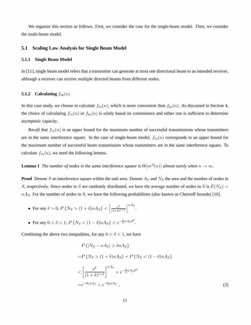
Lemma 1 The number of nodes in the same interference square is Θ(nr2(n)) almost surely when n → ∞.

Proof DenoteS an interference square within the unit area. DenoteAS andNS the area and the number of nodes in

S, respectively. Since nodes inS are randomly distributed, we have the average number of nodes inS is E(NS) =

nAS . For the number of nodes inS, we have the following probabilities (also known as Chernoff bounds) [10].

• For anyδ > 0, P NS > (1 + δ)nAS <[

eδ

(1+δ)1+δ

]nAS

.

• For any0 < δ < 1, P NS < (1− δ)nAS < e−12nASδ

2.

Combining the above two inequalities, for any0 < δ < 1, we have

P |NS − nAS| > δnAS

=P NS > (1 + δ)nAS+ P NS < (1− δ)nAS

<

[

eδ

(1 + δ)1+δ

]nAS

+ e−12nASδ

2

=e−θ1nAS + e−θ2nAS , (2)

11

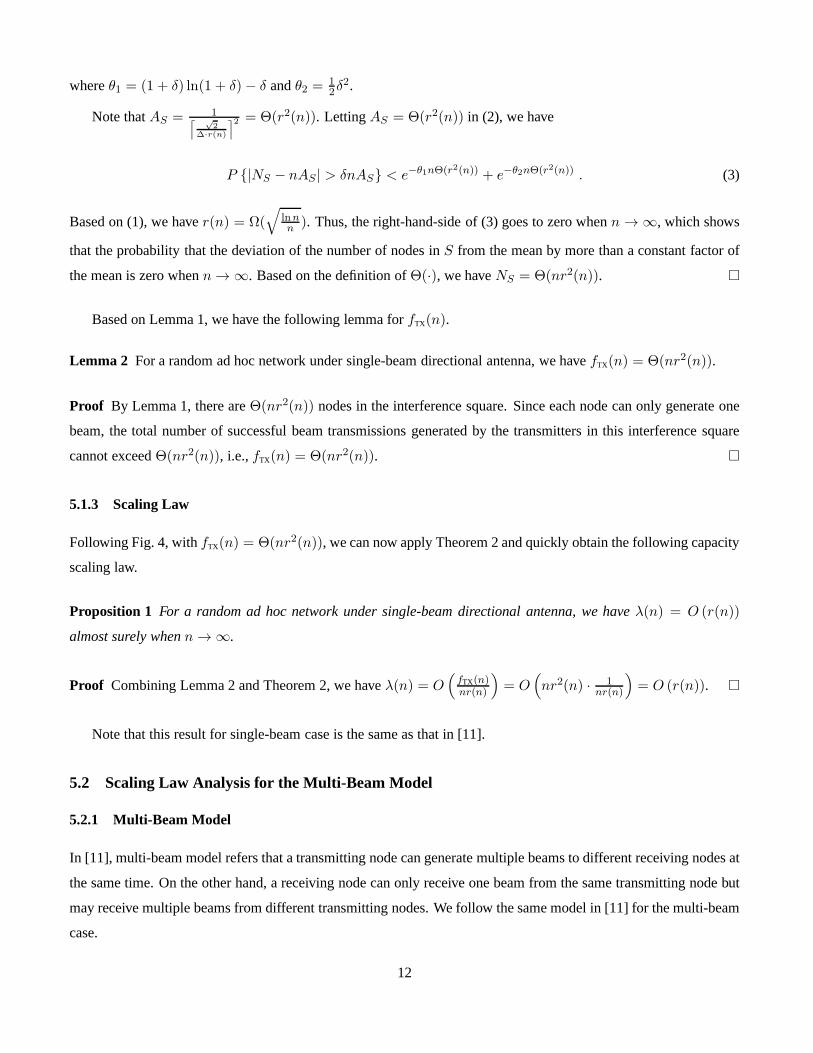
whereθ1 = (1 + δ) ln(1 + δ)− δ andθ2 = 12δ

2.

Note thatAS = 1⌈ √

2∆·r(n)

⌉2 = Θ(r2(n)). LettingAS = Θ(r2(n)) in (2), we have

P |NS − nAS | > δnAS < e−θ1nΘ(r2(n)) + e−θ2nΘ(r2(n)) . (3)

Based on (1), we haver(n) = Ω(√

lnnn). Thus, the right-hand-side of (3) goes to zero whenn → ∞, which shows

that the probability that the deviation of the number of nodes inS from the mean by more than a constant factor of

the mean is zero whenn → ∞. Based on the definition ofΘ(·), we haveNS = Θ(nr2(n)).

Based on Lemma 1, we have the following lemma forfTX(n).

Lemma 2 For a random ad hoc network under single-beam directional antenna, we havefTX(n) = Θ(nr2(n)).

Proof By Lemma 1, there areΘ(nr2(n)) nodes in the interference square. Since each node can only generate one

beam, the total number of successful beam transmissions generated by the transmitters in this interference square

cannot exceedΘ(nr2(n)), i.e.,fTX(n) = Θ(nr2(n)).

5.1.3 Scaling Law

Following Fig. 4, withfTX(n) = Θ(nr2(n)), we can now apply Theorem 2 and quickly obtain the following capacity

scaling law.

Proposition 1 For a random ad hoc network under single-beam directional antenna, we have λ(n) = O (r(n))

almost surely when n → ∞.

Proof Combining Lemma 2 and Theorem 2, we haveλ(n) = O(

fTX(n)nr(n)

)

= O(

nr2(n) · 1nr(n)

)

= O (r(n)).

Note that this result for single-beam case is the same as thatin [11].

5.2 Scaling Law Analysis for the Multi-Beam Model

5.2.1 Multi-Beam Model

In [11], multi-beam model refers that a transmitting node can generate multiple beams to different receiving nodes at

the same time. On the other hand, a receiving node can only receive one beam from the same transmitting node but

may receive multiple beams from different transmitting nodes. We follow the same model in [11] for the multi-beam

case.

12

∆

+! "∆! "

Figure 5: The larger square contains all the transmitters that can transmit directional beams to the receivers that are

in the small interference square at the center.

5.2.2 Calculating fRX(n)

We will calculatefRX(n).3 Recall thatfRX(n) is an upper bound of the maximum number of successful transmissions

whose receivers are in the same interference square. In the case of multi-beam model,fRX(n) corresponds to an

upper bound of the maximum number of successful beam transmissions received by the receivers that are in the

same interference square.

For receivers residing in the same interference square, it is easy to see that their transmitters cannot be outside a

larger square, with the same center as the interference square, but with side length of1/⌈√2

∆·r(n)⌉+2r(n) (see Fig. 5).

Otherwise, a receiver in the interference square will be outside of a transmitter’s transmission ranger(n). For the

number of nodes inside the larger square (regardless of transmitters or receivers), we have the following lemma.

Lemma 3 The number of nodes in the larger square with side length 2r(n) + 1⌈ √

2∆·r(n)

⌉ is Θ(nr2(n)) almost surely

when n → ∞.

The proof of Lemma 3 is similar to the proof of Lemma 1 and is omitted here. Now, we are ready to calculate

fRX(n) as follows.

Lemma 4 For a random ad hoc network under multi-beam directional antenna, we have fRX(n) = O(n2r4(n)).

3The level of difficulty in calculatingfRX(n) is the same asfTX(n) for the multi-beam model. Either choice will lead to the sameresult.

13

Proof Based on Lemma 3, we know that the number of transmitters thatcan transmit beams to the same receiver

in the interference square is at mostO(nr2(n)). That is, a receiver in the interference square can receive at most

O(nr2(n)) beams. By Lemma 1, there are at mostΘ(nr2(n)) receivers in the same interference square. So we have

fRX(n) = Θ(nr2(n)) ·O(nr2(n)) = O(n2r4(n)).

5.2.3 Scaling Law

Following Fig. 4, withfRX(n) = O(n2r4(n)), we can now apply Theorem 1 and quickly obtain the following

capacity scaling law.

Proposition 2 For a random ad hoc network under multi-beam directional antenna, we have λ(n) = O(

nr3(n))

almost surely when n → ∞.

Proof Combining Lemma 4 and Theorem 1, we haveλ(n) = O(

fRX(n)nr(n)

)

= O(

n2r4(n) · 1nr(n)

)

= O(

nr3(n))

.

This result is the same as that in [11] for the multi-beam case.

6 Case Study II: MIMO Ad Hoc Networks

6.1 MIMO Model

By employing multiple antennas at both transmitting and receiving nodes, MIMO has brought significant benefits

to wireless communications, such as increased link capacity [2, 16], improved link diversity [23], and interference

cancellation between conflicting links [1, 15]. In this section, we characterize asymptotic capacity for multi-hop

MIMO ad hoc networks. Although there are many schemes to exploit the benefits of antenna arrays at a node,

we focus on the two key characteristics of MIMO:spatial multiplexing and interference cancellation [1, 15, 22].

Spatial multiplexing refers that a transmitter can send several independent data streams to its intended receiver

simultaneously on a link. Interference cancellation refers that by properly exploiting multiple antennas at a node,

potential interference to and/or from other nodes can be cancelled.

To model spatial multiplexing and interference cancellation, we employ recent advance in MIMO link model in

[13] by Shiet al. In this model, degree-of-freedom (DoF) is used to representresource at a MIMO node. Simply put,

the number of DoFs at a node is equal to the number of antennas,denoted asα, at the node. Denotezl the number

of active data streams on linkl in a time slot. Denote Tx(l) and Rx(l) the transmitter and the receiver of linkl,

respectively. To spatial multiplexzl data streams on linkl, we need to allocatezl (zl ≤ α) DoFs at both transmitter

Tx(l) and receiver Rx(l). To cancel interference from and/or to other nodes in the network, it is necessary to have

14

an ordered list for all nodes and allocate DoFs at each node following this order [13]. DenoteΠ(·) the mapping

between a node and its order in the node list. Suppose that link l is carryingzl data streams. DenoteIl andQl the

set of links that are interfered by linkl and the set of links that are interfering linkl, respectively. Transmitter Tx(l)

is responsible for cancelling the interference from itselfto all receivers Rx(k), k ∈ Il, that are before node Tx(l) in

the order list. Similarly, receiver Rx(l) of link l is responsible for cancelling the interference from all transmitters

Tx(k), k ∈ Ql, that are before node Rx(l) in the order list. Since the total number of DoFs for spatial multiplexing

and interference cancellation cannot exceedα, we have the following two constraints on each active linkl in the

network.

1. DoF constraint at Tx(l): The number of DoFs that Tx(l) can use for spatial multiplexing (for transmission)

and interference cancellation cannot exceed the total number of DoFs at node Tx(l), i.e.,

zl +

Π(Tx(l))>Π(Rx(k))∑

k∈Il

zk ≤ α . (4)

2. DoF constraint at Rx(l): The number of DoFs that receiver Rx(l) can use for spatial multiplexing (for recep-

tion) and interference cancellation cannot exceed the total number of DoFs at node Rx(l), i.e.,

zl +

Π(Rx(l))>Π(Tx(k))∑

k∈Ql

zk ≤ α . (5)

We use the following simple example to illustrate DoF allocation in a MIMO network.

Example 2 Consider the three-link (k, l, andm) example in Fig. 6(a). The number of antennas at each node is also

shown in the figure. Under the above MIMO model, we need an order to determine the DoF resource usage at each

node. Suppose we are following an order list, saya → d → b → c → e → f among the nodes. Then, the DoF

allocation in this MIMO network works as follows.

We start with nodea, which is the first node in the list. Given it is the first in the list, nodea does not have any

interference with which it needs to be concerned. Since nodea has only 1 antenna, it can transmit at most 1 data

stream to its intended receiverb. The second node on the ordered list is noded. Since it appears in the order list

after nodea, noded needs to suppress the interference froma. This implies that noded needs to expend 1 DoF

to cancel the interference froma. Sinced has 2 antennas, we have thatd can receive at most2 − 1 = 1 stream,

i.e., zl ≤ 1. The DoF consumption on nodesb andc follows exactly the same token, and it can be verified thatb

andc can each receive and transmit 1 stream, respectively. Sincenodee’s transmission should not interfere with the

reception atb andd that had appeared in the order list earlier,e needs to expend 2 DoFs for this purpose. At this

point, e can transmit up to4 − 1 − 1 = 2 streams, i.e.,zm ≤ 2. Finally, along the same line, nodef can receive at

15

Link m

a

c

e

b

d

f

1 antenna1 antenna

2 antennas

4 antennas 4 antennas

2 antennas

Link k

Link l

(a) Inter-nodal interference relationship for three links.

zk

1 2 3 4

1

2

3

4

1

3

4

0

zl

zm

2

(b) Achievable DoF region of the three links.

Figure 6: A three-link network example.

most4 − 1 − 1 = 2 streams, i.e.,zm ≤ 2. Therefore, after the above steps, we can see that the streamcombination

(zk = 1, zl = 1, zm = 2) can be scheduled feasibly on linksk, l, andm. It can be shown that the entire DoF region

(the set of all feasible stream combinations) for the three-link example in Fig. 6(a) can be found by enumerating all

possible choices of the node order list. Each stream combination offers a feasible point (e.g.,(1, 1, 2)), the union of

which constitutes the DoF region, which we plot in Fig. 6(b).

6.2 Calculating fRX(n)

Based on the MIMO network model, we now calculatefRX(n).4 Recall thatfRX(n) is an upper bound of the maxi-

mum number of successful transmissions whose receivers arein the same interference square. In the case of MIMO,

this corresponds to the maximum number of successful data streams on all active links whose receivers are in the

same interference square.

Lemma 5 For a random MIMO ad hoc network, we have fRX(n) = α.

Proof DenoteL the set of active links with their receivers being in the sameinterference square. Denote|L| the

number of links inL, and letL = 1, . . . , |L|. Our goal is to find an upper bound for the sum of data streams on

these links, i.e.,∑

k∈L zk.

If |L| = 1, i.e., only one active link with its receiver in the interference square, thenz1 ≤ α (since the number

of data streams on this link cannot exceed the number DoFs of anode). We can setfRX(n) = α and the lemma holds

4For MIMO, the level of difficulty in calculatingfRX(n) is the same asfTX(n) and either approach will yield the same result.

16

trivially.

For the general scenario when|L| ≥ 2, Property 1 says that these|L| links interfere with each other and

interference cancellation is necessary. Based on the MIMO model we discussed earlier, we need to follow an

ordered list for the nodes (both transmitters and receivers) on these|L| links for DoF allocation at each node. We

have two cases, depending on whether the last node in the listis a transmitter or a receiver.

Case (i). The last node in the ordered list is a receiver. Without loss of generality, denotem as the link of which this

node is the receiver. To havezm data streams on linkm, based on (5), we have the following constraint on receiver

Rx(m).

zm +

Π(Rx(m))>Π(Tx(k))∑

k∈Qm

zk ≤ α , (6)

where the sum forzk is taken over all interfering links whose transmitters are before receiver Rx(m) in the node

list. Since linkm is being interfered by all other links inL in the same interference square, we haveQm = L\m.

Further, since Rx(m) is the last node in this list, we haveΠ(Rx(m)) > Π(Tx(k)), for all k ∈ L\m. Therefore,

(6) can be re-written as

zm +∑

k∈L\mzk ≤ α ,

which is∑

k∈Lzk ≤ α .

Thus, we have shown that the sum of data streams that can be received by nodes in the interference square over all

links is upper bounded byα, i.e.,fRX(n) = α.

Case (ii). The last node in the ordered list is a transmitter. In this case, we employ (4) and follow the same token as

the above discussion. We again havefRX(n) = α.

Combining the two cases, we conclude thatfRX(n) = α.

6.3 Scaling Law

Following Fig. 4, withfRX(n) = α, we can now apply Theorem 1 and obtain capacity scaling law ofa random

MIMO ad hoc network as follows.

Proposition 3 For a random MIMO ad hoc network, we have λ(n) = O(

1√n lnn

)

almost surely when n → ∞.

This result is the same as that in [7]. It is also interesting to see that, despite MIMO’s ability to increase capacity

in a finite-sized network, the scaling order for its asymptotic capacity remains the same as that for the classical single

omnidirectional antenna network as in [4].

17

7 Case Study III: Multi-Channel and Multi-Radio

7.1 Multi-Channel Multi-Radio Model

Multi-channel multi-radio (MC-MR) refers that there are multiple channels in the network and there are multiple

radio interfaces at each node in the network [8, 9]. By equipping each node with multiple radio interfaces, each

node has more flexibility in accessing the multiple channelsin the network. Following [8], we assume that there

arec channels in the network and each node in the network is equipped withm radio interfaces, wherec andm are

constants, and1 ≤ m ≤ c. A radio interface is capable of transmitting or receiving data on only one channel at any

given time, i.e., half-duplex.

7.2 Calculating fRX(n)

Based on the MC-MR model, we now calculatefRX(n).5 Assuming each band has the same bandwidth in the

MC-MR network, thenfRX(n) corresponds to the maximum number of successful transmissions over all available

channels on all radio interfaces whose receivers are in the same interference square. We have the following lemma.

Lemma 6 For a random MC-MR network, we have fRX(n) = c.

Proof Let’s focus on one channel at a time. Since the links with receivers in the interference square interfere with

each other (Property 1), there can be at most one radio at a node receiving on this channel. Summing up all such

radios (or successful transmissions) overc channels, we havefRX(n) = c.

7.3 Scaling Law

Following Fig. 4, withfRX(n) = c, we can now apply Theorem 1 and obtain capacity scaling law ofan MC-MR ad

hoc network as follows.

Proposition 4 For a random MC-MR ad hoc network, we have λ(n) = O(

1√n lnn

)

almost surely when n → ∞.

Note that this result is the same as the result in [8] for the case whencm

= O(lnn).

8 Case Study IV: Cognitive Radio Ad Hoc Networks

8.1 Cognitive Radio Network Model

Cognitive radio (CR) is another new physical layer technology that enables more efficient utilization of radio spec-

trum [19]. A CR is able to constantly sense the radio spectrumand explore any available spectrum bands for data5For an MC-MR network, the level of difficulty in calculatingfRX(n) is the same asfTX(n) and either approach will yield the same result.

18

communication. Consider a random ad hoc network where each node is equipped with a CR. Consider a specific

time instance where each nodei senses a set of available frequency bandsBi that it can use.6 Note that due to

differences in locations, the set of available frequency bandsBi at a nodei may not be identical to that of another

node in the network. DenoteBij = Bi

⋂Bj the set of common bands that are available at both nodesi andj. Then

nodei can communicate to nodej on bandm only if m ∈ Bij .

8.2 Calculating fRX(n)

Based on the CR network model, we now calculatefRX(n).7 Assuming each band has the same bandwidth in the

CR network, thenfRX(n) corresponds to the maximum number of successful transmissions over all available bands

whose receivers are in the same interference square. DenoteM = |⋃ni=1 Bi|, i.e., M is the number of distinct

frequency bands in the network. Then we have the following lemma.

Lemma 7 For a random CR ad hoc network, we have fRX(n) = M .

Proof Consider one band at a time. Within each band, by Property 1, the links with receivers in the interference

square interfere with each other. So the maximum number of active links (or successful transmissions) is at most

one. Summing up all active links (or successful transmissions) overM bands, we havefRX(n) = M .

8.3 Scaling Law

Following Fig. 4, withfRX(n) = M , we can now apply Theorem 1 and obtain capacity scaling law ofa random CR

ad hoc network as follows.

Proposition 5 For a random CR ad hoc network, we have λ(n) = O(

1√n lnn

)

almost surely when n → ∞.

This result is consistent to those found in [5, 14]. It is interesting to see that, despite that CR can utilize spectrum

bands more efficiently (and thus higher capacity for a finite-sized network), the scaling order of its asymptotic

capacity remains the same as that for the classical single omnidirectional antenna network in [4].

9 Case Study V: Ad Hoc Networks with Multi-Packet Reception

Multi-packet reception (MPR) is a conceptual abstraction of a physical layer capability that a receiver can correctly

decode multiple packets from different transmitters simultaneously [17]. As described in [12], such capability may

be implemented by a variety of advanced physical layer technologies, such as multiuser detection [18], directional

6These bands may be those that are currently unused by the primary users.7For a CR network, the level of difficulty in calculatingfRX(n) is the same asfTX(n) and either approach will yield the same result.

19

antennas [11, 20], and MIMO. In other words, MPR refers to a reception capability of a node at the physical layer,

rather than referring to a specific physical layer technology. In this section, we employ our criteria in Section 4 to

explore capacity scaling law of MPR-based ad hoc networks.

9.1 The MPR Model

In the MPR model, a transmitter can transmit packet to only one receiver at a time, but a receiver is capable of

receiving multiple packets simultaneously from multiple transmitters within its transmission range. For unintended

transmissions whose interference range covers a receiver,the receiver will consider them as interference. Such

interference may be cancelled by the receiver. Specifically, in the MPR model, we assume a receiver has finite

resource available for multi-packet reception and interference cancellation. Denoteβ1 the number of simultaneous

packets from intended transmitters whose transmission range covers the receiver andβ2 the number of unintended

transmitters that produce interference on the same receiver. We have

β1 + β2 ≤ β ,

whereβ is a constant and represents the total available resource ata receiver. For example, if MIMO is employed to

implement MPR, then the number of DoFs at a MIMO node may correspond toβ.

Note that this MPR model is a generalization of the idealizedMPR model in [12] which assumesβ1 ≤ β = ∞andβ2 = 0, i.e., a receiver can successfully decode arbitrary numberof simultaneous packet transmissions and no

interference is allowed on the receiver.

9.2 Calculating fRX(n)

We choose to calculatefRX(n), which is more convenient than calculatingfTX(n). Recall thatfRX(n) is an upper

bound of the maximum number of successful transmissions whose receivers are in the same interference square. In

the case of MPR ad hoc networks,fRX(n) corresponds to an upper bound of the maximum number of packets that

are successfully received simultaneously by all the receivers in the same interference square. We have the following

lemma forfRX(n).

Lemma 8 For a random MPR ad hoc network, we have fRX(n) = β.

Proof DenoteL the set of successful links with their receivers residing inthe same interference square. By a

“successful” link, we mean the receiver of this link can successfully decode the packet on this link. Denote|L| the

number of links inL, and letL = 1, . . . , |L|. ThenfRX(n) is an upper bound of|L|.Note that for two successful links, their transmitters are different but their receivers may be the same. Consider

one receiverj in the interference square. From receiverj’s perspective, we divideL into two subsets:L1 — the set

20

Table 2: Summary of capacity scaling laws obtained via our simple criteria for different physical layer technologies.

“—” sign indicates new result not yet available in the literature.

Physical Layer Technology fRX(n) or fTX(n) Upper Bound Reference

Directional antennaSingle beam fTX(n) = Θ(nr2(n)) O(r(n)) [11]Multi-beam fRX(n) = O(n2r4(n)) O(nr3(n)) [11]

MIMO fRX(n) = α O(1/√n lnn) [7]

MC-MR fRX(n) = c O(1/√n lnn) [8]

CR fRX(n) = M O(1/√n lnn) [5, 14]

MPRIdealized fRX(n) = Θ(nr2(n)) O(r(n)) [12]General fRX(n) = β O(1/

√n lnn) —

of links whose receivers arej, andL2 — the set of links whose receivers are notj. Based on Property 1, we know

that the transmitters of the links in subsetL2 are all in the interference range of receiverj. Since packets onL1 are

successfully received byj, then based on the MPR model, we have

|L| = |L1|+ |L2| = β1 + β2 ≤ β .

Therefore, we havefRX(n) = β.

9.3 Scaling Law

Following Fig. 4, withfRX(n) = β, we can now apply Theorem 1 and directly obtain the followingcapacity scaling

law for an MPR-based ad hoc network.

Proposition 6 For a random MPR ad hoc network, we have λ(n) = O(

1/√n lnn

)

almost surely when n → ∞.

Remark 1 For the idealized MPR model described in [12], whereβ1 ≤ β = ∞ andβ2 = 0, one can still apply our

simple scaling order criteria. In particular, it can be shown that for this idealized MPR model,fRX(n) = Θ(nr2(n))

(see the appendix for details). By Theorem 1, we haveλ(n) = O(

fRX(n)nr(n)

)

= O(

nr2(n) · 1nr(n)

)

= O (r(n)). This

is exactly the result developed in [12].

10 Discussions

Summary of Results. Table 2 summarizes capacity scaling laws (upper bounds) that we explored in Sections 5

to 9 by applying our simple scaling order criteria. These upper bounds are the same as those studied in previous

work (last column in Table 2), which were developed by various custom-designed approaches. For the MPR general

model, there is no prior result available in the literature.

21

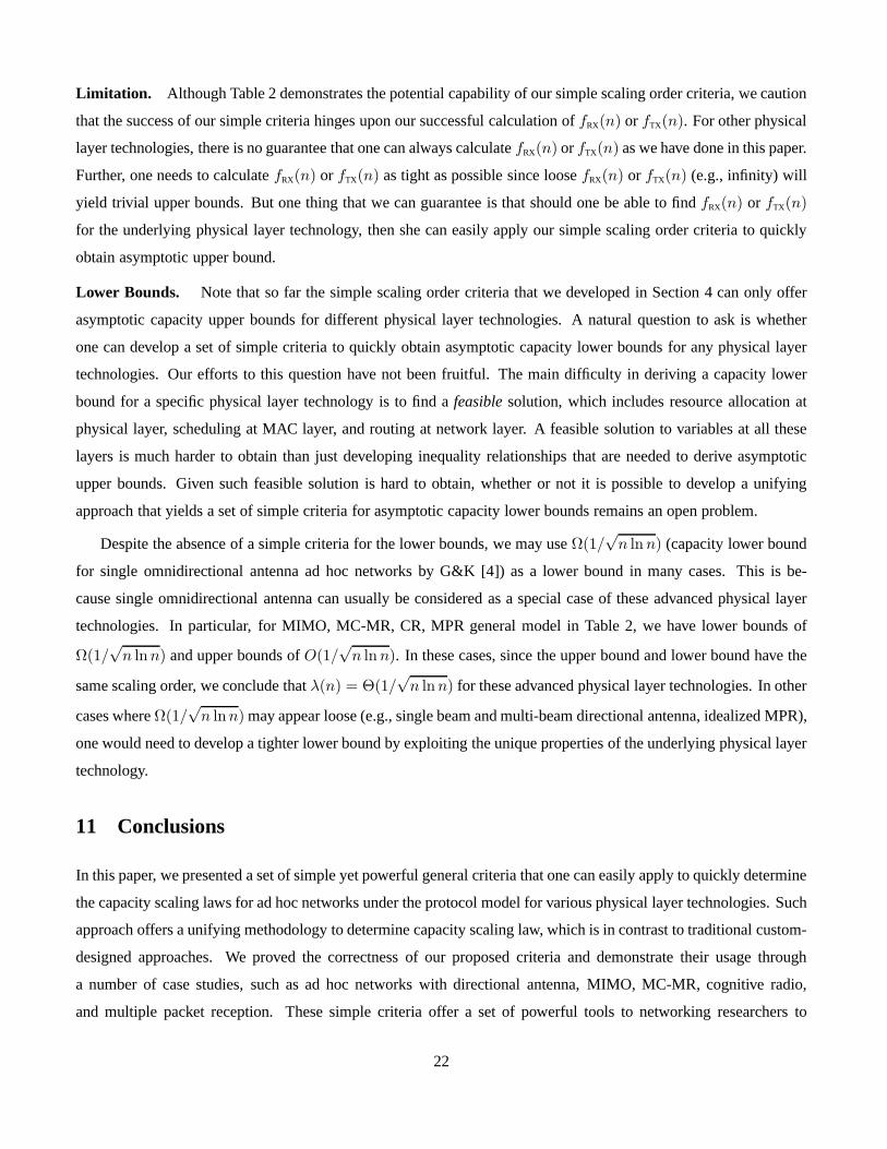
Limitation. Although Table 2 demonstrates the potential capability of our simple scaling order criteria, we caution

that the success of our simple criteria hinges upon our successful calculation offRX(n) or fTX(n). For other physical

layer technologies, there is no guarantee that one can always calculatefRX(n) or fTX(n) as we have done in this paper.

Further, one needs to calculatefRX(n) or fTX(n) as tight as possible since loosefRX(n) or fTX(n) (e.g., infinity) will

yield trivial upper bounds. But one thing that we can guarantee is that should one be able to findfRX(n) or fTX(n)

for the underlying physical layer technology, then she can easily apply our simple scaling order criteria to quickly

obtain asymptotic upper bound.

Lower Bounds. Note that so far the simple scaling order criteria that we developed in Section 4 can only offer

asymptotic capacity upper bounds for different physical layer technologies. A natural question to ask is whether

one can develop a set of simple criteria to quickly obtain asymptotic capacity lower bounds for any physical layer

technologies. Our efforts to this question have not been fruitful. The main difficulty in deriving a capacity lower

bound for a specific physical layer technology is to find afeasible solution, which includes resource allocation at

physical layer, scheduling at MAC layer, and routing at network layer. A feasible solution to variables at all these

layers is much harder to obtain than just developing inequality relationships that are needed to derive asymptotic

upper bounds. Given such feasible solution is hard to obtain, whether or not it is possible to develop a unifying

approach that yields a set of simple criteria for asymptoticcapacity lower bounds remains an open problem.

Despite the absence of a simple criteria for the lower bounds, we may useΩ(1/√n lnn) (capacity lower bound

for single omnidirectional antenna ad hoc networks by G&K [4]) as a lower bound in many cases. This is be-

cause single omnidirectional antenna can usually be considered as a special case of these advanced physical layer

technologies. In particular, for MIMO, MC-MR, CR, MPR general model in Table 2, we have lower bounds of

Ω(1/√n lnn) and upper bounds ofO(1/

√n lnn). In these cases, since the upper bound and lower bound have the

same scaling order, we conclude thatλ(n) = Θ(1/√n lnn) for these advanced physical layer technologies. In other

cases whereΩ(1/√n lnn) may appear loose (e.g., single beam and multi-beam directional antenna, idealized MPR),

one would need to develop a tighter lower bound by exploitingthe unique properties of the underlying physical layer

technology.

11 Conclusions

In this paper, we presented a set of simple yet powerful general criteria that one can easily apply to quickly determine

the capacity scaling laws for ad hoc networks under the protocol model for various physical layer technologies. Such

approach offers a unifying methodology to determine capacity scaling law, which is in contrast to traditional custom-

designed approaches. We proved the correctness of our proposed criteria and demonstrate their usage through

a number of case studies, such as ad hoc networks with directional antenna, MIMO, MC-MR, cognitive radio,

and multiple packet reception. These simple criteria offera set of powerful tools to networking researchers to

22

understand throughput scaling behavior of ad hoc networks under different physical layer technologies, particularly

new technologies that will appear in the future.

References

[1] L.-U. Choi and R.D. Murch, “A transmit preprocessing technique for multiuser MIMO systems using a decomposition

approach,”IEEE Trans. on Wireless Commun., vol. 3, no. 1, pp. 20–24, Jan. 2004.

[2] G.J. Foschini, “Layered space-time architecture for wireless communication in a fading environment when using multi-

element antennas,”Bell Labs Technical Journal, vol. 1, no. 2, pp. 41–59, Autumn 1996.

[3] P. Gupta and P.R. Kumar, “Critical power for asymptotic connectivity in wireless networks,” inStochastic Analysis,

Control, Optimization and Applications: A Volume in Honor of W.H. Fleming, W.M. McEneany, G. Yin, and Q. Zhang,

Eds. Boston, MA: Birkhauser, pp. 547–566, 1998.

[4] P. Gupta and P. Kumar, “The capacity of wireless networks,” IEEE Transactions on Information Theory, vol. 46, no. 2,

pp. 388–404, March 2000.

[5] W. Huang and X. Wang, “Throughput and delay scaling of general cognitive networks,” inProc. IEEE INFOCOM,

pp. 2210-2218, Shanghai, China, Apr. 2011.

[6] S.-W. Jeon, N. Devroye, M. Vu, S.-Y. Chung, and V. Tarokh,“Cognitive networks achieve throughput scaling of a

homogeneous network,” inProc. 7th Intl. Symposium on Modeling and Optimization in Mobile, Ad Hoc, and Wireless

Networks (WiOpt), 5 pages, Seoul, Korea, June 2009.

[7] C. Jiang, Y. Shi, Y.T. Hou, and S. Kompella, “On the asymptotic capacity of multi-hop MIMO ad hoc networks,”IEEE

Trans. on Wireless Commun., vol. 10, no. 4, pp. 1032–1037, Apr. 2011.

[8] P. Kyasanur and N.H. Vaidya, “Capacity of multi-channelwireless networks: Impact of number of channels and inter-

faces,” inProc. ACM MobiCom, pp. 43–57, Cologne, Germany, Aug. 28–Sep. 2, 2005.

[9] M. Kodialam and T. Nandagopal, “Characterizing the capacity region in multi-radio multi-channel wireless mesh net-

works,” in Proc. ACM MobiCom, pp. 73–87, Cologne, Germany, Aug. 28–Sep. 2, 2005.

[10] R. Motwani and P. Raghavan,Randomized Algorithms, Chapter 4, Cambridge University Press, 1995.

[11] C. Peraki and S.D. Servetto, “On the maximum stable throughput problem in random networks with directional antennas,”

in Proc. ACM MobiHoc, pp. 76–87, Annapolis, MD, June 1–3, 2003.

[12] H.R. Sadjadpour, Z. Wang, and J.J. Garcia-Luna-Aceves, “The capacity of wireless ad hoc networks with multi-packet

reception,”IEEE Trans. on Commun., vol. 58, no. 2, pp. 600–610, Feb. 2010.

[13] Y. Shi, J. Liu, C. Jiang, C. Gao, and Y.T. Hou, “An optimallink layer model for multi-hop MIMO networks,” inProc.

IEEE INFOCOM, pp. 1916–1924, Shanghai, China, Apr. 2011.

23

[14] Y. Shi, C. Jiang, Y.T. Hou, and S. Kompella, “On capacityscaling law of cognitive radio ad hoc networks (Invited Paper),”

in Proc. IEEE ICCCN, Maui, Hawaii, July 31–Aug. 4, 2011.

[15] Q.H. Spencer, A.L. Swindlehurst, and M. Haardt, “Zero-forcing methods for downlink spatial multiplexing in multiuser

MIMO channels,”IEEE Trans. on Signal Process., vol. 52, no. 2, pp. 388–404, Feb. 2004.

[16] I.E. Telatar, “Capacity of multi-antenna Gaussian channels,” European Transactions on Telecommunications, vol. 10,

no. 6, pp. 585–596, Nov. 1999.

[17] L. Tong, Q. Zhao and G. Mergen, “Multipacket reception in random access wireless networks: From signal processing to

optimal medium access control,”IEEE Communications Magazine, vol. 39, no. 11, pp. 108–112, Nov. 2001.

[18] S. Verdu,Multiuser Detection, Cambridge Univ. Press, 1998.

[19] A.M. Wyglinski, M. Nekovee, and Y.T. Hou (Editors),Cognitive Radio Communications and Networks: Principles and

Practices, Academic Press/Elsevier, 2010.

[20] S. Yi, Y. Pei, and S. Kalyanaraman, “On the capacity improvement of ad hoc wireless networks using directional anten-

nas,” inProc. ACM MobiHoc, pp. 108–116, Annapolis, MD, June 1–3, 2003.

[21] C. Yin, L. Gao, and S. Cui, “Scaling laws of overlaid wireless networks: A cognitive radio network vs. a primary network,”

IEEE/ACM Trans. on Networking, vol. 18, no. 4, pp. 1317–1329, Aug. 2010.

[22] T. Yoo and A. Goldsmith, “On the optimality of multiantenna broadcast scheduling using zero-forcing beamforming,”

IEEE J. Selected Areas in Commun., vol. 24, no. 3, pp. 528–541, March 2006.

[23] L. Zheng and D.N.C. Tse, “Diversity and multiplexing: Afundamental tradeoff in multiple-antenna channels,”IEEE

Trans. on Information Theory, vol. 49, no. 5, pp. 1073–1096, May 2003.

Appendix

Proof of Theorem 1 Recall that we divide the unit square into small interference squares with each having a side

length of1/⌈√2

∆·r(n)⌉ (see Fig. 2). DenotefRX(n) an upper bound of the maximum number of successful transmissions

whose receivers are in the same interference square. Then, the total data rate that each interference square can support

is at mostfRX(n)W . Now, we can compute the maximum data rate that can be supported by the network in the unit

square by taking the sum of the data rates among all small interference squares. Since the side length of each small

interference square is1/⌈√2

∆·r(n)⌉, the total number of small interference squares in the unit area is⌈√2

∆·r(n)⌉2. So the

maximum data rate that can be supported in the network is at most ⌈√2

∆·r(n)⌉2fRX(n)W .

Let D be the average distance between a source node and its destination node. Since multi-hop routing is

employed, we have that the average number of hops for each source-destination pair is at leastDr(n) . Note that there

aren source-destination pairs. Thus, the required transmission rate over the entire network is at leastDr(n)nλ(n).

24

Since the maximum data transmission that can be supported inthe network at a time is⌈√2

∆·r(n)⌉2fRX(n)W , we

have Dr(n)nλ(n) ≤ ⌈

√2

∆·r(n)⌉2fRX(n)W < (√2

∆·r(n) + 1)2fRX(n)W, which gives us

λ(n) <2fRX(n)W

∆2Dnr(n)+

2√2fRX(n)W

∆Dn+

fRX(n)Wr(n)

Dn= O

(

fRX(n)

nr(n)

)

. (7)

This proves the first part of Theorem 1.

Now, we show the special case whenfRX(n) is a constant. In this case, based on (7), we have

λ(n) = O

(

1

nr(n)

)

. (8)

Note that based on (1), we haver(n) ≥√

lnnn

. By substitutingr(n) =√

lnnn

into (8), we have

λ(n) = O

1

n√

lnnn

= O

(

1√n lnn

)

.

Calculating fRX(n) for idealized MPR model. We obtainfRX(n) as follows.

Lemma 9 For a random ad hoc network under the idealized MPR model, we have fRX(n) = Θ(nr2(n)).

Proof First, we show that there can be only one receiver (sayj) in the interference square receiving packets. This

can be shown by contradiction. Suppose there is another receiver i, i 6= j, in the same interference square receiving

packets. Then, based on Property 1, a transmitter to receiver i is within the interference range of nodej. This

transmitter of receiveri will bring interference at nodej, which contradicts withβ2 = 0 under the idealized MPR

model.

Although there is only one receiverj receiving packets, it may receive packets from multiple transmitters. Note

that all nodes that can transmit to receiverj must fall within the larger square with a side length of1/⌈√2

∆·r(n)⌉+2r(n)

(see Fig. 5). Based on Lemma 3, we know that the number of all nodes inside the larger square isΘ(nr2(n)). Since

each transmitter transmits one packet to receiverj at a time, the number of simultaneous packets received by receiver

j cannot exceed the number of nodes in the larger square, i.e.,Θ(nr2(n)). Therefore, we havefRX(n) = Θ(nr2(n)).

25