Toward an Understanding of the Built Environment Influences on the Carpool Formation and Use Process: A Case Study of Employer-based Users within the Service

Sector of Smart Commute’s Carpool Zone

by

Randy Bui

A thesis submitted in conformity with the requirements for the degree of Master of Science

Department of Geography & Program in Planning University of Toronto

© Copyright by Randy Bui 2011

ii

Toward an Understanding of the Built Environment Influences on

the Carpool Formation and Use Process: A Case Study of

Employer-based Users within the Service Sector of Smart

Commute’s Carpool Zone

Randy Bui

Master of Science

Department of Geography & Program in Planning University of Toronto

2011

Abstract

The recent availability of geo-enabled web-based tools creates new possibilities for facilitating

carpool formation. Carpool Zone is a web-based carpool formation service offered by Metrolinx,

the transportation planning authority for the Greater Toronto and Hamilton Area (GTHA),

Canada. The carpooling literature has yet to uncover how different built environments may

facilitate or act as barriers to carpool propensity. This research explores the relationship between

the built environment and carpool formation.

With respect to the built environment, industrial and business parks (homogeneous land-

use mix) are associated with high odds of forming carpools. The results suggest that employer

transport policies are also among the more salient factors influencing carpool formation and use.

Importantly, the findings indicate that firms interested in promoting carpooling will require

contingencies to reduce the uncertainty of ride provision that may hamper long-term carpool

adoption by employees.

iii

Acknowledgments

The completion of this thesis would not have been possible without the contribution,

support and guidance of several individuals. First and foremost, my deepest gratitude goes to Dr.

Ron Buliung who has supervised me throughout my Undergraduate and Master theses. Ron, I

sincerely thank you for your guidance and patience throughout these years. Without your

continued confidence in me, I would have never achieved the success so far in my academic

career. Secondly, I like to thank my committee members (Dr. Joseph Leydon & Dr. Pierre

Desrochers) for their participation in my defense and providing me with meaningful feedback.

I also would like to acknowledge Ryan Lanyon from Metrolinx for providing assistance

and funding support to carry out this research. Thank you for giving me the opportunity to be

involved in a project that has made me a more conscious commuter.

I would like to express my sincere gratitude to the donors and the Department of

Geography for awarding me the Ontario Graduate Scholarship in Science and Technology (ESRI

Canada Scholarship).

I’d like to extend my thanks to friends, fellow grad students, and the supportive

administrative staff of the Department of Geography at the University of Toronto Mississauga.

Finally, I sincerely thank my parents, Anh Huynh and Vinh Bui, for providing me with

support throughout my entire life.

iv

Table of Contents

Table of Contents

Acknowledgments ................................................................................................................................ iii

Table of Contents .................................................................................................................................. iv

List of Tables ........................................................................................................................................ vi

List of Figures ...................................................................................................................................... vii

1 Introduction ....................................................................................................................................... 1

1.1 Carpooling in North America .................................................................................................... 5

1.2 Defining Carpooling .................................................................................................................. 6

1.3 History of Carpooling .............................................................................................................. 10

1.4 Research Objectives ................................................................................................................ 13

1.5 Outline of Thesis ..................................................................................................................... 13

2 Literature Review ........................................................................................................................... 14

2.1 Socio-economic & Demographic Characteristics ................................................................... 15

2.2 Motivation for Carpooling ...................................................................................................... 17

2.3 Workplace Characteristics ....................................................................................................... 18

2.4 Household Auto-Mobility ....................................................................................................... 18

2.5 Commute Distance .................................................................................................................. 19

2.6 Scheduling of Work ................................................................................................................ 20

2.7 Role Preference ....................................................................................................................... 21

2.8 Links with Transportation Demand Management (TDM) ...................................................... 21

2.9 Built Environment ................................................................................................................... 22

2.10 Summary & Synthesis ............................................................................................................. 23

3 Study Area, Data, Methodology ..................................................................................................... 25

3.1 Study Area ............................................................................................................................... 26

v

3.2 Methods ................................................................................................................................... 30

3.2.1 Dataset, Data Limitations, Data Filtering ................................................................... 30

3.2.2 Model Specification .................................................................................................... 39

3.2.3 The Explanatory Variables Overview ......................................................................... 41

3.2.4 Spatial Modeling ......................................................................................................... 53

4 Results ............................................................................................................................................. 58

4.1 Sample Exploration ................................................................................................................. 58

4.1.1 Sample Geography ...................................................................................................... 58

4.1.2 Formed versus Non-Formed ....................................................................................... 61

4.2 Logistic Regression ................................................................................................................. 66

4.2.1 Bivariate Results ......................................................................................................... 67

4.2.2 Multivariate Results .................................................................................................... 72

4.3 Spatial Modeling ..................................................................................................................... 73

4.3.1 Carpool Hotspots ........................................................................................................ 74

4.3.2 Spatial Autocovariate Regression Results .................................................................. 79

5 Discussion ....................................................................................................................................... 82

5.1 Formed versus Non-formed .................................................................................................... 83

5.2 Logistic Regression Modeling ................................................................................................ 91

5.3 Carpooling Hotspots ................................................................................................................ 93

5.4 Spatial Modeling and Implications ......................................................................................... 97

6 Conclusions ................................................................................................................................... 100

6.1 Summary of Findings ............................................................................................................ 100

6.2 Policy Recommendations ...................................................................................................... 103

6.3 Future Research ..................................................................................................................... 104

References .......................................................................................................................................... 105

vi

List of Tables Table 1 Goods-Producing versus Services-Producing Industries ................................................. 33

Table 2 Variable Descriptions ...................................................................................................... 41

Table 3 Distribution of Respondents by Trip Destination in each Smart Commute TMA .......... 59

Table 4 Descriptive Statistics of Continuous Variables for Form and Non-Formed Groups ....... 63

Table 5 Descriptive Statistics of Categorical Variables for Form and Non-Formed Groups ....... 64

Table 6 Bivariate Regressions - Carpool Formation ..................................................................... 68

Table 7 Multivariate Regression - Carpool Formation ................................................................. 73

Table 8 Autocovariate Regression - Carpool Formation .............................................................. 81

vii

List of Figures Figure 1 Screenshot of Smart Commute's Carpool Zone Tool ....................................................... 5

Figure 2 TMA of Smart Commute ................................................................................................ 27

Figure 3 Golden Horseshoe (Outer) & Greater Toronto Hamilton Area (Inner) .......................... 28

Figure 4 Flowchart of Data Filter Process .................................................................................... 38

Figure 5 The Geography of Carpool Zone Users (Final Sample: n=358) .................................... 60

Figure 6 Comparison of Non-formed vs. Formed Kernel Density Maps ..................................... 62

Figure 7 Brampton Carpool Hotspot ............................................................................................. 76

Figure 8 North Eastern Toronto Carpool Hotspot ........................................................................ 77

Figure 9 Central Toronto Carpool Hotspot ................................................................................... 78

Figure 10 Sheridan Park Destinations – North Eastern Toronto Hotspot ..................................... 95

Figure 11 Bramalea City Centre Destinations– Brampton Hotspot .............................................. 97

1

1 Introduction The global passenger vehicle fleet is projected to increase from 800 million (in 2002) to over 2

billion motorized vehicles by 2030 (Dargay et al., 2007). The global demand for motorized

mobility is expected to intensify traffic congestion, energy demand, and environmental concerns.

In Canada, 83% of all households owned or leased at least one motor vehicle for their personal

use in 2006 (Statistics Canada, 2008a). The total number of vehicles registered in Ontario

increased by 12.53% between 1999 and 2007 (Statistics Canada, 2007). This rise in auto

ownership is also a concern to policymakers and planners in the Greater Golden Horseshoe,

Canada’s largest metropolitan area (Metrolinx, 2011a).

The substantial influx of automobiles on Canadian roadways has potentially negative

repercussions on the economy and the environment. A recent report by the Toronto Board of

Trade ranked Toronto last out of 21 major metropolitan cities in the world in terms of average

commute time (in minutes) for a trip to and from work. On average, Torontonians spend 80-

minutes on their round-trip journey to work each day (Toronto Board of Trade, 2011). The recent

steep rise in fuel prices is also a growing concern for consumers. The average yearly price for

regular gasoline in Ontario increased from 56.2 cents per litre in 1990 to 101.6 cents per litre by

the end of 2010 (Ontario Ministry of Energy, 2011). The Organization for Economic Co-

operation and Development estimates traffic congestion in Toronto cost roughly $3.3 billion

annually in lost productivity (OECD, 2010). With regard to environmental concerns, overall

transportation accounted for 26% of Canada's estimated GHG emissions in 2005, an increase of

33% from levels reported for 1990 (Environment Canada, 2007). The effects of rising fuel costs,

traffic congestion and long commute times have stimulated much attention from the public

toward sustainable transportation alternatives. One of these options is carpooling – defined as the

2

sharing of a private vehicle between two or more persons for work or school purposes (Teal,

1987). Understanding the process behind carpool formation and use may assist policymakers in

the development of effective strategies to increase carpooling, particular in support of travel

demand for the morning commute (Buliung et al., 2010).

The rising demand for on-road transportation (e.g., small/large cars, light passenger

trucks, motorcycles, school buses, urban transit) has outpaced that of other transport modes.

From 1990 to 2006, average on-road transportation energy demand increased by 0.9% per year in

Canada (National Energy Board, 2009). The increasing demand for passenger vehicles on

Canadian roadways is a problematic concern for traffic congestion and its negative externalities.

According to Statistics Canada (2008b), a large majority of Canadians (72.3%) are commuting to

work as a single occupant auto driver. With respect to travel time, the Transportation Tomorrow

Survey (TTS) found that the morning commute (6 - 9 am) within the Greater Toronto and

Hamilton Area (GTHA) accounts for 22.9% of all trips within a 24 hour period (Data

Management Group, 2009). Home-based work trips make up 48% of all trips, followed by home-

based school trips with 22%. The above figures illustrate the importance of studying the

‘morning commute’ of Canadians. Work trips contribute a significant share of trips made on a

daily basis. However, the proportion of work trips across different sectors of economy is

unequal.

According to the North American Industry Classification System (NAICS), the Canadian

economy can be divided into the services-producing and the goods-producing sectors. The

services-producing industries represent 15 different economic sectors (Industry Canada, 2009).

The top five sectors in 2009 (in ranked order of GDP) are: 1) Finance and Insurance, Real Estate

and Leasing and Management of Companies and Enterprises; 2) Health Care and Social

3

Assistance; 3) Retail Trade; 4) Public Administration; and 5) Wholesale Trade (Industry Canada,

2009). In contrast the goods-producing sectors are associated with the following industries:

agriculture, forestry, fishing and hunting; mining and oil and gas extraction; utilities;

construction; and manufacturing. According to Canadian Industry Statistics, approximately 75%

of Canadian residents work in service-producing industries. Services generated $870 billion

(chained 2002 dollars) worth of output in 2009, while the goods-producing sector generated $330

billion. Growth in the services sector was largest in the local credit unions (8.0%) and offices of

real estate agents and brokers and related activities (7.2%). From 1999 to 2009, the services

sector grew 34.2%, compared with 1.3% growth for the goods-producing sector. The evidence of

growth and stability of services-producing sectors suggest that it is important for policy makers

and transport scholars to consider the travel behaviours of service workers. Indeed, it is the

service economy that tends to generate the greatest demand for morning commuter travel.

Public transportation and road transport in the GTHA, Ontario’s economic hub, is

managed by Metrolinx, the regional transportation planning authority. Metrolinx was created by

the Government of Ontario "to champion, develop and implement an integrated transportation

system for our region that enhances prosperity, sustainability and quality of life" (Metrolinx,

2011b, "Metrolinx Overview," para. 1). The Regional Transportation Plan (RTP), which

Metrolinx called, "The Big Move", outlined a variety of initiatives designed to help revitalize

active transportation, improve the efficiency of road networks, and improve goods movement

through the region. The comprehensive vision outlined in the Big Move aims to achieve its

objectives in the next 25 years. One of Metrolinx’ initiatives is a program called Smart

Commute, a non-profit workplace-based transportation demand management (TDM) program

that currently operates at 12 different locations as Transportation Management Association

(TMA) within the GTHA. Smart Commute offers a variety of services to municipalities, local

4

employers and commuters in the GTHA that include: carpooling/vanpooling, shuttle programs,

Emergency Ride programs, workshops, employee work arrangement solutions (i.e., telework,

flex hours), incentives and promotions.

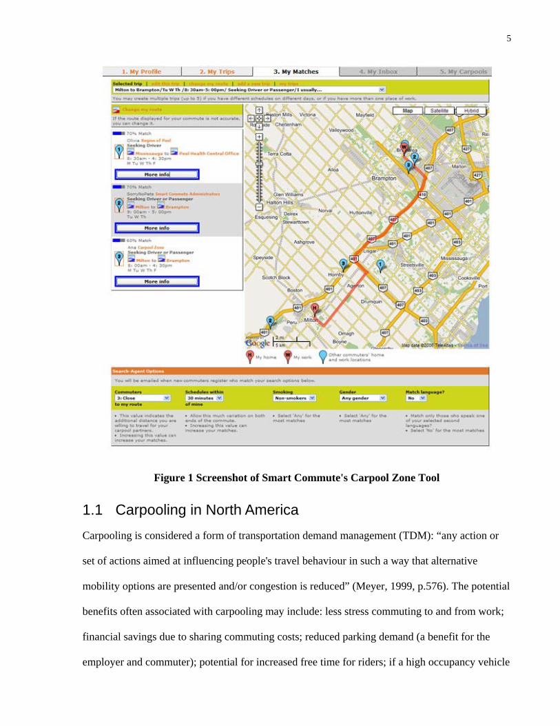
One of the key tools deployed in support of Smart Commute is the Carpool Zone, a free

online ride-matching service that matches commuters who live and work near each other and

travel at similar times (Figure 1). The purpose of this research is to investigate the carpooling

processes associated with Smart Commute users. The study has been designed to advance current

thinking about the factors that explain why some users are more capable of forming and starting

to carpool than others. Prior research on the understanding of the carpooling process within the

GTHA suggests that geographical proximity to other users, workplace TDM policies, the

scheduling of work, and commuter role preference influence carpool formation (Buliung et al.,

2010). This thesis, however, is concerned with extending this understanding by determining

whether firm characteristics and the built environment play an important role in this process and

if so, how. With respect to the geography of carpooling, the thesis extends prior work by

attempting to identify and then control for the presence of spatial effects that could undermine

the robustness of model results.

5

Figure 1 Screenshot of Smart Commute's Carpool Zone Tool

1.1 Carpooling in North America Carpooling is considered a form of transportation demand management (TDM): “any action or

set of actions aimed at influencing people's travel behaviour in such a way that alternative

mobility options are presented and/or congestion is reduced” (Meyer, 1999, p.576). The potential

benefits often associated with carpooling may include: less stress commuting to and from work;

financial savings due to sharing commuting costs; reduced parking demand (a benefit for the

employer and commuter); potential for increased free time for riders; if a high occupancy vehicle

6

(HOV) lane is available - trips may take less time; potential savings in auto-emissions due to

reduced vehicle use by all members of the carpool (Commuter Connections, 2011). However at

the same, carpooling has been criticized for several reasons, including: scheduling constraints;

the wide spatial extent of home, work, or study would reduce the prospect of finding good

matches; passengers of carpools don’t have access to a vehicle for personal trips during the day;

personality conflicts; people might simply have a negative experience carpooling (Black, 1995;

Morency, 2007).

The recent data on carpooling in North America indicate contradicting trends between

Canada and the United States. Carpooling mode share in Canada increased over time from 7.06%

in 2001 to 8.27% by 2006 (Statistics Canada, 2009). Conversely, the United States encountered a

decline in carpool propensity with only 12.19% in 2000 to 10.08% by 2004 (Pisarski, 2006).

Similarly, Ferguson (1997) reported a 32% decline in carpooling of all US work trips between

1980 and 1990 to just 13.4%.

1.2 Defining Carpooling A broad definition of carpooling can be “anyone who shares transportation to work in a private

vehicle with another worker” (Teal, 1987, p.206). Similarly, ridesharing has been described as

the situation “when two or more trips are executed simultaneously, in a single vehicle”

(Morency, 2007). In the literature, the two terms are often used interchangeably to emphasize the

sharing of a vehicle for travel. The conceptualization of carpooling seems to vary across the

literature. In one perspective, carpooling can be disaggregated into three categories (Teal, 1987):

1) Household carpoolers (commutes with at least one other work from the same household)

2) External carpooler (who shares driving responsibilities with unrelated individuals)

7

3) Carpool riders (who commutes with other unrelated workers but ride only and never provide a

vehicle).

Similarly, Levin (1982) defined carpooling by thinking about a preferred driving

arrangement as “a choice between serving as a driver, serving as a rider, or sharing driving

responsibility with others” (Levin, 1982, p.72). Carpools can be formed internally (i.e., family

members in the same household) or externally (i.e., friends or acquaintances). Morency (2007)

looked at household arrangements, producing the term intra-households ridesharing (IHHR) as

car passengers and car drivers belonging to the same household. Her study revealed that

approximately 70% of all trips made by car passengers in the Greater Montreal Area were the

result of IHHR.

Carpooling also, and perhaps surprisingly, exists as a legislative construct. For example,

the legal definition of carpooling, as per the Public Vehicles Act of the Province of Ontario, is as

follows:

“In this Act,

“Board” means the Ontario Highway Transportation Board; (“Commission”)

“bus” means a bus as defined in the Highway Traffic Act; (“autobus”),

(a) with a seating capacity of not more than 10 persons,

(b) while it is transporting not more than 10 persons including the driver on a one-way or round

trip where the taking of passengers is incidental to the driver’s purpose for the trip.

“a trip” described in (b) includes a round trip between the residences, or places reasonably

convenient to the residences, of any or all the driver and passengers and a common destination,

8

including the driver’s and passengers’ place of employment or education, or a place reasonably

convenient to the driver’s and passengers’ various places of employment or education.

(c) no fee is charged or paid to the driver, owner or lessee of the motor vehicle for the

passengers’ transportation, except an amount to reimburse the expenses of operating the motor

vehicle

(d) driver does not take passengers on more than one one-way or round trip in a day.

(e) the owner of the motor vehicle, or the lessee of the motor vehicle if it is leased, does not own

or lease more than one motor vehicle used as described in (a,b) unless the owner or lessee is the

employer of a majority of the persons transported in the motor vehicles.

(f) a motor vehicle described in (a,b) does not include a motor vehicle while being operated by or

under contract with a school board or other authority in charge of a school for the transportation

of children to or from a school.

The most recent definition emerged following back and forth legal disputes regarding

competition for shared rides. The issues were resolved on April 2009 when amendments were

conceived in Bill 118 (Countering Distracted Driving and Promoting Green Transportation Act)

to allow more flexibility for carpool formation and usage in the Province. Prior to the

amendment, it was illegal to carpool or rideshare in Ontario with someone unless all of the

following criteria were met (PickupPal, 2009):

• You must travel from home to work only (no rides to schools, hospitals, food banks,

etc.)

9

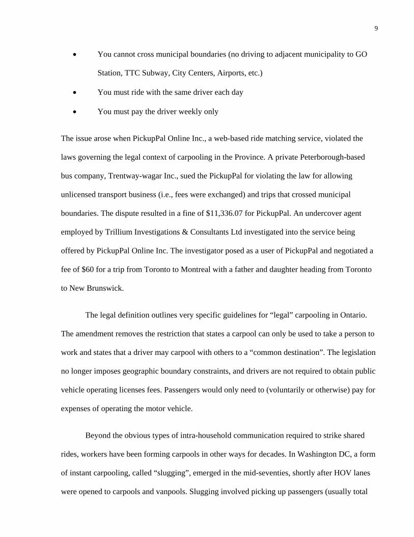
• You cannot cross municipal boundaries (no driving to adjacent municipality to GO

Station, TTC Subway, City Centers, Airports, etc.)

• You must ride with the same driver each day

• You must pay the driver weekly only

The issue arose when PickupPal Online Inc., a web-based ride matching service, violated the

laws governing the legal context of carpooling in the Province. A private Peterborough-based

bus company, Trentway-wagar Inc., sued the PickupPal for violating the law for allowing

unlicensed transport business (i.e., fees were exchanged) and trips that crossed municipal

boundaries. The dispute resulted in a fine of $11,336.07 for PickupPal. An undercover agent

employed by Trillium Investigations & Consultants Ltd investigated into the service being

offered by PickupPal Online Inc. The investigator posed as a user of PickupPal and negotiated a

fee of $60 for a trip from Toronto to Montreal with a father and daughter heading from Toronto

to New Brunswick.

The legal definition outlines very specific guidelines for “legal” carpooling in Ontario.

The amendment removes the restriction that states a carpool can only be used to take a person to

work and states that a driver may carpool with others to a “common destination”. The legislation

no longer imposes geographic boundary constraints, and drivers are not required to obtain public

vehicle operating licenses fees. Passengers would only need to (voluntarily or otherwise) pay for

expenses of operating the motor vehicle.

Beyond the obvious types of intra-household communication required to strike shared

rides, workers have been forming carpools in other ways for decades. In Washington DC, a form

of instant carpooling, called “slugging”, emerged in the mid-seventies, shortly after HOV lanes

were opened to carpools and vanpools. Slugging involved picking up passengers (usually total

10

strangers) along a designated "slug line" so that drivers would have enough additional passengers

to meet the required three-person HOV-lane requirement (Slug-Lines.com, 2009). The rationale

for engaging in slugging is that it would save time for both parties travelling to the same

destination. The traffic in Washington DC during rush hour is known to be the fourth worst in

the United States (INRIX, 2010).

More recently, the potential of using information and communications technology (ICT)

to form carpools has been enhanced by the availability of smart phones and 3G networks. There

are several examples of web-based ride matching tools available for either one-time or long term

usage (e.g., Pickup Pal, eRideshare.com, Carpool World, Zimride, Carpool Zone). Recently,

these tools have been integrated with social networking applications (i.e., Facebook and Twitter)

with a view to facilitating the carpool matching process. Moreover, PickupPal has released a free

iPhone app of their tool for tech-savvy users to use their iPhone's GPS functionality to identify

start/end locations and correspond with other users for easier matching.

1.3 History of Carpooling The history of carpooling can be described as a series of waves, interest in the mode seemed to

peak in times of crisis, and then abate during recovery. Carpooling first appeared in the United

States during World War II (early forties) due to oil and rubber shortages (Japan seized

plantations in the Dutch East Indies that accounted for 90% of the U.S. rubber supply)

(HowToStartACarpool.com, 2011). Using a propaganda campaign, the US government

encouraged carpooling to help conserve oil for use in military operations. A poster from 1943 by

Weimer Pursell persuaded the public to carpool by suggesting "when you ride ALONE you ride

with Hitler!". Following WWII, gas prices became more affordable and the surge of single-

occupant vehicle (SOV) ownership and use became increasingly evident.

11

Later, the Organization of Petroleum Exporting Countries (OPEC) oil crisis in 1973, a

petroleum shipping embargo on nations (i.e., United States, Western Europe) supporting Israel

during the Yom Kippur war with Syria and Egypt, produced another wave of interest. Failure to

resolve the conflict quickly and the resulting shortage of supply, resulted in extremely high gas

prices and even cases where the pumps simply ran dry. During this bleak period, a short-term

increase of 21.4% in carpooling was observed in the United States from 1970 to 1980 (Ferguson,

1997). Furthermore, the 1979 energy crisis in the US increased carpool propensity due to the

wake of the Iranian Revolution. During this time oil prices were pushed up, the US reduced their

dependency on foreign oil and encouraged citizens to switch to sustainable transport alternatives

(Brunso and Hartgen, 1981). Following the early 1980s, a decline in carpooling was observed, a

decline that seemed to slow somewhat by the late 1990s. In 1970, the share of carpoolers among

American commuters was approximately 20.5%. By the year 2000, this value substantially

decreased to 11% (Ferguson, 1997). According to the Census Bureau's American Community

Survey, the mode share of carpoolers in the United States is approximately 10.08% by 2004.

Carpooling was relatively stable in the seventies and even the early eighties. The most

significant decline in carpooling occurred in the mod-eighties but slowed down in the late

nineties. Ferguson (1997) generated a logit model of mode choice from the Nationwide Personal

Transportation Survey (NPTS) to explain the decline in carpooling. The author identified four

major sources for decline that occurred between 1970 and the early 1990s:

1) The single largest source of recent decline in carpooling was attributed to auto availability. It

appears that the average number of vehicles per household increased from 1970 to 1990. This

accounted for 38% of the overall declined observed.

12

2) The second source was suggested to be from falling marginal motor fuel cost which attributed

to 34% decline in carpool overall between 1970 and 1990.

3) The third source is attributed to age and education. The attainment of a high school diploma

rose from 44.6% in 1970 to 75.2% in 1990 for people aged 25 and older. The mean age of US

resident also increased from 28.1 years in 1970 to 33.0 years in 1990. These changes had an

impact of 24% decline in carpools.

4) Lastly, the fourth largest source of the recent decline (9%) in carpooling is related to gender

and lifestyle. Female labour force participation increased from 41.4% in 1970 to 56.8% in 1990,

work related travel demand increased with the influx of new workers to the economy.

The resurgence of carpooling in recent years is evident from our current unstable

economy and fluctuating fuel prices. Carpooling is beginning receive some favour as an

alternative option for many commuters. The proportion of SOV use among workers has

decreased in Ontario, from 72.6% of workers in 2001 to 71.0% in 2006. In contrast, the

proportion of workers in Ontario riding as passengers increased from 7.1% in 2001 to 8.3% in

2006 (Statistics Canada, 2009). The rise and combination of old and new technologies such as

information communication technologies (e.g., computers, mobile phones, hand held devices,

Internet), geographic information systems (GIS) and global positioning systems (GPS) has eased

the formation of carpools amongst potential users by increased mobility and access to resources.

The use of ICT to promote carpooling has also been shown to be “effective as traditional ride-

matching and may reach a user population different than that of the traditional ride match

system” (Dailey and Meyers, 1999, p.31).

13

1.4 Research Objectives The aim of this research is to advance our understanding of the carpool formation and use

process in the GTHA. The study addresses the following research objectives:

(1) to study the role of the built environment on carpool formation in the GTHA;

(2) to examine the differences and similarities between Carpool Zone users whom have formed

and not formed carpools;

(3) to uncover the influence of the spatial distribution of observations (i.e., spatial

autocorrelation) on the model results;

(4) to improve regression modeling by considering and controlling for spatial effects (i.e., spatial

autocorrelation).

1.5 Outline of Thesis The thesis is divided down into six separate chapters. Chapter 1, the introduction has been used

to define carpooling, refer to the history of the practice, and to present the past and contemporary

state of carpool US primarily in North America. The literature review in Chapter 2 provides an

extensive introduction to and summary of findings from carpool research, attention is uniquely

given to what is or is not know about the role of the built environment in carpool formation.

Chapter 3 presents the study area, discusses the data, and outlines the research methods. Chapter

4 provides descriptive analysis of the Smart Commute sample, results from logistic regression

modelling, and findings from spatial modelling. A discussion of the results follows in Chapter 5.

The last section, Chapter 6, summarizes the findings, provides policy recommendations, and

discusses the potential for future research.

14

2 Literature Review The main objective of the thesis is to advance the state of knowledge about carpool formation

and use. While several determinants of carpooling have been reported in the literature, less is

known about how the built environment relates to carpool formation. The built environment

refers to the man-made surroundings that human activities occur and can be described in terms of

density, diversity, and design (Cervero and Kockelman, 1997). It is potentially important to

examine the effect of the built environment on carpooling because previous studies have

demonstrated associations between trip outcomes (i.e., trip frequency, trip length, mode choice,

and vehicle miles travelled) and the built environment (Ewing and Cervero, 2001). It is important

to note that much of the carpooling literature has been developed for the urban areas of the

United States (Teal, 1987; Ferguson, 1997; Canning et. al, 2010). The findings from these

studies should not be considered directly comparable to work conducted in Canada (Buliung et

al., 2010) due to differences in demographics, spatial economy, built environment and urban

growth policies. However, these studies offer important findings on carpool formation and use in

urban environments.

This chapter reviews the literature on carpooling and is divided into the following

subsections: socio-economic and demographic characteristics (2.1), motivation for carpooling

(2.2), workplace characteristics (2.3), household auto-mobility (2.4), commute distance (2.5),

scheduling of work (2.6), role preference (2.7), transportation demand management (2.8), and the

built environment (2.9). Section 2.10 summarizes the key findings from the literature review and

identifies the gaps in the literature that the research will attempt to answer.

15

2.1 Socio-economic & Demographic Characteristics The literature presents conflicting findings with respect to the role of socio-demographic

characteristics on carpooling and carpool formation. Several studies have found little to no

correlation between socio-demographic characteristics and carpooling (Canning et. al, 2010;

Benkler, 2004; Kaufman, 2002; Teal, 1987; Horowitz and Sheth, 1978; Ferguson, 1997). These

studies often examine socio-demographic characteristics alongside more salient factors. For

example, Buliung et al. (2010), suggest that geographical proximity to other users; workplace

TDM policies; the scheduling of work; and commuter role preference increased the odds of

successfully forming carpools more than socio-demographic characteristics. Other studies have

reported links, particularly between gender, age, income, ethnicity, education and household

composition, and carpooling (Teal, 1987; Camstra, 1996; Tischer and Dobson, 1979; Kaufman,

2002; Ferguson, 1995).

In terms of gender differences, the findings in the literature on carpooling propensity

between males and females are conflicting. Various studies have suggested that females tend to

be more successful in the carpool formation process than males (Koppelman et al.,1993;

Brownstone and Golob, 1992). Other studies, however, suggests that men, who have higher

wages than females, would more likely have access to a private automobile (Blumenberg &

Smart, 2010). Many studies looked at "trip chaining", or making short trips to/from work, and

found that shopping and errand related stops are significantly higher for females than males

(McGuckin and Nakamoto, 2005; Strathman et al., 1994; Al-Kazily et al., 1994). Reasons that

may explain this include: dropping a child off, shopping for groceries, and other family

responsibilities. Concas and Winters (2010) determined that those who carpooled had a reduced

16

opportunity to engage in trip-chaining activities. With respect to trip-chaining, females are trip-

chaining more to than males to fulfil household obligations, and thus less likely to carpool.

With respect to age, studies have generally shown that younger people tend to be more

successful in forming carpools than older people (Baldassare, 1998; Charles & Kline, 2006;

Jakobsson et al., 2000). One explanation, that has received little attention, is that younger people

may have greater accessibility and comprehension of information and communications

technologies (i.e., smart phones and the Internet) that could be used to more readily enable

carpooling than other legacy technologies. Correia & Viegas (2011) found this to be the case,

particularly for carpooling within the university context. In contrast, the literature has also

suggested that older people are more likely to succeed in forming carpools (Tischer, 1979).

The literature on household composition consistently reports that individuals living in a

large household have a greater chance to form carpools (Tischer, 1979; Brownstone, 1992;

Charles, 2006; Brunso et al., 1979, Blumenberg and Smart, 2010). In the Greater Montreal Area,

a study found intra-household ridesharing (IHHR) accounted for approximately 70% of all trips

made by car passengers (Morency, 2007). In addition, Collura (1994) reported that of those who

carpooled, the majority (60%) did so with family members.

A few studies have shown a relationship between ethnicity/immigration and carpool

formation. Charles and Kline (2006) examined whether social capital engages people of the same

race to share in common activities such as carpooling. The report found that Hispanics carpooled

the most, four times as much as whites. Similarly, Cline et al. (2009) found that Hispanic

immigrants were 1.4 times more likely to carpool than non-Hispanic whites.

17

This research will consider how socio-economic and demographic characteristics

influence carpool formation relative to several other non personal factors. For example, a

previous study on employer-led carpool schemes found that motivational factors (e.g. cost

savings, environmental concern) bear greater influences in carpool formation than demographic

characteristics (Canning et al., 2010).

2.2 Motivation for Carpooling Carpooling has been shown to associate with motivational issues factors, perhaps more so than

other things. The motivation issue spans both attempts by exogenous organizations to motivate

workers to carpool (e.g., world war two propaganda campaigns), and intra-personal

considerations, that may or may not materialize as a result of an individual’s experiences. Cost-

saving is a major motivational factor that has been discussed frequently throughout the literature.

It is generally accepted that people with lower incomes are more inclined to use alternative

modes of transportation such as transit and carpooling, largely because the automobile may be an

unaffordable option (Baldassare et al., 1998; Hwang & Giuliano, 1990; Correia, 2011). Canning

et al. (2010), found that ‘saving money’, related to commuting costs, appears as a very important

or quite important concern for most.

The affordability of a private vehicle is related to educational attainment and income

generation. The median net worth (in 2005) for households with at least one member possessing

a university degree is $237,400. The median net worth (in 2005) for households with just a high

school diploma is substantially less at $120,007 (Statistics Canada, 2008c). Studies have found

people with lower educational attainment engage in carpools more often due to their inability to

obtain higher paying jobs, the lack of income is a barrier to entry into the automobile market

(Ferguson, 1997; Baldassare, 1998).

18

Concern for the environment is another major motivational factor affecting the decision

to carpool. Canning et al. (2010) reported ‘environmental concern’ rated either very important or

quite important by a majority (79.8%) of respondents. Jacobson and King (2009) suggest that the

effect of adding one additional passenger to every 100 vehicles would lead to an annual savings

of 0.80-0.82 billion gallons of gasoline. Other studies have also identified environmental

awareness as a motivation to carpool (Collura, 1994; Benkler, 2004). Of course, it is difficult to

disentangle the links between environmental and economic concerns, fuel savings produces

benefits to both domains.

2.3 Workplace Characteristics Workplace characteristics such as employment composition and firm size have shown to either

advance or inhibit carpool formation. The general consensus is that large single-tenant worksites

generally increase the chances of carpool formation and use (Cervero and Griesenbeck, 1988;

Ferguson, 1990; Brownstone and Golob, 1992; Teal, 1987). A larger firm, in either the service or

manufacturing sectors could produce greater opportunity for people to be matched. There is

some data suggesting that economic sector matters. People employed in nonprofessional jobs

(i.e., requiring less intellectual skills) have been shown to be more likely to initiate carpooling

because of cost-saving concerns (Cervero and Griesenbeck, 1988). Similarly, Cline et al (2009),

found those employed in construction, extractive industries, and farming are more likely to

engage in ridesharing than those employed in other industries.

2.4 Household Auto-Mobility Household auto-mobility (i.e., access to a car) also appears to associate with carpooling.

Ferguson (1997) reported that the average number of persons per household fell from 3.16 in

1969 to 2.56 in 1990, while the average number of vehicles per household increased from 1.16 to

19

1.77 during the same time period. These figures accounted for 38% of the overall observed

decline in American carpools. Living in a household with fewer vehicles than workers can

advance carpooling as much as 2.6 times (Cline et al., 2009). Similarly, Teal (1987) revealed

relatively low rates of carpooling within households with high vehicle to worker ratios. Other

research has shown that persons from households where the number of licensed drivers was

greater than the number of available vehicles had higher carpool propensities (Koppelman, 1993;

Correia and Viegas, 2011). Blumenberg and Smart (2010) found that increased auto availability

exhibits a strong negative association with non-SOV modes such as transit and carpooling.

However, when users were already enrolled in an employer-led carpool scheme, having no

regular access to their own vehicle was perceived as unimportant (Canning et al., 2010).

2.5 Commute Distance Carpooling is typically thought of as a longer distance alternative. The potential for ridesharing

is more likely to occur for longer commute distances because the time spent in picking up others

along the way would be relatively small compared to the total travel time. Cervero and

Griesenbeck (1988) examined the suburban commuting behaviour and travel patterns among

workers in Pleasanton, California. They found that successful carpools were associated with

long commute distances. Other factors included working for a large company at a single-tenant

site, and working in non-professional and non-management positions. Cervero and Griesenbeck

(1988) found that there was a 37% probability for a clerical employee to carpool if he/she had a

50 mile trip when compared to only 17% if he/she commuted 4 miles.

Research conducted by Lue and Colorni (2009) reported the opposite, but for a different

and highly specialized population, university students. The authors described two possible

different choices that students from the Politecnico di Milano University may take, related with

20

the destinations of carpool trips. In the first situation, called “direct”, they assumed that the

students would always want to carpool directly to campuses of Poltecnio. In the second situation,

called “park and ride”, they assumed that students, except all those living in municipalities close

to the university campuses, carpool to public transit stops where they can park and ride. The park

and ride scenario performed better than the direct scenario, mainly because of the shorter

distance to travel and, as a result, greater availability of matches, when compared with the direct

scenario. Carpoolers may prefer traveling shorter distances because of ease and comfort. Tischer

and Dobson (1978, p.143), found "perceptions of carpool schedule flexibility, cost, safety and a

short wait in traffic were the prime factors associated with potential carpool shifting".

Furthermore, Levin (1982) found that carpooling desirability decreased with increasing time to

pick up and deliver passengers.

2.6 Scheduling of Work A person’s work schedule is an important factor that dictates whether carpools can be formed

with other individuals. Cervero and Griesenbeck (1988) examined the effect that flex-time

programs at the workplace have on carpooling. Flex-time is a program that offers workers more

flexibility on their arrival and departure times (usually an hour deviation). This incentive would

help offset peak demands on roadways and alleviate traffic congestion. The study found that

workers that enrolled in the flex-time program and commuted at atypical times were more likely

to drive alone than carpool. Similarly, Tsao and Lin (1999) and Ferguson (1990), found the

temporal regularity of work was an important factor for carpool formation and usage. Habib and

Zaman (2011) found workers with compressed work week or flexible office hours were less

likely to consider carpooling as a viable commuting mode. Once considered, however, the final

choice of carpooling is positively influenced by the option of having a flexible work schedule.

21

2.7 Role Preference Preferred driving arrangement refers to the choice between serving as a driver, serving as a rider,

or sharing driving responsibility with others. Levin (1982) observed a greater preference for

shared driving arrangements due to the tradeoffs of the economic advantages of being the driver

and the perceived greater comfort and convenience of being a rider. In this research, the

relationship between the role of carpooling (i.e., drive only, ride only, and share) and the

likelihood to form and use successful carpools will be investigated.

2.8 Links with Transportation Demand Management (TDM) Transportation demand management (TMD) programs are implemented at the workplace to

increase the awareness of sustainability and to reduce single occupancy vehicle use (Koppelman

et al., 1993). Koppelman et al (1993) classifies transportation demand management into two

types of programmes: ridesharing incentives or SOV disincentives. Subsidy, SOV penalty, or

transport pricing in general may affect carpooling. Brownstone and Golob (1992, p.21), found

that “providing all workers with reserved parking, ridesharing subsidies, guaranteed rides home,

and high-occupancy vehicle lanes would reduce drive-alone commuting between 11 and 18

percent”. Guaranteed ride home (or Emergency ride home) program provides “commuters who

regularly vanpool, carpool, bike, walk, or take transit with a reliable ride home when one of life's

unexpected emergencies arises" in the form of "ride home by cab, rental car, bus or train

expenses" (Commuter Page, 2011). Several studies have found GRH as a reliable TDM policy to

encourage ridesharing in the workplace and would reduce SOV use (Polena and Glazer, 1991;

Correia and Viegas 2011; Brownstone and Golob, 1992).

Priority parking encourages ridesharing by proving parking spots closer to the workplace

(i.e., more desirable locations relative to the workplace) and is exclusively reserved for

22

carpoolers. Canning et al. (2010) found priority parking for carpoolers was considered important

to participants even when there is no significant parking pressure. This approach provided

incentives for workers to partake in sustainable options. Similarly, Baldassare et al. (1998)

established that suburban commuters in Orange County were more inclined to switch mode upon

cash incentives than penalties on automobile usage. In contrast, Washbrook et al. (2006)

observed whether road pricing can be a viable option to promote carpool propensity. It was

determined that the introduction of a $9.00 (CAD) road charge and $9.00 (CAD) parking charge

for workers in the Vancouver suburbs, would dramatically reduce the drive alone mode share to

17% and increase carpooling to 74% of the overall mode share. In addition, Jacobson and King

(2009) found that when parking fees and/or road tolls were imposed the attractiveness to switch

to carpooling became less desirable.

2.9 Built Environment The potential to influence travel behaviour (i.e., mode choice, trip frequency, trip length,

vehicles miles traveled) by altering the built environment is an extensively studied topic in urban

planning. Ewing and Cervero (2010), in their extensive review on the subject, found over 200

articles published within this research domain. One of the important goals today for

transportation planners is to understand how to design neighbourhoods and large cities with the

intent to reduce automobile dependency, environmental concerns, and traffic congestion. The

three principal dimensions of the built environment (i.e., density, diversity, and design)

conceived by Cervero and Kockelman (1997) are thought to influence travel demand. In recent

studies, destination accessibility and distance to transit were also included as additional

dimensions affecting travel behaviour (Ewing & Cervero, 2001; Ewing et al., 2009). Cervero and

Murakami (2009), revealed that higher population densities in 370 US urbanized areas are

23

strongly associated with reduced vehicles miles traveled (VMT). It is hypothesized that in places

with high densities, there will be less likelihood for carpool formation because other mode of

transport may be more dominant (e.g., walking, cycling, and public transit). Previous studies

have suggested that employees who work in diverse/mixed-use commercial areas are more likely

to commute by alternative modes such as transit, cycling, or walking (Kuzmyak et al., 2003;

Modarres, 1993). As a result, it is hypothesized that users working in diverse land-use area

would less likely carpool because of the availability of other mode choices. With respect to street

design, a connected road network (i.e., grid network) is known to provide better accessibility

than hierarchical road networks (Handy, Paterson and Butler, 2004). It is hypothesized that users

would have greater success in carpool formation in areas with well connected road networks

because of the ease of the accessibility with other users. With respect to the carpooling

literature, little research has been conducted to explain the association between carpool

propensity and the built environment. This study will investigate how the various dimensions of

the built environment influence the carpooling decision.

2.10 Summary & Synthesis This brief literature review offers insight into the carpool formation process. The literature

presents contradicting results with respect to socio-demographic characteristics and carpool

formation. At one end, studies have found little or no correlation between socio-demographic

characteristics (age, income, and gender) and carpooling because other factors (e.g., workplace

characteristics) emerge as more important when modeled together. However, socio-demographic

characteristics are also seen as important determinants for carpooling. For example, several

studies have found females more successful in forming carpools due to auto mobility access and

having more family responsibilities. This research will assess whether socio-demographic

24

characteristics are important determinants for carpooling. Cost-savings and environmental

concerns are among the most important motivators reported in the literature that explain why

people carpool. This study will also examine whether these key motivators are important in the

case of Carpool Zone users employed in the service-producing industries.

With respect to workplace characteristics, large single-tenant firms have been shown to

encourage carpooling due to the large potential for ride matching. The services-producing

industries hold the largest share of workers in the workforce and their growth rate is continuing

to increase. For example, between 2001 and 2009, the goods-producing industries decreased at a

rate of 0.3%, while the services-producing industries showed an increase in GDP of 2.4% per

year (Industry Statistics, 2009). It is expected that most carpoolers would belong in this group.

However, the literature has also stated that people employed in nonprofessional jobs were more

likely to form carpools because of cost-saving concerns. The literature is consistent with its

findings on household auto-mobility and carpool formation. Generally, when there are more

adult workers in the household than household automobiles, carpooling propensity increased.

Differences in commute distances have been reported in the literature. Long commute distance is

positively associated with carpool formation due to the time spent picking up others along the

way would be relatively small compared to the total travel time. In contrast, longer commute

distance have also worked against carpooling as it decreased ease and comfort for its users.

Other TDM initiatives can compete with or perhaps complement carpooling, if patronage

and individual commitment to the program is high. Flex-time programs offer workers more

flexibility on their arrival and departure times. In the literature, flex-time is characterized by

atypical work a schedule which is associated with decreased carpool propensity because of the

25

lack of available matches. TDM programs such as Emergency ride home (ERH) and priority

parking both appear to positively correlate with carpooling.

With respect to role preference, the study will investigate whether shared driving

responsibility carry more weight than users only willing to either drive or ride alone. In the

literature, users willing to share driving arrangements were the most successful.

With regard to this study, one of the major gaps discovered through the review is that

little is known about the relationship between carpooling and the built environment. This study

will investigate how the various dimensions of the built environment, conceived by Cervero and

Kockelman (1997), influence carpooling. These dimensions include: population density, land use

diversity, street design, destination accessibility, and distance to transit.

3 Study Area, Data, Methodology The main objective of this research is to study the relationship between the built environment

and carpool formation – a topic not well understood. The second goal of the work is to consider

how spatial effects might alter such relationships when they are described statistically through

logistic regression. The study design involves specification and estimation of logistic regression

models to explain the connection between the built environment and the decision to carpool. The

logistic regression approach has been used in carpooling studies before (Buliung et al., 2010;

Canning et al., 2010; Blumenber and Smart, 2010; Cline et al., 2009; Zaman and Habib, 2011).

The data set is derived from a combination of data sets provided from several sources: Carpool

Zone user profiles and trip data from Metrolinx, Carpool Zone user satisfaction survey results

from Metrolinx, 2006 census data from Statistics Canada, and GIS data (road and land use

layers) from DMTI Ltd. Logistic regression describes the relationship between a dichotomous

26

response variable (i.e., carpool status: formed vs. non-formed) and a set of explanatory variables

(i.e., built environment variables).

With regard to the second objective of the work, uncovering the influence of the spatial

distribution of observations (i.e., spatial autocorrelation) on the model results, statistical analyses

that does not control for spatial autocorrelation could produce biased parameter estimates and

increase the chance for type 1 errors (Dormann et al, 2007). The concept of spatial

autocorrelation stems from Tobler's First Law of Geography: "Everything is related to everything

else, but near things are more related than distant things" (Tobler, 1970, p.236). Classical

inferential statistical methods (e.g., regression analysis) assume that measured observations are

independent from one another. However, in spatial data, observations at proximal locations

could exhibit some similarities (i.e., spatial autocorrelation). In order to compensate for spatial

autocorrelation, an autologistic regression model can be specified, adding an extra explanatory

variable to capture the effect of neighbouring responses on individual cases (Augustin, 1996).

This chapter provides a description of the study area, data, and research methods. The

chapter introduces the study area (Section 3.1) and justifies its selection for the carpooling study.

Section 3.2.1 describes the systematic approach of data filtering to produce the final dataset for

regression and mapping analysis. In addition, the data limitation of the dataset is briefly

discussed. The methods section (Section 3.2) describes the model specification (Section 3.2.2),

mapping hotspots (Section 3.2.4.1), and the autologistic regression modeling approach (Section

3.2.4.2). The description of all explanatory variables in greater detail is outlined in Section 3.2.3.

3.1 Study Area Smart Commute, a transportation management association (TMA), provides TDM programs

throughout the Greater Toronto & Hamilton Area (GTHA) to both employers and individuals,

27

the core urbanized territory of the Greater Golden Horseshoe (GGH). The study area is the

GTHA - the urban core of the GGH. The spatial extent of Smart Commute TMA coverage

parallels the boundaries of the GTHA. The planning goal of the TMAs is to provide

transportation demand management (TDM) programs to alleviate traffic congestion and

encourage sustainable transportation (i.e., walking, cycling, and biking) to its users. As of July

2011, there were 12 TMA offices working with the region's municipalities, post-secondary

educational institutions, and private firms (Figure 2).

Figure 2 TMA of Smart Commute

The GGH is considered, “one of the fastest growing regions in North America” and

attracts many people for its “high quality of life and economic opportunities” (MPIR, 2006, p.6).

It is a dense urbanized region that wraps around the western end of Lake Ontario, with

28

boundaries stretching south to Lake Erie, north to Georgian Bay, east to Peterborough, and west

to Waterloo (Figure 3). The GGH contains 9 of the country’s 33 census metropolitan areas

(CMA) that represent 84% of Ontario’s population. It is home to 8.1 million people (in 2006)

and is expected to increase to 11.5 million by 2031 (Hemson, Consulting, Ltd., 2005). A

comprehensive growth plan for the GGH has been prepared with a view to implementing the

Government of Ontario's mandate for "building stronger, prosperous communities by better

managing growth in this region to 2031" (MPIR, 2006, p.6).

Figure 3 Golden Horseshoe (Outer) & Greater Toronto Hamilton Area (Inner)

Source: Hemson Consulting Ltd.

29

Between 2001 and 2006, the GGH experienced rapid population growth along the

periphery of the urban core (i.e., City of Toronto). According to Statistics Canada (2006), these

municipalities include: Milton (+71.4%), Barrie (+23.8%), Ajax (+22.3%), Aurora (+18.6%),

Halton Hills (+14.7%), Oakville (+14.4%), Newmarket (+12.9%), Caledon (+12.7%), Waterloo

(+12.6%), Clarington (+11.4%) and Mississauga (+9.1%) (Statistics Canada, 2006). In contrast,

Toronto only experienced a 0.9% growth during this period. The rapid population growth in the

outer suburbs clearly exceeds growth in Toronto, a process that is driven by perceptions of

affordability and the suburbanization of jobs (Harris, 2004).

The so-called "Quebec City-Windsor Corridor" refers to the most densely populated and

industrialized part of the country. The region extends from Quebec City in the east to Windsor,

Ontario in the west, spanning 1,150 kilometres (VIARail, 2009). Parts of the GGH are located

within the Quebec City-Windsor Corridor. The GGH is considered Canada's most important

economic hub as it contributes for more than 50% of Ontario's Gross Domestic Product (GDP)

(OECD, 2010). The region is connected by a series of major transportation routes, vital for the

movement of people and goods. A majority of the 400-series highways fall within the GGH

forming the province's main road transportation corridor. Of these highways, the King's Highway

401 is North America's busiest highway and daily traffic sometimes exceed 500,000 vehicles

according to average annual daily traffic counts (Federal Highway Administration, 2007). The

Ontario Chamber of Commerce estimates congestion to cost upwards of $5 billion in lost GDP

each year (Ontario Chamber of Commerce, 2004).

With regard to mode share in the GTHA, according to the 2006 Transportation

Tomorrow Survey, the primary choice of travel mode for work within the GTHA is auto driver

(63%), followed by auto passenger (16%), local transit (12%), walk & cycle (6%), other (2%),

30

and GO train (1%). The median trip length for an auto driver and auto passengers are 5.6 km and

4.1 km, respectively. In contrast, those who are commuting by the GO train are typically

travelling at a median distance of 30.2 km. The City of Toronto possesses the greatest share of

work trips in the GGH. In comparison to the GGH, Toronto has a higher local transit share

(27%), but still relatively high share of auto drivers (48%).

The policy environment aims to address the bias toward automobile use principally

through land use planning. The Growth Plan aims to build complete communities that are

characterized as "well-designed, offer transportation choices, accommodate people at all stages

of life and have the right mix of housing, a good range of jobs, and easy access to stores and

services to meet daily needs" (MPIR, 2006, 13). As a result, the Plan calls for compact urban

form or new urbanism development to achieve this goal. Compact urban form is characterized as

"a land-use pattern that encourages efficient use of land, walkable neighbourhoods, mixed land

uses (residential retail, workplace and institutional all within one neighbourhood), proximity to

transit and reduced need for infrastructure" (MPIR, 2006, p.41).

3.2 Methods

3.2.1 Dataset, Data Limitations, Data Filtering

The main data sources were acquired from Smart Commute (i.e., The Carpool Zone User

Satisfaction Survey, Profile Dataset, the Trip Dataset, and the Workplace Dataset) as secondary

data for the analysis. Secondary data is limited to the relevance of the research, availability of

data, and accuracy. These are individual level data, as such; ethics approval was acquired

through the University of Toronto: Office of Research Ethics. Individual description (profile

data), trips, and workplace information were linked using a unique ID given to each respondent.

Datasets

31

The advantage of using secondary data allows no additional investment in resources (i.e., time

and money) to collect the data and organize the dataset (Boslaugh, 2007, p.3). Personal

information (e.g., contact information) was stripped from the dataset for privacy and ethical

concerns. Data on factor not observed in the Metrolinx source, e.g., income, population, built

environment variables, were developed from other data sources (i.e., Canadian 2006 Census and

2007 DMTI Spatial CanMap Route Logistics) and spatially linked to each respondent. The

remainder of this section described each of the secondary datasets provided by Metrolinx.

Carpool Zone was launched in 2005, and by the end of 2007, the program had registered

4,774 users. Smart Commute conducted an electronic survey to evaluate the performance of

Carpool Zone and its participants in December 2007. The satisfaction survey used Likert scale

questions (i.e., responses ranging from poor to excellent) to uncover user's attitudinal

characteristics. Some of these questions included: rating of overall experience, ease of use,

privacy, ability to generate matches, and etc. Quantitative questions requested in the survey

included: age, commute time to work (min), and the number of household vehicles.

The satisfaction survey followed a cross-sectional approach: conducted to examine the

usage level of its users for only at one point in time (i.e., Winter 2007). The usage level forms

the response/dependent variable for the regression models. In the survey, users were asked to

indicate their usage level from nine options: 1) Having started carpooling with Carpool Zone

matches; 2) Waiting for carpool matches; 3) Waiting for better matches; 4) Waiting for a

response from a carpool suggestion sent; 5) Have formed a carpool, but we haven't started

carpooling yet; 6) Not applicable; 7) Other; 8) Have not yet entered trip information; 9) No

longer interested in carpooling. Users that responded to the first option were considered

"formed" carpoolers. Users that responded options 2-5 were labeled as "non-formed" users.

32

Carpool Zone users responding to options 6-9 were excluded from the analysis because or

incomplete or vague responses to discriminate between the two groups.

The full complement of 4,774 registered users was invited to participate in the User

Satisfaction Survey by e-mail. The exercise produced 1,422 responses, a 29.78% response rate.

Surveys were mailed electronically and users accessed them via a personalized link that enabled

individual identification of each user. The participation incentive was a draw for an iPod Touch

($375.00) and a $50.00 iTunes gift card. A reminder was sent 6 days prior to the end of the

survey, 319 responses following the reminder. Responses were linked respondent profile data,

data generated during user registration. Profile data include spatial identifiers (i.e., user's home

postal code), demographic data (e.g., age, income, language, number of household cars), driving

preference (smoke, commute method), and commute times.

A separate dataset containing user trip characteristics was also provided. These data

included: trip origin/destination, carpool role (i.e., drive/ride/share exclusively), scheduling and

programming (i.e., public or employer user). The dataset included 4,295 records/trips; however

several respondents had multiple entries. A set of criteria was developed to handle respondents

with multiple entries. The commute distances (obtained from the trip dataset) of multiple entries

were compared to select for the entry containing the mode (most frequently occurring) of trip

distances. The rationale for choosing the route with the ‘modal’ distance was that the respondent

would likely travel this particular route on a daily basis to/from work. When multiple entries

were unique, the longest trip was selected because it was consider the most likely trip from home

to work since chained trips (i.e., coffee trips) are typically much shorter in distance. Filtering of

trips and matching of the trip data to the individual data from the profile and user satisfaction

survey produced a sample of n = 613 cases.

33

The association between firm characteristics and the decision to carpool was also

examined in this study. Smart Commute provided data on workplace characteristics of each

respondent and contained 1727 records. The majority of respondents are employed within the

Mississauga (482) Smart Commute TMA region, followed by North Toronto & Vaughan (353),

and Brampton & Caledon (226). For each respondent, the dataset contained information on the

type of firm, firm size, number of carpool spaces, and the type of TDM strategies in place

including: emergency ride home (ERH), and/or flex time. Previous work has established the

importance of workplace characteristics, such as priority parking spaces, in employer-led carpool

schemes (Canning et al., 2010). It is therefore important to control for workplace transport policy

when studying carpool formation. Firm type was classified using the North American Industrial

Classification Standard (NAICS), to associate cases with participation in either the goods-

producing and services-producing industries (Table 1). As demonstrated through the literature

review, there is some indication that carpooling propensity varies by economic sector.

Goods-producing industries

Services-producing Industries

Manufacturing Information and Cultural Industries

Utilities Finance and Insurance

Public Administration

Health Care and Social Assistance

Educational Services

Other Services

Professional, scientific and technical services

Unknown (property manager group)

Table 1 Goods-Producing versus Services-Producing Industries

The primary goal of this study is to understand the effect of the built environment having on

carpool formation within the GTHA. The lack of research in this area is the underlying reason

34

why this study was carried out. The built environment dataset was compiled solely by the

researcher because data on the built environment was not available in the datasets provided by

Metrolinx. Using the trip origin and destination locations obtained from the trip dataset and the

2007 DMTI Spatial CanMap Route Logistics product suite, the following built environment

variables were created for the regression analysis: population density, Herfindahl-Hirschman

Index (a measure of diversity), street density, cumulative opportunities, and network distance to

nearest transit stop. The geographic scale chosen for the built environment variables was at the

dissemination level because it represented the smallest spatial unit available and data loss

because of spatial resolution would be at a minimum. The creation of built environment variables

in the dataset followed the three principal dimensions of the built environment (i.e., density,

diversity, and design) conceived by Cervero and Kockelman (1997). These dimensions were

expanded to also include destination accessibility and distance to transit that affected travel

behaviour (Ewing & Cevero, 2001; Ewing et al., 2009). These variables are discussed in further

detail in the subsequent subsection.

After joining various datasets (Satisfaction Survey & Profile Dataset, Trip Dataset,

Workplace Dataset, and the Built Environment Dataset) and undergoing several data filtering

processes, the sample size of the final dataset reduced from the original 1,422 sample to 358

respondents. The data filtering process was quite complicated and is illustrated further by Figure

4 (flowchart). The first dataset (Satisfaction & Profile data) provided each user's: demographics,

spatial factors, motivation for carpooling, and household auto-mobility. When the trip dataset

was added, the following attributes were added to each case: scheduling of work, firm transport

policy, role preference, commute distance, and commute pattern. Subsequently, the workplace

data added: firm type, firm size, number of carpool spaces at the firm, ERH program, and flex-

time. The last dataset, the built environment data, was created using data from the 2007 DMTI

35

Spatial CanMap Route Logistics product suite producing origin and destination measures of

population density, land use diversity (Herfindahl-Hirschman Index), street density, cumulative

opportunities, and network distance to nearest transit stop.

The study follows a cross-sectional approach, using secondary data, and was designed to study

carpool formation (formed vs. non-formed) of individuals at a particular point in time. The

primary advantage of using secondary data to conduct research is economy: the data has been

already collected by another individual/group, so the researcher does not need to devote

resources (e.g., time and money) in this stage of research. However, when using secondary data,

the researcher is only limited to the data collected by the other party. For example, the limited

types of data in the profile, satisfaction, trip and workplace datasets made it difficult to fully

grasp whether socio-demographic, motivational, spatial, and workplace characteristics had an

effect on carpool formation in the GTHA. Many of the variables generated in the final dataset

were derived from other sources (i.e., Canadian Census, DMTI Ltd.) to act as proxy for missing

data. For example, household income was acquired from the 2006 Canadian Census from users'

trip origin (home location) at the dissemination area (DA) scale. In doing so, concern for

ecological fallacy arises when the researcher makes an inference about an individual based on

aggregate data. The readers should be aware that aggregate statistics (from the DA-level)

describe group characteristics and do not necessarily apply to individuals within that group. In

addition, the researcher did not have input in the types of questions asked in the survey.

Data limitations

Another major drawback with the data was maintaining a consistent dataset throughout

the data filtering process. The various datasets acquired from Smart Commute had to be joined

via a unique user ID. The main concern arises from the trip dataset where multiple trips were

36

made for each unique user (i.e., chained trips) and choosing the best commute distance to

represent the user's commute to work. Another problem with consistency is that various datasets

(i.e., profile, satisfaction, trip, workplace) were given to the researcher at different time periods.

For example, workplace data from the Toronto-Central TMA could not be joined with the profile

and satisfaction datasets because the Toronto-Central TMA did not exist yet when the profile and

satisfaction surveys were generated. As a result, it was difficult to match users with incomplete

data in one of the datasets.

The 1,422 responses collected from the Carpool Zone Satisfaction Survey included several

responses that were either incomplete or unsuitable for the carpooling study. Two criteria were

implemented to narrow down to a sample of 1,009 respondents for the carpooling study:

Data Filtering

1) The respondent’s postal code (home/origin) had to be located within the study area (i.e.,

GTHA). Several respondents reported inaccurate postal codes posing problems for

mapping.

2) The respondent had to have answered the question on carpool usage level. Their response

on that question was necessary to construct the dependent variable.

Prior research has shown respondents participating in employer programs were twice as

likely (on average) than public users, to produce an operational carpool (Buliung et al., 2010).

Within the context of the Metrolinx Carpool Zone program, employer-based respondents have a

greater incentive to carpool than public users because of the benefits associated to the program

(i.e., ERH, flex time, prizes from draws, priority parking, and etc.). The researcher chose to only

examine the employer-based users of Carpool Zone and excluded public users from the sample

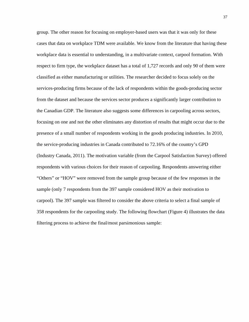
37

group. The other reason for focusing on employer-based users was that it was only for these

cases that data on workplace TDM were available. We know from the literature that having these

workplace data is essential to understanding, in a multivariate context, carpool formation. With

respect to firm type, the workplace dataset has a total of 1,727 records and only 90 of them were

classified as either manufacturing or utilities. The researcher decided to focus solely on the

services-producing firms because of the lack of respondents within the goods-producing sector

from the dataset and because the services sector produces a significantly larger contribution to

the Canadian GDP. The literature also suggests some differences in carpooling across sectors,

focusing on one and not the other eliminates any distortion of results that might occur due to the

presence of a small number of respondents working in the goods producing industries. In 2010,

the service-producing industries in Canada contributed to 72.16% of the country’s GPD

(Industry Canada, 2011). The motivation variable (from the Carpool Satisfaction Survey) offered

respondents with various choices for their reason of carpooling. Respondents answering either

“Others” or “HOV” were removed from the sample group because of the few responses in the

sample (only 7 respondents from the 397 sample considered HOV as their motivation to

carpool). The 397 sample was filtered to consider the above criteria to select a final sample of

358 respondents for the carpooling study. The following flowchart (Figure 4) illustrates the data

filtering process to achieve the final/most parsimonious sample:

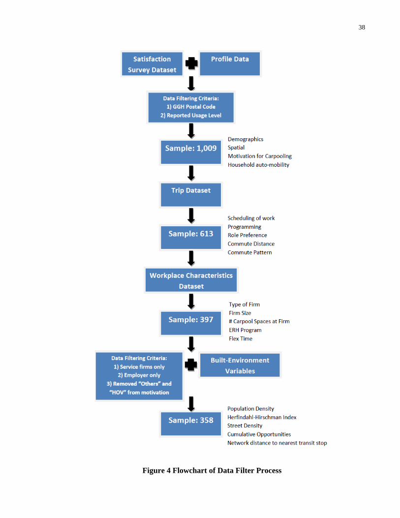
38

Figure 4 Flowchart of Data Filter Process

39

3.2.2 Model Specification

Model specification involves deciding the type of model (i.e., function) and what variables

are appropriate for analysis. Logistic regression is used here due to the presence of a discrete

outcome (carpool usage: formed or non-formed). Buliung et al. (2010) demonstrated the value of

applying logistic regression to the modeling of a carpool formation process. In this study, a

binary response variable was constructed from the satisfaction survey that asked for the

respondents’ usage level of Carpool Zone. Each respondent was classified into one of two

groups: 1) formed (coded as “1”) or 2) non-formed (coded as “0”). A formed respondent is

defined as a user having formed and started carpooling, at the time of survey, before other users.

In contrast, respondents in the following categories are classified as having not formed a carpool

at the time of survey: waiting for a match, waiting for better match, waiting on response, or

formed without starting.

The logistic regression model used in the study assumed the form:

∑=

+=

−

=n

iii X

1p1ploglogit(p) βα

where p is the probability of having started carpooling at the time of the survey, log(p/1-p) is the

log odds of forming a carpool, α is a regression constant, and βi is a coefficient to be estimated

for each explanatory variable xi

When a logistic regression model (binomial, or multinomial) is estimated with too many

variables, relative to the number of cases in the smallest category for the response, the regression

coefficients can be biased in both the positive and negative directions. This can influence the

validity of the model, yielding extreme values for the maximum likelihood estimates (Peduzzi et

. The logistic regression model generates the natural log of the

odds of successfully forming and using a carpool.

40

al., 1996). The number of events per variable (EPV) is the ratio of the number of cases in the

category of the dependent variable with the smallest number of cases to the number of variables.

Peduzzi et al. (1996) determined a minimum of 10 events per independent variable is

recommended to avoid biased regression coefficients. For this particular study, with 121 cases

(successes), only 12 independent variables, at the maximum, can be used in the logistic

regression model. While there is seemingly unlimited opportunity to over specify a model of

the sort used in this study, the number of available cases limits the analysis, and so a rather

parsimonious approach has been taken as the underlying philosophy for model specification.

The next step in model specification is to select the independent variables for the model. A two-

step approach to select the variables for this study was developed:

1) A set of bivariate logistic regressions was estimated, pairing each explanatory

(independent) variable with the response variable (carpool usage). To filter the first round

of independent variables, only those variables holding statistical significance at p ≤ 0.05

(95% confidence interval) were included in the next stage of filtering. It was assumed

that statistically significant variables from these unadjusted models will retain some

relevance in the multivariate specification.

2) Multi-colinearity (the independent variables correlating with one another) across the

explanatory variables that were significant from the bivariate regressions was also

examined. Pearson chi-square tests were conducted to examine the correlation amongst

the categorical variables, and the Pearson product-moment correlation coefficient is used

to identify correlation amongst the continuous variables. The presence of multi-

colinearity can introduce biases into regression models and produce large standard errors

for the related independent variables.

41

3.2.3 The Explanatory Variables Overview

This section describes all the explanatory variables modeled in the study (Table 2), explaining

how and why each independent variable was created.

Table 2 Variable Descriptions

Variable Name Description

(1) Demographics

Gender Female or male (reference category)

Age Age in years

Median household income Median household income in dissemination area

(DA-level) of residence.

(2) Spatial

Proximity to nearest carpool lot Network distance to closest government managed

carpool lot. These lots were typically located at

highway interchanges (metres).

Proximity to nearest Carpool Zone

User

Cumulative opportunities measure of Carpool Zone

users at varying buffer distances (metres).

(3) Motivation for Carpooling

Environment Concern for environment (reference category)

Don’t drive, or don’t have

access to a car

Level of personal auto-mobility

Cost savings Units unspecified in survey

Use of HOV lanes Use of high occupancy vehicle lanes, value of time

Other Other unspecified motivations

(4) Household Auto-mobility

Number of household automobiles Number of automobiles in the household

42

(5) Scheduling of Work

Typical vs. atypical schedule Typical work hours (Monday to Friday, between 8-

9 a.m. and 4 p.m.-5 p.m. Atypical work hours

(reference category, with a work schedule

deviating from above).

(6) Role Preference

Drive only Prefers to drive all of the time

Ride only Prefers to be a passenger all of the time

Share Prefers to share (reference category) driving

responsibilities, sometimes driving, sometimes a

passenger.

(7) Commute Distance

Network distance (km) GIS estimated commute distance (km).

(8) Workplace Characteristics

Type of firm The firm is classified (using NAICS) as either

goods-producing (reference category) or services-

producing.

Firm size Number of employees at the respondent’s

workplace

Number of carpool spaces at firm Number of carpool spaces at the respondent’s

workplace

Emergency ride home The firm does or does not (reference category)

offer an emergency ride home (ERH) program.

Flex time The firm does (reference category) or does not

offer flex -time to its employees.

(9) Built Environment

Population density The ratio of population (DA-level) to total land area

43

(DA-level)

Herfindahl-Hirschman index Measure of land-use mix at varying buffer sizes

(DA-level)

Street density The ratio of street length to total buffer area (DA-

level)

Destination accessibility Cumulative opportunity measure at varying buffer

sizes (DA-level)

Distance to transit Network distance (km) to nearest transit stop

1) Demographics

A number of studies have reported that demographic characteristics have little effect on the

decision to carpool (Canning et. al, 2010; Benkler, 2004; Kaufman, 2002; Teal, 1987). However,

other studies have established some correlation or relationship between various demographic

characteristics to carpooling. This study tested whether gender, age, and income play a

significant role in the production of carpools. Gender was modeled as a dummy variable, male

was coded as 0 (reference category), and female as 1. Age was calculated from the year of birth

reported in the profile data; respondents who did not report their age were assigned the median

age for the sample of 32 years. The profile and survey datasets did not include questions

regarding a user’s income. As a result, the 2006 Canadian Census was used to develop the

income (i.e., median household income) variable reported at the dissemination area (DA) level,

to match the level of geography reported for the respondent place of residence.

2) Spatial

Spatial variables were developed to examine whether spatial proximity to other users and to

carpool lots have impacted the carpooling decision. A GIS road network dataset was developed

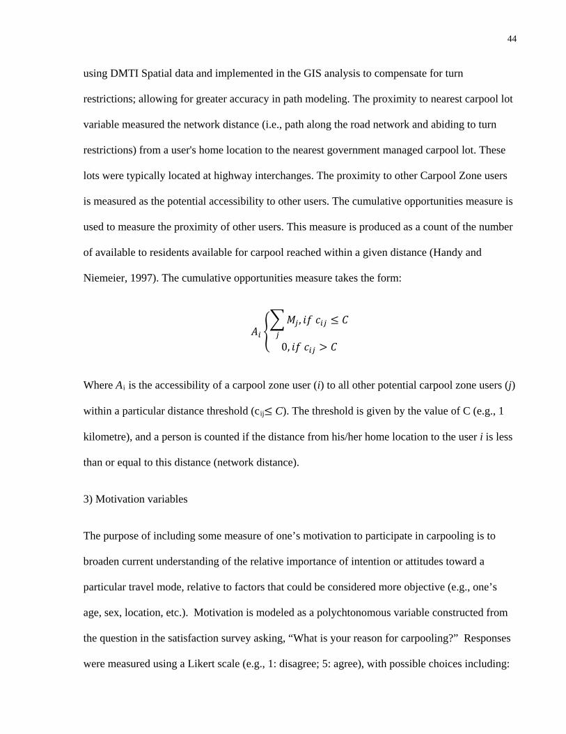
44

using DMTI Spatial data and implemented in the GIS analysis to compensate for turn

restrictions; allowing for greater accuracy in path modeling. The proximity to nearest carpool lot

variable measured the network distance (i.e., path along the road network and abiding to turn

restrictions) from a user's home location to the nearest government managed carpool lot. These

lots were typically located at highway interchanges. The proximity to other Carpool Zone users

is measured as the potential accessibility to other users. The cumulative opportunities measure is

used to measure the proximity of other users. This measure is produced as a count of the number

of available to residents available for carpool reached within a given distance (Handy and

Niemeier, 1997). The cumulative opportunities measure takes the form:

𝐴𝑖 ��𝑀𝑗 , 𝑖𝑓 𝑐𝑖𝑗𝑗

≤ 𝐶

0, 𝑖𝑓 𝑐𝑖𝑗 > 𝐶�

Where Ai is the accessibility of a carpool zone user (i) to all other potential carpool zone users (j)

within a particular distance threshold (c

3) Motivation variables

ij≤ C). The threshold is given by the value of C (e.g., 1

kilometre), and a person is counted if the distance from his/her home location to the user i is less

than or equal to this distance (network distance).

The purpose of including some measure of one’s motivation to participate in carpooling is to

broaden current understanding of the relative importance of intention or attitudes toward a

particular travel mode, relative to factors that could be considered more objective (e.g., one’s

age, sex, location, etc.). Motivation is modeled as a polychtonomous variable constructed from

the question in the satisfaction survey asking, “What is your reason for carpooling?” Responses

were measured using a Likert scale (e.g., 1: disagree; 5: agree), with possible choices including:

45

(1) Environmental concerns; (2) Saving Money (Cost), (3) HOV Lane Use (a proxy for the value

of time), (4) Other, (5) Don’t drive, and (6) Car not available. The last two categories were

combined to produce a mobility constraints category because of the lack of cases in the “Don’t

drive” category.

4) Household Auto-mobility

The literature suggests that being from a household with a relatively higher vehicle per licensed

driver ratio decreases the likelihood of sustainable transport adoption. In this study, however,

attention turns really to the application of household vehicles to carpooling, given that a worker

has decided to participate in a carpool program. Clearly, owning and operating a vehicle has

several out of pocket, and on-going expenses associated with it. It is expected that those with no

household vehicles, will be less likely to succeed in carpooling as they do not have a vehicle to

add to the pool. Individuals with many household vehicles could be more likely to seek out

arrangements to share in the cost of personal vehicle ownership and use. Hypothetically, and in

this case, more vehicles per household could have a positive impact on the construction of a

successful carpool.

5) Scheduling of work

Evidence from the literature suggests temporal regularity of work dictates the decision to carpool

(Cervero & Grisenbeck, 1988; Tsao & Lin, 1999; Ferguson, 1990). A number of studies have

found flex-time programs inhibit the likelihood of carpool formation and typical work schedules

(i.e., 8am - 4pm or 9am - 5pm) favour in carpooling. This research will confirm whether these

observations from the literature match with Carpool Zone users, respondents from an employer-

led carpool scheme. Using data from the trip dataset, a variable was constructed to control for the

46

impact of a regular work schedule on carpooling, in comparison to respondents with shift work

and/or irregular commute schedules. Dummy coding was used to classify respondents

commuting to work five days a week between the hours of 8-4, 8:30-4:30 and 9-5 as having a

typical schedule (coded as 1).

6) Role Preference

Role preference can be divided into either: 1) driving all the time; 2) riding all the time as a

passenger; or 3) sharing driving responsibilities. Levin (1982) illustrated that role preference can

influence carpooling. It was found that users willing to share driving responsibilities were more

successful in forming carpools. Similarly, Buliung et al. (2010) cited users driving or riding all of

the time had less success with the production of carpools, than workers who indicated a

preference for shared responsibilities. The variable concerning role mobility in the trip dataset

was recoded into three separate columns: Share (i.e., those who share driving responsibilities),

Drive (i.e., drive only), Ride (i.e., ride only). Role preference is modeled as a dummy variable,

whereby a user was mutually exclusively coded as "1" as sharing, driving, or riding.

7) Commute distance

Studies have suggested that long commute distances can either encourage or act as a barrier to

carpool formation. Cervero and Griesenbeck (1988) argued that a clerical employee with a

commute distance of 50 miles is twice as likely to carpool if he/she commutes only 4 miles. In

contrast, Lue and Colorni (2009) found that university students preferred traveling at shorter

distances to "park and ride" facilities; rather than a direct commute to their campus because of

greater availability of matches to “park and ride” destinations. In addition, Levin (1982) found

that carpooling desirability decreased with increasing time to pick up and deliver passengers.

47

This study will determine whether or not commute distance impacts the odds of carpool

formation, and if so, whether increasing commute distance advance or discourage the odds.

Commute distances were modeled in logistic regression to determine how carpool formation

varies systematically with distance. The trip dataset, provided by Smart Commute, contained the

return trip distance (km) for each respondent using the 'Carpool Zone' tool. These distances were

inconsistent and not used in the analysis because it was not clear how these distances were

generated. The return distance was based on either, (1) user drawn routes, or (2) a path generated

from within the Carpool Zone software. There was no discernable way of determining which

kind of distance the user generated because of the lack of information. The research required a

consistent commute distance to be obtained. With the aid of the Network Analyst in ArcGIS,

distances between the trip's origin and destination of each respondent from the trip dataset were

generated. Travel time (min) was chosen as the impedance because the shortest travel time

represents a more realistic approach to modeling the shortest path in terms of traffic flow. One-

way and turn restrictions were also controlled for in path estimation.

8) Workplace Characteristics

Smart Commute provided employer data for Carpool Zone users. A firm type from the North

American Industry Classification System (NAICS) was matched to each user. This variable was

further reclassified to associate each user with the broadest economic classification: goods-

producing or service-producing industries. The goods-producing industries are defined as

"primarily associated with the production of goods (e.g., growing crops, generation of electricity,

the manufacturing of computers)" (Industry Statistics, 2011). In contrast, service-producing

industries are but not limited to: professional, scientific, and technical services; finance and

insurance; public administration; and retail trade. Recent statistics suggest Canada's service-

48

producing industries are continuing to increase more rapidly than goods-producing sectors.

Furthermore, the service-producing industries contribute more into Canada's GPD (roughly

70%). This research will study only Carpool Zone users employed in the service-producing

industries. The reason being: 1) outpacing the goods-producing industries; 2) less than 5% of

Carpool Zone users in the workplace dataset belonged to the goods-producing sectors. As a

result, users labeled as goods-producing were removed from the dataset.

The majority of studies on carpooling have recognized that a large workplace could have

greater success in carpool formation than a smaller firm (Cervero and Griesenbeck, 1988;

Ferguson, 1990; Brownstone and Golob, 1992; Teal, 1987). This research will assess whether

users employed at larger firms possess a higher likelihood to carpool because of the greater

opportunities (i.e., number of employees) for finding carpool matches.

Reserved parking based on participation in a TDM program, or for other reasons, offers

highly desirable parking locations near the workplace. A study by Golob (1992) correlated

priority parking with successful carpool formation. The employer dataset provided by Smart

Commute reported the number of carpool spaces at each user's firm. This research hypothesized

that having a greater number of carpool spaces at the firm would increase the odds of carpool

formation.

Both emergency ride home (ERH) and flex-time programmes are transportation demand

management programs offered at workplaces to encourage sustainable transport and alleviate

traffic congestion. ERH is a program that provides users that are participating in a carpooling

program a guaranteed ride home in the case one is not available in the form of cash

reimbursement for a taxi or similar compensation. Flex-time programs provides employees with

flexible work schedules (i.e., outside the typical work hours) to minimize traffic congestion. The

49

literature suggests that ERH programs encourage ridesharing because of the safeguard it provides

a user in case a carpool is not available. Flex-time programs seem to have the opposite effect.

Flex-time acts as a proxy to scheduling of work decreasing the likelihood of carpool formation

due to temporal irregularity of work schedules. Flex-time users commute at atypical works hours

to avoid traffic congestion. In doing so, there are less users/employees available for carpool

matches. With respect to ERH and flex-time, both variables in the workplace dataset are coded

as dichotomous variables.

9) Built Environment Variables

The potential to influence travel behaviour (i.e., mode choice, trip frequency, trip length,

vehicles miles traveled) by altering the built environment is an extensively studied topic in urban

planning. A recent paper suggests that over 200 articles have been published within this research

domain (Ewing & Cervero, 2010). The ultimate goal for urban planners is to understand how to

design neighbourhoods and large cities to reduce automobile dependency, environmental

concerns, and traffic congestion. Three principal dimensions of the built environment (i.e.,

density, diversity, and design) conceived by Cervero and Kockelman (1997) are thought to

influence travel demand. In recent studies, destination accessibility and distance to transit were

also included as additional dimensions affecting travel behaviour (Ewing & Cervero, 2001;

Ewing et al., 2009). These dimensions and how they are measured in this study are described

below.

Density

Population density was measured at both the origin and destination ends at the dissemination

area level (DA). DAs are composed of one or more neighbouring dissemination blocks, with a

50

population of 400 to 700 persons. It is the smallest geographic unit captured in the Canadian

Census. For each respondent, population density was calculated as the population of the DA at

its origin location (or destination) divided by the area of the DA (in squared kilometres). Cervero

and Murakami (2009), revealed that higher population densities in 370 US urbanized areas are

strongly associated with reduced vehicles miles traveled (VMT). The VMT is the total number of

miles driven by all vehicles within a given time period and geographic area. In areas of high

residential densities, a reduction in VMT might occur because of an increase in carpool

propensity. Higher residential densities could correlate with a greater chance to find a match,

simply because of the relatively large concentration of people within close proximity to one

another.

Diversity

With regard to the built environment, diversity, “pertains to the number of different land uses in

a given area and the degree to which they are represented in land area, floor area, or

employment” (Ewing & Cervero, 2010, p. 3). In this study, the Herfindahl-Hirschman entropy

Index (HHI) was chosen to measure land-use mix at each respondent’s origin and destination

locations at varying buffer distances of 500 to 6000 metres (by 500 metre increments). At each

location, the area within each buffer was comprised of some or all of the following land-use

types: commercial government, open area, parks and recreation, residential, resources and

industrial.

In order to calculate the HHI at each location, the areas of each land-use type within the

buffer was determined separately via GIS computation. The next step was to calculate the

proportion of each land-use type within the buffer as a percentage. Using these proportions, the

HHI can be calculated:

51

∑=

⋅=k

iPHHI

1

2)100(

Where k is the number of land-use types, and P is the percentage of each land use type within the

study area (i.e., buffer). The HHI ranges from 0 to 1, moving from a diverse area composed of

many land-use types to a homogeneous designated area.

Design

The design of street networks "vary from dense urban grids of highly interconnected, straight

streets to sparse suburban networks of curving streets forming loops and lollipops" (Ewing and

Cervero, 2010, p.3). Residential street networks in the suburbs are more often closely

characterized by the latter and associated with lower traffic flow. Similarly, street width has the

potential to moderate travel demand since "an increase in street width...lowers densities and

increases travel times between points" as more area is devoted to auto mobility (Southworth &

Ben-Joseph, 2003, p.3). Measures of street design can include: number of intersections per

square kilometre, average block size, proportion of four way intersections, average speed limit,

average street width, and etc. This study will measure the street density in buffers ranging from

500 to 4000 metres (by 500 increments) at each respondent's origin and destination locations.

The street density measure is simply the street length divided by the area of the buffer. The total

length of street network within each buffer is calculated in a GIS by using DMTI CanMap Route

Logistic data. As street density increases, the area becomes more accessible for residents because

more streets are available in the surrounding area to traverse back and forth.

52

Destination Accessibility

Destination accessibility is a recent addition to the original "three Ds" conceived by Cervero and

Kockelman (1997). These built environment dimensions are known to moderate travel demand.

Destination accessibility measures the ease of access to trip attractions (e.g., places of

employment) from a particular location (e.g., origin or destination end). In this study, the

cumulative opportunities measure is used as a measure for destination accessibility. This is

measured by counting the number of places of employment from each respondent's origin and

destination locations at varying buffers (500 to 3500 metres by 500 metres increments).

Significant (i.e., p < 0.1) buffer distances were estimated and identified by means of the bivariate

regression process. Only significant estimates were considered to the next stage of modeling

(i.e., multivariate regression). Two types of cumulative opportunities measures were created to

explain destination accessibility: weighted accessibility and unweighted accessibility. The

weighted measure reports all the number of employees working within the buffer, while the

unweighted reports only the number of businesses within the buffer. The weighted measure

captures the intensity of employment in the area of study, while the unweighted measure

captures the diversity of employment within the area. The cumulative opportunities measure

takes the form:

𝐴𝑖 ��𝑀𝑗 , 𝑖𝑓 𝑐𝑖𝑗𝑗

≤ 𝐶

0, 𝑖𝑓 𝑐𝑖𝑗 > 𝐶�

Where Ai is the destination accessibility of a carpool zone user (i) to all other potential

workplace/employment (j) within a particular distance threshold (Cij≤ C).

53

The threshold is given by the value of C (500m to 3500m), and a business/employment is

counted if the distance from its location to the user i is less than or equal to this distance. The

business GIS data was obtained from Canada Business Data which contained geographic

location information and related attributes for businesses, financial institutions, shopping centres,

general merchandise stores, and grocery stores. Each business was associated with a NAICS

code and the data was filter to only include service-producing businesses.

Distance to Transit

Lastly, the final built environment examined in this study is the distance to transit. It is

hypothesized that shorter distances from a place of residence to transit stops or transportation

hubs will encourage an individual to take public transit than SOV transport. The network

distance to the nearest transit stop is calculated from both the respondent's trip origin and

destination locations using a GIS. Transit stop data was obtained from DMTI Spatial Ltd.

3.2.4 Spatial Modeling

3.2.4.1 Carpooling Hotspots

In this study, a spatial autocorrelation methodology was utilized to examine the spatial processes

of clustering and dispersion across the study area to uncover unique trends and patterns. The

predicted log odds of each respondent generated from the specified multivariate logistic

regression model was used to test for spatial autocorrelation. The predicted odds ratio indicates

the probability of a user to form/not form due to their combined socio-demographic,

motivational, spatial, and workplace characteristics. A large positive odds ratio suggests that the

user is more likely to initiate and use carpools. A map can be constructed to depict areas where

clustering of high or low odds is occurring. Spatial clustering in this study is determined via the

local Moran’s I measure.

54

Local indicators of spatial association (LISA), such as local Moran’s I, serve as indicators

of local pockets of non-stationarity, or hot spots (Anselin, 1994). LISA statistics account for

both the location and value of each feature simultaneously to determine the degree of clustering

or dispersion. In other words, spatial autocorrelation exist when adjacent observations of the

same phenomenon are correlated (either negatively or positively). The local Moran’s I

calculations were performed using ArcGIS 9.3. The specific statistic used here is given by

Anselin (1994):

)( ,2 XxwS

XxI i

n

ij1,jji

i

ii −

−= ∑

≠=

Where xi is an attribute for feature i, X is the mean of the corresponding attribute, jiw , is the

spatial weight between i and j, and:

2,12

1X

n

wS

n

ijjij

i −−

=∑

≠=

with n equating to the total number of features.

In the equation of the local Moran’s I, the numerator represent the covariance of the odds,

while the denominator normalizes the equation. An important component in the equation is the

spatial weight matrix – represented as wij. The spatial weight matrix is a representation of the

spatial structure of the dataset. It defines the spatial relationship that exists among the features

(the respondents). The spatial weight matrix is typically constructed using distance or contiguity

55

approaches. One popular distance-based approach is inverse distance weighting using Euclidean

distance. This method measures the distance of each point (respondent) to all other point

(respondents) in the study area. As a result, the relationship between cases is assumed to

decrease with distance (i.e., Tobler’s law, suggesting that things that are closer in space or more

similar). In this study, network distance is used instead of Euclidean, a less abstract approach and

one that reflects the actual navigation of users through the road transport system.

Once the local Moran’s I values were computed for each respondent, they were

transformed into z-scores to distinguish between clustering of high and low values (Orford,

2004). The following equation illustrates the transformation process:

The iZI score for the statistics are computed as:

][][

i

iii IV

IEIZI −=

where:

1][ ,1

−−=∑

≠=

nIE

n

ijji

22 ][][][ iii IEIEIV −=

Respondents possessing high positive z-scores values are associated with clusters of users with

high carpool odds. Conversely, high negative z-scores values indicate clusters of users with low

odds ratios. Using these values, users holding a z-score of 2 or greater (which is also 2 standard

deviation) were mapped in a GIS to illustrate areas within the GTHA where clustering of high

carpool odds was indicated.

56

3.2.4.2 Autocovariate Regression

Spatial autocorrelation is a phenomenon where values of a variable show a regular pattern over

space. With respect to ordinary least square (OLS), residuals (difference between observed and

predicted values) exhibiting a regular pattern over space may pose a challenge for hypothesis

testing and prediction. This is challenging because it violates the assumption of independently

and identically distributed (i.i.d.) errors of most standard statistical procedures and would inflate

type I errors (Dormann et al., 2007). Type I errors occur when the null hypothesis is wrongly

rejected when in reality there is no evidence for doing so. As a result, this may pose problems in

logistic regression modeling without compensating for spatial effects. Also coefficient signs and

magnitudes can get messed up

A global Moran's I test was conducted to test whether the residuals from the multivariate

logistic regression model exhibit spatial autocorrelation. If spatial autocorrelation does exist, this

would justify for an autologistic regression model to be created that would compensate for the

spatial effects and thus a more reliable model. The global Moran’s I is presented as:

where wij is the weight between observations i and j, and S0 is the sum of all wij. wij represents a

matrix of inverse distance (Euclidean distance) weights. The global Moran’s I analysis was

carried out using R version 2.12.2 using the spdep (Spatial dependence: weighting schemes,

statistics and models) package (R Development Core Team, 2011).

57

An autologistic regression consists of an extra explanatory variable in the model that

captures the effect of other response values in the spatial neighbourhood (i.e., other variables

affecting the response variable that is not included in the model). The autologistic method is

ideal for data with binomial distributed residuals and is known to produce a better fitted model as

demonstrated by Augustin et al (1996). In this study, the autocovariate term was computed as a

weighted average of the number of occupied squares amongst a set of ki neighbours of square i.

The weight given to square j is wij = 1/hij2, where hij

2

1

1

cov

i

i

k

ij jj

i k

ijj

w yauto

w

=

=

=∑

∑

is the squared (Euclidean) distance

between squares i and j. The autocovariate term is described as:

where yj is the response variable.

The autocovariate/autologistic model was generated to be compared to the multivariate model to

observe changes in significance and parameter estimates (in term of direction and size).

58

4 Results This chapter reports the thesis results focusing on: 1) similarities and differences in formed and

non-formed carpools; 2) how various explanatory variables (e.g., spatial, temporal, workplace,

motivational characteristics) associate with carpool formation and use; 3) how/if spatial

autocorrelation has affected the modeling results. The first section (Section 4.1) is a descriptive

analysis of sample data. The next section (Section 4.2) presents both bivariate and multivariate

logistic regression results. The final section introduces a spatial model of carpool formation.

4.1 Sample Exploration The research explores the carpool formation and use process of individuals enrolled in the Smart

Commute’s Carpool Zone program. A satisfaction survey was conducted in late 2007 to evaluate

Carpool Zone’s performance from a total of 4,774 registered users. The survey yielded a sample

of 1,422 responses and was further reduced to 358 respondents after careful data filtering

described in the previous chapter (Chapter 3). The filtering process was necessary for two

reasons: (1) to remove incomplete responses; (2) to isolate for service workers in the employer

program of Carpool Zone. The following section provides a descriptive analysis of the final

sample separated into two groups of users, those who had formed a carpool at the time of

sampling, and those who had not.

4.1.1 Sample Geography

The study area (discussed in Chapter 3) corresponds to the geographic extent Smart Commute’s

TMAs, located across the GTHA. Carpool Zone users (final sample) are heavily concentrated

around the 400 series highway, a network of controlled-access freeways (Figure 5). The majority

of trip origins (e.g., home location) are situated within the Peel region (i.e., Mississauga and

Brampton & Caledon) and downtown Toronto. Trip destinations, however, are mainly

59

concentrated outside the City of Toronto census division and in suburban areas. The lack of

destinations within central Toronto was due to the removal of all respondents associated with the

Smart Commute Toronto-central TMA during the data filtering process. These respondents had

no employment characteristics (i.e., type of firm, firm size, number of carpool spaces at firm,

ERH availability, flex time availability) attached to them because the Smart Commute Toronto-

central TMA did not exist at the time of survey. The distribution of respondents at the home end

in each Smart Commute TMA across the GTHA is summarized in Table 3.

Smart Commute TMA # of Respondents

Markham & Richmond Hill 38

Brampton & Caledon 50

Durham 19

Halton 32

Hamilton 13

Mississauga 132

Northeastern Toronto 3

North Toronto, Vaughan 50

Central York 21

Toronto-Central 0

Table 3 Distribution of Respondents by Trip Destination in each Smart Commute TMA

The following is a brief demographic outline of the final sample (n=358): 121 users (33.8%) of

the final sample had successfully formed carpools, whereas the remaining 237 users (66.2%) had

not formed carpools at the time of survey. The average age of the respondents was 36 years. The

average household income (DA-level) was $74,246.38, which closely resembles the 2007

national average household income in Canada of $73,700 (Statistics Canada, 2009). However,

the sample is biased towards high income because the sample selection included only those from

the service sector and employer-based users of Smart Commute. In addition, it is worth noting

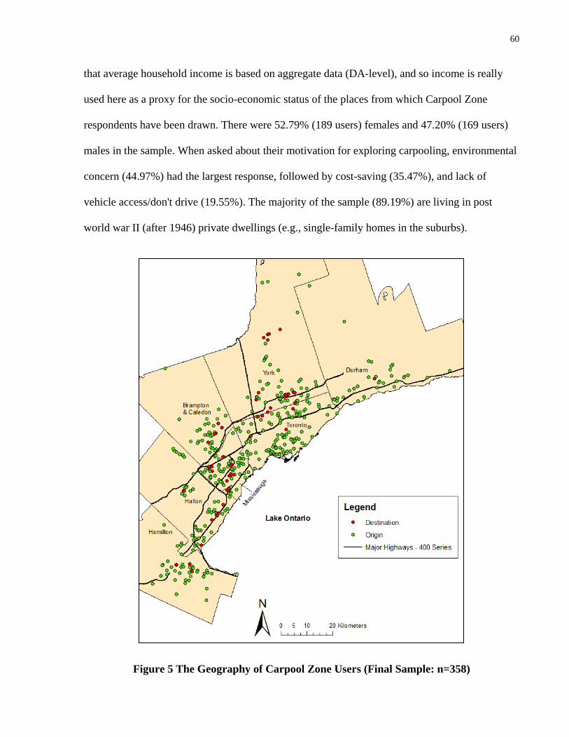
60

that average household income is based on aggregate data (DA-level), and so income is really

used here as a proxy for the socio-economic status of the places from which Carpool Zone

respondents have been drawn. There were 52.79% (189 users) females and 47.20% (169 users)

males in the sample. When asked about their motivation for exploring carpooling, environmental

concern (44.97%) had the largest response, followed by cost-saving (35.47%), and lack of

vehicle access/don't drive (19.55%). The majority of the sample (89.19%) are living in post

world war II (after 1946) private dwellings (e.g., single-family homes in the suburbs).

Figure 5 The Geography of Carpool Zone Users (Final Sample: n=358)

61

4.1.2 Formed versus Non-Formed

The Smart Commute satisfaction survey (conducted in late 2007) required respondents to report

their usage level of Carpool Zone. Respondents classified as “formed” are users that had formed

and started carpooling at the time of survey. In this study, non-formed users were considered any

of the following: waiting for a match, waiting for better match, waiting on response, or formed

without starting. Kernel density mapping is a technique used to visualize the magnitude per unit

area from point features (i.e., origin locations) using a kernel function to fit a smooth surface to

each point. The approach is used here to explore the regional trend in the distribution of users by

their “formed”, “non-formed” status (Figure 6). The non-formed group appears to be more

regionally dispersed, having a larger presence in the City of Mississauga and the City of Toronto.

Conversely, the formed group is less regionally dispersed, and highly concentrated within central

Toronto and western Toronto (i.e., High Park neighbourhood).

62

Figure 6 Comparison of Non-formed vs. Formed Kernel Density Maps

63

A descriptive statistical analysis was conducted to make comparisons between the formed

and non-formed groups. The thesis attempts to identify key differences between the groups to

provide policy planners with a greater understanding of the process affecting carpool formation

to refine strategies that increase carpool propensity. The following section summarizes the

results by comparing averages and proportions of various variables between the groups.

Table 4 Descriptive Statistics of Continuous Variables for Form and Non-Formed Groups

Continuous Variable Formed Non-Formed t dfSig. (2-tailed)

Age 36.818 35.084 -1.508 356.000 0.133Income ($ CND) 76952.579 72864.734 -1.349 356.000 0.178

Number of Household Automobiles 1.521 1.354 -1.609 356.000 0.109Commute Distance (km) 32.211 28.909 -1.583 356.000 0.114Firm Size (# employees) 4083.694 11857.388 4.626 355.820 0.000

Carpool Spaces 10.529 4.561 -5.360 193.362 0.000Population Density - Origin (# people/km2) 4840.752 5640.205 1.301 314.744 0.194

Population Density - Destination (# people/km2) 1814.113 3463.519 2.669 336.216 0.008Nearest Transit Stop - Origin (metres) 2971.151 2649.173 -1.387 356.000 0.166

Nearest Transit Stop - Destination (metres) 2209.089 2021.646 -1.144 356.000 0.253Street Density - Origin - 2500m (m/km2) 9.400 8.780 -1.977 356.000 0.049

Street Density - Destination - 500m (m/km2) 8.694 9.375 2.314 356.000 0.021HHI - Origin (500m) 0.548 0.576 1.360 356.000 0.175

HHI - Destination (500m) 0.461 0.427 -2.109 220.790 0.036Cumulative Opportunities - Weighted - Origin -2500m

(# of workers) 55151.091 36567.274 -1.582 161.683 0.116Cumulative Opportunities - Weighted - Destination -

3500m (# of workers) 57245.587 76487.363 6.264 294.138 0.000

Mean

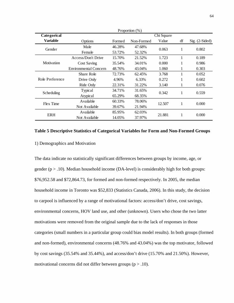
64

Table 5 Descriptive Statistics of Categorical Variables for Form and Non-Formed Groups

1) Demographics and Motivation

The data indicate no statistically significant differences between groups by income, age, or

gender (p > .10). Median household income (DA-level) is considerably high for both groups:

$76,952.58 and $72,864.73, for formed and non-formed respectively. In 2005, the median

household income in Toronto was $52,833 (Statistics Canada, 2006). In this study, the decision

to carpool is influenced by a range of motivational factors: access/don’t drive, cost savings,

environmental concerns, HOV land use, and other (unknown). Users who chose the two latter

motivations were removed from the original sample due to the lack of responses in those

categories (small numbers in a particular group could bias model results). In both groups (formed

and non-formed), environmental concerns (48.76% and 43.04%) was the top motivator, followed

by cost savings (35.54% and 35.44%), and access/don’t drive (15.70% and 21.50%). However,

motivational concerns did not differ between groups (p > .10).

Categorical Variable Options Formed Non-Formed

Chi Square Value df Sig. (2-Sided)

Male 46.28% 47.68%Female 53.72% 52.32%

Access/Don't Drive 15.70% 21.52% 1.723 1 0.189Cost Saving 35.54% 34.01% 0.000 1 0.986

Environmental Concern 48.76% 43.04% 1.060 1 0.303Share Role 72.73% 62.45% 3.768 1 0.052Drive Only 4.96% 6.33% 0.272 1 0.602Ride Only 22.31% 31.22% 3.140 1 0.076Typical 34.71% 31.65%Atypical 65.29% 68.35%Available 60.33% 78.06%

Not Available 39.67% 21.94%Available 85.95% 62.03%

Not Available 14.05% 37.97%ERH

Gender

Motivation

Role Preference

Scheduling

Flex Time

0.342 1 0.559

Proportion (%)

0.063 1 0.802

12.507 1 0.000

21.881 1 0.000

65

2) Workplace

There were significant between group differences regarding workplace transport context. The

average number of carpool spaces is nearly double for the formed group compared to the non-

formed group (10.53 vs. 4.56 spaces, p < 0.01). With respect to firm size, the results revealed the

formed group had a larger mean firm size than the non-formed group (11857.39 versus 4083.69

employees, p < 0.01). Users from the formed group reported having more cars per household, on

average, (1.52) compared to the non-formed group (1.35) (p > 10). No differences in commute

distance or work scheduling were detected (p > .10). Between groups, differences were found for

role preference. Those willing to share roles (drive or ride) were more likely to belong to the

formed (72.72%) rather than non-formed (62.00%) group. Individuals looking to ride only were

more likely to be in the non-formed group (31.22%) versus 22% the formed group (22%).

Differences in workplace availability of TDM programs between the groups were also

looked at. The specific TDM options included emergency ride home, and flex time. Statistically

significant differences were found between the formed (85.95%) and non-formed (62.03%)

groups for ERH availability (p < 0.01). Similarly, a substantial difference is observed between

those with and without flex time at their workplace. More users with flex time (p < 0.01) at their

firm belonged to the non-formed group (78.06%) compared to the formed group (60.03%).

3) Built Environment

The built environment is expected to associate with carpooling. Built environment measures

included in this thesis are: population density, street design, land-use diversity, destination

accessibility, and distance to nearest transit stop. The Herfindahl–Hirschman Index (HHI) is

applied to measure the land use diversity of the area surrounding each user’s origin and

66

destination locations. An HHI value near zero indicates a highly diverse or heterogeneous

landscape, whereas a value near one corresponds with a more homogeneous situation. The

descriptive summary reported that only the HHI destination-end is significant, with an indication

of less diversity for the formed (0.46) versus the non-formed (0.43) group (p < 0.05). Population

density was higher, at the destination end, for the non-formed (3463.52 persons/km2) than for the

formed (1814.11 persons/km2) group (p < 0.01). No difference was observed for population

density at the trip origin. The mean street density at both the origin and destination ends

displayed statistically significant values. Street density at the origin is denser for the formed

group (9.40 m/km2 versus 8.78 m/km2) than the non-formed group (p < 0.05). Street density at

the destination end is denser within the non-formed group (9.38 m/km2 versus 8.69 m/km2

4.2 Logistic Regression

) than

the formed group (p < 0.05). A cumulative opportunity measure was used to evaluate the

accessibility of employment from each user’s trip origin and destination locations. At the

destination, the mean cumulative opportunities was found to be greater for the non-formed group

compared to the formed group (76487.36 employees vs. 57245.59, p < 0.01). Lastly, no between

group differences were detected in terms of transit access.

Logistic regression models can be specified to examine the relationship between a dependent

variable and one (bivariate) or more independent variables (multivariate). This thesis uncovers

the relative influences of the following independent variables on carpool formation: demographic

characteristics, spatial factors, motivation for carpooling, household auto-mobility, scheduling of

work, commute distance, role preference, workplace characteristics, and the built environment.

This particular study is most concerned with the latter set of independent variables (i.e., built

environment) since the other sets of variables have been examined in past research (Buliung et

67

al., 2010). The first section of this chapter reports the bivariate regression results. Bivariate

relationships were tested as part of a variable filtering process. Bivariate unadjusted regressions

were fit in an attempt to reduce the lengthy set of possible correlates down to those most likely to

explain systematic variation in the response variable once included in the multivariate models.

Only those variables holding a statistical significance at p ≤ 0.10 from the bivariate regressions

were included in the adjusted multivariate models. Variable descriptions are shown in Table 2. A

parsimonious approach was taken for model specification, to ensure that the models were not

over-specified (i.e., too many variables relative to the number of cases) (Peduzzi et al., 1996).

4.2.1 Bivariate Results

Bivariate regressions (Table 6) were conducted between the response variable (carpool usage)

and each independent variable. The response variable is a dichotomous variable whereby users

that have formed and started using carpools are designated as “1” and non-formed users are

assigned “0”. The independent variables are comprised of both continuous and categorical

variables. The statistically significant variables generated from the bivariate regressions form the

pool of possible independent variables for the multivariate regression models. In Table 6, those

variables in bold typeface are considered statistically significant (p ≤ 0.10) and processed to the

next stage of data filtering (i.e., multi-colinearity). For those variables where characteristics were

measured repeatedly at different geographical distances (e.g., proximity to other users), only the

most significant variable (i.e., lowest p-value) among the group was chosen.

68

Table 6 Bivariate Regressions - Carpool Formation

Variable P-Value BetaGender 0.80206 0.05614Age 0.13309 0.01612Income 0.17871 0.00001Proximity to Users - 500 metres 0.13420 0.15585Proximity to Users - 1000 metres 0.02151 0.11827Proximity to Users - 1500 metres 0.07071 0.04974Proximity to Users - 2000 metres 0.01048 0.04763Proximity to Users - 2500 metres * 0.00785 0.03584Proximity to Users 3000 metres 0.04027 0.02118Proximity to Users 3500 metres 0.05147 0.01590Distance to Nearest Carpool Lot * 0.00935 0.00003Don't Drive or No Access 0.33223 -0.31777Environmental Concerns 0.62340 0.12218Number of Household Automobiles 0.10936 0.19364Drive Only 0.60257 -0.25855Ride Only 0.07769 -0.45777Network Trip Distance 0.11503 0.00936Scheduling 0.55876 0.13833Urban 0.12766 0.36920Intra vs. Inter Zonal Commute 0.18554 -0.32542Firm Size * 0.00085 -0.00003Number of Carpool Spaces at Firm * 0.00000 0.06311Emergency Ride Home * 0.00001 1.32055Flex Time * 0.00048 -0.84985Population Density Origin 0.24328 -0.00002Population Density Destination * 0.02601 -0.00005Nearest Transit Stop (metres) - Origin 0.16839 0.00007Nearest Transit Stop (metres) - Destination 0.25298 0.00009Herfindahl-Hirschman Index - Origin - 500 metres 0.17487 -0.84711Herfindahl-Hirschman Index - Origin - 1000 metres 0.17969 -0.99218Herfindahl-Hirschman Index - Origin - 1500 metres 0.39258 -0.69776Herfindahl-Hirschman Index - Origin - 2000 metres 0.97411 -0.02803Herfindahl-Hirschman Index - Origin - 2500 metres 0.89592 0.11689Herfindahl-Hirschman Index - Origin - 3000 metres 0.97066 0.03350Herfindahl-Hirschman Index - Origin - 3500 metres 0.89142 -0.12525Herfindahl-Hirschman Index - Destination - 500 metres * 0.03208 1.65884Herfindahl-Hirschman Index - Destination - 1000 metres 0.63021 0.42705Herfindahl-Hirschman Index - Destination - 1500 metres 0.78669 0.25512Herfindahl-Hirschman Index - Destination - 2000 metres 0.35117 0.83672Herfindahl-Hirschman Index - Destination - 2500 metres 0.44693 0.81556Herfindahl-Hirschman Index - Destination - 3000 metres 0.71641 0.46097Herfindahl-Hirschman Index - Destination - 3500 metres 0.72283 0.50959

69

Table 6 (continued) Bivariate Regressions - Carpool Formation

The results of the bivariate logistic regressions conform to the literature with respect to

the role of socio-economic and demographic characteristics on the carpooling decision (Canning

et. al, 2010; Benkler, 2004; Kaufman, 2000; Teal, 1987; Horowitz and Sheth 1978; Ferguson,

Variable P-Value BetaStreet Density - Origin - 500 metres 0.32264 0.03590Street Density - Origin - 1000 metres 0.09812 0.06353Street Density - Origin - 1500 metres 0.06460 0.07326Street Density - Origin - 2000 metres 0.05110 0.07912Street Density - Origin - 2500 metres * 0.04996 0.08071Street Density - Origin - 3000 metres 0.07997 0.07294Street Density - Origin - 3500 metres 0.11289 0.06618Street Density - Destination - 500 metres * 0.02237 -0.09818Street Density - Destination - 1000 metres 0.73670 0.01523Street Density - Destination - 1500 metres 0.85587 0.00873Street Density - Destination - 2000 metres 0.32521 0.05273Street Density - Destination - 2500 metres 0.28427 0.06792Street Density - Destination - 3000 metres 0.42279 0.05645Street Density - Destination - 3500 metres 0.91281 0.00838Cumulative Opportunities - Unweighted - Origin - 500 metres 0.25224 0.00037Cumulative Opportunities - Unweighted - Origin - 1000 metres 0.20791 0.00016Cumulative Opportunities - Unweighted - Origin - 1500 metres 0.23753 0.00008Cumulative Opportunities - Unweighted - Origin - 2000 metres 0.08568 0.00008Cumulative Opportunities - Unweighted - Origin - 2500 metres * 0.05257 0.00007Cumulative Opportunities - Unweighted - Origin - 3000 metres 0.05913 0.00005Cumulative Opportunities - Unweighted - Origin - 3500 metres 0.06316 0.00004Cumulative Opportunities - Weighted - Origin - 500 metres 0.26934 0.00001Cumulative Opportunities - Weighted - Origin - 1000 metres 0.25330 0.00000Cumulative Opportunities - Weighted - Origin - 1500 metres 0.34687 0.00000Cumulative Opportunities - Weighted - Origin - 2000 metres 0.13592 0.00000Cumulative Opportunities - Weighted - Origin - 2500 metres * 0.08412 0.00000Cumulative Opportunities - Weighted - Origin - 3000 metres 0.08617 0.00000Cumulative Opportunities - Weighted - Origin - 3500 metres 0.09184 0.00000Cumulative Opportunities - Unweighted - Destination - 500 metres 0.36124 -0.00095Cumulative Opportunities - Unweighted - Destination - 1000 metres 0.03350 -0.00115Cumulative Opportunities - Unweighted - Destination - 1500 metres 0.00012 -0.00124Cumulative Opportunities - Unweighted - Destination - 2000 metres 0.00000 -0.00102Cumulative Opportunities - Unweighted - Destination - 2500 metres 0.00000 -0.00094Cumulative Opportunities - Unweighted - Destination - 3000 metres * 0.00000 -0.00073Cumulative Opportunities - Unweighted - Destination - 3500 metres 0.00000 -0.00055Cumulative Opportunities - Weighted - Destination - 500 metres 0.00755 -0.00011Cumulative Opportunities - Weighted - Destination - 1000 metres 0.00174 -0.00009Cumulative Opportunities - Weighted - Destination - 1500 metres 0.00585 -0.00003Cumulative Opportunities - Weighted - Destination - 2000 metres 0.00037 -0.00003Cumulative Opportunities - Weighted - Destination - 2500 metres 0.00000 -0.00003Cumulative Opportunities - Weighted - Destination - 3000 metres 0.00000 -0.00003Cumulative Opportunities - Weighted - Destination - 3500 metres * 0.00000 -0.00002

70

1997). The demographic characteristics (i.e., gender, age, and income) measured in this study

were all insignificant (p ≥ 0.1) and gender being the most insignificant (p = 0.802).

Both spatial/proximity variables (proximity to users and distance to nearest carpool lot)

examined in this study had high significance but due to their low beta values, and hence low

odds ratios, they had little effect on the decision to carpool. Motivation, household auto-

mobility, work scheduling, commute distance, and role preference were also insignificant.

Workplaces characteristics and built environment characteristics appeared to associate with

carpooling. Firm size and flex time availability produced negative betas from the bivariate

regressions. This suggests that carpool formation for this sample occurred at smaller firms.

Similarly, flex-time availability appears to work against carpool formation. In contrast, number

of carpool spaces, and availability of an Emergency Ride Home program had positive

associations with carpool formation. Firms with greater number of carpool spaces will increase

the probability of employees forming carpools at the workplace. The availability of the

Emergency Ride Home (ERH) program has the greatest effect (i.e., largest beta value) on

carpool formation amongst the workplace characteristics. When ERH is made available at the

workplace, a user’s decision to carpool drastically increases.

Distance to nearest transit stop was the only built environment variable not significant in

the bivariate regressions. Population density is only significant at the destination end and had a

negative association with carpooling. The Herfindahl-Hirschman index is used to measure land

use diversity. The results revealed that diversity at the destination-end (500 metre buffer)

displayed the largest positive beta (beta = 1.65884) among all variables. This implies that greater

uniformity at the destination-end increased the odds of carpool formation. Street density is

measured as the length of street (m) per buffer area (km2). Street density at the origin had a

71

positive association with carpooling. In contrast, at the destination-end, street density had a

negative association with carpool formation. A cumulative opportunities measure is used as a

measure of destination (i.e., employment) accessibility. The cumulative opportunities

surrounding the origin and destination for both weighted and unweighted cases are statistically

significant. Only the destination-end measures were found to have negative betas. People

working at places with a larger number of opportunities located around the destination appeared

less likely to carpool. This suggests there will be less likely chance carpools will be formed when

there are more opportunities for employment at the destination end.

Following this bivariate analysis, tests for multicollinearity between the variables that had

statistically significant relationships. This was done to ensure that collinear (related) variables

were not entered into the linear predictor specified for the multivariate logistic regression

analyses that follow. Multicollinearity results from strong correlation between pairs of

independent variables, having related variables in the linear predictor of a regression model can

produce biased parameter estimates, and incorrect associations. The occurrence of this

phenomenon would inflate the variance of the parameter estimates (Farrar & Robert, 1967).

Appropriate tests were run to examine collinearity between the categorical and continuous

variables. The results indicate correlation between TDM variables (ERH or flex-time

availability), ERH was chosen since it displayed the strongest explanatory power (against flex

time) in the bivariate regressions. Following similar tests between continuous variables, several

environmental variables remained including: distance to nearest carpool lot, firm size, number of

carpool spaces, population density (destination-end), Herfindahl Hirschman Index (destination-

end @ 500m), street density (origin-end @ 2500m), street density (destination-end @ 500m),

cumulative opportunities (weighted – destination @ 2500m), and cumulative opportunities

72

(weighted – origin @ 3500m). The multivariate logistic regression results are the subject of the

remainder of this chapter.

4.2.2 Multivariate Results

The multivariate regression model (Table 7) incorporates the most significant independent

variables from the bivariate models and accounts for multi-colinearity by removing highly

correlated variables to form a parsimonious model. Model fit is acceptable given the number of

variables and sample size. The estimation allows us to better understand the characteristics that

lead to the formation and usage of carpools among Carpool Zone users while controlling for a

variety of demographic, motivational, trip, employment, spatial, and built environment variables.

The constant is the log odds of the outcome (i.e., carpool formation) when all other independent

variables in the model are zero (i.e., having no effect on the response variable). The odds ratio of

the constant (0.062) suggests carpool formation is 93.8% less likely to occur when all

independent variables are set to zero (i.e., belonging to the reference group). The socio-

demographic variables in the multivariate model coincide with the literature that these variables

have little effect on carpooling (Canning et al, 2010; Ferguson, 1997). The only blocks of

variables incorporated into the multivariate model were: spatial, workplace, and built

environment characteristics. The variables that were significant (p ≤ 0.1) in the model included:

distance to nearest carpool lot, firm size, number of carpool spaces, and Emergency Ride Home

(p=0.134). Even though ERH is above the significance threshold, the value explanatory power of

ERH (odds ratio) is worth noting. The distance to nearest carpool lot variable was reported to

have equal odds (OR = 1) for a one-unit increase in distance. Similarly, the odds ratio of the

number of carpool spaces variable was determined to be 1.036 or suggesting carpool formation is

3.6% more likely to occur for each additional carpooling parking space. Emergency Ride Home

(ERH) had the strongest effect on carpool formation in the model with an odds ratio of 2.00 or

73

implying carpool formation is 100% more likely to occur if the firm has an ERH program

available at their workplace. The multivariate model is parsimonious but does not compensate

for spatial autocorrelation. Models that do not account for spatial autocorrelation may result in

bias significance and parameter estimates. The next subsection (i.e., spatial modeling) will

attempt to improve non-spatial regression modeling to control for spatial effects.

Table 7 Multivariate Regression - Carpool Formation

4.3 Spatial Modeling Regression models exhibiting spatial autocorrelation can be problematic if not accounted for in

simple logistic regression because it violates the assumption of independently and identically

distributed (i.i.d.) errors and could lead to biased parameter estimates. In order to compensate for

spatial autocorrelation in logistic models, Augustin et al. (1996) developed a method,

β p-value OR Lower UpperConstant** -2.773 0.040 0.062Age 0.006 0.634 1.006 0.981 1.032Gender 0.076 0.772 1.079 0.645 1.805Income*** 0.000 0.066 1.000 1.000 1.000Distance to Nearest Carpool Lot* 0.000 0.000 1.000 1.000 1.000Firm Size** 0.000 0.032 1.000 1.000 1.000# of Carpool Spaces** 0.035 0.016 1.036 1.006 1.066Population Density - Destination 0.000 0.908 1.000 1.000 1.000HHI - Destination - 500 m 0.411 0.677 1.508 0.218 10.418Street Density - Origin - 2500 m 0.068 0.186 1.070 0.968 1.183Street Density - Destination - 500m -0.035 0.542 0.966 0.865 1.079Cumulative Opportunities - Origin - Weighted - 2500 m 0.000 0.967 1.000 1.000 1.000Cumulative Opportunities - Destination - Weighted - 3500 m*** 0.000 0.087 1.000 1.000 1.000Emergency Ride Home 0.693 0.134 2.000 0.808 4.951

Summary StatisticsNumber of Cases 358.00-2[L(0)-L[β] 381.33x² 76.69NOTES: OR: Odds Ratio, 95% CI: Confidence Interval, HHI: Herfindahl-Hirschman Index*p < 0.01, **p < 0.05, ***p < 0.1

OR +/-95%CI

74

autocovariate regression, to include an extra explanatory term to capture the effect of other

responses values in the spatial neighbourhood. In effect, this would make the residuals of the

model more spatially random and lead to a better fitted model.

The results from spatial modeling are divided into two sections: 1) identifying carpool

hotspots using the predicted log odds generated from the multivariate model; 2) conduct, if

necessary, autocovariate regression to compensate for spatial autocorrelation found in the

residuals of the multivariate regression model. The purpose of mapping carpool hotspots is to

provide insight into the geographic pattern of carpool outcomes. As discussed in previous

sections, the multivariate model is the most parsimonious because it incorporates the ideal

independent variables to produce a model that best fit or explain the carpool formation and usage

process. The equation derived from the multivariate model was used to generate the predicted

odds ratio for each respondent from the sample. Using these predicted odds, carpool hotspots can

be generated using local Moran’s I.

4.3.1 Carpool Hotspots

The following maps illustrate three possible carpooling hotspots that can occur in the GTHA

according to the multivariate model. These hotspots are situated in: Brampton (Figure 7), North

Eastern Toronto (Figure 8), and Central Toronto (Figure 9). For each map, only users that

clustered with high positive odd ratios (i.e., identified using a local Moran’s I and holding a z-

score of 2 or greater) were mapped. Euclidean lines were created between each user’s trip origin

and destination to illustrate type of commutes with high odds (e.g., suburb to suburb, reverse,

etc.).

The Brampton carpool hotspot observed in Figure 7 depicts a large cluster of users

residing within the Bramelea area and commuting at short distances to their workplace. A

75

majority of the users are traveling to Bramelea City Centre shopping mall. A cluster of users

with high positive odds living in North Eastern Toronto is seen in Figure 8. These users are

commuting long distances to workplaces in other municipalities. A large number of users from

this hotspot are commuting to industrial parks such as the Sheridan Science and Technology

Park. Similarly, users from the carpooling hotspot in central Toronto (Figure 9) are also

commuting longer distances (crossing municipal boundaries) and to business parks (e.g.,

Meadowvale Business Park). Industrial parks are zoned and planned for offices and light

industry, whereas business parks consist of grouped commercial buildings. Industrial parks may

have a combination of goods-producing and service-producing industries, while business parks

are exclusively zoned for services-producing industries (Frej, 2001). The study is biased toward

business parks since the sample selection consist of only workers from service-producing

sectors. The findings from the carpooling hotspot analysis will be discussed in greater detail in

Chapter 5.

76

Figure 7 Brampton Carpool Hotspot

77

Figure 8 North Eastern Toronto Carpool Hotspot

78

Figure 9 Central Toronto Carpool Hotspot

79

4.3.2 Spatial Autocovariate Regression Results

Theory about spatial autocorrelation is often linked to Tobler's first law of geography:

"Everything is related to everything else, but near things are more related than distant things"

(Tobler, 1970). In other words, positive autocorrelation occurs when nearby or neighbouring

areas are more similar and vice versa for negative autocorrelation. Spatial autocorrelation has

implications in simple linear regression because it violates the assumption that values of

observation in each user/respondent are independent of one another and this could lead to bias

parameter estimates and error terms.

One of the most common measures of spatial autocorrelation is global Moran's I. A

global Moran’s I test is conducted for the residuals of the multivariate model to assess the need

to carry out autologistic/autocorvariate regression (i.e. determine whether the residuals are

spatial autocorrelated). Moran's I values can be transformed to Z-scores in which values greater

than 1.96 or smaller than −1.96 indicate spatial autocorrelation that is significant at the 5% level.

The results reported a global Moran's I standard deviate (z-score) of 2.211 with p-value of 0.013.

This indicates the residual of the multivariate model is positively spatial autocorrelated. The low

p-value (p < 0.1) indicates rejection of the null hypothesis that assumes spatial randomness of the

residuals. As a result, an autocovariate model was constructed to compensate for spatial effects

(i.e., spatial autocorrelation).

Table 8 reports the results from the autocovariate regression. The model has the same

response variable and explanatory/independent variables as the multivariate regression model. A

global Moran’s I test was conducted on the residuals produced by the autocorvariate model to

determine whether the residuals were spatial autocorrelated. As predicted, the autocovariate

model did not exhibit spatial autocorrelation (spatial effects are adequately controlled for in this

80

model). The Moran's I standard deviate (z-score) was reported to be -0.5645 and p-value =

0.7138 which suggest spatial randomness of the model’s residual. The -2 log likelihood was

reported to be 375.56, lower than the multivariate model (381.33). This suggests the

autocovariate model is better at explaining the relationship between carpool formation and use

and the selected independent variables because of improved model fit. Both regression models

(i.e., multivariate vs. autocovariate) share similar results. Distance to nearest carpool lot, firm

size, and number of carpool spaces all are statistically significant (p-value < 0.1) but their odds

ratio is equal/close to one (to suggest equal probability or no effect on the response variable).

The differences, however, is observed in the constant. The constant is significant in the

autovariate (p-value = 0.019) but not in the multivariate model (p-value = 0.161). The

Emergency Ride Home (ERH) is still insignificant in the autocovariate model (p=0.136) but the

large effect size makes it worth mentioning. The ERH suggest that respondents are 101.4% more

likely to carpool if ERH is available at his/her workplace. Lastly, the extra explanatory variable

in the model, the autocovariate term, is highly significant and has a high odds ratio. This

suggests other spatial processes are affecting the model that were not observed by the researcher.

Possible explanations for this phenomenon are explored in the next chapter (Discussion).

81

Table 8 Autocovariate Regression - Carpool Formation

β p-value OR Lower UpperConstant** -3.252 0.019 0.039 0.003 0.580Age 0.002 0.853 1.002 0.977 1.029Gender 0.049 0.853 1.050 0.625 1.764Income*** 0.000 0.054 1.000 1.000 1.000Distance to Nearest Carpool Lot* 0.000 0.001 1.000 1.000 1.000Firm Size** 0.000 0.022 1.000 1.000 1.000# of Carpool Spaces** 0.037 0.011 1.038 1.009 1.069Population Density - Destination 0.000 0.853 1.000 1.000 1.000HHI - Destination - 500 m 0.636 0.523 1.888 0.268 13.289Street Density - Origin - 2500 m 0.061 0.236 1.063 0.961 1.175Street Density - Destination - 500m -0.036 0.526 0.964 0.862 1.079Cumulative Opportunities - Origin - Weighted - 2500 m 0.000 0.962 1.000 1.000 1.000Cumulative Opportunities - Destination - Weighted - 3500 m 0.000 0.184 1.000 1.000 1.000Emergency Ride Home 0.700 0.136 2.014 0.803 5.050Autocovariate** 1.261 0.017 3.528 1.258 9.894

Summary StatisticsNumber of Cases 358-2[L(0)-L[β] 375.56x² N/ANOTES: OR: Odds Ratio, 95% CI: Confidence Interval, HHI: Herfindahl-Hirschman Index*p < 0.01, **p < 0.05, ***p < 0.1

OR +/-95%CI

82

5 Discussion The thesis extends an ongoing study of the carpool formation and use process in the Greater

Toronto and Hamilton Area (GTHA), Canada’s largest urbanized region. Previous work did not

investigate how workplace characteristics (e.g., firm size, ERH, flex-time, firm type) and the

built environment (i.e., density, diversity, design, distance to nearest transit, and destination

accessibility) associate with carpooling. However, it is important to note that the sample is highly

specialized (i.e., individuals enrolled in the employer-based Smart Commute program and users

are from the service sector). The study is concerned with this particular sample and it is not

intended to be a labour force wide study of carpooling using a wide range of tools beyond Smart

Commute's Carpool Zone. Furthermore, studies concerning carpooling have not adequately

controlled for spatial effects (i.e., spatial autocorrelation) in regression modeling techniques

(e.g., logistic regression). Residuals from a logistic regression model may be spatially

autocorrelated, violating the assumption that residuals are independent and identically

distributed. Regression models that do not account for this problem can potentially produce

misleading parameter estimates. The research also makes a contribution to practice. The results

will assist Smart Commute, a workplace-based transportation demand management (TDM)

program, with their ongoing development of policy and programs aimed at increasing carpool

propensity in the GTHA.

This chapter provides a discussion of the results, situating them within the carpool and

TDM literatures. Explanations are discussed for the results observed from the sample and

implications it has on carpool formation and usage in the GTHA. The chapter is divided in the

following sections: (Section 5.1) makes comparison between users that have formed and not-

formed operating carpools. Next, the multivariate model (Section 5.2) is discussed to understand

83

the underlying carpool formation process. The significance and effect magnitude of the

explanatory variables from the multivariate model will guide planners/researchers in policy

making. The next section (Section 5.3), analyzes the carpool hotspot maps generated from the

predicted odds ratio of each respondent derived from the multivariate model. Lastly (Section

5.4), the issue of spatial autocorrelation is tackled and an explanation on the effect it has on the

modeling results is discussed. Moreover, the study will examine the spatial modeling technique

(i.e., autocovariate modeling) to compensate for spatial autocorrelation and what implications it

has on the modeling results.

5.1 Formed versus Non-formed From a total of 4,774 registered users, only 1,422 users responded to the Carpool Zone

Satisfaction survey. The sample was reduced to 358 respondents to select only service workers

that were participating in the employer-based program of Carpool Zone. The rapid growth rate

and dominance of the service sector in Canada's GDP led to the decision to choose only service

workers in the sample for the study. Public users of carpool zone were not the focus of this

particular study because the research aims to improve employer-based carpool programs and past

research has shown these programs have been most effective (Canning et al., 2010; Buliung et

al., 2010).

In terms of socio-demographic characteristics, many studies have found little or no

association between these attributes (i.e., gender, income, age) and carpool formation (Canning

et. al, 2010; Benkler, 2004; Kaufman, 2000; Horowitz and Sheth 1978; Ferguson, 1997; Buliung

et. al, 2010). Horowitz and Sheth (1978) constructed a ride sharing model for the Chicago area in

1975 and found demographic characteristics (i.e., gender, income, education) were poor

indicators and predictors of the choice between driving alone and ride sharing. Similarly,

84

Canning et al. (2010) observed participants in employer-led carpools with diverse age, income,

and gender to suggest little socio-demographic correlation with the propensity to carpool. The

results from this study reflect the findings argued in the literature.

The proportion of males and females in both groups (formed vs. non-formed) were nearly

identical, suggesting that gender differences do not play a role in the decision to carpool.

Ferguson (1997) found that gender has little association with carpool formation but rather

household composition. More importantly, the study argued that women with small children are

significantly more likely to form household-based carpool, whereas men are neither more nor

less likely to form household-based carpools. The lack of information on household composition

(e.g., number of young children) in the Smart Commute profile dataset limited the study to

examine gender differences with different household composition. In contrast, the literature has

supported the notion that gender differences have a significant role in carpool propensity.

Blumenberg and Smart (2010) found that gender plays an important role in the formation of

carpools, with women more likely to use carpool than men. The authors’ argument is that men

(who have higher incomes) would have primary access to a household automobile and more

likely to travel alone. Studies demonstrate that gender is linked to other variables that may have a

greater influence in carpool formation.

Those respondents in the formed group had a higher average household income than

those from the non-formed group. However, the t-test for household income (at the

dissemination level) between these two groups suggests there is no statistical difference.

Similarly, the effect of income was not significant in a study conducted by Koppelman et al.

(1993) but the estimate value of income in the model suggest higher income reduces the

85

propensity to rideshare. Ferguson (1997) identified that the majority of workers who live above

the poverty line, family income has no significant effect on carpool propensity.

With respect to age, respondents from the formed group were slightly older than the non-

formed respondents. The t-test, however, deemed this comparison statistically insignificant to

infer this pattern. The literature typically suggests younger individuals to be more successful in

forming carpools. Baldassare et al. (1998) indicated that solo drivers who were young, low

income, low education, and spent less time commuting were more likely than others to carpool if

their employer offered cash incentive to participate. Similarly, Correia and Viegas (2011), found

university students are more likely to carpool because of greater access and comprehension of

information and communication technologies (e.g., smart phones, Internet) to form carpools. The

Carpool Zone sample did not have individuals under the age of 19 and very few respondents

were under the age of 25 to test for this outcome.

In this study, motivation to carpool was reported as either: 1) no access/don’t drive; 2)

cost savings; 3) environmental concern. Comparison of motivations between the groups could

not be made because their differences were not statistically significant. In both groups,

‘environmental concern’ was regarded more important than ‘cost savings’ as the prime motivator

to participate in Carpool Zone. For the past decade, we have seen a rise in the awareness of

environmental issues. The rise of vehicles on roadways has contributed to rising levels of GHG

emissions and thus reduces air quality in the environment. According to Environment Canada

(2007), overall transportation represents the largest single source of Canada’s greenhouse gas

emissions (GHG), accounting for 26% of the total. With respect to cost savings, vehicle owners

can save a substantial amount of money by sharing fuel and operating costs. According to the

Ontario Ministry of Energy, in the first half of 2011, the average fuel cost in Ontario was above

86

120 cents per litre. This is significantly higher than the yearly average of 2010 at 101.6 cents per

litre. It is evident, rising fuel costs and levels of GHG emissions have impacted people’s mode

choice of transport. The literature corresponds to the results in this study. Canning et al. (2010)

conducted a study to understand how users enrolled within employer-led carpool schemes

perceive the importance of several different factors in their decision to participate. The authors

found ‘environmental concern’ was considered either ‘very important’ or ‘quite important’,

however, ‘saving money’ was considered slightly more important by the majority. In addition,

having ‘no access to own vehicle’ was generally perceived as less important. In our study,

having ‘no access/don’t drive’ was also the least significant motivator.

Workplace characteristics have the potential to influence a worker’s decision to rideshare

to/from work (Brownstone and Golob, 1992). The results from the Carpool Zone study suggest

that both carpool spaces and firm size play an important role in carpool formation. The number

of carpool spaces available at the workplace was deemed statistically significantly different

(p<0.1) between the formed group and non-formed group. The results suggest that more carpool

spaces at the firm would increase the probability for carpool formation. Canning et al. (2010)

suggested priority parking (i.e., reserved parking spots nearby the workplace) was considered

important to users of employer-led carpool schemes even when there is no significant parking

pressure. With regard to firm size, the results contradicts the literature that suggest that

workplace with larger firm sizes are more likely to form carpools because of more opportunities

available (Brownstone and Golob, 1992).

In terms of household automobiles, the findings contradicted the literature. The results

suggest that individuals from the formed group have a greater number of household automobiles

in comparison to non-formed users. The general consensus in the literature suggest having more

87

household vehicles would decline carpooling rates (Ferguson, 1997) and having fewer vehicles

at the household would increases the chances for carpool formation (Cline et al., 2009).

There is a distant difference in commute distance between formed and non-formed users

in the Carpool Zone sample. The findings suggest users who were able to form carpools travelled

at longer distances than non-formed respondents. The significant test, however, indicate there is

not statistical significant for commute distance to infer this difference. The literature present

conflicting views on commute distance. Studies have shown that workers with longer commute

distances are more likely to carpool because of cost savings (Cervero and Grisenbeck, 1998). In

contrast, research has also suggested longer distances would increase time to pick up and deliver

passenger, which in turns decreases carpooling desirability (Levin, 1982).

Scheduling between the two groups presented very similar proportions of typical and

atypical users, but was statistically insignificant. The results on scheduling of work indicate that

users commuting at atypical work hours are more likely to carpool. This contradicts with the

literature that found temporal irregularity of work discourages carpool formation and usages

(Tsao and Lin, 1999).

Users of Carpool Zone reported their role preference as either: 1) share driving

responsibilities; 2) drive only; 3) ride only. The results show there is a statistically significant

difference between formed and non-formed users whom responded share driving as their role

preference. Share driving is much greater in the formed group than the non formed group

(72.73% vs. 62.45%). This findings conform to the literature that suggest sharing driving

responsibilities encourages ride sharing due to economic cost savings as a driver (i.e., passenger

pays a portion of the fuel/operating costs) and the perceived greater comfort and convenience of

being a rider (Levin, 1982).

88

Transportation demand management (TDM) programs are strategies to reduce single

occupant vehicle (SOV) usage on roadway to relieve traffic congestion and GHG emissions

while promoting sustainable transportation alternatives (e.g., walking, cycling, transit, and

carpooling). Both TDM programs (ERH and flex time) examined in the study were found to be

statistically significant different between the formed and non-formed groups. Users that have

ERH available at their workplace are more likely to belong in the formed group (85.95% vs.

62.03%). Previous research has also identified a positive and significant correlation between

ERH (or a similar guaranteed-ride-home program) and carpool formation (Correia and Viegas,

2011; McMillan and Hunt, 1997). The ERH program provides participants of Carpool Zone a

safeguard to guarantee a means of transport when carpool may not be available. ERH is

beneficial for women with care-giving responsibilities (e.g., driving children home from school)

to guarantee a ride when most needed (Sermons and Koppelman, 2001). Flex time, the other

TDM, had a significant difference (78.06% vs. 60.33%) between the two groups (non-formed vs.

formed) to suggest that those with flex time available at their workplace were more likely not to

engage in carpools. Many studies have demonstrated the effect of a person’s work schedule on

their decision to carpool (Tsao and Lin, 1999; Cervero and Griesenbeck, 1988; Ferguson, 1990).

In a study by Cervero and Griesenbeck (1988), workers in flex-time programs (flexibility arrival

and departure times) were more likely to drive alone than carpool. The results from the Carpool

Zone study and the literature both imply flex time could deter the likelihood for carpool

formation at the work place unless careful policies and planning are in place to ensure matches

can be made.

Travel behaviour is known to be affected by the built environment in numerous studies

(Ewing and Cervero, 2010). The framework Cervero and Kockelman (1997) designed to measure

the built environment includes: density, diversity, and design. An extension to these dimension to

89

include destination accessibility and distance to transit were more recently identified as measures

of the built environment (Ewing & Cervero, 2001; Ewing et al., 2009). The study hypothesized

there are differences in the built environment (at origin or destination) between those who were

able to formed carpools and those that did not. With respect to diversity, only the destination-end

was significant with a higher HHI for those belonging to the formed group. A higher HHI

average meant that the destination end was less diverse in terms of land use. Studies have

suggested that employees who work in diverse/mixed-use commercial areas are more likely to

commute by alternative modes such as transit, cycling, or walking (Kuzmyak and Pratt, 2003;

Modarres, 1993). In mixed-land use areas, workers can reduce their travel time to schools, banks,

malls, parks, or other places to fulfil household obligations or enjoy their discretionary time. In

places of less diversity, however, the distance from workplace to other favourable locations

could be much further away. In addition, places of less diversity, such as industrial parks, are

known to have great accessibility to highway networks (Taaffe et al., 1996). As a result, auto

mobility would be the likely mode choice to travel in these areas and carpooling could be a

reliable option. Population density was measured as the number of people per square kilometre.

The results indicated only the destination end was statistically significant. The findings suggest

carpooling would likely to occur in less dense areas surrounding the workplace. This affirms

with the findings from Statistics Canada that suggest increased density tends to reduce per capita

automobile ownership and increase use of alternative modes (Turcotte, 2008). In more dense

areas, walk ability would be higher to accommodate the residents living within the areas. With

respect to street density, both origin and destination ends are statistically significant. The

findings suggest that street density at the origin is denser for those that were able to form

carpools. This implies that trip origins (i.e., home) of Carpool Zone users have dense and

connected streets that would provide greater accessibility for pickup/drop off of users. In terms

90

of street design, a connected road network provides better accessibility than a conventional

hierarchical road network (Handy, Paterson and Butler, 2004). In contrast, street density at the

destination end (i.e., workplace) is denser for those that could not form carpools. Research has

indicated that reduced vehicle travel as a result of increased street connectivity can improve

walking and cycling conditions (Dill, 2005).

Destination accessibility can be measured using the cumulative opportunities measure as

a proxy. Ewing (2001), defines destination accessibility as the number of trip attractions that can

be accessed within a fixed time frame. In this study, destination accessibility was highly

significant (p=0.00) at the destination end. Kockelman (1997) found that accessibility (measured

as the number of jobs within a 30-minute travel distance) was one of the strongest predictors of

household vehicle travel, stronger than land use density. Destination (employment) accessibility

at the destination end was found to be greater in the non-formed group than the formed group.

The results imply that more job opportunities at the destination end would hinder carpool

formation. The literature on destination accessibility contradicts with the findings. Cervero and

Griesenbeck (1988) found workers were more likely to rideshare if they worked at large

company at a single-tenant site. Similarly, Brownstone and Golob (1992), workplace with larger

firm size creates more opportunities for employees to form carpools. An explanation for this

contradiction could be that users working in areas with high cumulative opportunities could

possibly be located in area of high transit accessibility such as a central business district. Gard

(2007) identifies that transit-oriented development can significantly reduce per capita automobile

travel and thus could hinder carpool formation and usage.

91

5.2 Logistic Regression Modeling A series of bivariate regressions were performed to determine which explanatory/independent

variable best predicted the carpool formation process. Only those explanatory variables holding a

statistical significant at p ≤ 0.05 (95% confidence interval) with the response variable (carpool

usage: formed versus non-formed) were included in the next stage of data filtering. Significant

variables from the bivariate regressions include: proximity to user, distance to nearest carpool

lot, employment characteristics (i.e., firm size, number of carpool spaces, ERH, flex time), and

built environment variables (i.e., population density, land-use diversity (HHI), street density,

destination accessibility (cumulative opportunities)). The series of bivariate regressions not only

served as a data filtering process, but also revealed the relationships between various built

environment (B.E.) variables and carpool formation. Among the significant B.E. variables, the

majority displayed little/no effect size because their beta values were near zero (i.e., equal odds

for forming a carpool). The only variable that displayed statistical significance and had a large

effect size was the Herfindahl-Hirschman Index (Destination-end at 500 metre buffer). The HHI

(destination-end) reported a statistical significance at p = 0.032 and an effect size (beta) of

1.65884 (or odds ratio of 5.25). The findings suggest users are 5.25 times more likely to carpool

for every increase in HHI at the destination-end. An area with a high HHI value indicates

monopolistic land use mix (e.g., industrial parks). With respect to land use mix, the literature has

suggested increased mix tends to reduce commute distances due to affordable housing located in

job-rich areas that would allow for sustainable transportation alternatives (i.e., walking and

cycling) (Kuzmyak and Pratt, 2003; Ewing & Cervero, 2010; Cervero, 1997). Areas that are well

mixed would have less of a demand for motorized transport and would reduce carpool

propensity. For example, “New Urbanism”, a planning philosophy that encourages mix land uses

by having place of residence, schools, workplace, businesses, and recreational opportunities in

92

close proximity is known to reduce the demand for SOV transport (Boarnet & Crane, 2001). In

contrast, in areas where land use is not well mixed, accessibility to employment or recreational

activities becomes limited and motorized transport would be the ideal option.

After the bivariate regressions, the significant variables were tested for multi-colinearity

and were removed if there was a strong correlation between pairs of independent variables. The

remaining variables were incorporated in the multivariate regression to form a parsimonious

model. These variables include: distance to nearest carpool lot, firm size, number of carpool

spaces, population density (destination-end), HHI (destination-end), street density (both origin

and destination-ends), cumulative opportunities (weighted for both origin and destination-ends),

ERH. The multivariate model controls for socio-demographic effects, spatial effects (i.e.,

proximity to other users and carpool lot), motivational characteristics, employment

characteristics, and the built environment to describe the carpool formation and use process in

the GTHA. The model revealed that socio-demographic variables are not significant (p < 0.1)

which correspond to the literature (Kaufman, 2002; Benkler, 2004; Buliung et al., 2010). This

suggests other variables in the model have more precedence at affecting carpool formation. The

variables that are significant (p < 0.1) in the model include: income, distance to nearest carpool

lot, firm size, number of carpool spaces, and cumulative opportunities (destination-end). These

variables, however, have little/no effect size (odds ratio equal to “1”) to infer any relationship

with carpool formation. The explanatory variables that exhibit large effect size are: Emergency

Ride Home (ERH) and HHI (at destination-end). These variables are not significant but are still

worth noting because of its large effect size. A person with ERH availability at the workplace

would twice as likely to form a carpool than someone without ERH. The literature has also

suggested ERH or similar policies can encourage alternative mode of transport (include

carpooling) when enforced at the workplace (Correia and Viegas 2011; Brownstone and Golob,

93

1992). With regard to land use mix, the model suggests users are more likely to form carpools

when the land-use mix at the destination-end approaches homogeneity. As discussed above,

users employed at the workplaces that is not well mixed are limited to alternative forms of

transport (e.g., walking & cycling) and would need to resort to motorized options (i.e.,

carpooling or SOV).

The following section (Section 4.4) will attempt to address the issue of spatial

autocorrelated residual in the multivariate model. It is known that logistic regression modeling

assumes spatial independence or randomness between the observations. When this is violated,

the model may become biased because areas with higher concentrations of events will have a

greater impact on the model estimates. The thesis will improve regression modeling technique by

performing autocovariate (autologistic) regression to account for the spatial effect and provide a

better fitted model. In doing so, this may affect the significance of ERH and HHI (destination-

end) in the multivariate model.

5.3 Carpooling Hotspots The multivariate logistic regression model was specified to express the relationship between

carpool usage (dependent variable) and various explanatory variables (independent variables).

Using the equation derived from the model, the predicted odds ratio was generated for each

respondent to reflect their probability of forming or not forming a carpool. Carpool Zone users

with predicted odds greater than or equal to two standard deviations above the mean odds for the

entire sample were mapped to illustrate the geography of high probability carpool formation and

usage. Three major hotspots in the GTHA were indentified: North Eastern Toronto (Figure 8),

Brampton (Figure 7), and Central Toronto (Figure 9).

94

According to the multivariate model, users commuting to work at business/industrial

parks were obtaining the greatest success of forming and using carpools. The model predicted

that Carpool Zone users living in North Eastern Toronto would likely be commuting to The

Sheridan Science and Technology Park; located in south-western Mississauga (Figure 10). The

park is designated for business and manufacturing employment used exclusively for: "facilities

involved with scientific and engineering research and development, including: laboratories, pilot

plants and prototype production facilities; education and training facilities, but excluding a

public school or private school used for elementary or secondary level education and training;

data processing centres; engineering services; offices associated with science and technology

uses; hotels; accessory commercial uses, namely, conference faculties, fitness facilities, banks

and restaurants within buildings provided they do not exceed 15% of the overall floor space"

(Mississauga Master Plan, 2011).

95

Figure 10 Sheridan Park Destinations – North Eastern Toronto Hotspot

The Sheridan Science and Technology Park is comprised of many large single-tenant

companies that include: Abitibi, AECL, Cominco Ltd., Dunlop Research Centre, British

American Oil Company, Inco Limited, Mallory Batteries, the Ontario Research Foundation and

Warner-Lambert. The bivariate and multivariate models do not correspond to the literature with

regard to firm size and long distances. Both firm size and commute distance were either

insignificant or had little/no effect (equal odds) on carpool formation. However, users from the

North Eastern Toronto hotspot (derived from the multivariate model), were commuting long

distances (average of 48.23 km) to large single tenant companies (Sheridan Park). The literature

suggest that workers commuting long distances to large companies would possess greater

potential for carpool formation and that single-tenant site would create less disparity to engage

coworkers to rideshare (Cervero & Griesenbeck, 1988).

96

The Bramalea City Centre is a super regional shopping mall located in the city of

Brampton, Ontario. A majority of formed users with high odds within the Brampton hotspot are

commuting to the Bramalea City Centre for work (Figure 11). The data is limited to distinguish

whether these commuters, in close proximity, are commuting with each other. However, the

short commute distance (average 10 km) suggest this is likely happening. Previous research

observed carpoolers living within close proximity (within a 2.5 km buffer) were more apt to

carpool (Buliung et al., 2009). Users living in close proximity minimizes the time spent picking

up other users to carpool to a common destination (Bramalea City Centre). The literature has

extensively reported that longer commute distance attribute to more successful carpool formation

(Cervero and Griesenbeck, 1988; Levin, 1982; Brownstone and Golob, 1992; Teal, 1987).

However, the results from the Brampton hotspot suggest differently. Walking/cycling would be a

probable option for these users because of their short commute distance. However, these

commuters would have to overcome road obstacles, such as the 410 highway and major arterial

roads. Another mode choice option available to these users is by the Brampton Transit. The

Bramalea Terminal is a major bus station located within the vanity of the shopping centre.

However, in 2007 (when the survey was conducted), the transit was not fully developed and such

services as the Zum Rapid Transit System had not existed yet. Washbrook, Haider, and Jaccard

(2006) suggest that carpooling has the greatest potential for mode switching than transit when the

cost of single occupant vehicle (SOV) had increased due to pricing policies (i.e., road pricing and

parking charges). Improving transit infrastructure is more difficult than carpooling infrastructure,

ride matching service and carpool promotion. It is confirmed that individuals who were younger,

lower status (i.e., low income, low education attainment) and spent less time commuting were

more likely than others to switch to alternative mode of transport than driving alone (Baldassare,

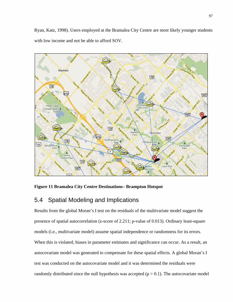
97

Ryan, Katz, 1998). Users employed at the Bramalea City Centre are most likely younger students

with low income and not be able to afford SOV.

Figure 11 Bramalea City Centre Destinations– Brampton Hotspot

5.4 Spatial Modeling and Implications Results from the global Moran’s I test on the residuals of the multivariate model suggest the

presence of spatial autocorrelation (z-score of 2.211; p-value of 0.013). Ordinary least-square

models (i.e., multivariate model) assume spatial independence or randomness for its errors.

When this is violated, biases in parameter estimates and significance can occur. As a result, an

autocovariate model was generated to compensate for these spatial effects. A global Moran’s I

test was conducted on the autocovariate model and it was determined the residuals were

randomly distributed since the null hypothesis was accepted (p > 0.1). The autocovariate model

98

corresponds to the literature that indicates a better fitted model compared to the OLS regression

model (Dormann, 2007; Augustin, 1996). The -2 log likelihood was reported to be 375.56, lower

than the multivariate model (381.33). With respect to ERH, the p-value increased slightly (from

0.134 to 0.136) to suggest any drastic changes to the modeling results. The p-value of HHI

(destination-end), however, reduced from 0.677 to 0.523, showing greater significance in the

autocovariate model but is still greater than the statistical significance threshold (p < 0.1). The

other variables in the model remained more/less the same. It is worth noting that the

autocovariate term is statistically significant (p=0.017) and has a large effect size (odds ratio of

3.528). This suggests that another process not captured in the model could have some effect on

carpool formation.

The autocovariate term represents an unknown process (i.e., not explained in the model)

that is both highly significant and has a large effect size in the regression model. It is

hypothesized that the autocovariate term could represent personal, social, and/or organizational

factors that are not controlled in the model. While regression modeling is a quantitative approach

used to explain carpool formation and usage, qualitative methods should not be disregarded as

they might assist in explaining psychological and socially influential factors (e.g., attitudes,

preferences, habits) in travel behaviour (Clifton and Handy, 2003; Poulenez-Donovan and

Ulberg, 1994). For example, in a study by Poulenez-Donovan and Ulberg (1990), a traditional

survey questionnaire was conducted to evaluate participation in an employer-based TDM

program and employee satisfaction. In addition, the employees were also interviewed about their

personal travel patterns and attitudes about the program. The findings from the interview

revealed factors that were not anticipated in the survey. For example, the interview uncovered

that many employees felt uncomfortable in the quasi-social setting of a carpool, particularly

when passengers were of a different occupational class. It stands to reason that qualitative study

99

or revision of the existing survey instrument is indicated, given the contribution of spatial effects

to the regression model.

100

6 Conclusions The thesis attempts to advance our understanding of the carpool formation and use process for

users enrolled in an employer based ride-matching program (e.g., Smart Commute’s Carpool

Zone). The sample reflects a particular group of individuals using Carpool Zone (i.e., users

enrolled in the employer-based program of Smart Commute and from the service sector) and the

study does not represent a population level study of carpooling. The primary focus of this study

is to uncover whether different built environments could affect a user’s ability to form carpools

as this topic is sparsely discussed in the literature. The research also examines the implications of

spatial autocorrelated residuals in logistic regression models and how to address this concern.

The following sections will summary the findings from this thesis (Section 6.1), provide policy

recommendations based on these findings (Section 6.2), and finally discuss future research

(Section 6.3).

6.1 Summary of Findings Objective 1: to study the role of the built environment in carpool formation in the GTHA;

The descriptive statistics presented in Section 4.1.2 reported differences between users that have

formed carpools versus those that have not. The results indicate a few key differences between

the groups with respect to the built environment. Land use mix (destination-end) was less diverse

for those who formed carpools. This suggests users are more likely to carpool when working at

monopolistic sites, such as industrial parks. The results from the carpooling hotspots analysis

support these findings as many users who had formed carpools were commuting to industrial

parks such as Sheridan Park. These sties tend to cater to mainly motorized transport and distance

between user's place of residence and their workplace tends to be at longer distances. With

regard to population density (destination-end), greater density surrounding the workplace tends

101

to work against carpooling. The literature suggest built environments that focus on creating more

job opportunities nearby the place of residences (e.g., new urbanism, complete communities)

tend to reduce motorized travel because of alternative commute options (i.e., walking and

cycling). Street density (origin-end) was found to be denser for the formed group. This would

allow greater accessibility for drivers to pick-up passengers in their carpools. Street density

(destination-end) was determined to be denser for the non-formed group. This might imply these

workplaces have greater accessibility and users are more likely to engage in sustainable transport

such as transit, walking, or cycling. Lastly, cumulative opportunities to employment (destination-

end) were greater for the non-formed group. An area with lots of job opportunities, such as a

business district, would most likely have a good transit system for workers to commute back and

forth and would make carpooling a less attractive option.

The research also used logistic regression to explain whether the built environment is a

major process in carpool formation. The results from bivariate regression reported that only the

land-use mix (destination-end) variable was significant. The model explains that as HHI

(destination-end) increases (towards homogeneity), the more likely the user would form a

carpool. This refers back to inferring land-use that is not well mixed tend to discourage

motorized travel. With respect to the multivariate and autocovariate models, both did not find the

built environment significant to suggest other variables have more importance.

Objective 2: to examine the differences and similarities between Carpool Zone users whom

have formed and not formed carpools;

In addition to the built environment differences described above (i.e., Objective 1), workplace

characteristics are statistically significant and have large differences. The results indicate that

larger firm size caters to the non-formed group. This finding, however, contradicts with the

102

literature that suggests large firm size provides greater opportunity for users to initiate in carpool

formation (Cervero and Griesenbeck, 1988; Ferguson, 1990). The number of carpool spaces was

found to be larger for those who had formed carpools. This corresponds to the literature that

suggests priority parking for carpoolers was considered important (Canning et al., 2010).

With regard to TDM programs, both ERH and flex time displayed significant differences

between the two groups. A greater number of users with flex time available at their workplace

belonged in the non-formed group. This suggests that having flex time may deter carpool

formation because of temporal irregularity of work schedules to find suitable matches. In

addition, a greater number of users with ERH available at their workplace associated with the

formed group. The findings imply the great importance for ERH in an employer-based carpool

program because it provides a safe guard to users in the case when a ride is not available due to

unforeseen circumstances. Lastly, for role preference, those who were willing to share driving

responsibilities were more apt to formed carpools than those who didn't.

Objective 3: to uncover the influence of the spatial distribution of observations (i.e., spatial

autocorrelation) on the model results;

It was determined by a Global Moran’s I test that the multivariate model exhibited spatial

autocorrelated residuals. As a result, an autocovariate regression was conducted to compensate

for this spatial effect. The finding revealed that the addition of the autocovariate term in the

regression model had little effect on parameter estimates and their significance. The

autocovariate term was significant and had a large effect size. This suggests an unknown spatial

process not captured in the model may affect the carpool formation process and would warrants

for further research to determine what this process is. It is hypothesized that psychological and

103

socially influential factors could explain this process, qualitative methods should be conducted in

future research to supplement current understandings about carpool formation and use.

Objective 4: to improve regression modeling while considering for the spatial effects (i.e.,

spatial autocorrelation).

The residuals of the ordinary logistic regression model exhibited spatial autocorrelation

which suggest that the assumption of independence or randomness was violated. The addition of

the autocovariate term in the logistic regression model reduced the deviance of the model which

suggests better model performance.

6.2 Policy Recommendations The following recommendations are provided based on the findings from this research:

• The promotion of the Emergency Ride Home (ERH) program to potential carpoolers is

an important recommendation to Smart Commute. ERH programs provides commuters

who regularly use a sustainable mode of transport to work (e.g., vanpool, carpool, bike,

walk, transit) with a reliable ride home in the event of unexpected emergencies in the

form of cab fare, rental car, bus/train expenses. The results revealed a substantial

proportion of people engaging in carpooling that also have ERH available at their

workplace.

• The research recommends Smart Commute to target monopolistic workplaces (less

diverse land use mix). The results suggest users working at these locations (e.g.,

industrial parks) are more likely to carpool. These locations are catered for motorized

transport (i.e., SOV and carpooling) because they are located nearby major

104

roads/highways. In addition, these workplaces tend to be located in the suburbs/exurban

areas where public transit might be limited and hard to access.

• It is recommended that the number of carpool spaces at the workplace should be

increased. The results from the study suggest users who formed carpools had a greater

number of carpool spaces at their workplace than those who did not formed carpools.

Canning et al. (2010) found users enrolled in employer-based carpool programs to rate

priority parking very highly. Priority parking refers to reserved parking spots nearby the

building that are more desirable.

6.3 Future Research With regard to future research, a longitudinal study (i.e., repeated observation of the same

variables over long periods of time) on the carpool formation process would be beneficial to the

researcher. It would capture the entire process from enrollment to the point of starting and using

a carpool. A longitudinal study would allow researchers to observe how long users can maintain

a successful carpool and determine whether carpooling is a short term or long term process. In

addition, this sort of study would let researchers examine the registration process more carefully.

Some potential research questions include: how long did it take to form a carpool upon

registration? What were the difficulties to form carpool during this process?

105

References Al-Kazily, J., Barnes, C., Coontz, N. (1994). Household Structure and Travel Behavior. NPTS Demographic Special Reports. Washington, D.C. Federal Highway Administration.

Anselin, L. (1994). Local Indicators of Spatial Association - LISA. Geographic Analysis. 27(2), 25p.

Augustin, N., Mugglestone M., Buckland S. (1996). An Autologistic Model for the Spatial Distribution of Wildlife. Journal of Applied Ecology. 33(2),339-347.

Baldassare, M., Ryan, S,. & Katz, C. (1998). Suburban attitudes toward policies aimed at reducing solo driving. Transportation, 25, 99-117.

Benkler, Y. (2004). Sharing Nicely. On shareable goods and the emergence of sharing as a modality of economic production. Yale Law Review, 114, 273- 358.

Black, A. (1995). Urban Mass Transportation Planning. McGraw Hill, 411 pp.

Blumenberg, E., Smart, M. (2010). Getting by with a little help from my friends...and family: immigrants and carpooling. Transportation, 37,429-446.

Boarnet, M., Crane, R. (2001). Travel by Design – The Influence of Urban Form on Travel. Oxford University Press.

Boslaugh, S. (2007). Secondary Data Sources for Public Health. Cambridge University Press.

Brownstone, D., and Golob, F. (1992). The effectiveness of ridesharing incentives: Discrete- choice models of commuting in Southern California. Regional Science and Urban Economics, 22, 5-24.

Brunso J.M., Hartgen D.T. (1981). Can employer-based carpool coordinators increase ridesharing? Transportation Research Record, 823:45-50.

Buliung, R., Soltys, K., Bui, R., Habel, C., Lanyon, R. (2010). Catching a Ride on the Information Super-Highway: Toward an Understanding of Internet-based Carpool Formation and Use. Transportation, 37(6), 849-873.

Camstra, R. (1996). Commuting and Gender in a Lifestyle Perspective. Urban Studies, 33, 283-300.

Canning, P.E., Hughes, S.J., Hellawell, E.E., Gatersleben, B.C.M. and Fairhead, C.J. (2010). Reasons for participating in formal employer-led carpool schemes as perceived by their users. Transportation Planning and Technology, 33(8), 733 — 745.

106

Cervero, R. and Murakami, J. (2010). Effects of Built Environments on Vehicle Miles Traveled: Evidence from 370 U.S. Urbanized Areas. Environment and Planning A, 42(2), 400-418.

Cervero, R., & Griesenbeck, B. (1988). Factors influencing commuting choices in suburban labor markets: a case analysis of Pleasanton, California. Transportation Research Part A, 22A (3), 151-161.

Cervero, R., Kockelman, K. (1997). Travel demand and the 3Ds: Density, diversity, and design. Transportation Research Part D: Transport and Environment, 2(3), 99-219.

Charles, K.K., Kline, P. (2006). Relational Costs and the Production of Social Capital: Evidence from Carpooling. The Economic Journal, 116(511), 581-604.

Cline, M., Sparks C., Eschbach, K. (2009). Understanding Carpool Use by Hispanics in Texas. Transportation Research Record, No.2118, 39-46.

Collura, J. (1994). Evaluating ride-sharing programs: Massachusetts’ experience. Journalof Urban Planning & Development, 120(1), 28-47.

Commuter Connections. (2011). Why Carpool? - Carpooling Advantages. Retrieved August 15, 2011 from http://www.mwcog.org/commuter2/commuter/ridesharing/whycarpool.html

Concas, S., Winters, P. (2010). Impact of Carpooling on Trip-Chaining Behavior and Emission Reductions. Transportation Research Record, No. 2010, 83-91.

Correia, G., Viegas, J. (2011). Carpooling and carpool clubs: Clarifying concepts and assessing value enhancement possibilities through a Stated Preference web survey in Lisbon, Portugal. Transportation Research Part A, 45, pp.81-90.

Dailey, D.J., & Meyers, D. (1999). Seattle Smart Traveller: Dynamic Rides Matching on the World Wide Web. Transportation Research part C, 7, 17-32.

Dargay, J., & Hanly, M. (2007). Volatility of car ownership, commuting mode and time in the UK. Transportation Research Part A: Policy and Practice, 41(10), 934-948.

Data Management Group. (2009). 2006, 2001, 1996 and 1986 Travel Survey Summaries for the Greater Toronto and Hamilton Area. Retrieved August 15, 2011 from http://www.dmg.utoronto.ca/pdf/tts/2006/travel_summaries_for_the_gtha/TTS_Report5_ full.pdf

Dill, J. (2005). Measuring Network Connectivity for Bicycling and Walking, School of Urban Studies and Planning, Portland State University. Transportation Research Board 2004 Annual Meeting.

Dormann, C. (2007). Assessing the validity of autologistic regression. Ecological Modelling. 207(2-4), 234-242.

107

Environment Canada. (2007). Greenhouse Gas Division. National Inventory Report 1990- 2005: Greenhouse Gas Sources and Sinks in Canada. Ottawa, Environment Canada, 2007 (Cat. No. En81-4/2005E, Table 3-4).

Ewing, R. and Cervero, R. (2010). Travel and the Built Environment. Journal of the American Planning Association, 76(3), 265-294.

Ewing, R., and R. Cervero. (2001). Travel and the Built Environment: A Synthesis. Transportation Research Record, 1780, 87-114.

Federal Highway Administration. (2007). Highway Statistics 2007. Retrieved August 15, 2011 from http://www.fhwa.dot.gov/policyinformation/statistics/2007/

Ferguson, E. (1995). The Demographics of Carpooling. Transportation Research Record,1496, 142-150.

Ferguson, E. (1997). The rise and fall of the American carpool: 1970-1990. Transportation, (24)4, 349-376.

Frej, A. (2001). Business Park and Industrial Development Handbook; 2nd edition. New York: Urban Land Institute.

Gard, J. (2007). Innovative Intermodal Solutions for Urban Transportation Paper Award: Quantifying Transit-Oriented Development's Ability To Change Travel Behavior. ITE Journal. 77(11), 42-46.

Habib, K.M.N., Tian, Y., Zaman, H. (2011). Modelling Carpool Mode Choice with Explicit Consideration of Willingness to Consider Carpool in Choice Set by Hybrid Choice Model. Transportation 38(4), 587-604.

Handy S L, & Niemeier, D A,. (1997). Measuring accessibility: an exploration of issues and alternatives, Environment and Planning A, 29(7), 1175 – 1194.

Handy, S., Paterson, R.G., Butler, K. (2004). Planning for Street Connectivity: Getting From Here to There, Planning Advisory Service Report 515, American Planning Association.

Hemson Consulting, Ltd. (2005). The Growth Outlook for the Greater Golden Horseshoe. Retrieved August 15, 2011 from http://www.hemson.com/downloads/GrowthOutlookForGGH%2017Jan2005a.pdf.

Horowitz, A., Sheth, J. (1978). Ridesharing to work: an attitudinal analysis. Transportation Research Record, 637, 1–8.

HowToStartACarpool.com. (2011). Carpool History. Retrieved August 15, 2011 from http://www.howtostartacarpool.com/carpool_history.php.

Hwang, K., Giuliano, G. (1990). The determinants of ridesharing: literarture review. Working Paper No. 38, University of California, Berkeley: University of California Transportation Center.

108

Industry Canada. (2009). Canadian Industry Statistics. Retrieved August 15, 2011 from http://www.ic.gc.ca/eic/site/cis-sic.nsf/eng/Home

INRIX. (2010). National Traffic Scorecard. Retrieved August 15, 2011 from http://scorecard.inrix.com/scorecard/.

Jacobson, S., King D. (2009). Fuel saving and ridesharing in the US: Motivations, limitations, and opportunities. Transportation Research Part D, 14, 14-21.

Jakobsson, C., Fujii, S., Garling, T. (2000). Determinants of private car users’ acceptance of road pricing. Transport Policy 7, 153-158.

Kaufman, S. (2002). Why people (don’t) carpool and change for the better: A social capital framework for investigating environmental behaviour. Conference paper based on honours research, presented at the 2nd National Conference of Sustainable Campuses, RMIT, Melbourne, 2002.

Koppelman, F., Bhat, C., Schofer, J. (1993). Market Research Evaluation of Actions to Reduce Suburban Traffic Congestion: Commuter Travel Behavior and Response to Demand Reduction Actions. Transportation Research Part A, 27A, 383-393.

Kuzmyak, J.R., Pratt, R.H., Douglas, G.B., Spielberg, F. (2003). Land Use and Site Design - Traveler Response to Transportation System Changes. Transit Cooperative Research Program (TCRP) Report 95: Chapter 15, published by Transportation Research Board, Washington.

Levin, I. (1982). Measuring Tradeoffs in Carpool Driving Arrangement Preferences. Transportation (pre-1986), 11(1), 71-85.

Lue, A., Colorni, A. (2009). A software tool for commute carpooling: a case study on university students in Milan. International Journal of Services Sciences. 2, 222-241.

McGuckin, N., Zmud, J., Nakamoto, Y. (2005). Trip-Chaining Trends in the United States: Understanding Travel Behavior for Policy Making. Transportation Research Record, No. 1917, 199-204.

McMillan J., Hunt J. (1997). A Stated Preference Investigation of Commuter's Attitudes Towards Carpooling in Calgary. Transportation Research Record. Vol. 1598, 9-17.

Metrolinx. (2011a). Metrolinx Overview. Retrieved August 15, 2011 from http://www.metrolinx.com/en/aboutus/metrolinxoverview/metrolinx_overview.aspx

Metrolinx. (2011a). The Big Move – Introduction. Retrieved August 15, 2011 from http://www.metrolinx.com/thebigmove/en/introduction/.

Meyer, M. (1999). Demand management as an element of transportation policy: using carrots and sticks to influence travel behaviour. Transportation Research Part A,33(7), 575-599.

109

Ministry of Public Infrastructure Renewal (MPIR). (2006). Growth Plan for the Greater Golden Horseshoe 2006. Retrieved August 15, 2011 from https://www.placestogrow.ca/images/pdfs/FPLAN-ENG-WEB-ALL.pdf.

Modarres, A. (1993). Evaluating employer-based transportation demand management programs. Transportation Research Part A, 27(4), 291-297.

Morency, C. (2007). The ambivalence of ridesharing. Transportation, 34(2), 239-253.

National Energy Board. (2009). Canadian Energy Demand: Passenger Transportation - Energy Briefing Note. Retrieved August 15, 2011 from http://www.neb.gc.ca/clf- nsi/rnrgynfmtn/nrgyrprt/nrgdmnd/pssngrtrnsprttn2009/pssngrtrnsprttn-eng.html

Ontario Chamber of Commerce. (2004). Cost of Border Delays to Ontario Report. Retrieved August 15, 2011 from http://occ.on.ca/2004/05/cost-of-border-delays-to-ontario-report/.

Ontario Ministry of Energy. (2011). Oil and Gas : Fuel Prices. Ontario Ministry of Energy and Infrastructure. http://www.mei.gov.on.ca/en/energy/oilandgas/?page=fuel-prices.

Orford, S. (2004). Identifying and comparing changes in the spatial concentrations of urban poverty and affluence: a case study of inner London. Computers, Environment and Urban Systems. 28(6),701-717.

Organization for Economic Cooperation and Development (OECD). (2010). OECD Territorial Reviews: Toronto, Canada. Retrieved August 15, 2011 from http://www.oecd.org/document/1/0,3343,en_2649_34413_43985281_1_1_1_1,00.html#k eyfacts.

Peduzzi, P., Concato, J., Kemper E., Holford, T.R. and Feinstein, A.R. (1996). A simulation study of the number of events per variable in logistic regression analysis. Journal of Clinical Epidemiology, 49, 1372-1379.

PickupPal. (2009). Save PickupPal in Ontario. Retrieved August 15, 2011 from http://save.pickuppal.com/.

Pisarski, A. (2006). Commuting in America III, The Third National Report on Commuting Patterns and Trends. Transportation Research Board Report, Washington, D.C.

Polena, C., Glazer, L. (1991). An examination of eleven guaranteed-ride-home programs nationwide, presented at Annual Meeting of Transportation Research Board, Washington, DC, Jan. 13-17.

Poulenez-Donovan, C.J., Ulberg, C. (1994). Seeing the trees and missing the forest: qualitative versus quantitative research findings in a model transportation demand management program evaluation. Transportation Research Record. 1459, 1-6.

Public Vehicles Act. (2009). Retrieved August 15, 2011 from http://www.e- laws.gov.on.ca/html/statutes/english/elaws_statutes_90p54_e.htm.

110

R Development Core Team (2011). R: A language and environment for statistical computing. R Foundation for Statistical Computing, Vienna, Austria. ISBN 3-900051-07-0, URL http://www.R-project.org.

Sermons, M.W. and Koppelman, F.S. (2001) Representing the differences between female and male commute behavior in residential location choice models, Journal of Transport Geography, 9, 101-110.

Slug-Lines.com. (2009). About Slugging. Retrieved August 15, 2011 from http://slug- lines.com/Slugging/About_slugging.asp.

Southworth, M., Ben-Joseph, E. (2003). Streets and the shaping of towns and cities. Island Press.

Statistics Canada. (2007a). Table 4050004 - Road motor vehicles, registrations, annually (Number). Statistics Canada.

Statistics Canada. (2008a). Text Table 3.14 - Households that owned or leased a motor vehicle and distance travelled in an average year, by province, 2006. Retrieved August 15, 2011 from http://www.statcan.gc.ca/pub/11-526-x/2007001/t/5213678-eng.htm.

Statistics Canada. (2008b). Commuting Patterns and Places of Work of Canadians, 2006 Census: National, provincial and territorial portraits. Retrieved August 15, 2011 from http://www.statcan.gc.ca/bsolc/olc-cel/olc-cel?catno=97-561- XIE2006001&lang=eng&issnote=1.

Statistics Canada. (2008c). Census of Canada, 2006: income and earnings for census metropolitan areas, tracted census agglomerations and census tracts [computer file]. Ottawa, Ont.: Statistics Canada [producer and distributor], 2008/04/16 (Topic-based tabulations; 97-563-xcb2006052) <http://www.chass.utoronto.ca/datalib/cc06/tbt06.htm#97-563>

Statistics Canada. (2009). Employed labour force(1) by mode of transportation, both sexes, 2006 counts, for Canada, provinces and territories of residence - 20% sample data. 2006 Census: Data products. Retrieved August 15, 2011 from http://www12.statcan.ca/census- recensement/2006/dp-pd/hlt/97-561/T603- eng.cfm?Lang=E&T=603&GH=4&SC=1&SO=99&O=A

Strathman, J., K. Dueker and J. Davis. (1994). Effects of Household Structure and Selected Travel Characteristics on Trip Chaining. Transportation, 21, 23-45.

Taaffe, E., Gauthier, H., O'Kelly, M. (1996). Geography of Transportation. New Jersey: Prentice Hall College Div.

Teal, R. (1987). Carpooling: Who, How and Why. Transportation Research, 21A(3), 203- 214.

111

Tischer, M., & Dobson, R. (1979). An Empirical Analysis of Behavioural Intentions of Single-Occupant Auto Drivers to Shift to High Occupancy Vehicles. Transportation Research, 13A(3), 143-158.

Tobler, W. (1970). A computer movie simulating urban growth in the Detroit region. Economic Geography, 46(2), 234-240.

Toronto Board of Trade. (2011). Scorecard on Prosperity 2011 – Toronto Region Moves to Number Eight from Fourth. Retrieved August 15, 2011 from http://www.bot.com/AM/Template.cfm?Section=Scorecard&Template=/CM/HTMLDisp lay.cfm&ContentID=3418.

Tsao, H.S., & Lin, D-J. (1999). Spatial and Temporal Factors in Estimating the Potential of Ride-sharing for Demand Reduction. Institute of Transportation Studies, 1999.

Turcotte, M. (2008). The difference between city and suburb: How can we measure it? Canadian Social Trends, 85. Catalogue no. 11-008-XIE, Ottawa: Minister of Industry.

Van Vugt, M., Van Lange, P.A.M., Meertens, R.M. & Joireman, J.A. (1996). How a structural solution to social dilemma failed: A field experiment on the first carpool lane in Europe. Social Psychology Quarterly, 59, 364-374.

VIARail. (2009). Overview Via Rail. Retrieved August 15, 2011 from http://www.viarail.ca/en/about-via-rail.

Washbrook, K., Haider, W., & Jaccard, M. (2006). Estimating commuter mode choice: A discrete choice analysis of the impact of road pricing and parking charges. Transportation, 33(6), 621-639.