1

Total Variation Regularized Tensor RPCA forBackground Subtraction from Compressive

MeasurementsWenfei Cao, Yao Wang, Jian Sun, Member, IEEE, Deyu Meng, Member, IEEE, Can Yang,

Andrzej Cichocki, Fellow, IEEE and Zongben Xu

Abstract—Background subtraction has been a fundamentaland widely studied task in video analysis, with a wide rangeof applications in video surveillance, teleconferencing and 3Dmodeling. Recently, motivated by compressive imaging, back-ground subtraction from compressive measurements (BSCM)is becoming an active research task in video surveillance. Inthis paper, we propose a novel tensor-based robust PCA (Ten-RPCA) approach for BSCM by decomposing video frames intobackgrounds with spatial-temporal correlations and foregroundswith spatio-temporal continuity in a tensor framework. In thisapproach, we use 3D total variation (TV) to enhance the spatio-temporal continuity of foregrounds, and Tucker decompositionto model the spatio-temporal correlations of video background.Based on this idea, we design a basic tensor RPCA model overthe video frames, dubbed as the holistic TenRPCA model (H-TenRPCA). To characterize the correlations among the groupsof similar 3D patches of video background, we further design apatch-group-based tensor RPCA model (PG-TenRPCA) by jointtensor Tucker decompositions of 3D patch groups for modelingthe video background. Efficient algorithms using alternatingdirection method of multipliers (ADMM) are developed to solvethe proposed models. Extensive experiments on simulated andreal-world videos demonstrate the superiority of the proposedapproaches over the existing state-of-the-art approaches.

Index Terms—Background subtraction, compressive imaging,video surveillance, robust principal component analysis, tensordecomposition, 3D total variation, nonlocal self-similarity.

This work was supported in part by the Major State Basic ResearchProgram under grant number 2013CB329404; in part by the Natural ScienceFoundation of China under grant numbers 11501440, 61273020, 61373114,61472313, 61501389 and 61573270; in part by the Hong Kong Research GrantCouncil under grant number 22302815, and the grant FRG2/15-16/011 fromHong Kong Baptist University. (Corresponding author: Yao Wang.)

W. Cao is with the School of Mathematics and Statistics, Xi’an JiaotongUniversity, Xi’an 710049, China, and also with the School of Mathematicsand Information Science, Shaanxi Normal University, Xi’an 710119, China(e-mail: caowenf2015@gmail.com).

Y. Wang is with the School of Mathematics and Statistics, Xi’an JiaotongUniversity, Xi’an 710049, China, and also with the Shenyang Institute ofAutomation, Chinese Academy of Sciences, Shenyang 110016, China (e-mail:yao.s.wang@gmail.com).

J. Sun, D. Meng and Z. Xu are with the School of Mathematics andStatistics, Xi’an Jiaotong University, Xi’an 710049, China (e-mail: jiansun,dymeng, zbxu@mail.xjtu.edu.cn).

C. Yang is with the Department of Mathematics, Hong Kong BaptistUniversity, Kowloon, Hong Kong (e-mail: eeyang@hkbu.edu.cn).

A. Cichocki is with the RIKEN BSI, Wako-shi 351-0198, Japan, and alsowith the Systems Research Institute, PAS, Warsaw 01-447, Poland, and withthe Skolkovo Institute of Science and Technology (SKOLTECH), Moscow143025, Russia (e-mail: a.cichocki@riken.jp).

I. INTRODUCTION

Since 1990s, background subtraction [1]–[6] has been at-tracting great attention in the fields of image processing andcomputer vision. It aims at simultaneously separating videobackground and extracting the moving objects from a videostream, which provides important cues for numerous applica-tions such as moving object detection [7], object tracking insurveillance [8], etc.

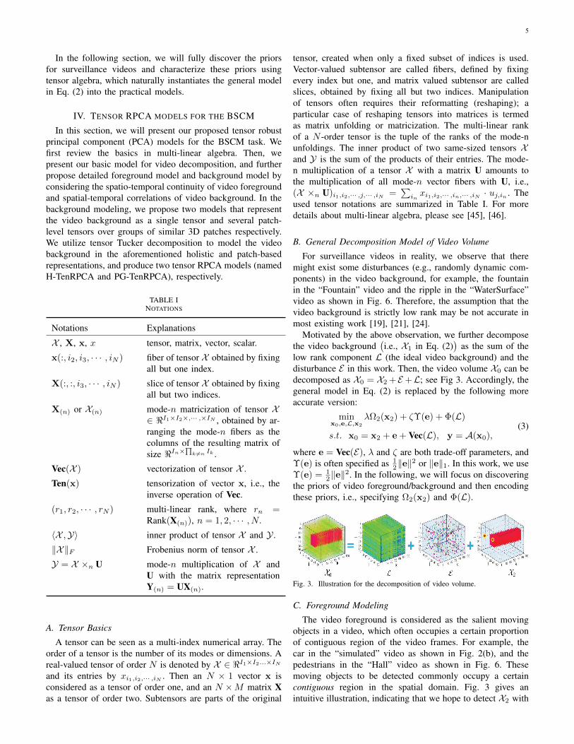
Most of the current video background subtraction tech-niques consist of four steps: video acquisition, encoding,decoding, and separating the moving objects from back-ground [1]. For example, Lamarre and Clark [9] performedbackground subtraction on JPEG encoded video frames using aprobabilistic model; Aggarwal et al. [10] considered detectingmoving objects on a MPEG-compressed video using DCTcoefficients of video frames. These conventional approachescommonly implement video acquisition, coding, and back-ground subtraction in separate procedures. This conventionalscheme requires to fully sample the video frames with largestorage requirements, followed by well-designed video codingand background subtraction algorithms. Recently, motivatedby compressive sensing (CS) [11]–[13] in signal process-ing, we focus on a newly-developed compressive imagingscheme [14]–[17] for background subtraction by combiningthe video acquisition, coding and background subtraction intoa single framework, which is called background subtrac-tion from compressive measurements (BSCM). Figure 1shows an illustrative example. The video imaging systemfirst captures compressive measurements from the scenes, andthen transmits these measurements to the processing centerfor foreground/background reconstruction. Compared to theconventional scheme, this new scheme need not fully sense allthe video voxels, and thus heavily reduces the computationaland storage costs and even the energy consumption of imagingsensors.

The task of the BSCM is to reconstruct the original videowith high fidelity and meanwhile accurately separate themoving objects from video background based on compressivemeasurements. The objective on this task is to maximizethe reconstruction and separation accuracies using as fewcompressive measurements as possible. This is a heavily ill-posed inverse problem and it is necessary to discover thevideo prior knowledge to make this problem well-posed. Therealready exist some works [18]–[22] on the task of the BSCM.

arX

iv:1

503.

0186

8v4

[cs

.CV

] 5

Jun

201

6

2

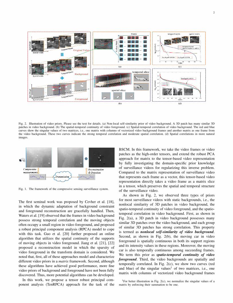
Fig. 2. Illustration of video priors. Please see the text for details. (a) Non-local self-similarity prior of video background. A 3D patch has many similar 3Dpatches in video background. (b) The spatial-temporal continuity of video foreground. (c) Spatial-temporal correlation of video background. The red and bluecurves show the singular values of two matrices, i.e., one matrix with columns of vectorized video background frames and another matrix as one frame fromthe video background. These two curves indicate the strong temporal correlation and moderate spatial correlation. (d) Spatial correlations in more naturalimages.

Fig. 1. The framework of the compressive sensing surveillance system.

The first seminal work was proposed by Cevher et al. [18],in which the dynamic adaptation of background constraintand foreground reconstruction are gracefully handled. Then,Waters et al. [19] observed that the frames in video backgroundpossess strong temporal correlation and the moving objectsoften occupy a small region in video foreground, and proposeda robust principal component analysis (RPCA) model to copewith this task. Guo et al. [20] further proposed an onlinealgorithm that utilizes the spatial continuity of the supportsof moving objects in video foreground. Jiang et al. [21], [22]proposed a reconstruction model in which the sparsity ofvideo foreground in the transform domain is considered. Wenoted that, first, all of these approaches model and characterizedifferent video priors in a matrix framework. Second, althoughthese algorithms have achieved good performance, more finevideo priors of background and foreground have not been fullydiscovered. Thus, more potential algorithms can be developed.

In this work, we propose a tensor robust principal com-ponent analysis (TenRPCA) approach for the task of the

BSCM. In this framework, we take the video frames or videopatches as the high-order tensors, and extend the robust PCAapproach for matrix to the tensor-based video representationby fully investigating the domain-specific prior knowledgeof surveillance videos for regularizing this inverse problem.Compared to the matrix representation of surveillance videothat represents each frame as a vector, this tensor-based videorepresentation directly takes a video frame as a matrix slicein a tensor, which preserves the spatial and temporal structureof the surveillance video.

As shown in Fig. 2, we observed three types of priorsfor most surveillance videos with static backgrounds, i.e., thenonlocal similarity of 3D patches in video background, thespatio-temporal continuity of video foreground, and the spatio-temporal correlation in video background. First, as shown inFig. 2(a), a 3D patch in video background possesses manysimilar 3D patches over the video background, and each groupof similar 3D patches has strong correlation. This propertyis termed as nonlocal self-similarity of video background.Second, as shown in Fig. 2(b), the moving car in videoforeground is spatially continuous in both its support regionsand its intensity values in these regions. Moreover, the movingcar is also temporally continuous among succeeding frames.We term this prior as spatio-temporal continuity of videoforeground. Third, the video backgrounds are spatially andtemporally correlated. In Fig. 2(c), we show two curves (redand blue) of the singular values1 of two matrices, i.e., onematrix with columns of vectorized video background frames

1For better illustration in Fig. 2(c), we normalize the singular values of amatrix by enforcing their summation to be one.

3

and another matrix as one frame from the video background.The drastically decaying trend of the red curve indicatesthe strong temporal correlation among the video backgroundframes and the slow decaying trend of the blue curve indicatesthe weak correlation in the spatial domain. Let us define theaccumulation energy ratio of top k normalized singular valuesas AccEgyR =

∑i nsvi, where nsvi is the i-th normalized

singular value, i.e., nsvi = svi/∑i svi and svi is the i-th

singular value. The arrow box for the red curve indicates thatonly top 3 singular values can attain the ratio 0.9030 whilethe arrow box for the blue curve indicates that top 84 singularvalues can attain the ratio 0.9770. These quantitative valuesjustify that the video background has strong correlation amongits frames and each video background frame has weak spatialcorrelation. Fig. 2(d) further exhibits the weak correlationsin other natural images. We term this observation as spatio-temporal correlation of video background.

Based on the aforementioned video priors, we model theBSCM in a tensor RPCA framework (TenRPCA) using Tuckerdecomposition technique. With our model, a video volumerepresented by a tensor is decomposed into a backgroundlayer based on its spatial-temporal correlation and foregroundlayer based on its spatial-temporal continuity. We design aTucker decomposition approach to model the spatio-temporalcorrelation in video background and a 3D total variation(TV) term to enforce the spatio-temporal continuity of videoforeground. Along this idea, we propose two TenRPCA modelsby representing video background as a single tensor and a fewpatch-level tensors over groups of similar 3D patches, whichare dubbed as holistic tensor RPCA model (H-TenRPCA)and patch-group-based tensor RPCA model (PG-TenRPCA)respectively. We design efficient algorithms using the alter-nating direction method of multipliers (ADMM) to optimizethese proposed models. The experiments on synthetic and realvideos demonstrate that our proposed two TenRPCA modelsachieve higher reconstruction and background/foreground sep-aration accuracies with fewer compressive measurements thanthe existing state-of-the-art approaches. Moreover, the PG-TenRPCA model generally works better than the H-TenRPCAmodel which indicates the effectiveness of our modeling ofthe nonlocal self-similarity of video background.

Our contributions can be summarized as four folds: First,to the best of our knowledge, we are the first to model theBSCM task in a tensor robust PCA framework. Compared tothe matrix-based video representation, this tensor-based videorepresentation well preserves the spatial-temporal structuresof video, which enables us to fully characterize the priors ofvideo spatial-temporal structures in our framework. Second,we fully investigate the video priors for the BSCM task. Wedesign a 3D total variation (TV) term to encode the spatio-temporal continuity of video foreground, and a Tucker decom-position approach to model the spatio-temporal correlation ofvideo background. Third, based on the observation of nonlocalself-similarity of video background, we design a patch-levelbackground model using joint Tucker decomposition overgroups of similar 3D patches to model the strong correlationsamong similar 3D patches. This model significantly outper-forms our holistic TenRPCA model which represents the video

background as a single tensor. Finally, based on ADMM withthe adaptive scheme, we design efficient algorithms to solvethe proposed models, and achieve superior performance overthe existing methods on various video data sets, especiallywhen the sampling ratio is very low.

The remaining of this paper is organized as follows. InSection II, the related works will be discussed. In Section III,the general framework of the BSCM will be reviewed. Ourmodels and their motivations will be presented in Section IV.In Section V, efficient algorithms will be designed to solvethe proposed models. In Section VI, extensive experimentson various surveillance video data sets will be conducted tosubstantiate the superiority of the proposed models over theother existing ones. This paper will be concluded with somediscussions on future work in Section VII.

II. RELATED WORK

A. Background Subtraction without Compressive Imaging

Various approaches for background subtraction using con-ventional imaging cameras have been developed since 1990sand obtained a wide range of applications in many fields.These approaches can be mainly categorized into the followingfive classes: the basic approach, the statistical approach, thefuzzy approach, the neural and neuro-fuzzy approach, and thesubspace learning approach [1]–[6].

Among these traditional approaches, the subspace learningapproach has been attracting wide attentions in the field ofmachine learning and computer vision. One classical work onthis task was proposed by Oliver et al. [23], which uses aneigenspace (PCA) idea to model the background. Aiming atremedying the outlier and heavy noise issue, Candes et al. [24]proposed robust principal component analysis (RPCA) to resistthe gross sparse noise. This seminal work has triggered atremendous interest in dealing with background subtractionusing different formulations of RPCA. For example, theMarkov random field (MRF) regularized RPCA technique wasproposed in Zhou et al. [25], a novel block sparse RPCAformulation was proposed in [26], total variation regularizedRPCA and matrix factorization methods were respectivelyproposed in Cao et al. [27] and Guo et al. [28], and the prob-abilistic versions of RPCA were proposed in Ding et al. [29]and Babacan et al. [30], respectively. In the recent work, Zhaoet al. [31] proposed a new probabilistic variant by extractingmulti-layer structures with certain physical meanings using themixture of Gaussians (MOG).

To meet the real-time requirements in practical applications,various online subspace learning approaches were developed.Rymel et al. [32] and Li et al. [33] respectively proposedan incremental PCA method to handle the newly comingvideo streams. By constraining the subspace on Grassmannianmanifold, Balzano et al. [34]–[37] proposed two efficientapproaches named GROUSE and GRASTA respectively, todeal with online subspace identification and tracking (SIT)task. Additionally, it was reported that the proposed GROUSEand GRASTA can effectively achieve the real-time backgroundsubtraction through sampling the voxels of video sequence. Xuet al. [38] further proposed an updated version of GRASTA

4

by modeling the contiguous structure of supports of videoforeground using group sparsity. Chi et al. [39] developedan online parallel SIT algorithm using recursive least squarestechnique for real-time background subtraction.

B. Background Subtraction with Compressive Imaging

Recently, multiple studies have been carried out for thebackground subtraction problem from the perspective of com-pressive imaging, in which it is required to simultaneouslyperform background subtraction and video reconstruction. Thefirst seminal work was considered by Cevher et al. [18], inwhich the dynamic adaptation of background constraint andforeground reconstruction are gracefully handled. Recently,based on the theoretical results of `1-`1 minimization [40],Mota et al. [41] proposed an efficient adaptive-rate algorithmto deal with the BSCM task. Additionally, a series of workhave been proposed based on the matrix RPCA technique.Waters et al. [19] integrated the matrix RPCA methodologyinto the framework of the BSCM and then developed a greedyalgorithm called SpaRCS to solve the resulting model. Guo etal. [20] developed an online RPCA algorithm that models thespatial continuity prior of moving objects in the foreground.Jiang et al. [21], [22] proposed a new RPCA model in whichthe sparsity of video foreground in the transform domain isconsidered based on certain practical requirements.

The matrix RPCA approaches for the BSCM commonlymodel the video as a matrix with columns of vectorizedvideo frames. Although the matrix RPCA methodology hasbeen an increasingly useful technique, it fails in fully ex-ploiting the prior knowledge on the intrinsic structures ofvideo after vectorizing the video frames. Our proposed tensorRPCA approach considers more extensive spatio-temporalprior knowledge of video background and foreground usingtensor representation of video. Such full utilization of priorinformation makes our approach capable of achieving a bettervideo reconstruction quality and simultaneously detecting themoving objects in foreground from a limited number ofcompressive measurements, as will be shown in Section VI.We also noted that the tensor compressive sensing modelswere recently proposed in [42], [43]. But they are significantlydifferent from our models, because these model are designedfor the image/video compressive sensing task instead of themore complex BSCM task considered in this paper.

III. THE GENERAL FRAMEWORK OF THE BSCMIn this section, we will present the general framework

for the BSCM task. We will mainly focus on the mathe-matical modeling and algorithm design in the pipeline ofBSCM, i.e., reconstruct video foreground and backgroundfrom compressive measurements. In the followings, we willintroduce the basic components of the BSCM task, includingthe representation of video volume, compressive operator, andvideo reconstruction and separation.

A. Video Volume

Video frames within a short period are collected as avideo volume. If the video frame has a single channel, then

the video volume can be represented as a 3-order tensorX0 := X1

0,X20, ...,X

D0 , where each matrix Xi0 ∈ <H×W (i =

1, 2, · · · , D) represents i-th frame. H and W denote the heightand width of a frame and D denotes the number of frames.This tensor has 3 modes including height, width and time. Weassume that the video volume to be reconstructed can be sepa-rated into a static component (video background) X1, and a dy-namic component (video foreground) X2, i.e., X0 := X1 +X2,where X1 := X1

1,X21 · · · ,XD1 and X2 := X1

2,X22 · · · ,XD2 .

In the following, we denote the vectorization of a videovolume X0 by x0 := [x10; x20; · · · , xD0 ], and the vectorization ofvideo background and foreground by x1 := [x11; x2

1; · · · , xD1 ]and x2 := [x12; x22; · · · , xD2 ], respectively.

B. Compressive Operator

Compressive operator can be considered as the effectiveencoding of video volume. Currently, how to design a highquality compressive operator is a crucial research topic inthe CS community; see [47]. For video data, the compressivemeasurements y can be obtained by

y = A(x0), (1)

where y is a vector of length M , and A indicates a givencompressive operator.

In this work, the randomly permuted Walsh-Hadamard op-erator [21] and the randomly permuted noiselet operator [44]will be employed as compressive operators because of theirlow computational cost and easy hardware implementation.Compressive operator can be instantiated as A = D ·H · P,where P is a random permutation matrix, H is the Walsh-Hadamard transform or the noiselet transform, and D is a ran-domly down sampling operator. As stated in [15], compressiveoperator often encodes video volume X0 through two ways.One is the holistic manner, i.e., y= D·H·P(x0), which directlycollects full 3D measurements of a video sequence. The otheris the frame-wise manner, i.e., yd= Dd · Hd · Pd(xd0) (d =1, 2, · · · , D), which collects 2D frame-by-frame measurementsyd and then concatenates all yd into a long vector y. In mostexperiments of this work, compressive operator A will be setas the frame-by-frame one.

C. Reconstruction and Separation of Video Volume

As we know, recovering X0 and simultaneously separatingX1 with X2 from the compressive measurements y is a heavilyill-posed inverse problem. Hence, it is necessary to regularizethis inverse problem by discovering the underlying video priorknowledge. Mathematically, the regularized inverse problemcan be generally formulated as

minx0,x1,x2

λΩ2(x2) + Ω1(x1)

s.t. x0 = x2 + x1, y = A(x0),(2)

where Ω1(x1) and Ω2(x2) are the prior knowledge modelingterms on video background and foreground, respectively;x0, x1 and x2 are the vectorizations of X0, X1 and X2,respectively; and λ is a trade-off parameter between the termsΩ1(x1) and Ω2(x2).

5

In the following section, we will fully discover the priorsfor surveillance videos and characterize these priors usingtensor algebra, which naturally instantiates the general modelin Eq. (2) into the practical models.

IV. TENSOR RPCA MODELS FOR THE BSCM

In this section, we will present our proposed tensor robustprincipal component (PCA) models for the BSCM task. Wefirst review the basics in multi-linear algebra. Then, wepresent our basic model for video decomposition, and furtherpropose detailed foreground model and background model byconsidering the spatio-temporal continuity of video foregroundand spatial-temporal correlations of video background. In thebackground modeling, we propose two models that representthe video background as a single tensor and several patch-level tensors over groups of similar 3D patches respectively.We utilize tensor Tucker decomposition to model the videobackground in the aforementioned holistic and patch-basedrepresentations, and produce two tensor RPCA models (namedH-TenRPCA and PG-TenRPCA), respectively.

TABLE INOTATIONS

Notations Explanations

X , X, x, x tensor, matrix, vector, scalar.

x(:, i2, i3, · · · , iN ) fiber of tensor X obtained by fixingall but one index.

X(:, :, i3, · · · , iN ) slice of tensor X obtained by fixingall but two indices.

X(n) or X(n) mode-n matricization of tensor X∈ <I1×I2×,··· ,×IN , obtained by ar-ranging the mode-n fibers as thecolumns of the resulting matrix ofsize <In×

∏k 6=n Ik .

Vec(X ) vectorization of tensor X .Ten(x) tensorization of vector x, i.e., the

inverse operation of Vec.

(r1, r2, · · · , rN ) multi-linear rank, where rn =Rank(X(n)), n = 1, 2, · · · , N.

〈X ,Y〉 inner product of tensor X and Y .

‖X‖F Frobenius norm of tensor X .

Y = X ×n U mode-n multiplication of X andU with the matrix representationY(n) = UX(n).

A. Tensor Basics

A tensor can be seen as a multi-index numerical array. Theorder of a tensor is the number of its modes or dimensions. Areal-valued tensor of order N is denoted by X ∈ <I1×I2...×INand its entries by xi1,i2,··· ,iN . Then an N × 1 vector x isconsidered as a tensor of order one, and an N ×M matrix Xas a tensor of order two. Subtensors are parts of the original

tensor, created when only a fixed subset of indices is used.Vector-valued subtensor are called fibers, defined by fixingevery index but one, and matrix valued subtensor are calledslices, obtained by fixing all but two indices. Manipulationof tensors often requires their reformatting (reshaping); aparticular case of reshaping tensors into matrices is termedas matrix unfolding or matricization. The multi-linear rankof a N -order tensor is the tuple of the ranks of the mode-nunfoldings. The inner product of two same-sized tensors Xand Y is the sum of the products of their entries. The mode-n multiplication of a tensor X with a matrix U amounts tothe multiplication of all mode-n vector fibers with U, i.e.,(X ×n U)i1,i2,··· ,j,··· ,iN =

∑inxi1,i2,··· ,in,··· ,iN · uj,in . The

used tensor notations are summarized in Table I. For moredetails about multi-linear algebra, please see [45], [46].

B. General Decomposition Model of Video Volume

For surveillance videos in reality, we observe that theremight exist some disturbances (e.g., randomly dynamic com-ponents) in the video background, for example, the fountainin the “Fountain” video and the ripple in the “WaterSurface”video as shown in Fig. 6. Therefore, the assumption that thevideo background is strictly low rank may be not accurate inmost existing work [19], [21], [24].

Motivated by the above observation, we further decomposethe video background

(i.e., X1 in Eq. (2)

)as the sum of the

low rank component L (the ideal video background) and thedisturbance E in this work. Then, the video volume X0 can bedecomposed as X0 = X2 +E +L; see Fig 3. Accordingly, thegeneral model in Eq. (2) is replaced by the following moreaccurate version:

minx0,e,L,x2

λΩ2(x2) + ζΥ(e) + Φ(L)

s.t. x0 = x2 + e + Vec(L), y = A(x0),(3)

where e = Vec(E), λ and ζ are both trade-off parameters, andΥ(e) is often specified as 1

2‖e‖2 or ‖e‖1. In this work, we use

Υ(e) = 12‖e‖

2. In the following, we will focus on discoveringthe priors of video foreground/background and then encodingthese priors, i.e., specifying Ω2(x2) and Φ(L).

Fig. 3. Illustration for the decomposition of video volume.

C. Foreground Modeling

The video foreground is considered as the salient movingobjects in a video, which often occupies a certain proportionof contiguous region of the video frames. For example, thecar in the “simulated” video as shown in Fig. 2(b), and thepedestrians in the “Hall” video as shown in Fig. 6. Thesemoving objects to be detected commonly occupy a certaincontiguous region in the spatial domain. Fig. 3 gives anintuitive illustration, indicating that we hope to detect X2 with

6

contiguous supports in spatial domain instead of disturbanceE with disconnected supports. Additionally, the moving traceof foreground object is temporally smooth, which can beobserved from the example of car in the “simulated” videoshown in Fig. 2(b) and the pedestrians in the “Hall” videoshown in Fig. 6. We term these two discovered structures ofvideo foreground as the spatio-temporal continuity prior.

(a)

(b)

Fig. 4. Illustration for the holistic reconstruction and separation model. (a)3D-TV on the voxel; (b) The ideal video background can be reconstructed byTucker decomposition.

We define a 3D total variation (TV) to model the spatio-temporal continuity. As shown in Fig. 4(a), for the referencevoxel (i, j, k) in video foreground X2, we devise the followingquantity to describe its spatio-temporal continuity:

TVi,j,k(x2) := |X2(i, j, k)−X2(i+ 1, j, k)|+|X2(i, j, k)−X2(i, j + 1, k)|+ |X2(i, j, k)−X2(i, j, k + 1)|.

Summing the quantity with respect to all the voxels leads tothe proposed 3D-TV:

‖x2‖3D-TV :=∑i,j,k

TVi,j,k(x2).

It is worth noting that in this work we assume that videoboundaries are processed to be circular, hence 3D-TV of thevoxels in video boundaries can be defined.

For better illustration, we further introduce difference oper-ator to rewrite ‖x2‖3D-TV. Let X (i, j, k) denote the intensityat the voxel (i, j, k), and

Xh(i, j, k) := X (i, j + 1, k)−X (i, j, k),

Xv(i, j, k) := X (i+ 1, j, k)−X (i, j, k),

Xt(i, j, k) := X (i, j, k + 1)−X (i, j, k),

denote three difference operations at the voxel (i, j, k) alongthe horizontal, vertical, and temporal directions respectively.We can now easily introduce three difference operators withrespect to three different direction as follows:

Dhx := Vec(Xh), Dvx := Vec(Xv), Dtx := Vec(Xt),

where x = Vec(X ). Let Dx := [(Dhx)T , (Dvx)T , (Dtx)T ]T

denote the concatenation of three difference operations. It iseasy to see that 3D-TV amounts to `1 norm of the difference

vectors:

‖x2‖3D-TV = ‖Dx2‖1= ‖Dhx2‖1 + ‖Dvx2‖1 + ‖Dtx2‖1.

(4)

D. Background Modeling

1) Holistic Background Modeling: As discussed in theintroduction part, video background within a short periodpossesses the spatio-temporal correlation. The strong temporalcorrelation in video background implies that matrix unfoldingX1(3) in the temporal mode can be approximated by a lowrank matrix. Mathematically, X1(3) = U3C3 + E(3), whereU3 is a low rank matrix of rank r3 D and E(3) is thedisturbance. The weak spatial correlation in video backgroundimplies that the matrix unfoldings X1(1) and X1(2) in theheight and width modes can be approximated by two high rankmatrices, respectively. Mathematically, X1(1) = U1C1 +E(1)

and X1(2) = U2C2 + E(2), where U1 and U2 are both twohigh rank matrices of rank r1 < H and r2 < W , respec-tively. Resorting to the well-known Tucker decomposition inmulti-linear algebra, the matrix factorizations above can beaggregated together as follows:

X1 = G ×1 U1 ×2 U2 ×3 U3 + E , (5)

where factor matrices U1 and U2 are orthogonal in columns fortwo spatial modes, factor matrix U3 is orthogonal in columnsfor temporal mode, core tensor G interacts these factors, andE is the disturbance. Let L = G ×1 U1 ×2 U2 ×3 U3. Wecall L the ideal video background. Our holistic backgroundmodeling is intuitively illustrated in Fig. 4(b).

Compared to matrix modeling technique, the advantage oftensor modeling technique is that it can not only characterizethe temporal correlation but also the spatial correlation invideo background. Thus it can reconstruct more accurate videobackground.

2) Patch-based Background Modeling: Patch-based mod-eling is a popular and local style modeling technique andwidely used in the community of image processing. Nonlocalself-similarity [48]–[52] is a patch-based powerful prior andmeans that one patch in one image has many similar2 structurepatches. The similarity of patches implies the correlation ofpatches. In this work, we will extend this prior into 3D caseand approximately reconstruct video background X1 (or say,accurately reconstruct the ideal video background L) throughmodeling the video background by groups of similar video 3Dpatches, where each patch group corresponds to a tensor.

Specifically, we firstly segment video background X1 intomany overlapped 3D patches of the size w × w × D andthen collect these 3D patches as a patch set S: S = Pi ∈<w×w×D : i ∈ Γ, where Γ indicates the index set and Pi isthe i-th 3D patch in the set. These 3D patches are commonlysimilar to each other; see Fig. 2(a) for an example. We cluster3

the patch set S into K clusters and then collect each cluster asa 4-order tensor. Mathematically, let Co

p be a matrix extracting

2Here, two patches are defined as similar if the Euclidean distance betweentwo patch vectors is smaller than a given threshold.

3The technical details concerning how to cluster will be stated in thesubsequent subsection, Implementation Issues.

7

the o-th 3D patch in the p-th cluster as a vector of the size(w2D)× 1, and define Rpx1 as:

Rpx1 :=

C1px1

C2px1

...CNp x1

, (6)

where N is the number of 3D patches in the p-th cluster. ThenRpx1 can be reshaped into a 4-order tensor Ten(Rpx1) of thesize w×w×D×N , denoted by Rp(X1)4; see Fig. 5 for anintuitive illustration. Because the patches in each cluster havevery similar structures, Ten(Rpx1) can then be expectedlyapproximated by a low rank tensor Lp, i.e., Ten(Rpx1) ≈ Lp.The modeling of Lp will be determined shortly. Then, theclean and ideal video background can be estimated by solvingthe following optimization problem:

minx1

K∑p=1

‖Rp(x1)− Vec(Lp)‖2.

The solution of this optimization problem can be easily de-rived as x1 = (

∑pR

TpRp)

−1∑pR

Tp Vec(Lp). Let us denote

Ten(x1) by L. Hence, L can be represented as:

L = Ten((∑p

RTpRp)

−1∑p

RTp Vec(Lp)

), (7)

which means that the ideal video background L can beobtained by summing all clusters followed by an averagingoperation. When the patches in the patch set S are notoverlapped, (

∑pR

TpRp)

−1 reduces to an identify matrix.Fig. 5(a) illustrates this procedure in which the averagingoperation is not required.

(a)

(b)

Fig. 5. Illustration for the patch-based background modeling. (a) The non-overlapped patches on the ideal video background can be clustered into threeclusters; (b) The 4-order tensor composed of each cluster can be reconstructedby low rank Tucker decomposition.

Lp is one 4-order tensor of the size w×w×D×N whichcollects all 3D patches in the p-th cluster. Because the idealvideo background possesses a strong correlation among theframes, (Lp)(3) is low rank. Moreover, the observation thatthe patches in each cluster have very similar structures impliesthat (Lp)(4) is also low rank. Combining these two points, we

4Rp indicates the operation which first extracts all 3D patches in the p-cluster from the video volume, and then arranges these 3D patches as a 4-ordertensor, i.e., Rp(X1) = Ten

(RpVec(X1)

)while RT

p indicates its inverse-order operation, i.e., RT

p (Lp) = Ten(RT

p Vec(Lp)); see Fig. 5.

can likewise model Lp by Tucker decomposition:

Lp = Gp ×1 U1p ×2 U2p ×U3 ×U4p,

where Gp is core tensor, and U1p, U2p, U3 and U4p are factormatrices orthogonal in columns. Note that the factor matricesin the temporal mode for all p are set as a shared matrix U3,insuring that L is low rank in the temporal mode on the whole.Fig. 5(b) gives an intuitive illustration. The video backgroundnow can be modeled as:

X1 = L+ E

= Ten((∑p

RTpRp)

−1∑p

RTp Vec(Lp)

)+ E , (8)

where factor matrices Ujp (j = 1, 2, 4) and U3 are orthogonalin columns.

E. Reconstruction and Separation Models

We now can instantiate the general model in Eq. (3).Integrating the modelings of video foreground in Eq. (4)and video background in Eq. (5) into the general model inEq. (3) leads to the following holistic TenRPCA model (H-TenRPCA):

minx0,x2,e,G,Uj

λ‖Dx2‖1 +1

2‖e‖2

s.t. x0 = x2 + e + Vec(G ×1 U1 ×2 U2 ×3 U3),

y = A(x0),

(9)

where the factor matrices Uj (j = 1, 2, 3) are orthogonal incolumns.

Likewise, integrating the modeling of video foreground inEq. (4) and the patch-based modeling of video background inEq. (8) leads to the following patch-group-based tensor RPCAmodel (PG-TenRPCA):

minx0,x2,e,Gp,Ujp,U3

λ‖Dx2‖1 +1

2‖e‖2

s.t. x0 = x2 + e + (∑p

RTpRp)

−1∑p

RTp Vec

(Gp ×1 U1p ×2 U2p ×3 U3 ×4 U4p),

y = A(x0),

(10)

where the factor matrices Ujp (j = 1, 2, 4) and U3 areorthogonal in columns.

In the following section, we will design efficient algorithmsto solve the proposed models. Note that these models are non-convex, and therefore, we can only wish to find local solutions.

V. OPTIMIZATION ALGORITHMS

In this section, we first develop an efficient algorithm basedon ADMM for solving the proposed model of H-TenRPCAin Eq. (9). Then, the algorithm is slightly modified to solvethe PG-TenRPCA model in Eq. (10). Finally, we present theimplementation details of our optimization algorithms.

8

A. Optimization Algorithm for H-TenRPCA

We optimize the H-TenRPCA model using a multi-blockversion of the alternating direction method of multipliers(ADMM) [53]–[58]. The H-TenRPCA model in Eq. (9) canbe rewritten as the following equivalent form:

minx0,x2,e,f ,G,Uj

λ‖f‖1 +1

2‖e‖2

s.t. f = Dx2,

x0 = x2 + e + Vec(G ×1 U1 ×2 U2 ×3 U3),

y = A(x0),

(11)

where the factor matrices Uj (j = 1, 2, 3) are orthogonal incolumns. This constrained optimization problem can be solvedby its Lagrangian dual form. The augmented Lagrangianfunction of problem in Eq. (11) can be written as:

LA(x0,G,Ui, e,x2, f) = λ‖f‖1 +1

2‖e‖2

− 〈λf , f −Dx2〉+βf

2‖f −Dx2‖2

− 〈λx0 ,x0 − x2 − e− Vec(G ×1 U1 ×2 U2 ×3 U3)〉

+βx0

2‖x0 − x2 − e− Vec(G ×1 U1 ×2 U2 ×3 U3)‖2

− 〈λy,y −A(x0)〉+βy

2‖y −A(x0)‖2,

where λf , λx0 and λy are the Lagrange multiplier vectors,and βf , βx0 and βy are positive penalty scalars. It is difficultto simultaneously optimize all these variables. We thereforeapproximately solve this optimization problem by alternativelyminimizing one variable with the others fixed. This procedureis the so-called multi-block alternating direction method ofmultiples (ADMM). Under the framework of multi-blockADMM, the optimization problem of LA with respect to eachvariable can be solved by the following sub-problems:

1) x0 sub-problem: Optimizing LA with respect to x0 canbe treated as solving the following linear system:

(βx0I + βyA∗A)x0 =

λx0 + βx0(x2 + e + Vec(L)

)+A∗(βyy − λy),

where A∗ indicates the adjoint of A and L = G ×1 U1 ×2

U2 ×3 U3. Obviously, this linear system can be solved byoff-the-shelf conjugate gradient techniques. When AA∗ = I,this linear system has the following closed-form solution:

x0 = (I− βy

βx0 + βyA∗A)

cy

βx0, (12)

where cy = λx0 + βx0(x2 + e + Vec(L)

)+A∗(βyy − λy).

2) G and Ui sub-problems: The optimization sub-problemof LA with respect to G and Ui (i = 1, 2, 3) can be rewrittenas:

minG,Ui

1

2‖X1−G×1U1×2U2×U3‖2F s.t. UT

i Ui = I, (13)

where X1 = X0 −X2 − E −Ten(λx0

βx0). This sub-problem can

be solved by the classic HOOI algorithm [45], [46].

3) e sub-problem: The sub-problem of LA with respect toe can be solved by

e =βx0(x0 − x2 − Vec(L)− λx0

βx0

)1 + βx0

, (14)

where L = G ×1 U1 ×2 U2 ×3 U3.

4) x2 sub-problem: The sub-problem of LA with respectto x2 can be solved by the following linear system:

(βx0I+βfD∗D)x2 = βx0(x0−Vec(L)−e

)−λx0+D∗(βf f−λf ),

where D∗ indicates the adjoint of D. Let Cb = Ten(βx0(x0−

Vec(L) − e) − λx0 + D∗(βf f − λf )). Thanks to the block-

circulant structure of the matrix corresponding to the operatorD∗D, it can be diagonalized by the 3D FFT matrix. Therefore,X2 can be fast computed by

ifftn(

fftn(Cb)

βx01 + βf (|fftn(Dh)|2 + |fftn(Dv)|2 + |fftn(Dt)|2)

),

(15)where fftn and ifftn respectively indicate fast 3D Fourier trans-form and its inverse transform, |·|2 is the element-wise square,and the division is also performed element-wisely. Note thatthe denominator in the equation can be pre-calculated outsidethe main loop, avoiding the extra computational cost.

5) f sub-problem: The sub-problem of LA with respect tof can be rewritten as

minfλ‖f‖1 +

βf

2‖f − (Dx2 +

λf

βf)‖2,

This sub-problem can be solved by the well-known softshrinkage operator as follows:

f = soft(Dx2 +λf

βf,λ

βf), (16)

where soft(a, τ) := sgn(a) ·max(|a| − τ, 0).

6) updating multipliers: According to the ADMM, themultipliers associated with LA are updated by the followingformulas: λf ← λf − γβf (f −Dx2)

λx0 ← λx0 − γβx0(x0 − Vec(L)− e− x2

)λy ← λy − γβy

(y −A(x0)

),

(17)

where γ is a parameter associated with convergence rate withthe value, e.g., 1.1, and the penalty parameters βf , βx0 and βy

follow an adaptive updating scheme. Take βy as an example.Let nRes = ‖y − A(xk0)‖ and nRespre the value of lastiteration. βy is initialized by a small value 1e−5

mean(abs(y)) andthen updated by the scheme:

βy ← c1 · βy if nRes > c2 · nRespre, (18)

where c1 and c2 can be taken as 1.15 and 0.95, respectively.

Let us denote the rank constraint of U1, U2 and U3 by r1,r2 and r3. The proposed algorithm for H-TenRPCA can nowbe summarized in Algorithm 1.

9

Algorithm 1 Optimization algorithm for H-TenRPCA.Input: The measurements y; The algorithm parameters: r3

and λ.Initialization: r1 = ceil(H×0.65) and r2 = ceil(W ×0.65);L is initialized by (r1, r2, r3)-Tucker approximation ofTen(A∗(y)); x2 = A∗(y) − Vec(L); Other variables areinitialized by 0.

Output: x0, x2, and x1 = Vec(L).1: while not converged do2: Updating x0 via Eq. (12);3: Updating G and Ui or L via Eq. (13);4: Updating e via Eq. (14);5: Updating x2 via Eq. (15);6: Updating f via Eq. (16);7: Updating multipliers and the related parameters via

Eqs. (17) and (18).8: end while

B. Optimization Algorithm for PG-TenRPCA

We now slightly modify the Algorithm 1 to solve the PG-TenRPCA model in Eq. (10). The major modification is thatthe sub-problem in Eq. (13) is replaced by the followingoptimization problem:

minGp,

Ujp,U3

1

2‖X1 − Ten

((∑p

RTpRp)

−1∑p

RTp Vec(Gp ×1 U1p

×2 U2p ×3 U3 ×4 U4p))‖2F

s.t. UTjpUjp = I (j = 1, 2, 4), UT

3 U3 = I.

This optimization problem can be converted to the followingoptimization problem:

minGp,

Ujp,U3

K∑p=1

1

2‖Rp(X1)− Gp ×1 U1p ×2 U2p ×3 U3 ×4 U4p‖2F

s.t. UTjpUjp = I (j = 1, 2, 4), UT

3 U3 = I,(19)

where Rp(X1) = Ten(Rpx1) and x1 is the vectorizationof X1.

The optimization problem in Eq. (19) can be approximatelysolved by alternatively updating the following formulas:

Gp = Rp(X1)×1 UT1p ×2 U

T2p ×3 U

T3 ×4 U

T4p (20)

U1p = SVD((Rp(X1)×2 U

T2p ×3 U

T3 ×4 U

T4p)(1), r1

)(21)

U2p = SVD((Rp(X1)×1 U

T1p ×3 U

T3 ×4 U

T4p)(2), r2

)(22)

U4p = SVD((Rp(X1)×1 U

T1p ×2 U

T2p ×3 U

T3 )(4), r4

)(23)

U3 = eigs( K∑p=1

ZpZTp , r3

), (24)

where Zp =(Rp(X1)×1U

T1p×2U

T2p×4U

T4p

)(3)

, SVD(A, r)

indicates top r singular vectors of matrix A, and eigs(A, r) in-dicates top r eigenvectors of matrix A. The detailed derivationis listed in the Appendix. This iterative procedure is termedas Joint HOOI Algorithm presented in Algorithm 2.

Algorithm 2 Joint HOOI Algorithm for minimizing (19).

Input: The initialization of U1p, U2p, U3 and U4p; Rp(X1).Output: U1p, U2p, U3 and U4p; Gp.

1: while not converged do2: Updating Gp via Eq. (20);3: Updating U1p, U2p and U4p via Eqs. (21), (22)

and (23);4: Updating U3 via Eq. (24).5: end while

The algorithm for the PG-TenRPCA model now can beeasily designed through replacing step 3 in Algorithm 1 bysolving the optimization problem in Eq. (19). Additionally,the clustering, or say the updating of Rp (p = 1, 2, · · · ,K) isperformed every some iterations, e.g., 8 iterations, and the firstclustering is performed over an initialized video background.

It is obvious that our proposed models are non-convex andnon-separable optimization problems. Therefore, there mayexist many local minimizers and a suitable initialization iscrucial for attaining the desired solution. Although the conver-gence of the multi-block ADMM for this kind of optimizationproblems, to the best of our knowledge, is not guaranteed,the experimental results in Section VI will justify that givena suitable initialization, the proposed algorithms based on themulti-block ADMM with the adaptive scheme can producesatisfactory results. Specifically, for the optimization algo-rithm of H-TenRPCA, we initialize L by (r1, r2, r3)-Tuckerdecomposition of Ten(A∗(y)) and x2 by A∗(y)-Vec(L). Foroptimization algorithm of PG-TenRPCA, the result from H-TenPCA algorithm provides a suitable initialization.

C. Implementation Issues

In Algorithm 1, there exist four parameters, i.e., r1, r2,r3 and λ, where r1 and r2 control the complexity of spatialredundancy, r3 controls the complexity of temporal redun-dancy, and λ provides a trade-off between disturbance andforeground modeling. r1 and r2 for factor matrices U1 andU2 are empirically taken as r1 = ceil5(H × 0.65) andr2 = ceil(W × 0.65) in all conducted experiments and weindeed find this setting works fairly well. Actually, suchselected r1 and r2 can make the AccEgyR index attain theratio over 0.9 for various natural images and we have showedsome examples in Fig. 2(d). For r3 and λ, it is required tocarefully tune them for testing data sets. We empirically foundthat our algorithm will achieve satisfactory performance whenr3 is taken as the value 1 for the real-world data sets and λis taken in the range [0.01, 0.1].

In the optimization algorithm for PG-TenRPCA model inEq. (10), we need to set nine parameters, i.e., the size of 3Dpatch w, the size of search window around one patch S, thenumber of collected similar 3D patches N , the sliding distanced, the rank parameters r1, r2, r3, r4, and the traded-offparameter λ. Empirically, w, d, S and N are respectively takenas 8, 7, 36, and 45 [49], [50]. The rank constraint parametersr1, r2, r4 are respectively set to 8, 8, and ceil(45 × 0.45).

5ceil(a) indicates the smallest integer larger than a.

10

Here r4 = ceil(45 × 0.45) implies that our algorithm makeslow rank approximation due to the large redundancy hiddenin the similar patches. Similar to Algorithm 1, we only needto carefully tune r3 for temporal complexity and the trade-off parameter λ. We empirically found that r4 is taken as thevalue 1 for the real world data sets, and λ is taken in therange [0.05, 0.1]. It is worth noting that in order to reducethe computational cost, the clustering is performed by the K-nearest neighbor method. Specifically, for each 3D patch ofthe patch set S, we search N similar 3D patches as a clusterfrom a big window around this 3D patch.

VI. EXPERIMENTAL RESULTS

In this section, we will conduct experiments on syntheticand real video datasets to demonstrate the superiority of twoproposed models, i.e., H-TenRPCA and PG-TenPCA, over theexisting state-of-the-art approaches for the BSCM task. Allthe experiments are performed using MATLAB (R2013a) onworkstations with dual-core Intel processor of 2.90 GHz andRAM of 30 GB equipped with Windows 7 OS. The parametertuning is performed by grid search for our proposed methodsas well as the compared methods such that the followingaveraged PSNR index over video frames achieves the bestvalue.

We first introduce the evaluation measures. We useF-measure to assess the detection performance of video fore-ground, and the peak signal-to-noise ratio (PSNR) and thestructural similarity index (SSIM) to measure the recon-struction accuracies. F-measure is defined as: F-measure =2 precision·recall

precision+recall , where recall and precision are defined as:

recall =#correctly classified foreground pixels

#foreground pixels in ground truth,

precision =#correctly classified foreground pixels

#pixels classified as foreground.

PSNR and SSIM commonly measure the similarity of twoimages in intensity and structure respectively. PSNR is de-fined as: PSNR := 10 × log10

2552∑ij(Iij−Iij)2

, where Iij and

Iij are respectively the intensity values of the original andreconstruction images at the pixel (i, j). SSIM measures thestructural similarity of two images; see [59] for details. Weuse averaged PSNR and SSIM over video frames to evaluatereconstruction performance of video volume. Higher values ofF-measure, PSNR and SSIM indicate the better performance.

A. Data Sets

1) Synthetic Data: The SABS6 (Stuttgart Artificial Back-ground Subtraction) dataset is an artificial dataset for pixel-wise evaluation of background models. The dataset consists ofvideo sequences for nine different challenges of backgroundsubtraction. The basic class of nine different challenges is usedto evaluate our proposed approach. We collect 128 frames(say, NoForegroundDay0001→NoForegroundDay0128) fromthe SABS-basic data, and then scale each frame into an

6http://www.vis.uni-stuttgart.de/index.php?id=sabs

(a) Hall (b) Bootstrap (c) ShoppingMall (d) Lobby (e) Highway

(f) Office (g) PET-2006 (h) Pedestrains (i) Traffic (j) Rain

(k) WalkbyShop1front (l) Browse2 (m) ShopAssistant1front (n) Bungalows (o) CopyMachine

(p) Cubicle (q) PeopleInShade (r) Fountain (s) Curtain (t) WaterSurface

Fig. 6. Sampled images from real videos.

image of size 128×128 as a frame of the true background.Similarly, we choose 128 frames (say, GT0807-GT0934) asthe foreground from SABS-GT data and then transform theintensity of these gray images into the range from 200 to 255for visual contrast to the background. Then, it is easy to obtainthe original video volume X0 by combining the backgroundX1 and the foreground X2. The example video shown in Fig. 2is from this dataset.

2) Real Data: We collect a set of real world videos fromCAVIAR dataset [60]7, I2R dataset [61]8, UCSD dataset [62]9

and CD.net dataset [63]10. These data sets include variousreal world scenes ranging from the simple scenes with staticbackgrounds to the complex scenes with camera jitter orintermittent object motion. From these data sets, we choosethree categories of videos for testing our approach: static back-ground (Fig. 6(a)-(m)), shadow (Fig. 6(n)-(q)), and dynamicbackground (Fig. 6(r)-(t)). For each video, 128 gray-scalevideo frames are chosen as video volume for our experiments.

B. Empirical Analysis for Algorithm Convergence

We provide an empirical analysis for the convergence ofthe proposed optimization algorithms on a synthetic videoshown in Fig. 2, and a real video “ShoppingMall” shown inFig. 6(c). The relative change relChgA := ‖Ak−Ak−1‖F

max(1, ‖Ak−1‖F)

and the relative error relErrA := ‖Ak−A0‖Fmax(1, ‖A0‖F)

are used as theassessment index of algorithm convergence, where Ak is theresult in k-th iteration and A0 is the ground-truth result.

In Fig. 7, we show the curves of the relative change andthe relative error of video volume X0 and video foregroundX2 for algorithms H-TenRPCA and PG-TenRPCA, wherethe sampling ratio is set as 0.04 (1/25) and 0.05 (1/20),respectively. relChgX2 denotes the relative change of videoforeground X2. In Fig. 7(a)-(b), we show the convergenceresults of H-TenRPCA and PG-TenRPCA on the syntheticvideo, and in Fig. 7(c)-(d), the convergence results on areal video. Note that in Fig. 7(c)-(d), we do not provide the

7http://groups.inf.ed.ac.uk/vision/CAVIAR/CAVIARDATA1/8http://perception.i2r.a-star.edu.sg/bk model/bk index.html9http://www.svcl.ucsd.edu/projects/background subtraction/10http://changedetection.net

11

0 50 100 150 200

Iter

0

0.05

0.1

0.15

0.2

relC

hg

relChgX 0 (0.04)

relChgX 2 (0.04)

relChgX 0 (0.05)

relChgX 2 (0.05)

0 10 20 30 40 50 60

Iter

0

0.05

0.1

0.15

0.2

0.25

0.3

0.35

relC

hg

relChgX 0 (0.04)

relChgX 2 (0.04)

relChgX 0 (0.05)

relChgX 2 (0.05)

0 50 100 150 200

Iter

0

0.2

0.4

0.6

0.8

1

relE

rr

relErrX 0 (0.04)

relErrX 2 (0.04)

relErrX 0 (0.05)

relErrX 2 (0.05)

0 50 100 150 200

Iter

0

0.05

0.1

0.15

0.2

relC

hg

relChgX 0 (0.04)

relChgX 2 (0.04)

relChgX 0 (0.05)

relChgX 2 (0.05)

0 50 100 150 200

Iter

0

0.05

0.1

0.15

0.2

0.25

0.3

0.35

relE

rr

relErrX 0 (0.04)

relErrX 0 (0.05)

0 10 20 30 40 50 60

Iter

0

0.05

0.1

0.15

0.2

0.25

0.3

0.35

relC

hg

relChgX 0 (0.04)

relChgX 2 (0.04)

relChgX 0 (0.05)

relChgX 2 (0.05)

0 10 20 30 40 50 60

Iter

0

0.02

0.04

0.06

0.08

0.1

0.12

relE

rr

relErrX 0 (0.04)

relErrX 0 (0.05)

0 10 20 30 40 50 60

Iter

0

0.2

0.4

0.6

0.8

1

relE

rr

relErrX 0 (0.04)

relErrX 2 (0.04)

relErrX 0

relErrX 2 (0.05)

(c) H-TenRPCA (Real Data)

(b) PG-TenRPCA (Synthetic Data)

(d) PG-TenRPCA (Real Data)

(a) H-TenRPCA (Synthetic Data)

Fig. 7. The empirical analysis of algorithm convergence

convergence results for the relative error of video foreground,because the ground-truth video foreground for real data isunknown.

Generally, the relative change converges to zero when thenumber of iterations is high, and the corresponding rela-tive error w.r.t. ground-truth gradually decreases to a stablevalue. From Fig. 7(a) and (c), we observe a significant jumpof relative change for video foreground relChgX2 betweeniterations [60, 100], and the jump corresponds to a largedecrease of relative error shown in the right subfigures ofFig. 7(a) and (c). Thus this jump corresponds to a suddensignificant improvement on the foreground estimation duringthe optimization procedures. From all subfigures in Fig. 7,we observe that the curves of all assessment indices reduceto a stable value when the algorithms reach a relatively highiteration number, which suggests that the proposed algorithmswell converge empirically.

C. Comparison with Existing Popular Methods

We compare our models H-TenRPCA and PG-TenRPCAwith three existing popular methods: SpaRCS [19], SpLR [21]and ReProCS [20]. The SpaRCS and SpLR methods are bothbatch-based approaches as ours that process a batch of videoframes, i.e., a video volume, as a whole. Whereas, ReProCS isan online method that processes the video frames sequentially.It requires to use the training video frames to initialize a videobackground, and requires the compressive operator over eachframe to be the same. For fair comparison, we thus create anadditional subsection to compare with the ReProCS method.

1) Comparison with Batch-Based Methods: In this sub-section, we compare our approach with SpaRCS [19] andSpLR [21] on synthetic data and real data sets. Consideringthe feasibility on current chips of CS cameras, the randomlypermuted Walsh-Hardmard in the frame-wise manner is chosenas compressive operator. That is, the compressive operator ischosen as Dd · Hd · Pd (d = 1, · · · , D) for all comparedmethods. The sampling ratios are set as two high levels 1/5and 1/10, and three low levels 1/20, 1/25 and 1/30 for assessingthe reconstruction and separation performance of all compared

methods. For illustrating the merits of tensor modeling tech-nique, we also compare the degenerated version of our methodH-TenRPCA, where video background is modeled by a lowrank matrix instead of a tensor on the synthetic video data.The degenerated version is dubbed as H-MatRPCA.

TABLE IICOMPARISON OF DIFFERENT METHODS ON THE SYNTHETIC VIDEO. NOTE

THAT PSNR HERE INDICATES THE AVERAGED PSNR ON ALL VIDEOFRAMES. THE SAME FOR SSIM AND F-MEASURE.

SR Indices SpaRCS SpLR H-MatRPCA H-TenRPCA PG-TenRPCA

1/5PSNR 26.42 45.07 45.38 42.33 40.15SSIM 0.8678 0.9955 0.9963 0.9918 0.9894

F-measure 0.6194 0.9195 0.8617 0.8624 0.8598

1/10PSNR 17.03 34.09 35.16 34.95 34.38SSIM 0.4723 0.9627 0.9726 0.9695 0.9673

F-measure 0.0704 0.8909 0.8601 0.8616 0.8566

1/20PSNR 14.14 25.40 30.53 30.64 30.40SSIM 0.2405 0.8184 0.9245 0.9275 0.9299

F-measure 0.0333 0.7069 0.8327 0.8337 0.8342

1/25PSNR 13.86 23.57 28.45 28.80 29.61SSIM 0.2129 0.7541 0.8776 0.8901 0.9236

F-measure 0.0311 0.5854 0.8172 0.8182 0.8240

1/30PSNR 13.52 22.46 26.92 27.36 28.88SSIM 0.1782 0.7039 0.8268 0.8492 0.9133

F-measure 0.0301 0.4767 0.8080 0.8086 0.8148

We show the quantitative results of all compared meth-ods with different sampling ratios on the synthetic data inTable II. The averaged PSNR and SSIM values indicate thereconstruction performance of the original video, and the av-eraged F-measure values indicate the separation (or detection)performance of video foreground. We observe that, when thesampling ratio is taken as a high value of 1/5, all methodscan reconstruct the original video and detect a satisfactorysilhouette of video foreground. When the sampling ratio goesdown, our proposed models perform consistently better thanall the compared methods. First, our tensor based modelswork significantly better than the conventional methods, i.e.,SpaRCS and SpLR, and also the matrix version of ourmodel, i.e., H-MatRPCA. Second, the PG-TenRPCA modelthat is based on video patch groups works better than theH-TenRPCA model that takes the video volume as a singletensor.

Figure 8(a) and (b) show the visual results when the

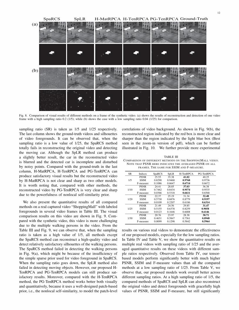
12

SpaRCS SpLR H-MatRPCA H-TenRPCA PG-TenRPCA

(a)

Ground-Truth

(b)

Fig. 8. Comparison of visual results of different methods on a frame of the synthetic video. (a) shows the results of reconstruction and detection of one videoframe with a high sampling ratio 0.2 (1/5); while (b) shows the case with a low sampling ratio 0.04 (1/25) for comparison.

sampling ratio (SR) is taken as 1/5 and 1/25 respectively.The last column shows the ground-truth videos and silhouettesof video foregrounds. It can be observed that, when thesampling ratio is a low value of 1/25, the SpaRCS methodtotally fails in reconstructing the original video and detectingthe moving car. Although the SpLR method can producea slightly better result, the car in the reconstructed videois blurred and the detected car is incomplete and disturbedby noisy points. Compared with the ground-truth in the lastcolumn, H-MatRPCA, H-TenRPCA and PG-TenRPCA canproduce satisfactory visual results but the reconstructed videoby H-MatRPCA is not clear and sharp as two other models.It is worth noting that, compared with other methods, thereconstructed video by PG-TenRPCA is very clear and sharpdue to the powerfulness of nonlocal self-similarity prior.

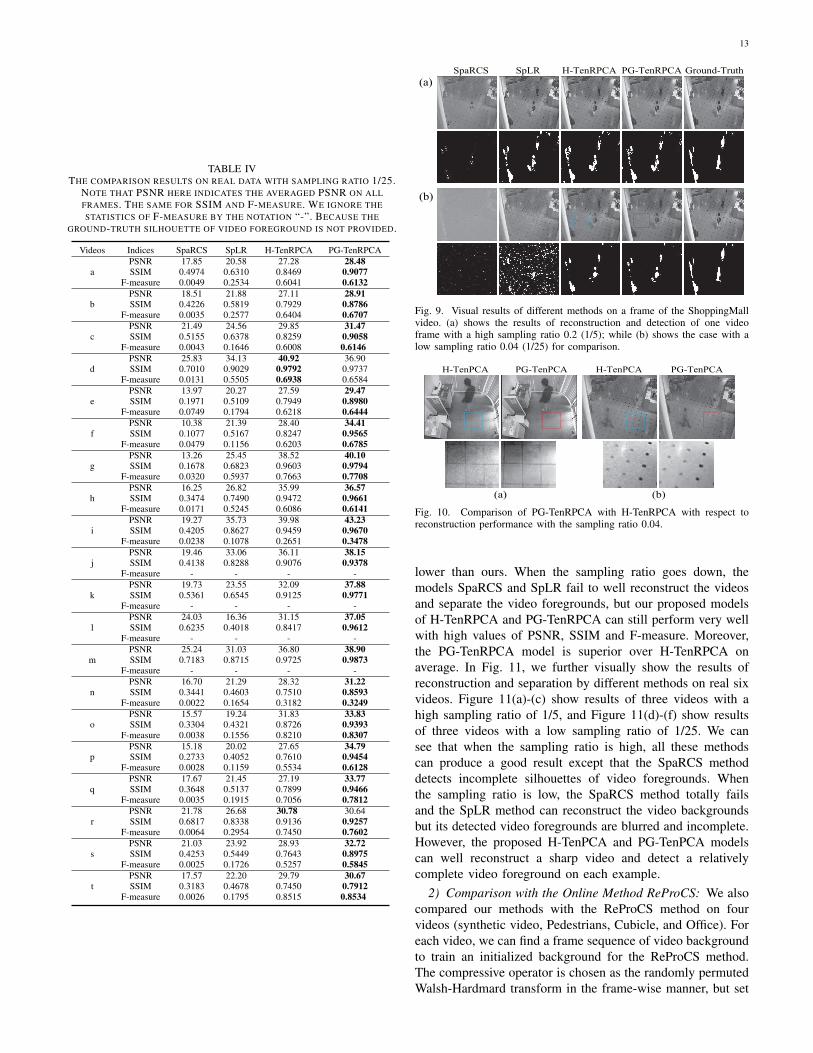
We also present the quantitative results of all comparedmethods on a real captured video “ShoppingMall” with labeledforegrounds in several video frames in Table III. The visualcomparison results on this video are shown in Fig. 9. Com-pared with the synthetic video, this video is more challengingdue to the multiple walking persons in the video. From theTable III and Fig. 9, we can observe that, when the samplingratio is taken as a high value of 1/5, all methods exceptthe SpaRCS method can reconstruct a high-quality video anddetect relatively satisfactory silhouettes of the walking persons.The SpaRCS method failed in detecting the walking personsin Fig. 9(a), which might be because of the insufficiency ofthe simple sparse prior used for video foreground in SpaRCS.When the sampling ratio goes down, the SpLR method alsofailed in detecting moving objects. However, our proposed H-TenRPCA and PG-TenRPCA models can still produce sat-isfactory results. Moreover, compared with the H-TenRPCAmethod, the PG-TenRPCA method works better both visuallyand quantitatively, because it uses a well-designed patch-basedprior, i.e., the nonlocal self-similarity, to model the patch-level

correlations of video background. As shown in Fig. 9(b), thereconstructed region indicated by the red box is more clear andsharper than the region indicated by the light blue box (Bestseen in the zoom-in version of pdf), which can be furtherillustrated in Fig. 10. We further provide more experimental

TABLE IIICOMPARISON OF DIFFERENT METHODS ON THE SHOPPINGMALL VIDEO.

NOTE THAT PSNR HERE INDICATES THE AVERAGED PSNR ON ALLFRAMES. THE SAME FOR SSIM AND F-MEASURE.

SR Indices SpaRCS SpLR H-TenRPCA PG-TenRPCA

1/5PSNR 25.55 35.38 41.02 40.25SSIM 0.8290 0.9468 0.9768 0.9736

F-measure 0.1086 0.6647 0.6714 0.6672

1/10PSNR 24.41 28.85 37.03 36.38SSIM 0.7462 0.8434 0.9574 0.9535

F-measure 0.0366 0.5318 0.6611 0.6568

1/20PSNR 22.37 25.19 31.34 32.48SSIM 0.5730 0.6876 0.8779 0.9197

F-measure 0.0109 0.2207 0.6186 0.6314

1/25PSNR 21.49 24.56 29.85 31.47SSIM 0.5155 0.6378 0.8259 0.9058

F-measure 0.0123 0.1646 0.6008 0.6146

1/30PSNR 20.76 23.97 28.38 30.71SSIM 0.4651 0.5847 0.7561 0.8948

F-measure 0.0099 0.1298 0.5842 0.5964

results on various real videos to demonstrate the effectivenessof our proposed models, especially for the low sampling ratios.In Table IV and Table V, we show the quantitative results onmultiple real videos with sampling ratio of 1/25 and the aver-aged quantitative results on these videos with different sam-ple ratios respectively. Observed from Table IV, our tensor-based models perform significantly better with much higherPSNR, SSIM and F-measure values than all the comparedmethods at a low sampling ratio of 1/25. From Table V, weobserve that, our proposed models work overall better acrossdifferent sampling ratios. At a high sampling ratio of 1/5, thecompared methods of SpaRCS and SpLR can also reconstructthe original video and detect foregrounds with gracefully highvalues of PSNR, SSIM and F-measure, but still significantly

13

TABLE IVTHE COMPARISON RESULTS ON REAL DATA WITH SAMPLING RATIO 1/25.

NOTE THAT PSNR HERE INDICATES THE AVERAGED PSNR ON ALLFRAMES. THE SAME FOR SSIM AND F-MEASURE. WE IGNORE THESTATISTICS OF F-MEASURE BY THE NOTATION “-”. BECAUSE THE

GROUND-TRUTH SILHOUETTE OF VIDEO FOREGROUND IS NOT PROVIDED.

Videos Indices SpaRCS SpLR H-TenRPCA PG-TenRPCA

aPSNR 17.85 20.58 27.28 28.48SSIM 0.4974 0.6310 0.8469 0.9077

F-measure 0.0049 0.2534 0.6041 0.6132

bPSNR 18.51 21.88 27.11 28.91SSIM 0.4226 0.5819 0.7929 0.8786

F-measure 0.0035 0.2577 0.6404 0.6707

cPSNR 21.49 24.56 29.85 31.47SSIM 0.5155 0.6378 0.8259 0.9058

F-measure 0.0043 0.1646 0.6008 0.6146

dPSNR 25.83 34.13 40.92 36.90SSIM 0.7010 0.9029 0.9792 0.9737

F-measure 0.0131 0.5505 0.6938 0.6584

ePSNR 13.97 20.27 27.59 29.47SSIM 0.1971 0.5109 0.7949 0.8980

F-measure 0.0749 0.1794 0.6218 0.6444

fPSNR 10.38 21.39 28.40 34.41SSIM 0.1077 0.5167 0.8247 0.9565

F-measure 0.0479 0.1156 0.6203 0.6785

gPSNR 13.26 25.45 38.52 40.10SSIM 0.1678 0.6823 0.9603 0.9794

F-measure 0.0320 0.5937 0.7663 0.7708

hPSNR 16.25 26.82 35.99 36.57SSIM 0.3474 0.7490 0.9472 0.9661

F-measure 0.0171 0.5245 0.6086 0.6141

iPSNR 19.27 35.73 39.98 43.23SSIM 0.4205 0.8627 0.9459 0.9670

F-measure 0.0238 0.1078 0.2651 0.3478

jPSNR 19.46 33.06 36.11 38.15SSIM 0.4138 0.8288 0.9076 0.9378

F-measure - - - -

kPSNR 19.73 23.55 32.09 37.88SSIM 0.5361 0.6545 0.9125 0.9771

F-measure - - - -

lPSNR 24.03 16.36 31.15 37.05SSIM 0.6235 0.4018 0.8417 0.9612

F-measure - - - -

mPSNR 25.24 31.03 36.80 38.90SSIM 0.7183 0.8715 0.9725 0.9873

F-measure - - - -

nPSNR 16.70 21.29 28.32 31.22SSIM 0.3441 0.4603 0.7510 0.8593

F-measure 0.0022 0.1654 0.3182 0.3249

oPSNR 15.57 19.24 31.83 33.83SSIM 0.3304 0.4321 0.8726 0.9393

F-measure 0.0038 0.1556 0.8210 0.8307

pPSNR 15.18 20.02 27.65 34.79SSIM 0.2733 0.4052 0.7610 0.9454

F-measure 0.0028 0.1159 0.5534 0.6128

qPSNR 17.67 21.45 27.19 33.77SSIM 0.3648 0.5137 0.7899 0.9466

F-measure 0.0035 0.1915 0.7056 0.7812

rPSNR 21.78 26.68 30.78 30.64SSIM 0.6817 0.8338 0.9136 0.9257

F-measure 0.0064 0.2954 0.7450 0.7602

sPSNR 21.03 23.92 28.93 32.72SSIM 0.4253 0.5449 0.7643 0.8975

F-measure 0.0025 0.1726 0.5257 0.5845

tPSNR 17.57 22.20 29.79 30.67SSIM 0.3183 0.4678 0.7450 0.7912

F-measure 0.0026 0.1795 0.8515 0.8534

SpaRCS SpLR H-TenRPCA PG-TenRPCA Ground-Truth

(a)

(b)

Fig. 9. Visual results of different methods on a frame of the ShoppingMallvideo. (a) shows the results of reconstruction and detection of one videoframe with a high sampling ratio 0.2 (1/5); while (b) shows the case with alow sampling ratio 0.04 (1/25) for comparison.

(a) (b)

H-TenPCA PG-TenPCA H-TenPCA PG-TenPCA

Fig. 10. Comparison of PG-TenRPCA with H-TenRPCA with respect toreconstruction performance with the sampling ratio 0.04.

lower than ours. When the sampling ratio goes down, themodels SpaRCS and SpLR fail to well reconstruct the videosand separate the video foregrounds, but our proposed modelsof H-TenRPCA and PG-TenRPCA can still perform very wellwith high values of PSNR, SSIM and F-measure. Moreover,the PG-TenRPCA model is superior over H-TenRPCA onaverage. In Fig. 11, we further visually show the results ofreconstruction and separation by different methods on real sixvideos. Figure 11(a)-(c) show results of three videos with ahigh sampling ratio of 1/5, and Figure 11(d)-(f) show resultsof three videos with a low sampling ratio of 1/25. We cansee that when the sampling ratio is high, all these methodscan produce a good result except that the SpaRCS methoddetects incomplete silhouettes of video foregrounds. Whenthe sampling ratio is low, the SpaRCS method totally failsand the SpLR method can reconstruct the video backgroundsbut its detected video foregrounds are blurred and incomplete.However, the proposed H-TenPCA and PG-TenPCA modelscan well reconstruct a sharp video and detect a relativelycomplete video foreground on each example.

2) Comparison with the Online Method ReProCS: We alsocompared our methods with the ReProCS method on fourvideos (synthetic video, Pedestrians, Cubicle, and Office). Foreach video, we can find a frame sequence of video backgroundto train an initialized background for the ReProCS method.The compressive operator is chosen as the randomly permutedWalsh-Hardmard transform in the frame-wise manner, but set

14

TABLE VTHE AVERAGED RESULTS OF DIFFERENT METHODS ON VARIOUS REAL

VIDEOS.

SR Indices SpaRCS SpLR H-TenRPCA PG-TenRPCA

1/5PSNR 27.50 38.26 42.42 41.13SSIM 0.7812 0.9488 0.9788 0.9756

F-measure 0.1946 0.6269 0.6799 0.6803

1/10PSNR 23.48 32.34 39.41 38.13SSIM 0.6206 0.8430 0.9629 0.9599

F-measure 0.0424 0.5368 0.6756 0.6760

1/20PSNR 19.53 26.84 35.01 35.51SSIM 0.4665 0.7049 0.9153 0.9396

F-measure 0.0158 0.3105 0.6393 0.6536

1/25PSNR 18.54 24.48 31.82 34.46SSIM 0.4203 0.6245 0.8575 0.9301

F-measure 0.0155 0.2514 0.6213 0.6475

1/30PSNR 17.87 24.36 31.15 33.86SSIM 0.3943 0.6026 0.8239 0.9245

F-measure 0.0150 0.2369 0.6202 0.6389

(b)

Ground-Truth SpaRCS SpLR H-TenRPCA PG-TenRPCA

(c)

(d)

(e)

(f)

(a)

Fig. 11. The reconstruction and separation (RS) results of different methodson six videos. The first three videos show the RS results for a high samplingratio 0.2, while the last three videos for a low sampling ratio 0.04.

TABLE VICOMPARISON WITH THE ONLINE METHOD REPROCS. “SYN” INDICATESTHE SYNTHETIC VIDEO. VIDEOS (F), (H), AND (P) ARE SHOWN IN FIG. 6.

Video Indices ReProCS H-TenRPCA PG-TenRPCASampling Ratio = 0.75

synPSNR 25.56 22.34 41.6157SSIM 0.9612 0.5858 0.9890

F-measure 0.8767 0.8664 0.8652

(f)PSNR 15.23 17.62 42.29SSIM 0.8160 0.4119 0.9891

F-measure 0.8098 0.8218 0.8120

(h)PSNR 16.93 23.84 42.71SSIM 0.8780 0.5312 0.9832

F-measure 0.7136 0.8217 0.7324

(p)PSNR 14.45 16.48 45.09SSIM 0.6838 0.3295 0.9905

F-measure 0.6845 0.8524 0.8383Sampling Ratio = 0.5

synPSNR 25.32 19.12 33.7437SSIM 0.9509 0.4322 0.9541

F-measure 0.8730 0.8569 0.8540

(f)PSNR 15.13 14.16 36.44SSIM 0.7948 0.2739 0.9668

F-measure 0.8021 0.8184 0.8141

(h)PSNR 16.95 20.48 36.02SSIM 0.8760 0.3931 0.9375

F-measure 0.7129 0.8057 0.7437

(p)PSNR 14.52 13.12 38.98SSIM 0.6146 0.2225 0.9688

F-measure 0.6876 0.8395 0.8289Sampling Ratio = 0.25

synPSNR 24.94 17.22 24.42SSIM 0.9360 0.3281 0.7054

F-measure 0.8617 0.8548 0.8434

(f)PSNR 14.99 12.31 21.37SSIM 0.7524 0.1874 0.6263

F-measure 0.7537 0.7820 0.7890

(h)PSNR 17.02 18.59 26.68SSIM 0.8756 0.3225 0.7092

F-measure 0.7090 0.8110 0.8073

(p)PSNR 13.69 11.16 20.67SSIM 0.4529 0.1548 0.5502

F-measure 0.5284 0.8368 0.8151

as the same for each frame because of the constraint ofthe ReProCS method on compressive operator, i.e., Ad =D ·H ·P (d = 1, 2, · · · , D). The sampling ratios in this groupof experiments are set as 0.75, 0.5, and 0.25, respectively.

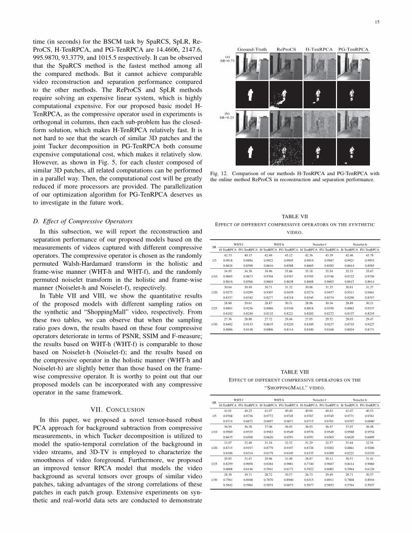
We exhibit the reconstruction and separation results inTable VI. From this table, we can find that our proposedmethods almost outperform the ReProCS method in terms ofF-measure index for video separation (foreground detection).This good detection performance on video foreground can beattributed to the favor of spatio-temporal continuity from 3Dtotal variation. Moreover, for video reconstruction, the PG-TenRPCA method is superior over methods H-TenRPCA andReProCS in terms of PSNR and SSIM indices. Additionally,when the sampling ratio is very low, on some videos, e.g.,the synthetic video and video (p), the ReProCS method canreconstruct a better video than the H-TenPRCA method interms of SSIM and PSNR indices. This is because the pre-trained video background provides sufficient information forthe ReProCS method; however, for our proposed methods,the pre-training procedure is not required. These findingscan be further supported in Fig. 12, where we exhibit thereconstruction and separation results of one video with a highsampling ratio of 0.75 and a low sampling ratio of 0.25.

3) Computational Speeds: We compare the running time ofdifferent models on the resized video “ShoppingMall” of thesize 64 × 64 × 128. It is noted that this kind of comparisonin terms of the running time is only illustrative. The running

15

time (in seconds) for the BSCM task by SpaRCS, SpLR, Re-ProCS, H-TenRPCA, and PG-TenRPCA are 14.4606, 2147.6,995.9870, 93.3779, and 1015.5 respectively. It can be observedthat the SpaRCS method is the fastest method among allthe compared methods. But it cannot achieve comparablevideo reconstruction and separation performance comparedto the other methods. The ReProCS and SpLR methodsrequire solving an expensive linear system, which is highlycomputational expensive. For our proposed basic model H-TenRPCA, as the compressive operator used in experiments isorthogonal in columns, then each sub-problem has the closed-form solution, which makes H-TenRPCA relatively fast. It isnot hard to see that the search of similar 3D patches and thejoint Tucker decomposition in PG-TenRPCA both consumeexpensive computational cost, which makes it relatively slow.However, as shown in Fig. 5, for each cluster composed ofsimilar 3D patches, all related computations can be performedin a parallel way. Then, the computational cost will be greatlyreduced if more processors are provided. The parallelizationof our optimization algorithm for PG-TenRPCA deserves usto investigate in the future work.

D. Effect of Compressive Operators

In this subsection, we will report the reconstruction andseparation performance of our proposed models based on themeasurements of videos captured with different compressiveoperators. The compressive operator is chosen as the randomlypermuted Walsh-Hardamard transform in the holistic andframe-wise manner (WHT-h and WHT-f), and the randomlypermuted noiselet transform in the holistic and frame-wisemanner (Noiselet-h and Noiselet-f), respectively.

In Table VII and VIII, we show the quantitative resultsof the proposed models with different sampling ratios onthe synthetic and “ShoppingMall” video, respectively. Fromthese two tables, we can observe that when the samplingratio goes down, the results based on these four compressiveoperators deteriorate in terms of PSNR, SSIM and F-measure;the results based on WHT-h (WHT-f) is comparable to thosebased on Noiselet-h (Noiselet-f); and the results based onthe compressive operator in the holistic manner (WHT-h andNoiselet-h) are slightly better than those based on the frame-wise compressive operator. It is worthy to point out that ourproposed models can be incorporated with any compressiveoperator in the same framework.

VII. CONCLUSION

In this paper, we proposed a novel tensor-based robustPCA approach for background subtraction from compressivemeasurements, in which Tucker decomposition is utilized tomodel the spatio-temporal correlation of the background invideo streams, and 3D-TV is employed to characterize thesmoothness of video foreground. Furthermore, we proposedan improved tensor RPCA model that models the videobackground as several tensors over groups of similar videopatches, taking advantages of the strong correlations of thesepatches in each patch group. Extensive experiments on syn-thetic and real-world data sets are conducted to demonstrate

(a)SR=0.75

(b)SR=0.25

Ground-Truth ReProCS H-TenRPCA PG-TenRPCA

Fig. 12. Comparison of our methods H-TenRPCA and PG-TenRPCA withthe online method ReProCS in reconstruction and separation performance.

TABLE VIIEFFECT OF DIFFERENT COMPRESSIVE OPERATORS ON THE SYNTHETIC

VIDEO.

SRWHT-f WHT-h Noiselet-f Noiselet-h

H-TenRPCA PG-TenRPCA H-TenRPCA PG-TenRPCA H-TenRPCA PG-TenRPCA H-TenRPCA PG-TenRPCA

1/5

42.33 40.15 42.48 43.12 42.36 43.39 42.46 43.78

0.9918 0.9894 0.9922 0.9945 0.9919 0.9947 0.9921 0.9953

0.8624 0.8598 0.8616 0.8588 0.8605 0.8582 0.8614 0.8585

1/10

34.95 34.38 34.96 35.86 35.18 35.54 35.33 35.67

0.9695 0.9673 0.9704 0.9767 0.9705 0.9746 0.9722 0.9756

0.8616 0.8566 0.8604 0.8638 0.8608 0.8603 0.8615 0.8614

1/20

30.64 30.40 30.71 31.32 30.88 31.35 30.81 31.37

0.9275 0.9299 0.9307 0.9459 0.9274 0.9457 0.9311 0.9461

0.8337 0.8342 0.8277 0.8318 0.8345 0.8374 0.8290 0.8357

1/25

28.80 29.61 28.87 30.31 28.96 30.34 28.89 30.21

0.8901 0.9236 0.8966 0.9349 0.8818 0.9350 0.8962 0.9337

0.8182 0.8240 0.8132 0.8221 0.8202 0.8272 0.8137 0.8219

1/30

27.36 28.88 27.72 29.46 27.05 29.52 28.03 29.47

0.8492 0.9133 0.8635 0.9229 0.8189 0.9237 0.8710 0.9227

0.8086 0.8148 0.8006 0.8114 0.8100 0.8168 0.8024 0.8171

TABLE VIIIEFFECT OF DIFFERENT COMPRESSIVE OPERATORS ON THE

“SHOPPINGMALL” VIDEO.

SRWHT-f WHT-h Noiselet-f Noiselet-h

H-TenRPCA PG-TenRPCA H-TenRPCA PG-TenRPCA H-TenRPCA PG-TenRPCA H-TenRPCA PG-TenRPCA

1/5

41.01 40.25 41.07 40.40 40.94 40.43 41.07 40.53

0.9768 0.9736 0.9772 0.9745 0.9767 0.9745 0.9771 0.9761

0.6714 0.6672 0.6697 0.6671 0.6715 0.6701 0.6707 0.6680

1/10

36.94 36.38 37.06 36.45 36.93 36.47 37.07 36.48

0.9569 0.9535 0.9583 0.9549 0.9576 0.9549 0.9588 0.9554

0.6635 0.6568 0.6626 0.6591 0.6591 0.6565 0.6620 0.6609

1/20

31.07 32.48 31.34 32.52 31.29 32.57 31.64 32.54

0.8715 0.9197 0.8779 0.9197 0.8726 0.9202 0.8861 0.9206

0.6186 0.6314 0.6179 0.6345 0.6155 0.6309 0.6221 0.6310

1/25

29.85 31.47 29.96 31.49 28.87 30.11 30.57 31.41

0.8259 0.9058 0.8384 0.9081 0.7740 0.9047 0.8414 0.9060

0.6008 0.6146 0.5941 0.6172 0.5922 0.6082 0.5964 0.6126

1/30

28.38 30.71 28.72 30.57 26.73 29.49 28.71 30.57

0.7561 0.8948 0.7870 0.8940 0.6315 0.8911 0.7868 0.8916

0.5842 0.5964 0.5874 0.6073 0.5677 0.5852 0.5764 0.5937

16

the superiority of proposed approaches over the existing state-of-the-art approaches.

In the future work, we are interested in the followingresearch directions. First, model the layers of the foregroundsusing mixture of Gaussian to enhance its encoding capabilityfor complex configured foreground. Second, develop bettermodel for the complex background, such as dynamic back-ground with illumination change, smog or snow, and so on.Third, incorporate the motion of cameras into our proposedmodels. Finally, develop online version of our approach tomake it more effective, thus facilitating the further use formore practical scenarios.

APPENDIX A

This optimization problem can be approximately solvedby the alternating direction method (ADM). Firstly, fixingthe orthogonal factors U1p, U2p, U3, and U4p, we have||Rp(X1)−Gp×1U1p×2U2p×3U3×4U4p||2F = ||Rp(X1)×1

UT1p ×2 U

T2p ×3 U

T3 ×4 U

T4p − Gp||2F . Hence, it follows that

Gp = Rp(X1)×1 UT1p ×2 U

T2p ×3 U

T3 ×4 U

T4p.

Then, using the solution of Gp we further derive that

‖Rp(X1)− Gp ×1 U1p ×2 U2p ×3 U3 ×4 U4p‖2F =

‖Rp(X1)‖2F − 2〈Rp(X1),Gp ×1 U1p ×2 U2p ×3 U3 ×4 U4p〉+ ||Gp||2F =

||Rp(X1)||2F − ||Rp(X1)×1 UT1p ×2 U

T2p ×3 U

T3 ×4 U

T4p||2F .

The factor matrix U1p can be estimated by maximizing||Rp(X1) ×1 UT

1p ×2 UT2p ×3 UT

3 ×4 UT4p||2F with respect

to U1p. It then easily follows that U1p = SVD(Rp(X1) ×2

UT2p ×3 U

T3 ×4 U

T4p)(1), r1

). Here, SVD(A, r) indicates top

r singular vectors of matrix A. Likewise, we can obtain thesolutions for factor matrixes U2p and U4p. Finally, the factormatrix U3 can be estimated by maximizing

∑p ||Rp(X1)×1

UT1p ×2 UT

2p ×3 U3 ×4 UT4p||2F with respect to U3. It is

easy to find that U3 = eigs(∑P

p=1 ZpZTp , r3

), where Zp =(

Rp(X1)×1UT1p×2U

T2p×4U

T4p

)(3)

and eigs(A, r) indicatestop r eigen vectors of matrix A.

ACKNOWLEDGMENT

The authors would like to thank the associate editor andthe anonymous reviewers for their insightful comments, whichled to a significant improvement of this paper. The authorsalso would like to thank Dr. Waters, Dr. Deng, as well as Dr.Guo for sharing the codes of the SpaRCS method, the SpLRmethod, and the ReProCS method, respectively.

REFERENCES

[1] M. Piccardi, “Background subtraction technieques: a review,” in Proc.IEEE Int. Conf. on Systems, Man and Cybernetics, vol. 4, pp. 3099–3104,2004.

[2] T. Bouwmans, “Recent advanced statistical background modelling forforeground detection: A systematic survey,” Recent Patents Comput. Sci.,vol. 4, no. 3, pp. 147–176, 2011.

[3] S. Brutzer, B. Hoferlin and G. Heidemann, “Evaluation of backgroundsubtraction techniques for video surveillance,” In Proc. IEEE Comput.Soc. Conf. Comput. Vis. Pattern Recognit., June 2011, 1937-1944.

[4] Y. Benezeth, P. M. Jodoin, B. Emile, H. Laurent and C. Rosenberger,“Comparative study of background subtraction algorithms,” J. Eelectron.Imaging, vol. 19, no. 3, pp. 033003, 2010.

[5] A. Sobral and A. Vacavant, “A comprehensive review of backgroundsubtraction algorithms evaluated with synthetic and real videos,” Comput.Vis. Image Understand., vol. 122, pp. 4–21, May 2014.

[6] T. Bouwmans, “Traditional and recent approaches in background model-ing for foreground detection: An overview,” Computer Science Review,vol. 11–12, pp. 31–66, May 2014.

[7] T. Wang, A.G. Backhouse, and I. Y. H. Gu, “Online subspace learningon Grassmann manifold for moving object tracking in video”, in Proc.IEEE Int. Conf. Acoust., Speech, Signal Process., 2008, pp. 969–972.

[8] C. Beleznai, B. Fruhstuck, and H. Bischof, “Multiple object trackingusing local PCA”, in Proc. 18th International Conference on PatternRecognition, 2006, pp. 79–82.

[9] M. Lamarre and J.J. Clark, “Background subtraction using competingmodels in the block-DCT domain”, in Proc. 16th International Confer-ence on Pattern Recognition, 2002, pp. 299–302.

[10] A. Aggarwal, S. Biswas, S. Singh, S. Sural, and A. K. Majumdar,“Object tracking using background subtraction and motion estimation inMPEG videos”, in Proc. 7th Asian Conference on Computer Vision, 2006,pp. 121–130.

[11] E. Candes, J. Romberg, and Tao, T. “Robust uncertainty principles: exactvector reconstruction from highly incomplete frequency information”.IEEE Trans. Inf. Theory vol. 52, no. 2, pp. 489-509, 2006.

[12] D. Donoho, “Compressed sensing”, IEEE Trans. Inf. Theory, vol. 52,no. 4, pp. 1280–1306, 2006.

[13] E. Candes and T. Tao, “Near-optimal signal recovery from randomprojections: universal encoding strategies”, IEEE Trans. Inf. Theory, vol.52, no. 12, pp. 5406–5425, 2006.

[14] D. Takhar, J. N. Laska, M. Wakin, M. F. Duarte, D. Baron, S. Sarvotham,K. Kelly, and R.G. Baraniuk, “A new compressive imaging camera Ar-chitecture using optical-domain compression” in Proc. of ComputationalImaging IV at SPIE Electronic Imaging, Jan. 2006, pp. 43–52.

[15] M. Wakin, J. N. Laska, M. F. Duarte, D. Baron, S. Sarvotham, D. Takhar,K. Kelly, and R.G. Baraniuk, “An architecture for compressive imaging”,in Proc.IEEE Int. Conf. Image Process., Oct. 2006, pp. 1273–1276,.

[16] M. Wakin, J. N. Laska, M. F. Duarte, D. Baron, S. Sarvotham, D. Takhar,K. Kelly, and R. G. Baraniuk, “Compressive imaging for video represen-tation and coding”, in Proc. of Picture Coding Symposium, Beijing, China,April 2006.

[17] M. F. Duarte, M. A. Davenport, D. Takhar, J. N. Laska, T. Sun, K.F. Kelly, and R. G. Baraniuk, “Single pixel imaging via compressivesampling,” IEEE Signal Process. Mag., vol. 25, no. 2, pp. 83–91, 2008.

[18] V. Cevher, A. Sankaranarayanan, M. Duarte, D. Reddy, R. Baraniuk,and R. Chellappa, “Compressive sensing for background subtraction,” InProc. Eur. Conf. Comput. Vis, 2008, pp. 155–168.

[19] A. E. Waters, A. C. Sankaranarayanan, and R. G. Baraniuk, “SpaRCS:Recovering low-rank and sparse matrices from compressive measure-ments,” In Proc. Adv. Neural Inf. Process. Syst., 2011, pp.1089–1097.

[20] H. Guo, C. L. Qiu, and N. Vaswani, “An online algorithm for separatingsparse and low-dimensional signal sequences from their sum,” IEEETrans. on Signal Process., vol. 62, no. 16, pp. 4284–4297, 2014.

[21] H. Jiang, W. Deng, and Z. Shen, “Surveillance video processing usingcompressive sensing,” Inverse Probl. Imag., vol. 6, no. 2, pp. 201–214,2012.

[22] H. Jiang, S. Zhao, Z. Shen, W. Deng, P. Wilford, and R. Haimi-Cohen,“Surveillance video analysis using compressive sensing with low latency,”Bell Labs Technical Journal, vol. 18, no. 4, pp. 63–74, 2014.

[23] N. M. Oliver, B. Rosario, and A. P. Pentland, “A Bayesian computervision system for modeling human interactions,” IEEE Trans. PatternAnal. Mach. Intell., vol. 22, pp. 831–843, 2000.

[24] E. J. Candes, X. Li, Y. Ma, and J. Wright, “Robust principal componentanalysis?” J. ACM, vol. 58, no. 3, pp. 1–39, 2011.

[25] X. Zhou, C. Yang and W. Yu, “Moving object detection by detectingcontiguous outliers in the low-rank represention,” IEEE Trans. PatternAnal. Mach. Intell.., vol. 35, no. 3, pp. 59–610, 2013.

[26] Z. Gao, L. F. Cheong, and Y. X. Wang, “Block-sparse RPCA for salientmotion detection,” IEEE Trans. Pattern Anal. Mach. Intell., vol. 36, no.10, pp. 1975–1987, 2014.

[27] X. C. Cao, L. Yang and X. J. Guo, “Total variation regularized RPCAfor irregularly moving object detection under dynamic background”, IEEETrans. on Cybernetics, accepted, 2015.

[28] X. J. Guo, X. G. Wang, Y. Liang, X. C. Cao and Y. Ma, “Robustforeground detection using smoothness and arbitrariness constraints,” InProc. Eur. Conf. Comput. Vis, 2014, pp. 535–550.

17

[29] X. Ding, L. He, and L. Carin, “Bayesian robust principal componentanalysis,” IEEE Trans. on Image Process., vol. 20, no. 12, pp. 3419–3430, 2011.

[30] S. D. Babacan, M. Luessi, R. Molina, and A. K. Katsaggelos, “SparseBayesian methods for low-rank matrix estimation,” IEEE Trans. on SignalProcess., vol. 60, no. 8, pp. 3964–3977, 2012.

[31] Q. Zhao, D. Y. Meng, Z. B. Xu, W. M. Zuo, and L. Zhang, “Robustprincipal component analysis with complex noise,” In Proc. Int. Conf.Mach. Learn., 2014, pp. 55–63.

[32] J. Rymel, J. Renno, D. Greenhill, J. Orwell, and G. A. Jones, “Adpativeeigen-backgrounds for object detection,” in Proc. IEEE Int. Conf. ImageProcess., 2004, pp. 1847–1850.

[33] R. Li, Y. Chen, and X. Zhang, “Fast robust eigen-background updatingfor foreground detection,” in Proc. IEEE Int. Conf. Image Process., 2006,pp.1833–1836.

[34] L. Balzano, R. Nowak, and B. Recht, “Online identification and trackingof subspaces from highly incomplete information”, in Proc. 48th AnnualAllerton Conference On Communication, Control, and Computing (Aller-ton), September 2010, pp. 704–711.

[35] J. He, L. Balzano, and J. Lui, “Online robust subspace tracking frompartial information”, [Online]. Available: http://arxiv.org/abs/1109.3827.

[36] J. He, L. Balzano, and A. Szlam, “Incremental gradient on the Grass-mannian for online foreground and background separation in subsampledvideo,” in Proc. IEEE Comput. Soc. Conf. Comput. Vis. Pattern Recognit.,2012, pp. 1568–1575.

[37] L. Balzano and S. J. Wright, “Local convergence of an algorithm forsubspace identification from partial data”, Found. Comput. Math., pp. 1-36, October 2014.

[38] J. Xu, V. Ithapu, L. Mukherjee, J. Rehg, and V. Singh, “GOSUS:Grassmannian online subspace updates with strutured-sparsity,” in Proc.IEEE Int. Conf. Comput. Vis., 2013, pp. 3376–3383.

[39] Y. Chi, Y. C. Eldar, and R. Calderbank. “Petrels: Parallel subspace esti-mation and tracking by recursive least squares from partial observations”,IEEE Trans. on Signal Process., vol. 61, no. 23, pp. 5947–5959, 2013.

[40] J. F. C. Mota, N. Deligiannis, and M. Rodrigues, “Compressed sens-ing with prior information: Optimal strategies, geometry, and bounds”,[Online]. Available: http://arxiv.org/abs/1408.5250.

[41] J. F. C. Mota, N. Deligiannis, A. C. Sankaranarayanan, V. Cevher,and M. Rodrigues, “Adaptive-rate sparse signal reconstruction with ap-plication in compressive background subtraction”, [Online]. Available:http://arxiv.org/abs/1503.03231.

[42] N. D. Sidiropoulos and A. Kyrillidis, “Multi-way compressed sensing forsparse low-rank tensors”, IEEE Signal Proc. Let., vol. 9, no.11, pp.757-760, 2012.

[43] S. Friedland, Q. Li and D Schonfeld, “Compressive sensing of sparsetensors”, [Online]. Available:http://arxiv.org/abs/1305.5777.

[44] R. Coifman, F. Geshwind, and Y. Meyer, “Noiselets”, Appl. Comp.Harmonic Analysis, vol. 10, pp. 27-44, 2001.

[45] T. G. Kolda and B. W. Bader, “Tensor decompositions and applications,”SIAM review, vol. 51, no. 3, pp. 455–500, 2009.

[46] A. Cichocki, R. Zdunek and A. H. Phan et al, “Nonnegative matrix andtensor factorizations: applications to exploratory multi-way data analysisand blind source separation,” John Wiley & Sons, 2009.

[47] T. T. Do, L. Gan, N. H. Nguyen, et al, “Fast and efficient compressivesensing using structurally random matrices,” IEEE Trans. on SignalProcess., vol. 60, no. 1, pp. 139–154, 2012.

[48] J. Mairal, F. Bach, J. Ponce, G. Sapiro, and A. Zisserman, “Non-localsparse models for image restoration,” In Proc. IEEE 12th Int. Conf.Comput., 2009.

[49] W. Dong, G. Shi, and X. Li, “Nonlocal image restoration with bilat-eral variance estimation: a low-rank approach,” IEEE Trans. on ImageProcess., vol. 22, no. 2, pp. 700–711, 2013.

[50] W. Dong, G. Shi, X. Li, Y. Ma, and F. Huang, “Compressive sensingvia nonlocal low-rank regularization,” IEEE Trans. on Image Process.,vol. 23, no. 8, pp. 3618–3632, 2014.

[51] J. Sun and M. F. Tappen, “Learning non-local range Markov randomfield for image restoration,” In Proc. IEEE Comput. Soc. Conf. Comput.Vis. Pattern Recognit., 2011, pp. 2272–2279.

[52] Y. Peng, D. Y. Meng, Z. B. Xu, C. Q. Gao, Y. Yang, and B. Zhang,“Decomposable nonlocal tensor dictionary learning for multispectralimage denoising,” In Proc. IEEE Comput. Soc. Conf. Comput. Vis. PatternRecognit., 2014, pp. 4321–4328.

[53] S. Boyd, N. Parikh, E. Chu, B. Peleato, and J. Eckstein, “Distributedoptimization and statistical learning via the alternating direction methodof multipliers,” Foundations and Trends in Machine Learning, vol. 3, pp.1–122, 2011.

[54] W. Deng, M. J. Lai, Z. Peng, et al., “Parallel multi-block ADMM withO(1/k) convergence,” [Online]. Available: http://arxiv.org/abs/1312.3040.

[55] J. F. C. Mota, J. M. F. Xavier, P. M. Q. Aguiar, and M. Poschel, “D-ADMM: A communication-efficient distributed algorithm for separableoptimization,” IEEE Trans. on Signal Process., vol. 61, no. 10, pp. 2718–2723, 2013.

[56] Y. Shen, Z. Wen, and Y. Zhang, “Augmented Lagrangian alternatingdirection method for matrix separation based on low-rank factorization,”Optimization Methods Software, vol. 29, no. 2, pp. 239–263, Mar. 2014.

[57] M. Y. Hong, Z. Q. Luo, “On the linear convergence of thealternating direction method of multipliers,” [Online]. Available:http://arxiv.org/abs/1208.3922.

[58] P. Robinson, E. H. Tappenden, “A flexible ADMM algorithm for bigdata applications,” [Online]. Available: http://arxiv.org/abs/1502.04391.

[59] Z. Wang, A. C. Bovik, H. R. Sheikh, and E. P. Simoncelli, “Imagequality assessment: From error visibility to structural similarity,” IEEETrans. on Image Process., vol. 13, no. 4, pp. 600–612, 2004.

[60] The EC Funded CAVIAR project/IST 2001 37540, [Online]. Available:http://homepages.inf.ed.ac.uk/rbf/CAVIAR/.

[61] L. Li, W. Huang, I. Gu, and Q. Tian, “Statistical modeling of complexbackgrounds for foreground object detection,” IEEE Trans. on ImageProcess., vol. 13, no. 11, pp. 1459–1472, 2004.

[62] V. Mahadevan and N. Vasconcelos, “Spatiotemporal saliency in highlydynamic scences,” IEEE Trans. Pattern Anal. Mach. Intell., vol. 32, no.1, pp. 171–177, 2010.

[63] N. Goyette, P. M. Jodoin, F. Porikli, J. Konrad, and P. lshwar,“Changedaetection.net: a new change detection benchmark dataset,” InProc. IEEE Comput. Soc. Conf. Comput. Vis. Pattern Recognit., 2012,pp. 1–8.

Wenfei Cao received the Ph.D. degree in computerscience from Xi’an Jiaotong University, China, in2015. He worked as a visiting student in RIKENBSI, Japan, from Nov. 2012 to Oct. 2013. He iscurrently an assistant professor at the Departmentof Applied Mathematics in ShaanXi Normal Uni-versity. His current research interests include sparseoptimization, randomized numerical linear algebra,and computer vision.

Yao Wang received the Ph.D. degree in appliedmathematics from Xi’an Jiaotong University, China,in 2014. He worked as a visiting student in GeorgiaInstitute of Technology form Oct. 2010 to Nov.2011. He is currently an assistant professor at theDepartment of Statistics in Xi’an Jiaotong Univer-sity. His current research interests include statisticalsignal processing, high-dimensional statistical infer-ence, large-scale video analysis, and computationalbiology.

Jian Sun received the Ph.D. degree in appliedmathematics from Xi’an Jiaotong University, China,in 2009. He worked as a visiting student in MicrosoftResearch Asia from Nov. 2005 to Mar. 2008, apost-doctoral researcher in University of CentralFlorida from Aug. 2009 to Apr. 2010, and a post-doctoral researcher in willow project team of EcoleNormale Superieure de Paris and INRIA from Sept.2012 to Aug. 2014. He is currently an associateprofessor with the Institute for Information and Sys-tem Sciences, Xi’an Jiaotong University. His current

research interests include computer vision and image processing.

18

Deyu Meng received the Ph.D. degree in computerscience from Xi’an Jiaotong University, China, in2008. He is currently an associate professor with theInstitute for Information and System Sciences, Xi’anJiaotong University. From 2012 to 2014, he took histwo-year sabbatical leave in Carnegie Mellon Uni-versity. His current research interests include self-paced learning, noise modeling, weekly supervisedlearning, and tensor sparsity.

Can Yang received the Ph.D. degree in electronicand computer engineering from the Hong KongUniversity of Science and Technology in 2011. Heworked as an associate researcher scientist at YaleUniversity, New Haven, Connecticut. He is currentlyan assistant professor at the Department of Mathe-matics, Hong Kong Baptist University. His researchinterests include Biostatistics, machine learning, andpattern recognition.

Andrzej Cichocki received the Ph.D. and Dr.Sc.(Habilitation) degrees, all in electrical engineering,from Warsaw University of Technology, Poland. Heis currently the senior team leader of the Laboratoryfor Advanced Brain Signal Processing at RIKENBSI, Japan. He is coauthor of more than 400 sci-entific papers and 4 monographs. He served as AEof IEEE Transactions on Signal Processing, NeuralNetworks and Learning Systems, Cybernetics. He isa fellow of the IEEE.

Zongben Xu received his Ph.D. degree in mathemat-ics from Xi’an Jiaotong University, China, in 1987.He now serves as the Chief Scientist of NationalBasic Research Program of China (973 Project),and Director of the Institute for Information andSystem Sciences of Xi’an Jiaotong University. Hewas elected as member of Chinese Academy ofScience in 2011. His current research interests in-clude intelligent information processing and appliedmathematics.