Carson River: Total Maximum Daily Loads for Total Suspended Solids and Turbidity FINAL Approved by EPA: September 25, 2007

Bureau of Water Quality Planning Nevada Division of Environmental Protection Department of Conservation and Natural Resources

2

Table of Contents Executive Summary ...................................................................................................................................... 4 1.0 Introduction ........................................................................................................................................ 5 1.1 Total Maximum Daily Load defined.............................................................................................. 5 1.1.1 Problem Statement .......................................................................................................... 5 1.1.2 Source Analysis ............................................................................................................... 5 1.1.3 Target Analysis ................................................................................................................ 5 1.1.4 Pollutant Load Capacity and Allocation ........................................................................... 6 1.1.5 Approach to TMDL Adoption and Implementation........................................................... 6 1.2 Watershed Plan ........................................................................................................................... 6 2.0 Background ....................................................................................................................................... 6 2.1 Study Area ................................................................................................................................... 7 2.2 Major Monitoring Stations and TMDL Sites ................................................................................. 7 2.3 Water Quantity ............................................................................................................................. 9 2.4 Existing Water Quality Standards and Aquatic Beneficial Uses ................................................ 10 2.5 303(d) Listing ............................................................................................................................. 12 2.6 Relationship between Water Quality and Historic Hydrologic and Geomorphic Alteration ....... 13 3.0 Total Suspended Solids/Turbidity TMDL....................................................................................... 15 3.1 Problem Statement .................................................................................................................... 15 3.2 Relationship between TSS and Turbidity................................................................................... 18 3.3 Source Analysis ......................................................................................................................... 21 3.4 Target Analysis .......................................................................................................................... 27 3.5 Pollutant Load Capacity and Allocation ..................................................................................... 27 3.6 Estimated Load Allocations and Reductions ............................................................................. 29 3.7 Next Steps/Future Needs........................................................................................................... 31 3.7.1 Supplemental Monitoring ............................................................................................... 31 3.7.2 Assessment of Physical Condition................................................................................. 32 3.7.3 Water Quality Standard Updates ................................................................................... 32 3.8 Schedule of TMDL Updates or Revisions.................................................................................. 33 References ................................................................................................................................................. 34 Appendices Appendix A Monthly Mean Flows for Selected Gaging Stations............................................................ 37 Appendix B Flow Duration Curves for Selected Gaging Stations.......................................................... 39 Appendix C Seasonal Box Plots: TSS ................................................................................................... 41 Appendix D Seasonal Box Plots: Turbidity ............................................................................................ 43 Appendix E Load Duration Curves: TSS................................................................................................ 45 Appendix F Load Duration Curves: TSS as Surrogate for Turbidity...................................................... 48 Appendix G Load Reduction Estimates for TSS .................................................................................... 50 Appendix H Load Reduction Estimates for TSS as Surrogate for Turbidity .......................................... 52 List of Tables Table 1 TMDL Sites .................................................................................................................................. 7 Table 2 Water Quality Standards for Total Phosphorus, Total Suspended Solids, Turbidity ................. 11 Table 3 Selected Results from Newcombe and MacDonald (1991)....................................................... 12 Table 4 Comparison of the 1998 and 2002 303(d) Lists ........................................................................ 13 Table 5 Summary of TSS Data .............................................................................................................. 17 Table 6 Summary of Turbidity Data ........................................................................................................ 17 Table 7 % Exceedance of the TSS and Turbidity Standards ................................................................ 17

3

List of Tables continued Table 8 TSS vs. Turbidity Regression Equations for the 5 TMDL Sites ................................................. 19 Table 9 TSS Surrogates Corresponding to the Turbidity Standards ..................................................... 20 Table 10 Kendall’s Tau Correlation Analysis for the Period of Record ................................................... 25 Table 11 Kendall’s Tau Correlation Analysis by Season ........................................................................ 25 Table 12 Duration Curve Exceedances for the Period of Record ........................................................... 28 Table 13 Duration Curve Exceedances by Season ................................................................................ 28 Table 14 Estimated Load Reductions for Mexican Gage ....................................................................... 30 Table 15 % April-June Sample Loads Equal to or Exceeding Curve: TSS ............................................ 31 Table 16 % April-June Sample Loads Equal to or Exceeding Curve: TSS as surrogate for Turbidity ..... 31 List of Figures Figure 1 Carson River Basin Water Quality Monitoring Stations and TMDL Sites .................................... 8 Figure 2 Mean Monthly Streamflow for the East Fork Carson River near Gardnerville ............................ 9 Figure 3 Flow Duration Curve for the East Fork Carson River near Gardnerville ................................... 10 Figure 4 Schematic of Reaches Impaired for TSS and Turbidity............................................................. 16 Figure 5 % Exceedances of Beneficial Use Standards ........................................................................... 18 Figure 6 Relationship between TSS and Turbidity ................................................................................. 20 Figure 7 Distribution of TSS Concentrations .......................................................................................... 23 Figure 8 Distribution of Turbidity Values ................................................................................................ 23 Figure 9 Seasonal Distribution of Turbidity Values................................................................................. 24 Figure 10 Seasonal Distribution of TSS Concentrations .......................................................................... 24 Figure 11 Seasonal Median Concentrations............................................................................................. 26 Figure 12 Seasonal Median Loads .......................................................................................................... 26 Figure 13 Load Duration Curve Carson River at Mexican Gage: TSS as Surrogate ............................... 29 Figure 14 Estimated Observed and Allowable Loads for Mexican Gage: TSS as Surrogate ................. 30

4

Carson River Total Maximum Daily Loads – Total Suspended Solids and Turbidity

Executive Summary Section 303(d) of the Clean Water Act requires each state to develop a list of water bodies that need additional work beyond existing controls to achieve or maintain water quality standards, and submit an updated list to the Environmental Protection Agency (EPA) every two years. The Section 303(d) List provides a comprehensive inventory of water bodies impaired by all sources. CFR (Code of Federal Regulations) 40 Part 130.7 requires states to develop TMDLs (Total Maximum Daily Loads) for the waterbody/pollutant combinations appearing in the 303(d) List. The Nevada 2004 303(d) Lists identify Total Phosphorus, Total Suspended Solids, Turbidity, Temperature, Total Iron, Total Mercury and Dissolved Zinc as parameters of concern for the Carson River. Fecal Coliform and E. coli have also been identified as parameters of concern on the West Fork from Stateline to Muller Lane in Carson Valley. This document will present TMDLs for Total Suspended Solids and Turbidity. All of these 303(d) Listings were based upon ambient water quality monitoring conducted at 15 different sampling points established by the Nevada Division of Environmental Protection. The data indicates that single value concentrations for Total Suspended Solids are exceeded at only two sites. The Turbidity single value standard is exceeded at four of the monitoring sites. Analysis also indicates that, in general, TSS and Turbidity concentrations increase in the downstream direction to Mexican Gage but decrease downstream to Weeks Bridge. This TMDL report includes a discussion of the following categories:

• Problem Statement • Source Analysis • Target Analysis • Pollutant Load Capacity and Allocation • Future Needs

Through the use of equations and load duration curves, the defined TMDLs and load allocations vary with flow thereby addressing the EPA requirement to consider seasonal variations and critical flow conditions in the TMDL process. This document presents an adaptive management approach to the Carson River TMDLs. This approach is used in situations where data needed to determine the TMDL and associated load allocations are limited, but enables the adoption and implementation of a TMDL while collecting additional information (“Guidance for Water Quality Based Decisions—The TMDL Process” (#EPA 440/4-91-001, April 1991)). The adaptive management approach enables states to use available information to establish preliminary targets, begin to implement needed controls and restoration actions, monitor waterbody response to these actions, and plan for future TMDL review and revision. As this approach, a number of future needs have been identified for further refinement of the Total Suspended Solids and Turbidity TMDLs:

• Evaluate water quality data collected by the Conservation Districts and the Desert Research

Institute • Assess physical condition and relate characteristics such as the percentage of riparian vegetation

or percentage of incised banks within a reach to the degree of water quality impairment or lack of biological integrity

• Determine if updates to the Total Suspended Solids or Turbidity standards are warranted As time and resources allow, the Nevada Division of Environmental Protection will address these needs and update the TMDLs as appropriate.

5

Carson River Total Maximum Daily Loads – Total Suspended Solids and Turbidity

1.0 Introduction

The primary goal of the Clean Water Act (CWA) is to restore and maintain the chemical, physical and biological integrity of the Nation’s waters. CWA Section 303(a) requires each state to adopt water quality standards that include beneficial uses of the waters and criteria to protect the uses. The U.S. Environmental Protection Agency (USEPA) must approve these standards. Section 303(d) of the CWA requires each state to develop a list of water bodies that need additional work beyond existing controls to achieve or maintain water quality standards, and submit an updated list to the EPA every two years. The Section 303(d) List provides a comprehensive inventory of water bodies impaired by all sources. The Nevada 2004 303(d) List (approved in November 2005) identifies Total Phosphorus (TP), Total Suspended Solids (TSS), Turbidity, Temperature, Total Iron, Total Mercury and Dissolved Zinc as parameters of concern for the Carson River. Section 303(d) also requires states to develop Total Maximum Daily Loads (TMDLs) for the waterbody/pollutant combinations appearing in the 303(d) list. The TMDL process provides an organized framework to develop watershed-based solutions for 303(d) listed waters. This document will present TMDLs for Total Suspended Solids and Turbidity only. TMDLs for TP were developed separately and approved by EPA in November 2005. No schedule has been set for temperature, iron, mercury or zinc. It should be noted that this TMDL is not applicable on Tribal property. As a sovereign nation, the Washoe Tribe of Nevada and California is responsible for developing water quality standards and TMDLs within the boundaries of their land. 1.1 Total Maximum Daily Load (TMDL) Defined TMDLs are an assessment of the amount of pollutant a water body can receive and not violate water quality standards. Also, TMDLs provide a means to integrate the management of both point and nonpoint sources of pollution through the establishment of waste load allocations for point source discharges and load allocations for nonpoint sources. For pollutants other than heat, TMDLs are to be established at levels necessary to attain and maintain the applicable narrative and numerical water quality standards with consideration given to seasonal variations and a margin of safety. To achieve the necessary pollutant reductions, wasteload allocations for point source discharges are implemented through National Pollutant Discharge Elimination System (NPDES) permits for point source discharges. Nonpoint source (NPS) TMDLs can be implemented through voluntary or regulatory nonpoint source control programs, depending on the state. In Nevada, participation in programs to control nonpoint source pollution is voluntary, which lends a degree of uncertainty as to whether pollutant reductions attributed to load allocations can be achieved. As development in the Carson River Basin continues, however, nonpoint source pollution generated by urban sources and discharged through stormwater runoff will be managed through the NPDES Stormwater Program. While each TMDL report is unique, many contain similar elements. Following is a discussion of the typical components that may appear in a TMDL based upon USEPA guidance (October 1999). 1.1.1 Problem Statement: Describes the key factors and background information that characterize the nature of the impairment, such as chemical water quality, biological integrity, physical condition, etc. 1.1.2 Source Analysis: Identifies known loading sources (both point and nonpoint sources) by location, type, frequency, and magnitude to the extent possible. Characterizing nonpoint sources can be difficult and often requires significant financial resources. 1.1.3 Target Analysis: Identifies those future conditions needed for compliance with the water quality standards and for support of the beneficial use. The target analyses clarifies whether the ultimate goal of

6

the TMDL is to comply with a numeric water quality criterion, comply with an interpretation of a narrative water quality criterion, or attain a desired condition that supports meeting a specified designated use. 1.1.4 Pollutant Load Capacity and Allocation: Identifies the waterbody loading capacity. The loading capacity is the maximum amount of pollutant loading a waterbody can assimilate without violating the TMDL target. The allowable loadings are then distributed or “allocated” among the significant sources of the pollutant. A margin of safety is included in the analysis to account for uncertainty in the relationship between pollutant loads and the water quality of the receiving water. It can also be stated that the margin of safety is to account for uncertainties in meeting the water quality standards when the target and TMDL are met. Additionally, consideration needs to be given to seasonal variations and critical conditions. The general equation describing the TMDL with the allocation and margin of safety components is given below:

TMDL = Sum of WLA + Sum LA + Margin of Safety (Eq. 1) Where:

Sum of WLA = sum of wasteload allocations given to point sources Sum of LA = sum of load allocations given to nonpoint sources According to the CFR 130.2(i), TMDLs need not be expressed in pounds per day when alternative means are better suited for the waterbody problem. In recent years some states have utilized (and USEPA has approved) a load duration curve analysis to establish target load reductions. 1.1.5 Load Duration Curves and an Adaptive Management Approach to TMDL Adoption and Implementation The State of Nevada is pursuing an adaptive management approach to TMDL development and implementation for the Carson River using Duration Curve Analysis. A preliminary target for load reduction can be established, while continuing to collect information that will help determine the relationship between a water quality (WQ) standard and an aquatic beneficial use, such as cold-water fish. Using a Load Duration Curve as a “TMDL” provides the flexibility to conduct long-term physical, biological and chemical monitoring to establish a credible link between the appropriate water quality standard, the load reduction target and the Beneficial Use. By establishing this relationship, the “TMDL” will be a more meaningful tool in tracking improvements in water quality or overall health of the system as controls and restoration activities are implemented. The TMDL process is an adaptive management approach designed to help meet the primary goal of the Clean Water Act – to restore and maintain the chemical, physical and biological integrity of the Nation’s waters. 1.2 Watershed Plan Although not specifically required by the CWA, a plan to implement the TMDLs is often developed. Point source waste load allocations are managed through NPDES permits. In most states, including Nevada, the nonpoint source load allocations are addressed through voluntary compliance with assistance from the CWA Section 319 grant program. In 2002, the USEPA began focusing the use of a portion of 319 NPS funds to the development of NPS TMDLs, development of TMDL or watershed-based implementation plans, and implementation of the plans. The watershed plans are intended to focus activities on measures that will reduce non point source pollutant loads and restore impaired waters. Watershed-based plans developed with 319 funds must include nine elements: (1) pollution sources; (2) an estimate of load reductions needed; (3) description of NPS management measures needed; (4) technical, financial or regulatory needs to implement plan; (5) public education; (6) an implementation schedule for NPS management measures; (7) measurable milestones; (8) criteria for determining if load reductions are being met and WQ standards attained; and (9) a monitoring component. NDEP is currently working with the Carson Water Subconservancy District to develop a Watershed Plan for the Carson River that contains the nine key elements. 2.0 Background

7

2.1 Study Area Although the headwaters of the Carson River originate in Alpine County, California, approximately 85% or 3360 square miles of the Carson River Watershed lies in Nevada (Nevada Division of Water Planning, 1997). The source of the East Fork is near Sonora Pass and the West Fork begins as several small streams that merge below Carson Pass near the Red Lake area along Highway 88 (California Department of Water Resources, 1991). The two forks combine in Carson Valley and the main stem travels northeast through Carson City, Dayton Valley and are eventually impounded by Lahontan Reservoir. Flows from the reservoir are controlled for downstream irrigation in the Fallon area and the river terminates in the Carson Sink. Water is also diverted into the Stillwater Wildlife Management Area. The predominant land use in the basin valleys is agriculture. However, the Minden-Gardnerville, Carson City and Dayton areas are experiencing extensive development. Ranch property is being sold and subdivided, forever changing the rural character of the Carson River Watershed. Increased population growth may have a significant impact on future water quality and the focus of nonpoint source pollution control programs. 2.2 Major Monitoring Stations and TMDL Sites There are 15 sampling locations on the Carson River that are routinely monitored by NDEP (Figure 1). Bryant Creek water quality and the impacts of Leviathan Mine were addressed under a separate TMDL document, which was approved by EPA in November 2003. The Truckee Canal and Below Lahontan stations will be evaluated as part of a possible future TMDL for Lahontan Reservoir. All water quality data evaluated for this report can be provided electronically upon request. Duration Curve Analysis was conducted at five of the remaining 12 sampling locations because of the proximity of the USGS Flow Gages to the monitoring sites. Table 1 outlines the “TMDL” sites, the corresponding reaches and USGS gaging stations. If the Load Duration Curve is exceeded at the selected site according to the target established for non-attainment, then the entire upstream reach will not meet the TMDL. TABLE 1 “TMDL” Sites, Corresponding Reaches and USGS Gaging Stations for the Carson River

“TMDL” Site Impaired for TSS or Turbidity?

Corresponding Reach upstream of TMDL Site and the Nevada Administrative Code (NAC) segments within TMDL Reaches

USGS Gaging Station

1 West Fork at Paynesville, Ca. No Duration Curves developed to illustrate change in water quality at downstream sites

Woodfords # 10310000

2 East Fork at Riverview - at Washoe Bridge, downstream of power dam & upstream of mobile home park

Turbidity only East Fork at Riverview to the Stateline 445A.150 TSS Duration Curve developed to illustrate change in water quality at downstream sites

Near Gardnerville # 10309000

3 Carson River at Mexican Gage TSS & Turbidity

Mexican Gage to the West Fork at Muller & on the East Fork to Muller for TSS 445A.152, 445A.153, 445A.154 Mexican Gage to the Stateline on the West Fork and to the East Fork at Riverview for Turbidity 445A.151, 445A.152, 445A.153, 445A.154

Near Carson City # 10311000

4 Carson River at New Empire Bridge Turbidity only

From New Empire to Mexican Gage 445A.155 TSS Duration Curve developed for to illustrate change in water quality at downstream site

Deer Run Road # 10311400

5 Carson River at Weeks Bridge TSS & Turbidity Weeks to New Empire for TSS 445A.156, 445A.157 Weeks to Dayton for Turbidity 445A.157

Near Fort Churchill # 10312000

8

9

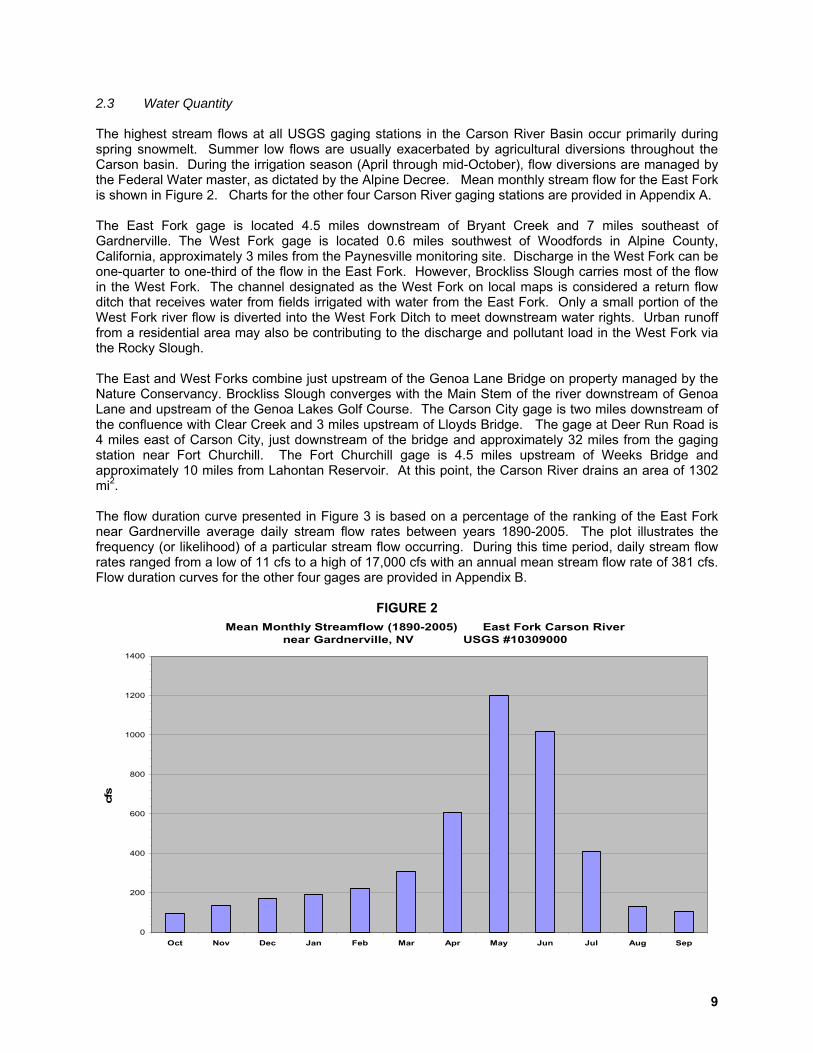
2.3 Water Quantity The highest stream flows at all USGS gaging stations in the Carson River Basin occur primarily during spring snowmelt. Summer low flows are usually exacerbated by agricultural diversions throughout the Carson basin. During the irrigation season (April through mid-October), flow diversions are managed by the Federal Water master, as dictated by the Alpine Decree. Mean monthly stream flow for the East Fork is shown in Figure 2. Charts for the other four Carson River gaging stations are provided in Appendix A. The East Fork gage is located 4.5 miles downstream of Bryant Creek and 7 miles southeast of Gardnerville. The West Fork gage is located 0.6 miles southwest of Woodfords in Alpine County, California, approximately 3 miles from the Paynesville monitoring site. Discharge in the West Fork can be one-quarter to one-third of the flow in the East Fork. However, Brockliss Slough carries most of the flow in the West Fork. The channel designated as the West Fork on local maps is considered a return flow ditch that receives water from fields irrigated with water from the East Fork. Only a small portion of the West Fork river flow is diverted into the West Fork Ditch to meet downstream water rights. Urban runoff from a residential area may also be contributing to the discharge and pollutant load in the West Fork via the Rocky Slough. The East and West Forks combine just upstream of the Genoa Lane Bridge on property managed by the Nature Conservancy. Brockliss Slough converges with the Main Stem of the river downstream of Genoa Lane and upstream of the Genoa Lakes Golf Course. The Carson City gage is two miles downstream of the confluence with Clear Creek and 3 miles upstream of Lloyds Bridge. The gage at Deer Run Road is 4 miles east of Carson City, just downstream of the bridge and approximately 32 miles from the gaging station near Fort Churchill. The Fort Churchill gage is 4.5 miles upstream of Weeks Bridge and approximately 10 miles from Lahontan Reservoir. At this point, the Carson River drains an area of 1302 mi2. The flow duration curve presented in Figure 3 is based on a percentage of the ranking of the East Fork near Gardnerville average daily stream flow rates between years 1890-2005. The plot illustrates the frequency (or likelihood) of a particular stream flow occurring. During this time period, daily stream flow rates ranged from a low of 11 cfs to a high of 17,000 cfs with an annual mean stream flow rate of 381 cfs. Flow duration curves for the other four gages are provided in Appendix B.

FIGURE 2 Mean Monthly Streamflow (1890-2005) East Fork Carson River

near Gardnerville, NV USGS #10309000

0

200

400

600

800

1000

1200

1400

Oct Nov Dec Jan Feb Mar Apr May Jun Jul Aug Sep

cfs

10

FIGURE 3

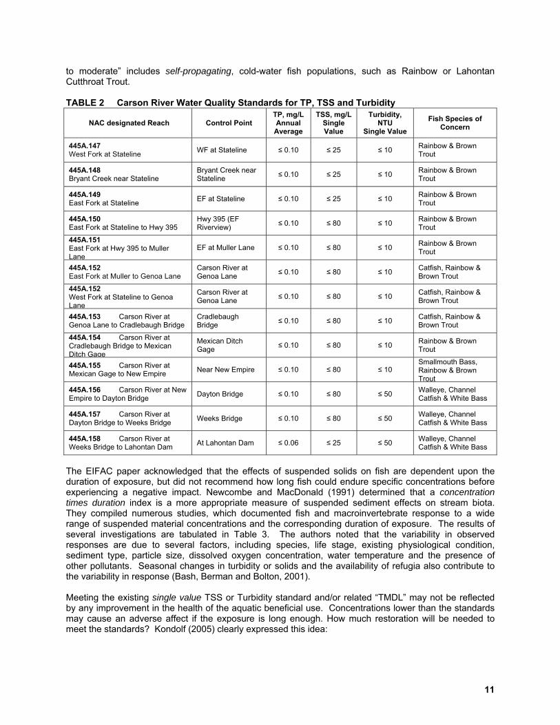
2.4 Existing Water Quality Standards & Aquatic Beneficial Uses The 2004 Nevada 303(d) List identifies TP, TSS, Turbidity, Temperature, Total Iron, Total Mercury and Dissolved Zinc as parameters of concern. This report will only present TMDLs for TSS and Turbidity. The TP TMDL was approved in November 2005. If deemed appropriate, the other parameters may be addressed at a later date in separate documents. The existing water quality standards for TP, TSS and Turbidity are listed in Table 2 and are derived from the Nevada Administrative Code (NAC) Section 445A.147 through 445A.158. The control points listed in the NAC identify the downstream monitoring station of each reach. If a standard is exceeded at a control point, the entire reach is considered impaired. The beneficial uses for the Carson River are listed in NAC 445A.146 and includes propagation of aquatic life, irrigation, watering of livestock, recreation involving contact with water, recreation not involving contact with water, industrial supply, municipal or domestic supply or both, and the propagation of wildlife. The Upper Carson River Watershed, which extends from the California Stateline to the New Empire Bridge at Deer Run Road in Carson City, is described as a cold-water fishery. Species of major concern are also identified in Table 2. From New Empire down to Lahontan Dam, the system is considered a warm water fishery. Section 303 (c)(2)(A) of the Clean Water Act requires states to consider the beneficial uses when revising or adopting a new water quality standard. However, the standards may not truly represent healthy conditions for the specified beneficial use in the water body. It appears that the turbidity standards established for the Carson River were taken from the water quality criteria published by the Federal Water Pollution Control Administration in 1968 (The “Green” Book), which recommended 10 JTU for cold water streams and 50 JTU for warm water streams. According to the “Blue Book” (National Academy of Sciences and Engineering, 1972), 80 mg/L TSS represents “moderate protection” for fisheries. This criterion was adopted into the Nevada Administrative Code in 1984 as a Single Value Standard. EPA derived this value from a 1965 report issued by the European Inland Fisheries Advisory Commission (EIFAC), which reported that “good to moderate” fisheries could be maintained in waters containing 25 - 80 mg/L TSS. A concentration of 25 mg/L would provide a high level of protection. It is unclear if “good

11

to moderate” includes self-propagating, cold-water fish populations, such as Rainbow or Lahontan Cutthroat Trout. TABLE 2 Carson River Water Quality Standards for TP, TSS and Turbidity

NAC designated Reach Control Point TP, mg/L Annual

Average

TSS, mg/L Single Value

Turbidity, NTU

Single Value Fish Species of

Concern

445A.147 West Fork at Stateline WF at Stateline ≤ 0.10 ≤ 25 ≤ 10 Rainbow & Brown

Trout

445A.148 Bryant Creek near Stateline

Bryant Creek near Stateline ≤ 0.10 ≤ 25 ≤ 10 Rainbow & Brown

Trout

445A.149 East Fork at Stateline EF at Stateline ≤ 0.10 ≤ 25 ≤ 10 Rainbow & Brown

Trout

445A.150 East Fork at Stateline to Hwy 395

Hwy 395 (EF Riverview) ≤ 0.10 ≤ 80 ≤ 10 Rainbow & Brown

Trout

445A.151 East Fork at Hwy 395 to Muller Lane

EF at Muller Lane ≤ 0.10 ≤ 80 ≤ 10 Rainbow & Brown Trout

445A.152 East Fork at Muller to Genoa Lane

Carson River at Genoa Lane ≤ 0.10 ≤ 80 ≤ 10 Catfish, Rainbow &

Brown Trout

445A.152 West Fork at Stateline to Genoa Lane

Carson River at Genoa Lane ≤ 0.10 ≤ 80 ≤ 10 Catfish, Rainbow &

Brown Trout

445A.153 Carson River at Genoa Lane to Cradlebaugh Bridge

Cradlebaugh Bridge ≤ 0.10 ≤ 80 ≤ 10 Catfish, Rainbow &

Brown Trout

445A.154 Carson River at Cradlebaugh Bridge to Mexican Ditch Gage

Mexican Ditch Gage ≤ 0.10 ≤ 80 ≤ 10 Rainbow & Brown

Trout

445A.155 Carson River at Mexican Gage to New Empire Near New Empire ≤ 0.10 ≤ 80 ≤ 10

Smallmouth Bass, Rainbow & Brown Trout

445A.156 Carson River at New Empire to Dayton Bridge Dayton Bridge ≤ 0.10 ≤ 80 ≤ 50 Walleye, Channel

Catfish & White Bass

445A.157 Carson River at Dayton Bridge to Weeks Bridge Weeks Bridge ≤ 0.10 ≤ 80 ≤ 50 Walleye, Channel

Catfish & White Bass

445A.158 Carson River at Weeks Bridge to Lahontan Dam At Lahontan Dam ≤ 0.06 ≤ 25 ≤ 50 Walleye, Channel

Catfish & White Bass

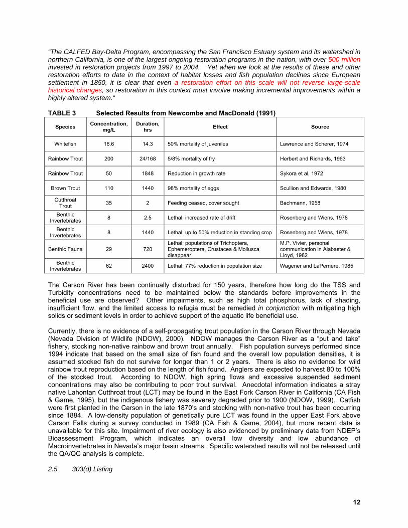
The EIFAC paper acknowledged that the effects of suspended solids on fish are dependent upon the duration of exposure, but did not recommend how long fish could endure specific concentrations before experiencing a negative impact. Newcombe and MacDonald (1991) determined that a concentration times duration index is a more appropriate measure of suspended sediment effects on stream biota. They compiled numerous studies, which documented fish and macroinvertebrate response to a wide range of suspended material concentrations and the corresponding duration of exposure. The results of several investigations are tabulated in Table 3. The authors noted that the variability in observed responses are due to several factors, including species, life stage, existing physiological condition, sediment type, particle size, dissolved oxygen concentration, water temperature and the presence of other pollutants. Seasonal changes in turbidity or solids and the availability of refugia also contribute to the variability in response (Bash, Berman and Bolton, 2001). Meeting the existing single value TSS or Turbidity standard and/or related “TMDL” may not be reflected by any improvement in the health of the aquatic beneficial use. Concentrations lower than the standards may cause an adverse affect if the exposure is long enough. How much restoration will be needed to meet the standards? Kondolf (2005) clearly expressed this idea:

12

“The CALFED Bay-Delta Program, encompassing the San Francisco Estuary system and its watershed in northern California, is one of the largest ongoing restoration programs in the nation, with over 500 million invested in restoration projects from 1997 to 2004. Yet when we look at the results of these and other restoration efforts to date in the context of habitat losses and fish population declines since European settlement in 1850, it is clear that even a restoration effort on this scale will not reverse large-scale historical changes, so restoration in this context must involve making incremental improvements within a highly altered system.“ TABLE 3 Selected Results from Newcombe and MacDonald (1991)

Species Concentration, mg/L

Duration, hrs Effect Source

Whitefish 16.6 14.3 50% mortality of juveniles Lawrence and Scherer, 1974

Rainbow Trout 200 24/168 5/8% mortality of fry Herbert and Richards, 1963

Rainbow Trout 50 1848 Reduction in growth rate Sykora et al, 1972

Brown Trout 110 1440 98% mortality of eggs Scullion and Edwards, 1980

Cutthroat Trout 35 2 Feeding ceased, cover sought Bachmann, 1958

Benthic Invertebrates 8 2.5 Lethal: increased rate of drift Rosenberg and Wiens, 1978

Benthic Invertebrates 8 1440 Lethal: up to 50% reduction in standing crop Rosenberg and Wiens, 1978

Benthic Fauna 29 720 Lethal: populations of Trichoptera, Ephemeroptera, Crustacea & Mollusca disappear

M.P. Vivier, personal communication in Alabaster & Lloyd, 1982

Benthic Invertebrates 62 2400 Lethal: 77% reduction in population size Wagener and LaPerriere, 1985

The Carson River has been continually disturbed for 150 years, therefore how long do the TSS and Turbidity concentrations need to be maintained below the standards before improvements in the beneficial use are observed? Other impairments, such as high total phosphorus, lack of shading, insufficient flow, and the limited access to refugia must be remedied in conjunction with mitigating high solids or sediment levels in order to achieve support of the aquatic life beneficial use. Currently, there is no evidence of a self-propagating trout population in the Carson River through Nevada (Nevada Division of Wildlife (NDOW), 2000). NDOW manages the Carson River as a “put and take” fishery, stocking non-native rainbow and brown trout annually. Fish population surveys performed since 1994 indicate that based on the small size of fish found and the overall low population densities, it is assumed stocked fish do not survive for longer than 1 or 2 years. There is also no evidence for wild rainbow trout reproduction based on the length of fish found. Anglers are expected to harvest 80 to 100% of the stocked trout. According to NDOW, high spring flows and excessive suspended sediment concentrations may also be contributing to poor trout survival. Anecdotal information indicates a stray native Lahontan Cutthroat trout (LCT) may be found in the East Fork Carson River in California (CA Fish & Game, 1995), but the indigenous fishery was severely degraded prior to 1900 (NDOW, 1999). Catfish were first planted in the Carson in the late 1870’s and stocking with non-native trout has been occurring since 1884. A low-density population of genetically pure LCT was found in the upper East Fork above Carson Falls during a survey conducted in 1989 (CA Fish & Game, 2004), but more recent data is unavailable for this site. Impairment of river ecology is also evidenced by preliminary data from NDEP’s Bioassessment Program, which indicates an overall low diversity and low abundance of Macroinvertebretes in Nevada’s major basin streams. Specific watershed results will not be released until the QA/QC analysis is complete. 2.5 303(d) Listing

13

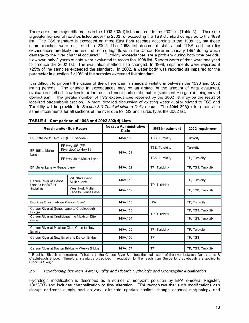
There are some major differences in the 1998 303(d) list compared to the 2002 list (Table 3). There are a greater number of reaches listed under the 2002 list exceeding the TSS standard compared to the 1998 list. The TSS standard is exceeded on three East Fork reaches according to the 1998 list, but these same reaches were not listed in 2002. The 1998 list document states that “TSS and turbidity exceedances are likely the result of record high flows in the Carson River in January 1997 during which damage to the river channel occurred.” Turbidity exceedances are a problem during both time periods. However, only 2 years of data were evaluated to create the 1998 list; 5 years worth of data were analyzed to produce the 2002 list. The evaluation method also changed. In 1998, impairments were reported if >25% of the samples exceeded the standard. In 2002, a water body was reported as impaired for the parameter in question if >10% of the samples exceeded the standard. It is difficult to pinpoint the cause of the differences in standard violations between the 1998 and 2002 listing periods. The change in exceedances may be an artifact of the amount of data evaluated, evaluation method, flow levels or the result of more particulate matter (sediment + organic) being moved downstream. The greater number of TSS exceedances reported by the 2002 list may be the result of localized streambank erosion. A more detailed discussion of existing water quality related to TSS and Turbidity will be provided in Section 3.0 Total Maximum Daily Loads. The 2004 303(d) list reports the same impairments for all sections of the river due to TSS and Turbidity as the 2002 list. TABLE 4 Comparison of 1998 and 2002 303(d) Lists

Reach and/or Sub-Reach Nevada Administrative Code 1998 Impairment 2002 Impairment

EF Stateline to Hwy 395 (EF Riverview) 445A.150 TSS, Turbidity Turbidity

EF Hwy 395 (EF Riverview) to Hwy 88 TSS, Turbidity Turbidity

EF 395 to Muller Lane

EF Hwy 88 to Muller Lane

445A.151

TSS, Turbidity TP, Turbidity

EF Muller Lane to Genoa Lane 445A.152 TP, Turbidity TP, TSS, Turbidity

WF Stateline to Muller Lane 445A.152 TP, Turbidity Carson River at Genoa

Lane to the WF at Stateline West Fork Muller

Lane to Genoa Lane 445A.152 TP, Turbidity

TP, TSS, Turbidity

Brockliss Slough above Carson River* 445A.153 N/A TP, Turbidity

Carson River at Genoa Lane to Cradlebaugh Bridge 445A.153 TP, TSS, Turbidity

Carson River at Cradlebaugh to Mexican Ditch Gage 445A.154

TP, Turbidity TP, TSS, Turbidity

Carson River at Mexican Ditch Gage to New Empire 445A.155 TP, Turbidity TP, Turbidity

Carson River at New Empire to Dayton Bridge 445A.156 TP TP, TSS

Carson River at Dayton Bridge to Weeks Bridge 445A.157 TP TP, TSS, Turbidity

* Brockliss Slough is considered Tributary to the Carson River & enters the main stem of the river between Genoa Lane & Cradlebaugh Bridge. Therefore, standards proscribed in regulation for the reach from Genoa to Cradlebaugh are applied to Brockliss Slough. 2.6 Relationship between Water Quality and Historic Hydrologic and Geomorphic Modification Hydrologic modification is described as a source of nonpoint pollution by EPA (Federal Register, 10/23/03) and includes channelization or flow alteration. EPA recognizes that such modifications can disrupt sediment supply and delivery, eliminate riparian habitat, change channel morphology and

14

accelerate the delivery of pollutants to downstream areas. Projects that straighten, enlarge or relocate a stream channel may also require regular maintenance that will continually disturb the system (http://www.epa.gov/owow/nps/hydro.html). In 1996, a consulting firm (Inter-Fluve, Inc) conducted a fluvial geomorphic assessment of the Carson River in cooperation with a number of organizations and agencies within the watershed. The general conclusion drawn by the consultants is that the stability of the Carson River is poor and in a “state of geomorphic transition, and that further changes in channel geometry and planform can be expected”. They acknowledged that channel instability likely dates back to the initial use of the river by European settlers for irrigation and mining-related activities. In addition, efforts to control the large magnitude floods that occur periodically have resulted in levee construction and channelization. In 1965, the Bureau of Reclamation straightened approximately 70 out of the 114 miles of river between Stateline and Lahontan Reservoir. Channelization is cited as one of the principal reasons the Carson River is incised. Grazing and numerous dams and diversions are additional factors cited by Inter-Fluve that have contributed to system degradation. Livestock trample streambanks and may browse heavily on riparian vegetation, limiting natural regeneration. Permanent dam structures accumulate sediment that is flushed out during high flows, adding to the pollutant load. Push-up dams are constructed from riverbed materials and are often washed downstream during spring runoff. During low flow conditions, several reaches are subject to substantial dewatering because of water diverted for agricultural use. Based upon the existing observed physical condition, the water quality impairments in the Carson River may not simply be due to a direct discharge of some specified contaminant. Multiple disturbances to the river system, which began over a century ago, have altered form (meander pattern) and function, upsetting the balance between flow and sediment transport, disconnecting the river from its floodplain, lowering the water table and reducing pollutant assimilative capacity. Timber logged from the Upper East Fork Basin was transported down the Carson River to Empire City (top of Dayton Valley) to support Comstock mine construction. Floating logs down the Carson occurred over a 40-year time period, beginning in 1862 (NDWP, 1997). The largest drive was reported to be 4 miles long with logs stacked 8 feet high. Log drives would have had a tremendous impact on channel stability, by scouring the channel and destroying bank vegetation. Hydrogeomorphic alteration and habitat loss are considered the primary reasons the cold-water fishery is impaired. The impacts of logging, mining and irrigation led to increased bed and bank erosion, and the subsequent decline in water quality, macroinvertebrate populations and fish propagation. In many reaches, the Carson River has down-cut; creating shallow, over-widened channels with vertical banks that lack appropriate vegetation. The river channel also lacks adequate pool and riffle structure necessary for trout reproduction and survival in many reaches. NDOW (2000) reports that downstream of the town of Minden, sand and silt dominate the river bottom substrate. Initial evaluation of the pebble count data collected as part of NDEP’s Bioassessment Program supports NDOW’s claim. The median percentage of substrate determined to be < 2 mm is 67 percent at sites located just above the confluence at Genoa Lane and just above Cradlebaugh Bridge compared to 32 percent at the upstream sites on the East and West Forks. Sand or silt embedded in gravel used as spawning habitat can prevent trout from digging nests (redds) and may suffocate eggs already deposited (EIFAC, 1965). Changes to channel size and shape have occurred over the past 150 years. It is difficult to separate out the direct impacts from each occurrence because the physical changes have not been monitored. Over time, an incised stream will readjust at a lower base level, recreating a floodplain and establishing a new equilibrium. However, this new steady-state condition may be of less ecological value than what existed before the disturbance (Federal Interagency Stream Restoration Working Group, 1998). Continuous perturbations, such as mismanaged grazing in the riparian area or routine sand bar removal for conveyance will likely impede any readjustment, at least at the local reach level if not watershed-wide. Unchecked urban development in the floodplain, without buffer zones or conservation easements in place to preserve the riparian corridor, will also hinder significant improvements in physical condition, biological integrity and water quality. As integral parts of the river system, floodplains attenuate high flow, recharge groundwater, collect sediment and process nutrients. Building next to a river can prevent restoration of

15

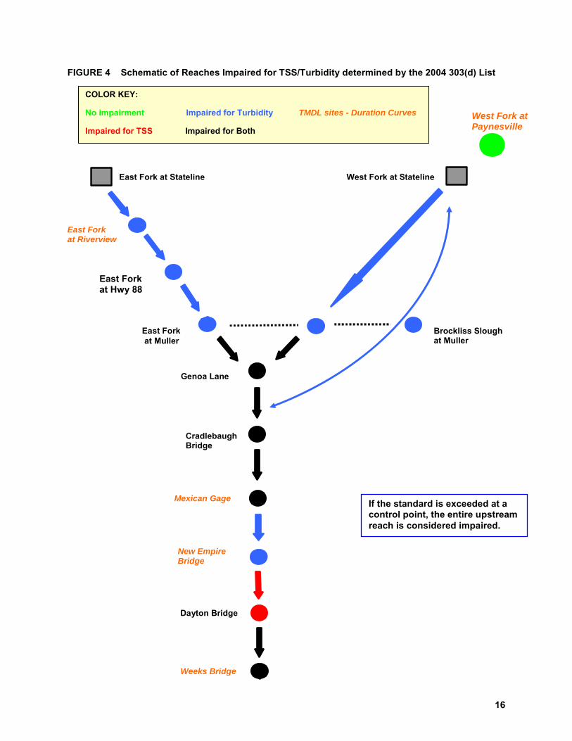
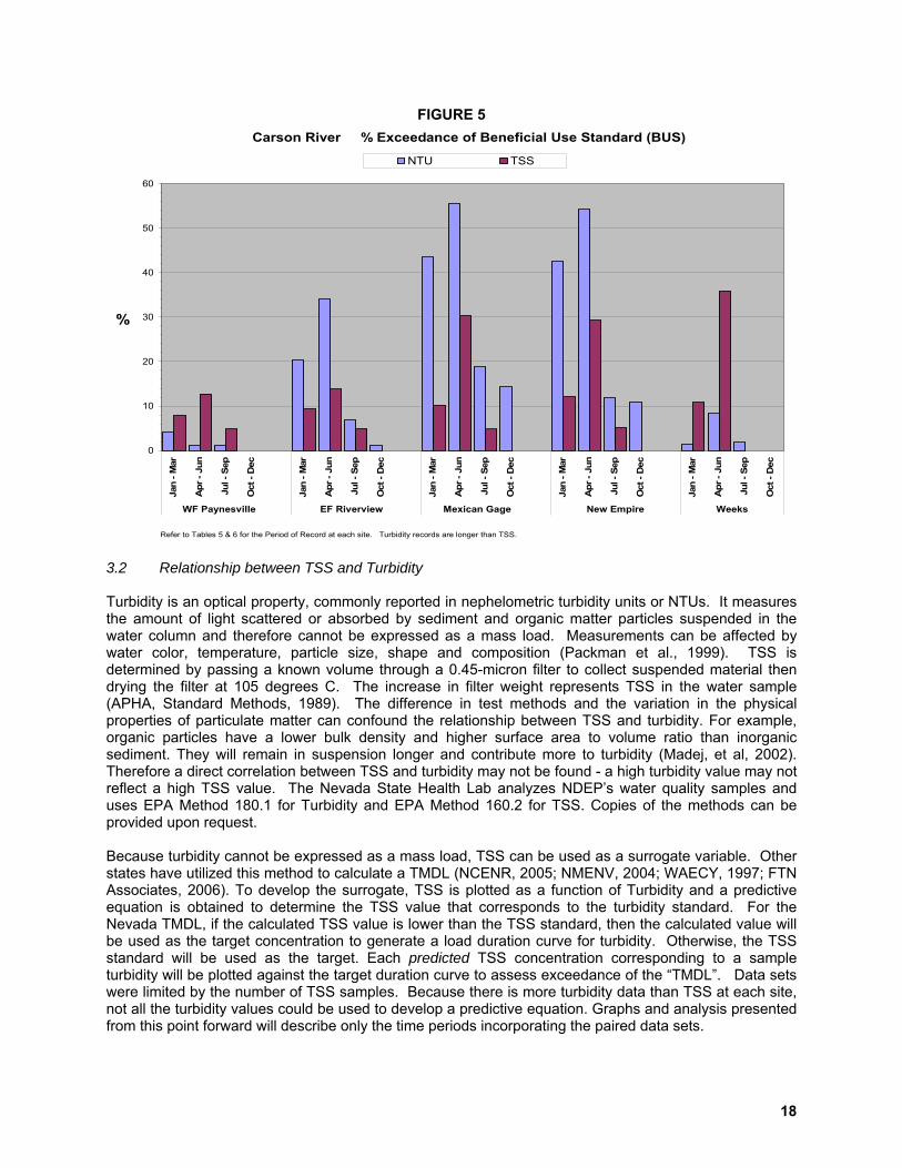
these functions, require costly artificial flood controls to protect new infrastructure and may introduce other water quality problems. According to EPA (1983), copper, lead and zinc were the most prevalent priority pollutants detected in urban runoff. Current water quality samples collected by NDEP now indicate that the West Fork and Main Stem Carson River are exceeding the dissolved zinc standards. However, this may be due to sample contamination. The other two constituents are still below drinking water or aquatic life protection standards. A more comprehensive discussion of the anthropogenic impacts on Carson River geomorphology is presented in the 1996 Inter-Fluve assessment report. The Upper Carson River Watershed Stream Corridor Condition Assessment (2004) sponsored by the Alpine Watershed Group and the Sierra Nevada Alliance, also presents a thorough examination of geomorphic process. These documents are available for review at NDEP. 3.0 Total Suspended Solids and Turbidity TMDLs 3.1 Problem Statement TSS and Turbidity impairment is not consistent along the length of the river (Figure 4). The Carson River is impaired for TSS downstream of Muller Lane on the East and West Forks to the Mexican Gage control point on the Main Stem, therefore requiring development of a “TMDL”. The Carson River from Mexican Gage to New Empire Bridge is not impaired for TSS, but is impaired for TSS from New Empire to Weeks Bridge. The river is impaired for Turbidity from the Stateline on both the East and West Forks to New Empire Bridge; but not from New Empire to Dayton Bridge. Dayton Bridge to Weeks Bridge is impaired for TSS. Figure 4 also depicts where along the river the developed TMDLs will apply. Two TSS TMDLs will be required; four TMDLs for Turbidity. However, load duration curves for both parameters at all 5 sites were generated in order to compare the mass and concentration changes moving down through the system. High concentrations of TSS, which includes inorganic sediment and organic particulates, can be detrimental to aquatic life. Fine sediment can contaminate spawning gravels and cause gill abrasion. Increased turbidity due to high levels of solids increases predation risk and reduces the ability of fish to feed. Increased physiological stress can occur, promoting the susceptibility of fish to disease. For an in-depth review of the effects of turbidity and total suspended solids on salmonids, please refer to Bash, Berman and Bolton (2001). The suspended load also transports adsorbed nutrients or toxic pollutants and can alter stream bed elevation through scour (“hungry” water) and aggradation. Tables 5 and 6 summarize the TSS and Turbidity data as collected by NDEP for the period of record at each “TMDL” site. Mean and median concentrations appear to be increasing downstream to Mexican Gage. Data collected during these longer time periods was used to develop the Target Load Duration Curves rather than the 6 year span used to develop the 2004 303(d) list. Partial data sets were used to construct duration curves for New Empire, because the available flow record (April 1979 - present) at the Deer Run Road gage is shorter than the water quality records. In addition, the gage was not operational from 10/1/85 to 7/30/90. A relatively low number of samples exceed the TSS standards over the period of record at each site. In comparison, greater than 70% of the samples exceeded the Total Phosphorus standard at Mexican Gage, New Empire Bridge and Weeks Bridge (NDEP, 2005). The 2002 and 2004 303(d) lists evaluated 5 and 6 years worth of TSS and Turbidity data respectively. The percent exceedance for Turbidity at Riverview, Mexican Gage and New Empire is greater over the shorter time period (Table 7) compared to the period of record (Table 6). However, the pattern of exceedance is similar - the percent exceedance is greatest at Mexican Gage and New Empire then drops dramatically at Weeks Bridge, because the standard changes from <10 NTU to <50 NTU. Fewer samples are exceeding the standard. Seasonal analysis of the samples violating the standards indicates that the highest percent exceedance (Figure 5) usually occurs during spring runoff (April to June) at each site.

16

FIGURE 4 Schematic of Reaches Impaired for TSS/Turbidity determined by the 2004 303(d) List East Fork at Stateline West Fork at Stateline East Fork at Riverview

Genoa Lane

East Fork at Muller

Cradlebaugh Bridge

Mexican Gage

Dayton Bridge

Weeks Bridge

COLOR KEY: No impairment Impaired for Turbidity TMDL sites - Duration Curves Impaired for TSS Impaired for Both

New Empire Bridge

If the standard is exceeded at a control point, the entire upstream reach is considered impaired.

Brockliss Slough at Muller

West Fork at Paynesville

East Fork at Hwy 88

17

TABLE 5 Summary of Total Suspended Solids Data

Parameter West Fork at Paynesville

East Fork at Riverview

Carson River at Mexican Gage

Carson River at New Empire

Carson River at Weeks

Single Value Standard, mg/L 25 at Stateline 80 80 80 80

Period of Record 2/1980 - 4/2005 11/1978 - 4/2005 2/1980 - 4/2005 11/1978 - 4/2005 3/1985-4/2005

# Samples 233 239 230 238 154

# Samples xcd std 15 17 26 28 19

% Samples xcd std 6.4 7 11 12 12

Average 8 30 42 41 40

Median 6 9 25 18 14

Minimum 0 0 0 1 0

Maximum 94 1012 429 1228 1200

TABLE 6 Summary of Turbidity Data

Parameter West Fork at Paynesville

East Fork at Riverview

Carson River at Mexican Gage

Carson River at New Empire

Carson River at Weeks

Single Value Standard, mg/L ≤10 ≤10 ≤10 ≤10 ≤50

Period of Record 1/1969-4/2005 1/1969-4/2005 9/1975-4/2005 1/1969-4/2005 1/1969-4/2005

# Samples 347 345 264 342 232

# Samples xcd std 6 55 87 104 7

% Samples xcd std 1.7 16 33 30 3

Average 2.1 7 10.4 9.4 12

Median 1.4 3 6.3 6 5

Minimum 0.1 0.2 0.4 0.4 0.1

Maximum 26 180 161 120 436

TABLE 7 %Exceedance of the TSS & Turbidity Standards for the 2002/2004 303(d) Listing Cycles

2002 303(d) List 1997 - 2002 2004 303(d) List 10/1997 - 10/2003 TMDL Site

TSS Turbidity TSS Turbidity

1 West Fork at Paynesville, Ca. 7 7 3 3

2 East Fork at Riverview 7 30 6 21

3 Carson River at Mexican Gage 14 78 11 68

4 Carson River at New Empire 7 70 9 62

5 Carson River at Weeks Bridge 17 11 9* 9*

* Even though the data evaluated dropped below 10% exceedance, there is no evidence that conditions have actually improved for the aquatic life beneficial use; therefore the reaches are still considered impaired. As discussed in Section 2.4, the reduction may simply be an artifact of the amount of data analyzed.

18

FIGURE 5 Carson River % Exceedance of Beneficial Use Standard (BUS)

0

10

20

30

40

50

60Ja

n - M

ar

Apr

- Ju

n

Jul -

Sep

Oct

- D

ec

Jan

- Mar

Apr

- Ju

n

Jul -

Sep

Oct

- D

ec

Jan

- Mar

Apr

- Ju

n

Jul -

Sep

Oct

- D

ec

Jan

- Mar

Apr

- Ju

n

Jul -

Sep

Oct

- D

ec

Jan

- Mar

Apr

- Ju

n

Jul -

Sep

Oct

- D

ec

WF Paynesville EF Riverview Mexican Gage New Empire Weeks

%

NTU TSS

Refer to Tables 5 & 6 for the Period of Record at each site. Turbidity records are longer than TSS. 3.2 Relationship between TSS and Turbidity Turbidity is an optical property, commonly reported in nephelometric turbidity units or NTUs. It measures the amount of light scattered or absorbed by sediment and organic matter particles suspended in the water column and therefore cannot be expressed as a mass load. Measurements can be affected by water color, temperature, particle size, shape and composition (Packman et al., 1999). TSS is determined by passing a known volume through a 0.45-micron filter to collect suspended material then drying the filter at 105 degrees C. The increase in filter weight represents TSS in the water sample (APHA, Standard Methods, 1989). The difference in test methods and the variation in the physical properties of particulate matter can confound the relationship between TSS and turbidity. For example, organic particles have a lower bulk density and higher surface area to volume ratio than inorganic sediment. They will remain in suspension longer and contribute more to turbidity (Madej, et al, 2002). Therefore a direct correlation between TSS and turbidity may not be found - a high turbidity value may not reflect a high TSS value. The Nevada State Health Lab analyzes NDEP’s water quality samples and uses EPA Method 180.1 for Turbidity and EPA Method 160.2 for TSS. Copies of the methods can be provided upon request. Because turbidity cannot be expressed as a mass load, TSS can be used as a surrogate variable. Other states have utilized this method to calculate a TMDL (NCENR, 2005; NMENV, 2004; WAECY, 1997; FTN Associates, 2006). To develop the surrogate, TSS is plotted as a function of Turbidity and a predictive equation is obtained to determine the TSS value that corresponds to the turbidity standard. For the Nevada TMDL, if the calculated TSS value is lower than the TSS standard, then the calculated value will be used as the target concentration to generate a load duration curve for turbidity. Otherwise, the TSS standard will be used as the target. Each predicted TSS concentration corresponding to a sample turbidity will be plotted against the target duration curve to assess exceedance of the “TMDL”. Data sets were limited by the number of TSS samples. Because there is more turbidity data than TSS at each site, not all the turbidity values could be used to develop a predictive equation. Graphs and analysis presented from this point forward will describe only the time periods incorporating the paired data sets.

19

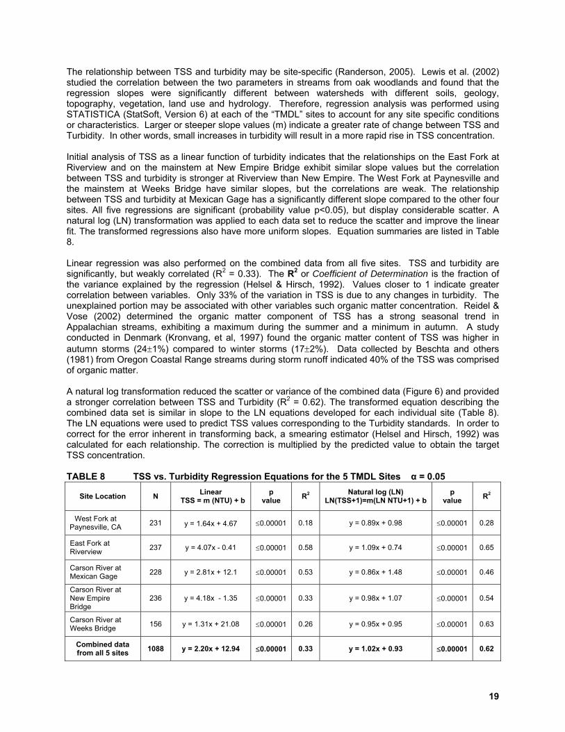
The relationship between TSS and turbidity may be site-specific (Randerson, 2005). Lewis et al. (2002) studied the correlation between the two parameters in streams from oak woodlands and found that the regression slopes were significantly different between watersheds with different soils, geology, topography, vegetation, land use and hydrology. Therefore, regression analysis was performed using STATISTICA (StatSoft, Version 6) at each of the “TMDL” sites to account for any site specific conditions or characteristics. Larger or steeper slope values (m) indicate a greater rate of change between TSS and Turbidity. In other words, small increases in turbidity will result in a more rapid rise in TSS concentration. Initial analysis of TSS as a linear function of turbidity indicates that the relationships on the East Fork at Riverview and on the mainstem at New Empire Bridge exhibit similar slope values but the correlation between TSS and turbidity is stronger at Riverview than New Empire. The West Fork at Paynesville and the mainstem at Weeks Bridge have similar slopes, but the correlations are weak. The relationship between TSS and turbidity at Mexican Gage has a significantly different slope compared to the other four sites. All five regressions are significant (probability value p<0.05), but display considerable scatter. A natural log (LN) transformation was applied to each data set to reduce the scatter and improve the linear fit. The transformed regressions also have more uniform slopes. Equation summaries are listed in Table 8. Linear regression was also performed on the combined data from all five sites. TSS and turbidity are significantly, but weakly correlated (R2 = 0.33). The R2 or Coefficient of Determination is the fraction of the variance explained by the regression (Helsel & Hirsch, 1992). Values closer to 1 indicate greater correlation between variables. Only 33% of the variation in TSS is due to any changes in turbidity. The unexplained portion may be associated with other variables such organic matter concentration. Reidel & Vose (2002) determined the organic matter component of TSS has a strong seasonal trend in Appalachian streams, exhibiting a maximum during the summer and a minimum in autumn. A study conducted in Denmark (Kronvang, et al, 1997) found the organic matter content of TSS was higher in autumn storms (24±1%) compared to winter storms (17±2%). Data collected by Beschta and others (1981) from Oregon Coastal Range streams during storm runoff indicated 40% of the TSS was comprised of organic matter. A natural log transformation reduced the scatter or variance of the combined data (Figure 6) and provided a stronger correlation between TSS and Turbidity (R2 = 0.62). The transformed equation describing the combined data set is similar in slope to the LN equations developed for each individual site (Table 8). The LN equations were used to predict TSS values corresponding to the Turbidity standards. In order to correct for the error inherent in transforming back, a smearing estimator (Helsel and Hirsch, 1992) was calculated for each relationship. The correction is multiplied by the predicted value to obtain the target TSS concentration. TABLE 8 TSS vs. Turbidity Regression Equations for the 5 TMDL Sites α = 0.05

Site Location N Linear TSS = m (NTU) + b

p value R2 Natural log (LN)

LN(TSS+1)=m(LN NTU+1) + b p

value R2

West Fork at Paynesville, CA 231

y = 1.64x + 4.67

≤0.00001 0.18 y = 0.89x + 0.98 ≤0.00001 0.28

East Fork at Riverview 237 y = 4.07x - 0.41 ≤0.00001 0.58 y = 1.09x + 0.74 ≤0.00001 0.65

Carson River at Mexican Gage 228 y = 2.81x + 12.1 ≤0.00001 0.53 y = 0.86x + 1.48 ≤0.00001 0.46

Carson River at New Empire Bridge

236 y = 4.18x - 1.35 ≤0.00001 0.33 y = 0.98x + 1.07 ≤0.00001 0.54

Carson River at Weeks Bridge 156 y = 1.31x + 21.08 ≤0.00001 0.26 y = 0.95x + 0.95 ≤0.00001 0.63

Combined data from all 5 sites 1088 y = 2.20x + 12.94 ≤0.00001 0.33 y = 1.02x + 0.93 ≤0.00001 0.62

20

The corrected surrogate predictions are listed in Table 9 and compared to the TSS standards listed in the NAC. The TSS concentrations corresponding to the Turbidity standards are lower than the TSS standard at Riverview, Mexican Gage and New Empire. The predicted value is higher than the TSS standard at Paynesville and Weeks Bridge. As previously stated, if the calculated TSS value is lower than the TSS standard, then the calculated value will be used as the target concentration to develop a TMDL for Turbidity. If the calculated value is greater than the standard, the original standard will be used to develop the target load duration curve. Because the results from the combined regression are similar to the results obtained by the individual site regressions, the target values calculated from the combined equation were selected to develop the load duration curves. The combined equation was also used to predict TSS concentrations from the sample Turbidity values. Two duration curves have been generated per site to represent the Turbidity and TSS targets. Curves developed for the Paynesville and Weeks Bridge sites will describe both the TSS and Turbidity TMDL.

FIGURE 6 Relationship between Turbidity and TSS

after combining transformed data sets from all 5 TMDL Sites

y = 1.0192x + 0.9324R2 = 0.6149

0.000

1.000

2.000

3.000

4.000

5.000

6.000

7.000

8.000

0.000 1.000 2.000 3.000 4.000 5.000 6.000 7.000

LN NTU+1

LN T

SS+1

TABLE 9 TSS Surrogates corresponding to the Turbidity Standards

Site Turbidity Standard,

NTU

Turbidity Target calculated from Individual Site

regression, mg/L

Turbidity Target calculated from Combined Site

regression, mg/L

TSS Standard,

mg/L

West Fork at Paynesville 10 27 37 25

East Fork at Riverview 10 36 37 80

Carson River at Mexican Gage 10 44 37 80

Carson River at New Empire Bridge 10 39 37 80

Carson River at Weeks Bridge 50 154 183 80

Note: Numbers highlighted in red are the TSS concentrations chosen as load duration curve targets.

21

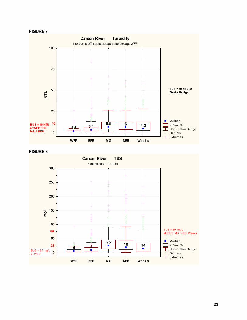
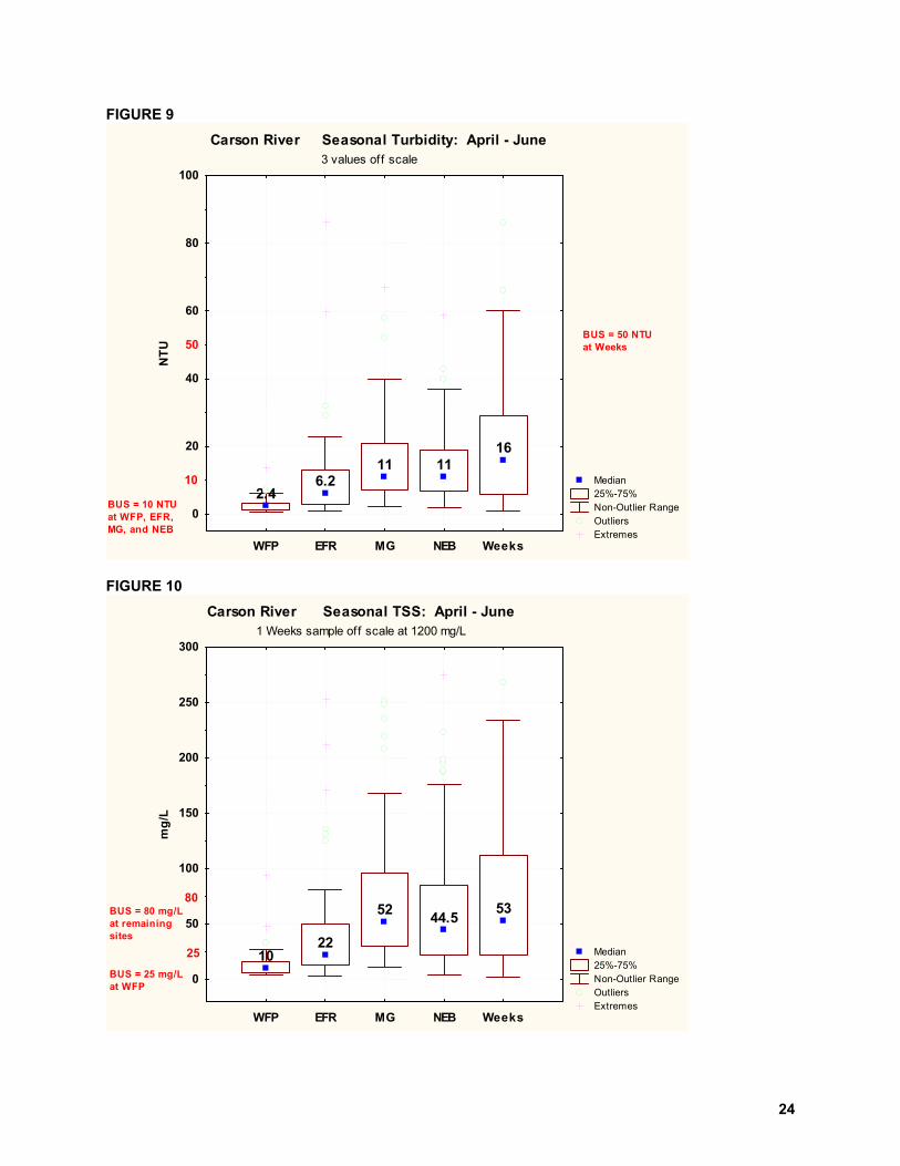
The TSS/Turbidity relationship determined for the West Fork at Paynesville could be considered too weak (R2 = 0.28) to use as a predictive tool. However, TMDLs prepared for Louisiana (USEPA, 2002) and Arkansas (FTN Associates, 2006) use weakly correlated relationships (R2 = 0.34 and 0.30 respectively) to define a Turbidity target. Because the West Fork at Paynesville is not impaired for Turbidity, a TMDL is not required. Surrogate TSS values were still calculated and a load duration curve was constructed for comparison to the downstream sites in Nevada. 3.3 Source Analysis The degraded physical condition of the river system has led to a loss of biological integrity and exceedance of the water quality standards for a number of parameters including TSS, Turbidity, and TP in most Carson River Reaches. Inputs from agricultural return flow, stream bank erosion, sediment stored in the channel, organic matter and urban runoff are all considered potential sources of TSS and Turbidity in the Carson River. Modeling results reported by Carroll et al. (2004) indicate that the flood of 1997 produced 87% of the erosion during the period 1991 to 1997 between Carson City and Fort Churchill. Characterizing the individual TSS or Turbidity sources for allocating loads can be a time and money intensive process; therefore, this TMDL document addresses only general contributions. Box plots (Figures 7 & 8) illustrate the overall change in the distribution of TSS and Turbidity moving downstream for the period of record at each TMDL site and indicate median concentrations are highest at Mexican Gage. These plots provide a simple method to summarize and compare the center, variability and skewness of a data set (Helsel and Hirsch, 1992). Stratifying the data by season indicates a different pattern in transport may be occurring during spring runoff (Figures 9 & 10) compared to the other three time periods. Median concentrations increase between New Empire and Weeks. The overall data distribution for a fewer number of samples is also greater at Weeks than at New Empire, suggesting that streambank erosion is occurring or particulates stored in the channel are being mobilized during spring runoff. Box plots for the other three seasons are provided in Appendix C. The data also indicates that a larger contribution to TSS and turbidity is originating from the East Fork during spring runoff compared to the West Fork. As stated previously in Section 2.5, NDOW (2000) reported that downstream of the town of Minden, sand and silt dominate the substrate on the bottom of the river channel. Pebble count data collected as part of NDEP’s Bioassessment Program supports this observation. The median percentage of substrate determined to be < 2 mm is 67 percent at sites located on the main stem compared to 32 percent at the upstream sites on the East and West Forks. These findings are consistent with field observations and reports from other organizations. Sediment being discharged from land damaged by fire or from erodible, high gradient tributaries to the East Fork in California may be contributing to the suspended solid loads and high turbidity (USFS, 1997). The Upper Carson River Watershed Assessment (2004) prepared for the Alpine Watershed Group and the Sierra Nevada Alliance also report that the East Fork “has significantly higher sediment transport than the West Fork”.

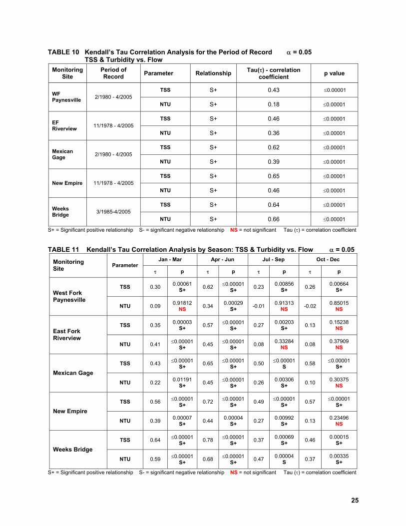
A seasonal evaluation of the period of record data for both TSS and turbidity indicates that the highest median concentrations and loads (Figure 11 & 12) occur April to June during spring runoff at each site, suggesting a correlation with flow. Kendall’s Tau (KT) analysis confirmed flow is significantly correlated with TSS and turbidity for the period of record (Table 10). In addition, TSS is more strongly correlated with flow than turbidity. Breaking down the data by season indicates the strongest correlations occur April to June at each site (Table 11). Kendall Tau correlations are rank-based, appropriate for skewed (non-normal) relationships and were also determined using the STATISTICA software. Strong linear correlations (r > 0.9) correspond to tau values > 0.7 (Helsel & Hirsch, 1992). Relationships that are not significant (p > 0.05) suggest factors other than flow are affecting the concentration. Significant tau values that do not indicate “strong” linear correlations may suggest a nonlinear relationship or indicate other factors are influencing TSS and turbidity in addition to flow, such as particle size. Samples containing the same sediment concentrations but are comprised of different particle sizes can have different turbidity values (Christenson et al, 2002).

22

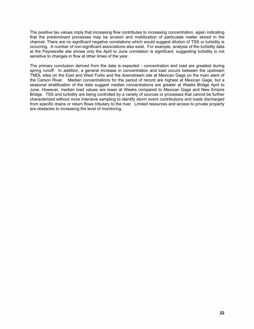
The positive tau values imply that increasing flow contributes to increasing concentration, again indicating that the predominant processes may be erosion and mobilization of particulate matter stored in the channel. There are no significant negative correlations which would suggest dilution of TSS or turbidity is occurring. A number of non-significant associations also exist. For example, analysis of the turbidity data at the Paynesville site shows only the April to June correlation is significant, suggesting turbidity is not sensitive to changes in flow at other times of the year. The primary conclusion derived from the data is expected - concentration and load are greatest during spring runoff. In addition, a general increase in concentration and load occurs between the upstream TMDL sites on the East and West Forks and the downstream site at Mexican Gage on the main stem of the Carson River. Median concentrations for the period of record are highest at Mexican Gage, but a seasonal stratification of the data suggest median concentrations are greater at Weeks Bridge April to June. However, median load values are lower at Weeks compared to Mexican Gage and New Empire Bridge. TSS and turbidity are being controlled by a variety of sources or processes that cannot be further characterized without more intensive sampling to identify storm event contributions and loads discharged from specific drains or return flows tributary to the river. Limited resources and access to private property are obstacles to increasing the level of monitoring.

23

FIGURE 7 Carson River Turbidity

1 extreme off scale at each site except WFPN

TU

Median 25%-75% Non-Outlier Range Outl iers Extremes

1.5 3.16.5 6 4.3

WFP EFR MG NEB Weeks

0

25

50

75

100

BUS = 10 NTU at WFP,EFR, MG & NEB.

BUS = 50 NTU at Weeks Bridge.

10

FIGURE 8

Carson River TSS 7 extremes off scale

Median 25%-75% Non-Outlier Range Outl iers Extremes

6 925 18 14

WFP EFR MG NEB Weeks

0

50

100

150

200

250

300

mg/

L

BUS = 25 mg/L at WFP

BUS = 80 mg/L at EFR, MG, NEB, Weeks

25

80

24

FIGURE 9 Carson River Seasonal Turbidity: April - June

3 values off scale

Median 25%-75% Non-Outlier Range Outliers Extremes

2.46.2

11 1116

WFP EFR MG NEB Weeks

0

20

40

60

80

100N

TU

10

50

BUS = 10 NTU at WFP, EFR, MG, and NEB

BUS = 50 NTU at Weeks

FIGURE 10

Carson River Seasonal TSS: April - June1 Weeks sample off scale at 1200 mg/L

Median 25%-75% Non-Outlier Range Outliers Extremes

1022

52 44.5 53

WFP EFR MG NEB Weeks

0

50

100

150

200

250

300

mg/

L

25BUS = 25 mg/L at WFP

BUS = 80 mg/L at remaining sites

80

25

TABLE 10 Kendall’s Tau Correlation Analysis for the Period of Record α = 0.05 TSS & Turbidity vs. Flow

Monitoring Site

Period of Record Parameter Relationship Tau(τ) - correlation

coefficient p value

TSS S+ 0.43 ≤0.00001 WF Paynesville 2/1980 - 4/2005

NTU S+ 0.18 ≤0.00001

TSS S+ 0.46 ≤0.00001 EF Riverview 11/1978 - 4/2005

NTU S+ 0.36 ≤0.00001

TSS S+ 0.62 ≤0.00001 Mexican Gage 2/1980 - 4/2005

NTU S+ 0.39 ≤0.00001

TSS S+ 0.65 ≤0.00001 New Empire 11/1978 - 4/2005

NTU S+ 0.46 ≤0.00001

TSS S+ 0.64 ≤0.00001 Weeks Bridge 3/1985-4/2005

NTU S+ 0.66 ≤0.00001 S+ = Significant positive relationship S- = significant negative relationship NS = not significant Tau (τ) = correlation coefficient TABLE 11 Kendall’s Tau Correlation Analysis by Season: TSS & Turbidity vs. Flow α = 0.05

Jan - Mar Apr - Jun Jul - Sep Oct - Dec Monitoring Site Parameter

τ p τ p τ p τ p

TSS 0.30 0.00061S+ 0.62 ≤0.00001

S+ 0.23 0.00856 S+ 0.26 0.00664

S+ West Fork Paynesville

NTU 0.09 0.91812 NS 0.34 0.00029

S+ -0.01 0.91313 NS -0.02 0.85015

NS

TSS 0.35 0.00003S+ 0.57 ≤0.00001

S+ 0.27 0.00203 S+ 0.13 0.15238

NS East Fork Riverview

NTU 0.41 ≤0.00001S+ 0.45 ≤0.00001

S+ 0.08 0.33284 NS 0.08 0.37909

NS

TSS 0.43 ≤0.00001S+ 0.65 ≤0.00001

S+ 0.50 ≤0.00001S 0.58 ≤0.00001

S+ Mexican Gage

NTU 0.22 0.01191 S+ 0.45 ≤0.00001

S+ 0.26 0.00306 S+ 0.10 0.30375

NS

TSS 0.56 ≤0.00001S+ 0.72 ≤0.00001

S+ 0.49 ≤0.00001S+ 0.57 ≤0.00001

S+ New Empire

NTU 0.39 0.00007S+ 0.44 0.00004

S+ 0.27 0.00992 S+ 0.13 0.23496

NS

TSS 0.64 ≤0.00001S+ 0.78 ≤0.00001

S+ 0.37 0.00069 S+ 0.46 0.00015

S+ Weeks Bridge

NTU 0.59 ≤0.00001S+ 0.68 ≤0.00001

S+ 0.47 0.00004S 0.37 0.00335

S+

S+ = Significant positive relationship S- = significant negative relationship NS = not significant Tau (τ) = correlation coefficient

26

FIGURE 11

Carson River Seasonal Median Concentrations

0.0

5.0

10.0

15.0

20.0

25.0

30.0

35.0

40.0

45.0

50.0

55.0Ja

n - M

ar

Apr

- Ju

n

Jul -

Sep

Oct

- D

ec

Jan

- Mar

Apr

- Ju

n

Jul -

Sep

Oct

- D

ec

Jan

- Mar

Apr

- Ju

n

Jul -

Sep

Oct

- D

ec

Jan

- Mar

Apr

- Ju

n

Jul -

Sep

Oct

- D

ec

Jan

- Mar

Apr

- Ju

n

Jul -

Sep

Oct

- D

ec

WFP EFR MG NEB Weeks

Feb 80-Apr 05 Nov 78-Apr 05 Feb 80-Apr 05 Nov 78-Apr 05 Mar 85 - Apr 05

mg/

L or

NTU

NTU TSS

FIGURE 12 Carson River Seasonal Median Loads

0

10

20

30

40

50

60

70

80

Jan

- Mar

Apr

- Ju

n

Jul -

Sep

Oct

- D

ec

Jan

- Mar

Apr

- Ju

n

Jul -

Sep

Oct

- D

ec

Jan

- Mar

Apr

- Ju

n

Jul -

Sep

Oct

- D

ec

Jan

- Mar

Apr

- Ju

n

Jul -

Sep

Oct

- D

ec

Jan

- Mar

Apr

- Ju

n

Jul -

Sep

Oct

- D

ec

WF Paynesville EF Riverview Mexican Gage New Empire Weeks

Feb 80-Apr 05 Nov 78-Apr 05 Feb 80-Apr 05 Nov 78-Apr 05 Mar 85 - Apr 05

tons

/day

TSS as surrogate for Turbidity TSS

Note: Values for Jul - Sep Weeks are between 0 & 1 ton/day.

27

3.4 Target Analysis The Carson River TSS and turbidity standards set in the NAC reflect the “desired goal” recommended by EPA in the water quality criteria books to protect propagation of aquatic life. The turbidity standards were used to calculate the surrogate TSS values from the regressions discussed in Section 3.2. For the purposes of this TMDL, the targets have been set at the single value standards listed in Table 9. 3.5 Pollutant Load Capacity and Allocation The TSS Load Capacities or TMDLs for the Carson River are represented by the following equation: TMDL (lbs/day) = Water Quality Target x Flow x 5.39 (Eq. 2) Where: Water quality targets:

o 25 mg/L at West Fork Paynesville for TSS & TSS as a surrogate for Turbidity o 37 mg/L for EF Riverview, Mexican Gage & New Empire for TSS as a surrogate for Turbidity o 80 mg/L at EF Riverview, Mexican Gage & New Empire for TSS o 80 mg/L at Weeks Bridge for TSS & TSS as a surrogate for Turbidity

Flow = streamflow at the appropriate USGS Gage, cfs 5.39 = conversion factor Equation 2 can be illustrated by a load duration curve as described in “Load Duration Curve Methodology for Assessment and TMDL Development” (NDEP, 2003). Under the load duration curve method, water quality data (as a load) are compared to the allowable target loads. Compliance with the TMDLs occurs when 90% of the observed loads fall below the load duration curve. As described in Section 2.2, the Duration Curves are calculated at individual sites, but are applied to the reach upstream of the designated “TMDL” site. Percent contributions from each pollution source have not been determined. A gross load allocation that accounts for all sources of TSS is represented by: Load Allocation (lbs/day) = TMDL (lbs/day) (Eq. 3) As previously discussed, TMDLs should include a margin of safety to account for uncertainties in meeting the water quality standards when the target and TMDL are met. An implicit margin of safety is incorporated in the TSS TMDLs through the conservative assumption that all flow conditions are represented by the load duration curves. The West Fork at Paynesville site is not impaired for TSS or Turbidity and therefore does not require any TMDLs. The East Fork at Riverview is impaired for Turbidity, but not TSS. Load Duration curves were developed for all sites regardless of impairment, in order to illustrate the change in water quality between Carson Valley and the downstream sites. TSS load exceedances based on the period of record are not excessive (Table 12). Surrogate TSS loads have a greater number of exceedances compared to the sample TSS loads because of the lower “standard” at Riverview, Mexican Gage and New Empire determined by the regression analysis. The Watershed Plan developed by the Carson Water Subconservancy District will discuss implementation strategies to reduce the observed pollutant loads in order to meet the TMDLs. Seasonal exceedances for the complete Period of Record at each site are given in Table 13. Target exceedances indicate that an increase in TSS or turbidity is occurring in Carson Valley between the EF and WF sampling sites and the downstream sites at Mexican Gage. The number of exceedances tends to decrease between Mexican and Weeks Bridge, perhaps due to the change in standard or the low gradient in Dayton Valley and subsequent settling of particulates. The TSS as surrogate for turbidity duration curve for the Carson River at Mexican Gage is provided in Figure 13. The curves for the remaining sites are included in Appendix D and E.

28

TABLE 12 % DURATION CURVE EXCEEDANCES for TSS & TURBIDITY FOR THE PERIOD OF RECORD

Site Overall Period of Record Parameter % Exceedance

TSS 6.4 West Fork Paynesville 2/1980 - 4/2005

TSS as NTU* 2.2

TSS 7.1 East Fork Riverview 11/1978 - 4/2005

TSS as NTU 6

TSS 11 Mexican Gage 2/1980 - 4/2005

TSS as NTU 40

TSS 12 New Empire 11/1978 - 4/2005

TSS as NTU 32

TSS 12 Weeks Bridge 3/1985-4/2005

TSS as NTU 12

* TSS as surrogate for Turbidity TABLE 13 % DURATION CURVE EXCEEDANCE BY SEASON

Site Period of Record Parameter Jan - Mar Apr - Jun Jul - Sep Oct - Dec

TSS 8 13 4.8 0 West Fork Paynesville 2/1980 - 4/2005

TSS as NTU* 6 1.8 0 0

TSS 9.4 14 4.8 0 East Fork Riverview 11/1978 - 4/2005

TSS as NTU 17 31 10 0

TSS 10.2 30 4.8 0 Mexican Gage 2/1980 - 4/2005

TSS as NTU 51 66 27 15

TSS 10 30 6.4 0 New Empire 11/1978 - 4/2005

TSS as NTU 41 58.6 13.8 11

TSS 11 36 0 0 Weeks Bridge 3/1985-4/2005

TSS as NTU 13 25.6 5.3 0

* TSS as surrogate for Turbidity Load reductions based on reference conditions are not presented in this TMDL. There is insufficient data to calculate historical loads prior to the degradation that began in the Carson River during the mid 1800’s. Reference reaches have not been established to date because hydrologic alteration and subsequent loss of river function has taken place throughout the Great Basin and it is difficult to identify even the “least disturbed” site on any of the river systems that could be used to determine natural background in the Carson River. Load reduction estimates are determined from the duration curves and will be discussed in the next section.

29

FIGURE 13

3.6 Estimated Load Allocations and Reductions Full compliance with each TMDL occurs when 90% of the observed loads fall below the allowable loads as defined by the Target Duration Curve. Reductions necessary to achieve the TMDL are determined by computing the difference between the median observed sample loads and the corresponding median target loads from the curve for selected duration intervals. The intervals represent the percent of days the load is exceeded under different hydrologic conditions. This method is described for median observed and allowable loads in a white paper written by Tetra Tech (2004). Cleland (2003) also discusses using the duration curve to identify load exceedances under specific conditions. Table 14 provides an example of the calculations at the Mexican Gage control point in Carson City and the data is illustrated in Figure 14. The remaining reduction tables are provided in Appendix G & H. The data demonstrates that most of the sample loads exceeding the targets are concentrated within the 0 to 10% duration interval, which is typically associated with streambank erosion processes. Management of nonpoint source loads produced by extreme flows or flood events, represented by points located on the steepest part of the curve, may not be feasible. Table 15 & 16 shows the influence of spring runoff on loadings within each interval at the “TMDL” sites. The data shows that at each site, > 50% of the loads falling on or above the duration curve within 0-10% exceedance interval were collected in April, May or June. Flows occurring during this time period are dominated by snowmelt. Twenty-eight to fifty percent of loads falling on or above the duration curve within the 10-40% interval were collected in April, May or June.

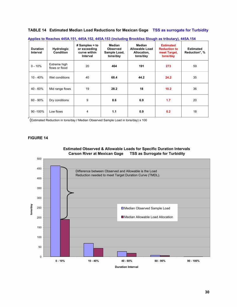
30

TABLE 14 Estimated Median Load Reductions for Mexican Gage TSS as surrogate for Turbidity Applies to Reaches 445A.151, 445A.152, 445A.153 (including Brockliss Slough as tributary), 445A.154

Duration Interval

Hydrologic Condition

# Samples = to or exceeding curve within

Interval

Median Observed

Sample Load, tons/day

Median Allowable Load

Allocation, tons/day

Estimated Reduction to meet Target,

tons/day

Estimated Reduction*, %

0 - 10% Extreme high flows or flood 20 464 191 273 59

10 - 40% Wet conditions 40 68.4 44.2 24.2 35

40 - 60% Mid range flows 19 28.2 18 10.2 36

60 - 90% Dry conditions 9 8.6 6.9 1.7 20

90 -100% Low flows 4 1.1 0.9 0.2 18

* (Estimated Reduction in tons/day / Median Observed Sample Load in tons/day) x 100 FIGURE 14

Estimated Observed & Allowable Loads for Specific Duration IntervalsCarson River at Mexican Gage TSS as Surrogate for Turbidity

0

50

100

150

200

250

300

350

400

450

500

0 - 10% 10 - 40% 40 - 60% 60 - 90% 90 - 100%

Duration Interval

tons

/day

Median Observed Sample Load

Median Allowable Load Allocation

Difference between Observed and Allowable is the Load Reduction needed to meet Target Duration Curve (TMDL).

31

TABLE 15 Percent of April - June Sample Loads Equal to or Exceeding curve within each duration interval TSS

“TMDL” Site Extreme high

flows 0 - 10%

Wet Conditions

10 - 40%

Mid-range flows

40 - 60%

Dry conditions 60 - 90%

Low Flows 90 - 100%

West Fork at Paynesville 58 0 0 0 0

East Fork at Riverview 78 0 0 50 0

Mexican Gage 79 29 0 0 0

New Empire Bridge 71 43 0 0 0

Weeks Bridge 83 57 0 0 0

*TSS as surrogate for Turbidity ** Percentage based on 1 sample. TABLE 16 Percent of April - June Sample Loads Equal to or Exceeding curve

within each duration interval TSS as Surrogate for Turbidity

“TMDL” Site Extreme high

flows 0 - 10%

Wet Conditions

10 - 40%

Mid-range flows

40 - 60%

Dry conditions 60 - 90%

Low Flows 90 - 100%

West Fork at Paynesville 100* 0 0 0 0

East Fork at Riverview 86 28 0 50 0

Mexican Gage 75 50 10 0 0

New Empire Bridge 69 43 31 0 0

Weeks Bridge 64 50 0 0 0

*Percentage based on 1 sample. 3.7 Future Needs The following activities have been identified as critical to further refinement of the TSS and turbidity TMDLs: • Evaluate the water quality data collected by the Conservation Districts and the Desert Research

Institute (DRI) • Assess physical condition and relate characteristics within a reach to the degree of water quality

impairment or biological integrity • Determine if updates to the TSS or turbidity standards are warranted

3.7.1 Supplemental Monitoring Carson Valley and Dayton Valley Conservation Districts conducted additional monitoring with 319 funds to supplement the routine data collected by the state in the Carson River. The programs began in 2002 and ended in December 2005. Samples from the “TMDL” sites will be compared to the developed Duration Curves and NDEP’s ambient data. The additional data may increase the number of duration curve exceedances, because the district monitoring programs target times or flows NDEP does not sample.

32

DRI initiated a continuous turbidity monitoring program in 2002 to obtain a record of magnitude, frequency and duration because the amount of time aquatic life is exposed to particulate matter or sediment is just as important as concentration. Instrumentation was installed at four sites - the East Fork at Riverview, on the West Fork in Diamond Valley, Genoa Lakes Golf Course and downstream of Deer Run Road. Grab samples for TSS are also being collected periodically to establish a relationship between TSS and turbidity. The project was funded with 319/106 monies and a final report is expected by June 2007. 3.7.2 Assessment of Physical Condition Funded through 319 and the CWSD, a Hyperspectral/LiDAR survey was conducted in June 2004 from the California-Nevada state line to Lahontan Reservoir. The information collected may be analyzed to obtain the amount of vegetation or the percentage of incised banks within a specified reach to assess the degree of physical degradation. If resources allow, another survey will be flown in the future to determine changes in system attributes such as vegetation growth in the riparian zone, channel morphology and land use. A comparison between data sets would provide a way to measure river restoration implemented to mitigate nonpoint source pollution and attain the TMDL. Habitat information collected as part of the Bioassessment Program will also be utilized to assess the Carson River. Physical characteristics related to water quality impairment and macroinvertebrate populations will help NDEP establish a clearer picture of overall river health and provide criteria for tracking improvements. Existing conditions will be described in the Carson River watershed assessment or “Report Card”. Projected completion date for this document is December 2007. Linking physical condition to water quality and biology is essential to improving the health of the river system. All stakeholders must work together in a coordinated effort to mitigate the damage caused by hydrogeomorphic alteration and NPS pollution. However, the degree of form and function that can be recreated in a riparian corridor fragmented by urbanization and infrastructure may be minimal because of societal constraints, such as local water law or zoning ordinances. When these constraints restrict restoration activities, stretches of the river that have been rehabilitated are alternated with sections where efforts to revegetate, restore floodplain or mitigate erosion have not occurred. Fragmentation may hinder stakeholder ability to improve water quality and habitat for aquatic life. Localized reaches may be repaired, but because restoration projects are not contiguous, watershed wide improvements may be moderate at best. There must be an understanding that the constraints placed on a river system by the community will limit the extent of restoration and biological function that can be achieved. 3.7.3 Water Quality Standard Updates for TSS and Turbidity Upon completion of the “Report Card”, NDEP will determine if the water quality standards for TSS and turbidity warrant modification to improve support of the beneficial uses. A potential revision may incorporate a duration component. For example, Idaho (IAC, 2006) has established general surface water criteria to protect cold water aquatic life which states “Turbidity, below any applicable mixing zone set by the Department, shall not exceed background by more than 50 NTU instantaneously or 25 NTU for more than 10 consecutive days.” It is also possible that information collected for the watershed assessment (Report Card) may show that other parameters or physical measurements will be a better indicator of river health (e.g. embeddedness, particle size) than TSS or turbidity.

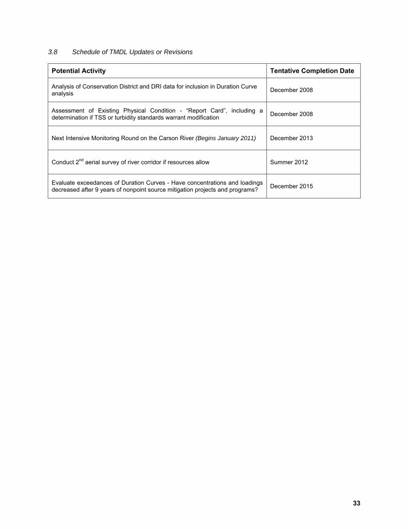
33

3.8 Schedule of TMDL Updates or Revisions

Potential Activity Tentative Completion Date

Analysis of Conservation District and DRI data for inclusion in Duration Curve analysis December 2008

Assessment of Existing Physical Condition - “Report Card”, including a determination if TSS or turbidity standards warrant modification December 2008

Next Intensive Monitoring Round on the Carson River (Begins January 2011) December 2013

Conduct 2nd aerial survey of river corridor if resources allow Summer 2012

Evaluate exceedances of Duration Curves - Have concentrations and loadings decreased after 9 years of nonpoint source mitigation projects and programs? December 2015

34

REFERENCES APHA (American Public Health Association), American Water Works Association, Water Pollution Control Federation, 1989. Standard Methods for the Examination of water and Wastewater, 17th edition. APHA, Washington D.C. Bash, J., Berman, C and Bolton, S, 2001. Effects of Turbidity and Suspended Solids on Salmonids. Prepared by the Center for Streamside Studies, University of Washington and the Washington State Transportation Center for the Washington State Transportation Commission in cooperation with the U.S. Department of Transportation. Beschta, R.L.; O’Leary, S.J.; Edwards, R.E. and Knoop, K.D., 1981. Sediment and organic matter transport in Oregon Coast Range streams. Oregon Water Resources Research Institute, 70. California Department of Water Resources, December 1991. Carson River Atlas. California Department of Fish and Game, Inland Fisheries Division, 1995. Wild Trout Project Spring Newsletter. Retrieved from http://www.dfg.ca.glv/fishing/WildTrout/newsletter.spring95.htm California Department of Fish and Game, 2004. Survey of Fish Populations in Streams of the East Fork Carson River Drainage, California. Fisheries Program Branch Administrative Report No. 2004-8. California Department of Fish and Game, 2004. Survey of Fish Populations in Streams of the East Fork Carson River Drainage, California. Fisheries Program Branch, Administrative Report No. 2004-8. Carroll, R.W.H., Warwick, J.J., James, A.I. and Miller, J.R., 2004. Modeling Erosion and overbank deposition during extreme flood conditions on the Carson River, Nevada. Journal of Hydrology, 297:1-21. Christenson, V.G.; Rasmussen, P.P. and Ziegler, A.C., 2002. Comparison of Estimated Sediment Loads using Continuous Turbidity Measurements and Regression Analysis. Proceedings of Turbidity Workshop, Reno, Nevada, April 30-May 2, 2002. Cleland, Bruce, 2003. TMDL Development from the “Bottom Up” - Part III: Duration Curves and Wet Weather Assessments. America’s Clean Water Foundation. http://www.tmdls.net/tipstools/docs/TMDLsCleland.pdf European Inland Fisheries Advisory Commission (EIFAC), 1965. Water Quality Criteria for European Freshwater Fish: Report on Finely Divided Solids and Inland Fisheries. Journal of Air and Water Pollution. 9:151-168. Federal Interagency Stream Restoration Working Group, 1998. Stream Corridor Restoration: Principles, Processes and Practices. Federal Water Pollution Control Administration, 1968. Water Quality Criteria: Report of the National Technical Advisory Committee to the Secretary of the Interior (The Green Book). FTN Associates, LTD., 2006. TMDLs for Turbidity for Bayou Deview and Cache River, Arkansas. FTN Associates, LTD., 2006. TMDLs for Turbidity for Cadron Creek, Arkansas. Helsel, D.R. and Hirsch, R.M., 1992. Statistical Methods in Water Resources. Elsevier Science Publishers, Amsterdam, the Netherlands.

35

IAC (Idaho Administrative Code), 2006. Department of Environmental Quality, Water Quality Standards, Chapter 58.01.02, Section 250, Surface Water Quality Criteria for Aquatic Life Use Designations, item (e). http://adm.idaho.gov/adminrules/rules/idapa58/0102.pdf Inter-Fluve, Inc., 1996. Fluvial Geomorphic Assessment of the Carson River with Implications for River Management. Kondolf, G. M., 2005. Assessing Long-Term, System-Wide Cumulative Benefits of Multiple Restoration Projects. Eos Trans. AGU. Kronvang, B.; Laubel, A. and Grant, R., 1997. Suspended Sediment and Particulate Phosphorus Transport and Delivery Pathways in an Arable Catchment, GelbaeK Stream, Denmark. Hydrological Processes, 11: 627-642. Lewis, D.J.; Tate, K.W.; Dahlgren, R.A. and Newell, J., 2002. Turbidity and Total Suspended Solid Concentration Dynamics in Streamflow from California Oak Woodland Watersheds. USDA Forest Service General Technical Report, PSW-GTR-184. Madej, Mary Ann; Wilzbach, M.; Cummins, K.; Ellis, C. and Hadden S., 2002. The Contribution of Suspended Organic Sediments to Turbidity and Sediment Flux. Proceedings of Turbidity and Other Sediment Surrogates Workshop, Reno, NV, April 30 - May 2, 2002. National Academy of Sciences and Engineering, 1972. A Report of the Committee on Water Quality Criteria (The Blue Book). Funded by the U.S. Environmental Protection Agency. Newcombe, C.P and MacDonald, D.D., 1991. Effects of Suspended Sediments on Aquatic Ecosystems. North American Journal of Fisheries Management, 11:72-82. Nevada Division of Environmental Protection, April 2003. Load Duration Methodology for Assessment and TMDL Implementation. Nevada Division of Environmental Protection, November 2005. Carson River Phase 1: Total Maximum Daily Loads for Total Phosphorus. Nevada Division of Water Planning, April 1997. Carson River Chronology. Nevada Division of Wildlife, July 1999. Memo from Bob McQuivey, Chief of Habitat to Gene Weller, Chief of Fisheries, Historical Records for the Carson River Fisheries. Nevada Division of Wildlife, May 2000. East Carson River Draft Fisheries Management Plan. NMENV (New Mexico Environment Department), 2004. Total Maximum Daily Load for Turbidity and Stream Bottom Deposits for the Jemez River and the Rio Guadalupe. http://www.nmenv.state.nm.us/swqb/Jemez_Watershed_TMDLs/FINAL-DRAFT-RevisedJemezTurbidityTMDL05-04.pdf NCENR (North Carolina Department of Environment and Natural Resources), Division of Water Quality, 2005. Total Maximum Daily Loads for Turbidity in Long Creek, McAlpine Creek, Sugar Creek, Little Sugar Creek, Irwin Creek, Henry Fork, and Mud Creek in North Carolina. Packman, James J., Comings, Karen J. and Booth, Derek B., 1999. Using Turbidity to Determine Total Suspended Solids in Urbanizing Streams in the Puget Lowlands. Confronting Uncertainty: Managing Change in Water Resources and the Environment, Canadian Water Resources Association annual meeting, Vancouver, BC, p. 158-165.

36

Randerson, T.J., Fink, J.C., Fermanich, K.J., Baumgart, P. and Ehlinger, T., 2005. Total Suspended Solids - Turbidity Correlation in Northwestern Wisconsin Streams. AWRA Section Meeting, Delavan Wisconsin. http://www.uwgb.edu/watershed/student/activities/Presentations/AWRA_Randerson.pdf Riedel, Mark S. and Vose, James M., 2002. The dynamic nature of sediment and organic constituents in TSS. Proc. 2002 National Monitoring Conference, National Water Quality Monitoring Council, May 20 - 23, Madison, Wisconsin. http://www.srs.fs.usda.gov/pubs/ja/ja_riedel001.pdf Tetra Tech, Inc., 2004. White Paper (l): Advantages and Disadvantages of Using Load Duration Curves to Estimate Existing and Allowable Loads for the Development of Nutrient TMDLs. http://rd.tetratech.com/epa/ U.S. Environmental Protection Agency, 1983. Results of the Nationwide Urban Runoff Program. Volume 1-Final Report. Office of Water, Washington, D.C. U.S. Environmental Protection Agency, April 1991. Guidance for Water Quality Based Decisions-The TMDL Process (EPA 440/4-91-001). U.S. Environmental Protection Agency, October 1999. Protocol for Developing Sediment TMDLs EPA 841-B-99-004).

U.S. Environmental Protection Agency, Region VI, May 2002. Total Maximum Daily Load for Suspended Solids and Turbidity for English Bayou (subsegment 030702) in the Calcasieu River Basin (Louisiana). U.S. Environmental Protection Agency, Federal Register, 10/23/03. Nonpoint Source Program and Grants Guidelines for States and Territories. http://www.epa.gov/owow/nps/cwact.html U.S. Forest Service, 1997. Silver Creek Area Analysis, Humboldt-Toiyabe National Forest, Alpine County, California. Upper Carson River Watershed Stream Corridor Condition Assessment, 2004. Prepared for the Alpine Watershed Group and Sierra Nevada Alliance by MACTEC Engineering and Consulting, Swanson Hydrology and Geomorphology, River Run Consulting and C.G. Celio and Sons. WAECY (Washington State Department of Ecology), 1997. A Suspended Sediment and DDT Total Maximum Daily Load Evaluation Report for the Yakima River.

37

APPENDIX A Monthly Mean Flows for Selected Gaging Stations

Mean Monthly Streamflow (1901-2005) West Fork Carson River at Woodfords, CA USGS #10310000

0

50

100

150

200

250

300

350

400

Oct Nov Dec Jan Feb Mar Apr May Jun Jul Aug Sep

cfs

Mean Monthly Streamflow (1940-2005) Carson River near Carson City, NV USGS #10311000

0

200

400

600

800

1000

1200

1400

Oct Nov Dec Jan Feb Mar Apr May Jun Jul Aug Sep

cfs

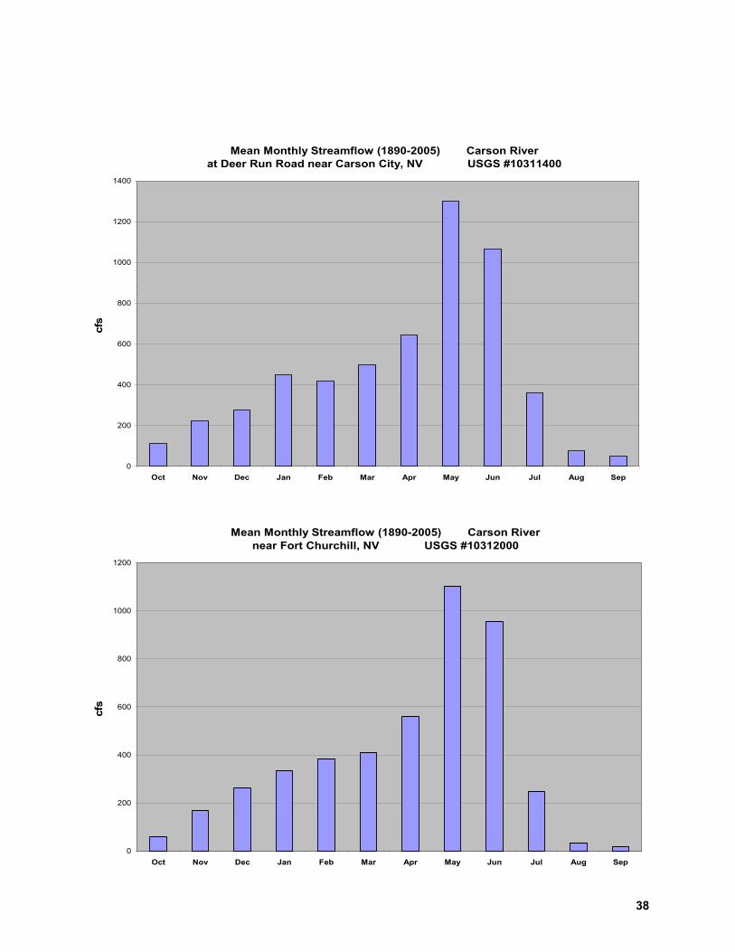
38

Mean Monthly Streamflow (1890-2005) Carson River at Deer Run Road near Carson City, NV USGS #10311400

0

200

400

600

800

1000

1200

1400

Oct Nov Dec Jan Feb Mar Apr May Jun Jul Aug Sep

cfs

Mean Monthly Streamflow (1890-2005) Carson River

near Fort Churchill, NV USGS #10312000

0

200

400

600

800

1000

1200

Oct Nov Dec Jan Feb Mar Apr May Jun Jul Aug Sep

cfs

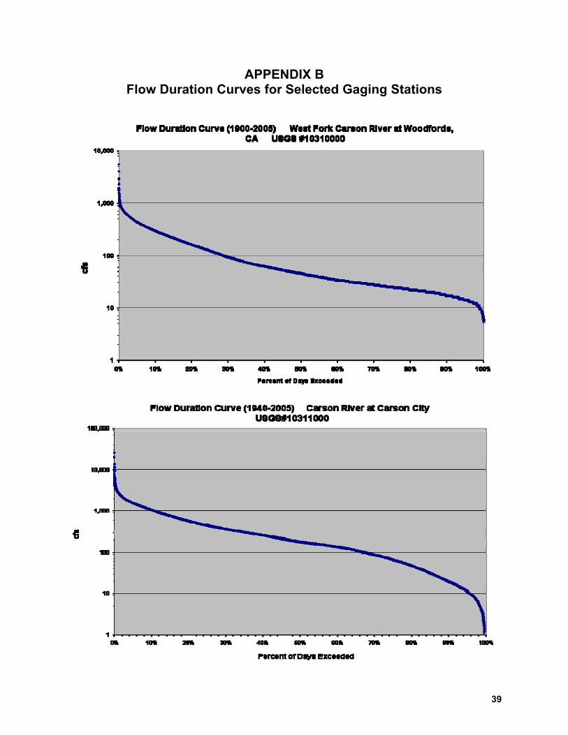
39

APPENDIX B Flow Duration Curves for Selected Gaging Stations

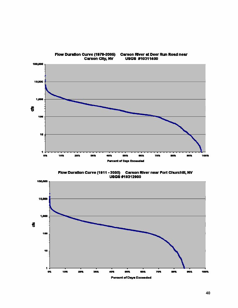
40

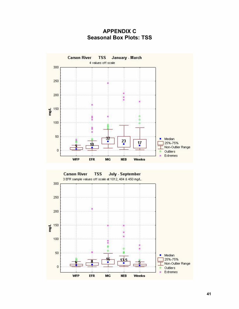
41

APPENDIX C Seasonal Box Plots: TSS

42

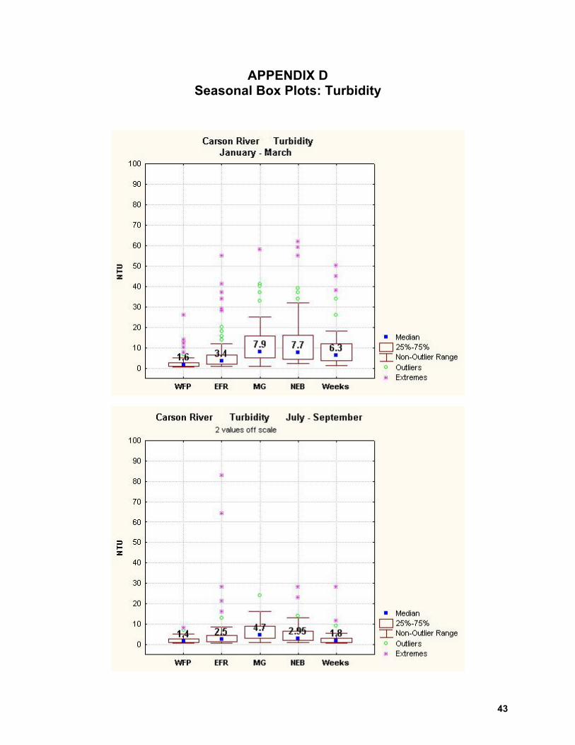
43

APPENDIX D Seasonal Box Plots: Turbidity

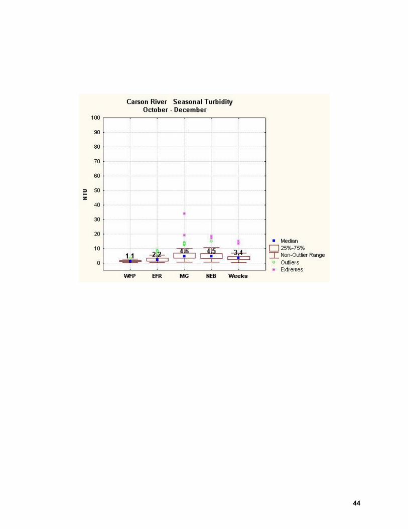
44

45

APPENDIX E Load Duration Curves: TSS

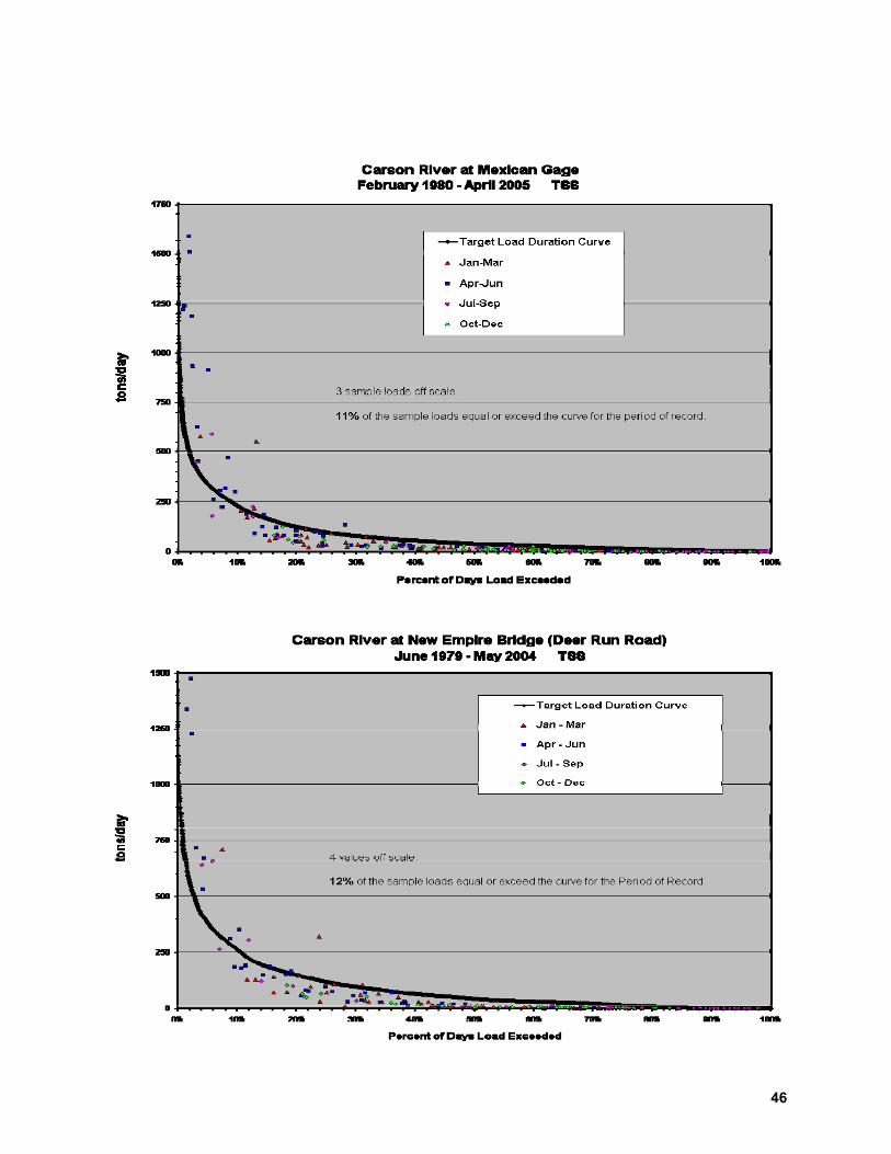
46

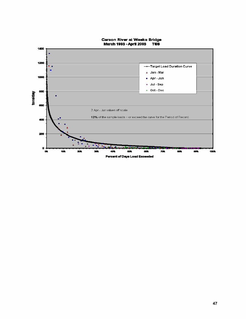
47

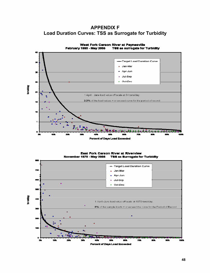
48

APPENDIX F Load Duration Curves: TSS as Surrogate for Turbidity

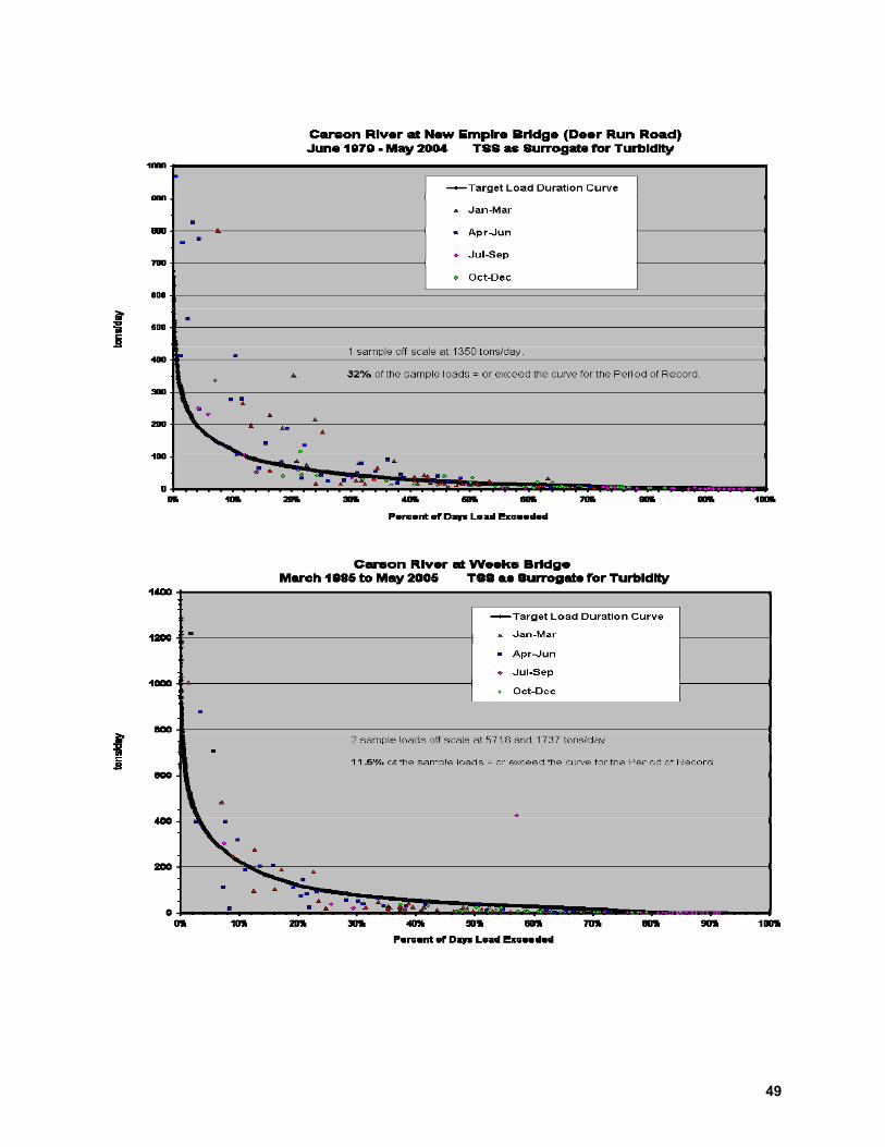
49

50

APPENDIX G Load Reduction Estimates for TSS

West Fork Paynesville Not impaired for TSS

Duration Interval

Hydrologic Condition

# Samples = to or exceeding curve within

Interval

Median Observed

Sample Load, tons/day

Median Allowable

Load Allocation, tons/day

Estimated Reduction to meet Target,

tons/day

Estimated Reduction*, %

0 - 10% Extreme high flows or flood 12 47.8 40 7.8 16

10 - 40% Wet conditions 0 0 0 0 0

40 - 60% Mid range flows 1 4 3.4 0.6 15

60 - 90% Dry conditions 1 2.1 1.6 0.5 24

90 - 100% Low flows 1 0.98 0.94 0.04 4

* (Estimated Reduction in tons/day / Median Observed Sample Load in tons/day) x 100 East Fork Riverview Not impaired for TSS

Duration Interval

Hydrologic Condition

# Samples = to or exceeding curve within

Interval

Median Observed

Sample Load, tons/day

Median Allowable

Load Allocation, tons/day

Estimated Reduction to meet Target,

tons/day

Estimated Reduction*, %

0 - 10% Extreme high flows or flood 9 997 431 566 57

10 - 40% Wet conditions 6 259 128 131 51

40 - 60% Mid range flows 0 0 0 0 0

60 - 90% Dry conditions 2 85 22 63 74

90 - 100% Low flows 0 0 0 0 0

* (Estimated Reduction in tons/day / Median Observed Sample Load in tons/day) x 100

Mexican Gage Applies to Reaches 445A.152, 445A.153 (including Brockliss S. as Tributary) and 445A.154

Duration Interval

Hydrologic Condition

# Samples = to or exceeding curve within

Interval

Median Observed

Sample Load, tons/day

Median Allowable Load

Allocation, tons/day

Estimated Reduction to meet Target,

tons/day

Estimated Reduction*, %

0 - 10% Extreme high flows or flood 19 915 418 497 54

10 - 40% Wet conditions 7 185 170 15 8

40 - 60% Mid range flows 0 0 0 0 0

60 - 90% Dry conditions 0 0 0 0 0

90 - 100% Low flows 0 0 0 0 0

* (Estimated Reduction in tons/day / Median Observed Sample Load in tons/day) x 100

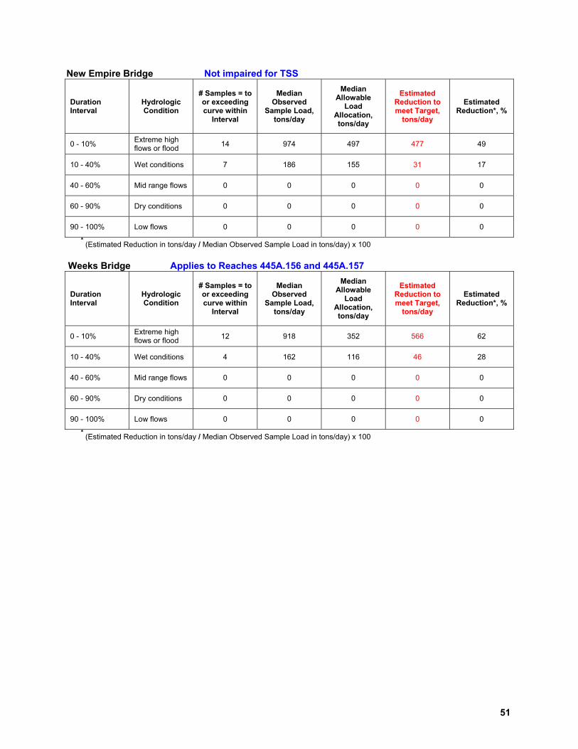
51

New Empire Bridge Not impaired for TSS

Duration Interval

Hydrologic Condition

# Samples = to or exceeding curve within

Interval

Median Observed

Sample Load, tons/day

Median Allowable

Load Allocation, tons/day

Estimated Reduction to meet Target,

tons/day

Estimated Reduction*, %

0 - 10% Extreme high flows or flood 14 974 497 477 49

10 - 40% Wet conditions 7 186 155 31 17

40 - 60% Mid range flows 0 0 0 0 0

60 - 90% Dry conditions 0 0 0 0 0

90 - 100% Low flows 0 0 0 0 0

* (Estimated Reduction in tons/day / Median Observed Sample Load in tons/day) x 100 Weeks Bridge Applies to Reaches 445A.156 and 445A.157

Duration Interval

Hydrologic Condition

# Samples = to or exceeding curve within

Interval

Median Observed

Sample Load, tons/day

Median Allowable

Load Allocation, tons/day

Estimated Reduction to meet Target,

tons/day

Estimated Reduction*, %

0 - 10% Extreme high flows or flood 12 918 352 566 62

10 - 40% Wet conditions 4 162 116 46 28

40 - 60% Mid range flows 0 0 0 0 0

60 - 90% Dry conditions 0 0 0 0 0

90 - 100% Low flows 0 0 0 0 0

* (Estimated Reduction in tons/day / Median Observed Sample Load in tons/day) x 100

52

APPENDIX H Load Reduction Estimates for TSS as a Surrogate for Turbidity

West Fork Paynesville Not impaired for Turbidity

Duration Interval

Hydrologic Condition

# Samples = to or exceeding curve within

Interval

Median Observed

Sample Load, tons/day

Median Allowable

Load Allocation, tons/day

Estimated Reduction to meet Target,

tons/day

Estimated Reduction*, %

0 - 10% Extreme high flows or flood 1 84 59 25 30

10 - 40% Wet conditions 3 8.2 6.9 1.3 16

40 - 60% Mid range flows 0 0 0 0 0

60 - 90% Dry conditions 1 2.6 1.8 0.8 31

90 - 100% Low flows 0 0 0 0 0

* (Estimated Reduction in tons/day / Median Observed Sample Load in tons/day) x 100 East Fork Riverview Applies to Reach 445A.150 only

Duration Interval

Hydrologic Condition

# Samples = to or exceeding curve within

Interval

Median Observed

Sample Load, tons/day

Median Allowable

Load Allocation, tons/day

Estimated Reduction to meet Target,

tons/day

Estimated Reduction*, %

0 - 10% Extreme high flows or flood 14 448 173 275 61

10 - 40% Wet conditions 18 135 59 76 56

40 - 60% Mid range flows 0 0 0 0 0

60 - 90% Dry conditions 2 118 9.4 108.6 92

90 - 100% Low flows 1 9 6 3 33

* (Estimated Reduction in tons/day / Median Observed Sample Load in tons/day) x 100

New Empire Bridge Applies to Reach 445A.155

Duration Interval

Hydrologic Condition

# Samples = to or exceeding curve within

Interval

Median Observed

Sample Load, tons/day

Median Allowable

Load Allocation, tons/day

Estimated Reduction to meet Target,

tons/day

Estimated Reduction*, %

0 - 10% Extreme high flows or flood 16 644 204 440 68

10 - 40% Wet conditions 28 111 62 49 44

40 - 60% Mid range flows 13 34 24 10 29

60 - 90% Dry conditions 5 19 12.7 6.3 33

90 - 100% Low flows 1 1 0.9 0.1 10

* (Estimated Reduction in tons/day / Median Observed Sample Load in tons/day) x 100

53

Weeks Bridge Applies to Reach 445A.157 only

Duration Interval

Hydrologic Condition

# Samples = to or exceeding curve within

Interval

Median Observed

Sample Load, tons/day

Median Allowable

Load Allocation, tons/day

Estimated Reduction to meet Target,

tons/day

Estimated Reduction*, %

0 - 10% Extreme high flows or flood 11 702 311 391 56

10 - 40% Wet conditions 6 195 148 47 24

40 - 60% Mid range flows 1 426 29 397 93

60 - 90% Dry conditions 0 0 0 0 0

90 - 100% Low flows 0 0 0 0 0

* (Estimated Reduction in tons/day / Median Observed Sample Load in tons/day) x 100