Ocean Modelling 32 (2010) 157–169

Contents lists available at ScienceDirect

Ocean Modelling

journal homepage: www.elsevier .com/locate /ocemod

Total kinetic energy in four global eddying ocean circulation models and over5000 current meter records

Robert B. Scott a,c,*, Brian K. Arbic b, Eric P. Chassignet b, Andrew C. Coward c, Mathew Maltrud d,William J. Merryfield e, Ashwanth Srinivasan f, Anson Varghese a

a Institute for Geophysics, Jackson School of Geosciences, The University of Texas at Austin, J.J. Pickle Research Campus, Bldg. 196 (ROC), 10100 Burnet Rd. (R2200),Austin, TX 78759, United Statesb Department of Oceanography and Center for Ocean-Atmospheric Prediction Studies, The Florida State University, Tallahassee, FL 32306, United Statesc James Rennell Division for Ocean Circulation and Climate, National Oceanography Centre, Southampton, Southampton SO14 3ZH, United Kingdomd Climate, Ocean and Sea Ice Modeling Project, Fluid Dynamics Group, Los Alamos National Laboratory, Los Alamos, NM 87545, United Statese Canadian Centre for Climate Modelling and Analysis, Meteorological Service of Canada, University of Victoria, P.O. Box 1700, Victoria, BC, Canada V8W 2Y2f RSMAS/MPO and Center for Computational Science, University of Miami, Miami, FL, United States

a r t i c l e i n f o a b s t r a c t

Article history:Received 14 July 2009Received in revised form 17 December 2009Accepted 20 January 2010Available online 1 February 2010

Keywords:Eddying OGCMKinetic energyMoored current metersModel validationModel intercomparison

1463-5003/$ - see front matter � 2010 Elsevier Ltd. Adoi:10.1016/j.ocemod.2010.01.005

* Corresponding author. Address: Institute for GeGeosciences, The University of Texas at Austin, J.J. P196 (ROC), 10100 Burnet Rd. (R2200), Austin, TX 7875471 0375; fax: +1 512 471 8844.

E-mail address: rscott@ig.utexas.edu (R.B. Scott).

We compare the total kinetic energy (TKE) in four global eddying ocean circulation simulations with aglobal dataset of over 5000, quality controlled, moored current meter records. At individual mooringsites, there was considerable scatter between models and observations that was greater than estimatedstatistical uncertainty. Averaging over all current meter records in various depth ranges, all four modelshad mean TKE within a factor of two of observations above 3500 m, and within a factor of three below3500 m. With the exception of observations between 20 and 100 m, the models tended to straddle theobservations. However, individual models had clear biases. The free running (no data assimilation) modelbiases were largest below 2000 m. Idealized simulations revealed that the parameterized bottom bound-ary layer tidal currents were not likely the source of the problem, but that reducing quadratic bottomdrag coefficient may improve the fit with deep observations. Data assimilation clearly improved themodel-observation comparison, especially below 2000 m, despite assimilated data existing mostly abovethis depth and only south of 47 �N. Different diagnostics revealed different aspects of the comparison,though in general the models appeared to be in an eddying-regime with TKE that compared reasonablywell with observations.

� 2010 Elsevier Ltd. All rights reserved.

1. Introduction

In the current decade several global ocean general circulationmodels, OGCMs, have been run in the eddying-regime; for a reviewof the state-of-the-art, see the collection of papers edited by Hechtand Hasumi (2008). Since we expect the processes generatingmesoscale variability are now, at least potentially, well repre-sented by the discrete formulations of the governing equations,the question of how well the simulated mesoscale currents com-pare with observations becomes increasingly important. Becausethe mesoscale velocity field is observed to be highly variable andbelieved to be strongly turbulent, we can only hope to comparestatistical properties of the mesoscale velocity field, such as the

ll rights reserved.

ophysics, Jackson School ofickle Research Campus, Bldg.9, United States. Tel.: +1 512

total kinetic energy (TKE) level and the zonal and meridional meansquared velocities. The equilibrated TKE will be a balance betweengeneration, nonlinear redistribution in physical space, and dissipa-tion. Dissipation is likely the most unreliable modeled process be-cause it must be approximated with ad hoc parameterization of theinteraction with subgrid scale flows both at the boundaries andthroughout the interior of the ocean.

Many studies have compared OGCM surface kinetic energy, orsea level height anomaly variability, with observations from satel-lite-based radar altimeters, and most OGCMs with resolution about1/6� or better compare quite favorably over most of the WorldOcean (e.g. Paiva et al., 1999; Smith et al., 2000; Hurlburt andHogan, 2000; Maltrud and McClean, 2005; Barnier et al., 2006;Chassignet et al., 2009). Less is known about the deeper ocean ki-netic energy, though high-resolution North Atlantic simulationswith a hydrodynamic six-layer model, NLOM (Naval Research Lab-oratory Layered Ocean Model), suggested that model grid resolu-tion as high as about 1/32� may be necessary to obtainconvergence of the abyssal kinetic energy (Hurlburt and Hogan,

Table 1Models analyzed in this study. FR = free running (no data assimilation); DA = dataassimilation; B = Boussinesq; NB = non-Boussinesq; PE = primitive eqns.; Cd = qua-dratic drag coefficient; UT = tidal speed.

Quantity OCCAM POP HYCOM FR HYCOM DA

Equations B, PE B, PE NB, PE NB, PE, DAVert. coord. Z Z q;Z;r q;Z;rVert. res. 66 levels 42 levels 32 layers 32 layersHoriz. res. 1/12� lon-lat 1/10�lon 1/12� lon 1/12� lonCd 0.001 0.001 0.0022 0.0022UT 5 cm/s 0 5 cm/s 5 cm/sOutput 5-day mean Daily mean Daily snapshot Daily snapshot

158 R.B. Scott et al. / Ocean Modelling 32 (2010) 157–169

2000). Because of the poor vertical resolution of the NLOM model,and the unusual compression of topography employed, it is diffi-cult to extrapolate these results to other models. But at the veryleast this study alerts us to the possibility that resolution muchhigher than the first baroclinic mode Rossby radius of deformationmight be required to obtain realistic subsurface flows, see discus-sion by Treguier (2006).

In contrast with the wealth of observational information avail-able at the ocean surface, subsurface data are much more limited,and more cumbersome to work with. While some Lagrangian dataare available from subsurface floats, Eulerian data are morestraightforward to analyze so we have focused on moored currentmeters. The most comprehensive comparison of OGCM andmoored current meter kinetic energy throughout the water columnhas been by Penduff et al. (2006). They compared 891 Atlantic cur-rent meter records from the World Ocean Circulation Experiment(WOCE) with the 1/6� CLIPPER Atlantic OGCM. They found themodel currents tend to be too baroclinic (too vertically sheared,so they are increasingly too weak at greater depths). This suggeststhat even if OGCMs compare well with surface observations,important model biases may remain at depth. This concern wassubstantiated by Arbic et al. (2009), who compared the abyssalflows in two versions of NLOM and global 1/10� POP (ParallelOcean Program) with a superset of the WOCE current meter data-base, maintained by Oregon State University. They found that thepoint-by-point comparison of time-averaged cube of bottom flowspeeds1 in models and current meters was poor (there was a greatdeal of scatter in the scatterplots). When the time-averages werethen averaged over many mooring sites, the models performed bet-ter (within a factor of 2.7 or less for the cube of bottom flow), butstill displayed a bias toward weak flow, as found by Penduff et al.(2006). The present study is more comprehensive than these twoearlier studies, in that we will undertake comparisons both through-out the full-water column (as done by Penduff et al., 2006), andthroughout the globe (as done by Arbic et al., 2009).

There is some suggestion that the present generation globaleddying models should be able to produce realistic energy levels,and vertical structure of currents. Evidence in support of a realisticvertical structure of the currents in a 1/10� North Atlantic POP sim-ulation is provided by Smith et al. (2000, Fig. 8), showing goodagreement between baroclinic, barotropic and total Gulf Streamtransports with those from current meter moorings by Hogg(1992) and Johns et al. (1995). Further evidence is provided bycomparison with eddy kinetic energy (EKE) from moored currentmeters along 48 �N (Colin de Verdiere et al., 1989), see Smithet al. (2000, Fig. 16). Note in particular the strong EKE at depthsgreater than 1000 m along 35 �W, with values between about 25and 44 cm2/s2 in the mooring, which corresponds well with about50 cm2/s2 in the model.

There are now several global OGCMs run in a realistic configu-ration with horizontal resolution of 1/10� to 1/12� (see Table 1),which resolve the first Rossby radius of deformation throughoutmost of the domain (i.e. up to �55 �N) and are able to have a goodrepresentation of upper ocean baroclinic processes. How well dothese models simulate TKE throughout the full extent of the watercolumn? Is resolution the only factor that determines a model’ssuccess? The global models in Table 1 have comparable resolutionto the 1/10� North Atlantic POP model, but vary in their numericalformulation. In particular, POP and OCCAM are Arakawa B-gridmodels with geopotential (z-level) vertical coordinate, while HY-COM uses the Arakawa C-grid and hybrid vertical coordinates.We have analyzed the free-running versions of all three models,

1 Arbic et al. (2009) analyzed the cube of the speed because bottom boundary layerdissipation rate is proportional to this.

as well as the data assimilative version of HYCOM. The globaleddying OGCMs analyzed in this study are described in further de-tail in Appendix B. The present study aims to assess the ability ofthese models to simulate realistic zonal and meridional TKE. Thiswill be assessed using a large, moored current meter, archive(CMA). Section 2 introduces the CMA compiled for this study, thequality control applied, and the data processing steps, with furtherdetails in Appendix A. Section 3 describes briefly the OGCM outputpreprocessing. Section 4 presents the comparison of OGCMs andthe CMA. In Section 5 we include a set of experiments using ideal-ized MOM4 simulations to quantify the role of bottom frictionparameters. We conclude with a discussion and summary of thekey findings in Section 6.

2. Moored current meter records

2.1. Multiarchive current meter dataset

The Current Meter Archive was created by combining the DeepWater Archive of the Oregon State University (OSU) Buoy Group,1901 current meter records collected by Carl Wunsch, and othersources. The current meter records were between September1973 and February 2005. The OSU dataset contains over 5000 cur-rent meter records (including acoustic and mechanical devices, onsurface and subsurface moorings) from many investigators and in-cludes the WOCE archive. Most records are in deep water and typ-ically have at least 6-month duration. Each record was visuallyinspected and quality controlled by the OSU Buoy Group as de-scribed on their website http://kepler.oce.orst.edu/. The recordswere checked for typical problems such as stalled rotors or stickingcompass, fouling of speed sensors, tape glitches, etc. Problemswere removed and gaps less than about a week long were filledin with predictive interpolation, a maximum entropy method de-signed to produce less distortion to the power spectrum than sim-ple linear interpolation. Longer stretches of suspect data wereflagged as missing. Further details can be found on the OSU BuoyGroup webpage.

The archive provided by Carl Wunsch contained 1901 recordson 525 moorings, of which over 100 moorings were visually in-spected (Wunsch, pers. comm. 2009) and analyzed by Wunsch(1997). Literature citations to the first published work on the var-ious moorings were tabulated by Wunsch (1997). The records werefurther quality controlled for the present study by visual inspec-tions and comparing with records that also appeared in the OSUdataset. Some outliers were identified through comparison withthe models in the current study, and problems traced to varioussources such as units errors.

We also obtained 59 current meter records from several exper-iments in the online archive maintained by the Upper Ocean Pro-cesses Group at Woods Hole Oceanographic Institution, http://uop.whoi.edu/index.html.

We searched for redundancies with the following chosen toler-ances for deciding if records were co-located: 0.005� latitude and

R.B. Scott et al. / Ocean Modelling 32 (2010) 157–169 159

longitude, and 5 cm in the vertical. This revealed over 500 redun-dant records, though more redundancies could be found with lessstrict tolerances. Records overlapping in time were dealt withwhen computing the mean statistics.

Our CMA and the software interface are described at http://www.ig.utexas.edu/research/projects/cma/data.html, and are avail-able upon request.

2.2. Data selection and preprocessing

We found 5814 unique current meter records that were mooredin more than 10 m of water, and had more than 90 days of gooddata. These 5814 records were further checked with automatedroutines for problems such as rotor or vane being stuck, or suspi-cious gaps in the data. This was accomplished by dividing eachtime series into sections of at least 10 days of consecutive points(or at least 30 points for records with sampling period greater than8 h) and checking if the standard deviation of either u;v , or speedwas less than 5� 10�4 m/s, or the standard deviation of directionwas less than 0.05�. This identified a further 46 records as suspect.Reducing the threshold by �5 (less strict) yielded 40 bad records.However, doubling the time window to 20 days cut the rejected re-cords to only 23, so there remains some inevitable arbitrariness inchoosing tolerances. After these quality control steps, there re-mained 5741 records on 1363 mooring locations. Sampling fre-quencies varied from 8 min to 1 day, so many records containedstrong tidal and near inertial gravity wave components. To producehomogeneous records for comparison with mesoscale motionssimulated in the OGCMs, the current meter ðu;vÞ time series werereduced to 5-day averages. Records with missing data in a 5-dayperiod were averaged over available good data if at least 5/2 daysof good data were available; otherwise that time period wasflagged as missing. No temporal interpolation was performed.Applying a 3-day Butterworth filter to the records to more cleanlyremove the tidal and other high-frequency signals prior to taking5-day averages led to negligible differences.

The POP model was compared with an earlier version of theCMA (CMA 1.0) containing only 1198 moorings of the 1363 con-tained in the current version (CMA 2.0). All other models werecompared with the 1363 mooring database. Evaluating HYCOMand OCCAM with CMA 1.0 instead of CMA 2.0 led to changes inthe correlation coefficients (Table 2) of at most 0.01, and scatter-plots were visually indistinguishable from those presented.

At some locations current meter moorings were re-deployed atthe same location and depth multiple times. From the 5741 qualitycontrolled current meter records we found 5339 unique depth binswith at least 90-days of accumulated 5-day averaged velocities, on1361 mooring sites. Hereafter, we will refer to these as ‘‘records”even though they were actually combinations of current meterrecords deployed at very similar locations and depths at differentdates, often with considerable temporal gap. There were 4466 re-

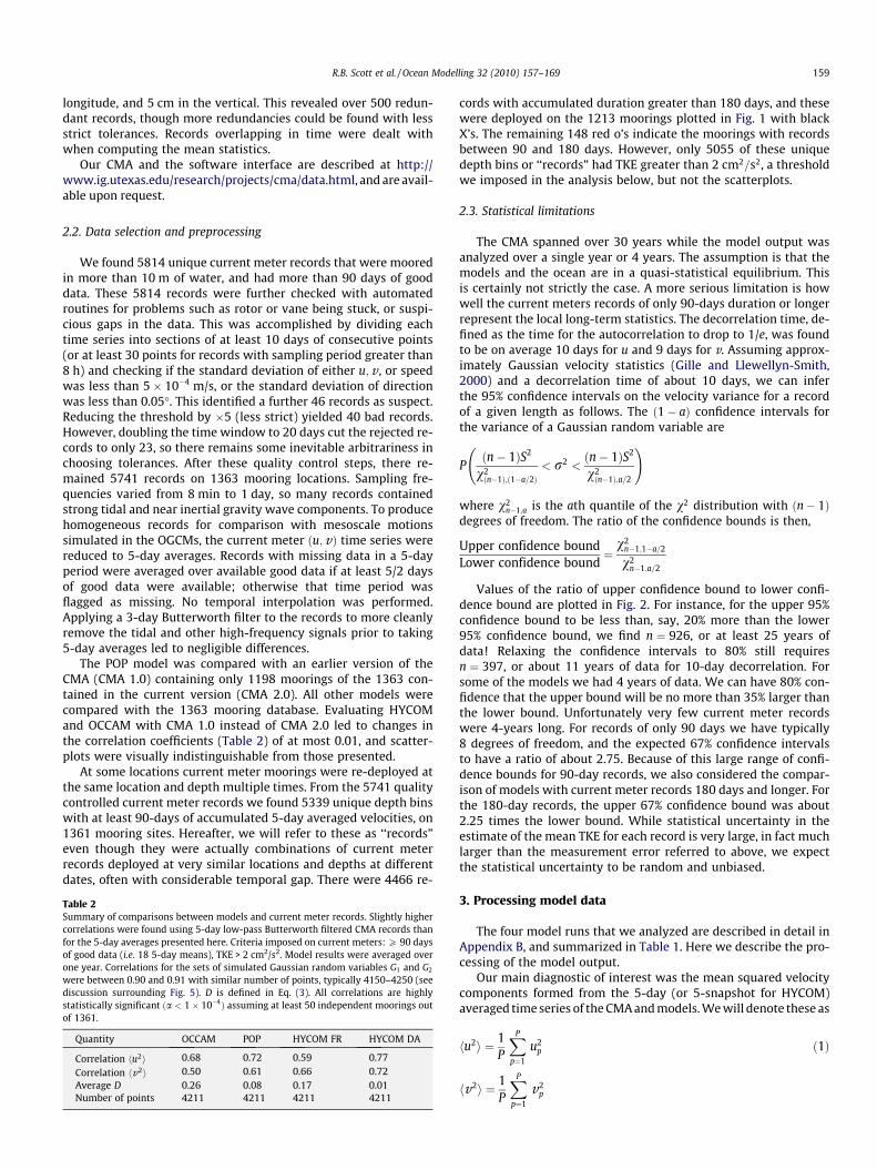
Table 2Summary of comparisons between models and current meter records. Slightly highercorrelations were found using 5-day low-pass Butterworth filtered CMA records thanfor the 5-day averages presented here. Criteria imposed on current meters: P 90 daysof good data (i.e. 18 5-day means), TKE > 2 cm2/s2. Model results were averaged overone year. Correlations for the sets of simulated Gaussian random variables G1 and G2

were between 0.90 and 0.91 with similar number of points, typically 4150–4250 (seediscussion surrounding Fig. 5). D is defined in Eq. (3). All correlations are highlystatistically significant ða < 1� 10�4Þ assuming at least 50 independent moorings outof 1361.

Quantity OCCAM POP HYCOM FR HYCOM DA

Correlation hu2i 0.68 0.72 0.59 0.77

Correlation hv2i 0.50 0.61 0.66 0.72Average D 0.26 0.08 0.17 0.01Number of points 4211 4211 4211 4211

cords with accumulated duration greater than 180 days, and thesewere deployed on the 1213 moorings plotted in Fig. 1 with blackX’s. The remaining 148 red o’s indicate the moorings with recordsbetween 90 and 180 days. However, only 5055 of these uniquedepth bins or ‘‘records” had TKE greater than 2 cm2=s2, a thresholdwe imposed in the analysis below, but not the scatterplots.

2.3. Statistical limitations

The CMA spanned over 30 years while the model output wasanalyzed over a single year or 4 years. The assumption is that themodels and the ocean are in a quasi-statistical equilibrium. Thisis certainly not strictly the case. A more serious limitation is howwell the current meters records of only 90-days duration or longerrepresent the local long-term statistics. The decorrelation time, de-fined as the time for the autocorrelation to drop to 1/e, was foundto be on average 10 days for u and 9 days for v. Assuming approx-imately Gaussian velocity statistics (Gille and Llewellyn-Smith,2000) and a decorrelation time of about 10 days, we can inferthe 95% confidence intervals on the velocity variance for a recordof a given length as follows. The ð1� aÞ confidence intervals forthe variance of a Gaussian random variable are

Pðn� 1ÞS2

v2ðn�1Þ;ð1�a=2Þ

< r2 <ðn� 1ÞS2

v2ðn�1Þ;a=2

!

where v2n�1;a is the ath quantile of the v2 distribution with ðn� 1Þ

degrees of freedom. The ratio of the confidence bounds is then,

Upper confidence boundLower confidence bound

¼v2

n�1;1�a=2

v2n�1;a=2

Values of the ratio of upper confidence bound to lower confi-dence bound are plotted in Fig. 2. For instance, for the upper 95%confidence bound to be less than, say, 20% more than the lower95% confidence bound, we find n ¼ 926, or at least 25 years ofdata! Relaxing the confidence intervals to 80% still requiresn ¼ 397, or about 11 years of data for 10-day decorrelation. Forsome of the models we had 4 years of data. We can have 80% con-fidence that the upper bound will be no more than 35% larger thanthe lower bound. Unfortunately very few current meter recordswere 4-years long. For records of only 90 days we have typically8 degrees of freedom, and the expected 67% confidence intervalsto have a ratio of about 2.75. Because of this large range of confi-dence bounds for 90-day records, we also considered the compar-ison of models with current meter records 180 days and longer. Forthe 180-day records, the upper 67% confidence bound was about2.25 times the lower bound. While statistical uncertainty in theestimate of the mean TKE for each record is very large, in fact muchlarger than the measurement error referred to above, we expectthe statistical uncertainty to be random and unbiased.

3. Processing model data

The four model runs that we analyzed are described in detail inAppendix B, and summarized in Table 1. Here we describe the pro-cessing of the model output.

Our main diagnostic of interest was the mean squared velocitycomponents formed from the 5-day (or 5-snapshot for HYCOM)averaged time series of the CMA and models. We will denote these as

hu2i ¼ 1P

XP

p¼1

u2p ð1Þ

hv2i ¼ 1P

XP

p¼1

v2p

0 50 100 150 200 250 300 350−80

−60

−40

−20

0

20

40

60

80Mooring locations

>180 days

90 to 180 days

Fig. 1. Locations of the 1361 current meter mooring sites used in this study. The 1213 black X’s indicate the moorings with a record at least 180 days long, while the red o’sare the moorings with records between 90 and 180 days. There were a total of 5339 unique depth bins from current meter deployments between September 1973 andFebruary 2005, with at least (accumulated) 90 days of good data. Multiple deployments at the same mooring site and depth are counted as one record or ‘‘unique depth bin”,despite the temporal gap. The sea-floor depth for 76% of moorings was more than 2000 m.

101 102 1031

2

3

4

5

6

7

8

degrees of freedom

Upp

er b

ound

/Low

er b

ound

Range of confidence bounds on variance

95%90%80%67%

Fig. 2. Ratio of the upper confidence bound to lower confidence bound vs. degreesof freedom for various levels of confidence. Current meter records had at least 90days duration, so between 3.5� and 8� of freedom.

160 R.B. Scott et al. / Ocean Modelling 32 (2010) 157–169

where P ¼ 72 for the (default) yearly averages of the model datasince often a few days are missing from the year, and P is the num-ber of pentads available for the individual current meter records(recall minimum P ¼ 18). We will refer to hu2i and hv2i as the meansquared zonal and meridional velocities, and of course 1/2 theirsum is the total kinetic energy (TKE) from the 5-day means.

It is worth mentioning that we did not remove the time meanfrom the velocity time series in Eq. (1). We focused upon TKE sinceeddy kinetic energy (EKE) has a negative bias for shorter records,while Eq. (1) provides an unbiased estimate of TKE.

Before we could form hu2i and hv2i we had to obtain the modeloutput corresponding to the current meter locations. We comparedresults for two methods: using the closest horizontal grid point,and using a weighted average of all the points within a disk sur-rounding the mooring site. The weighted average was of the form:

upðx; y; zi; tÞ ¼P

iupðxi; yi; zi; tÞ wiPiwi

ð2Þ

where wi ¼ expð�ððx� xiÞ2 þ ðy� yiÞ2Þ=a2Þ; ðx; yÞ are coordinates of

the mooring site, a ¼ 9 km, and ðxi; yi; ziÞ are the model grid pointswithin a disk of radius a

ffiffiffi3p

. Grid points below the sea floor weomitted (i.e. wi set to zero). The choice between the two methodswas not critical since about 88% of points had TKE from the twomethods that agreed to within 25%.

For the POP model, daily averaged currents were linearly inter-polated to the latitude and longitude of the mooring sites, whilethe model was run. Model points below the sea floor had zerovelocity (in keeping with no-slip boundary conditions), which re-duced the interpolated flow speed near topography. As mentionedearlier, the POP model was compared with CMA 1.0 which did notcontain all the moorings of CMA 2.0.

For all models the hu2i and hv2i values were interpolated line-arly between vertical grid points to the current meter depths. Cur-rent meter records below the deepest model grid point wereomitted. For the HYCOM model data were only available to thedeepest Levitus grid point of 5500 m. For OCCAM and POP the ver-tical axes extended to 6366 and 5875 m, respectively.

Fig. 4. As in Fig. 3 but for meridional velocity hv2i.

Table 3As in Table 2, but now for current meter records at least 180 days long, and differentmodel durations.

Quantity OCCAM POP HYCOM FR HYCOM DA

Model duration 1 year 1 year 1 year 1 yearCorrelation hu2i 0.68 0.76 0.58 0.80

Correlation hv2i 0.48 0.67 0.70 0.76Average D 0.27 0.09 0.18 0.01Number of points 3510 3510 3510 3510Model duration 4 years 4 yearsCorrelation hu2i 0.68 0.77

Correlation hv2i 0.52 0.70Average D 0.26 0.10Number of points 3692 3692

R.B. Scott et al. / Ocean Modelling 32 (2010) 157–169 161

4. Results

We start with simple log-log scatterplots of mean squared veloc-ities from Eq. (1) with the CMA values on the x-axis, and model valueson the y-axis. Figs. 3 and 4 show the results for hu2i and hv2i. For per-fect agreement between models and observations all the pointswould fall on the thin 45� line. For all models there was considerablescatter about this line, much larger than the measurement error.Nonetheless there was clearly some skill for each of the models.The Pearson correlation coefficient for hu2i and hv2i between modelsand the CMA are presented in Table 2. The scatterplots of hu2i andhv2i were visually similar but the corresponding correlation coeffi-cients revealed that the zonal component was generally modeledmore realistically than the meridional component of TKE. This wasespecially apparent for the OCCAM model, which had the mostanisotropic grid. Restricting the comparison to CMA records of atleast 180 days of accumulated data led to similar, though generallyslightly higher, correlations, see Table 3. Similarly, using four yearsof model data improved the correlations slightly, see lower part ofTable 3. With at least hundreds (if not thousands) of degrees of free-dom, even relatively small correlations would be highly statisticallysignificant.

The large scatter results from a combination of measurementerrors for the current meter records (see Appendix A), statisticaluncertainty in both the current meter records and model time series,and model errors. We need to estimate how much of the scatter re-sulted from statistical uncertainty. Fig. 2 alerts us to the possibility ofvery long records being necessary to produce narrow confidencebounds on EKE, and TKE is dominated by EKE in most places. ForGaussian velocity statistics one could in principle infer the confi-dence bounds on the ratio of sample variances using the F-distribu-tion, but that approach is complicated here by the large number ofrecords with different degrees of freedom. Instead we approachedthis numerically as follows. Consider the case of a perfect modeland perfect current meter records, hampered only by statisticaluncertainty with degrees of freedom chosen to correspond to the ac-tual records we had to analyze. To simulate this situation we createdtwo sets of Gaussian random pseudo time series for each of the 5339current meter records, one set G1 ¼ fg1;1; g1;2; . . . ; g1;Ng; N ¼ 5339 torepresent perfectly accurate CMA records and the other set

Fig. 3. Scatterplot of hu2i from the CMA, and the four OGCMs. The thin verticaldashed line is the threshold above which the correlations quoted in Table 2 werecomputed.

G2 ¼ fg2;1; g2;2; . . . ; g2;Ng; N ¼ 5339 to represent a correspondingperfect OGCM. The pseudo CMA records and the pseudo OGCM areconsidered to measure and simulate a statistically stationary ocean.The difficulty was in choosing appropriate degrees of freedom foreach pair of the 5339 pseudo records. Using the 10-day mean 1=edecorrelation time we found for the CMA 5-day mean u time series,we chose appropriate durations to give the corresponding degrees offreedom. That is, G2 all had 36 independent Gaussian random vari-ables, and each g1 pseudo record had 1/2 the number of 5-day aver-ages in the corresponding real CMA record. Not all of the CMArecords were independent, since current meters are deployed onmoorings with typically several current meters on a single mooring,which reduces the total number of degrees of freedom, and thereforeincreases the statistical uncertainty. To account for this we tried fourassumptions for the Pearson correlation coefficient for pseudo timeseries uðt; zÞ on the same mooring: r ¼ 0;1=2;1; c, where c was cho-sen randomly from the interval [0,1] for each mooring. For each pairof pseudo records the two normally distributed time series werescaled by the same amplitude,rn, implying identical population var-iance r2

n but not necessarily identical sample variances s1;n and s2;n.The amplitudes rn were chosen from the interval ½0; expðz=HÞ�m=swhere z was the depth of the instrument, H ¼ 900 m was the decayscale chosen so that roughly 4100 points were above the threshold of2� 10�4 m2=s2. The scatterplots of the two sets of sample variancesS1 vs. S2 are shown in Fig. 5. There was little sensitivity to the choiceof r.

Fig. 5. Scatterplot of simulated hS21i vs. hS2

2i, the sample variances of pseudo randompseudo CMA records and corresponding pseudo OGCM time series, see Section 4.Subplots are for different values of r, the correlation between pseudo time series atdifferent levels on the same mooring, (a) r ¼ 0, (b) r ¼ 1=2, (c) r ¼ 1, (d) r 2 ½0;1�,chosen randomly. The scatter here is meant to depict the effect of statisticaluncertainty and is the bench mark of perfect CMA records and perfect OGCMs, towhich Figs. 3 and 4 should be compared. The thin vertical dashed line is thethreshold above which the correlations quoted in Table 2 were computed.

−1 −0.5 0 0.5 10

0.1

0.2

HYCOM DA

−1 −0.5 0 0.5 10

0.1

0.2

HYCOM FR

162 R.B. Scott et al. / Ocean Modelling 32 (2010) 157–169

The point is that the discrepancies between the real CMA andOGCM TKE revealed by the scatter in Figs. 3 and 4 should be com-pared to Fig. 5. The qualitative result is that the scatter is clearlygreater for the real CMA and OGCM TKE. The quantitative resultis that a Pearson correlation coefficient between CMA and OGCMTKE of r � 0:9 is the upper bound we expect for a perfect oceanmodel compared to a perfect set of current meters records of thesame duration as our CMA records. And one should bear in mindthat the CMA measurement error was not negligible, see discussionin Appendix A.

How were the modeling errors distributed? Often we can livewith errors if they are random, so what we are especially con-cerned about is identifying biases. For free-running HYCOM andespecially OCCAM, more of the points were below the line thanabove indicating that the model was most often too weak. Andthere were perhaps more points below the line at weaker levels.These biases were difficult to see in these scatterplots, so we turnto another measure.

The model biases were more clear when we examined the fol-lowing statistic, akin to that used by Scott et al. (2008) to comparezonal and meridional velocity variances:

0.2

POP

0.2

OCCAM

D � TKECMA � TKEMOD

TKECMA þ TKEMODð3Þ

−1 −0.5 0 0.5 10

0.1

−1 −0.5 0 0.5 10

0.1

Fig. 6. Distribution of D for the four OGCMs for different depth ranges: 0–750 m(cyan); 750–2000 m (blue); below 2000 m (black).

where the subscripts CMA and MOD refer to the Current Meter Ar-chive and OGCM values, respectively. This normalization maps thediscrepancy to the interval ½�1;1�. We prefer D to considering justthe numerator of D (the unnormalized discrepancy) because it givesa measure of the magnitude of the discrepancy relative to the localenergy level. We prefer not to normalize the discrepancy by just theCMA TKE because the latter also has some error, and when the CMA

TKE happens to be very small, the result becomes very large. That is,the quantity

TKECMA � TKEMOD

TKECMA

maps the discrepancy to the interval ð�1;1Þ, and can exaggeratethe importance of smaller errors. D is defined for each record inour CMA, so we can consider distributions for each model. Perfectagreement between models and observations would result in D dis-tributed like the Dirac-d function. So the more narrowly the histo-gram of D is distributed about the Dirac-d function, the better themodel agrees with observations. We are especially concerned withthe skewness of the distribution. For if D were distributed symmet-rically about zero, there would be no bias, while a distributionskewed to the right indicates the model was too weak relative toobservations. We found the histograms of D to be a sensitive diag-nostic to reveal the model biases.

Fig. 6 presents the histograms of D for all models, and the mean Dis quoted in Tables 2 and 3. In these plots, we have eliminated pointswith TKECMA < 2� 10�4 m2=s2 because the current meter recordsare unreliable at these weak current speeds, see Appendix A. The dis-tributions have been stratified by depth, with the darker colors indi-cating deeper levels. The upper ocean was clearly much bettersimulated than the abyssal ocean. The HYCOM run with data assim-ilation actually had slightly too strong TKE. In contrast to the upperocean, at depth the models were generally biased toward being tooweak relative to the CMA. Clearly none of the models were free ofany bias, but the POP model and the HYCOM model run with dataassimilation stand out as having a much less obvious bias. The rela-tively large values near D ¼ 1 in POP likely represents the few outlierpoints that are much weaker than observations. The mean D in Table2 suggested a similar conclusion as Fig. 6; the smaller mean D of theHYCOM data assimilative model, and POP, are consistent with lessmodel bias. Comparing Tables 2 and 3, we found very similar meanD, suggesting mean D was not strongly influenced by statisticaluncertainty.

As a complementary way to present the bias in vertical struc-ture of horizontal TKE, we also plotted the average of TKE fromall locations within depth bins, see Fig. 7. The depth bins were cho-sen to give roughly similar numbers of observations within eachbin, see thin line with circles. The circles indicate the centre ofthe depth bin. The resulting vertical structure of the currents

10−3 10−2 10−1−5500

−5000

−4500

−4000

−3500

−3000

−2500

−2000−1500

−1000

−500

0

TKE [m2/s2]

Dep

th b

elow

sea

leve

l, [m

]

TKE averaged over all mooring locations

CMAPOPHYCOM DAHYCOM FROCCAMnumber obs

Fig. 7. TKE averaged over all current meter locations vs. depth for all models. Thinline with circles is the number of observations in each depth bin/105 (so there werejust over 300 observations in the depth bin centred just above 4000 m depth). Therewere only 56 observations in the lowest depth bin.

R.B. Scott et al. / Ocean Modelling 32 (2010) 157–169 163

should not be over interpreted since it represents the mean fromdifferent latitudes and longitudes for different depth bins. In form-ing the average, we first averaged over all records on each mooringthat fell within the same depth bin, and then averaged over moor-ings. The number of observations refers to the number of moorings(not the total number of records). We could then resample thesedifferent mooring averages, which were statistically independent,and form the 95% confidence limits using bootstrapping. All mod-els agreed reasonably well with the CMA observations in the upper300 m, but at greater depths the OCCAM and free-running HYCOMmodels were systematically too weak. Below about 4500 m thenumber of available observations (see thin line with circles)dropped off quickly and the comparison is much less significant.In Fig. 8 we plotted the same information, but with a log scale sothat the upper ocean was more clear. Furthermore, we dividedmodel TKE in each bin by the corresponding value in the CMA.

0 0.5 1 1.5 2−10000

−1000

−100

−10TKE averaged over all mooring locations

Dep

th b

elow

sea

leve

l, lo

g sc

ale

[m]

TKE normalized by CMA TKE

CMAPOPHYCOM DAHYCOM FROCCAMnumber obs

Fig. 8. As in Fig. 7 but now normalized by the CMA TKE, a log vertical axis, and thenumber of observations in each depth bin is in thousands. Using the closest gridpoint time series rather than the averaging method shifted the lines less than about0.05 to the right. The thin dashed lines represent the 95% confidence boundsobtained using bootstrapping.

All four models capture the averaged kinetic energy to within fac-tors of 2 to 3 or better. The OCCAM and free-running HYCOM mod-els were around 1.5 times too weak at 300 m depth, about 2 timestoo weak at 3000 m, and about 3 times too weak at 4000 m. How-ever, the POP model had mean TKE profile that agreed with obser-vations to within statistical uncertainty for all depths below1000 m. HYCOM with data assimilation agreed almost as well asPOP with observations below 1000 m, and perhaps slightly betterthan POP above 1000 m.

5. The role of bottom friction in idealized MOM4 experiments

Of the very different model runs described in Table 1, bottomfriction stands out as a possible candidate to explain their differentTKE(z) profiles. In all models the bottom boundary layer feels amomentum drag of the form

ubCd

dh

ffiffiffiffiffiffiffiffiffiffiffiffiffiffiffiffiffiU2

T þ u2b

q� �

where Cd is the dimensionless quadratic drag parameter, dh is thelowest grid cell vertical thickness, ub is the horizontal velocity inthat lowest layer, and UT is the tidal speed – a uniform parameter.Note that UT ¼ 5cm=s, as used in OCCAM and HYCOM, is unrealis-tically strong over most of the deep ocean. For weak bottom flow,jubj � UT , it is clear that UT acts like a linear bottom drag and isnegligible for strong flow jubj UT . We hypothesize that the modelchoices of the two bottom friction parameters, Cd and UT , may ac-count for much of the difference in vertical profile. That POP hasUT ¼ 0 and small Cd and has the most energy in the deep ocean ofthe three free running models shown in Fig. 8 is suggestive that bot-tom friction may be dampening OCCAM and HYCOM FR excessively.Unfortunately confirming this hypothesis rigorously via multipleexperiments with extremely expensive global OGCMs was not prac-tical. Instead, here we explore the sensitivity of TKE(z) profile tobottom friction in a controlled set of experiments with the ModularOcean Model (MOM4, http://www.gfdl.noaa.gov/ocean-model).

MOM4 was setup in an idealized midlatitude, kidney beanshaped, basin from 20 to 40 �N and of 10� longitudinal width, withcontinental slopes, some sea-floor roughness, a seamount and anelongated ridge. Circulation was spun-up from rest, with an expo-nential initial potential temperature profile, for 50 years. The forcingconsisted of constant zonal, cosine in latitude, double-gyre windstress of peak amplitude 0.1 Pa, and SST relaxation to prescribedSST decreasing linearly with latitude. The resolution was 1/12� lati-tude and longitude and 40 vertical levels. The model was simply con-figured: linear equation of state based upon temperature alone witha ¼ 0:0015, no Gent-McWilliams (GM) parameterization, constantbiharmonic ð6:3� 109 m4=sÞ, laplacian ð10:7 m2=sÞ, and vertical vis-cosity ð1� 10�4 m2=sÞ. Each model run was spun-up for 15 years toreach equilibrium with different bottom friction parameters.

Fig. 9 shows the results of three MOM4 simulations that areidentical except for changing the bottom friction parameters Cd

and UT . The first run (green) is POP-like in its bottom frictionparameters, see Table 1. Increasing bottom friction by increasingUT to 5 cm=s, as in OCCAM, reduced the upper ocean TKE ratherdramatically (red line in subplot a), but actually increased the lowerocean TKE. This counter intuitive effect requires considering thecoupling between different modes. We have decomposed the TKEinto barotropic, (BT), baroclinic, (BC), and cross-term contributions,(BX), so that

TKEðzÞ ¼ 12hu ui ¼ 1

2hu2

btiBT

þ12hu2

bciBC

þhubt ubciBX

ð4Þ

where u is the 5-day average velocity, and hi denotes average overfour years and over the part of the basin with sea-floor depth great-

0 0.01 0.02−1000

−500

0(a)

−2 0 2

x 10−3

−3000

−2000

−1000(b)

−6 −4 −2 0x 10

−3

−1000

−500

0(c)

−2 0 2 4 6

x 10−4

−3000

−2000

−1000(d)

Fig. 9. TKE vs depth for three MOM4 simulations, exploring the effects of Cd and UT . The upper row, subplots (a) and (c), are for the upper 1000 m while the lower row is forthe deeper ocean. The left column, subplots (a) and (b), show the TKE profile averaged over the basin where it was deeper than 2000 m. The TKE is decomposed into thebarotropic (thin straight), baroclinic (thin curvy line), cross-term (dashed), and total (thick solid line). The colors correspond to three runs: Cd ¼ 0:001 and UT ¼ 0 cm=s(green), Cd ¼ 0:001 and UT ¼ 5 cm=s (red), Cd ¼ 0:0022 and UT ¼ 5 cm=s (blue). The right column, subplots (b) and (d) shows the difference between from the green line in(a) and (d), respectively.

0.7 0.8 0.9 1 1.1 1.2 1.3 1.4−3500

−3000

−2500

−2000

−1500

−1000

−500

0Effect of Cd and UT

TKE over TKE from reference case

dept

h [m

]

reference caseUT =5cm/s

UT =5cm/s & Cd=0.0022

Fig. 10. TKE(z) divided by TKE(z) for the reference case ðCd ¼ 0:001 and UT ¼ 0Þ vs.depth for the two perturbation MOM4 simulations shown in Fig. 9.

164 R.B. Scott et al. / Ocean Modelling 32 (2010) 157–169

er than 2000 m. The BT mode was found via a depth average of the5-day average velocity, and the BC component was the residual.Note the cross-term is positive where the BT and BC flow are posi-tively correlated and negative where they are anticorrelated. Thecross-term contributes to the vertical profile but integrates overdepth to zero by construction.

The BT and BC modes had reduced TKE (blue thin straight andcurvy lines are to the left of green lines in b), as one might expectfrom increasing bottom friction by increasing UT from UT ¼ 0 cm=sto UT ¼ 5 cm=s. But the modes became less strongly coupled. In thedeeper ocean where BT and BC are anticorrelated the weaker cou-pling increased the TKE – the dashed blue in (b) is less negative,while in the upper ocean where BT and BC were positively corre-lated the weaker coupling decreased the TKE. These changes aremore clearly resolved in the right subplots (c) and (d), showingthe difference from the green lines in (a) and (b), respectively.For instance in (d) we see clearly that the reduction in BT and BCTKE was overwhelmed by the much stronger increase in thecross-term ‘‘BX”. Arbic and Flierl (2004) explain how linear bottomfriction acting alone in the 2-layer QG model can increase couplingbetween the BT and BC modes. But here we observed that UT actsto decouple the barotropic and baroclinic modes.

Further increasing the bottom friction by increasing Cd by 220%to Cd ¼ 0:0022 (as in HYCOM, blue lines) had more straightforwardeffects. The upper ocean flow was almost unchanged (blue and redlines very similar in Fig. 9a). And indeed the BT, BC, and BX contri-butions in the upper ocean were also hardly affected. The deepocean TKE was weakened by the stronger quadratic drag withCd ¼ 0:0022, and the strongest contributor was the increased BXterm. The smaller horizontal scale of subplot (b) for the deeperocean shows that, not surprisingly, the BT flow was somewhatweaker due to the stronger quadratic drag, but the BC energiesfor Cd ¼ 0:0022 and Cd ¼ 0:001 were very similar (thin blue andred lines). Stronger quadratic drag enhanced BT and BC coupling,much like linear drag does (Arbic and Flierl, 2004). In fact in QGsimulations, linear and quadratic bottom drag have similar effectson eddies (Arbic and Scott, 2008).

The above experiments revealed that UT affects mostly the cou-pling between BT and BC modes, and therefore has an antisymmet-ric response in the upper and lower ocean. In contrast the Cd

parameter primarily dampens both the BT and BC flow, reducingthe depth-integrated TKE and TKE(z) in both the upper and lowerocean, with the reduction in the deeper ocean being partly offsetby strengthening the coupling between BT and BC. The Cd param-eter is critical and its 220% increase reduced the TKE(z) by up to30% in the deep ocean and slightly more in the upper ocean, seeFig. 10.

For most depths in Fig. 8, HYCOM TKE was within 30% of obser-vations when error bars are taken into account. These idealizedMOM4 experiments suggest that reducing Cd in HYCOM from0.0022 to 0.001 could potentially bring its profile of TKE(z) to with-

0.2

HYCOM DA

0.2

HYCOM FR

R.B. Scott et al. / Ocean Modelling 32 (2010) 157–169 165

in error bars of observations. Reducing the UT parameter to speedsmore typical of the deep ocean could further improve the fit. It isless clear that OCCAM would have more realistic TKE(z) with fur-ther tuning of the bottom friction parameters.

−1 −0.5 0 0.5 10

0.1

−1 −0.5 0 0.5 10

0.1

−1 −0.5 0 0.5 10

0.1

0.2

POP

−1 −0.5 0 0.5 10

0.1

0.2

OCCAM

Fig. 11. As in Fig. 6 but the results are stratified by latitude (as opposed to depth):0–20� (cyan); 20–45� (blue); >45� (black).

6. Summary and discussion

A large collection of moored current meter records from a re-cently assembled current meter archive (CMA) was used to assessthe ability of four eddying OGCMs to simulate the time-averagedtotal kinetic energy (TKE) throughout the water column. The mainresult was that the vertical profile of TKE(z) averaged over allmooring sites agreed with the TKE(z) profile from all model runs(sampled at the mooring sites) to within a factor of two above3500 m depth, and a factor of 3 at all depths. Some caveats on theseresults are as follows.

Moored current meters have inherent limitations, as discussedin Section 2 and Appendix A. Measurement errors can be as largeas 45% for TKE for acoustic current meters under challenging con-ditions of low current speeds and low suspended particle densityat depth. However, generally measurement errors were muchsmaller. Mooring blow-over was also a concern, since about 10%of the records had 25% of their measurements from depths morethan 70 m below their nominal deployment depth. This results instrong currents being underestimated by subsurface mooring cur-rent meters.

There was found to be considerable scatter in the comparisonbetween TKE in the eddying OGCMs and the CMA, even larger thanthe statistical uncertainty, implying that models cannot be trustedto give reliable TKE at arbitrary locations. This is similar to the find-ings of Arbic et al. (2009), who compared models and an earlierversion of our CMA at the bottom (rather than throughout thewater column, as done here), and of Penduff et al. (2006), wholooked at the Atlantic CLIPPER model and WOCE current meters.However, there was highly significant correlation between thesimulated and observed TKE, suggesting some model skill. Wewere mostly concerned with identifying any model bias in the ver-tical distribution of TKE. Scatterplots were only slightly useful forrevealing model biases. A much more sensitive diagnostic wasthe distribution of discrepancy between simulated and observedTKE, scaled by their sum, see Eq. (3). All models had some bias,and the bias tended to be toward too weak simulated currents atgreater depths. However, the HYCOM model with data assimila-tion, and the (free running) POP model had much less obvious bias.An average taken over all current meters, plotted vs. binneddepths, also showed that these two simulations yielded the leastbias over the full-water column.

Penduff et al. (2006) suggest that horizontal resolution may bethe most important factor limiting the CLIPPER OGCM in generat-ing realistic EKE, since the first Rossby radius of deformation wasbest resolved at low-latitudes, and the model-data comparisonwas most favorable there. A preliminary analysis herein suggeststhe situation is complicated. Fig. 11 shows the distribution of Dfor low, mid and high latitudes. While Penduff et al.’s suggestionappears to be consistent with the results for the HYCOM modelwith data assimilation, one must keep in mind that no data assim-ilation were performed north of 47 �N. The POP model was actuallybimodal, revealing both strong and weak biases at high latitudes.This issue clearly deserves more attention.

Deciphering why one model performs better than another is dif-ficult because controlled experiments are currently not feasible forglobal eddying OGCMs. As an alternative, we performed multiplecontrolled experiments varying the bottom friction in MOM4 runfor a regional idealized basin. Increasing the UT parameter wasfound to decrease the coupling between barotropic (BT) and baro-

clinic (BC) flow, and therefore to increase the basin mean TKE(z)below 1000 m while decreasing TKE(z) above 1000 m. The upshotfor interpreting the global eddying models studied herein was thatthe unrealistically strong UT ¼ 5cm=s of OCCAM and HYCOM wasnot likely to be the source of their too sheared TKE(z) relative toobservations. Reducing Cd should reduce the amplitude of boththe BT and BC modes. It is difficult to extrapolate quantitativelyto the HYCOM model, but for our idealized MOM4 simulationdecreasing Cd from Cd ¼ 0:0022 to Cd ¼ 0:001 accounted for a30% increase in TKE below 1000 m. A similar improvement in HY-COM would bring it to within error bars of the observed TKE(z).The apparent sensitivity of the models examined here to bottomdrag shares some similarities to the drag sensitivities investigatedin earlier studies using both idealized (e.g. Arbic and Flierl, 2004;Riviere et al., 2004; Thompson and Young, 2006; Arbic and Scott,2008) and realistic (Hurlburt and Hogan, 2008) models.

Quadratic bottom drag is certainly not the only parameterresponsible for the model differences. The sensitivity of model re-sults to the model formulation and associated numerical treatmentis not fully documented (Griffies et al., 2000, 2009) and several stud-ies show that the modeled circulation remains quite sensitive to thechoices made for subgrid scale parameterizations (Chassignet andMarshall, 2008; Hecht and Smith, 2008; Hecht et al., 2008). Whilebathymetry is an important consideration in general, the differencesin its numerical treatment between the three models appear minor;like POP, OCCAM also used partial bottom cells with a z-grid as well(though OCCAM was also hindered by decreasing horizontal resolu-tion at higher latitudes by an anisotropic grid), and the generalizedvertical coordinate of HYCOM, while different in approach, leads tocomparable flexibility. Important differences in the forcing werethe monthly forcing of POP, which did not include the higher fre-quency forcing that tends to excite high frequency vertical motionsthat increase numerical diffusion. Dramatic examples of the depen-dence of vertical velocity on forcing frequency are shown by Klein(2008, Plates 4 and 5).

Acknowledgements

We benefitted from conversations with Carl Wunsch. Twoanonymous reviews helped improve the manuscript. We are grate-ful to Carl Wunsch for contributing generously to our CMA, and tothe Buoy Group at Oregon State University for maintaining theirDeep Water Archive (OSU DWA).

200

400

600

800

1000

1200

1400Maximum blow−over

num

ber o

f CM

reco

rds

200

400

600

800

1000

1200

1400Interquartile range

num

ber o

f CM

reco

rds

166 R.B. Scott et al. / Ocean Modelling 32 (2010) 157–169

R.B.S. thanks the National Oceanography Centre, Southampton(NOCS) for hosting an extended visit. The authors acknowledgethe Texas Advanced Computing Center (TACC) at The Universityof Texas at Austin for providing High-Performance Computing(HPC) resources that have contributed to the research results re-ported within this paper, http://www.tacc.utexas.edu. R.B.S. wassupported by National Science Foundation (NSF) grants OCE-0526412 and OCE-0851457, a grant from King Abdullah Universityof Science and Technology (KAUST), and NOCS. B.K.A. and A.V. weresupported by NSF grant OCE-0623159 and a Jackson School of Geo-sciences Development Grant. M.M. was supported by the DOE Of-fice of Science Climate Change Prediction Program. This is UTIGcontribution #2182.

This paper is dedicated to the memory of the great physicaloceanographer and journal editor Peter Killworth.

0 1000 20000

pressure in db0 200 400

0

pressure in db

Fig. 12. Distribution of statistics for 1559 current meters with co-located pressuresensors. Left: Histogram of the interquartile range of pressure from each pressurerecord. Right: Histogram of the minimum to maximum range of pressure (revealingmaximum vertical displacement occurring in each pressure record).

Appendix A. General limitations of moored current meterrecords

The reader should bear in mind the inherent limitations of Eule-rian current statistics from moored current meters. These are re-viewed briefly.

Subsurface moorings in deep water rarely have measurementswithin the upper 200 m. Their most serious limitation is that theytend to blow over in strong currents, effectively providing a mea-surement at varying depths that are, when currents are stronger,lower in the water column than their nominal depth. The problemcan be tracked for moorings with pressure sensors, and can bequite substantial, with hydrostatic pressure variations reaching1000 db or more. Schemes have been devised to correct for blow-over of moorings without pressure sensors (Hogg, 1991; Meinenand Luther, 2002). To the best of our knowledge, none of the re-cords in our archive were corrected for mooring blow-over(Wunsch, pers. comm. 2009; Joseph Bottero, pers. comm. 2009),and we did not attempt any corrections.

Fig. 12 shows the distribution of blow-over from all the recordsin our database that had reliable pressure recordings at the samedepth as the current meters. From the distribution of interquartilerange of pressure we see that most current meters spent at leasthalf their deployment within a few dozen db of their mediandepth, but the most extreme case had half its measurements170 db above or below its median depth. About 10% of the recordshad 25% of their measurements from depths more than 70 db be-low their minimum depth. For the model comparison in Section4 we used the nominal depth given for each record, since not all re-cords had pressure sensors to estimate the mean depth. Maximumblow-over greater than a few hundred db was rare, but the worstcase reached 1860 db. Blow-over introduces a bias in our estimatesof TKE because these strong events tend to be underestimated. Oneshould also note that observationalists tend to avoid deployingmoorings in the very strongest currents so as to avoid strongblow-over, which introduces some bias in the sampling of theocean we have for comparison. On the other hand, moorings are of-ten deployed in oceanographically interesting places, which wefound includes some bias toward sampling stronger current re-gions (e.g. Sen et al., 2008).

Surface moorings can provide measurements near the surfacewithout the problems of blow-over, but have other problems. Dur-ing the MODE experiment (MODE Group, 1978) it was discoveredthat surface moorings can give faulty measurements (exaggeratingTKE by a factor of five or more for measurements below 500 m) dueto a mode of oscillation excited by surface waves (Gould et al.,1974). The dual propeller Vector Measuring Current Meters(VMCM) (Weller and Davis, 1980) are generally used on surfacemoorings since field tests showed them to be less affected by wave

motion (Halpern et al., 1981). Compliant elements of the mooringare also now used to tune the resonance outside the strong signalsin the surface wave band. Of course current meters can only be ex-pected to measure water velocities relative to the moving surfacebuoy. Plueddemann and Farrar (2006) estimate the errors thisintroduces to absolute near-inertial current measurements. Forthe TKE of interest here, the error estimates would be difficult,and not clearly of one sign. (The surface buoys must have someslack to minimize static tension in strong winds. To quote an ex-treme example, Plueddemann et al. (1995) found a mooring length1.25 times the water depth to be necessary to survive the challeng-ing environment of the subarctic North Atlantic; this allowed thesurface mooring to drift in a circle of radius 3/4 of the water depth.)

The CMA described in Section 2 includes measurements from avariety of sensors from different manufacturers. Mechanicaldevices include the vector averaging current meter (VACM) devel-oped in the 1960s at Woods Hole Oceanographic Institution andvector measuring current meter (VMCM) (Weller and Davis,1980). An important limitation of these mechanical current metersis their minimum detectable current speed, below which the rotorstalls. This varies with sensor, with typical stall speeds of 1–2 cm/s.Recorded speeds less than the stall speed are handled differentlyby different investigators. For instance, speeds less than the stallspeed might be set to 1/2 the stall speed, in a crude attempt tominimize the error in mean statistics. Acoustic current meters onthe other hand rely on either the Doppler shift of echos from sus-pended particles (Acoustic Doppler Current Profilers or ADCP) orthe difference in acoustic travel time between sensor pairs(VCM). Hogg and Frye (2007) compared two VACMs with twoacoustic current meters, an Aanderaa RCM11 ADCP and a NobskaMAVS VCM all near 2000 m in a deep-water mooring south eastof Bermuda. The ADCP measured speeds about 10–25% lower (i.e.TKE up to 45% lower) than the reference VACMs for current speedsup to about 15 cm/s. The VCM had a constant offset from theVACMs of about 2–3 cm/s. The investigators emphasized the chal-lenging conditions of the comparison: low current speeds and clearwater (low scattering levels).This is a reasonable interpretationsince Gilboy et al. (2000) found an agreement to within statisticaluncertainty between a VACM, a VCM and an ADCP at a nearby siteand at 72 m instrument depth (where the ocean is more energeticand contains more suspended particles for scattering).

R.B. Scott et al. / Ocean Modelling 32 (2010) 157–169 167

Appendix B. Models

Description of POP model runs

POP (Parallel Ocean Program, http://climate.lanl.gov/Models/POP/) is a publicly available, z-level, hydrostatic, Boussinesq, prim-itive equation ocean model that allows for generalized orthogonalhorizontal grids. It is an implicit free surface derivative of the ori-ginal Bryan-Cox model with improved numerics that have beenwidely tested. It has a wide user base and was the ocean compo-nent of the NCAP CCSM3.0 climate model that contributed to theIntergovernmental Panel on Climate Change Fourth AssessmentReport. It is being used in very high resolution coupled climatesimulations as part of the LLNL grand challenge project.

We analyzed an updated version of the 1/10� grid POP modeldescribed by Maltrud and McClean (2005) that has several signifi-cant changes. The horizontal grid was modified in the NorthernHemisphere, moving from a dipole to a tripole version, resultingin more uniform resolution in the Arctic. There are 42 vertical lev-els, ranging from 10 m at the surface to 250 m at depth. Full-cellbottom topography (generated from ETOPO2; ETOPO2, 2006) wasreplaced with partial bottom cells (Adcroft et al., 1997). Verticaldiffusion coefficients were calculated using KPP (Large et al.,1994), and biharmonic representations of subgrid momentumand tracer diffusion were used, but with lower values than inMaltrud and McClean (2005). Surface forcing was calculated fromthe ‘‘normal year” of the CORE dataset (Large and Yeager, 2004),averaged in time from 6-hourly to monthly. The POP model runwas described further by Maltrud et al. (2008, 2009).

We converted the daily averages from years 48 to 52 to 5-dayaverages for comparison with the CMA. See further discussion inSection 3 below.

10 20 30 40 50 60 70−0.5

0

0.5

m/s

Emperor Seamounts: zonal full and geostrophic velocity

10 20 30 40 50 60 70−0.2

0

0.2

m/s

10 20 30 40 50 60 70−0.1

0

0.1

m/s

10 20 30 40 50 60 70−0.05

0

0.05

m/s

5−day intervals

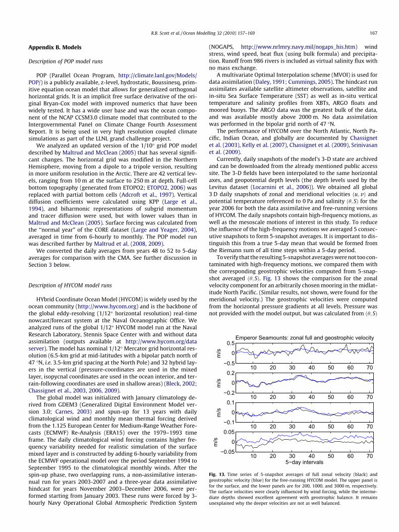
Fig. 13. Time series of 5-snapshot averages of full zonal velocity (black) andgeostrophic velocity (blue) for the free-running HYCOM model. The upper panel isfor the surface, and the lower panels are for 200, 1000, and 3000 m, respectively.The surface velocities were clearly influenced by wind forcing, while the interme-diate depths showed excellent agreement with geostrophic balance. It remainsunexplained why the deeper velocities are not as well balanced.

Description of HYCOM model runs

HYbrid Coordinate Ocean Model (HYCOM) is widely used by theocean community (http://www.hycom.org) and is the backbone ofthe global eddy-resolving (1/12� horizontal resolution) real-timenowcast/forecast system at the Naval Oceanographic Office. Weanalyzed runs of the global 1/12� HYCOM model run at the NavalResearch Laboratory, Stennis Space Center with and without dataassimilation (outputs available at http://www.hycom.org/dataserver). The model has nominal 1/12� Mercator grid horizontal res-olution (6.5-km grid at mid-latitudes with a bipolar patch north of47 �N, i.e. 3.5-km grid spacing at the North Pole) and 32 hybrid lay-ers in the vertical (pressure-coordinates are used in the mixedlayer, isopycnal coordinates are used in the ocean interior, and ter-rain-following coordinates are used in shallow areas) (Bleck, 2002;Chassignet et al., 2003, 2006, 2009).

The global model was initialized with January climatology de-rived from GDEM3 (Generalized Digital Environment Model ver-sion 3.0; Carnes, 2003) and spun-up for 13 years with dailyclimatological wind and monthly mean thermal forcing derivedfrom the 1.125 European Center for Medium-Range Weather Fore-casts (ECMWF) Re-Analysis (ERA15) over the 1979–1993 timeframe. The daily climatological wind forcing contains higher fre-quency variability needed for realistic simulation of the surfacemixed layer and is constructed by adding 6-hourly variability fromthe ECMWF operational model over the period September 1994 toSeptember 1995 to the climatological monthly winds. After thespin-up phase, two overlapping runs, a non-assimilative interan-nual run for years 2003-2007 and a three-year data assimilativehindcast for years November 2003–December 2006, were per-formed starting from January 2003. These runs were forced by 3-hourly Navy Operational Global Atmospheric Prediction System

(NOGAPS, http://www.nrlmry.navy.mil/nogaps_his.htm) windstress, wind speed, heat flux (using bulk formula) and precipita-tion. Runoff from 986 rivers is included as virtual salinity flux withno mass exchange.

A multivariate Optimal Interpolation scheme (MVOI) is used fordata assimilation (Daley, 1991; Cummings, 2005). The hindcast runassimilates available satellite altimeter observations, satellite andin-situ Sea Surface Temperature (SST) as well as in-situ verticaltemperature and salinity profiles from XBTs, ARGO floats andmoored buoys. The ARGO data was the greatest bulk of the data,and was available mostly above 2000 m. No data assimilationwas performed in the bipolar grid north of 47 �N.

The performance of HYCOM over the North Atlantic, North Pa-cific, Indian Ocean, and globally are documented by Chassignetet al. (2003), Kelly et al. (2007), Chassignet et al. (2009), Srinivasanet al. (2009).

Currently, daily snapshots of the model’s 3-D state are archivedand can be downloaded from the already mentioned public accesssite. The 3-D fields have been interpolated to the same horizontalaxes, and geopotential depth levels (the depth levels used by theLevitus dataset (Locarnini et al., 2006)). We obtained all global3 D daily snapshots of zonal and meridional velocities ðu;vÞ andpotential temperature referenced to 0 Pa and salinity ðh; SÞ for theyear 2006 for both the data assimilative and free-running versionsof HYCOM. The daily snapshots contain high-frequency motions, aswell as the mesoscale motions of interest in this study. To reducethe influence of the high-frequency motions we averaged 5 consec-utive snapshots to form 5-snapshot averages. It is important to dis-tinguish this from a true 5-day mean that would be formed fromthe Riemann sum of all time steps within a 5-day period.

To verify that the resulting 5-snapshot averages were not too con-taminated with high-frequency motions, we compared them withthe corresponding geostrophic velocities computed from 5-snap-shot averaged ðh; SÞ. Fig. 13 shows the comparison for the zonalvelocity component for an arbitrarily chosen mooring in the midlat-itude North Pacific. (Similar results, not shown, were found for themeridional velocity.) The geostrophic velocities were computedfrom the horizontal pressure gradients at all levels. Pressure wasnot provided with the model output, but was calculated from ðh; SÞ

168 R.B. Scott et al. / Ocean Modelling 32 (2010) 157–169

by simply converting h to in situ temperature, and in situ densityusing MatLab Seawater routines (http://www.cmar.csiro.au/data-centre/ext_docs/seawater.htm), which contain the fully nonlinearequation of state. We vertically integrated the density using the sim-ple trapezoidal rule. The horizontal gradients were computed using aweighted least squares fit of a 2 D plane to all the points within a diskof radius 9 km. (The weights are described below, see Eq. (2)). The sealevel gradient was used to obtain the surface geostrophic flow. At thesurface, see upper panels, the full 5-snapshot average velocity (blacklines) clearly had more variability than the geostrophic velocity(blue lines), presumably due to the direct wind forcing in the Ekmanlayer. At 200 and 1000 m depth (two middle panels) the comparisonwas good enough to suggest that 5-snapshot averages were not con-taminated with high-frequency motions. At 3000 m the velocity wasquite weak, and the comparison was not as good. We are unsure whythe deep velocities appear less geostrophic, though smoothing of thedensity field resulting from mapping from the hybrid coordinates tothe regular grid at Levitus depth levels may be responsible.

OCCAM model run

The global 1/12� Ocean Circulation and Climate Advanced Mod-elling Project (OCCAM) is, like the POP model, based upon the z-le-vel coordinate representation of the Boussinesq primitiveequations, first used in GFDL’s MOM model. The model horizontalresolution for OCCAM is non-isotropic, employing a regular 1/12�latitude-longitude grid outside the Arctic and North Atlantic. Inthe North Atlantic and Arctic, the grid has been rotated to avoidthe polar singularity, as explained at www.noc.soton.ac.uk/JRD/OCCAM/EMODES/info/coord.php3. MatLab routines to do the rota-tion are provided at www.ig.utexas.edu/people/staff/rscott/personal.htm. The vertical resolution was 66 levels with spacing rang-ing from 5 m near the surface to 200 m in the deep ocean. Topog-raphy was based upon Smith and Sandwell (1997), and therepresentation included partial bottom cells. Vertical viscositywas 1� 10�4 m2=s and the horizontal viscosity was 50 m2=s. OC-CAM was forced with high frequency atmospheric fields from theNational Centers for Environmental Prediction (NCEP) reanalysis.Evaporation, together with latent, sensible, and long-wave heatfluxes, were calculated at each time step from bulk formulae, usinginterpolated 6-hourly atmospheric fields and model sea surfacetemperature. Insolation was provided by monthly average valuesapplied with a simulated diurnal cycle. The forcing fields and othermodel details are described further by Lee et al. (2007).

The model is integrated from rest with initial tracer fields fromthe annual mean World Ocean Circulation Experiment Special Anal-ysis Center climatological values (Gouretski and Jancke, 1996). Themodel has been run starting with model year 1985, and we analyzed5-day means from 1999 to 2003 and, separately, from 2004.

References

Adcroft, A., Hill, C., Marshall, J., 1997. Representation of topography by shaved cellsin a height coordinate ocean model. Mon. Weather Rev. 125, 2293–2315.

Arbic, B.K., Flierl, G.R., 2004. Baroclinically unstable geostrophic turbulence in thelimits of strong and weak bottom Ekman friction: application to midoceaneddies. J. Phys. Oceanogr. 34, 2257–2273.

Arbic, B.K., Scott, R.B., 2008. On quadratic bottom drag, geostrophic turbulence, andoceanic mesoscale eddies. J. Phys. Oceanogr. 38, 84–103.

Arbic, B.K., Shriver, J.F., Hogan, P.J., Hurlburt, H.E., McClean, J.L., Metzger, E.J., Scott,R.B., Sen, A., Smedstad, O.M., Wallcraft, A.J., 2009. Estimates of bottom flows andbottom boundary layer dissipation of the oceanic general circulation fromglobal high-resolution models. J. Geophys. Res. 114, C02024.

Barnier, B., Madec, G., Penduff, T., Molines, J.-M., Treguier, A.-M., Le Sommer, J.,Beckmann, A., Biastoch, A., Böning, C., Dengg, J., Derval, C., Durand, E., Gulev, S.,Remy, E., Talandier, C., Theetten, S., Maltrud, M., McClean, J., De Cuevas, B., 2006.Impact of partial steps and momentum advection schemes in a global oceancirculation model at eddy-permitting resolution. Ocean Dynam. 56, 543–567.

Bleck, R., 2002. An oceanic general circulation model framed in hybrid isopycniccartesian coordinates. Ocean Modell. 4, 55–88.

Carnes, M.R., 2003. Description and evaluation of GDEM-v 3.0. Naval OceanographicOffice Technical Note.

Chassignet, E., Hurlburt, H., Smedstad, O., Halliwell, G., Hogan, P., Wallcraft, A.,Bleck, R., 2006. Ocean prediction with the hybrid coordinate ocean model(HYCOM). In: Chassignet, E., Verron, J. (Eds.), Ocean Weather Forecasting.Springer, pp. 413–426.

Chassignet, E.P., Hurlburt, H.E., Metzger, E.J., Smedstad, O.M., Cummings, J.A.,Halliwell, G.R., Bleck, R., Baraille, R., Wallcraft, A.J., Lozano, C., Tolman, H.L.,Srinivasan, A., Hankin, S., Cornillon, P., Weisberg, R., Barth, A., He, R., Werner, F.,Wilkin, J., 2009. US GODAE Global Ocean Prediction with the HYbrid CoordinateOcean Model (HYCOM). Oceanography 22 (2, Sp. Iss. SI), 64–75.

Chassignet, E.P., Marshall, D.P., 2008. Gulf stream separation in numerical oceanmodels. In: Hecht, Hasumi (Eds.), Ocean Modeling in an Eddying Regime. AGUMonograph Series. AGU, pp. 39–62.

Chassignet, E.P., Smith, L.T., Halliwell, G.R., Bleck, R., 2003. North Atlanticsimulations with the HYbrid Coordinate Ocean Model (HYCOM): impact ofthe vertical coordinate choice, reference pressure, and thermobaricity. J. Phys.Oceanogr. 33, 2504–2526.

Colin de Verdiere, A., Mercier, H., Arhan, M., 1989. Mesoscale variability fromthe western to the eastern Atlantic along 48 �N. J. Phys. Oceanogr. 19,1149–1170.

Cummings, J.A., 2005. Operational multivariate ocean data assimilation. Quart. J. R.Met. Soc. 131, 3583–3604.

Daley, R., 1991. Atmospheric Data Analysis. Cambridge Atmospheric and SpaceScience Series. Cambridge University Press.

ETOPO2, 2006. 2-Minute gridded global relief data (ETOPO2v2). U.S. Department ofCommerce, National Oceanic and Atmospheric Administration, NationalGeophysical Data Center.

Gilboy, T., Dickey, T., Sigurdson, D., Yu, X., Manov, D., 2000. An intercomparison ofcurrent measurements using a vector measuring current meter, an acousticDoppler current profiler, and a recently developed acoustic current meter. J.Atmos. Oceanic Technol. 17 (4), 561–574.

Gille, S.T., Llewellyn-Smith, S.G., 2000. Velocity probability density functions fromaltimetry. J. Phys. Oceanogr. 30, 125–136.

Gould, W.J., Schmitz, W.M., Wunsch, C., 1974. Preliminary field results for a midocean dynamics experiment (MODE-O). Deep-Sea Res. 21, 911–932.

Gouretski, V.V., Jancke, K., 1996. A new hydrographic data set for the South Pacific:synthesis of WOCE and historical data. WHP SAC Tech. Rep. 2, WOCE Rep. 143/96, 110 pp.

Griffies, S.M., Biastoch, A., Böning, C., Bryan, F., Danabasoglu, G., Chassignet, E.,England, M., Gerdes, R., Haak, H., Hallberg, R., Hazeleger, W., Jungclaus, J., Large,W., Madec, G., Pirani, A., Samuels, B., Scheinert, M., Gupta, A., Severijns, C.,Simmons, H., Treguier, A.-M., Winton, M., Yeager, S., Yin, J., 2009. Coordinatedocean-ice reference experiments (COREs). Ocean Modell. 26, 1–46.

Griffies, S.M., Böning, C., Bryan, F., Chassignet, E., Gerdes, R., Hasumi, H., Hirst, A.,Treguier, A.-M., Webb, D., 2000. Developments in ocean climate modelling.Ocean Modell. 2, 123–192.

Halpern, D., Weller, R.A., Briscoe, M.G., Davis, R.E., McCullough, J.R., 1981.Intercomparison tests of moored current measurements in the upper ocean. J.Geophys. Res. 86 (NC1), 419–428.

Hecht, M.W., Hasumi, H. (Eds.), 2008. Ocean Modeling in an Eddying Regime. AGUMonograph Series. AGU.

Hecht, M.W., Hunke, E., Maltrud, M.E., Petersen, M.R., Wingate, B.A., 2008. Lateralmixing in the eddying regime and a new broad-ranging formulation. In: Hecht,Hasumi (Eds.), Ocean Modeling in an Eddying Regime. AGU Monograph Series.AGU, pp. 339–352.

Hecht, M.W., Smith, R.D., 2008. Towards a physical understanding of the NorthAtlantic: a review of model studies in an eddying regime. In: Hecht, Hasumi(Eds.), Ocean Modeling in an Eddying Regime. AGU Monograph Series. AGU, pp.213–240. Available from: %3chttp://public.lanl.gov/mhecht/preprints/NA_pp.pdf%3e.

Hogg, N.G., 1991. Mooring motion corrections revisited. J. Atmos. Oceanic Technol.8, 289–295.

Hogg, N.G., 1992. On the transport of the Gulf Stream between Cape Hatteras andthe Grand Banks. Deep-Sea Res. 39A, 1231–1246.

Hogg, N.G., Frye, D.E., 2007. Performance of a new generation of acoustic currentmeters. J. Phys. Oceanogr. 37 (2), 148–161.

Hurlburt, H., Hogan, P., 2008. The Gulf Stream pathway and the impacts of the eddy-driven abyssal circulation and the deep western boundary current. Dynam.Atmos. Oceans 45, 71–101.

Hurlburt, H.E., Hogan, P.J., 2000. Impact of 1/8� to 1/64� resolution on Gulf Streammodel-data comparisons in basin-scale subtropical Atlantic Ocean models.Dynam. Atmos. Oceans 32, 283–329.

Johns, W.E., Shay, T.J., Bane, J.M., Watts, D.R., 1995. Gulf stream structure, transport,and recirculation near 68 �W. J. Geophys. Res. 100, 817–838.

Kelly, K.A., Thompson, L., Cheng, W., Metzger, E.J., 2007. Evaluation of HYCOM in theKuroshio Extension region using new metrics. J. Geophys. Res. 112, C01004.

Klein, P., 2008. High-frequency winds and eddy-resolving models. In: Hecht,Hasumi (Eds.), Ocean Modeling in an Eddying Regime. AGU Monograph Series.AGU, pp. 83–100.

Large, W.G., McWilliams, J.C., Doney, S.C., 1994. Oceanic vertical mixing – a reviewand a model with a nonlocal boundary layer parameterization. Rev. Geophys.32, 363–403.

Large, W.G., Yeager, S.G., 2004. Diurnal to decadal global forcing for ocean and sea-ice models: the datasets and flux climatologies. NCAR Technical Note TN–460+STR, National Center for Atmospheric Research.

R.B. Scott et al. / Ocean Modelling 32 (2010) 157–169 169

Lee, M.-M., Nurser, A.J.G., Coward, A.C., De Cuevas, B.A., 2007. Eddy advective anddiffusive transports of heat and salt in the Southern Ocean. J. Phys. Oceanogr.37, 1376–1393.

Locarnini, R.A., Mishonov, A.V., Antonov, J.I., Boyer, T.P., Garcia, H.E., 2006. WorldOcean Atlas 2005, Volume 1: Temperature. S. Levitus, Ed. NOAA Atlas NESDIS61, U.S. Government Printing Office, Washington, DC, 182 pp.

Maltrud, M., Bryan, F., Hecht, M., Hunke, E., Ivanova, D., McClean, J., Peacock, S.,2008. Global ocean modeling in the eddying regime using POP. CLIVARExchanges 13, 5–8.

Maltrud, M., Bryan, F., Peacock, S., 2009. Boundary impulse response functions in acentury-long eddying global ocean simulation. Environ. Fluid Mech. OnlineFirst, doi:10.1007/s10652-009-9154-3.

Maltrud, M.E., McClean, J.L., 2005. An eddy resolving global 1/10 degree oceansimulation. Ocean Modell. 8, 31–54.

Meinen, C.S., Luther, D.S., 2002. Mooring motion when pressure sensors fail: amethod employing inverted echo sounders. J. Atmos. Oceanic Technol. 19,1451–1460.

MODE Group, 1978. The mid-ocean dynamics experiment. Deep-Sea Res. 25, 859–910.

Paiva, A.M., Hargrove, J.T., Chassignet, E.P., Bleck, R., 1999. Turbulent behavior of afine mesh (1/12�) numerical simulation of the North Atlantic. J. Mar. Sys. 21,307–320.

Penduff, T., Barnier, B., Molines, J.-M., Madec, G., 2006. On the use of current meter datato assess the realism of ocean model simulations. Ocean Modell. 11, 399–416.

Plueddemann, A., Farrar, J.T., 2006. Observations and models of the energy flux fromthe wind to mixed-layer inertial currents. Deep-Sea Res. II 53, 5–30.

Plueddemann, A.J., Weller, R.A., Stramska, M., Dickey, T.D., Marta, J., 1995. Verticalstructure of the upper ocean during the marine light-mixed layers experiment.J. Geophys. Res. 100 (C4), 6605–6619.

Riviere, P., Treguier, A.M., Klein, P., 2004. Effects of bottom friction on nonlinearequilibration of an oceanic baroclinic jet. J. Phys. Oceanogr. 34, 416–432.

Scott, R.B., Arbic, B.K., Holland, C.L., Sen, A., Qiu, B., 2008. Zonal versus meridionalvelocity variance in satellite observations and realistic and idealized oceancirculation models. Ocean Modell. 23, 102–112.

Sen, A., Scott, R.B., Arbic, B.K., 2008. Global energy dissipation rate of deep-oceanlow-frequency flows by quadratic bottom boundary layer drag: computationsfrom current-meter data. Geophys. Res. Lett. 35, L09606. doi:10.1029/2008GL033407.

Smith, R.D., Maltrud, M.E., Bryan, F.O., Hecht, M.W., 2000. Numerical simulation ofthe North Atlantic ocean at 1/10 degrees. J. Phys. Oceanogr. 30, 1532–1561.

Smith, W.H.F., Sandwell, D.T., 1997. Global sea floor topography from satellitealtimetry and ship depth soundings. Science 277, 1956–1962.

Srinivasan, A., Garraffo, Z., Iskandarani, M., 2009. Abyssal circulation in the IndianOcean from a 1/12� resolution global hindcast. Deep-Sea Res. I 56, 1907–1926.

Thompson, A.F., Young, W.R., 2006. Baroclinic eddy heat fluxes: zonal flows andenergy balance. J. Atmos. Sci. 64, 3214–3231.

Treguier, A.M., 2006. Models of the ocean: which ocean? In: Chassignet, E., Verron, J.(Eds.), Ocean Weather Forecasting. Springer, pp. 75–108 (Chapter 3).

Weller, R.A., Davis, R.E., 1980. A vector measuring current-meter. Deep-Sea Res. A27 (7), 565–582.

Wunsch, C., 1997. The vertical partition of oceanic horizontal kinetic energy and thespectrum of global variability. J. Phys. Oceanogr. 27, 1770–1794.