MPP-2018-291

Torus partition function of the six-vertex model

from algebraic geometry

Jesper Lykke Jacobsena,b,c, Yunfeng Jiangd,e, Yang Zhangd,f,g

a Laboratoire de Physique Theorique, Departement de Physique de l’ENS,

Ecole Normale Superieure, Sorbonne Universite, CNRS,

PSL Research University, 75005 Paris, France

b Sorbonne Universite, Ecole Normale Superieure, CNRS,

Laboratoire de Physique Theorique (LPT ENS), 75005 Paris, France

c Institut de Physique Theorique, Paris Saclay, CEA, CNRS, 91191 Gif-sur-Yvette, France

d Institut fur Theoretische Physik, ETH Zurich,

Wolfgang Pauli Strasse 27, CH-8093 Zurich, Switzerland

e CERN Theory Department, Geneva, Switzerland

f Max Planck Institut fur Physik Werner Heisenberg Institut

80805 Munchen, Germany

g PRISMA Cluster of Excellence, Johannes Gutenberg University,

55128 Mainz, Germany

arX

iv:1

812.

0044

7v1

[he

p-th

] 2

Dec

201

8

Abstract

We develop an efficient method to compute the torus partition function of the

six-vertex model exactly for finite lattice size. The method is based on the algebro-

geometric approach to the resolution of Bethe ansatz equations initiated in a previous

work, and on further ingredients introduced in the present paper. The latter include

rational Q-system, primary decomposition, algebraic extension and Galois theory.

Using this approach, we probe new structures in the solution space of the Bethe

ansatz equations which enable us to boost the efficiency of the computation. As an

application, we study the zeros of the partition function in a partial thermodynamic

limit of M ×N tori with N �M . We observe that for N →∞ the zeros accumulate

on some curves and give a numerical method to generate the curves of accumulation

points.

2

Contents

1 Introduction 2

2 Torus partition function of the six-vertex model 4

3 Algebro-geometric approach to the partition function 9

4 Explicit results 13

4.1 Closed-form expressions for M ≤ 6 . . . . . . . . . . . . . . . . . . . . . . . 13

4.2 Partition functions for higher M and N . . . . . . . . . . . . . . . . . . . . . 16

4.3 Consistency check . . . . . . . . . . . . . . . . . . . . . . . . . . . . . . . . . 17

5 Zeros of partition functions 19

5.1 Partition functions for different M and N . . . . . . . . . . . . . . . . . . . 20

5.2 Limiting curves . . . . . . . . . . . . . . . . . . . . . . . . . . . . . . . . . . 22

6 Primary decomposition 26

6.1 Primary decomposition over Q . . . . . . . . . . . . . . . . . . . . . . . . . . 27

6.2 Primary decomposition over FM . . . . . . . . . . . . . . . . . . . . . . . . . 29

6.3 Results on decomposition over FM . . . . . . . . . . . . . . . . . . . . . . . . 34

6.4 Relation to naive momentum-sector diagonalization . . . . . . . . . . . . . . 36

7 Conclusions and discussions 39

A Rational Q-system 42

A.1 A simple example . . . . . . . . . . . . . . . . . . . . . . . . . . . . . . . . . 43

A.2 From Q-system to BAE: su(2) spin chain . . . . . . . . . . . . . . . . . . . . 45

B More on algebraic geometry 46

C Power of companion matrices 47

D Details on finding limiting curves 48

E More results of primary decomposition on FM 51

1

1 Introduction

Computing partition functions of two-dimensional lattice models is one of the central pro-

blems in statistical mechanics. When the lattice model is integrable, one can often compute

the partition function exactly. However, even for integrable models, exact results are

typically only available in two limits, i.e., when the lattice size is very small or in the

thermodynamic limit where the lattice size is infinite. For the intermediate case, obtaining

exact results for the partition function is actually a hard task.

For definiteness, we consider the torus partition function of the six-vertex model at its

isotropic point, with lattice size M × N . This is a well-known integrable model which is

equivalent to the Heisenberg XXX spin chain [1]. The partition function can be computed by

the transfer matrix method. Usual folklore of integrability tells us that we can diagonalize

the transfer matrix by Bethe ansatz. The partition function can be written in terms of the

eigenvalues of the transfer matrix. This works for any lattice size. However, the eigenvalues

of the transfer matrix obtained in this way are only formal, since they are written in terms of

Bethe roots, which are solutions of Bethe ansatz equations (BAE). To compute the partition

function explicitly, we need to actually solve the BAE and find all physical solutions and

then plug in the eigenvalues of the transfer matrix. What is usually not stressed in the

literature is that it is in fact a highly non-trivial task to find all the solutions of the BAE,

even numerically.

Morever, even if one finds all the solutions of BAE numerically, the result is not exact.

Although numerical results are sufficient for many purposes, our goal here is to find exact

results. In this work, we propose an efficient method to compute the partition function

of integrable lattice model for finite-size system exactly and analytically without using any

numerics. This method involves several recent developments in integrability, such as rational

Q-systems and the algebro-geometric approach to Bethe ansatz equations. In this sense,

the current work is a continuation of the work [2] initiated by two of us.

The general goal of the program started in [2] is to study the solution space of Bethe

ansatz equations systematically by algebraic geometry and develop new analytical methods

for physical applications in different contexts. In this paper, we extend the results of our

previous work by introducing two new ingredients from algebraic geometry, namely primary

decomposition and algebraic extension. Using these methods, we can probe structures

in the solution space of the BAE. We find that the solution space can be decomposed

naturally into non-intersecting subspaces upon primary decomposition on Q. The physical

interpretation of such decomposition is related to the decomposition of the transfer matrix

with respect to the total momentum. This decomposition can be performed more thoroughly

2

on an algebraically extended field. The structure we find is interesting on its own right.

Furthermore, as an application, by using this decomposition and Galois theory, we gain a

huge boost in the efficiency of the partition function computation.

Let us summarize the main results of this paper.

1. We perform the decomposition with respect to total momentum on an extended field

FM (defined in section 6). We denote each subspace by IM,K,` where M is the length of

the spin chain, or equivalently the size of one direction of the lattice; K is the number

of magnons and ` denotes the momentum sector with total momentum 2π`/M . We

compute the Grobner basis and construct the quotient ring for each IK,M,`. The

dimensions of the quotient rings, or equivalently the number of physical solutions of

the BAE are given in Tables 3–15 for length 6 ≤M ≤ 18.

2. We compute the companion matrices of the transfer matrix TM,K,`(z) and Baxter’s

Q-polynomials QM,K,`(z) within each subspace IM,K,` up to M = 14. Using this data,

one can compute the exact torus partition function for any number of N . Of course,

as N grows, the results becomes quickly large (meaning here high-degree polynomials

with huge rational coefficients). In practice, we can compute the partition function up

to rather large N ∼ 100 for all M up to M = 14. In addition, we can also diagonalize

these matrices numerically and find Bethe roots and eigenvalues of the transfer matrix

up to M = 14 efficiently.

3. Our results for the partition function with N � M are close to the partial thermo-

dynamic limit of fixed M and N → ∞. Powerful techniques for studying this limit

have been developed in the framework of the (antiferromagnetic) Potts model [3–9].

Building on elements of these works, we here study the partition function zeros for the

isotropic six-vertex model in this limit. As N grows, the zeros accumulate on curves

in accordance with the Beraha-Kahane-Weiss theorem. We give a numerical method

to determine these limiting curves of accumulation points and discuss the universal

behaviors of the curves for different values of M .

All the results mentioned above can be downloaded from the github repository,

https://github.com/yzhphy/BAE_AG/tree/master/Results/Exact_Partition_

Function/partition_function_M14

For the future reference, we also present the Grobner basis results for the six-vertex model,

https://github.com/yzhphy/BAE_AG/tree/master/Results/XXX_Groebner_

basis

3

The rest of this paper is organized as follows. We introduce the six-vertex model and

its torus partition function in section 2. This part is standard and can be skipped by

experienced readers. In section 3, we discuss the algebro-geometric approach to compute

the torus partition function. We present explicit results for the partition function in

section 4. For M ≤ 6, we have closed-form expressions for any N . For larger M , we

give some partial results for fixed large N to convey an idea about the exact results. The

full results can be found in the github repository. The partition function zeros in the partial

thermodynamic limit are discussed in section 5, where we also compute the corresponding

limiting curves. In section 6, we show how the algebro-geometric decomposition of the

solution space of the BAE can be refined by working with an algebraic extension of Q.

Using primary decomposition over this extension and some Galois theory provides us with

a finer and computationally more efficient decomposition, which we can physically relate

to the construction of momentum sectors for the transfer matrix. We state our conclusions

and perspectives for further work in section 7. Appendices A–D contain details on more

technical aspects, and the tables giving the number of physical solutions of the BAE for

6 ≤M ≤ 18 are relegated to Appendix E.

2 Torus partition function of the six-vertex model

In this section, we review some basic facts about the six-vertex model, which also serve to

fix our notations. The six-vertex model is a prototype of integrable lattice models. It is well

known that it can be mapped to the Heisenberg XXZ spin chain and solved by Bethe ansatz.

Throughout this work, we consider the isotropic point of the six-vertex model, which can

be mapped to the Heisenberg XXX spin chain. We leave the more general case for future

investigation.

The six-vertex model is a two-dimensional lattice model. At each site there are six

possible configurations obeying the so-called ice rule, namely the number of incoming arrows

should equal the number of outgoing arrows. The six possible configurations are depicted

in figure 2.1. Each configuration can be represented in two ways. One is by putting arrows

on each edge and the other is by using thin and thick lines. Each configuration is associated

with an interaction energy εi(z, θ), (i = 1, · · · , 6) subject to the following constraints

ε1 = ε2 , ε3 = ε4 , ε5 = ε6 . (2.1)

Following Baxter [1], we denote the corresponding Boltzmann weights by ωj = exp(−βεj)and define

a = ω1 = ω2 , b = ω3 = ω4 , c = ω5 = ω6 , (2.2)

4

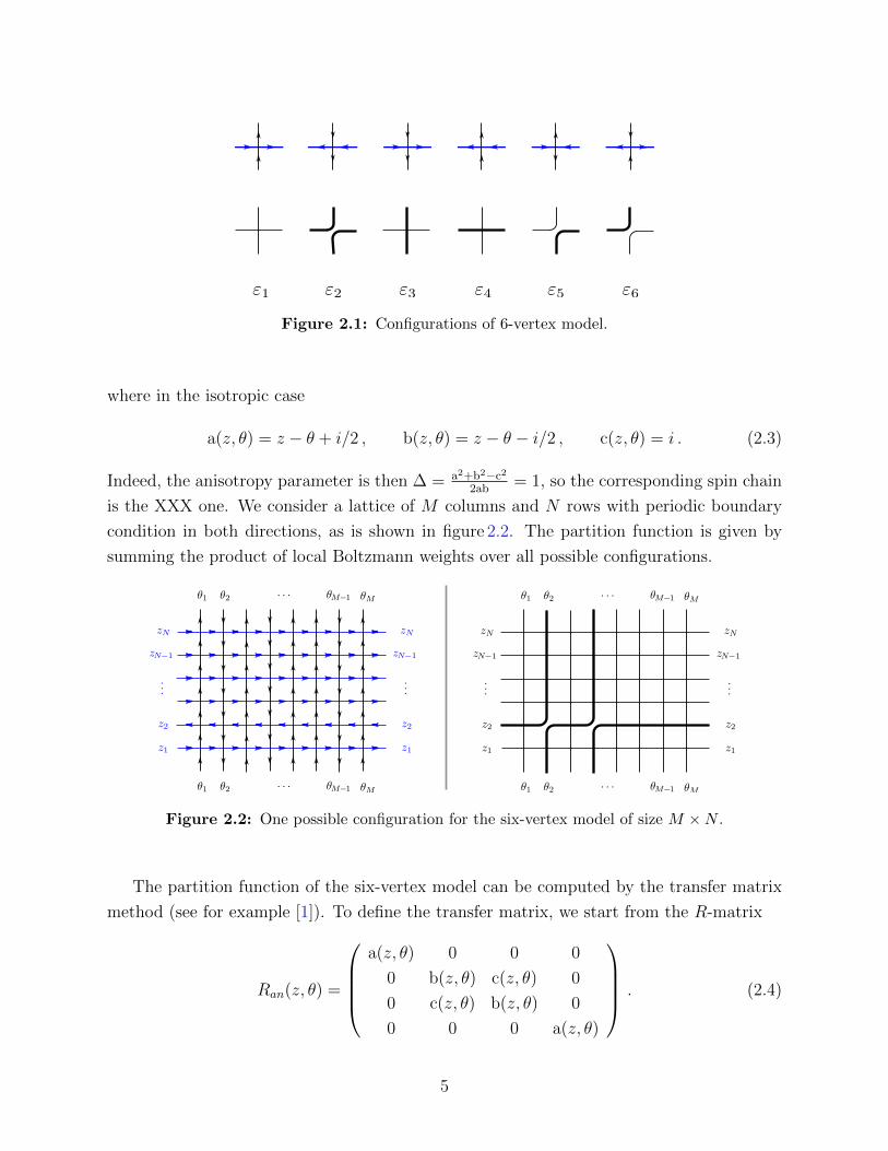
Figure 2.1: Configurations of 6-vertex model.

where in the isotropic case

a(z, θ) = z − θ + i/2 , b(z, θ) = z − θ − i/2 , c(z, θ) = i . (2.3)

Indeed, the anisotropy parameter is then ∆ = a2+b2−c22ab

= 1, so the corresponding spin chain

is the XXX one. We consider a lattice of M columns and N rows with periodic boundary

condition in both directions, as is shown in figure 2.2. The partition function is given by

summing the product of local Boltzmann weights over all possible configurations.

Figure 2.2: One possible configuration for the six-vertex model of size M ×N .

The partition function of the six-vertex model can be computed by the transfer matrix

method (see for example [1]). To define the transfer matrix, we start from the R-matrix

Ran(z, θ) =

a(z, θ) 0 0 0

0 b(z, θ) c(z, θ) 0

0 c(z, θ) b(z, θ) 0

0 0 0 a(z, θ)

. (2.4)

5

Integrability of the six-vertex model is guaranteed by the fact that the R-matrix satisfies

the Yang-Baxter equation

Ran(u)Rbn(v)Rab(u− v) = Rab(u− v)Rbn(v)Ran(u) . (2.5)

The transfer matrix is defined as

TM(z) = Tr a

(M∏n=1

Ran(z, θn)

). (2.6)

The partition function can be written in terms of the transfer matrix

ZM,N = Tr [TM(z1)TM(z2) · · ·TM(zN)] , (2.7)

where the parameters zj and θk characterize the Boltzman weights at each site of the lattice.

We consider the homogeneous case θk = 0 and zj = z. Then the partition function is simply

given by

ZM,N = Tr[TM(z)N

]. (2.8)

It is clear from the above definitions that it is a polynomial of degree MN in the variable

z with rational coefficients.

Transfer matrix. Our task is to compute the trace of TM(z)N . The transfer matrix

TM(z) is a matrix of dimension 2M . The most straightforward way to compute the trace

in (2.8) is by first constructing the matrix explicitly, performing the matrix multiplication

N times and then taking the trace. To simplify this task, it is useful to notice that the

transfer matrix is block-diagonal and we can construct the transfer matrix in each spin

sector separately. The spin sectors are labelled by K where K = 0, 1, . . . ,M is the number

of vertical thick black lines in the right panel of figure 2.2. In the spin chain language, K

corresponds to the number of flipped spins, or the number of magnons with respect to the

pseudo-vacuum state | ↑M〉. The dimension of spin sector K is

dM,K =

(M

K

). (2.9)

We denote the transfer matrix of the spin sector labelled by K as TM,K(z). The partition

function is then given by

ZM,N =M∑K=0

Tr[TM,K(z)N

]. (2.10)

In what follows, we shall call this approach the brute-force method. It serves as a check for

other approaches. This approach becomes cumbersome very quickly since the dimension

dM,K grows rapidly with M and K. For example, d12,6 = 924 which implies that for M = 12

we already need to deal with matrices of dimension about 103.

6

Bethe ansatz. A better method which makes use of the integrability of the model is

the Bethe ansatz. One can diagonalize the transfer matrix by directly constructing its

eigenvectors using Bethe ansatz. The construction can be done in each spin sector. Let

us denote the eigenvectors by |u〉, parameterized by a set of parameters u = {u1, . . . , uK}called rapidities. We then have

TM,K(z)|u〉 = tu(z)|u〉 . (2.11)

Notice that for the spin sector K, the number of rapidities that characterize the state is K.

The eigenvalue tu(z) is given by

tu(z) = a(z)Qu(z − i)Qu(z)

+ d(z)Qu(z + i)

Qu(z), (2.12)

where

a(z) =

(z +

i

2

)M, d(z) =

(z − i

2

)M, (2.13)

and

Qu(z) =K∏j=1

(z − uj) (2.14)

is called the Baxter polynomial. The rapidities are constrained by the Bethe ansatz equations

(BAE) (uj + i/2

uj − i/2

)M=

K∏k 6=j

uj − uk + i

uj − uk − i, j = 1, . . . , K . (2.15)

Bethe ansatz is a very powerful analytical method and it leads to the solution of the

six-vertex model in the thermodynamic limit, when M,N → ∞. However, for fixed and

finite M and N , the expression for tu(z) is only formal since the parameters {u1, . . . , uK}are not known explicitly. To find them, we need to solve the system of algebraic equations

(2.15).

This raises some serious problems if we want to compute the partition function exactly

and explicitly as a polynomial in z. First of all, the BAE for generic M and K are impossible

to solve analytically and can only be solved numerically. Even finding the numerical

solutions turns out to be a highly non-trivial task. Worse, not all the solutions of the

the BAE lead to true eigenvectors and eigenvalues of the transfer matrix. We know that

within each spin sector labelled by K, the dimension of the transfer matrix is dM,K . One

therefore needs to show that there are exactly dM,K physical solutions of the BAE for fixed

M and K. This is intimately related to the completeness problem of Bethe ansatz and is

quite subtle.

7

Physical solutions of the BAE. In general, the number of solutions to the BAE is

more than the number of physical states. It is a non-trivial problem to characterize physical

solutions of BAE among all the solutions. Fortunately, this problem has been studied

systematically in [10]. The conclusion is that the physical solutions can be classified as

pairwise distinct non-singular solutions and singular physical solutions. For a detailed

discussion of these solutions, we also refer to [2]. To single out these solutions, one needs to

impose further constraints in addition to the original set of BAE [2, 10].

To find the physical solutions, it is actually more convenient to work with other formu-

lations of the BAE, in particular Baxter’s TQ-relation and the rational Q-system. Baxter’s

Q-operator provides a powerful method for solving integrable lattice models [1]. The central

equation of this method is an operator equation called the TQ-relation. In terms of the

eigenvalues of the T and Q operators, the TQ relation becomes the following functional

equation

t(z)Q(z) = a(z)Q(z − i) + d(z)Q(z + i) . (2.16)

Note that this equation is basically equivalent to (2.12) if we multiply both sides of the latter

by Qu(z). For a state of length M and magnon number K, t(z) and Q(z) are polynomials

in the variable z of degree M and K, respectively. To solve the TQ-relation (2.16), one first

writes t(z) and Q(z) in the explicit polynomial form

t(z) =M∑j=0

tjzj, Q(z) = zK +

K−1∑k=0

skzk . (2.17)

The unknown variables that we are solving for are {t0, . . . , tM , s0, . . . , sK−1}. Plugging (2.17)

and the explicit form (2.13) of a(z), d(z) into the equation (2.16) and demanding that it

is satisfied for any value of z, one obtains a system of algebraic equations for the unknown

variables. These equations are linear in both sets of variables {t0, . . . , tM} and {s0, . . . , sK−1}and are easier to solve than the original set of BAE. Solving the TQ-relation gives at the

same time both polynomials t(z) and Q(z). The zeros of Q(z) in turn provide the solution

of the BAE. Another advantage of using the TQ-relation is that it automatically eliminates

the solutions with coinciding rapidities, i.e., the solutions of the TQ-relation lead to pairwise

distinct solutions of the BAE.

Working with the TQ-relation instead of the original BAE is already more efficient for

our purpose. However, the use of the TQ-relation does not eliminate all the unphysical

solutions. Very recently, an even more efficient method has been developed for solving

the BAE which is the rational Q-system approach [11, 12]. In this method, one defines

a rational Q-system associated with a Young tableaux with specific boundary conditions.

8

The configuration of the Young tableaux is related to the length and magnon number of

the Bethe state. By requiring all the Q-functions at the vertices of the Young tableaux

to be polynomials, one ends up with a set of algebraic equations called zero-remainder

conditions (ZRC) where the unknown coefficients are the coefficients of the Q-functions,

i.e., the analogues of the {s0, . . . , sK−1} defined above. Solving the Q-system amounts to

finding all the Q-polynomials on the Young tableaux. One specific Q-polynomial coincides

with Q(z) defined above, so its zeros give the Bethe roots. For more details of this approach

and some explicit examples, we refer to appendix A.

It turns out that solving the ZRC is even more efficient than solving the TQ-relation.

Moreover, the solutions of the ZRC are in one-to-one correspondence with the physical

solutions of the BAE, so no further constraints need to be imposed. One minor disadvantage

of this method is that the equations themselves are not known explicitly for any length and

magnon numbers and have to be derived case by case. This is not a big issue in practice

since the equations can be generated rather efficiently for not too large M and K.

In what follows, to find all the physical solutions of the BAE, we will work with rational

Q-systems. So far, the Q-system approach for BAE has only been developed for the isotropic

limit (∆ = 1) corresponding to the XXX spin chain. To treat the XXZ spin chain at generic

∆, we still need to rely on the TQ-relation, together with additional constraints to select

physical solutions. The strategy is to first find the Q-polynomial, and next use the TQ-

relation to find the t-polynomials. After finding all the t-polynomials, it is straightforward

to write down the torus partition function that we are after.

However, it is clear that if we want to find all the t-polynomials explicitly, no matter

which approach (BAE, TQ-relation, Q-system) we are using, we have to solve the system

of algebraic equations numerically. The results are thus approximate and not exact. To

avoid solving equations and obtain instead exact and analytical results for the partition

function, we can however apply methods in computational algebraic geometry. We discuss

these approaches in the next section.

3 Algebro-geometric approach to the partition func-

tion

In this section, we describe our method for computing the torus partition function using an

algebro-geometric approach. The main tools that we are going to use are Grobner basis,

quotient ring and companion matrix. See [13] for a textbook reference to the corresponding

mathematics. For a detailed introduction to these notions in the context of Bethe ansatz,

9

we refer to [2].

As discussed in the previous section, in order to select all the physical solutions, we work

with the rational Q-system. For the su(2) invariant XXX spin chain which is equivalent to

the six-vertex model, the corresponding Young tableaux have two rows with the number of

boxes being (M−K,K). The Q-polynomial that we are interested is Q0,1. The computation

of the Q-polynomials relies on the definition of certain paths on the Young tableau (for more

details, see appendix A). For the su(2) case, we can choose the path such that the unknown

coefficients are precisely the coefficients of Q0,1(z), and we have

Q(z) = Q0,1(z) = zK +K−1∑k=0

sk zk . (3.1)

Ideal. The zero-remainder conditions (ZRC) then give a set of algebraic equations for the

K variables {s0, . . . , sK−1},

f1(s0, s1, · · · , sK−1) = f2(s0, s1, · · · , sK−1) = fS(s0, s1, · · · , sK−1) = 0 , (3.2)

where fk(s0, s1, · · · , sK−1) are polynomials in the variables {s0, · · · , sK−1}. Here S is the

number of equations and it depends on the path we choose. The polynomials f1, · · · , fSdefine an ideal in the polynomial ring C[s0, s1, · · · , sK−1], denoted

IM,K = 〈f1, · · · , fS〉. (3.3)

A given ideal can be generated by different bases, among which the so-called Grobner basis

is particularly useful for us. We denote the Grobner basis by Gk

IM,K = 〈f1, · · · , fS〉 = 〈G1, · · · ,GS′〉 (3.4)

where in general S and S ′ are different. Notice that when computing the Grobner basis we

need to choose a partial ordering of the monomials formed of the variables {s0, s1, · · · , sK−1}.For different orderings, the corresponding Grobner basis can look quite different.

Quotient ring. The quotient ring is defined as

QM,K = C[s0, s1, · · · , sK−1]/IM,K , (3.5)

and it is a finite-dimensional linear space. The dimension of this linear space equals the

number of physical solutions of the BAE for given M and K, which is given by [10]

NM,K =

(M

K

)−(

M

K − 1

). (3.6)

10

Since QM,K is a linear space, it can be spanned by a basis set. The standard basis of the

quotient ring QM,K is given by all the monomials of {s0, · · · , sK−1} that cannot be divided

by LT[Gk] (k = 1, · · · , S ′) where “LT” stands for the leading term in some given partial

ordering. In order to construct the standard basis, one needs to calculate the Grobner basis

of the ideal 〈f1, · · · , fS〉. This is one of the main calculations of the current work which can

be done by standard algorithms such as Buchberger’s algorithm or the F4/F5 algorithm

of Faugere [14, 15]. These algorithms are implemented in several packages for algebraic

geometry, such as Singular [16] .

Companion matrix. Let us denote the basis of the quotient ring by {e1, e2, · · · , eNM,K}.Any polynomial P (s0, s1, . . . , sK−1) can be mapped to a numerical matrix MP called the

companion matrix of dimensionNM,K . The algorithm for doing so is as follows. We multiply

the polynomial P by one of the standard basis elements ej and then find the remainder of

the polynomial reduction with respect to the Grobner basis,

P ej =S′∑k=1

ak Gk + rj . (3.7)

The remainder rj(s0, · · · , sK−1) can be expanded in terms of the standard basis where the

coefficients of the expansion are the elements of the companion matrix, i.e.,

rj =

NM,K∑k=1

Mjk ek , MP = (Mij) . (3.8)

The companion matrix satisfies the following homomorphism properties

MP1±P2 = MP1 ±MP2 ,

MP1P2 = MP1 ·MP2 , (3.9)

MP1/P2 = MP1 ·M−1P2.

The main result from algebraic geometry which we are going to use is∑sol

P (s0, · · · , sK−1) = Tr MP , (3.10)

where the sum ‘sol’ is over all solutions of the system of equations (3.2). It is straightforward

to see that if we start with equations whose coefficients are in Q, the right-hand side of (3.10)

is rational (viz., it is a polynomial in z with rational coefficients), even though individual

terms appearing on the left-hand side may be irrational.

11

Using the procedure described above, after the construction of quotient ring, we can

map the function Q0,1(z) into a companion matrix by mapping each coefficient sk 7→ Sk, so

that

Q0,1(z) 7→ QM,K(z) = zK I +K−1∑k=1

Skzk . (3.11)

where I is the identity matrix of dimension NM,K . Our goal is to find the companion matrix

of the transfer matrix tu(z), since this will permit us to access the partition function. This

can be done by using the explicit expression of the transfer matrix (2.12) and the properties

of the companion matrix (3.9). More explicitly, we have

tu(z) 7→ TM,K(z) , (3.12)

where TM,K(z) can be computed using the ideal generated by the TQ-relations1 or from

the companion matrix QM,K(z) by the following relation

TM,K(z) = [a(z)QM,K(z − i) + d(z)QM,K(z + i)] ·QM,K(z)−1 , (3.13)

valid whenever QM,K(z) is non-singular. The partition function is given by

ZM,N =

[M/2]∑K=0

(M − 2K + 1) Tr(TM,K(z)N

). (3.14)

Several comments are in order. The multiplicities M − 2K + 1, for K ≤M/2, take into

account the descendant states in the Bethe ansatz. These states are obtained by sending

some of the Bethe roots to infinity. It is easy to see that adding a root at infinity does not

change the eigenvalue of the transfer matrix. When solving the BAE or the ZRC, we only

find regular solutions that do not have roots at infinity. Since the descendant states are

indeed part of the spectrum, we need to take them into account in the computation of the

partition function by the proper multiplicity.

The expression in (3.14) takes a very similar form to the one in (2.10). However, there are

important differences. Firstly, the result in (3.14) makes use of the full su(2) symmetry, and

hence the dimensions of the transfer matrices TM,K(z) are smaller than those of TM,K(z).

The dimensions of TM,K(z) and TM,K(z) are NK,M and dK,M respectively, see (3.6) and

(2.9). For example, for M = 14, K = 7, we have N14,7 = 429 and d14,7 = 3432. Therefore

(3.14) is computationally more efficient than (2.10).

1More precisely, to select physical solutions, we need to combine the equations coming from the TQ-

relations and the rational Q-system and then eliminate the variables s.

12

Secondly, one can impose further constraints on the solution space of the BAE and

decompose the solution space into even smaller subspaces for (3.14). This means that we

can make the matrices TM,K(z) in (3.14) block-diagonal and hence work with even smaller

matrices, which improves the efficiency further. This point will be discussed in detail in

section 6.

4 Explicit results

In this section, we give results of partition function for different values of M and N . We

obtain closed-form results up to M = 6 for arbitrary N . The reason we stop at M = 6 is that

the ZRC can be solved analytically up to this length in Q. For M = 7 and M = 8, analytical

solutions of the ZRC can also be found by working in extended fields; see section 6 for more

details. For M ≥ 9, we give an efficient algorithm for computing the partition function

for fixed M and N (which can be large). The results are polynomials in z of high degrees

with rational coefficients (typically large) and it does not make sense to write them down

in this paper. Instead, interested readers can find the results on the repository which we

mentioned in the introduction.

4.1 Closed-form expressions for M ≤ 6

In this section, we list the results for M ≤ 6. We denote the partition function of an M ×Ntoroidal lattice by ZM,N .

M = 1. This is the simplest case. The sum in (3.14) contains only K = 0, and the result

is given by

Z1,N = 2× (2z)N . (4.1)

M = 2. We have to sum over K = 0 and K = 1. The partition function is given by

Z2,N = 3

(2z2 − 1

2

)N+

(2z2 +

3

2

)N. (4.2)

M = 3. We again have to sum over K = 0 and K = 1. The result is

Z3,N = 4

(2z3 − 3

2z

)N+ 2

(2z3 +3

2z +

√3

2

)N

+

(2z3 +

3

2z −√

3

2

)N . (4.3)

13

We see that irrational numbers start to show up within some eigenvalues of the transfer

matrix. However, for any N ∈ N the result for Z3,N is a rational-coefficient polynomial in z

after simplification.

M = 4. We have to sum over K = 0, 1, 2. The result is

Z4,N = 5

(2z4 − 3z2 +

1

8

)N(4.4)

+3

(2z4 + z2 + 2z +

1

8

)N+ 3

(2z4 + z2 − 2z +

1

8

)N+ 3

(2z4 + z2 − 7

8

)N+

(2z4 + 3z2 +

13

8

)N+

(2z4 + 3z2 − 3

8

)N.

M = 5. We have to sum over K = 0, 1, 2. The final result reads

Z5,N = 6

(2z5 − 5z3 +

5

8z

)N(4.5)

+ 4

(2z5 − 1

2

√25 + 10

√5 z2 − 1

8(5− 4

√5)z +

1

8

√5− 2

√5

)N+ 4

(2z5 +

1

2

√25 + 10

√5 z2 − 1

8(5− 4

√5)z − 1

8

√5− 2

√5

)N+ 4

(2z5 − 1

2

√25− 10

√5 z2 − 1

8(5 + 4

√5)z +

1

8

√5 + 2

√5

)N+ 4

(2z5 +

1

2

√25− 10

√5 z2 − 1

8(5 + 4

√5)z − 1

8

√5 + 2

√5

)N+ 2

(2z5 + 3z3 +

21

8z

)N+ 2

(2z5 + 3z3 − 1

2

√10− 2

√5 z2 +

1

8(1 + 4

√5)z − 1

8

√50 + 22

√5

)N+ 2

(2z5 + 3z3 +

1

2

√10− 2

√5 z2 +

1

8(1 + 4

√5)z +

1

8

√50 + 22

√5

)N+ 2

(2z5 + 3z3 − 1

2

√10 + 2

√5 z2 +

1

8(1− 4

√5)z +

1

8

√50− 22

√5

)N+ 2

(2z5 + 3z3 +

1

2

√10 + 2

√5 z2 +

1

8(1− 4

√5)z − 1

8

√50− 22

√5

)N.

We see that the eigenvalues of the transfer matrix now become more complicated, with

double square roots showing up in the coefficients.

14

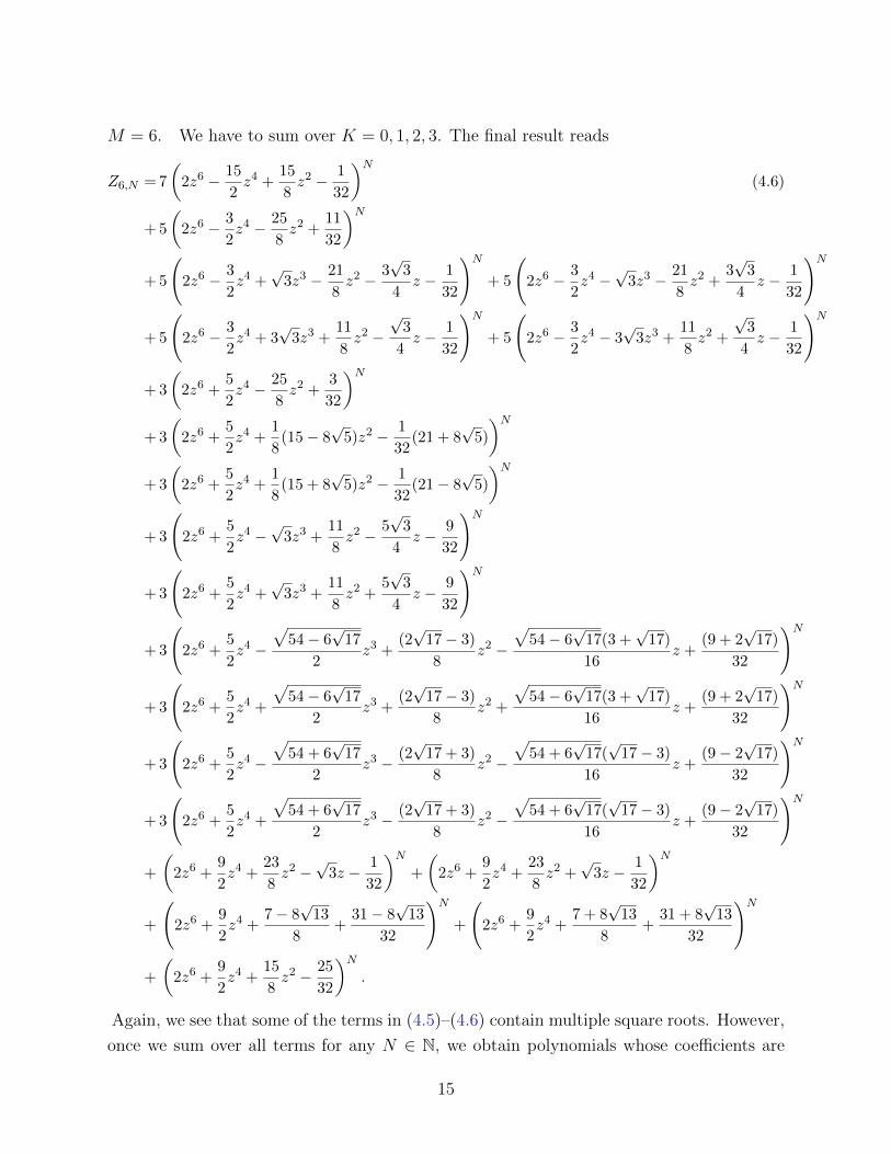
M = 6. We have to sum over K = 0, 1, 2, 3. The final result reads

Z6,N = 7

(2z6 − 15

2z4 +

15

8z2 − 1

32

)N(4.6)

+ 5

(2z6 − 3

2z4 − 25

8z2 +

11

32

)N+ 5

(2z6 − 3

2z4 +

√3z3 − 21

8z2 − 3

√3

4z − 1

32

)N+ 5

(2z6 − 3

2z4 −

√3z3 − 21

8z2 +

3√

3

4z − 1

32

)N

+ 5

(2z6 − 3

2z4 + 3

√3z3 +

11

8z2 −

√3

4z − 1

32

)N+ 5

(2z6 − 3

2z4 − 3

√3z3 +

11

8z2 +

√3

4z − 1

32

)N

+ 3

(2z6 +

5

2z4 − 25

8z2 +

3

32

)N+ 3

(2z6 +

5

2z4 +

1

8(15− 8

√5)z2 − 1

32(21 + 8

√5)

)N+ 3

(2z6 +

5

2z4 +

1

8(15 + 8

√5)z2 − 1

32(21− 8

√5)

)N+ 3

(2z6 +

5

2z4 −

√3z3 +

11

8z2 − 5

√3

4z − 9

32

)N

+ 3

(2z6 +

5

2z4 +

√3z3 +

11

8z2 +

5√

3

4z − 9

32

)N

+ 3

(2z6 +

5

2z4 −

√54− 6

√17

2z3 +

(2√

17− 3)

8z2 −

√54− 6

√17(3 +

√17)

16z +

(9 + 2√

17)

32

)N

+ 3

(2z6 +

5

2z4 +

√54− 6

√17

2z3 +

(2√

17− 3)

8z2 +

√54− 6

√17(3 +

√17)

16z +

(9 + 2√

17)

32

)N

+ 3

(2z6 +

5

2z4 −

√54 + 6

√17

2z3 − (2

√17 + 3)

8z2 −

√54 + 6

√17(√

17− 3)

16z +

(9− 2√

17)

32

)N

+ 3

(2z6 +

5

2z4 +

√54 + 6

√17

2z3 − (2

√17 + 3)

8z2 −

√54 + 6

√17(√

17− 3)

16z +

(9− 2√

17)

32

)N

+

(2z6 +

9

2z4 +

23

8z2 −

√3z − 1

32

)N+

(2z6 +

9

2z4 +

23

8z2 +

√3z − 1

32

)N+

(2z6 +

9

2z4 +

7− 8√

13

8+

31− 8√

13

32

)N+

(2z6 +

9

2z4 +

7 + 8√

13

8+

31 + 8√

13

32

)N

+

(2z6 +

9

2z4 +

15

8z2 − 25

32

)N.

Again, we see that some of the terms in (4.5)–(4.6) contain multiple square roots. However,

once we sum over all terms for any N ∈ N, we obtain polynomials whose coefficients are

15

rational numbers, as expected.

4.2 Partition functions for higher M and N

For M = 7 and M = 8, we can also work out the analytical results. However, the closed-

form results involve complicated multi-square roots and are not very illuminating to write

down explicitly here. For M ≥ 9, we are not able to find analytical solutions anymore. For

these cases, we give an efficient approach to compute the partition function for fixed M and

N based on the companion matrix.

Although our method is much more efficient than the brute-force approach, the com-

plexity still grows exponentially with M . On a laptop, we are able to compute the Grobner

basis and companion matrices of the Q-polynomial Q(z) and the transfer matrix TM,K(z)

up to M = 14 after algebraic extension (see more details in section 6). The dimensions

of the companion matrices with fixed M,K, ` are given in tables 3–15. In general, the

partition function ZM,N(z) is a polynomial of order MN . Let us consider one example and

take M = 14, N = 100. We have

Z14,100(z) =700∑k=0

cnz2n (4.7)

where cn are rational numbers. The full result is too large to show, we present simply

one coefficient, say c50, here just to give an idea about the result. It can be written as

c50 = N50/D50 where N50 and D50 are integers and are given by

N50 = 3549714199509718765414261648405948375346908444631449814070999015959834

5566548305771114077497148041577082024237243782436360433278999500001467

7415020115130416461041186374238411444900889750187515469354178173296042

6263542784005444527370571255655399436082869031810512249627664031748092

4072971596196276059412147685707041129531252668420023067545577282800096

9295580666703059631065928833005677223301695252356346794040665489002919

252969420827675164522054378930548720509758103112303817657569605

16

and

D50 = 5254662920039596746236382353531688074822975081008511328653941899536358

8535283647520133924979358051065937411251928593712733718650179494204788

1824032065695719746688948719970424831685787857667697873122163831147965

2780562037740551931521573661427623891169657954033123606560887017391291

1075991202517005852196882800252419269626961951377918107052351183818088

1989632 .

Approximately this number is c50 ≈ 6.75536× 10125. Using numerical methods such as the

function Rationalize in Mathematica to guess such a large number will be quite difficult

in practice since it requires working with floating point numbers with very high accuracy.

Since the results for partition functions for large N are typically large, we find it

more useful to give the companion matrices. These companion matrices contain all the

information we need. To find the explicit eigenvalues of Qu(z) and tu(z), we can diagonalize

the companion matrices. In general this diagonalization can only be done numerically, but

the matrices that we need to diagonalize are much smaller and can be handled much more

efficiently. The zeros of Qu(z) give the Bethe roots. That is to say, we can straightforwardly

find all physical solutions of the BAE up to lengthM = 14 using our results. The eigenvalues

tu(z) contain all the information about conserved charges of the system, i.e., momentum,

energy and higher conserved charges of the Bethe states.

To find the exact partition function ZM,N , we need to take matrix powers of the compa-

nion matrices TM,K(z)N and then take the trace. We will be interested in the case of large N .

Naively, we would need to perform N matrix multiplications involving the companion matrix

before taking the trace. When the size of the matrix is large, the analytic computation of

matrix multiplication become time consuming. To reach a high value of N , we actually

need a better way to do the computation. This is described in appendix C.

4.3 Consistency check

Since our results are usually large polynomials, it is important to perform some checks for

their correctness. One important consistency check is the following. We can compute the

lattice partition function in two ways, corresponding to two different choices of the transfer

direction, and the result should be the same, as is shown in figure 4.3. Specifically, we

consider the transformation of the partition function where we rotate the lattice by π/2.

To analyze the effect of this transformation, we consider the M ×N lattice with M vertical

17

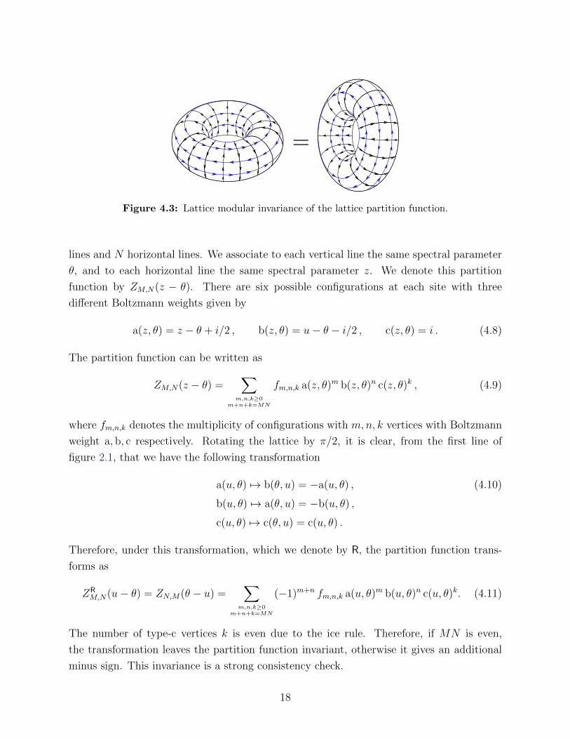
Figure 4.3: Lattice modular invariance of the lattice partition function.

lines and N horizontal lines. We associate to each vertical line the same spectral parameter

θ, and to each horizontal line the same spectral parameter z. We denote this partition

function by ZM,N(z − θ). There are six possible configurations at each site with three

different Boltzmann weights given by

a(z, θ) = z − θ + i/2 , b(z, θ) = u− θ − i/2 , c(z, θ) = i . (4.8)

The partition function can be written as

ZM,N(z − θ) =∑

m,n,k≥0m+n+k=MN

fm,n,k a(z, θ)m b(z, θ)n c(z, θ)k , (4.9)

where fm,n,k denotes the multiplicity of configurations with m,n, k vertices with Boltzmann

weight a, b, c respectively. Rotating the lattice by π/2, it is clear, from the first line of

figure 2.1, that we have the following transformation

a(u, θ) 7→ b(θ, u) = −a(u, θ) , (4.10)

b(u, θ) 7→ a(θ, u) = −b(u, θ) ,

c(u, θ) 7→ c(θ, u) = c(u, θ) .

Therefore, under this transformation, which we denote by R, the partition function trans-

forms as

ZRM,N(u− θ) = ZN,M(θ − u) =

∑m,n,k≥0

m+n+k=MN

(−1)m+n fm,n,k a(u, θ)m b(u, θ)n c(u, θ)k. (4.11)

The number of type-c vertices k is even due to the ice rule. Therefore, if MN is even,

the transformation leaves the partition function invariant, otherwise it gives an additional

minus sign. This invariance is a strong consistency check.

18

We use this relation to check the correctness of the companion matrices as follows.

For a given length M , we construct the corresponding companion matrices and compute

the partition function ZM,N(z − θ) for all N ≤ M . These partition functions can also be

computed as ZN,M(θ − z) using the companion matrices constructed for length N . If the

results are correct, the two calculations should give the same result. We have checked the

companion matrix in this way up to M = 14.

5 Zeros of partition functions

The torus partition function ZM,N(z) is a polynomial of order MN in z. It is instructive to

find the zeros of this partition function in the complex z-plane.

Partition function zeros for statistical models with one complex parameter have been

studied in a variety of contexts—including Lee-Yang zeros (complex magnetic field) [17],

Fisher zeros (complex temperature) [18], and graph polynomials such as the Q-colour

chromatic polynomial [3–9]—and has given rise to an immense literature (see, e.g., references

in [3]). The zeros of partition functions in the thermodynamic limit contain information

about the phases and critical behavior of the model at hand. In many cases the zeros

will accumulate on curves, for M,N → ∞, which “pinch” the real axis at one or more

critical points. Isolated accumulation points provide another possible scenario. In the

simplest cases—such as the Ising model with suitable boundary conditions—the curves of

accumulation points can be proved to form circles, giving rise to so-called circle theorems.

More generally, the density of zeros near a critical point obey scaling laws that can be

related to critical exponents.

The true thermodynamic limit of anM×N system is obtained by lettingM,N →∞ with

a fixed and finite ratio, 0 < M/N <∞. But another means of obtaining relevant information

is to fix a finite value of M , and study the accumulation points of zeros as N →∞. For a

partition function of the form (3.14), and supposing a mild non-degeneracy condition, the

Beraha-Kahane-Weiss theorem [19] states that the accumulation points will form curves. By

standard analyticity theorems, any closed region delimited by such curves will constitute

a thermodynamical phase (for N → ∞). Under reasonable (but not entirely innocuous)

assumptions about the commutativity of limits, the phase diagram in the thermodynamic

limit can then be inferred by studying the convergence of these curves upon taking M →∞.

19

5.1 Partition functions for different M and N

In this subsection, we give the partition function zeros for different M and N . We fix the

value of M and increase N to see how the distribution of the zeros change. In this way, we

try to extrapolate the behaviors of the zeros to the (partial) thermodynamic limit N →∞(with M being fixed and finite). One might wonder what is the benefit of knowing the

partition function exactly for finding the zeros. Naively one might expect that numerical

approximations will be sufficient for finding the zeros of the partition function. However, it

is known that the locations of zeros of a polynomial can be very sensitive to perturbations

of coefficients, especially when the degree of the polynomial is large. One famous example

is the so-called Wilkinson’s polynomial where a change of one of the coefficients by 10−7

leads to significant changes in the locations of the zeros. Having exact results eliminates

this potential subtlety.

In figure 5.4 we show the partition function zeros for M = 4, 5, · · · , 8 with various

aspect ratios, namely N = ρM for ρ = 10, 20, 40, 80 (and in one case ρ = 160). The lower

right corner shows the result of out largest computation with M = 14 and N = 100. The

partition functions for M = 4, 5, 6 have been computed by the direct application of the

explicit formulae (4.4)–(4.6), and the remaining results by the algebro-geometric method.

These are polynomials of degree MN , and the coefficients can be normalized to be integers

by multiplying ZM,N(z) by the overall factor 2(M−1)N . Given the very large degree and

the size of their coefficients, it is actually a non-trivial task to compute the zeros of these

polynomials. These difficulties are however efficiently overcome by the application of the

software MPSolve [20], which is a multiprecision implementation of the Aberth method

[21]. The main advantage of the latter method is that it approximates all the roots of a

univariate polynomial simultaneously.

The zero plots in figure 5.4 reveal several interesting features. As the aspect ratio ρ

grows, the zeros tend to settle on certain curves—the limiting curves of accumulation points

to be discussed further in the next subsection. In the regions close to the origin the finite-ρ

effects are small, but further away their importance increases, and the fine structure of the

limiting curves are barely visible even at the largest ρ shown. Moreover, far from the origin

the density of zeros is very scarce. Regarding the case M = 14, it seems likely that it would

develop rich details as those seen in the other plots, provided large ρ could be accessed. In

particular, there are “stray” zeros around the central almost-horizontal branches that appear

as precursors of multiple branches and T-points. While all these features could certainly be

analyzed at length, we instead move on to the direct determination of the limiting curves

as ρ→∞.

20

-4

-2

0

2

4

-4 -2 0 2 4

M=4, N=40M=4, N=80

M=4, N=160M=4, N=320

-4

-2

0

2

4

-4 -2 0 2 4

M=5, N=50M=5, N=100M=5, N=200M=5, N=400M=5, N=800

-4

-2

0

2

4

-4 -2 0 2 4

M=6, N=60M=6, N=120M=6, N=240M=6, N=480

-4

-2

0

2

4

-4 -2 0 2 4

M=7, N=70M=7, N=140M=7, N=280M=7, N=560

-4

-2

0

2

4

-4 -2 0 2 4

M=8, N=80M=8, N=160M=8, N=320M=8, N=640

-4

-2

0

2

4

-4 -2 0 2 4

M=14, N=100

Figure 5.4: Partition function zeros in the complex z-plane, shown in reading direction for

M = 4, 5, · · · , 8 and M = 14.

21

5.2 Limiting curves

In the previous subsection, we have seen that as N increases, the zeros of the partition

function accumulate on some curves. Following [3] we shall refer to these as limiting curves.

By the Beraha-Kahane-Weiss (BKW) theorem [19], this is a consequence of the form (2.10),

or equivalently of (3.14), that relates the partition function ZM,N to sum over traces of

the N ’th power of the transfer matrix TM,K(z), or of the corresponding companion matrix

TM,K(z) given by (3.12).

More precisely, the BKW theorem applies to an expression of the form

ZM,N(z) =∑i

αi(z)Λi(z)N , (5.1)

where we shall refer to the Λi(z) as eigenvalues, and the αi(z) as the corresponding multi-

plicities. For a given z, let us order the eigenvalues by norm, so that |Λ1(z)| ≥ |Λ2(z)| ≥· · · , and we call an eigenvalue Λi(z) dominant (at z) if its norm is maximal, |Λi(z)| ≤|Λ1(z)|. Supposing a mild non-degeneracy condition, the BKW theorem then states that

the accumulation set of zeros, as N → ∞, will form either isolated points or curves. An

isolated accumulation point occurs for z = z0, when there is a unique dominant eigenvalue

(i.e., |Λ1(z0)| > |Λ2(z0)|) and the corresponding multiplicity vanishes (i.e., α1(z0) = 0). A

curve of accumulation points occurs when there are at least two dominant eigenvalues (i.e.,

|Λ1(z)| = |Λ2(z)|), and the relative phase φ(z) ∈ R defined by Λ2(z) = eiφ(z)Λ1(z) varies

along the curve. The speed of variation of φ(z) along the curves can be related to the

density of partition function zeros [3]. Note also that the limiting curves may have T-points

or higher-order bifurcations at a point z0 where more than two eigenvalues are equimodular.

We refer to [3] for more details on the BKW theorem and the detailed analysis of the generic

setup.

In our context, αi(z) and Λi(z) depend on M and K, and moreover αi(z) = M −2K+ 1

are simply constants. Therefore all accumulation points form curves, and not isolated points,

in agreement with the observations of the preceding subsection. To trace these curves for

a given M , we use an approach for identifying the loci of equimodularity that is described

in appendix D. This consists in two steps: first we identify some points of equimodularity

by a direct search (e.g., along suitably chosen straight lines), and second we trace the

equimodular curves starting from each of those points, using a procedure explained in the

appendix. While this approach may fail to detect very small curves of accumulation points,

we believe to have obtained complete results for M ≤ 8.

The resulting limiting curves for M = 4, 5, · · · , 8 are shown in figure 5.5. A number

of qualitative features can be read off from these examples. First, the curves are invariant

22

-4

-2

0

2

4

-4 -2 0 2 4

M=4

-4

-2

0

2

4

-4 -2 0 2 4

M=5

-4

-2

0

2

4

-4 -2 0 2 4

M=6

-4

-2

0

2

4

-4 -2 0 2 4

M=7

-4

-2

0

2

4

-4 -2 0 2 4

M=8

Figure 5.5: Limiting curves of accumulation points of partition function zeros in the complex

z-plane, shown in reading direction for M = 4, 5, · · · , 8.

23

under the independent sign changes of Re z and Im z. Second, they all contain the point

z = i/2. Third, they contain a number of branches extending to infinity; the number of such

branches within each quadrant appears to be 3, 3, 5, 4, 7 for the sizes considered. Fourth,

for even M the curves do not intersect the real axis, while for odd M they contain an exact

vertical ray z ∈ [−i/2, i/2]. For odd M , there are further intersections with the real axis,

namely z ' ±3.5970 for M = 5, as well as z ' ±3.0096 and z ' ±6.0139 for M = 7. Fifth,

we only find T-points and now higher-order bifurcations.

-1

-0.5

0

0.5

1

0 0.5 1 1.5 2 2.5 3 3.5

M=5M=7M=9

M=11M=13M=15M=17

0.00 0.05 0.10 0.15 0.202.0

2.5

3.0

3.5

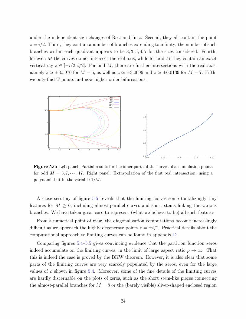
Figure 5.6: Left panel: Partial results for the inner parts of the curves of accumulation points

for odd M = 5, 7, · · · , 17. Right panel: Extrapolation of the first real intersection, using a

polynomial fit in the variable 1/M .

A close scrutiny of figure 5.5 reveals that the limiting curves some tantalizingly tiny

features for M ≥ 6, including almost-parallel curves and short stems linking the various

branches. We have taken great case to represent (what we believe to be) all such features.

From a numerical point of view, the diagonalization computations become increasingly

difficult as we approach the highly degenerate points z = ±i/2. Practical details about the

computational approach to limiting curves can be found in appendix D.

Comparing figures 5.4–5.5 gives convincing evidence that the partition function zeros

indeed accumulate on the limiting curves, in the limit of large aspect ratio ρ → ∞. That

this is indeed the case is proved by the BKW theorem. However, it is also clear that some

parts of the limiting curves are very scarcely populated by the zeros, even for the large

values of ρ shown in figure 5.4. Moreover, some of the fine details of the limiting curves

are hardly discernable on the plots of zeros, such as the short stem-like pieces connecting

the almost-parallel branches for M = 8 or the (barely visible) sliver-shaped enclosed region

24

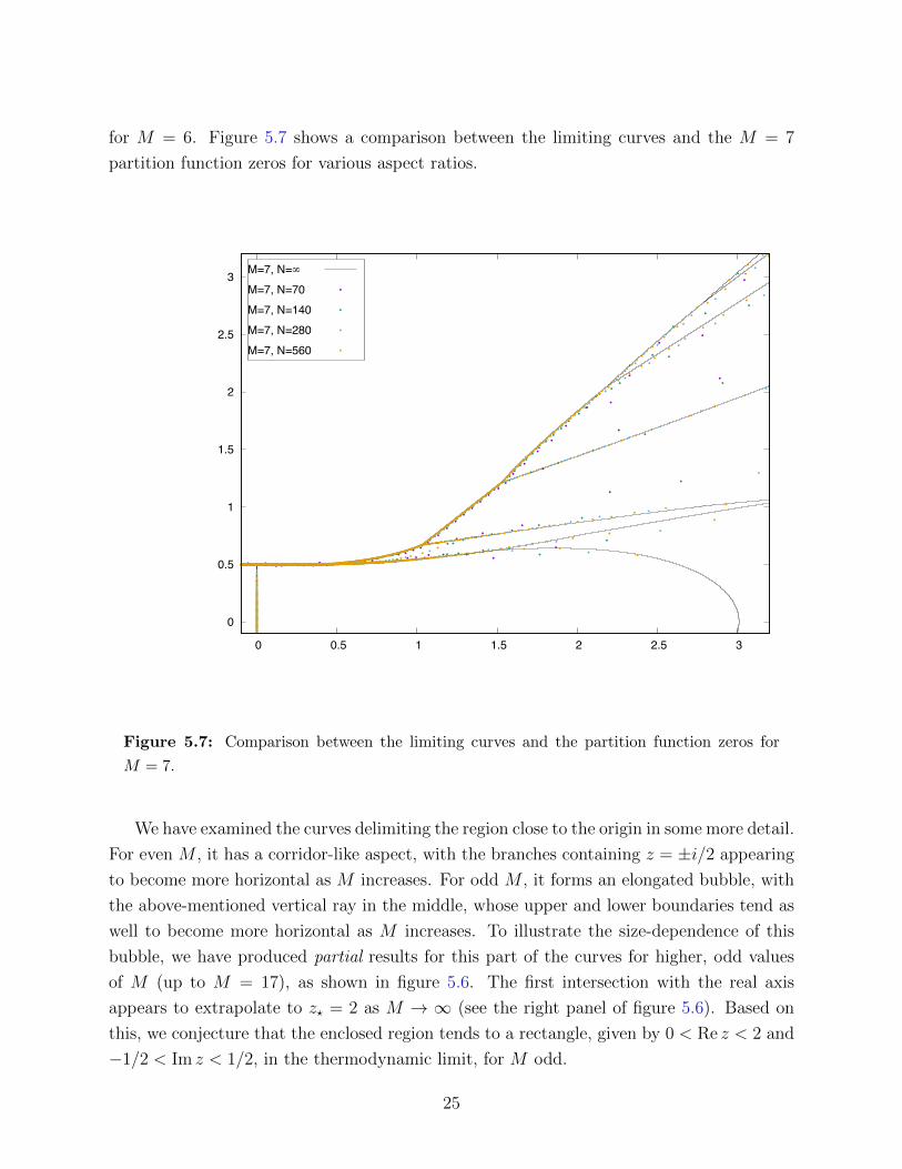
for M = 6. Figure 5.7 shows a comparison between the limiting curves and the M = 7

partition function zeros for various aspect ratios.

0

0.5

1

1.5

2

2.5

3

0 0.5 1 1.5 2 2.5 3

M=7, N=∞M=7, N=70M=7, N=140M=7, N=280M=7, N=560

Figure 5.7: Comparison between the limiting curves and the partition function zeros for

M = 7.

We have examined the curves delimiting the region close to the origin in some more detail.

For even M , it has a corridor-like aspect, with the branches containing z = ±i/2 appearing

to become more horizontal as M increases. For odd M , it forms an elongated bubble, with

the above-mentioned vertical ray in the middle, whose upper and lower boundaries tend as

well to become more horizontal as M increases. To illustrate the size-dependence of this

bubble, we have produced partial results for this part of the curves for higher, odd values

of M (up to M = 17), as shown in figure 5.6. The first intersection with the real axis

appears to extrapolate to z? = 2 as M → ∞ (see the right panel of figure 5.6). Based on

this, we conjecture that the enclosed region tends to a rectangle, given by 0 < Re z < 2 and

−1/2 < Im z < 1/2, in the thermodynamic limit, for M odd.

25

6 Primary decomposition

Let us summarize what we have achieved so far in computing the torus partition function

of the six-vertex model. Computing the partition function by brute force, we need to work

with matrices of dimension dM,K within the spin sector of K magnons. Using Bethe ansatz

and the algebro-geometric method, we are able to reduce the problem to the computation of

companion matrices of dimension NM,d = dM,K − dM,K−1. This reduction in the dimensions

of the matrices makes use of the full su(2) symmetry of the theory. Recall that we classify

the Bethe states as primary states and their descendants with respect to the su(2) algebra.

Since all the descendant states of a given primary state have the same eigenvalue of the

transfer matrix, we can focus on the primary states only. The number of primary states is

much less than the total number of states in a given spin sector.

Can we do better? Notice that we have not yet exploited all the symmetries of the

model. For example, the model is also invariant under a lattice translation. This symmetry

leads to the the total momentum of the Bethe state being quantized, taking only a finite

number of possible values. Therefore, apart from decomposing the Hilbert space according

to spin sectors, we can also decompose the Hilbert space according to momentum sectors,

i.e., states with different values of the lattice momentum. These two decompositions can be

performed simultaneously and leads to even smaller companion matrices. This will greatly

enhance the efficiency of our approach.

Mathematically, the decomposition with respect to momentum sectors is intimately

related to primary decomposition and algebraic extension in algebraic geometry. Physically,

this decomposition also allows us to probe much deeper into the solution space of BAE

and find new structures that have not been studied in the literature. In this section, we

discuss the decomposition of the solution space with respect to momentum sectors. We first

introduce the notion of primary decomposition on Q from some interesting observations

about the partition function. We will see that it is useful to perform the decomposition on a

larger field Q(i, ξM) obtained by an algebraic extension. In addition, exploiting Galois theory

in the current context, we will show that many of the subspaces after the decomposition are

actually related by the Galois group, and it is thus sufficient to perform the computation

for a representative. The decomposition together with Galois theory lead to a huge boost in

the efficiency of our computation. More details are given in appendix B and an upcoming

publication [22].

26

6.1 Primary decomposition over Q

To see that the solution space of the BAE has more structure, we take a careful look at the

closed-form results of the partition function in (4.6). We can see that it is natural to group

some of the terms together since they take very similar forms. For example, we can group

the following four eigenvalues in (4.6):

Λ1 = 2z6 +5

2z4 −

√54− 6

√17

2z3 +

(2√

17− 3)

8z2 −

√54− 6

√17(3 +

√17)

16z +

(9 + 2√

17)

32, (6.1)

Λ2 = 2z6 +5

2z4 +

√54− 6

√17

2z3 +

(2√

17− 3)

8z2 +

√54− 6

√17(3 +

√17)

16z +

(9 + 2√

17)

32,

Λ3 = 2z6 +5

2z4 −

√54 + 6

√17

2z3 − (2

√17 + 3)

8z2 −

√54 + 6

√17(√

17− 3)

16z +

(9− 2√

17)

32,

Λ4 = 2z6 +5

2z4 +

√54 + 6

√17

2z3 − (2

√17 + 3)

8z2 −

√54 + 6

√17(√

17− 3)

16z +

(9− 2√

17)

32.

One can check that although each Λ1, · · · ,Λ4 is complicated and has irrational coefficients

for generic z, their symmetric power sums

Λn1 + Λn

2 + Λn3 + Λn

4 (6.2)

are always polynomials whose coefficients are rational numbers! Since each Λi corresponds

to a solution of the BAE or the TQ-relation, this implies that we can group the four

corresponding solutions of the BAE. Notice that we cannot make the decomposition further

on Q. If we further divide the four solutions into two groups, say Λ1,Λ2 and Λ3,Λ4, then the

coefficients of the symmetric power sums Λn1 + Λn

2 and Λn3 + Λn

4 are no longer rational. This

implies that these four solutions form an irreducible or primary block on Q. Similarly, the

remaining terms in (4.6) can be divided into such primary blocks. In geometrical terms, this

grouping is equivalent to decomposing an affine variety into independent components. Such

an operation is called primary decomposition in algebraic geometry. We refer to appendix B

for more details.

Given an ideal, it is straightforward to compute the primary decomposition using stan-

dard algorithms. To understand the physical meaning of primary decomposition, we now

analyze the example M = 6 carefully.

An example: M = 6. The result of the primary decomposition is given in table 1. Let us

consider the spin sector K = 2. From table 1 we see that there are 9 physical solutions for

M = 6, K = 2, and that these solutions can be divided into four groups, with dimensions

1,2,2,4. In particular, the dimension-4 subspace corresponds to the four eigenvalues given

in (6.1).

27

K M = 6

1 5=1+2+2

2 9=1+2+2+4

3 5=1+2+2

Table 1: Primary decomposition of solution space of BAE with M = 6. The numbers on the

right-hand sides of each line represent the dimension of each subspace.

As we alluded to before, this decomposition is related to the lattice translational invari-

ance which is generated by the shift operator U = eiP . As an operator, it is related to the

transfer matrix as

UM = (−i)MTM(i/2). (6.3)

For a closed spin chain of length M , the allowed eigenvalues of the shift operator are

exp

(2πi`

M

), ` = 1, · · · ,M. (6.4)

Let us denote the four subspaces as A,B,C,D; we can then compute the values of ` for

M = 6 for each subspace. The result is shown in table 2. We see that the value of ` is

dimensions values of ` eigenvalues of U3

A 1 {3} −1

B 2 {6, 6} +1

C 2 {1, 5} −1

D 4 {2, 2, 4, 4} +1

Table 2: The values of ` and eigenvalues of U3 for physical solutions of BAE with M =

6,K = 2 in the four subspaces under primary decomposition. All the solutions in the same

subspace have the same eigenvalues of U3.

not the same within each subspace. However, if we compute the eigenvalues of the operator

U3, we find that they are the same within each subspace, as is shown in the last column of

table 2. This is due to the fact that we work on the field Q. Let us denote ξM = exp(2πi/M).

It is clear that ξ`M is not always rational for all ` = 1, · · · ,M . Therefore one cannot perform

the decomposition over momentum sector completely on Q. For each M , we can find the

smallest integer 1 ≤ m ≤ M such that the all the eigenvalues of Um are rational. Then

we can perform the decomposition with respect to the eigenvalues of Um. As a result, we

28

can restrict ourselves to each subspace by imposing an additional constraint on the original

BAE. In our example, for M = 6, K = 2, the additional constraints for the four subspaces

are

A : U = (−i)6t(i/2) = −1, (6.5)

B : U = (−i)6t(i/2) = +1,

C : U3 =[(−i)6t(i/2)

]3= −1, U = (−i)6t(i/2) 6= −1,

D : U3 =[(−i)6t(i/2)

]3= +1, U = (−i)6t(i/2) 6= +1.

Notice that we need to include the constraints U 6= ±1 in the cases C and D because

otherwise they will include cases A and B.

Algebraic extension. As we see in the previous discussion, the primary decomposition is

related to the decomposition with respect to the lattice momentum. Due to the fact that ξ`Mis not always a rational number, we cannot perform the decomposition completely. However,

we are not constrained to work on the field Q. If we extend the field slightly to include ξM

and perform the primary decomposition on the extended field, then the decomposition with

respect to the lattice momentum can be performed completely. More precisely, the extended

field will turn out to be FM = Q(i, ξM) where i is the imaginary unit.

After the decomposition into momentum sectors, we have M subspaces2 (corresponding

to ` = 1, · · · ,M) in each spin sector K. In principle, we need to compute the Grobner

basis and companion matrices of all subsystems. However, we will show that by making use

of the Galois group of the algebraic extension, we just need to calculate a very few BAE

subsystems. We get the contribution from all subsystems by the Galois group actions.

6.2 Primary decomposition over FM

We explain in detail how to implement the decomposition over FM in practice. Since we

work with the rational Q-system, it is most convenient to express the momentum condition

in terms of Baxter polynomials Q(z) as

K∏j=1

uj + i/2

uj − i/2=Qs(−i/2)

Qs(+i/2)= ξ`M , ` = 1, · · · ,M . (6.6)

2Some of the subspaces might not exist for some values of M and K, as witnessed by the tables in the

next subsection.

29

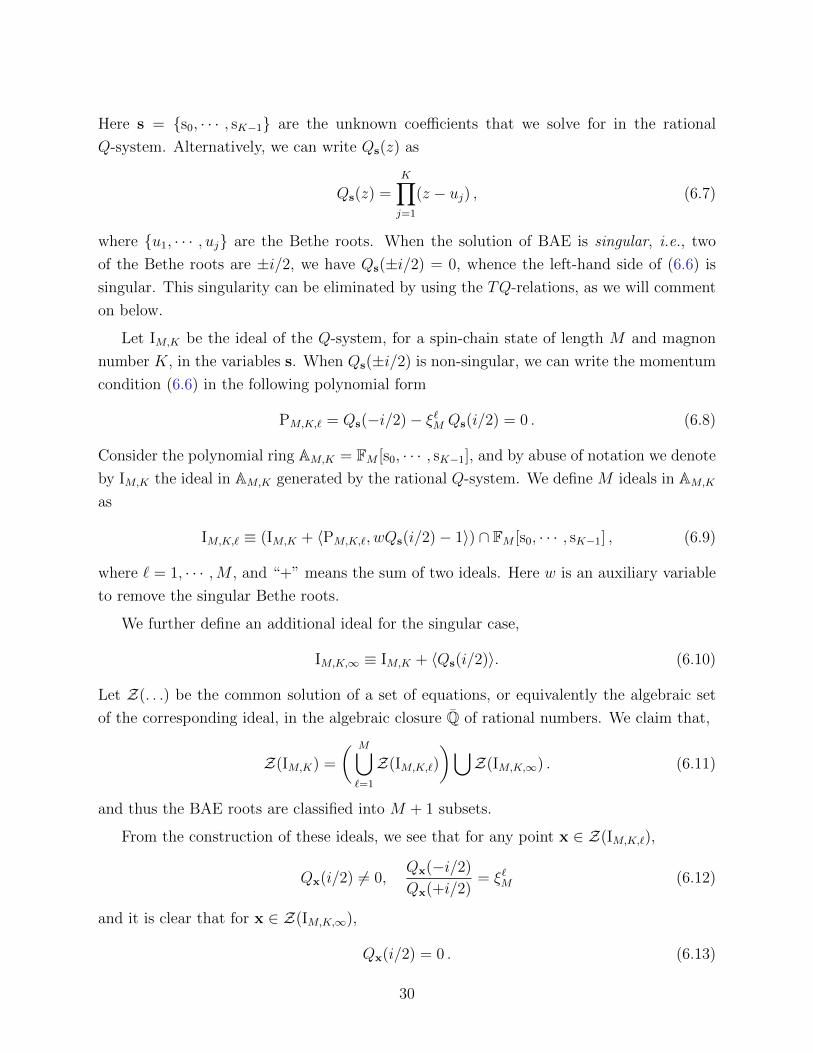
Here s = {s0, · · · , sK−1} are the unknown coefficients that we solve for in the rational

Q-system. Alternatively, we can write Qs(z) as

Qs(z) =K∏j=1

(z − uj) , (6.7)

where {u1, · · · , uj} are the Bethe roots. When the solution of BAE is singular, i.e., two

of the Bethe roots are ±i/2, we have Qs(±i/2) = 0, whence the left-hand side of (6.6) is

singular. This singularity can be eliminated by using the TQ-relations, as we will comment

on below.

Let IM,K be the ideal of the Q-system, for a spin-chain state of length M and magnon

number K, in the variables s. When Qs(±i/2) is non-singular, we can write the momentum

condition (6.6) in the following polynomial form

PM,K,` = Qs(−i/2)− ξ`M Qs(i/2) = 0 . (6.8)

Consider the polynomial ring AM,K = FM [s0, · · · , sK−1], and by abuse of notation we denote

by IM,K the ideal in AM,K generated by the rational Q-system. We define M ideals in AM,K

as

IM,K,` ≡ (IM,K + 〈PM,K,`, wQs(i/2)− 1〉) ∩ FM [s0, · · · , sK−1] , (6.9)

where ` = 1, · · · ,M , and “+” means the sum of two ideals. Here w is an auxiliary variable

to remove the singular Bethe roots.

We further define an additional ideal for the singular case,

IM,K,∞ ≡ IM,K + 〈Qs(i/2)〉. (6.10)

Let Z(. . .) be the common solution of a set of equations, or equivalently the algebraic set

of the corresponding ideal, in the algebraic closure Q of rational numbers. We claim that,

Z(IM,K) =

( M⋃`=1

Z(IM,K,`)

)⋃Z(IM,K,∞) . (6.11)

and thus the BAE roots are classified into M + 1 subsets.

From the construction of these ideals, we see that for any point x ∈ Z(IM,K,`),

Qx(i/2) 6= 0,Qx(−i/2)

Qx(+i/2)= ξ`M (6.12)

and it is clear that for x ∈ Z(IM,K,∞),

Qx(i/2) = 0 . (6.13)

30

Hence, for different ` ∈ {1, . . .M,∞}, the algebraic sets Z(IM,K,`) have no intersection, so

the union (6.11) is disjoint. Since the Q-system equation has no coinciding Bethe roots by

construction, IM,K,` are all radical ideals. By Hilbert’s Nullstellensatz,

IM,K =

( M⋂`=1

IM,K,`

)⋂IM,K,∞ . (6.14)

This is the ideal decomposition which is crucial for the efficient computation of exact

partition function via Grobner bases. Note that in this paper, we do not prove that for

` ∈ {1, . . . ,M,∞}, each IM,K,` is primary over the field FM , i.e., that there exists no further

decomposition beyond the computation in this paper. This discussion is left for future work.

Another comment is that one may well expect that in addition to the lattice translation

symmetry, there can be other discrete symmetries such as reflection symmetry that may

play a similar role. Namely, we can further decompose the solution space with respect to

these symmetries. This interesting possibility is also left for future work.

With the decomposition (6.11), the exact partition function is presented as a sum over

the contributions from the ideals in (6.14),

ZM,N(z) =

bM/2c∑K=0

(M − 2K + 1)

∑`∈{1,...M,∞}

Tr (TM,K,`(z)N)

, (6.15)

where the companion matrix TM,K,`(z) is the companion matrix for(a(z)QM,K(z − i) + d(z)QM,K(z + i)

)QM,K(z)−1 (6.16)

in the ideal IM,K,`. Note that TM,K,`(z) contains polynomials in i and ξM but no other

algebraic numbers. As we will see, each TM,K,l(z) has a much smaller size than the original

companion matrix TM,K(z), hence (6.15) provides a highly efficient way of computing the

partition function.

Finally, we comment on the Bethe roots in IM,K,∞, i.e., singular roots. The singularity

of the eigenvalue of U in terms of Qs(±i/2) is actually spurious. They can be eliminated

by using the TQ-relation. We can combine the equations from the rational Q-system and

the TQ-relation and then eliminate the variables s. The elimination procedure is actually

quite simple, due to the structure of equations from TQ-relations. This gives us a set of

equations that only involve the variables t = {t0, t1, · · · , tM}. The momentum conditions

in terms of t variables are simply

(−i)M tt(i/2) = ξ`M , ` = 1, 2, · · · ,M (6.17)

31

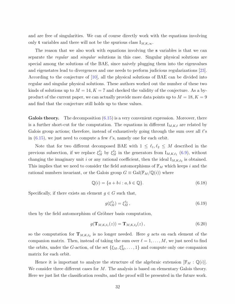
and are free of singularities. We can of course directly work with the equations involving

only t variables and there will not be the spurious class IM,K,∞.

The reason that we also work with equations involving the s variables is that we can

separate the regular and singular solutions in this case. Singular physical solutions are

special among the solutions of the BAE, since naively plugging them into the eigenvalues

and eigenstates lead to divergences and one needs to perform judicious regularizations [23].

According to the conjecture of [10], all the physical solutions of BAE can be divided into

regular and singular physical solutions. These authors worked out the number of these two

kinds of solutions up to M = 14, K = 7 and checked the validity of the conjecture. As a by-

product of the current paper, we can actually provide more data points up to M = 18, K = 9

and find that the conjecture still holds up to these values.

Galois theory. The decomposition (6.15) is a very convenient expression. Moreover, there

is a further short-cut for the computation. The equations in different IM,K,` are related by

Galois group actions; therefore, instead of exhaustively going through the sum over all `’s

in (6.15), we just need to compute a few `’s, namely one for each orbit.

Note that for two different decomposed BAE with 1 ≤ `1, `2 ≤ M described in the

previous subsection, if we replace ξ`1M by ξ`2M in the generators from IM,K,`1 (6.9), without

changing the imaginary unit i or any rational coefficient, then the ideal IM,K,`2 is obtained.

This implies that we need to consider the field automorphisms of FM which keeps i and the

rational numbers invariant, or the Galois group G ≡ Gal(FM/Q(i)) where

Q(i) = {a+ b i : a, b ∈ Q}. (6.18)

Specifically, if there exists an element g ∈ G such that,

g(ξ`1M) = ξ`2M , (6.19)

then by the field automorphism of Grobner basis computation,

g(TM,K,`1(z)) = TM,K,`2(z) , (6.20)

so the computation for TM,K,`2 is no longer needed. Here g acts on each element of the

companion matrix. Then, instead of taking the sum over ` = 1, . . . ,M , we just need to find

the orbits, under the G-action, of the set {ξM , ξ2M , . . . , 1} and compute only one companion

matrix for each orbit.

Hence it is important to analyze the structure of the algebraic extension [FM : Q(i)].

We consider three different cases for M . The analysis is based on elementary Galois theory.

Here we just list the classification results, and the proof will be presented in the future work.

32

1. M is odd. In this case, the field FM is the cyclotomic field,

FM = Q(ξM , i) = Q(ξ4M) = Q(e

2πi4M

). (6.21)

Note that i = ξM4M . The large Galois group, Gal(FM/Q), is the multiplication group

(Z/(4M)Z)× with the size φ(4M) = φ(4)φ(M) = 2φ(M). Here φ(. . .) is the Euler

totient function. We have

|G| = |Gal(FM/Q(i))| = φ(M) (6.22)

From elementary number theory, there exists a g ∈ G such that,

g(ξ`1M) = ξ`2M , g(i) = i . (6.23)

Hence IM,K,`1 and IM,K,`2 are equivalent if and only if gcd(`1,M) = gcd(`2,M). We

conclude that in this case, the ideals (6.9) are classified by the greatest common

divisors. Under the Galois group G, the number of orbits is σ0(M), where σ0(. . .)

denotes the divisor function which counts the number of divisors of M . Furthermore,

with the ideal IM,K,∞, we need to compute σ0(M) + 1 companion matrices when M is

odd.

2. M is even and 4 6 |M . In this case, the field FM is the cyclotomic field

FM = Q(ξM , i) = Q(ξ2M) = Q(e

2πi2M

). (6.24)

Gal(FM/Q) is the multiplication group (Z/(2M)Z)× with the size φ(2M) = φ(4)φ(M/2) =

2φ(M). We have

|Gal(FM/Q(i))| = φ(M). (6.25)

As in the previous case, IM,K,`1 and IM,K,`2 are equivalent if and only if gcd(`1,M) =

gcd(`2,M). We need to compute σ0(M) + 1 companion matrices, as in the preceding

case.

3. 4|M . This case is different from the previous ones. The field FM is the cyclotomic

field

FM = Q(ξM , i) = Q(ξM) = Q(e

2πiM

). (6.26)

Note that i is a power of ξM . G = Gal(FM/Q(i)) is the subgroup of Gal(FM/Q) which

keeps i invariant.

The classification of `’s is more complicated in this case, since i ∈ Q(ξM). From

detailed Galois theory analysis, IM,K,`1 and IM,K,`2 are equivalent if and only if

gcd(M, `1) = gcd(M, `2),`2`1

= 1 mod gcd

(M

gcd(M, `1), 4

). (6.27)

33

Note that the denominator of the reduced fraction `2/`1 is relatively prime toM/ gcd(M, `1),

so the congruence condition for `2/`1 is meaningful.

The condition (6.27) for 4|M is complicated. However, it is possible to simplify it

and get a similar condition as in the previous two cases. We notice that there is an

enhanced symmetry for the Q-system,

si 7→ (−1)k−isi, i = 0, . . . , K . (6.28)

Under this transformation, we find that up to M ≤ 16 the ideal IM,K is invariant.

Furthermore, the polynomial for the momentum condition transforms as

PM,K,`(i) 7→ (−1)KPM,K,`(−i) . (6.29)

This means that the imaginary unit i in PM,K,` transforms to −i. Hence, for two

integers `1 and `2, such that gcd(M, `1) = gcd(M, `2) but which do not satisfy (6.27),

when the enhanced symmetry (6.28) exists, IM,K,`1 and IM,K,`2 are still equivalent.

In summary, with the enhanced symmetry (6.28), for any positive integer M , IM,K,`1

and IM,K,`2 are equivalent if and only if gcd(M, `1) = gcd(M, `2). Hence there are always

σ0(M) + 1 classes.

6.3 Results on decomposition over FM

In this subsection, we give some results of BAE decomposition over the extended field FM .

M = 6

In this case F6 = Q(e

2πi12

). From the discussion of Galois theory in the previous section, the

decomposed BAE sub-systems are classified by the value of `:

{1, 5}, {2, 4}, {3}, {6}, {∞} . (6.30)

Two sub-systems, whose `-values live in the same class, are equivalent by a Galois group

action. Hence the number of solutions to the two sub-systems must be equal.

We compute the Grobner basis of I6,K,` with ` = 1, 2, 3, 4, 5, 6,∞, and get the Bethe root

counting for the decomposed BAE with M = 6 in Table 3. For the singular Bethe roots,

via the TQ-relation, we can find the values of their regularized momenta. These regularized

values are indicated by the numbers between brackets. For example, in Table 3, the entry

“0 (1)” for K = 2 and ` = 3 means that I6,2,3 has no solution but there is one singular

Bethe root whose regularized momentum value is e3×2πi/6 = eπi.

34

{1, 5} {2, 4} {3} {6} {∞}K = 1 1 1 1 0 0

K = 2 1 2 0 (1) 2 1

K = 3 1 0 2 0 (1) 1

Table 3: Number of Bethe roots for decomposed BAE with M = 6 . There are σ0(6) + 1 = 5

classes, which correspond to {1, 5}, {2, 4}, {3}, {6}, {∞}. The numbers in brackets are the

singular Bethe roots.

M = 7

In this case F7 = Q(e

2πi28

). The decomposed BAE sub-systems are classified by the value of

`:

{1, 2, 3, 4, 5, 6}, {7}, {∞} . (6.31)

Note that since 7 is a prime number, the classification of BAE sub-systems is very simple.

The root counting for the decomposed BAE with M = 7 is given in Table 4.

{1, 2, 3, 4, 5, 6} {7} {∞}K = 1 1 0 0

K = 2 2 2 0

K = 3 2 2 0

Table 4: Number of Bethe roots for decomposed BAE with M = 7.

M = 8

In this case F8 = Q(e

2πi8

). The decomposed BAE sub-systems are classified by the value of

`, via the condition (6.27):

{1, 5}, {2}, {3, 7}, {4}, {6}, {8}, {∞} . (6.32)

However, due to the enhanced symmetry (6.28), classes like {1, 5} and {3, 7} are equivalent,

and similarly {2} and {6} are also equivalent. Therefore we can use the new classification,

{1, 3, 5, 7}, {2, 6}, {4}, {8}, {∞} (6.33)

The root counting for the decomposed BAE with M = 8 is given in Table 5. Note that

for the cases M ≤ 8, each BAE subsystem contains at most four roots. Hence the Bethe

roots form a solvable algebraic extension over FM by Galois theory, which means that each

35

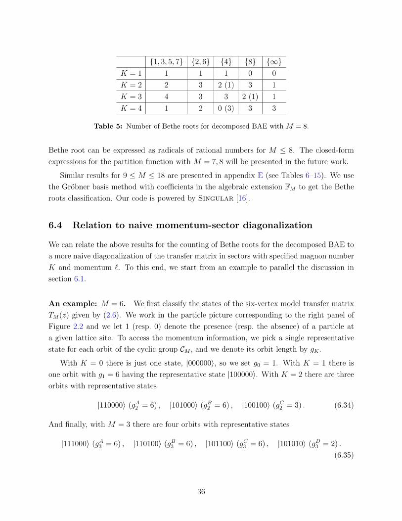
{1, 3, 5, 7} {2, 6} {4} {8} {∞}K = 1 1 1 1 0 0

K = 2 2 3 2 (1) 3 1

K = 3 4 3 3 2 (1) 1

K = 4 1 2 0 (3) 3 3

Table 5: Number of Bethe roots for decomposed BAE with M = 8.

Bethe root can be expressed as radicals of rational numbers for M ≤ 8. The closed-form

expressions for the partition function with M = 7, 8 will be presented in the future work.

Similar results for 9 ≤ M ≤ 18 are presented in appendix E (see Tables 6–15). We use

the Grobner basis method with coefficients in the algebraic extension FM to get the Bethe

roots classification. Our code is powered by Singular [16].

6.4 Relation to naive momentum-sector diagonalization

We can relate the above results for the counting of Bethe roots for the decomposed BAE to

a more naive diagonalization of the transfer matrix in sectors with specified magnon number

K and momentum `. To this end, we start from an example to parallel the discussion in

section 6.1.

An example: M = 6. We first classify the states of the six-vertex model transfer matrix

TM(z) given by (2.6). We work in the particle picture corresponding to the right panel of

Figure 2.2 and we let 1 (resp. 0) denote the presence (resp. the absence) of a particle at

a given lattice site. To access the momentum information, we pick a single representative

state for each orbit of the cyclic group CM , and we denote its orbit length by gK .

With K = 0 there is just one state, |000000〉, so we set g0 = 1. With K = 1 there is

one orbit with g1 = 6 having the representative state |100000〉. With K = 2 there are three

orbits with representative states

|110000〉 (gA2 = 6) , |101000〉 (gB2 = 6) , |100100〉 (gC2 = 3) . (6.34)

And finally, with M = 3 there are four orbits with representative states

|111000〉 (gA3 = 6) , |110100〉 (gB3 = 6) , |101100〉 (gC3 = 6) , |101010〉 (gD3 = 2) .

(6.35)

36

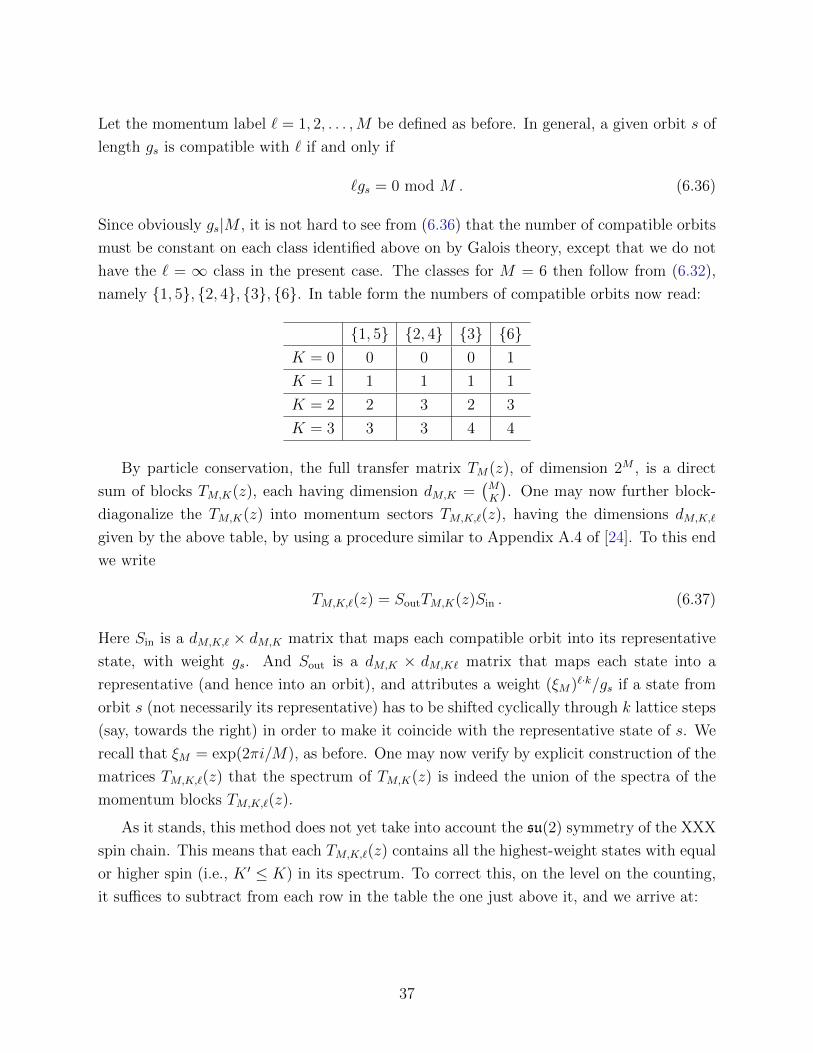
Let the momentum label ` = 1, 2, . . . ,M be defined as before. In general, a given orbit s of

length gs is compatible with ` if and only if

`gs = 0 mod M . (6.36)

Since obviously gs|M , it is not hard to see from (6.36) that the number of compatible orbits

must be constant on each class identified above on by Galois theory, except that we do not

have the ` = ∞ class in the present case. The classes for M = 6 then follow from (6.32),

namely {1, 5}, {2, 4}, {3}, {6}. In table form the numbers of compatible orbits now read:

{1, 5} {2, 4} {3} {6}K = 0 0 0 0 1

K = 1 1 1 1 1

K = 2 2 3 2 3

K = 3 3 3 4 4

By particle conservation, the full transfer matrix TM(z), of dimension 2M , is a direct

sum of blocks TM,K(z), each having dimension dM,K =(MK

). One may now further block-

diagonalize the TM,K(z) into momentum sectors TM,K,`(z), having the dimensions dM,K,`

given by the above table, by using a procedure similar to Appendix A.4 of [24]. To this end

we write

TM,K,`(z) = SoutTM,K(z)Sin . (6.37)

Here Sin is a dM,K,` × dM,K matrix that maps each compatible orbit into its representative

state, with weight gs. And Sout is a dM,K × dM,K` matrix that maps each state into a

representative (and hence into an orbit), and attributes a weight (ξM)`·k/gs if a state from

orbit s (not necessarily its representative) has to be shifted cyclically through k lattice steps

(say, towards the right) in order to make it coincide with the representative state of s. We

recall that ξM = exp(2πi/M), as before. One may now verify by explicit construction of the

matrices TM,K,`(z) that the spectrum of TM,K(z) is indeed the union of the spectra of the

momentum blocks TM,K,`(z).

As it stands, this method does not yet take into account the su(2) symmetry of the XXX

spin chain. This means that each TM,K,`(z) contains all the highest-weight states with equal

or higher spin (i.e., K ′ ≤ K) in its spectrum. To correct this, on the level on the counting,

it suffices to subtract from each row in the table the one just above it, and we arrive at:

37

{1, 5} {2, 4} {3} {6}K = 0 0 0 0 1

K = 1 1 1 1 0

K = 2 1 2 1 2

K = 3 1 0 2 1

This can finally be compared with Table 3. It is seen that the two tables are identical, in so

far as they assign the same dimensions to the same (K, `) sectors. Notice that the present

approach does not particularize the singular case denoted {∞} in Table 3, but assigns to

it straight away the correct regularized momentum, namely {∞} → {3} for K = 2, and

{∞} → {6} for K = 3.3 The counting is consistent with the sum of numbers outside and

inside the brackets in Table 3.

General case. The case of general M can be treated in the same way. To recover the

results corresponding to Tables 3–15, we only need to know the number of compatible

orbits under CM for each set of (K, `). In even simpler terms, pick a divisor gs|M , and let

N(gs;M,K) be the number of orbits of length gs with K magnons. For instance, we have

N(gs; 6, 2) = 0, 0, 1, 2 and N(gs; 6, 3) = 0, 1, 0, 3 for gs = 1, 2, 3, 6, respectively. From this

data, the dimensions dM,K,` is the sum over those N(gs;M,K) that respect the criterion

(6.36), and the highest-weight combinations dM,K,`−dM,K−1,` provide precisely the numbers

of Tables 3–15, up to the assignment of a definite momentum to the {∞} classes.

We have written a simple algorithm that carries out this computation. It produces the

tables for M ≤ 24 in less than one minute. For M ≤ 18 these are in full agreement with

Tables 3–15, after assigning to each {∞} case the corresponding regularized momentum.

We note that for M even, this assignment appears to obey a simple rule: {∞} → {M/2}when K is even, and {∞} → {M} when K is odd. When M is prime, the decomposition

of the BAE is very simple, and there is no {∞}. It remains to discuss the cases of odd non-

prime M ≤ 18, namely M = 9 and M = 15. For M = 9 we find that {∞} → {3, 6} when

K = 3 (see Table 6), and for M = 15 we have {∞} → {5, 10} when K = 3 (see Table 12).

But we do not presently know how to establish such assignments for general M,K, without

going through the actual computations of regularization via the TQ-relations.

To summarize, the computations described in this subsection appear to be an efficient

short-cut for obtaining the decomposition dimension counting of Tables 3–15, without ever

actually using the integrability of the XXX chain, analysing the BAE, or doing any algebraic

geometry. This suggests that the solutions of the BAE simply decompose in a way that

3The first of these identifications agrees as well with Table 2 for the subspace called A there.

38

respects the conservation of spin and momentum, and the su(2) symmetry of the XXX

chain, with no extra hidden structure. But obviously the decomposition of the BAE goes

much further than the mere counting of dimensions; in particular the explicit results for

the Grobner bases make possible the efficient computations of the partition functions, as

we have seen.

7 Conclusions and discussions

In this paper we developed a method to compute the torus partition function of the six-

vertex model exactly and analytically. The method is based on an algebro-geometrical

approach to the BAE, together with new ingredients that include the rational Q-system,

primary decomposition, algbraic extension and Galois theory.

Using this approach, we probed new structures in the solution space of the BAE. We

found that the solution space can be decomposed into subspaces IM,K,` on an algebraically

extended field FM = Q(i, ξM), where M,K are the length, magnon number, and ` =

1, · · · ,M is related to the total momentum 2π`/M of the solutions of the BAE. We classified

the subspaces that are related by the action of the Galois group and form an orbit. For

each orbit, we computed the Grobner basis, quotient ring and the companion matrices of

the transfer matrix TM,K,`(z) and Baxter’s Q-operator QM,K,`(z) up to M = 14. This

decomposition can also be understood in terms of a naive momentum-sector decomposition

described in section 6.4. The decomposition of the solution space into IM,K,` and the use of

Galois theory led to a huge boost in the computation of the partition function. For M ≤ 6,

we have closed-form expressions for the partition function for any N . For larger M up to

M = 14, the partition functions for fixed N can be computed straightforwardly from the

companion matrices TM,K,`(z).

The exact partition functions are polynomials in the spectral parameter z of order MN

with rational coefficients. When M and N become large, we obtain polynomials with high

orders and large coefficients. Since polynomials are essentially specified by their zeros, we

solved for the zeros of the partition functions numerically to high accuracy and studied

their behavior in the partial thermodynamic limit where N � M and M is fixed. We

observed that the zeros accumulate on some curves in this limit and gave a numerical

method to generate the limiting curves of accumulation points. These curves exhibit some

universal behaviors for different values of even and odd M which led us to formulate several

observations and conjectures.

There are many open questions and new directions that one can pursue in the near

39

future. We discuss some of them in what follows.

An immediate interesting direction is to generalize the current work to the the quantum

deformed case. In this paper, we focussed on the six-vertex model at the isotropic point

where the model is equivalent to the Heisenberg XXX spin chain. Away from the isotropic

point, the six-vertex model is still integrable and is equivalent to the XXZ spin chain. In the

XXZ spin chain, we have a new parameter q which is related to the anisotropy. The isotropic

point corresponds to q = 1. Usually the BAE of the XXZ spin chain are written in terms

of hyperbolic or trigonometric functions, and one might wonder how our approach, which

seems to be restricted to rational functions, can be applied to this case. It is actually quite

simple to perform a change of variables to recast the BAE in terms of rational functions.

To study the solution space of the BAE and the torus partition function as in this paper,

we will however have to deal with several very interesting new features.

• First of all, one needs to distinguish between the cases where q takes a generic complex

value and the cases where q is a root of unity. It is well known that the latter case is

much more subtle than the former, in terms of solutions of BAE. The completeness

problem for the generic q case is a straightforward generalization of the XXX case,

namely the physical solutions consist of regular and physical singular solutions [25].

On the other hand, when q is a root of unity, due to the presence of the so-called

exact K-strings, there are seemingly infinitely many solutions and the situation for

the completeness problem is less clear. It is therefore not clear what are the physical

solutions. Before we can compute the torus partition function, it seems that we need

to sort out clearly the completeness problem first, which is an interesting question in

its own right. Some preliminary calculations show that algebro-geometric methods in

these cases are again very useful. For example, we observe that the Grobner bases

exhibit singularities when q is a root of unity and the quotient rings become affine

varieties with positive dimensions (instead of a collection of points).

• The six-vertex model is closely related to another famous model, namely the Potts

model. The latter can be represented in terms of the affine Temperley-Lieb (TL)

algebra (see, e.g., [24, 26] for a recent overview). The dimensions NM,K given in (3.6)

appear naturally as the dimension of standard modules of the affine TL algebra, which

we denote by Wj,z (for the isotropic case, we take z = 1). The representations of the

affine TL algebra take the graphical form of “link patterns” with pairwise connections

(arcs) and defect lines (through-lines) where the total number of lines and the number

of defect lines j play the role of length M and magnon number K, respectively, in our

40

context. To compute the torus partition function of such models,4 one can perform

a decomposition within the standard module with respect to the lattice momentum

[24], which is essentially the same as what we did in section 6.4. Let us recall that

in our case the decomposition comes completely from studying the solution space of

the BAE (or the rational Q-system) using algebraic geometry and the dimensions of

the subspaces come from counting the number of solutions; while in the Potts model

case, these come from studying the representation theory of the affine TL algebra.

These similarities are quite remarkable and imply that the physical solutions of the

BAE, studied here using the algebro-geometric approach, actually know a lot about

the representation theory of affine TL algebra. It will be interesting to see to which

extent these connections carry over to the q-deformed case.

• For generic q, we need to consider the standard moduleWj,z with non-trivial z, namely

z 6= 1. In this case, there is another quantum number that appears which is associated

with z. This is related to the momentum with which the defects spiral around the

periodic direction. It will be intriguing to see how such a new quantum number can

appear in our context by studying the solutions space of the BAE.

• The case when q is a root of unity is even more interesting. In that case, representations

of affine TL should be reducible, but indecomposable. In practice, this will mean

that the Wj,z will have to be “glued” in various ways [27, 28]. The complexity of

these gluings and the expected appearance of Jordan cells will challenge the algebro-

geometric approach. It will be very exciting to see how these structures carry over to

the solution space of the BAE.

In the current work, we considered periodic boundary condition in both directions for

the lattice. This corresponds to the torus partition function. It is also interesting to consider

the partition function on other topologies, such as an annulus [6]. For this topology, we

need to compute the transfer matrix of the spin chain with open boundary conditions. One

nice starting point for this case is the quantum group invariant XXZ spin chain [29]. This

spin chain is invariant under the quantum group Uq(sl(2)). It has several nice properties.

In particular, the completeness problem has been studied systematically in [30] both for

generic q, and q at roots of unity. The relation with TL algebra has also been established.

Working out this simpler example should also shed light on the more challenging periodic

boundary conditions mentioned above.

4Notice that these have previously been studied by more combinatorial methods in the special case of

the chromatic polynomial [7].

41

For the zeros of partition function, it will be desirable to find an analytic approach to

understand or even predict the condensation curves in the partial thermodynamic limit.

It is also interesting to see how the q-deformation affects the distribution of the partition

function zeros.

Acknowledgements

Y. Jiang is partially supported by the Swiss National Science Foundation through the

NCCR SwissMap. J.L. Jacobsen acknowledges support from the European Research Council

through the advanced grant NuQFT. Y. Zhang is supported by funding from Swiss National

Science Foundation (Ambizione grant PZ00P2 161341) and the European Research Council

(ERC) under the European Union’s Horizon 2020 research and innovation programme (grant

agreement No 725110). We thank Zoltan Bajnok, Janko Bohm, Matthias Staudacher and

Yuwei Zhang for helpful discussions.

A Rational Q-system

In this appendix, we review the rational Q-system method for solving Bethe ansatz equations

(BAE) proposed by Marboe and Volin [11]. One of the main advantages of this method is

that unlike the BAE, the solutions of the rational Q-system are all physical. In addition,

it is by far the most efficient way of finding Bethe roots for fixed length M and particle

number K.

Let us briefly review how the rational Q-system works. For more details, we refer to

the original papers [11, 12]. The method works for a large class of rational spin chains with

su(m,n|k) symmetry. For our purpose, we restrict to the su(2) case. The main procedure

is as follows:

1. For a BAE of length M and magnon number K, we draw a Young diagram of two

rows (M −K,K) with M −K ≤ K. 5

2. To each node (i.e., a corner of a box of the Young diagram) we associate a Q-

function and require that all the Q-functions are polynomials. The order of a given

Q-polynomial is given by the number of boxes on the upper-right part of the corre-

sponding node (see figure A.8 for an illustration).

5Since the solution of BAE gives the same eigenstate as the corresponding dual solution, this restriction

already covers the whole Hilbert space.

42

3. Some of the Q-functions at the boundary are completely fixed and do not need to be

solved. The Q-functions at the upper right boundary are completely fixed to be 1

since there are no Bethe roots. In addition, the Q-polynomial at node (0, 0) is given

by uM .

4. The rest of the Q-functions are determined by the QQ-relations

Qa+1,s(u)Qa,s+1(u) = Q+a+1,s+1(u)Q−a,s(u)−Q−a+1,s+1(u)Q+

a,s(u) , (A.1)

where Qa,s denotes the Q-function associated with the node at position (a, s). The

QQ-relation (A.1) is a relation between the four nodes around a box. Here and in

what follows, we introduce the shorthand notations

Q±a,s(u) = Qa,s(u± i/2), Q++a,s (u) = Qa,s(u+ i), Q−−a,s (u) = Qa,s(u− i). (A.2)

To determine these polynomials, one makes an ansatz for the unknown Q-polynomials

along certain path (see the example in the next subsection) and require that all the

Q-functions on the Young tableaux are polynomials. This leads to a set of algebraic

equations for the unknown coefficients. Solving this set of algebraic equations gives

the Q-polynomials.

5. The Bethe roots of length M and magnon number K are given by the zeros of Q0,1(u).

This fact will be shown below.

In order to explain the above procedure, we give an explicit example in the next subsection.

A.1 A simple example

In order to explain the method, we consider a simple example with M = 6 and K = 2, where

M is the length of the spin chain and K is the number of magnons. The corresponding

Young diagram is given by (M −K,K) = (4, 2), and is shown in figure A.8. The number

on each node denotes the degree of the corresponding Q-polynomial. There are thirteen

Q-functions on the Young tableaux, each Q-polynomial being associated with a node of the

Young tableaux. The boundary nodes (the ones labeled by 0) are simply taken to be 1. In

addition, the Q-polynomial at the origin is taken to be

Q0,0(u) = u6. (A.3)

One needs to choose a path from the origin to the upper right boundary. We have chosen

the one with yellow color in figure A.8. Apart from the two boundary Q-polynomials, there

43

Figure A.8: The Young diagram for M = 6, K = 2. The number on each node denotes the

degree of the Q-polynomial.

are two other unknown Q-polynomials which are parameterized by

Q0,1(u) = u2 + c(1)0,1 u+ c

(0)0,1, Q1,1 = u+ c

(0)1,1. (A.4)

The remaining task is to use the QQ-relations (A.1) to determine the remaining unknown

Q-polynomials as well as the coefficients c(1)0,1, c

(0)0,1 and c

(0)1,1. In fact, in our case there are only

three remaining non-trivial functions to be determined, namely Q1,0,Q2,0 and Q3,0.

Let us first determine Q1,0(u). Taking a = s = 0, the QQ-relation leads to

Q1,0(u) = cQ+

1,1(u)Q−0,0(u)−Q−1,1(u)Q+0,0(u)

Q0,1(u)(A.5)

where c is some normalization constant to make the polynomial monic. The quotient and

the remainder can be computed straightforwardly. Plugging (A.3) and (A.4) into (A.5), we

find a non-trivial remainder in terms of the unknown coefficients c(1)0,1, c

(0)0,1 and c

(0)1,1. Since

by definition Q1,0(u) is a polynomial, the remainder should be zero. This leads to a set of

equations for the unknown coefficients. These relations are called zero remainder conditions

(ZRC). Repeating this analysis for all the other non-trivial Q-functions, we obtain the full

set of ZRC, which are the systems of equations that we need to solve.

The paths can be chosen in different ways, which result in different forms of ZRC, but

finally they lead to the same solution of rational Q-systems. The simplest choice of the path

is the one that goes from (0, 0) to (0, 2) and then from (0, 2) to the rightmost node (K, 2).

In this way, we only have one unknown Q-function, namely Q0,1, to determine.

After solving the ZRC, we find all the Q-polynomials. The Bethe roots are simply given

by the zeros of Q0,1(u). This is proved in the next subsection.

44

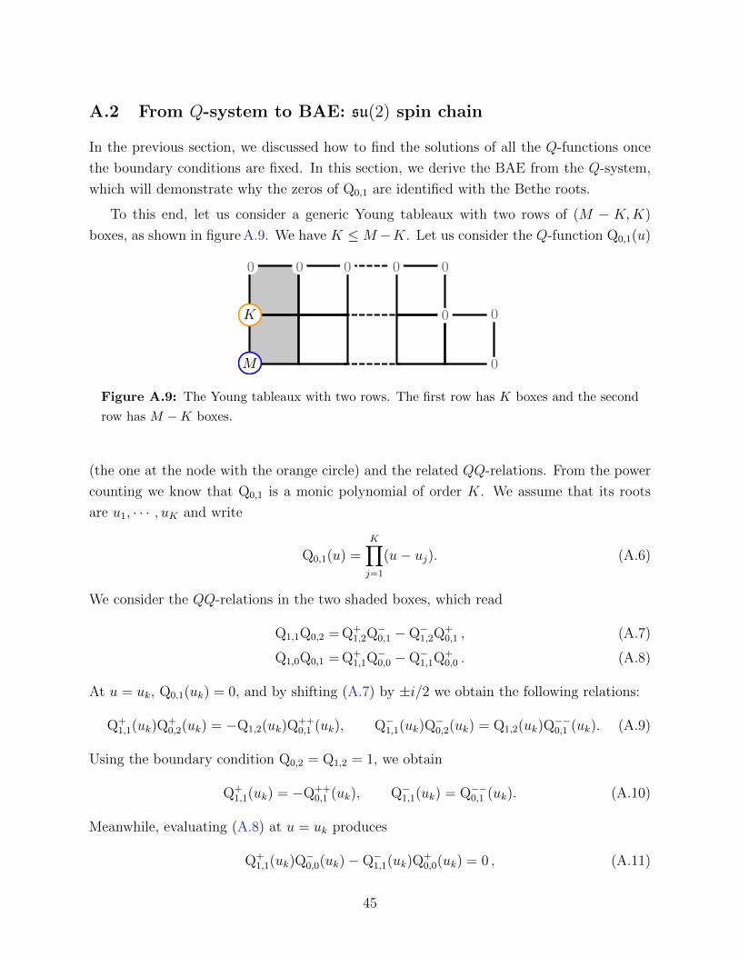
A.2 From Q-system to BAE: su(2) spin chain

In the previous section, we discussed how to find the solutions of all the Q-functions once

the boundary conditions are fixed. In this section, we derive the BAE from the Q-system,

which will demonstrate why the zeros of Q0,1 are identified with the Bethe roots.

To this end, let us consider a generic Young tableaux with two rows of (M − K,K)

boxes, as shown in figure A.9. We have K ≤M−K. Let us consider the Q-function Q0,1(u)

Figure A.9: The Young tableaux with two rows. The first row has K boxes and the second

row has M −K boxes.

(the one at the node with the orange circle) and the related QQ-relations. From the power

counting we know that Q0,1 is a monic polynomial of order K. We assume that its roots

are u1, · · · , uK and write

Q0,1(u) =K∏j=1

(u− uj). (A.6)

We consider the QQ-relations in the two shaded boxes, which read

Q1,1Q0,2 = Q+1,2Q

−0,1 −Q−1,2Q

+0,1 , (A.7)

Q1,0Q0,1 = Q+1,1Q

−0,0 −Q−1,1Q

+0,0 . (A.8)

At u = uk, Q0,1(uk) = 0, and by shifting (A.7) by ±i/2 we obtain the following relations:

Q+1,1(uk)Q

+0,2(uk) = −Q1,2(uk)Q

++0,1 (uk), Q−1,1(uk)Q

−0,2(uk) = Q1,2(uk)Q

−−0,1 (uk). (A.9)

Using the boundary condition Q0,2 = Q1,2 = 1, we obtain

Q+1,1(uk) = −Q++

0,1 (uk), Q−1,1(uk) = Q−−0,1 (uk). (A.10)

Meanwhile, evaluating (A.8) at u = uk produces

Q+1,1(uk)Q

−0,0(uk)−Q−1,1(uk)Q

+0,0(uk) = 0 , (A.11)

45

and plugging (A.10) into (A.11) we obtain

Q++0,1 (uk)Q

−0,0(uk) + Q−−0,1 (uk)Q

+0,0(uk) = 0. (A.12)

Use the boundary condition and the expression for Q0,1(u),

Q0,0(u) = uM , Q0,1(u) =K∏j=1

(u− uj) , (A.13)

we finally arrive at (uk + i/2

uk − i/2

)M= −

K∏j=1

uk − uj + i

uj − uk − i, (A.14)

which is nothing but the BAE of SU(2) spin chain with length M and magnon number K.

It follows in particular that the roots uj of Q0,1(u) are precisely the Bethe roots, so we can

identify the latter with the Baxter polynomial (2.14), viz. Q0,1(u) = Q(u), as previously

claimed.

B More on algebraic geometry

In this appendix, we briefly review the important algebraic geometry technique used in

our paper, primary decomposition. The mathematics reference is [31]. For the concept of

Grobner basis and companion matrix, we refer to the introduction in [2].

Let F be a field and A = F[z1, . . . zn] be a polynomial. Any ideal I in A decomposes into

the intersection of several primary ideals.

I = I1 ∩ I2 ∩ . . . ∩ Ik , (B.1)

where each Ij is primary. A primary ideal J is an ideal such that if a, b ∈ A, ab ∈ J , then

either a ∈ J or bn ∈ J . The decomposition (B.1) is an analogy for the factorization of

integers.

Note that with the decomposition (B.1), geometrically, the zero sets of I decompose into

the union of several algebraic sets

Z(I) = Z(I1) ∪ Z(I2) ∪ . . . ∪ Z(Ik) . (B.2)

This property is useful for the study of the complicated zero set Z(I). Especially, when

Z(I) is zero-dimensional, like the set of Bethe roots, this decomposition classifies the Bethe

roots and we shall call each Ij decomposed BAE.

46

Note that the definition of primary decomposition depends on the coefficient field F. For

example, within Q[x, y],

〈x2 − 2y2〉 (B.3)

is already primary and hence cannot be decomposed further. However, within the algebraic

closure Q[x, y], we have the primary decomposition:

〈x2 − 2y2〉 = 〈x− y√

2〉 ∩ 〈x+ y√

2 〉 . (B.4)

We refer to [31] for the introduction of algebraic extension and Galois theory. The

computation of primary decomposition can be carried out by the computer algebra system

Singular [16].

C Power of companion matrices

The main method we present in this paper to compute partition function is to calculate

the companion matrices for BAE. Recall that, according to (3.14), the six-vertex model

partition function is given by

ZM,N =

[M/2]∑K=0

(M − 2K + 1) Tr(TM,K(z)N

), (C.1)

where TM,K(z) is the companion matrix of the polynomial tM,K(s, z). Recall also that

TM,K(z), calculated from the Grobner basis, contains only rational numbers. Therefore the

whole computation is manifestly analytic.

In practice, although TM,K(z) can be calculated from the straightforward Grobner

basis and polynomial division procedure, the matrix power TM,K(z)N computation can

be difficult.

We here present an alternative algorithm which speeds up the computation and saves

RAM usage. The algorithm can be sketched as follows:

1. For given M and K, calculate the Grobner basis G(IM,K).

2. Divide tM,K(s, z) towards G(IM,K); the remainder tM,K(s, z) is called the normal form.

3. AssumeN is a power of 2, i.e., N = 2c. Recursively compute t(i)M,K(s, z) ≡ (t

(i−1)M,K (s, z))2,

for i = 2, . . . , c+ 1, where t(1)M,K(s, z) ≡ tM,K(s, z). Divide t

(i)M,K(s, z) towards G(IM,K)

and define t(i)M,K(s, z) to be the remainder.

47

4. Calculate the companion matrix of t(c+1)M,K (s, z). This is the demanded companion

matrix TM,K(z)N .

This strategy avoids the storage and multiplication of dense matrices. Here we used

the algebraic geometry property (3.9) that the companion matrix of a product of two

polynomials, equals the product of the corresponding two companion matrices. If N is

not a power of 2, we find the binary representation of N which is N = 2c1 + 2c2 + ... and

repeat the computation several times.

In this algorithm, we trim each intermediate polynomial t(i)M,K(s, z) towards G(IM,K) via

the polynomial division, to get a much short polynomial t(i)M,K(s, z). This significantly saves

the RAM usage.

This algorithm can also be combined with the decomposition described in Section 6. In-

stead of calculating G(IM,K), we calculate G(IM,K,`) over the algebraic extension FM . Since

Z(IM,K,`) contains much fewer points than those inZ(IM,K), the quotient ring FM [s0, . . . sK−1]/IM,K,`

has much lower dimension. Hence the polynomial division step trims the polynomial size

more dramatically and further speeds up the computation. By (6.20), we just need to

compute σ0(M) + 1 distinct TM,K,l(z)N , and get the rest by the Galois group action.

Our algorithm is powered by the Singular [16] code. For the application with decom-

posed BAE, we introduce ξM through the minpoly command in Singular with the explicit

minimal polynomial for ξM (cyclotomic polynomial).

D Details on finding limiting curves

We here describe the numerical procedure employed in Section 5.2 to find the limiting curves

along which the partition function zeros ZM,N(z) = 0 accumulate, in the limit N →∞, for

a fixed value of M .

The key ingredient is obviously to be able to efficiently diagonalize the transfer matrix,

so that the loci of equimodularity (|Λ1(z)| = |Λ2(z)|) can be identified. To this end, we do

not need the entire spectrum of TM(z) but only the first few eigenvalues (in principle, just

the first two, but see the remarks below). The most efficient means of finding those are

iterative Krylov-subspace methods that depend only on implementing the multiplication

of the transfer matrix with a vector, i.e., to compute v′ = TM(z)v when given some

vector v. Our method of choice is the Arnoldi algorithm, for which we use the Arpack

implementation of Arnoldi’s algorithm for complex matrices [32].6 This implementation is

6We thank C.R. Scullard for technical discussions about the use of Arpack.

48

capable of sorting the eigenvalues in order of decreasing norm.

A huge advantage of such iterative methods is that TM(z) is given as a product of sparse

matrices via (2.6), where each R-matrix contains at most two non-zero entries per column.

Therefore the computation of v′ in each iteration requires at most 2Md operations, where

d is the dimension of the matrix. The trace Tr a is performed by going from M to M + 2

sites when the auxiliary space is inserted, and back to M sites after a row of the lattice has

been completed and the trace operation performed.

If the magnon and momentum labels (K, `) for the equimodular eigenvalues Λ1(z) and

Λ2(z) were known beforehand, it would obviously be most efficient to diagonalize the smaller

matrices TM,K,`(z) constructed in (6.37). But since the accumulation curves in practice

turn out to have multiple branches and T-points where the sector labels may change, this

approach would necessitate a considerable amount of manual intervention. We have thus

chosen a more brute-force approach in which the entire matrix TM(z) is diagonalized, for

all K = 0, 1, . . . , bM/2c simultaneously and with decomposing the momentum with respect

to the ` label. Note that the su(2) highest-weight constraint is also not enforced in this

approach, so the eigenvalues with K < bM/2c present degeneracies. We deal with this

in practice by imposing the equimodularity criterion |Λ1(z)| = |Λr(z)|, where r ≥ 2 is a

suitably chosen (small) integer, which may need some adjustment as we run through the

various branches of the equimodular curves.

The first step in our procedure is to acquire some approximate knowledge about where

to start the search for the equimodular curves. In the case of Figure 5.5 we first made a

rough plot of the norms of the first few eigenvalues along a few straight lines with constant

Re z, or along the real axis, to get a finite list of points close to the equimodular curves. In

a second step, we then launched a direct-search algorithm, taking each of these points as

the initial point. The direct-search method is carefully described in [3]; it has the property

of first locking onto any close-by equimodular curve and then following it in small steps.7

The search is stopped whenever a branch of the equimodular wanders off to infinity, or if it

starts overlapping with a part of the curve which is already known. One all starting points

have been exploited, we have completed the second step.

The third and final step consists in making sure that the set of equimodular curves is

complete. This requires in particular examining carefully the surroundings of any point

where the curves present a discontinuous tangent vector, since this is the sign of a T-point

or a higher-order bifurcation point. As in the first step, we make a rough plot of the norms

along a small circle surrounding any potential bifurcation point. If a branch is identified

7We chose |∆z| = 10−2 in most cases, but decreased to 10−3 close to T-points and other fine details.

49

that has not yet been traced out, we go back to the second step as many times as necessary.

Obviously, if the whole set of equimodular curves has some very small disconnected

pieces, they may be missed by this procedure. However, the fact that the curves in Figure 5.5

present only a single connected component gives appealing evidence that they are actually

complete.

50

E More results of primary decomposition on FM

In this appendix, we list the results of primary decomposition on FM for 9 ≤M ≤ 18.

{1, 2, 4, 5, 7, 8} {3, 6} {9} {∞}K = 1 1 1 0 0

K = 2 3 3 3 0

K = 3 5 5 (1) 6 2

K = 4 5 4 4 0

Table 6: Number of Bethe roots for decomposed BAE with M = 9.

{1, 3, 7, 9} {2, 4, 6, 8} {5} {10} {∞}K = 1 1 1 1 0 0

K = 2 3 4 2 (1) 4 1

K = 3 8 7 8 6 (1) 1

K = 4 8 10 4 (4) 10 4

K = 5 5 3 6 0 (4) 4

Table 7: Number of Bethe roots for decomposed BAE with M = 10.

{1, 2, 3, 4, 5, 6, 7, 8, 9, 10} {11} {∞}K = 1 1 0 0

K = 2 4 4 0

K = 3 10 10 0

K = 4 15 15 0

K = 5 12 12 0

Table 8: Number of Bethe roots for decomposed BAE with M = 11.

51

{1, 5, 7, 11} {2, 10} {3, 9} {4, 8} {6} {12} {∞}K = 1 1 1 1 1 1 0 0

K = 2 4 5 4 5 4 (1) 5 1

K = 3 13 12 14 12 13 12 (1) 1

K = 4 22 24 21 25 18 (5) 24 5

K = 5 26 24 26 23 24 18 (5) 5

K = 6 9 12 10 12 4 (10) 14 10

Table 9: Number of Bethe roots for decomposed BAE with M = 12.

{1, 2, 3, 4, 5, 6, 7, 8, 9, 10, 11, 12} {13} {∞}K = 1 1 0 0

K = 2 5 5 0

K = 3 16 16 0

K = 4 33 33 0

K = 5 44 44 0

K = 6 33 33 0

Table 10: Number of Bethe roots for decomposed BAE with M = 13.

{1, 3, 5, 9, 11, 13} {2, 4, 6, 8, 10, 12} {7} {14} {∞}K = 1 1 1 1 0 0

K = 2 5 6 4 (1) 6 1

K = 3 20 19 20 18 (1) 1

K = 4 44 47 38 (6) 47 6

K = 5 73 70 73 64 (6) 6

K = 6 69 74 54 (15) 74 15

K = 7 33 28 34 14 (15) 15

Table 11: Number of Bethe roots for decomposed BAE with M = 14.

52

{1, 2, 4, 7, 8, 11, 13, 14} {3, 6, 9, 12} {5, 10} {15} {∞}K = 1 1 1 1 0 0

K = 2 6 6 6 6 0

K = 3 23 24 22 (1) 24 2

K = 4 61 60 61 60 0

K = 5 109 109 110 110 0

K = 6 133 135 132 134 0

K = 7 96 94 96 94 0

Table 12: Number of Bethe roots for decomposed BAE with M = 15.

{1, 3, 5, 7, 9, 11, 13, 15} {2, 6, 10, 14} {4, 12} {8} {16} {∞}K = 1 1 1 1 1 0 0

K = 2 6 7 7 6 (1) 7 1

K = 3 28 27 27 27 26 (1) 1

K = 4 77 80 81 74 (7) 81 7

K = 5 161 158 157 157 150 (7) 7

K = 6 224 231 231 210 (21) 231 21

K = 7 218 211 211 211 190 (21) 21

K = 8 85 93 94 60 (35) 95 35

Table 13: Number of Bethe roots for decomposed BAE with M = 16.

{1, 2, 3, 4, 5, 6, 7, 8, 9, 10, 11, 12, 13, 14, 15, 16} {17} {∞}K = 1 1 0 0

K = 2 7 7 0

K = 3 32 32 0

K = 4 100 100 0

K = 5 224 224 0

K = 6 364 364 0

K = 7 416 416 0

K = 8 286 286 0

Table 14: Number of Bethe roots for decomposed BAE with M = 17.

53

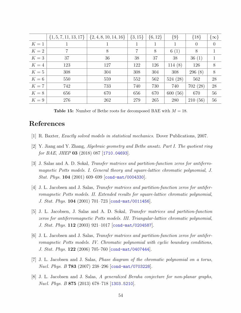
{1, 5, 7, 11, 13, 17} {2, 4, 8, 10, 14, 16} {3, 15} {6, 12} {9} {18} {∞}K = 1 1 1 1 1 1 0 0

K = 2 7 8 7 8 6 (1) 8 1

K = 3 37 36 38 37 38 36 (1) 1

K = 4 123 127 122 126 114 (8) 126 8

K = 5 308 304 308 304 308 296 (8) 8

K = 6 550 559 552 562 524 (28) 562 28

K = 7 742 733 740 730 740 702 (28) 28

K = 8 656 670 656 670 600 (56) 670 56

K = 9 276 262 279 265 280 210 (56) 56

Table 15: Number of Bethe roots for decomposed BAE with M = 18.

References

[1] R. Baxter, Exactly solved models in statistical mechanics. Dover Publications, 2007.

[2] Y. Jiang and Y. Zhang, Algebraic geometry and Bethe ansatz. Part I. The quotient ring

for BAE, JHEP 03 (2018) 087 [1710.04693].

[3] J. Salas and A. D. Sokal, Transfer matrices and partition-function zeros for antiferro-

magnetic Potts models. I. General theory and square-lattice chromatic polynomial, J.

Stat. Phys. 104 (2001) 609–699 [cond-mat/0004330].

[4] J. L. Jacobsen and J. Salas, Transfer matrices and partition-function zeros for antifer-

romagnetic Potts models. II. Extended results for square-lattice chromatic polynomial,

J. Stat. Phys. 104 (2001) 701–723 [cond-mat/0011456].

[5] J. L. Jacobsen, J. Salas and A. D. Sokal, Transfer matrices and partition-function

zeros for antiferromagnetic Potts models. III. Triangular-lattice chromatic polynomial,

J. Stat. Phys. 112 (2003) 921–1017 [cond-mat/0204587].

[6] J. L. Jacobsen and J. Salas, Transfer matrices and partition-function zeros for antifer-

romagnetic Potts models. IV. Chromatic polynomial with cyclic boundary conditions,

J. Stat. Phys. 122 (2006) 705–760 [cond-mat/0407444].

[7] J. L. Jacobsen and J. Salas, Phase diagram of the chromatic polynomial on a torus,

Nucl. Phys. B 783 (2007) 238–296 [cond-mat/0703228].

[8] J. L. Jacobsen and J. Salas, A generalized Beraha conjecture for non-planar graphs,

Nucl. Phys. B 875 (2013) 678–718 [1303.5210].

54

[9] J. L. Jacobsen, J. Salas and C. R. Scullard, Phase diagram of the triangular-lattice

Potts antiferromagnet, J. Phys. A: Math. Theor. 50 (2017) 345002 [1702.02006].

[10] W. Hao, R. I. Nepomechie and A. J. Sommese, Completeness of solutions of Bethe’s

equations, Phys. Rev. E 88 (2013), no. 5 052113 [1308.4645].

[11] C. Marboe and D. Volin, Fast analytic solver of rational Bethe equations, J. Phys. A50

(2017), no. 20 204002 [1608.06504].

[12] C. Marboe and D. Volin, The full spectrum of AdS5/CFT4 I: Representation theory

and one-loop Q-system, 1701.03704.

[13] D. A. Cox, J. Little and D. O’Shea, Ideals, varieties, and algorithms. Undergraduate

Texts in Mathematics. Springer, Cham, fourth ed., 2015. An introduction to

computational algebraic geometry and commutative algebra.

[14] J.-C. Faugere, A new efficient algorithm for computing Grobner bases (F4), J. Pure

Appl. Alg. 139 (1999) 61–88.

[15] J. C. Faugere, A new efficient algorithm for computing Grobner bases without reduction

to zero (F5), in Proceedings of the 2002 International Symposium on Symbolic and

Algebraic Computation, ISSAC ’02, (New York, NY, USA), pp. 75–83, ACM, 2002.

[16] W. Decker, G.-M. Greuel, G. Pfister and H. Schonemann, “Singular 4-1-1 —

A computer algebra system for polynomial computations.” http://www.singular.

uni-kl.de, 2018.

[17] C. N. Yang and T. D. Lee, Statistical theory of equations of state and phase transitions.

I. Theory of condensation, Phys. Rev. 87 (Aug, 1952) 404–409.

[18] M. Fisher, The nature of critical points, in Lecture notes in theoretical physics

(W. Brittin, ed.), vol. 7c, (Boulder), pp. 1–159, University of Colorado Press, 1965.

[19] S. Beraha, J. Kahane and N. J. Weiss, Limits of zeroes of recursively defined

polynomials, Proc. Natl. Acad. Sci. 72 (1975) 4209–4209.

[20] D. A. Bini and L. Robol, Solving secular and polynomial equations: A multiprecision

algorithm, J. Comp. Appl. Math. 272 (2015) 276–292.

[21] O. Aberth, Iteration methods for finding all zeros of a polynomial simultaneously, Math.

Comp. 27 (1973) 339–344.

55

[22] Y. Jiang and Y. Zhang, Algebraic Geometry and Bethe Ansatz. Part II. Primary

decomposition and algebraic extensions., to appear.

[23] R. I. Nepomechie and C. Wang, Algebraic Bethe ansatz for singular solutions, J. Phys.

A 46 (2013) 325002 [1304.7978].

[24] J. L. Jacobsen and H. Saleur, Bootstrap approach to geometrical four-point functions

in the two-dimensional critical Q-state Potts model: A study of the s-channel spectra,

1809.02191.

[25] Y. Jiang, R. Nepomechie and Y. Zhang, To appear, .

[26] J. Belletete, A. M. Gainutdinov, J. L. Jacobsen, H. Saleur and R. Vasseur, On the

correspondence between boundary and bulk lattice models and (logarithmic) conformal

field theories, J. Phys. A: Math. Theor. 50 (2017) 484002 [1705.07769].

[27] N. Read and H. Saleur, Enlarged symmetry algebras of spin chains, loop models, and

S-matrices, Nucl. Phys. B 777 (2007) 263–315 [cond-mat/0701259].

[28] A. M. Gainutdinov, J. L. Jacobsen, N. Read, H. Saleur and R. Vasseur, Logarithmic

conformal field theory: a lattice approach, J. Phys. A: Math. Theor. 46 (2013) 494012

[1303.2082].

[29] V. Pasquier and H. Saleur, Common structures between finite systems and conformal

field theories through quantum groups, Nucl. Phys. B 330 (1990) 523–556.

[30] A. M. Gainutdinov, W. Hao, R. I. Nepomechie and A. J. Sommese, Counting solutions

of the Bethe equations of the quantum group invariant open XXZ chain at roots of

unity, J. Phys. A: Math. Theor. 48 (2015), no. 49 494003 [1505.02104].

[31] S. Lang, Algebra, vol. 211 of Graduate Texts in Mathematics. Springer-Verlag, New

York, third ed., 2002.

[32] F. M. Gomes and D. C. Sorensen, “Arpack++ — An object-oriented version

of Arpack eigenvalue package.” https://www.caam.rice.edu/software/ARPACK/

arpack++.html, 2000.

56