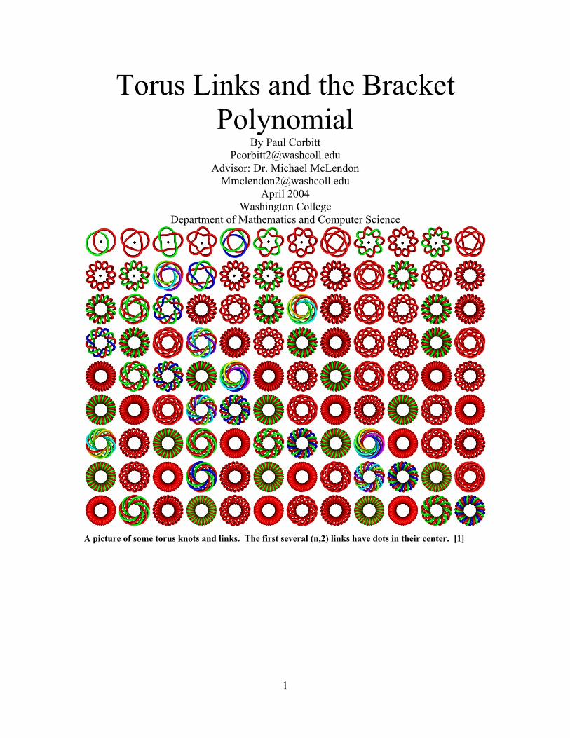
1

Torus Links and the BracketPolynomial

By Paul CorbittPcorbitt2@washcoll.edu

Advisor: Dr. Michael McLendonMmclendon2@washcoll.edu

April 2004Washington College

Department of Mathematics and Computer Science

A picture of some torus knots and links. The first several (n,2) links have dots in their center. [1]

2

Table of Contents

Abstract 3Chapter 1: Knots and Links 4

History of Knots and Links 4Applications of Knots and Links 7Classifications of Knots 8

Chapter 2: Mathematics of Knots and Links 11Knot Polynomials 11Developing the Bracket Polynomial 14

Chapter 3: Torus Knots and Links 16Properties of Torus Links 16Drawing Torus Links 18Writhe of Torus Link 19

Chapter 4: Computing the Bracket PolynomialOf (n,2) Links 21

Computation of Bracket Polynomial 21Recurrence Relation 23

Conclusion 27

Appendix A: Maple Code 28Appendix B: Bracket Polynomial to n=20 29Appendix C: Braids and (n,2) Torus Links 31Appendix D: Proof of Invariance Under R III 33

Bibliography 34Picture Credits 35

3

Abstract

In this paper torus knots and links will be investigated. Links is a more generic

term than knots, so a reference to links includes knots. First an overview of the study of

links is given. Then a method of analysis called the bracket polynomial is introduced. A

specific class called (n,2) torus links are selected for analysis. Finally, a recurrence

relation is found for the bracket polynomial of the (n,2) links. A complete list of sources

consulted is provided in the bibliography.

4

Chapter 1: Knots and Links

Knot theory belongs to a branch of mathematics called topology. Topology is a

relatively new area of mathematics; it only began to develop in the nineteenth century.

Topology is concerned with objects that can be

continuously deformed from one object to

another. The field is sometimes called rubber

sheet geometry. An illustrative example is the

fact that topologically a torus (a donut) is

equivalent to a mug (see Figure 1). A mug can

be compacted and then massaged around to

resemble a torus. The hole rather than the geometry is what relates them.

Knot theory is the subdivision of topology concerning entwined circles. A knot is

a single knotted circle, while a link is composed of two or more entangled circles. The

generic term link will refer to both knots and links; where a distinction is needed it will

be provided. The main question in knot theory is: are two knots equivalent? If we can

take one knot and deform it without any self-intersections into another knot, then the two

knots are equivalent. Failure to transform one knot into another does not mean the two

are not equivalent; perhaps a few more moves will solve the problem. Knot theory may

appear an idle academic pursuit but it has practical applications.

1.1 The History of Knots and Links

Figure 1.1 Torus and Mug.

5

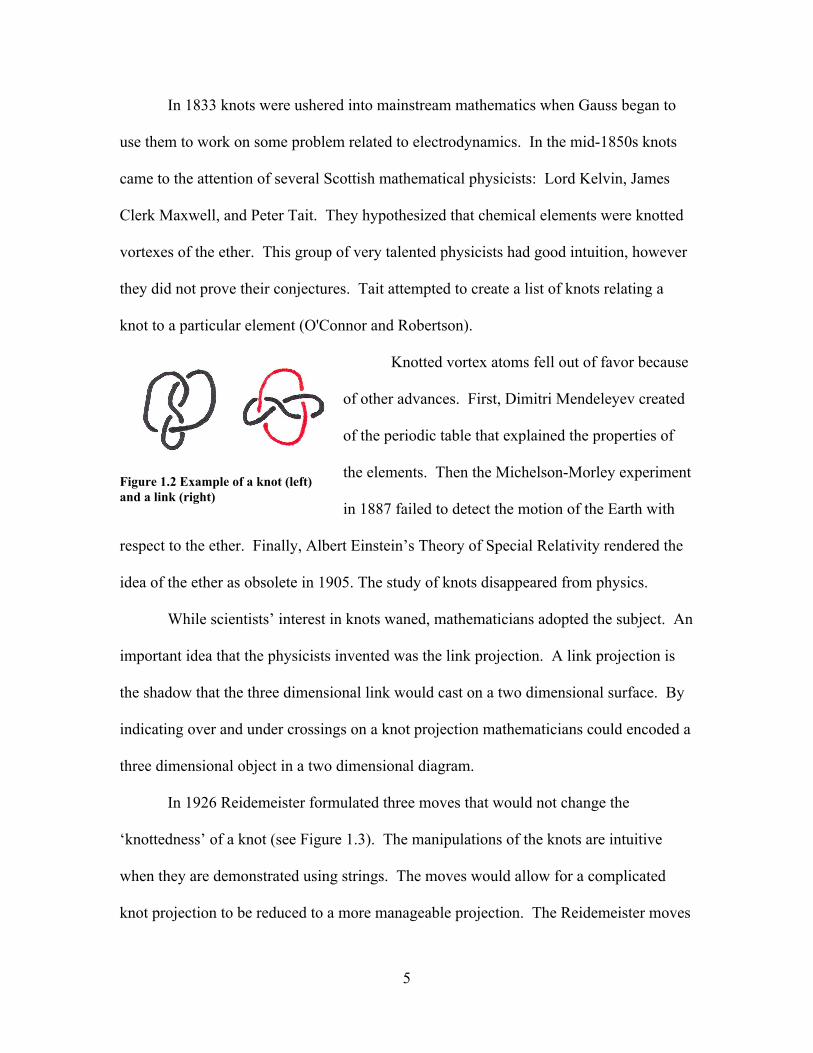
In 1833 knots were ushered into mainstream mathematics when Gauss began to

use them to work on some problem related to electrodynamics. In the mid-1850s knots

came to the attention of several Scottish mathematical physicists: Lord Kelvin, James

Clerk Maxwell, and Peter Tait. They hypothesized that chemical elements were knotted

vortexes of the ether. This group of very talented physicists had good intuition, however

they did not prove their conjectures. Tait attempted to create a list of knots relating a

knot to a particular element (O'Connor and Robertson).

Knotted vortex atoms fell out of favor because

of other advances. First, Dimitri Mendeleyev created

of the periodic table that explained the properties of

the elements. Then the Michelson-Morley experiment

in 1887 failed to detect the motion of the Earth with

respect to the ether. Finally, Albert Einstein’s Theory of Special Relativity rendered the

idea of the ether as obsolete in 1905. The study of knots disappeared from physics.

While scientists’ interest in knots waned, mathematicians adopted the subject. An

important idea that the physicists invented was the link projection. A link projection is

the shadow that the three dimensional link would cast on a two dimensional surface. By

indicating over and under crossings on a knot projection mathematicians could encoded a

three dimensional object in a two dimensional diagram.

In 1926 Reidemeister formulated three moves that would not change the

‘knottedness’ of a knot (see Figure 1.3). The manipulations of the knots are intuitive

when they are demonstrated using strings. The moves would allow for a complicated

knot projection to be reduced to a more manageable projection. The Reidemeister moves

Figure 1.2 Example of a knot (left)and a link (right)

6

will be referred to as R I, R II, and R III.

Reidemesiter recognized that a knot did not

change under planar isotopy. Planar isotopy

deforms a knot projection by altering the loops

while leaving the crossings alone.

In the late 1920s Alexander discovered

the first polynomial knot invariant. The

Alexander polynomial is a Laurent polynomial

with positive and negative powers of the variable t. The Alexander polynomial is useful

for telling knots apart. Polynomials continue to play an important role in knot theory.

The next major advance was by John Conway in the 1970s. Conway developed a

polynomial that could be used to easily obtain the Alexander polynomial. The Conway

polynomial was computed using a skein relation. Skein relation is one of the most used

tools in computing knot polynomials. A full explanation will be given when discussing

polynomials in sections 2.2 and 2.3.

In the early 1980s V.F.R. Jones made a connection between the operator algebras

that he was researching and knots. He created the Jones polynomial, a new knot

invariant. It is stronger than the Alexander polynomial in that it is able to distinguish

more knots. After Jones’ discovery, many new of polynomial invariants were

discovered. Many of these new polynomials are related or can be converted into the

Jones polynomial.

Figure 1.3 The Reidemesiter moves.

I

II

III

7

A simple polynomial is the bracket polynomial

discovered by Louis Kauffman. He saw a connection

between a physical model and knots. The bracket

polynomial is based on a skein relation, which is why it is

easy to calculate. This will be covered in greater detail in section 2.3. The Jones

polynomial is related to the bracket polynomial.

1.2 Applications of Knots

Knots find application in both pure mathematics and actual physical structures.

Often times the knots are able to offer new insight into an object that was previously not

well understood. Other times knots suggests new structures.

Once a knot is understood, it can be used to explain properties of three manifolds

encountered in topology, which would otherwise be impossible to visualize. Basing three

manifolds on knots also would allow one to know if two three manifolds are the same.

Knots are also interesting in their own right. Knot theory is also a popular branch of

modern mathematics because it is so accessible to a general audience.

In biology knots occur in the ribbon like structure DNA.

This makes it possible for a molecule of DNA to knot.

Molecules of DNA are large; this allows them to have the

necessary stretching and bending abilities to form knots. Using

knot theory biologists are able to predict what more complex

structures will look like. Researchers tested such predictions

and found that they hold true. To experimentally verify the

results they examine knotted DNA using scanning electron microscopes (see Figure 1.5).

Figure 1.4 The unknot

Figure 1.5 Knotted DNA.[2]

8

Chemists are also interested in knotted molecules. The properties of a molecule

that is unknotted and one that is knotted may be vastly different even if they are both

composed of exactly the same atoms. When creating knotted atoms it is possible to make

both a knot and its mirror image. If the knot and its mirror image are not equivalent

under Reidemeister moves and planar isotopy they are said to be chiral. The major

hurdle is that the creation of knotted molecules is difficult. The problem lies in being

able to twist the bonds between atoms to form a knot. This requires any knotted

molecule to be fairly large. The idea of knots as a model made of sticks (discussed

below) is especially appropriate for chemical applications. Chemist also have to design

the molecule and what elements go into it, as well as how to get the atoms to bond in an

appropriate way. Such challenges fuel chemists’ interest in knots.

Another major field that at first glance seem unrelated to knots is statistical

mechanics. This is a branch of physics that models the behavior of a large number of

particles. Often times a system is modeled with a lattice structure. Louis Kauffman and

other knot theorists have found connections between certain models in statistical

mechanics and knots. At this point in time statistical mechanics has provided insight into

knot theory, but knot theory has not yet contributed to statistical mechanics. It is certain

these two fields will remain closely related.

1.3 Classification of Knots

There are two major classes of knots: tame knots and wild knots. Wild knots are

knots that are not piecewise linear. So a wild knot may have smaller and smaller knotting

that shrinks down into a point. Wild knots have bizarre behaviors that make them

difficult to analyze (see Figure 1.6). The study of knots focuses on tame knots. Tame

9

knots are piecewise linear. It is easy to think of knots in terms of sticks. It is also

possible to create minimal stick models using as few sticks as possible (see Figure 1.6).

Finding the minimal stick model gives us a measure of the complexity of the knots.

Links are identified by the number of components that they have. Knots are a

special subset of links, namely links with a single component. Another characteristic

used to identify knots and links are the number of crossings of a particular projection. A

few knots have special names (see Figure 1.7). Knot theorists look for a projection of the

knot that has the minimal number of crossings. They do this because, in a sense, these

projections depict the simplest representation of that knot. Knot theorists have many

other techniques that can be deployed to understand knots.

Figure 1.6 (L to R) A wild knot [3], A minimal stick model of the trefoil [4], A stick model of thetrefoil [5]

10

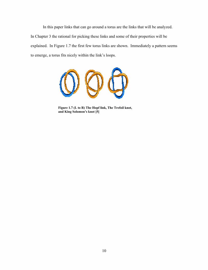
In this paper links that can go around a torus are the links that will be analyzed.

In Chapter 3 the rational for picking these links and some of their properties will be

explained. In Figure 1.7 the first few torus links are shown. Immediately a pattern seems

to emerge, a torus fits nicely within the link’s loops.

Figure 1.7 (L to R) The Hopf link, The Trefoil knot,and King Solomon’s knot [5]

11

Chapter 2: Mathematics ofKnots and Links

At first glance knots might seem to have little or no

connection to mathematics. The connections to mathematics

arise through algebraic topology along with other branches of topology. Concepts from

algebraic topology lead to major advances in knot theory. The most successful

mathematical constructs come in the form of polynomials derived from a link’s

projection.

One physical invariant that is useful is the number of components a link has. A

knot has only one component, but when looking at links the number of components is

somewhat important. A link with two components cannot become a link with three

components. This scheme is useful for initially sorting a number of knots and links.

2.1 Knot Polynomials

Knot theorists have developed several polynomials for distinguishing one knot

from another. Polynomials are much stronger than the physical features of a knot

projection, and as of yet none are foolproof. Knot theorist will continue to search for

better invariants.

Most polynomial invariants are obtained via skein relations. The skein relations

are defined in terms of the knot projection. Specific skein relations are particular to a

polynomial. Some polynomials are not

invariant under the type I Reidemeister

move, so they are referred to as framed

Figure 2.8 BorromeanRings

Figure 2.9 A type I move when viewing theknot as made of a ribbon.

12

polynomials. This means that instead of being thought of as strings they are better

thought of as ribbons though the analysis remains very much the same. These

polynomials are Laurent polynomials. They have one or more variables that can take on

both positive and negative powers. Orientation gives the link an arrow associated with

each of its components. The most discriminating polynomials often have two variables.

In recent years, many polynomials have been discovered. Some are tedious to calculate

while others are straightforward. Most of the polynomials are very similar.

The first polynomial developed was the Alexander polynomial. This polynomial

was expressed in powers of t_. This polynomial is often described in terms of the

determinant of a matrix. Being the oldest polynomial, it is well understood in terms of

algebraic topology. Work by John Conway in the late 1960s and early 1970s found an

easier way to calculate the Alexander polynomial. The problem with the Alexander

polynomial is that it is unable to distinguish between some knots.

An important part of identifying a knot was the use of skein relation in the 1960s,

again work by John Conway. These are the major tools in many of the latest

polynomials.

The next

polynomial was

discovered by V.F.R.

Jones in the early 1980s

and generalized by a number of mathematicians. Adopting Lickorish and Millets

designations for polynomials, the Jones polynomial is denoted by V(L) and the

generalized Jones polynomials P(L). The polynomial P(L) is stronger than the original

Figure 2.10 A skein relation. (L to R) The original crossing, a ‘flip’,the last two are smoothings.

13

Jones polynomial because it has two variables. The generalized polynomial can be

converted into the Jones polynomial but an appropriate change of variables. Both of

these polynomials are rather difficult to calculate.

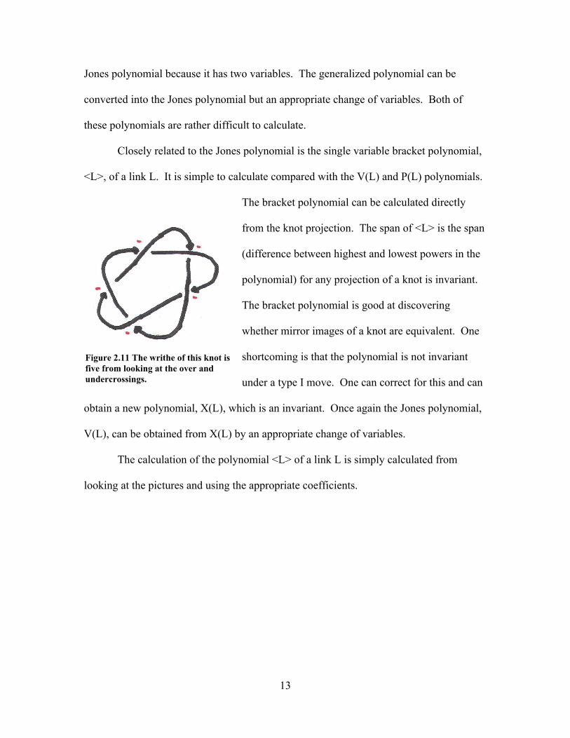
Closely related to the Jones polynomial is the single variable bracket polynomial,

<L>, of a link L. It is simple to calculate compared with the V(L) and P(L) polynomials.

The bracket polynomial can be calculated directly

from the knot projection. The span of <L> is the span

(difference between highest and lowest powers in the

polynomial) for any projection of a knot is invariant.

The bracket polynomial is good at discovering

whether mirror images of a knot are equivalent. One

shortcoming is that the polynomial is not invariant

under a type I move. One can correct for this and can

obtain a new polynomial, X(L), which is an invariant. Once again the Jones polynomial,

V(L), can be obtained from X(L) by an appropriate change of variables.

The calculation of the polynomial <L> of a link L is simply calculated from

looking at the pictures and using the appropriate coefficients.

Figure 2.11 The writhe of this knot isfive from looking at the over andundercrossings.

14

2.2 Developing the Bracket Polynomial

The bracket polynomial is chosen because it is easy to calculate. This polynomial

based on a simple skein

relation, which takes a

crossings and smoothing

them (see Figure 2.5).

There are two ways to

smooth a crossing depending

on the whether it is a positive

or negative crossing. ‘Right

handed’ knots have positive

crossings while ‘left handed’ knots have negative crossings. A smoothing removes one

crossing and creates two possible projections of the knot. This process continues until

the projection of a disjoint union of unknots. The other two rules are then applied (see

Figure 2.6).

To make the

bracket polynomial

invariant under

Reidemeister moves we

select R II and show that

the skein relation is an

invariant. Following the

proof in Figure 2.7 to be invariant AB = 1 and A2 + ABd + B2 = 0. So A = A and B = A-

Figure 2.5 Rules for smoothings to obtain the bracketpolynomial.

Figure 2.7 A pictorial proof that the bracket polynomial isinvariant under R II move.

Figure 2.6 Therules for concerning unknots.

15

1 (Kauffman p.206). Then from this relation we can conclude the d = -A4-A-4. A similar

proof can be constructed to show that these rules are invariant under the R III move (see

Appendix D). In section 4.1 the bracket polynomial of torus knots will be calculated

from these rules.

The bracket polynomial is not invariant under R I. So the bracket polynomial is a

framed invariant. The span, the lowest power subtracted from the highest power of the

polynomial, is invariant. To make it invariant it must be multiplied by the writhe of the

link, w(L), which will be discussed in Section 3.3. The bracket polynomial can also be

made invariant by multiplying <L> by A-3w(L). The X(L) polynomial is defined as X(L)

= A-3w(L)<L>.

With a wide array of invariants to chose from it is difficult to pick out which one

to use. In this case the bracket polynomial is selected. The reason is twofold; first it is

easy to calculate and second, it is good at distinguishing mirror images. The next

question is what kind of knots to study?

16

Chapter 3: Torus Knots and Links

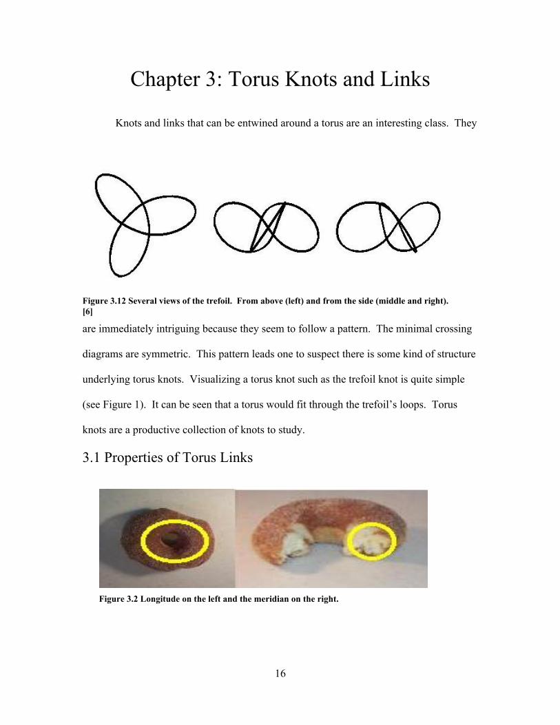
Knots and links that can be entwined around a torus are an interesting class. They

are immediately intriguing because they seem to follow a pattern. The minimal crossing

diagrams are symmetric. This pattern leads one to suspect there is some kind of structure

underlying torus knots. Visualizing a torus knot such as the trefoil knot is quite simple

(see Figure 1). It can be seen that a torus would fit through the trefoil’s loops. Torus

knots are a productive collection of knots to study.

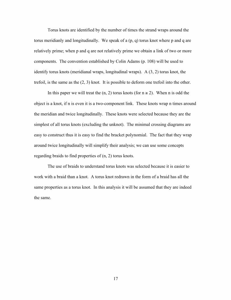
3.1 Properties of Torus Links

Figure 3.12 Several views of the trefoil. From above (left) and from the side (middle and right).[6]

Figure 3.2 Longitude on the left and the meridian on the right.

17

Torus knots are identified by the number of times the strand wraps around the

torus meridianly and longitudinally. We speak of a (p, q) torus knot where p and q are

relatively prime; when p and q are not relatively prime we obtain a link of two or more

components. The convention established by Colin Adams (p. 108) will be used to

identify torus knots (meridianal wraps, longitudinal wraps). A (3, 2) torus knot, the

trefoil, is the same as the (2, 3) knot. It is possible to deform one trefoil into the other.

In this paper we will treat the (n, 2) torus knots (for n ≥ 2). When n is odd the

object is a knot, if n is even it is a two-component link. These knots wrap n times around

the meridian and twice longitudinally. These knots were selected because they are the

simplest of all torus knots (excluding the unknot). The minimal crossing diagrams are

easy to construct thus it is easy to find the bracket polynomial. The fact that they wrap

around twice longitudinally will simplify their analysis; we can use some concepts

regarding braids to find properties of (n, 2) torus knots.

The use of braids to understand torus knots was selected because it is easier to

work with a braid than a knot. A torus knot redrawn in the form of a braid has all the

same properties as a torus knot. In this analysis it will be assumed that they are indeed

the same.

18

3.2 Drawing Torus Links

All (n, 2) torus knots are alternating knots. With a little

imagination the torus can be deformed to have two long straight

sections and U-like sections at the ends. Then all the meridian

loops are pushed to one side so that only the two longitudes are

left on the other straight section. This will be called the braid

representation of the torus knots. Then the longitudinal loops

can be cut and the torus knot becomes a braid. It is important

to bear in mind that there is a cylinder running down the center of the braid. A (n, 2)

torus knot has n crossings caused by the knot wrapping around the meridian. The two

strands of the braid have only nontrivial crossings. There is no place in the projection

where there would be a use for the second Reidemeister move. Therefore the crossings of

such a braid must alternate.

Before going any further the concept of an orientation should be established.

Putting an arrow on a strand and following it through the

entire knot will give the desired orientation. On a link

drawn as knotted around a torus putting a point in the

center of the projection and going out and putting arrows

both in the same direction will achieve the desired

orientation. This method must be used consistently. This

will be the standard orientation in this paper; other

orientations are possible. When working with the braid representation arrows pointing in

the same direction can be placed on any two parallel components to give the standard

Figure 3.13 A deformed(7,2) torus knot. The lefthand side can be thoughtof as a braid.

Figure 3.14 Orienting a link.

19

orientation. When working with just the braid it suffices to put directional arrows

pointing down from the top of the braid.

3.3 Writhe of Torus Links

Another important concept to formally define is the writhe of a link. The writhe

informally is a measure of the ‘twistedness’ of the link. In the case of a torus knot it also

tells the ‘handedness’. A positive writhe means a right-handed knot a negative writhe

mean a left-handed knot. The writhe is determined by finding whether a crossing is a

postive or negative crossing as determined by the orientation of the knot. A right hand

rule is used to establish the sign of a crossing. Point the thumb along the overcrossing

and curl the fingers. If the fingers curl in the direction of the undercrossing it is a

positive crossing. When the fingers curl against the direction of the undercrossing it is a

negative crossing. The sum of the positive and negative crossings is the writhe. The

writhe of a link is indicated by w(L).

After examining several (n, 2) knots it seems that they all have a writhe ±n. At an

intuitive level this means that all the crossings of a torus knot are the same. Combined

with the fact that torus knots are alternating, the concept of the torus knot as a braid, and

the orientation of the braid, an argument can be constructed to support this conjecture.

Figure 3.15 The writhe of the first few torus links. These are left-handed so add up the negativesigns.

20

We can consider a torus link to be made up of ‘unit

braids’ (my terminology) that are either left or right-

handed (see Firgure 6). We can then connect unit braids

together to create a torus link. The braids must be either

all left-handed (negative) or right-handed (positive). If

this was not the case the opposite braids would create a

situation where an R II move would eliminate both crossings. So all crossings are of the

same sign then the writhe is the sum of the number of crossings.

The ability to calculate the writhe allows the construction of an invariant

polynomial from the bracket polynomial. It is also interesting to note the relation that

braids have with an (n, 2) torus knot. These facts are useful for extracting information

from the projection of a torus knot.

Figure 3. 16 Left and right-handed ‘unit braids’.

21

Chapter 4: Computing the BracketPolynomial of (n,2) Links

The (n, 2) torus knots are simpler to study than most knots,since they are easy to

draw and visualize. They also exhibit some symmetry because they wrap around a torus.

Intuitively a pattern should appear when a particular invariant is calculated for various

torus knots. Once a pattern is found it can then be exploited to reach results that are

normally unobtainable.

4.1 Computation of Bracket Polynomial

Calculations can be sped up in a number of ways. First it is helpful to begin with

the simplest knots. Then as more complex knots are examined they reduce into a knot

whose bracket polynomial has already been found.

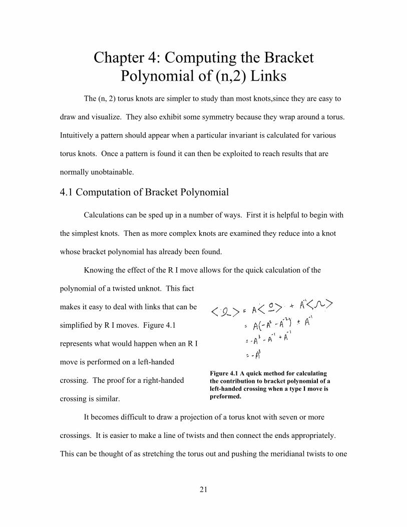
Knowing the effect of the R I move allows for the quick calculation of the

polynomial of a twisted unknot. This fact

makes it easy to deal with links that can be

simplified by R I moves. Figure 4.1

represents what would happen when an R I

move is performed on a left-handed

crossing. The proof for a right-handed

crossing is similar.

It becomes difficult to draw a projection of a torus knot with seven or more

crossings. It is easier to make a line of twists and then connect the ends appropriately.

This can be thought of as stretching the torus out and pushing the meridianal twists to one

Figure 4.1 A quick method for calculatingthe contribution to bracket polynomial of aleft-handed crossing when a type I move ispreformed.

22

side. This is the connection between knots and braids as well as how (n, 2) knots wraps

around the torus.

The bracket polynomial demonstrates that the two mirror images are distinct. In a

sense mirror images are opposites of one another. If the braid portion of a right-handed

knot is added to the left-handed knot the trivial braid is the result. If we know either the

left or right-handed bracket polynomial substituting in A-1 for A the other’s bracket

polynomial will be obtained.

Initially the rules depicted

in Figure 2.5 are applied then the

method shown in Figure 4.1 and

previous knowledge is enough to

obtain the polynomial of any

torus link. The bracket

polynomial for the Hopf link is

symmetric and requires only one

smoothing. It can then be made

into the unknot by R I (see Figure

4.1). The left-handed trefoil is

smoothed once. One smoothed

projection is the Hopf link and the

other a twisted unknot. The

twisted unknot can be calculated using the R I (see Figure 4.1) and the bracket

polynomial of the Hopf Link is complete. Combining these with the rules from section

Figure 4.2 Calculating the bracket polynomial for the lefthanded Hopf Link, Trefoil, and (4,2) link.

23

2.2, the trefoil’s polynomial is found. A left-handed (4,2) once smoothed gives a twisted

unknot and a left trefoil. Using the methods depicted in Figure 4.1 and the knowledge of

the trefoil the bracket polynomial of the (4,2) torus link is known

A few other observations are in order. In the bracket polynomial the difference

between one polynomial’s power and the next seems to be four in all cases except the

terms that come from the polynomial of the Hopf link. The difference between the

highest and lowest powers in the case of the Hopf link is eight. It stands to reason that

this is what causes mirror images of the (n, 2) torus knots not to be symmetric. If that is

the case it explains why the Hopf link is equivalent to its mirror image, but no others are.

The polynomial of (n, 2) torus knots has n terms. Also when n is even all the powers in

the polynomial are even. When n is odd the powers are all odd. The reason for this can

be understood in terms of the recurrence relation.

4.2 Recurrence Relation

Why would we want to find a formula to calculate the bracket polynomial? When

calculating the bracket polynomial for the simple knots up to about 7 crossings a pattern

emerges. Beyond that point the pictures become difficult to draw. The knot’s bracket

polynomial reduces to a twisted unknot and the previous (n-1, 2) torus knot. This pattern

seems like a ‘ladder’; once one polynomial is known we can then construct the next one.

The ‘ladder’ pattern readily suggests that a recurrence relation may be a good way to

create a formula for the (n, 2) torus knots.

24

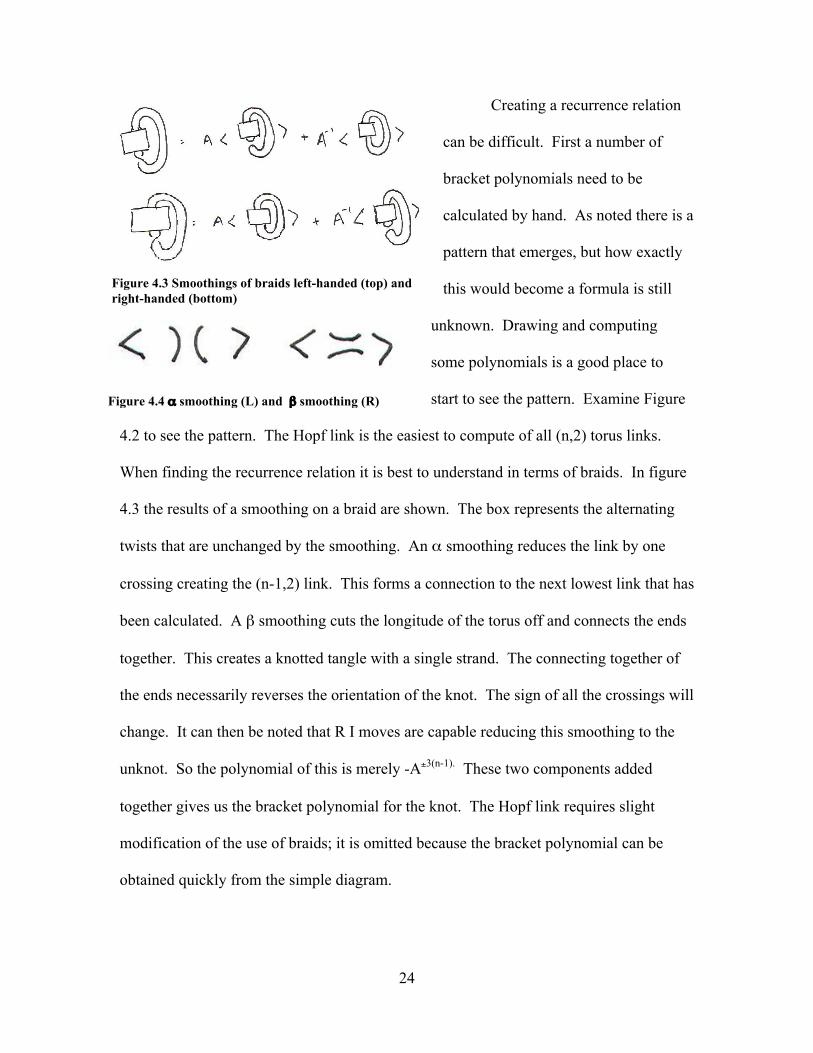
Creating a recurrence relation

can be difficult. First a number of

bracket polynomials need to be

calculated by hand. As noted there is a

pattern that emerges, but how exactly

this would become a formula is still

unknown. Drawing and computing

some polynomials is a good place to

start to see the pattern. Examine Figure

4.2 to see the pattern. The Hopf link is the easiest to compute of all (n,2) torus links.

When finding the recurrence relation it is best to understand in terms of braids. In figure

4.3 the results of a smoothing on a braid are shown. The box represents the alternating

twists that are unchanged by the smoothing. An α smoothing reduces the link by one

crossing creating the (n-1,2) link. This forms a connection to the next lowest link that has

been calculated. A β smoothing cuts the longitude of the torus off and connects the ends

together. This creates a knotted tangle with a single strand. The connecting together of

the ends necessarily reverses the orientation of the knot. The sign of all the crossings will

change. It can then be noted that R I moves are capable reducing this smoothing to the

unknot. So the polynomial of this is merely -A±3(n-1). These two components added

together gives us the bracket polynomial for the knot. The Hopf link requires slight

modification of the use of braids; it is omitted because the bracket polynomial can be

obtained quickly from the simple diagram.

Figure 4.3 Smoothings of braids left-handed (top) andright-handed (bottom)

Figure 4.4 α smoothing (L) and β smoothing (R)

25

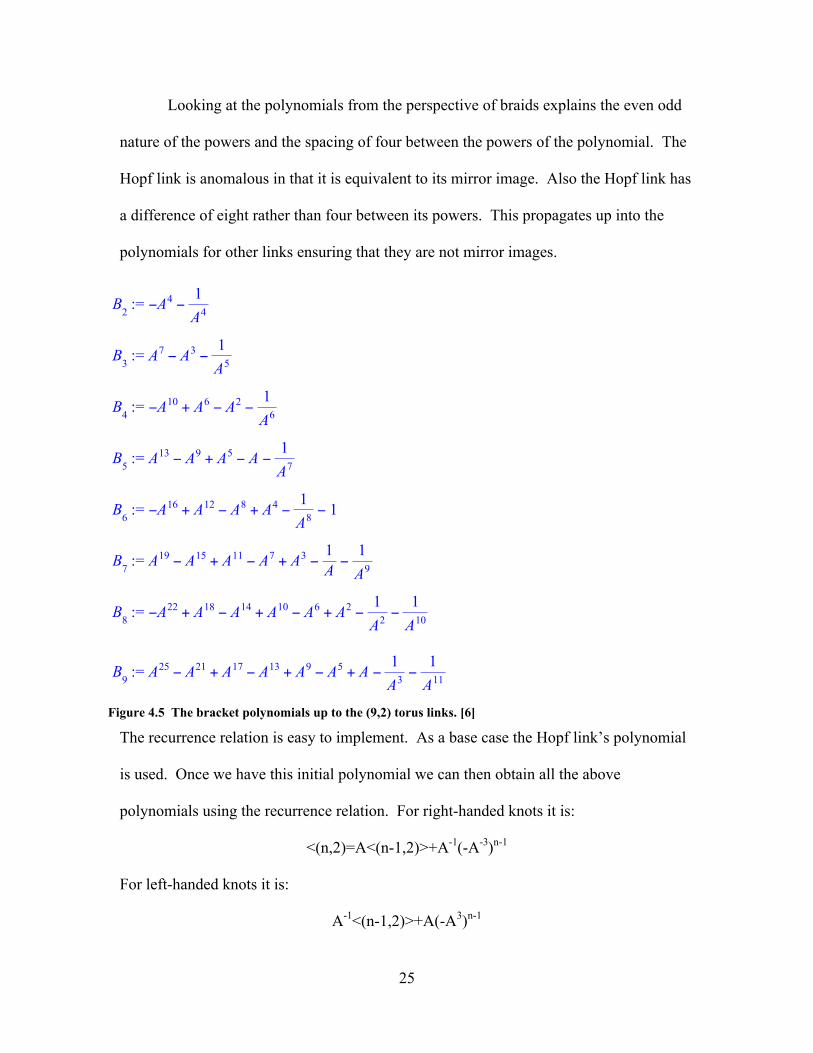
Looking at the polynomials from the perspective of braids explains the even odd

nature of the powers and the spacing of four between the powers of the polynomial. The

Hopf link is anomalous in that it is equivalent to its mirror image. Also the Hopf link has

a difference of eight rather than four between its powers. This propagates up into the

polynomials for other links ensuring that they are not mirror images.

The recurrence relation is easy to implement. As a base case the Hopf link’s polynomial

is used. Once we have this initial polynomial we can then obtain all the above

polynomials using the recurrence relation. For right-handed knots it is:

<(n,2)=A<(n-1,2)>+A-1(-A-3)n-1

For left-handed knots it is:

A-1<(n-1,2)>+A(-A3)n-1

:= B2

− − A4 1

A4

:= B3

− − A7 A3 1

A5

:= B4

− + − − A10 A6 A2 1

A6

:= B5

− + − − A13 A9 A5 A1

A7

:= B6

− + − + − − A16 A12 A8 A4 1

A81

:= B7

− + − + − − A19 A15 A11 A7 A3 1A

1

A9

:= B8

− + − + − + − − A22 A18 A14 A10 A6 A2 1

A2

1

A10

:= B9

− + − + − + − − A25 A21 A17 A13 A9 A5 A1

A3

1

A11

Figure 4.5 The bracket polynomials up to the (9,2) torus links. [6]

26

Appendix A shows the implementation of the recurrence relation. Appendix B provides

the bracket polynomial up to the (20,2) torus link.

27

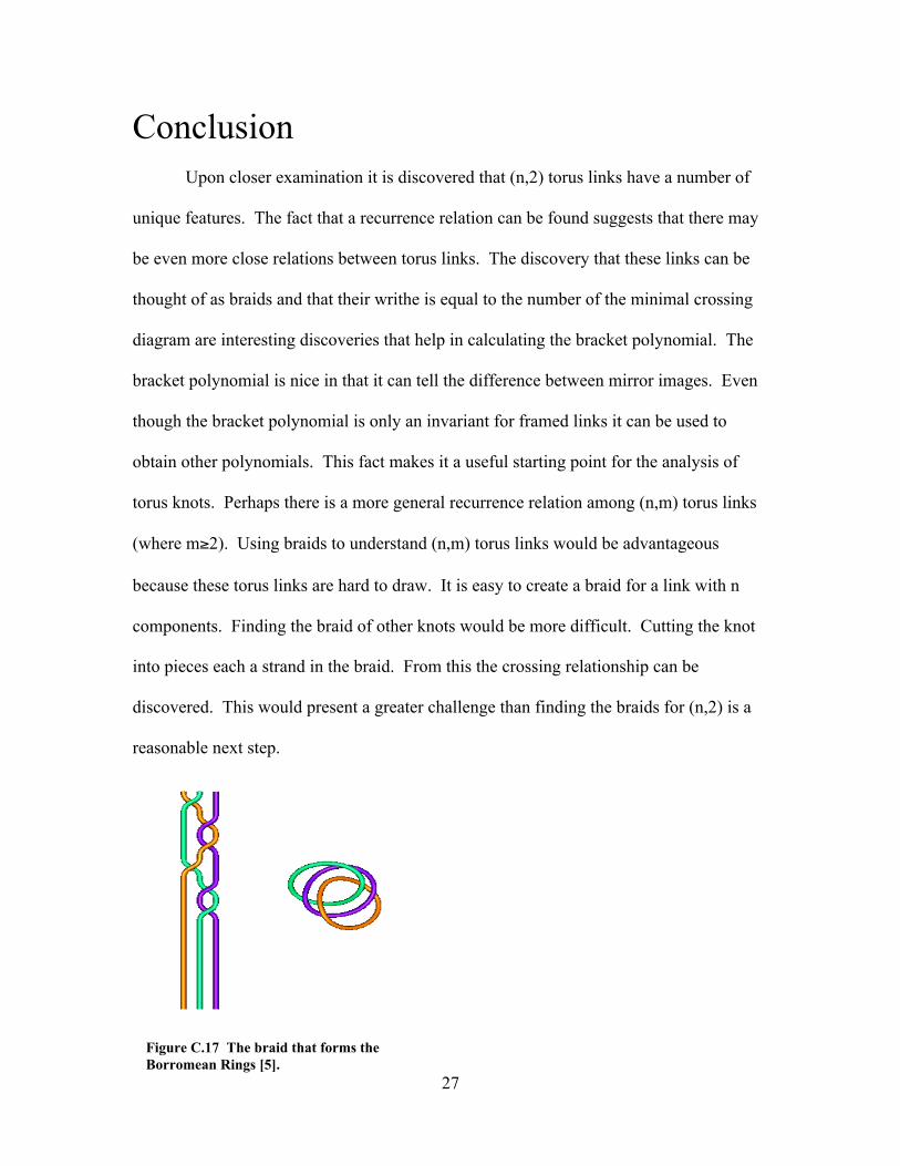
ConclusionUpon closer examination it is discovered that (n,2) torus links have a number of

unique features. The fact that a recurrence relation can be found suggests that there may

be even more close relations between torus links. The discovery that these links can be

thought of as braids and that their writhe is equal to the number of the minimal crossing

diagram are interesting discoveries that help in calculating the bracket polynomial. The

bracket polynomial is nice in that it can tell the difference between mirror images. Even

though the bracket polynomial is only an invariant for framed links it can be used to

obtain other polynomials. This fact makes it a useful starting point for the analysis of

torus knots. Perhaps there is a more general recurrence relation among (n,m) torus links

(where m≥2). Using braids to understand (n,m) torus links would be advantageous

because these torus links are hard to draw. It is easy to create a braid for a link with n

components. Finding the braid of other knots would be more difficult. Cutting the knot

into pieces each a strand in the braid. From this the crossing relationship can be

discovered. This would present a greater challenge than finding the braids for (n,2) is a

reasonable next step.

Figure C.17 The braid that forms theBorromean Rings [5].

28

Appendix A: Maple CodeThis Maple worksheet calculates the bracket polynomial for torus knots of the form (N,2)where N is a natural number greater that 3. The polynomial is found using a recurrencerelation found in the first for loop. At the bottom thier is a second loop that outputs thespan of the bracket polynomial. Note that in some places where the information thatwould be output in redundant the output is suppressed using the : symbol. Press the !!!button to execute the entire worksheet at once.This sheet was created using Maple 8 by Paul Corbitt.> restart:N controls the number of bracket polynomials to be generated from 2 up to N> N:=20;

:= N 20

Hand decribes the handedness of the knots. Hand >=0 is a right handed knot/link, hand<0 is a left handed knot/link.> Hand:=-2;

:= Hand -2

The variable k is takes the handedness of the knot for use in the calculation.> k:=-sign(Hand):<L> is the array from 2 up to N that will hold the bracket polynomial.> <L>:=array[2..N]:<L>[2] is the base step for generating all higher (i,2) knots/links.> <L>[2]:=-A^(4)-A^(-4):The for loop goes through hand calculates either right or left handed bracket polynomialsfrom 3 up to selected N.> for i from 3 to N do> <L>[i]:=sort(expand(A^(-k)*<L>[i-1]+A^(k)*(-A^(3*k))^(i-1)));> end do:Span[2..N] intializes the array holds the span of the bracket polynomial.> Span:=array[2..N]:Span[i] holds the span of the bracket polynomial B[i].> for i from 2 to N do> Span[i]:=degree(B[i])-ldegree(B[i]);> end do:

29

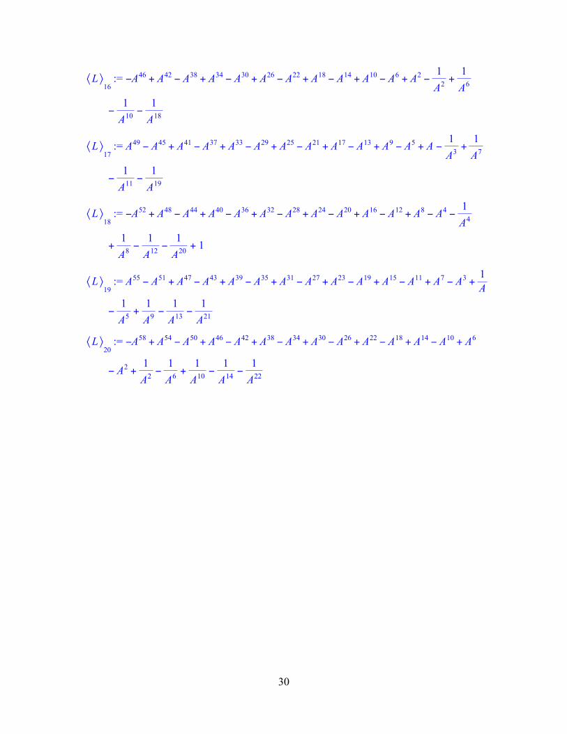
Appendix B: Bracket Polynomial to N = 20

:= 〈 〉L2

− − A4 1

A4

:= 〈 〉L3

− − A7 A3 1

A5

:= 〈 〉L4

− + − − A10 A6 A2 1

A6

:= 〈 〉L5

− + − − A13 A9 A5 A1

A7

:= 〈 〉L6

− + − + − − A16 A12 A8 A4 1

A81

:= 〈 〉L7

− + − + − − A19 A15 A11 A7 A3 1A

1

A9

:= 〈 〉L8

− + − + − + − − A22 A18 A14 A10 A6 A2 1

A2

1

A10

:= 〈 〉L9

− + − + − + − − A25 A21 A17 A13 A9 A5 A1

A3

1

A11

:= 〈 〉L10

− + − + − + − − − + A28 A24 A20 A16 A12 A8 A4 1

A4

1

A121

:= 〈 〉L11

− + − + − + − + − − A31 A27 A23 A19 A15 A11 A7 A3 1A

1

A5

1

A13

:= 〈 〉L12

− + − + − + − + − + − − A34 A30 A26 A22 A18 A14 A10 A6 A2 1

A2

1

A6

1

A14

:= 〈 〉L13

− + − + − + − + − + − − A37 A33 A29 A25 A21 A17 A13 A9 A5 A1

A3

1

A7

1

A15

:= 〈 〉L14

− + − + − + − + − + + − − − A40 A36 A32 A28 A24 A20 A16 A12 A8 A4 1

A4

1

A8

1

A161

〈 〉L15

:=

− + − + − + − + − + − + − − A43 A39 A35 A31 A27 A23 A19 A15 A11 A7 A3 1A

1

A5

1

A9

1

A17

30

〈 〉L16

A46 A42 A38 A34 A30 A26 A22 A18 A14 A10 A6 A2 1

A2

1

A6− + − + − + − + − + − + − + :=

1

A10

1

A18 − −

〈 〉L17

A49 A45 A41 A37 A33 A29 A25 A21 A17 A13 A9 A5 A1

A3

1

A7 − + − + − + − + − + − + − + :=

1

A11

1

A19 − −

〈 〉L18

A52 A48 A44 A40 A36 A32 A28 A24 A20 A16 A12 A8 A4 1

A4− + − + − + − + − + − + − − :=

1

A8

1

A12

1

A201 + − − +

〈 〉L19

A55 A51 A47 A43 A39 A35 A31 A27 A23 A19 A15 A11 A7 A3 1A

− + − + − + − + − + − + − + :=

1

A5

1

A9

1

A13

1

A21 − + − −

〈 〉L20

A58 A54 A50 A46 A42 A38 A34 A30 A26 A22 A18 A14 A10 A6− + − + − + − + − + − + − + :=

A2 1

A2

1

A6

1

A10

1

A14

1

A22 − + − + − −

31

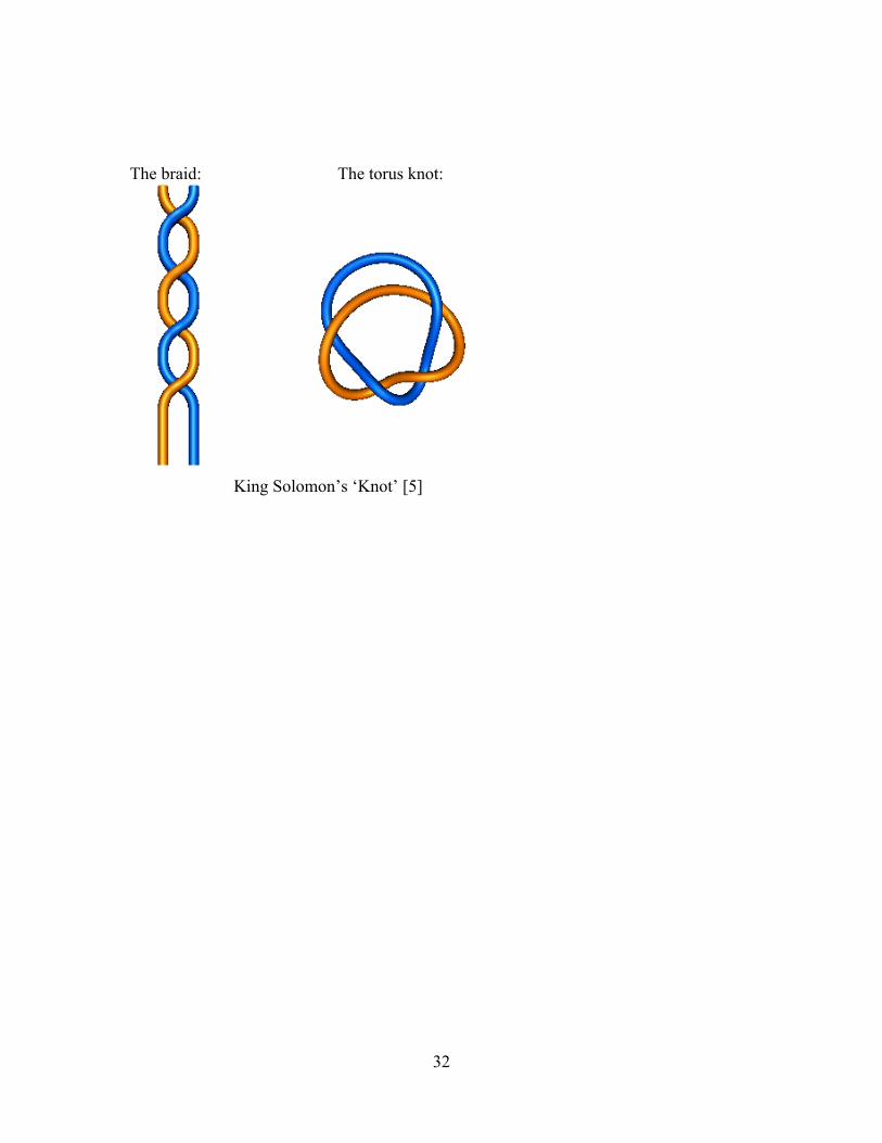
Appendix C: Braids and (n,2) Torus LinksAn easy way to imagine torus links is the idea of a braid. This discussion will

focus on (n, 2) torus knots. First create a braid with 2 strands then alternate over andunder crossings. Then connect the right top to the right bottom and the left top to the leftbottom. A (n, 2) torus knot is created. The resulting diagrams provide insight into the(n,2) torus knot. It can be noted that the n twists represent the number of times wrappedaround the meridian. The two strands that turn the braid into a knot represent the linkwrapping twice longitudinally around the torus. The following diagrams (using [5]) areexamples of the simplest (n,2) torus knots.

The braid: The torus knot:

The Hopf Link [5]

Trefoil Knot [5]

32

The braid: The torus knot:

King Solomon’s ‘Knot’ [5]

33

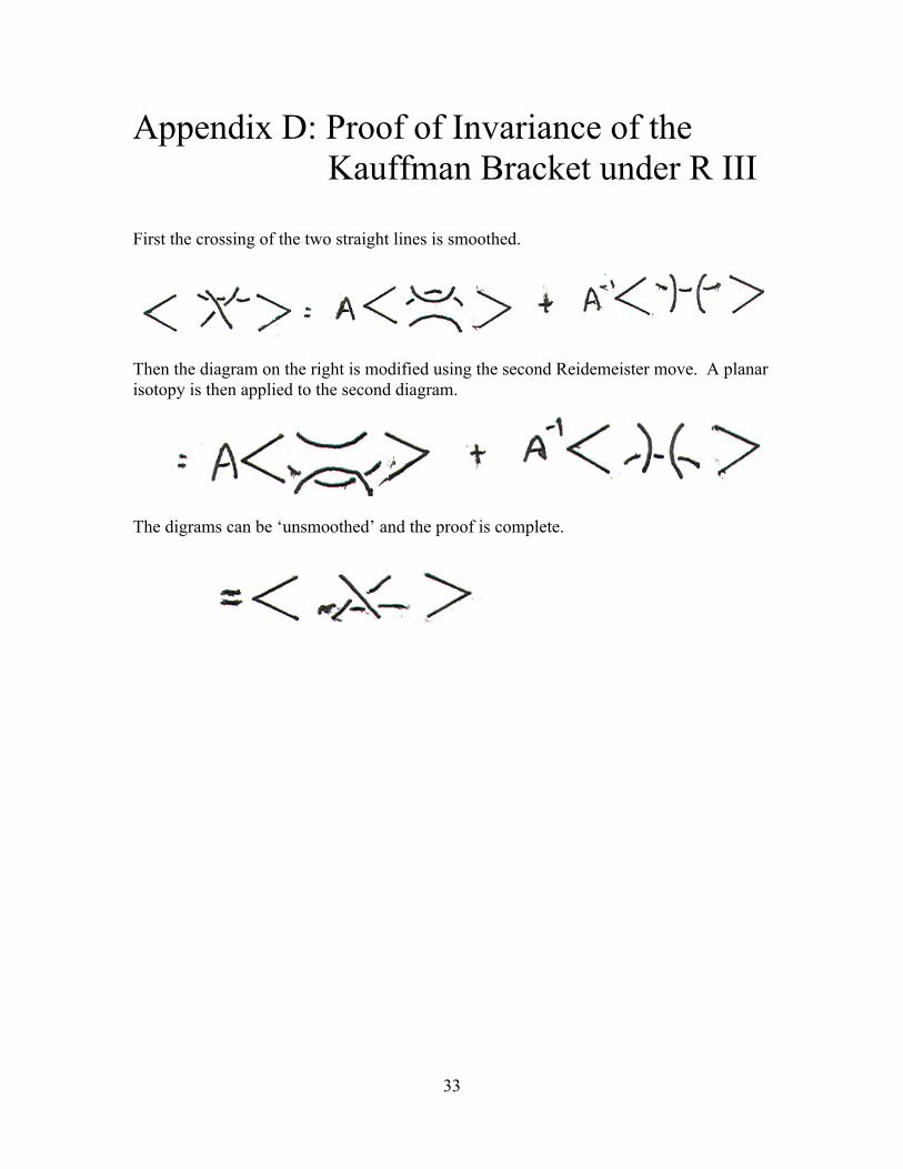
Appendix D: Proof of Invariance of the Kauffman Bracket under R III

First the crossing of the two straight lines is smoothed.

Then the diagram on the right is modified using the second Reidemeister move. A planarisotopy is then applied to the second diagram.

The digrams can be ‘unsmoothed’ and the proof is complete.

34

BibliographyAdams, Colin C. The Knot Book An Elementary Introduction to the Mathematical

Theory of Knots. 2nd ed. New York: Henry Holt, 2001.

Farmer, David W. and Theodore B. Stanford. Knots and Surfaces A Guide toDiscovering Mathematics. Providence, RI: American Mathematical Society,1996.

Kauffman, Louis H. “New Invariants in the Theory of Knots.” The AmericanMathematical Monthly Mar. 1988: 195-242.

Lickorish, W.B.R. and K.C. Millet. “The New Polynomial Invariants of Knots andLinks.” Mathematics Magazine Feb. 1988: 3-23.

O'Connor ,JJ and EF Robertson. Topology and Scottish Mathematical Physics. Jan2001 <http://www-gap.dcs.st-and.ac.uk/~history/HistTopics/Knots_and_physics.html>

Sossinsky, Alexi. Knots Mathematics With a Twist. Trans. Giselle Weiss. Cambridge:Harvard UP, 2002.

35

Picture Credits[1] ‘Torus zoo’ from:

http://www.cs.ubc.ca/nest/imager/contributions/scharein/knot-theory/torus-zoo-xing.jpg

[2] Knotted DNA from:math.rice.edu/~amheap/ interests.html

[3] A wild knot from:http://www.cs.ubc.ca/nest/imager/contributions/scharein/knot-theory/wild.pdf

[4] Picture adapted from The Knot Book on page 28.

[5] From and created using KnotPlot software and can be found at:http://www.cs.ubc.ca/nest/imager/contributions/scharein/KnotPlot.html

[6] Created using Maple 8 software.

All other figures were drawn by the author.