Torsion Points on Elliptic curves

Torsion Points on Elliptic curves

by

Darlison Nyirenda

Thesis presented in partial fulfilment of the requirements for

the degree of Master of Science in Mathematics in the

Faculty of Science at Stellenbosch University

Department of Mathematical Sciences,

University of Stellenbosch,

Private Bag X1, Matieland 7602, South Africa.

Supervisor: Dr. A. Keet

March 2013

Declaration

By submitting this thesis electronically, I declare that the entirety of the work contained

therein is my own, original work, that I am the sole author thereof (save to the extent

explicitly otherwise stated), that reproduction and publication thereof by Stellenbosch

University will not infringe any third party rights and that I have not previously in its

entirety or in part submitted it for obtaining any qualification.

2013/02/25Date: . . . . . . . . . . . . . . . . . . . . . . . . . . . . . . . . . . . .

Copyright © 2013 Stellenbosch University

All rights reserved.

i

Stellenbosch University http://scholar.sun.ac.za

Abstract

Torsion Points on Elliptic curves

D. Nyirenda

Department of Mathematical Sciences,

University of Stellenbosch,

Private Bag X1, Matieland 7602, South Africa.

Thesis: MSc

March 2013

The central objective of our study focuses on torsion points on elliptic curves. The case of

elliptic curves over finite fields is explored up to giving explicit formulae for the cardinality

of the set of points on such curves. For finitely generated fields of characteristic zero, a

presentation and discussion of some known results is made. Some applications of elliptic

curves are provided. In one particular case of applications, we implement an integer

factorization algorithm in a computer algebra system SAGE based on Lenstra’s elliptic

curve factorisation method.

ii


Opsomming

Torsiepunte op elliptiese krommes

(“Torsion Points on Elliptic Curves”)

D. Nyirenda

Departement Wiskunde,

Universiteit van Stellenbosch,

Privaatsak X1, Matieland 7602, Suid Afrika.

Tesis: MSc

Maart 2013

Die hoofdoel van ons studie is torsiepunte op elliptiese krommes. Ons ondersoek die geval

van elliptiese krommes oor ‘n eindige liggaam met die doel om eksplisiete formules vir die

aantal punte op sulke krommes te gee. Vir ‘n eindig-voortgebringde liggaam met karak-

teristiek nul bespreek ons sekere bekende resultate. Sommige toepassings van elliptiese

krommes word gegee. In een van hierdie toepassings implementeer ons ‘n heeltallige fak-

toriseringalgoritme in die rekenaar-algebrastelsel SAGE gebaseer op Lenstra se elliptiese

krommefaktoriseeringmetode.

iii


Acknowledgements

I would like to express my sincere gratitude to my surpervisor Dr. Anold Keet for his

guidance and direction. Apart from supervisory task, he introduced me to related areas

of mathematics that have been used as tools in this thesis. To that, words alone are

not enough to express my gratitude. I am grateful to Professor Florian Breuer and

Professor Stephan Wagner for introducing me to Number Theory and thus my interest

to pursue studies on the subject. I want to thank the African Institute for Mathematical

Sciences and Stellenbosch University for the scholarship that has seen me complete a

masters’ degree in Mathematics. To Professor Edward Schaefer (Santa Clara University,

USA), Professor John Ryan and Dr. Khumbo Kumwenda (Mzuzu University, Malawi),

I want to say a big thank you for realising potential in me and fighting tirelessly to let

me pursue further studies at postgraduate level. To my classmates Tovohery Hajatiana

Randrianarisoa, Evans Doe Ocansey and Frances Odumodu, thank you for social and

spiritual support not forgetting the comfortable environment you set for me. You were

true brothers and sister in a family. To the rest of friends, I say be blessed.

iv


Dedications

To my brothers Roosevelt and Vitumbiko, my sisters Tiwonge and Vynida

To my dad Joel and mum Magret

v


Contents

Declaration i

Abstract ii

Opsomming iii

Acknowledgements iv

Dedications v

Contents vi

Nomeclature viii

1 Introduction 1

2 Preliminaries 3

2.1 Affine and projective varieties . . . . . . . . . . . . . . . . . . . . . . . . 3

2.2 Maps between projective curves . . . . . . . . . . . . . . . . . . . . . . . 7

2.3 Riemann-Roch Theorem and curve genus . . . . . . . . . . . . . . . . . . 9

3 Basics of Elliptic Curves 15

3.1 The Group Law . . . . . . . . . . . . . . . . . . . . . . . . . . . . . . . . 19

3.2 Isogenies and the torsion structure . . . . . . . . . . . . . . . . . . . . . 25

3.3 Weil pairing and elliptic curves over finite fields . . . . . . . . . . . . . . 34

3.4 Characterisation of the endomorphism ring . . . . . . . . . . . . . . . . . 43

4 Elliptic curves over complex numbers 47

vi


4.1 Complex tori as elliptic curves . . . . . . . . . . . . . . . . . . . . . . . . 52

4.2 Uniformization theorem . . . . . . . . . . . . . . . . . . . . . . . . . . . 56

5 Elliptic curves over local fields 62

5.1 Formal Groups . . . . . . . . . . . . . . . . . . . . . . . . . . . . . . . . 62

5.2 Reduction . . . . . . . . . . . . . . . . . . . . . . . . . . . . . . . . . . . 72

6 Bounds on torsion points 81

6.1 The case of Fq and Q . . . . . . . . . . . . . . . . . . . . . . . . . . . . . 81

6.2 Finitely generated characteristic zero fields . . . . . . . . . . . . . . . . . 83

7 Applications of elliptic curves 93

7.1 Diffie-Hellman Key Exchange . . . . . . . . . . . . . . . . . . . . . . . . 93

7.2 Integer factorisation . . . . . . . . . . . . . . . . . . . . . . . . . . . . . . 94

8 Conclusion 97

A Computer Algebra System 99

List of References 103

vii


Nomeclature

Symbols Definitions

Z the set of integers

R the set of real numbers

Q the set of rational numbers

C the set of complex numbers

#G or |G| the cardinality of G

(xij) a matrix with the entry xij in ith row and jth column

det (xij) the determinant of a matrix (xij)

K the algebraic closure of K

Gal(L/K) the Galois group of the field L over the field K

GLn(R) the set of n× n invertible matrices whose entries belong to the ring R

bxc the greatest integer less than or equal to x

(G : H) the index of a subgroup H in a group G

charK the characteristic of a field K

R× the set of units in R

QuotR the fraction field of an integral domain R

viii


Chapter 1

Introduction

The study of polynomial systems of equations has had remarkable advancement. Of

particular class is that of Diophantine equations which are equations of the form

f(x1, x2, . . . , xn) = 0 where f ∈ Q[x1, x2, . . . , xn].

Some of the questions that may be asked include, but are not limited to, does f = 0 have

solutions in Q? If it has solutions, are they finitely many? Instead of seeking solutions

in rational numbers, we may go further by looking at solutions in the algebraic closure

Q. There is so much theory in this area and of special attention are cubic curves. A

certain class of cubic curves called elliptic curves is the focal point of our study. As

it will be shown, there is a natural group law on the curves which can be described

geometrically. The method, called chord-tangent method is used to add points on the

curves, thus giving rise to new points. So we can enumerate as many points as possible.

Since elliptic curves are algebraic, there is an extensive use of algebraic geometry tools to

arrive at certain results. The second and third chapters are devoted to some fundamental

theory of elliptic curves. We review some relevant algebraic geometry on affine and

projective varieties without going too far afield. Our focus is on the useful results that

apply to algebraic curves, especially on divisors of curves. In chapter two, the group law

is discussed. Unlike proving the associativity property of the addition law using explicit

equations, we use the theory of divisors and isogenies for the proof. The Weil pairing

is introduced and discussed since it is an important tool that is used in deducing some

results concerning elliptic curves defined over finite fields. It is also applicable in some

1


cases for elliptic curves over Q. Its properties are proved. The ring of isogenies called the

endomorphism ring of an elliptic curve is characterized in the same chapter. We present

by proof all possibilities the endomorphism ring can occur. In such a situation, we notice

that the characteristic of a field imposes a further restriction on the nature of the ring.

The endomorphism ring plays a role in determination of some known torsion bounds for

elliptic curves. Chapter four is entirely devoted to elliptic curves defined over C. The goal

of this chapter is to show that a torus is the same as an elliptic curve. More precisely, if

we start with a torus, we can construct an elliptic curve which is the ‘same’ as the torus.

Conversely, if we start with an elliptic curve, we can construct a torus which is the ‘same’

as the elliptic curve we started with. This result allows us to infer the torsion structure

of points on any given elliptic curve over C whose order divide some fixed integer. In

chapter five, we present a proof of Nagell-Lutz theorem using formal groups, an approach

that avoids complicated heavy calculations that involve moving the infinite point to a

finite point and examining the new curve. Reduction of elliptic curves is discussed in

line with formal groups and local fields. In particular, we obtain a lot of information

about the torsion subgroup of an elliptic curve over Q using reduction modulo different

primes. This information tells us about the possible size of the torsion subgroup and

together with Nagell-Lutz theorem, the group becomes manageable to determine. This

is backed by several examples that we provide. Chapter six looks at bounds on torsion

points. We give several examples verifying the theoretical results and discuss a torsion

bound due to Breuer [1]. In chapter seven, we give two applications of elliptic curves;

integer factorization and cryptographic key exchange. The subject of elliptic curves is

very broad. Some theorems are stated without proof and their results used.

2


Chapter 2

Preliminaries

The references used in this chapter are [8] and [2].

2.1 Affine and projective varieties

We look at algebraic sets in affine and projective spaces and then narrow down to algebraic

curves over an arbitrary field. Unless otherwise stated, a field is assumed to be perfect

and shall be denoted by K.

Definition 2.1.1. Affine n-space over K, denoted An is the set of n-tuples in which

components are elements of K, i.e, (x1, x2, . . . , xn) : xi ∈ K. The notation An(K) is

used for the set of all points in An with components in K.

Definition 2.1.2. The set V is said to be an affine algebraic set if there exist polynomials

f1, f2, . . . fm such that V = P ∈ An : f(P ) = 0 for 1 ≤ i ≤ m. The polynomials fi for

i ∈ 1, 2, . . . ,m are called defining polynomials of V . The vanishing ideal of V is the set

I(V ) = f ∈ K[X] : f(P ) = 0 ∀ P ∈ V

We place a topology on An in which closed sets are precisely the algebraic sets. This

topology is known as Zariski topology. We write V/K if I(V ) can be generated by

elements of K[X] and say that V is defined over K. Clearly, if defining polynomials of V

have coefficients in K, then V is defined over K. Note that for any ideal I ⊂ K[X], we

always have a finite number of generators since K[X] is Noetherian. An affine algebraic

3


set V is said to be an affine variety if I(V ) is a prime ideal of K[X], i.e K[X]/I(V ) is an

integral domain.

Given an affine variety V defined over K, we define its coordinate ring to be the set

K[V ] := K[X]/I(V ). In this case, for f, g ∈ K[X], it follows that f = g ∈ K[V ] if and

only if f − g ∈ I(V ). The function field of V , denoted by K(V ) is quotient field of K[V ].

Definition 2.1.3. Let V be an affine variety. The dimension of V , denoted by dim(V )

is the transcendence degree of K(V ) over K.

Example 2.1.4. Consider the set V = (a, b). Clearly I(V ) = 〈x − a, y − b〉. So

K[V ] = K[x,y]〈x−a,y−b〉 = K ⇒ K(V ) = K. Hence dim(V ) = 0.

Let V/K be an affine variety and consider M = g ∈ K[V ] : g(P ) = 0. Then M is

a maximal ideal of K[V ] since the map ψ : K[V ] → K defined as g 7→ g(P ) is a ring

epimorphism. We can thus localize K[V ] at its maximal ideal. Denote this localization

by OP (V ). Then, we have that

OP (V ) =

f

g: f, g ∈ K[V ], g(P ) 6= 0

.

We call OP (V ) the local ring of K[V ] at P . A function ψ ∈ K(V ) is regular or de-

fined at P ∈ V if ψ = fgfor some f, g ∈ K[V ] and g(P ) 6= 0. A point at which ψ is not

defined is a pole of ψ. For a point P , observe thatOP (V ) = ψ ∈ K(V ) : ψ regular at P.

Those functions that are regular everywhere on V are precisely K[V ]. Elements of K[V ]

can be viewed as regular (polynomial) maps from V to K ∼= A1. The definition of a

regular map can be extended to affine varieties in An for arbitrary n. Similarly, we can

define a rational map between affine varieties. We will not discuss this here, so for more

information, refer to [8].

Define a relation ∼ on An+1 \ (0, 0, . . . , 0) by (x0, x1, . . . , xn) ∼ (y0, y1, . . . , yn) if and

only if there exists λ ∈ K× such that yi = λxi for all 1 ≤ i ≤ n. Then ∼ is an equivalence

relation. We call the set

Pn := (An \ (0, 0, . . . , 0))/ ∼

4


the projective n-space, and denote its elements by [x0 : x1 : . . . : xn]. Consider

Ui = (x0 : x1 : . . . : xi−1 : xi : xi+1 : . . . : xn) ∈ Pn : xi 6= 0.

We can scale down the coordinates by dividing each component by xi so that elements of

Ui are of the form(x0xi

: x1xi

: . . . : xi−1

xi: 1 : xi+1

xi: . . . : xn

xi

). It is easy to see that An ∼= Ui

up to regular isomorphism. Consider the map ζi : An → Pn defined by

(x1, x1, . . . , xn) 7→ (x1 : x2 : . . . : xi−1 : 1 : xi+1 : . . . : xn).

We have ζi(An) = Ui. On the other hand, the inverse ζ−1i : Ui → An

i is realized as

(x0 : x1 : . . . : xi−1 : xi : xi+1 : . . . : xn) 7→(x0

xi,x1

xi, . . . ,

xi−1

xi,xi+1

xi, . . . ,

xnxi

).

Thus, we can embed An in Pn. So An ⊂ Pn means that the identification of An via some

ζi is assumed. Similarly, any affine variety V ⊂ An can be embedded in Pn via the above

map. The smallest closed set containing the image of V is called the projective closure of

V and is denoted by V . Given defining polynomials of V , we can find defining polynomials

of V by homogenizing and the reverse process by dehomogenizing the polynomials.

For instance, let f ∈ K[x, y, z] be the defining polynomial of V . Choose the embedding

x = XZ. Then f ? = Zdeg ff(X

Z, YZ

) is the defining polynomial for V .

We can define a projective variety and its coordinate ring of a projective variety in

the same way as done for affine varieties. However, a distinction should be noted that

vanishing ideals of projective varieties are homogeneous.

Definition 2.1.5. Let V be a projective variety. Choose An ⊂ Pn with V ∩ An 6= ∅ .

Then the function field of V is defined as

K(V ) := K(V ∩ An).

Thus K(V ) consists of functions of the form fgwhere f and g are homogeneous of the

same degree and g /∈ I(V ). Furthermore, fg

= stin K(V ) if ft−gs ∈ I(V ). If V is defined

over K, then K(V ) is defined in a similar manner. We call V a curve if it has dimension

1.

5


Definition 2.1.6. Let V be a variety with I(V ) = 〈f1, f2, . . . , fm〉. A point P ∈ V is

non-singular (smooth) if the m× n matrix(∂fi∂xj

(P )

)1≤i≤m1≤j≤n

has rank n - dim(V ). If all P ∈ V are smooth, V is said to be smooth. Otherwise, V is

singular.

If V is a curve and P ∈ V smooth, then OP (V ) is a discrete valuation ring [8]. Recall

that its unique maximal ideal is M = f ∈ K[V ] : f(P ) = 0. We define a map

ordP : OP (V )→ Z ∪ ∞ by ordP (f) = maxr : f ∈ Mr which canonically extends to

K(V ) via ordP (f−1) = −ordP (f). By convention, ordP (0) =∞. A uniformizer for V at

P is a function t ∈ K(V ) such that ordP (f) = 1. Note that any f ∈ K(V ) is such that

f = utordP (f) where u ∈ OP (V )×, and t a uniformizer at P . Thus the order of f at P is

ordP (f). If ordP (f) ≥ 0, f is regular at P . Otherwise it has a pole.

Proposition 2.1.7. Let C be a curve defined over K and t a uniformizer at a smooth

point P ∈ C. Then K(C)/K(t) is a finite separable extension.

Proof. Since t is transcendental over K, the transcendence degree of K(t) over K is 1. We

also know that K(C) has transcendence degree 1. Hence K(C)/K(t) is a finite extension.

We need to show that every y ∈ K(C) is separable over K(t). Clearly, y is algebraic

over K(t) so that y is a root of some polynomial∑

ij gi(t)Yj where gi(t) ∈ K(t). We can

multiply every gi(t) by some suitable polynomial in K[t] to clear out the denominators

and get a relation ∑ij

aijtiyj = 0.

Let f(t, Y ) =∑

i,j aijtiY j be the minimal polynomial of y overK(t). Let p = char K > 0.

If f has a non-zero term aijtiY j such that j 6= pk for some integer k ∈ Z, then ∂f

∂Y6= 0

so that y is separable over K(t). Otherwise, f(t, Y ) = g(t, Y p). Since K is perfect, every

polynomial h(t, Y ) is such that h(tp, Y p) = h(t, Y )p for some h(t, Y ) ∈ K[t, Y ]. We can

rearrange powers of t in g(t, Y p) so that

g(t, Y p) =

p−1∑l=0

(∑ij

cijltpiY pj

)tl =

p−1∑l=0

gl(t, Y )ptl.

6


Now ordP (gl(t, y)ptl) = pordP (gl(t, y)) + l ≡ l (mod p). This shows that gl(t, y)ptl’s have

distinct orders at P . Recall that f(t, y) = 0 which yields

p−1∑l=0

gl(t, y)ptl = 0. (2.1.1)

Assume that for some 0 ≤ k ≤ p− 1, gk(t, y)ptk 6= 0. Then from Equation 2.1.1, we have

gk(t, y)ptk = −p−1∑l=0l 6=k

gl(t, y)ptl

which implies that ordP (gk(t, y)ptk) = minordP (gl(t, y)ptl : l = 0, 1, . . . , p − 1 \ k.

But this contradicts the fact that orders are distinct. So we must have gl(t, y)ptl =

0 ⇒ gl(t, y) = 0 for all l = 0, 1, . . . , p − 1. At least one of the gl(t, Y )p’s, say gc(t, Y )

must involve Y . So y is a root of gc(t, Y ). However, deg gc(t, Y ) < deg f(t, Y ), gives a

contradiction to the minimality of f(t, Y ).

2.2 Maps between projective curves

From now onwards, all varieties under discussion are assumed projective.

Definition 2.2.1. Let V ⊂ Pn and W ⊂ Pm. A rational map from V to W is a map

ψ = [ψ1, ψ2, . . . , ψm] with ψi ∈ K(V ) for all 1 ≤ i ≤ m, and at all points P ∈ V where

ψi’s are regular, ψ(P ) ∈ W .

The set V (K) is clearly Gal(K/K)-invariant. We say that ψ is defined over K if ψσ = ψ,

∀σ ∈ Gal(K/K), with the usual formula ψ(P )σ = ψσ(P σ).

Definition 2.2.2. A rational map in Definition 2.2.1 is regular at P if there exists

f ∈ K(V ) such that fψi is regular at P for all i, and fψj(P ) 6= 0 for some j. If that

happens, we set ψ(P ) = [fψ1(P ), fψ2(P ), . . . , fψm(P )]. An everywhere regular rational

map is called a morphism.

Two varieties V and W are said to be isomorphic if there exist morphisms f : V → W

and g : W → V such that f g and g f are identity maps on W and V , respectively. In

this case, we write V ∼= W .

7


Proposition 2.2.3. Let V ⊂ Pn be a variety and C be a curve with a smooth point P .

Let ψ : C → V be a rational map. Then ψ is regular at P .

Proof. We can write ψ = [ψ1, ψ2, . . . , ψn] with ψi ∈ K(C). Let t be a uniformizer at

P . Set m = minr : r = ordP (ψi), 1 ≤ i ≤ n. So m = ordP (ψj) for some j. Then

ordP (t−mψi) ≥ 0 ⇒ t−mψi is regular at P for all i. Also note that ordP (t−mψj) = 0 ⇒

(t−mψj)(P ) 6= 0. This shows that ψ is regular at P.

Proposition 2.2.4. Let ψ : C1 → C2 be a morphism between curves. Then ψ is either

constant or surjective.

Proof. See [8].

For a surjective rational map ψ : C1/K → C2/K which is defined over K, the map

ψ∗ : K(C2) → K(C1) given by ψ∗(f) = f ψ is injective. We have a tower of fields

K ⊂ ψ∗K(C2) ⊂ K(C1). Since K(C1) and K(C2) are finitely generated over K with

transcendence degree 1 and using the fact that transcendence degree is additive across a

tower, it follows that [K(C1) : ψ∗K(C2)] <∞. We call ψ a finite map.

Definition 2.2.5. A non-constant morphism ψ : C1 → C2 between curves is called

separable, inseparable or purely inseparable if the extension K(C1)/ψ∗K(C2) has the

property in concern. We use degsψ to denote the separable degree and degiψ for the

inseparable degree. In all cases, we have degψ = degsψ · degiψ. We also have that ψ is

separable if and only if degiψ = 1.

Definition 2.2.6. Let ψ : C1 → C2 be a non-constant morphism of smooth curves. For

a point P ∈ C1, let t be a uniformizer of C2 at ψ(P ). We call the number

eψ(P ) := ordP (t ψ)

the ramification index of ψ at P . If eψ(P ) > 1, ψ is said to be ramified at P , otherwise

it is unramified at P . We say that ψ is unramified if it is unramified at all points.

We remark that the ramification index is independent of the choice of the uniformizer.

Say, if t′ is another uniformizer at ψ(P ), then t′

tis regular and not zero at ψ(P ). We

deduce that ordP (t′ ψ) = ordP(t t′

t ψ)

= ordP (t ψ) + ordP(t′

t ψ)

= ordP (t ψ).

8


Proposition 2.2.7. Let ψ : C1 → C2 be a non-constant morphism of smooth curves

defined over K. Then for any φ ∈ K(C2) and P ∈ C1, we have ordP (φ ψ) =

eψ(P )ordψ(P )(φ). Furthermore, if β : C2 → C3 is another non-constant morphism be-

tween curves, then eβψ(P ) = eψ(P )eβ(ψ(P )).

Proof. For the first part, let t be a uniformizer at ψ(P ). Then φ = tru where u is regular

and not zero at ψ(P ). Since ψ is regular at P , we must have u ψ regular and not zero

at P ⇒ ordP (u ψ) = 0. Clearly, ordP (φ ψ) = ordP (tr ψ) + ordP (u ψ) = reψ(P ).

For the second part, let t′ be a uniformizer at (β ψ)(P ). Then eβψ(P ) = ordP ((t′ β)

ψ) = eψ(P )ordψ(P )(t′ β) = eψ(P )eβ(ψ(P ))ord(βψ)(P )(t

′) = eψ(P )eβ(ψ(P )).

Proposition 2.2.8. Let ψ : C1 → C2 be a non-constant rational map between two

smooth curves. Then for almost all Q ∈ C2, |ψ−1(Q)| = degs(ψ) and for any Q ∈ C2, we

have ∑P∈ψ−1(Q)

eψ(P ) = deg(ψ).

Proof. Refer to [8].

By Proposition 2.2.8, it is easy to show that ψ is unramified if and only if |ψ−1(Q)| =

deg(ψ) for all Q ∈ C2.

2.3 Riemann-Roch Theorem and curve genus

Let C be a curve. A divisor on C is a formal finite sum D given by

D =∑P∈C

nP (P ) where nP = 0 for almost all P ∈ C.

We denote by Div(C) the free abelian group of divisors on C. The degree of D is the

sum∑

P∈C nP , which we denote by deg D. The divisors of degree zero form a subgroup.

We use the notation Div0(C) for the degree zero divisor group. We say that D is defined

over K if Dσ = D for all σ ∈ Gal(K/K). We define the divisor of f ∈ K(C) as

div(f) :=∑

P∈C ordP (f)(P ). D is said to be principal if there exists f ∈ K(C)× such

that D = div(f). Since∑

P ordP (f) = 0, the divisors of functions form a subgroup of

Div0(C), and the group shall be denoted by Prin(C). The divisors D1 and D2 are said

9


to be linearly equivalent, written D1 ∼ D2, if and only if D1−D2 is principal. Clearly ∼

is an equivalence relation and we set Cl(C) := Div(C)/Prin(C) and call the quotient the

divisor class group.

Definition 2.3.1. The degree-0 part of the divisor class group of C is defined to be

the quotient Cl0(C) := Div0(C)/Prin(C). The notation DivK(C) is used to emphasize

elements of Div(C) that are invariant under the action of Gal(K/K). The groups Div0K(C)

and Cl0K(C) are defined in a similar way.

Proposition 2.3.2. Let f ∈ K(C)×. Then div(f) = 0 if and only if f ∈ K×. Further-

more, deg(div(f)) = 0.

Proof. Suppose f ∈ K. Then f has no poles (or zeros) on C so that ordP (f) = 0 for all

P ∈ C. Thus div(f) = 0. Conversely, if div(f) = 0, then f has no poles (or zeros) on C.

But such a function must be constant, i.e f ∈ K×. The second part easily follows from

the fact that f is a quotient of homogeneous polynomials of the same degree, and thus

the number of poles is the same as the number of zeros (counted with multiplicity).

Definition 2.3.3. Let φ be a non-constant rational map between two smooth curves C1

and C2. Then φ induces a homomorphism φ∗ : Cl(C1)→ Cl(C2) which we defined as[∑ni(Pi)

]7→[∑

ni(φ(Pi))].

The map in Definition 2.3.3 will be useful when we consider isogenies of elliptic curves.

Definition 2.3.4. A divisor D =∑

P∈C nP (P ) is called effective (or positive) if nP ≥ 0

for all P ∈ C. In such case we write D ≥ 0. On the same note, D1 ≥ D2 indicates that

D1 −D2 is effective.

For a divisor D, define

L(D) = f ∈ K(C)× : div(f) ≥ −D ∪ 0.

Note that L(D) is a tool for describing zeros or poles of functions. For instance, if

D = 3(P )− (Q), then f ∈ L(D) means that f can only have a pole of order at most 3 at

P and has a zero at P of order at least 1. Note that f has no pole at all points not equal

to P .

10


Proposition 2.3.5. Let D ∈ Div(C). Then L(D) is a vector space over K.

Proof. Let f1, f2 ∈ L(D). Then for c1, c2 6= 0, we have

div(c1f1 + c2f2) =∑P∈C

ordP (c1f1 + c2f2)(P )

≥∑P∈C

minordP (c1f1), ordP (c2f2)(P )

≥ −D.

The case cf with c ∈ K, f ∈ K(C)× is not difficult. All the vector space axioms easily

follow.

We denote the dimension of L(D) by l(D). If C is defined over K and D ∈ DivK(C),

then L(D) has a generating set with functions in K(C), see [8].

Definition 2.3.6. For a curve C, the collection of differential forms ΩC is the vector

space over K whose generating set consists of symbols of the form df where f ∈ K(C).

The space has the following properties:

a. d(f + g) = df + dg for all f, g ∈ K(C).

b. d(fg) = fdg + gdf for all f, g ∈ K(C).

c. da = 0 for all a ∈ K.

Let φ : C1 → C2 be a non-constant morphism between curves. The corresponding map

on function fields φ∗ : K(C2)→ K(C1) induces the following map on differential forms:

φ∗ : ΩC2 → ΩC1 defined by(∑

fidyi

)7→∑

φ∗(f)d(φ∗yi).

Proposition 2.3.7. Let C be a curve.

a. dimK(C)ΩC = 1.

b. Let y ∈ K(C). Then dy is a basis if and only if K(C)/K(y) is separable.

c. Suppose φ : C1 → C2 is a non-constant morphism. Then φ∗ : ΩC2 → ΩC1 is

one-to-one if and only if φ is separable.

11


Proof. For (a) and (b), see [8].

(c). Choose y ∈ K(C2) such that dy is a basis for ΩC2 . We know that φ∗ : K(C2)→ K(C1)

is injective since φ is surjective. By (b), K(C2)/K(y) is separable. Now by the identi-

fications K(C2) ∼= φ∗K(C2) and K(y) ∼= φ∗K(y), it follows that φ∗K(C2)/φ∗K(y) =

φ∗K(C2)/K(φ∗y) is separable.

Suppose φ∗ is injective. Then φ∗(dy) = d(φ∗y) 6= 0 ⇒ d(φ∗y) is a basis for ΩC1 ⇒

K(C1)/K(φ∗y) = K(C1)/φ∗K(y) is separable ⇒ K(C1)/φ∗K(C2) is separable since

φ∗K(C2)/φ∗K(y) is separable as shown above. Hence φ is separable.

Conversely, suppose φ is separable. Then K(C1)/φ∗K(C2) is separable, and so is K(C1)/K(φ∗y)

since K(φ∗y) ⊂ φ∗K(C2). Then d(φ∗y) = φ∗(dy) 6= 0⇒ φ∗ is injective.

Let t be a uniformizer at P ∈ C. Then for every ω ∈ ΩC , one can find a unique function

h ∈ K(C) such that ω = hdt. This can easily be shown using Propositions 2.1.7 and

2.3.7. We denote h by ω/dt. The value ordP (ω/dt) is called the order of ω at P written

ordP (ω). It turns out that ordP (ω) = 0 for all but finitely many P ∈ C, see [8].

The preceding proposition will be used quite often to show whether a given map is

separable or not in our later discussion on elliptic curves.

Definition 2.3.8. The differential ω ∈ ΩC is holomorphic if ordP (ω) ≥ 0 for all P ∈ C.

We say it is non-vanishing if ordP (ω) ≤ 0 for all P ∈ C.

We define div(ω) =∑

P∈C ordP (ω)(P ). Choose any 0 6= ω ∈ ΩC . Since ΩC is 1-

dimensional over K(C), 0 6= ω1 ∈ ΩC is such that ω1 = fω for some f ∈ K(C). Hence

div(ω) = div(f) + div(ω1) ⇒ div(ω) ∼ div(ω1), i.e we have one divisor class containing

all div(ω) with 0 6= ω ∈ ΩC . This divisor class in Cl(C) is called the canonical divisor

class on C and the divisors div(ω) are called canonical divisors.

Denote by C a canonical divisor on C. Then C = div(ω) for some 0 6= ω ∈ ΩC . Consider

f ∈ L(C) so that div(f) ≥ −div(ω). Then div(fw) ≥ 0 which means that ordP (fω) ≥ 0

for all P ∈ C, i.e fω is holomorphic. Suppose fω is holomorphic, then div(fω) ≥ 0 ⇒

f ∈ L(C). Since dimK(C)ΩC = 1, we have L(C) ∼= ω ∈ ΩC : ordP (ω) ≥ 0 for all P ∈ C.

This shows that l(C) is independent of the choice of C.

Example 2.3.9. We claim that ΩP1 has no holomorphic differentials. Let t be a coordi-

nate function. Then t − α is a uniformizer at α and ordα(dt) = ordα(d(t − α)) = 0 and

12


at ∞ ∈ P1, we take t−1 as our uniformizer. Then

ord∞(dt) = ord∞(−t2d(t−1))

= ord∞(−(t−1)−2d(t−1))

= ord∞(−(t−1)−2) + ord∞(d(t−1)) = −2.

Hence dt is not holomorphic and that div(dt) = −2∞.

Let C be a smooth curve. Then f ∈ L(0)⇒ div(f) ≥ 0. So f has no poles at all P ∈ C

which implies that f ∈ K. Thus we must have L(0) = K. Now assume that deg D < 0.

Then f ∈ L(D), i.e div(f) ≥ −D is such that deg(div(f)) > 0⇒ f = 0⇒ L(D) = 0.

Suppose that D1 ∼ D2. Then D1 = div(h) +D2 for some h ∈ K(C) . Define a map from

L(D1) to L(D2) by f 7→ fh. It can easily be shown that this is an isomorphism of vector

spaces, hence L(D1) ∼= L(D2).

In the case when deg D = 0, assume l(D) 6= 0. Then there is f ∈ L(D) such that

div(f) + D ≥ 0 and deg (div(f) + D) = 0 ⇒ div(f) + D = 0. It follows that D ∼ 0 ⇒

L(D) ∼= L(0) = K ⇒ l(D) = 1. This shows that l(D) = 0 or 1. We have proved the

following proposition.

Proposition 2.3.10. Let C be a smooth curve and D,D1, D2 ∈ Div(C).

a. If degD < 0, we have L(D) = 0.

b. If D1 ∼ D2 , then L(D1) ∼= L(D2).

c. L(0) = K and if degD = 0, then l(D) = 0 or 1.

Theorem 2.3.11. (Riemann-Roch) Let D ∈ Div(C) for a smooth curve C. Then there

is g ∈ Z≥0 such that

l(D)− l(C −D) = degD − g + 1.

Proof. Refer to [8].

The integer g is called the genus of C. It turns out that for any smooth projective planar

curve, g = (d−1)(d−2)2

where d is the degree of the curve [8]. We claim that g = l(C). To

see this, set D = 0 in Theorem 2.3.11.

13


According to Example 2.3.9, we note that the genus of P1 is 0 since there are no holo-

morphic differentials.

Corollary 2.3.12. We have deg(C) = 2g − 2 and if degD > 2g − 2, then l(D) =

degD − g + 1.

Proof. Using Theorem 2.3.11, let D = C. Then l(C) − l(0) = deg C − g + 1, and g =

l(C)⇒ deg(C) = 2g − 2. For the second part, we have deg(C −D) = deg C − degD < 0.

By Proposition 2.3.10 (a), it follows that l(C −D) = 0. So l(C −D)− l(C − (C −D)) =

deg(C −D)−g+ 1 = deg C −degD−g+ 1 by Theorem 2.3.11, and the result follows.

As a consequence, note that for a genus one curve with degD > 0, Corollary 2.3.12 says

that l(D) = deg(D).

Proposition 2.3.13. Let C be a smooth curve with g ≥ 1. Let P,Q ∈ C. Then

(P ) ∼ (Q)⇒ P = Q.

Proof. By assumption, there is f ∈ K(C) such that div(f) = (P ) − (Q). Suppose

that P 6= Q. Now for r ≥ 0, div(f r) = r(P ) − r(Q). The function f r has a pole of

order r at Q and so f r ∈ L(rQ). Since deg((2g − 1)(Q)) = 2g − 1 > 2g − 2, we have

dimKL((2g − 1)(Q)) = g by Corollary 2.3.12. The set 1, f, f 2, . . . , f 2g−1 is linearly

independent in L((2g − 1)(Q)) since functions have different pole order at Q. Hence the

subspace they span has dimension 2g which is greater than dimKL((2g− 1)(Q)). This is

a contradiction. So we must have P = Q.

14


Chapter 3

Basics of Elliptic Curves

The references [8] and [10] are used in this chapter.

We discuss some geometry of elliptic curves and their morphisms.

Definition 3.0.14. An affine cubic curve E : y2 + a1xy + a3y = x3 + a2x2 + a4x + a6

with ai ∈ K is said to be in (generalized) Weierstrass form. The same definition applies

to projective cubic curves. Sometimes we use E(x, y) to denote the defining polynomial

of E.

Observe that E(x, y) is irreducible, i.e I(E) is a prime ideal in K[x, y]. To see this, assume

that the polynomial is reducible over K(x)[y], i.e E(x, y) = (y + f)(y + g) where f, g ∈

K(x). Comparing the coefficients, we have

fg = −x3 − a2x2 − a4x− a6 and f + g = a1x+ a3.

Taking the degrees (the usual degree function on rational functions), we note that deg(f+

g) ≤ 1 and deg(fg) = deg f + deg g = 3. But we also have

1 ≥ deg(f + g) = maxdeg f, deg g ≥ 1

2(deg f + deg g) =

3

2

which is a contradiction. Hence E(x, y) is irreducible over K(x)[y] and therefore irre-

ducible over K[x, y].

We relate the following quantities to E or E:

The quantities j, ∆, and ω are called the j-invariant, the discriminant and the invariant

15


b2 = a21 + 4a2 b4 = 2a4 + a1a3 b6 = a2

3 + 4a6

b8 = a21a6 + 4a2a6 − a1a3a4 + a2a

23 c4 = b2

2 − 24b4

c6 = −b32 + 36b2b4 − 216b6 ∆ = −b2

2b8 − 8b4 − 27b26 + 9b2b4b6

j =c34∆

for ∆ 6= 0

ω = dx2y+a1x+a3

= dy3x2+2a2x+a4−a1y

differential, respectively.

We observe that

∆ =c3

4 − c26

1728and 4b8 = b2b6 − b2

4 (3.0.1)

Definition 3.0.15. Two cubic curves E : y2 + a1xy + a3y = x3 + a2x2 + a4x + a6 and

E ′ : y′2 +a′1x′y′+a′3y

′ = x′3 +a′2x′2 +a′4x

′+a′6 are said to be isomorphic (up to preserving

the Weierstrass equation and fixing the origin) if there exists a transformation E → E ′

defined by x = u2x′+r, y = u2sx′+u3y′+t with u ∈ K×, r, s, t ∈ K. Such a transformation

is called an admissible change of variables.

Under admissible change of variables with the notation in Definition 3.0.15, the relation-

ship between coefficients ai and a′i is highlighted in Table 3.1.

a′1 = u−1(a1 + 2s)a′2 = u−2(a2 − sa1 + 3r − s2)a′3 = u−3(a3 + ra1 + 2t)a′4 = u−4(a4 + 2ra2 − (rs+ t)a1 − sa3 + 3r2 − 2st)a′6 = u−6(a6 + r2a2 + ra4 − rta1 − ta3 + r3 − t2)b′2 = u−2(b2 + 12r)b′4 = u−4(b4 + rb2 + 6r2)b′6 = u−6(b6 + 2rb4 + r2b2 + 4r3)b′8 = u−8(b8 + 3rb6 + 3r2b4 + r3b2 + 3r4)c′4 = u−4c4, ∆′ = u−12∆j′ = j

Table 3.1: Admissible change of variables

If char K 6= 2, then under the transformation y 7→ 12(y − a1x− a3), E(x, y) = 0 becomes

y2 = 4x3 + b2x2 + b4x + b6 for some constants b2, b4, b6 ∈ K. Applying (x, y) 7→ (x, 2y)

gives an equation of the form y2 = x3 + e′2x2 + e′4x+ e′6 for some constants e2, e4 and e6.

If we further assume that char K 6= 3, then applying (x, y) 7→(x− 1

3e′2, y

)results in the

equation y2 = x3 + Ax+B for some A,B ∈ K.

If char K = 2 with a1 = 0, then applying x 7→ x + a2 to E(x, y) = 0 yields y2 + a′′3y =

16


x3+a′′4x+a′′6. On the other hand, when a1 6= 0, we obtain the form y2+xy = x3+a′′′2 x2+a′′′6

under the map (x, y) 7→(a2

1x+ a3a1, a3

1y +a21a4+a23

a31

).

Proposition 3.0.16. Let E be a projective cubic curve in Weierstrass form as before.

Then E is non-singular if and only if ∆ 6= 0.

Proof. E is given by the equation Y 2Z+a1XY Z+a3Y Z2 = X3 +a2X

2Z+a4XZ2 +a6Z

3,

and has only one point at infinity; [0:1:0]. We note that this point is non-singular. For

the rest of the points, we use the standard affine patch by dehomogenising E(X, Y, Z)

with respect to Z. We explore two cases in which the characteristic of the field K is

distinguished.

For charK 6= 2, it is enough to consider the equation of the form y2 = f(x) where

f(x) = x3 + a2x2 + a4x + a6. Now (x, y) ∈ E is singular if and only if y = 0 and

f ′(x) = 0, i.e f(x) = 0 and f ′(x) = 0⇒ ∆ = 0.

If charK = 2, we consider the following situations:

Suppose we have the form E : y2 + xy = x3 + a2x2 + a6, ∆ = a6. We note that (x, y) is

singular if and only if x = y = 0, and E(x, y) = 0⇒ a6 = 0.

On the other hand, for the form E : y2 + a3y = x3 + a4x+ a6, ∆ = a23, the only singular

point is (√a4,√a6) and occurs when a3 = 0. In either case, the result holds.

It can be shown that if E is a singular cubic curve in Weierstrass form, then E is bira-

tionally isomorphic to the P1.

Definition 3.0.17. An elliptic curve over K is a smooth genus one curve with at least

one point having coordinates in K.

Proposition 3.0.18. Let E be an elliptic curve over K. Then E is isomorphic to a curve

in Weierstrass form with coefficients in K.

Proof. Let O be a base point of E. Then l(n(O)) = n for n ≥ 1. Now l((O)) = 1.

Since l(2(O)) > l((O)), there is x ∈ K(C)× such that x has a double pole at O and

no poles elsewhere. Similarly since l(3(O)) > l(2(O)), there is y ∈ K(C)× with a triple

pole at O and no poles elsewhere. Note that L(6(O)) has 6 basis elements but contains

1, x, y, y2, x3, x2, xy. So there are b1, b2, b3, b4, b5, b6, b7 ∈ K, not all zero, such that

b1y2 + b2xy + b3y = b4x

3 + b5x2 + b6x + b7. If b1 = 0, then bi = 0 for all i 6= 1 since

17


1, x, y, x3, x2, xy is linearly independent. Hence b1 6= 0. Similarly b4 6= 0. Scaling down

the coefficients we obtain an equation of the form

y2 + a1xy + a3y = x3 + a2x2 + a4x+ a6.

Denote by E ′ the projective closure of the above cubic curve. Let ψ : E → P1 be defined

by ψ = [x, y, 1]. As x, y ∈ K(E), ψ : E → E ′ is a morphism. Note that ψ(O) = [0 : 1 : 0].

This is because x = t−2u and y = t−3v where u, v ∈ OO(E)× and t is a uniformizer at

O. By Proposition 2.2.4, ψ is surjective. It turns out that [K(E) : K(x, y)] = 1, see [8].

Hence ψ is a degree 1 map.

To finish the proof, we just need to show that E ′ is smooth. Assume E ′ is singular.

Then there is a birational isomorphism η : E ′ → P1 of degree 1. Now the composition

η ψ : E → P1 is a degree 1 map implying that E has genus 0. This is a contradiction

and so E ′ is smooth. Thus E ∼= E ′.

It also turns out that every projective smooth cubic curve over K and in Weierstrass form

defines an elliptic curve over K. It is easy to see that such an equation will always have

at least one point with coordinates in K. Furthermore its genus is 1 since it is smooth

and has degree 3. This settles the matter because g = (d−1)(d−2)2

= 1.

By some transformation, an elliptic curve defined over K where charK 6= 2, 3, we have

the form y2 = x3 + Ax+B. Using equations in 3.0.1, the j-invariant can be written as

j = 17284A3

4A3 − 27B2.

This form is convenient computationally and will be used in most cases.

Proposition 3.0.19. Let charK 6= 2, 3.

(a) Two elliptic curves are isomorphic if and only if they have the same j-invariant.

(b) There exists for any j ∈ K, an elliptic curve defined over K(j) that is isomorphic

to an elliptic curve with j as its j-invariant.

Proof. If two elliptic curves are isomorphic, then clearly they have the same j-invariant

as formulas in Table 3.1 can tell.

18


Conversely, suppose that char K 6= 2, 3 and j(E) = j(E ′). We can write E : y2 =

x3 + γ1x + β1 and E ′ : y′2 = x′3 + γ2x + β2. Now j(E) = 17284γ31

4γ31+27β21

= j(E ′) =

17284γ32

4γ32+27β22⇔ γ3

1β22 = γ3

2β21 . It is not difficult to see that an admissible change of

variables between the two curves is only one of the form (x, y) 7→ (u2x′, u3y′). We look

at the following cases:

Case I: β1 = 0 in which case γ1 6= 0 (j(E) = 1728) since ∆(E) 6= 0. So we must have

β2 = 0 and γ2 6= 0. Setting u = (γ1/γ2)1/4 gives the isomorphism.

Case II: γ1 = 0 (j(E) = 0) which implies β1 6= 0 since ∆(E) 6= 0. Then we must have

γ2 = 0, otherwise we will not have j(E ′) = 0 and furthermore, β2 6= 0. We note that

u = (β1/β2)1/6 gives the isomorphism.

Case III: γ1β1 6= 0 so that j 6= 1728, 0. Then both γ2 and β2 are not equal to zero. So

u = (γ1/γ2)1/4 or (β1/β2)1/6 gives the required isomorphism. For (b), see [8].

3.1 The Group Law

Let E be an elliptic curve defined over K. Choose a K-rational point O. We define a

binary operation + on E as follows:

For P,Q ∈ E, let l be the straight line passing through P and Q. Let R be the third

point of intersection of l with E. Let l′ be the straight line intersecting E at O and R.

Then we set P +Q to be the third point of intersection of l′ with E. Note that any line

must intersect with E at exactly three points (counting multiplicities) as a consequence

of Bezout’s theorem.

Proposition 3.1.1. The binary operation + above satisfies the following properties:

a. For any P,Q,R ∈ l ∩ E, we have P +Q+R = O.

b. P +Q = Q+ P .

c. P +O = P for all P ∈ E.

d. For all P ∈ E, there exist P ′ ∈ E such that P + P ′ = O.

e. (P +Q) +R = P + (Q+R) for all P,Q,R ∈ E.

19


Proof. Statements (a) and (b) are obvious. We note that the lines l and l′ coincide when

we set Q = O in the definition for P +Q. Consequently (c) follows.

For (d), replace Q by O in (a) so that P + O + R = O. By (b), we have P + R = O, so

set P ′ := R.

We postpone the proof of associativity. We will prove it by showing that Cl0(E) ∼= (E,+).

To achieve this, we need the following ideas.

Proposition 3.1.2. Let E be an elliptic curve and O ∈ E. Let D ∈ Div0(E). Then

there is a unique point P ∈ E such that D ∼ (P ) − (O). This induces a surjective map

ρ : Div0(E)→ E defined by D 7→ P .

Proof. Clearly deg(D + (O)) = 1 ⇒ l(D + (O)) = 1 by Corollary 2.3.12. So there is

f ∈ K(E) such that div(f) ≥ −D−(O). But deg(div(f)) = 0⇒ div(f) = −D−(O)+(P )

for some P ∈ E ⇒ D ∼ (P ) − (O). If Q ∈ E with D ∼ (Q) − (O), then we have

(Q) ∼ (P ). The curve E has genus 1 and by Proposition 2.3.13, P = Q. The map ρ

is surjective because for every P ∈ E, we can construct a 0-degree divisor (P ) − (O)

satisfying ρ((P )− (O)) = P .

It is also not difficult to see that under ρ, two divisors are mapped to the same point on

E if and only if they are linearly equivalent. Hence ρ induces an isomorphism Cl0 → E

given by [(P )−(O)] 7→ P . Let κ denote the inverse of this map so that κ : E → Cl0 , P 7→

[(P )− (O)].

Proposition 3.1.3. For an elliptic curve E, let D =∑

P∈E nP (P ) ∈ Div(E). Then D is

principal if and only if∑

P∈E nPP = O and∑

P∈E nP = 0.

Proof. See [8].

Proposition 3.1.4. Let an elliptic curve E be given by a Weierstrass equation. The

map κ as given above is a group homomorphism.

Proof. Let O = [0 : 1 : 0], and say P,Q ∈ E. It suffices to show that (P )+(Q)−(P+Q)−

(O) ∈ Prin(E). Let l, l′ ⊂ P2 be lines such that l ∩ E = P,Q,R and R,O ∈ l′ ∩ E.

Denote by f = b0X + b1Y + b2Z and f ′ : b′0X + b′1Y + b′2Z the defining polynomials of l

20


and l′, respectively. By construction and definition of group law, we have

div(f ′

Z

)= (P +Q) + (R)− 2(O) and div

(f

Z

)= (P ) + (Q) + (R)− 3(O)

which yields div(f ′

f

)= (P ) + (Q)− (P +Q)− (O) ∈ Prin(E).

Therefore associativity of the elliptic curve group law follows from the homomorphism.

We claim that the set of K-rational points on E/K given by

E(K) = (x, y) ∈ K2 : y2 + a1xy + a3y = x3 + a2x2 + a4x+ a6 ∪ [0 : 1 : 0]

is a subgroup of E. To see this, let O = [0 : 1 : 0]. If P,Q ∈ E(K) are affine points,

then the third point of intersection of l with E will have coordinates in K and that a

projective line through the third point and [0 : 1 : 0] has to intersect E at third point

with coordinates in K. Consequently P +Q ∈ E(K).

Now we derive the explicit addition formulas for the group law. We look at the case

when char K 6= 2, 3. Other cases can be similarly explored. The addition with the origin

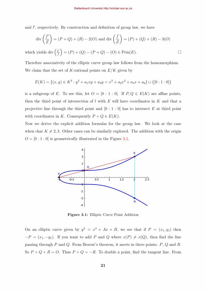
O = [0 : 1 : 0] is geometrically illustrated in the Figure 3.1.

Figure 3.1: Elliptic Curve Point Addition

On an elliptic curve given by y2 = x3 + Ax + B, we see that if P = (x1, y1) then

−P = (x1,−y1). If you want to add P and Q where x(P ) 6= x(Q), then find the line

passing through P and Q. From Bezout’s theorem, it meets in three points: P , Q and R.

So P + Q + R = O. Thus P + Q = −R. To double a point, find the tangent line. From

21


Bezout’s theorem, it meets in three points P , P and R. Thus 2P = −R.

The geometric intuition of addition can now be transformed into algebra. Let P =

(x1, y1), Q = (x2, y2) and P + Q = S = (x3, y3). Let P = (x1, y1), Q = (x2, y2) and

P + Q = S = (x3, y3), we derive some rules for obtaining x3 and y3 from A, B and the

coordinates of P and Q.

Suppose x1 6= x2. Let λ =y2 − y1

x2 − x1

. The equation of the straight line passing through P

and Q is obtained from the equationy − y1

x− x1

= λ or y = λ(x − x1) + y1. We replace the

y in y2 = x3 + Ax + B by λ(x − x1) + y1 and get 0 = x3 − (λ2)x2 + . . .. The roots of

this cubic give the x-coordinates of P , Q and −S = (x3,−y3). So x1 + x2 + x3 = λ2 and

x3 = λ2 − x1 − x2. Thus y3 = λ(x1 − x3) − y1. On the other hand, if x1 = x2 we have

two cases: the case where y1 = −y2 and the case where y1 6= −y2, in which case y1 = y2.

We have seen that the first case means P = −Q and so P +Q = O. In the second case,

P = Q. The tangent line to the elliptic curve at Q has intersection multiplicity at least 2

at P , so we use it. The equation of the tangent line is y = dydx

(x1, y1)(x− x1) + y1. Using

implicit differentiation, dydx

(x1, y1) =3x21+A

2y1. So x3 = λ2−x1−x2 and y3 = λ(x1−x3)− y1

with λ =3x21+A

2y1.

Incorporating the computations we have just made, the group law for an elliptic curve in

the form y2 = x3 + Ax+B is defined below.

In the rule below, if P is not O we let P = (x1, y1), if Q is not O we let Q = (x2, y2) and

if S = P +Q is not O we let S = (x3, y3).

i. P +O = P +O = P .

ii. We define −O = O. If P 6= O, we define −P = (x1,−y1). So if P = Q and y1 = 0,

then P +Q = O. Also for x1 = x2 and y1 6= y2, P +Q = O.

iii. If x1 6= x2 then x3 = λ2 − x1 − x2 and y3 = λ(x1 − x3)− y1 where λ =y2 − y1

x2 − x1

.

iv. If P = Q and y1 6= 0 we have x3 = λ2 − x1 − x2, y3 = λ(x1 − x3) − y1 where

λ =3x21+A

2y1.

Example 3.1.5. Let E/C be given by the equation y3 = x3 + 2x+ 1. We would like to

add the points P = (−7/16, 13/64) and Q = (0, 1).

22


We have λ = 51/28 and x1 = 0, x2 = −7/16, y1 = 1, y2 = 13/64. Then x3 = λ2−x1−x2 =

184/49 and y3 = λ(x1 − x3)− y1 = −2689/343. So P +Q = (184/49,−2689/343).

Example 3.1.6. Let α be a root of the polynomial x2 +x+ 1 ∈ F2[x] and E/F22 defined

by y2 + xy = x3 + x2 + (α + 1)x+ 1. We want to find 2(α + 1, 0). We compute

λ =dy

dx=

3x2 + 2x+ α + 1− y2y + x

=x2 + α + 1 + y

x

and at x = α + 1, we have λ = (α+1)2+α+1α+1

= 1α+1

= α. The tangent line at (α + 1, 0) is

y = αx+1. To find the value of the x-coordinate of the third point, we solve the equation

(αx+ 1)2 + x(αx+ 1) = x3 + x2 + (α + 1)x+ 1

which yields x = 0 and α + 1(twice). Hence 2(α + 1, 0) = (0, 1).

It was earlier claimed that for a smooth curve C, the local ring OP (C) is a discrete

valuation ring, we now prove the claim for elliptic curves by explicitly computing the

uniformizers. From the affine equation of an elliptic curve E : Y 2 + a3XY + a1Y =

x3 + a2x2 + a4X + a6, it is clear that K(E) = K(X)[Y ]

〈E(X,Y )〉 is a quadratic extension of K(X).

We also note that f ∈ K(E) can be written as f = w1 + w2Y for some w1, w2 ∈ K(X).

We define X = X and Y = −Y − a1X − a3. We define the norm N : K(E)→ K(X) by

f 7→ ff .

Let h ∈ OP (E). Then h = h1h2

where h2(P ) 6= 0. Thus h2 is a unit in OP (E). If h1(P ) 6= 0,

then h1 is also a unit and if t is a uniformizer at P , then ordP h = 0. Now we assume

that h1(P ) = 0 and let s represent the order of a function at P .

Suppose P = (x, y) is not a point of order 2. Then u = X − x is a uniformizer. We

have h1 = w1 + w2Y with w1, w2 ∈ K[X]. We can thus write h1 = (X − x)s0(w′1 + w′2Y )

where w′1 and w′2Y have no common factor in X − x, i.e w′1(x) 6= 0 or w′2(x) 6= 0. Set

h′1 = w′1 + w′2Y .

If h′1(P ) 6= 0, then h1 is a unit in the local ring, and so s = s0.

If h′1(P ) 6= 0, then h′1 is a unit and so h′1 = N(h1)(h′1)−1 = (X − x)s1h′′1(h′1)−1 with

h′′1 ∈ K[X] and h′′1(x) 6= 0. So s = s0 + s1.

Suppose that h′1(P ) = h′1(P ) = 0. Then (v, t) = (w′1(x), w′2(x)) is a solution to following

23


system of equations 1 Y (P )

1 Y (P )

vt

=

0

0

.

Since P is not a point of order 2, we have Y (P ) 6= Y (P ) so that the system above has

only the trivial solution. But this is a contradiction as we cannot have both w′1(x) = 0

and w′2(x) = 0.

Suppose P is a point of order 2 and char K 6= 2. We can apply an admissible change of

variables and put the curve in the form E : Y 2 = X3 + a2X2 + a4X + a6 and P = (r1, 0).

We claim that Y is a uniformizer at P .

Clearly X − r1 = (X−r1)(X−r2)(X−r3)(X−r2)(X−r3)

where r2 and r3 are the two other roots of the

polynomial X3 + a2X2 + a4X + a6. So we have X − r1 = Y 2

(X−r2)(X−r3). Note that

(X − r2)(X − r3) is a unit in OP (E). Now

h1(P ) = 0⇒ h1 = (X − r1)s2f =Y 2s2

(X − r2)s2(X − r3)s2f

for some f ∈ K[E]. Now f = w + uY where w, u ∈ K[X] and w(r1) 6= 0 or u(r1) 6= 0.

If f(P ) 6= 0, then s = 2s2. Otherwise, we must have w(r1) = 0 and u(r1) 6= 0. Thus

w(x) = (X − r1)u1 with u1 ∈ K[X] so that

f = (X − r1)u1 + uY =(X − r1)(X − r2)(X − r3)u1 + u(X − r2)(X − r3)Y

(X − r2)(X − r3)

= Yu1Y + u(X − r2)(X − r3)

(X − r2)(X − r3).

Hence s = 2s2 + 1

Finally suppose that P = (x, y) has order 2 and char K = 2. We know that y = Y (P ) =

−y − a1x− a3. There are two possible situations:

Consider E : Y 2 + XY = X3 + a2X2 + a6. Then ∆ = a6 6= 0 (j 6= 0) and a1 = 1. From

the equation y = −y − a1x − a3, we obtain 2y = x = 0 ⇒ P = (0, y) with y2 = a6. A

uniformizing parameter is given by Y + y. As it was in the previous case, we have

X = (Y + y)2 X

(Y + y)2= (Y + y)2 X

(Y 2 + a6)

which is equal to

(Y + y)2 X

X3 + a2X2 +XY= (Y + y)2 1

X2 + a2X + Y.

24


Note that X2 + a2X + Y is a unit in the local ring. Thus we can write h1 = Xs3f

where f = w + u(Y + y) for some w, u ∈ K[X] and not both w(0) and u(0) are zero.

So h1 = (Y + y)2s3 1(X2+a2X+Y )s3

f . If f(P ) 6= 0, we are done and s = 2s3. Otherwise,

w(0) = 0, so w(x) = Xw2 and u(0) 6= 0. Hence

f = Xw2 + u(Y + y) =(Y + y)2w2

X2 + a2X + Y+ u(Y + y)

= (Y + y)(Y + y)w2 + u(X2 + a2X + Y )

X2 + a2X + Y

in which case s = 2s3 + 1.

The above computations are relevant when P is finite. When P is not finite, i.e P = O,

we would like to find a uniformizer there. Recall the equation in projective coordinates

E : Y 2Z + a1XY Z + a3Y Z2 = X3 + a2X

2Z + a4X2Z + a6Z

3.

We claim that a uniformizer at O is given by u = XY. Dehomogenizing E with respect to

Y gives E ′ : Z + a1XZ + a3Z2 = X3 + a2X

2Z + a4XZ2 + a6Z

3. Since homogenisation

and dehomogenization are inverse field isomorphisms, we need to show that u′ = X is a

uniformizer at (0, 0). Notice that

Z =ZX3

X3=

ZX3

Z + a1XZ + a3Z2 − a2X2Z − a4XZ2 − a6Z3

= X3 1

1 + a1X + a3Z − a2X2 − a4XZ − a6Z2.

Note that 11+a1X+a3Z−a2X2−a4XZ−a6Z2 is a unit in the local ring at (0, 0). For any poly-

nomial f ∈ K[E], we have f = p(Z) + q(Z)X + w(Z)X2 where p, q, w ∈ K[Z]. We can

further write f = p1(Z)Zi + q1(Z)XZj + w1(Z)X2Zk where each one of p1, q1 and w1 is

either zero or not divisible by Z. When Z is replaced by X3

1+a1X+a3Z−a2X2−a4XZ−a6Z2 , we

find that

f = p2(X,Z)X3i + q2(X,Z)X3j+1 + w2(X,Z)X3k+2

where p2, q2 and w2 are regular rational functions and are; either the zero polynomial or

not zero at (0, 0). Let s = min3i, 3j + 1, 3k + 2. Then f = X sf1 where f1 is regular

and not zero at (0, 0), and so s = s. We conclude that XY

is a uniformizer at O.

3.2 Isogenies and the torsion structure

Unless otherwise stated, E denotes an elliptic curve and O its zero point.

25


Definition 3.2.1. Let E1 and E2 be elliptic curves with O1 and O2 as zero points,

respectively. A morphism ψ : E1 → E2 is called an isogeny if ψ(O1) = O2. The set of

isogenies from E onto itself is denoted End(E). Addition and multiplication in End(E)

are given by

(ψ + φ)(P ) = ψ(P ) + φ(P ) and (ψφ)(P ) = ψ(φ(P )), respectively.

One sees that End(E) is a ring. We call this ring the endomorphism ring of E. Given

E/K, we denote EndK(E) those endomorphisms defined over K. Let m ∈ Z.

The multiplication by m map [m] is defined by

[m]P =

P + P + . . .+ P︸︷︷︸

m times

if m > 0

−P − P − . . .− P︸︷︷︸−m times

if m < 0.

The map [m] is an endomorphism since it can be given by rational functions obtainable

via group law formulas and [m](O) = m(O) = O. Note that [m] is not zero for m 6= 0.

We also define deg [0] = 0.

We say that an elliptic curve E has complex multiplication (CM) if End(E) is strictly

greater than Z. For instance, all elliptic curves defined over finite fields are CM curves

and the Frobenius morphism provides an extra endomorphism.

Proposition 3.2.2. An isogeny ψ : E → E ′ is a group homomorphism, i.e. ψ(P +Q) =

ψ(P ) + ψ(Q).

Proof. Let κ1 : E → Cl0(E) and κ2 : E ′ → Cl0(E ′) be the maps P 7→ [(P ) − (O)] and

P 7→ [(P ) − (O′)]. As already shown, these maps are isomorphisms of groups. We also

know that the map ψ∗ : Cl0(E) → Cl0(E ′) is a homomorphism (from Definition 2.3.3

where we restrict to degree zero divisor classes). Since (ψ∗ κ1)(P ) = ψ∗([(P )− (O)]) =

[(ψ(P ))− (O′)] = κ2(ψ(P )) = (κ2 ψ)(P ), the following diagram commutes

E∼=κ1

- Cl0(E)

E ′

ψ

? ∼=κ2

- Cl0(E ′)

ψ∗

?

26


So ψ = κ−12 ψ∗ κ1 ⇒ ψ is a group homomorphism.

On an elliptic curve, we will denote the translation-by-Q map by τQ, i.e τQ(P ) = P +Q.

Note that this is a rational map.

Lemma 3.2.3. Let Q be a point on E. Then τQ is unramified.

Proof. Let id denote the identity map. Obviously τ−Q is the inverse of τQ. Let P ∈ E. So

eτQτ−Q(P ) = eid(P ) = 1. But by Proposition 2.2.7, eτ−QτQ(P ) = eτQ(P )eτ−Q(τQ(P )) =

eτQ(P )eτ−Q(P +Q) so that eτQ(P )eτ−Q(P +Q) = 1⇒ eτQ(P ) = 1.

Proposition 3.2.4. Let φ ∈ End(E). Then eφ(P ) is the same for all P ∈ E.

Proof. Fix a point P ∈ E. Let Q ∈ E. Then φ (τP (Q)) = φ(Q + P ) = φ(Q) + φ(P ) =

τφ(P )(φ(Q)). So we have φ τP = τφ(P ) φ.

By Proposition 2.2.7, we know that eφτP (O) = eτP (O)eφ(τP (O)) = eτP (O)eφ(P ) which

implies eφ(P ) =eφτP (O)

eτP (O). By Lemma 3.2.3, eτP (O) = 1 so that eφ(P ) = eφτP (O) ⇒

eφ(P ) = eτφ(P )φ(O) = eφ(O)eτφ(P )(O) = eφ(O). Since P was chosen arbitrarily, the result

holds.

Set eφ := eφ(P ) where P is any point on E. Then we note that for any φ, ψ ∈ End(E),

we have

eφψ(P ) = eψ(P )eφ(ψ(P )) = eψ(P )eφ(P ),

i.e eφψ = eφeψ.

Example 3.2.5. Let K = Fq and ψ be the qth-power Frobenius map. Then ψ(O) = O.

Recall that XY

is a uniformizer at O. So ordP(XY ψ)

= ordP((

XY

)q)= q, i.e eψ = q.

Thus ψ is ramified.

By Proposition 2.2.8, we have degψ =∑

P∈ψ−1(Q) eψ(P ) for any Q ∈ E and ψ ∈ End(E).

Take Q = O, then we have proved the following proposition

Proposition 3.2.6. Let ψ be an isogeny of an elliptic curve. Then

degψ = eψ|kerψ|.

Theorem 3.2.7. Let φ ∈ End(E).

27


a. For all Q ∈ E, |φ−1(Q)| = degs φ. Furthermore, degi φ = eφ.

b. If φ is unramified, then |kerφ| = degφ.

c. kerφ→ Aut(K(E)/φ∗K(E)) via the map P 7→ τ ∗P is an isomorphism of groups.

Proof. a) From Proposition 2.2.8, we know that |φ−1(Q)| = degs(φ) for almost all Q ∈ E.

For any P, P ′, choose R ∈ E such that φ(R) = P ′−P . Then there is a 1-1 correspondence

between the sets φ−1(P ) and φ−1(P ′). We claim that S 7→ S +R give one such bijection.

This is because if S + R = S ′ + R, then S = S ′. On the other hand, given Q ∈

φ−1(P ′), then φ(Q) = P ′ = φ(R) + P ⇒ Q − R ∈ φ−1(P ). This verifies that the map

is bijective. So |φ−1(Q)| is independent of Q and the first part follows. Recall that

degφ = (degi φ)(degs φ). Set Q = O in (a) so that |kerφ| = degs φ. By Proposition 3.2.6,

the other part follows.

b) Use the fact that eφ = 1 and Proposition 3.2.6.

c) For P ∈ kerφ and any f ∈ K(E), we have

τ ∗P (φ∗(f)) = (τ ∗P φ∗)(f) = (φ τP )∗(f) = φ∗(f),

i.e τ ∗P ∈ Aut(K(E)/φ∗K(E)). Thus the map is well defined. Since

τ ∗P+Q = (τP τQ)∗ = (τQ τP )∗ = τ ∗P τ ∗Q,

we note that the map is a homomorphism. Since |Aut(K(E)/φ∗K(E))| ≤ degs φ, the

proof will be complete if we show that the map is injective. Let τ ∗P (f) = f for all

f ∈ K(E). So f(P +T ) = f(T ) for all T ∈ E and f ∈ K(E). In particular, f(P ) = f(O)

for all f ∈ K(E) so that P = O.

For φ ∈ End(E), recall that φ∗ on K(E) is given as f 7→ f φ. On the divisor group, we

define φ∗ : Div(E)→ Div(E) by (Q) 7→∑

P∈φ−1(Q) eφ(P )(P ) which Z-linearly extends to

the whole divisor. The following proposition provides a method for computing divisors

of composition of functions.

28


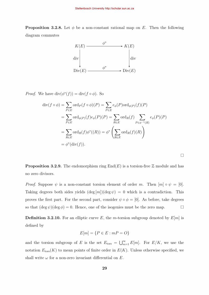
Proposition 3.2.8. Let φ be a non-constant rational map on E. Then the following

diagram commutes

K(E)φ∗

- K(E)

Div(E)

div

? φ∗- Div(E)

div

?

Proof. We have div(φ∗(f)) = div(f φ). So

div(f φ) =∑P∈E

ordP (f φ)(P ) =∑P∈E

eφ(P )ordφ(P )(f)(P )

=∑P∈E

ordφ(P )(f)eφ(P )(P ) =∑R∈E

ordR(f)∑

P∈φ−1(R)

eφ(P )(P )

=∑R∈E

ordR(f)φ∗((R)) = φ∗

(∑R∈E

ordR(f)(R)

)= φ∗(div(f)).

Proposition 3.2.9. The endomorphism ring End(E) is a torsion-free Z module and has

no zero divisors.

Proof. Suppose ψ is a non-constant torsion element of order m. Then [m] ψ = [0].

Taking degrees both sides yields (deg [m])(degψ) = 0 which is a contradiction. This

proves the first part. For the second part, consider ψ φ = [0]. As before, take degrees

so that (degψ)(degφ) = 0. Hence, one of the isogenies must be the zero map.

Definition 3.2.10. For an elliptic curve E, the m-torsion subgroup denoted by E[m] is

defined by

E[m] = P ∈ E : mP = O

and the torsion subgroup of E is the set Etors =⋃∞m=1 E[m]. For E/K, we use the

notation Etors(K) to mean points of finite order in E(K). Unless otherwise specified, we

shall write ω for a non-zero invariant differential on E.

29


Theorem 3.2.11. Let ψ, φ : E → E ′ be isogenies. Then (ψ + φ)∗ω = ψ∗ω + φ∗ω.

Proof. See [8].

Corollary 3.2.12. For m ∈ Z, we have [m]∗ω = mω

Proof. Clearly form = 0 andm = 1, the result holds. Form = −1, note that [−1](x, y) =

(x,−y − a1x− a3) so that

[−1]∗ω = [−1]∗(

dx

2y + a1x+ a3

)=

dx

2(−y − a1x− a3) + a1x+ a3

= − dx

2y + a1x+ a3

.

Since [m+ 1]∗ω = [m]∗ω+ [1]∗ω by Theorem 3.2.11, the rest proceeds by induction on m

(downwards and upwards).

Corollary 3.2.13. A non-constant multiplication-by-m map [m] on E is separable.

Proof. We note that [m]∗ω = mω 6= 0 which means that [m] is separable by Proposition

2.3.7 (c).

Corollary 3.2.14. Let E be defined over a finite field Fq with characteristic p. Let ψ :

E → E be the qth-power Frobenius morphism. For m,n ∈ Z, the map [m]+[n]ψ : E → E

is inseparable if and only if p|m.

Proof. By Example 3.2.5, we know that ψ is ramified therefore inseparable. So ([m] +

[n] ψ)∗ω = mω = 0 if and only if p|m.

We will use the following proposition to show that for an elliptic curve defined over a

characteristic zero field, its endomorphism ring is commutative.

Proposition 3.2.15. Let E/K be an elliptic curve and φ ∈ End(E). Then div(φ∗ω) =

φ∗div(ω) and div(ω) = 0.

Proof. See [8].

Theorem 3.2.16. Consider an elliptic curve E/K. Let ν : End(E) → K be defined by

φ 7→ cφ where φ∗ω = cφω. Then

a. ν is a homomorphism of rings.

b. ker ν consists of inseparable endomorphisms.

30


Proof. a) Recall that dimK(E)ΩE = 1 ⇒ φ∗ω = cφω for some cφ ∈ K(E). Furthermore,

we have

div(φ∗ω) = div(cφω) = div(cφ) + div(ω) = div(cφ) = 0.

This follows from Proposition 3.2.15. Thus div(cφ) = 0 implies that cφ has no poles or

zeros, hence cφ ∈ K. So ν is well defined. By Theorem 3.2.11, it follows that

cφ+ψω = (φ+ ψ)∗ω = φ∗ω + ψ∗ω = cφω + cψω

so that ν(φ+ ψ) = ν(φ) + ν(ψ).

b) We know that cφ = 0 is the same as φ∗ω = 0 which is the same as saying φ is

inseparable.

Consequently, if char K = 0, then every non-constant endomorphism is separable, and

so End(E) → K which implies that End(E) is commutative. This result will be helpful

in the characterisation of End(E).

Let ψ : E → E ′ be a non-constant isogeny of degree m. There is a unique isogeny

denoted ψ : E ′ → E satisfying ψ ψ = [m], see [8]. Now suppose that ψ1 ψ = ψ2 ψ.

Then (ψ1 − ψ2) ψ = [0]. Since ψ is non-constant, it follows that ψ1 = ψ2. We call ψ,

the dual isogeny. If ψ = [0], we set ψ = [0].

Theorem 3.2.17. With the notation above, we have the following

a. ψ ψ = [m]E′ where [m]E′ denotes [m] on E ′.

b. Let λ : E ′ → E ′′ be another isogeny with degλ = n. Then λ ψ = ψ λ.

c. If φ is another isogeny from E to E ′, then ψ + φ = ψ + φ.

d. For all m ∈ Z, [m] = [m] and deg [m] = m2.

e. deg ψ = degψ.

f. ψ = ψ.

31


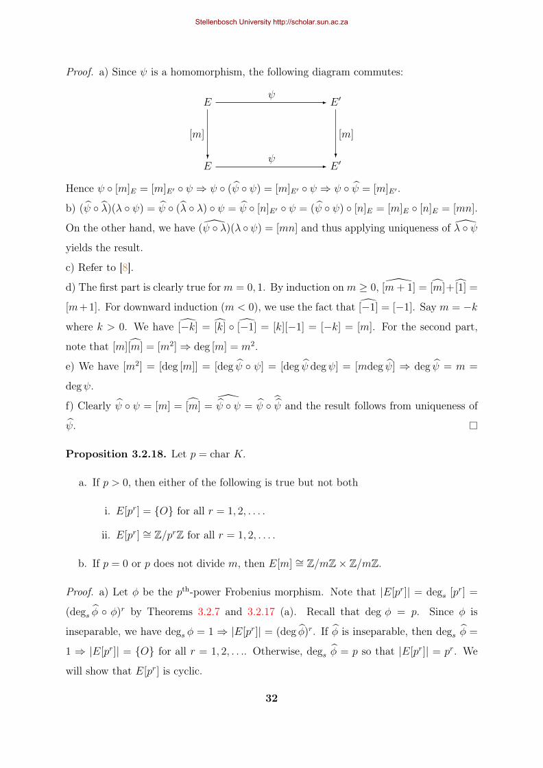
Proof. a) Since ψ is a homomorphism, the following diagram commutes:

Eψ

- E ′

E

[m]

? ψ- E ′

[m]

?

Hence ψ [m]E = [m]E′ ψ ⇒ ψ (ψ ψ) = [m]E′ ψ ⇒ ψ ψ = [m]E′ .

b) (ψ λ)(λ ψ) = ψ (λ λ) ψ = ψ [n]E′ ψ = (ψ ψ) [n]E = [m]E [n]E = [mn].

On the other hand, we have (ψ λ)(λ ψ) = [mn] and thus applying uniqueness of λ ψ

yields the result.

c) Refer to [8].

d) The first part is clearly true form = 0, 1. By induction onm ≥ 0, [m+ 1] = [m]+[1] =

[m+1]. For downward induction (m < 0), we use the fact that [−1] = [−1]. Say m = −k

where k > 0. We have [−k] = [k] [−1] = [k][−1] = [−k] = [m]. For the second part,

note that [m][m] = [m2]⇒ deg [m] = m2.

e) We have [m2] = [deg [m]] = [deg ψ ψ] = [deg ψ degψ] = [mdeg ψ] ⇒ deg ψ = m =

degψ.

f) Clearly ψ ψ = [m] = [m] =ψ ψ = ψ ψ and the result follows from uniqueness of

ψ.

Proposition 3.2.18. Let p = char K.

a. If p > 0, then either of the following is true but not both

i. E[pr] = O for all r = 1, 2, . . . .

ii. E[pr] ∼= Z/prZ for all r = 1, 2, . . . .

b. If p = 0 or p does not divide m, then E[m] ∼= Z/mZ× Z/mZ.

Proof. a) Let φ be the pth-power Frobenius morphism. Note that |E[pr]| = degs [pr] =

(degs φ φ)r by Theorems 3.2.7 and 3.2.17 (a). Recall that deg φ = p. Since φ is

inseparable, we have degs φ = 1 ⇒ |E[pr]| = (deg φ)r. If φ is inseparable, then degs φ =

1 ⇒ |E[pr]| = O for all r = 1, 2, . . .. Otherwise, degs φ = p so that |E[pr]| = pr. We

will show that E[pr] is cyclic.

32


For r = 1, clearly E[p] ∼= Z/pZ. Assume by induction that E[pr−1] ∼= Z/pr−1Z. Define

η : E[pr] → E[pr−1] by P 7→ pP . We note that η is the restriction of the surjective map

[p] on E[pr]. Clearly, the preimage of a pr−1-torsion point under [p] is a pr-torsion point.

Hence η is a surjective homomorphism. By the induction hypothesis, there is Q ∈ E[pr−1]

which has order pr−1. So there is P ∈ E[pr] such that pP = Q. But pr−1Q = O and

piQ 6= O for all 1 ≤ i ≤ r − 2 implies that P has order pr.

b) We know that |E[m]| = m2. Suppose m is prime. Then by the fundamental theorem

on finite abelian groups, E[m] ∼= Z/mZ × Z/mZ or E[m] ∼= Z/m2Z. But the later case

means that E[m] contains a point of orderm2 which is not annihilated upon multiplication

by m, a contradiction.

Suppose m is not prime, then m = m′q with q a prime. We then have

E[m′] = P : m′P = O

= qP : m′qP = O since [q] is surjective

= qP : mP = O = qE[m].

Again by the fundamental theorem, we have

E[m] ∼= Z/n1Z× Z/n2Z× . . .× Z/nrZ

with unique n1, n2, . . . , nr ≥ 2 such that ni|ni+1. Hence E[m′] ∼= qZ/n1Z × qZ/n2Z ×

. . .× qZ/nrZ ∼= Z/s1Z× Z/s2Z× . . .× Z/srZ where

si =

ni if q does not divide ni

niq

if q divides ni

and si divides si+1 since ni|ni+1. By induction hypothesis to m′, i.e E[m′] ∼= Z/m′Z ×

Z/m′Z and the fact that si’s are unique, we have s1 = s2 = . . . = sr−2 = 1 and sr−1 =

sr = m′. Hence n1 = n2 = . . . = nr−2 = q and nr−1 = nr = qm′ = m. So |E[m]| = m2 =

qr−2m2 ⇒ r = 2.

Lemma 3.2.19. Let m,n ∈ Z and (m,n) = 1. Then E[mn] ∼= E[m]× E[n].

33


Proof. There are integers x1 and x2 such that x1n + x2m = 1. Define maps π : E[m] ×

E[n]→ E[mn] by (P,Q) 7→ P +Q and π′ : E[mn]→ E[m]×E[n] by P 7→ (x1nP, x2mP ).

It is not difficult to see that the two maps are inverse group isomorphisms.

Theorem 3.2.20. With the notation introduced in Proposition 3.2.18, if p divides m,

then

E[m] ∼= Z/m′Z× Z/m′Z or E[m] ∼= Z/mZ× Z/m′Z

where m = pnm′ with (m′, p) = 1.

Proof. By Lemma 3.2.19, E[m] ∼= E[m′] × E[pn]. If E[p] = O, then E[pn] = O by

Proposition 3.2.18(a). So E[m] ∼= Z/m′Z×Zm′/Z. On the other hand, if E[pn] = Z/pnZ,

then E[m] ∼= E[m′]×Z/pnZ ∼= Z/m′Z×Z/m′Z×Z/pnZ. Since Z/m′Z×Z/pnZ ∼= Z/mZ

by Chinese Remainder Theorem, we have E[m] ∼= Z/m′Z× Z/mZ.

We call an elliptic curve in finite characteristic p ordinary if E[p] ∼= Z/pZ and supersin-

gular if E[p] ∼= 0.

3.3 Weil pairing and elliptic curves over finite fields

The Weil pairing will be indirectly important in computing the cardinality of torsion

points on elliptic curves defined over finite fields. We exhibit its construction and deduce

its properties.

Assume E is defined over K and (charK,m) = 1. Let T ∈ E[m]. The divisor m(T ) −

m(O) is principal by Proposition 3.1.3. So there is f ∈ K(E)× such that div(f) = m(T )−

m(O). Let T ′ ∈ E[m2] be chosen such that mT ′ = T . Then the divisor∑

S∈E[m](T′ +

S)−(S) is principal since∑

S∈E[m] T′+S−S = m2T ′ = O and the degree of the divisor is

0. So we can find a function g such that div(g) =∑

S∈E[m](T′+S)− (S). Let T = T ′+S

in the summation. Clearly T = T ′ + S ⇔ mT = mT ′ + mS = T . Hence we can restate

the divisor of g as

div(g) =∑mT=T

(T )−∑mS=O

(S).

34


We want to compute div(f m). We know that [m] is separable and e[m](P ) = 1 for all

P ∈ E. By definition, we have

div(f m) = [m]∗ (div(f)) = m∑

P∈[m]−1(T )

e[m](P )(P )−m∑

Q∈[m]−1(O)

e[m](Q)(Q)

= m∑mP=T

(P )−m∑mQ=O

(Q)

= div(gm).

It follows that fg = kgm for some k ∈ K. Without loss of generality, assume k = 1. Then

for S ∈ E[m] and P ∈ E, we have g(P+S)m = f(m(P+S)) = f(mP ) = g(P )m ⇒ g(P+S)g(P )

is an mth root of unity. Let µm = x ∈ K : xm = 1.

Definition 3.3.1. The mth Weil pairing is the map em : E[m]× E[m]→ µm defined by

em(S, T ) =g(P + S)

g(P )

where P is any point on E such that g(P + S) and g(P ) are defined and nonzero.

Maintaining our assumption on m, we have the following theorem.

Theorem 3.3.2. The map em satisfies the following properties

a. Bilinearity in each variable, i.e em(S1 +S2, T ) = em(S1, T )em(S2, T ) and em(S, T1 +

T2) = em(S, T1)em(S, T2) for all S, T, S1, S2, T1, T2 ∈ E[m].

b. em(T, T ) = 1 for all T ∈ E[m] and so em(S, T ) = em(T, S)−1 for all S, T ∈ E[m].

c. Nondegeneracy in both variables, i.e em(S, T ) = 1 for all T ∈ E[m] ⇒ S = O and

em(S, T ) = 1 for all S ∈ E[m]⇒ T = O.

d. em(σS, σT ) = σem(S, T ) for all σ ∈ Gal(K/K).

e. em(α(S), α(T )) = em(S, T )degα for all endomorphisms α.

Proof. (a) em(S1 + S2, T ) = g(P+S1+S2)g(P )

= g(P+S1+S2)g(P+S1)

g(P+S1)g(P )

= em(S2, T )em(S1, T ). For

the second part, let T3 = T1 + T2. Then there is g ∈ K(E)× such that

div(g) = (T1) + (T2)− (T3)− (O).

35


Let fi, gi be the functions used to define em(S, Ti). Thus div(fi) = m(Ti) −m(O)

and gmi = fi m. We have

div(

f3

f1f2

)= div(f3)− div(f1)− div(f3)

= m(T3)−m(O)−m(T2) +m(O)−m(T1) +m(O)

= m(div(g)) = div(gm)

implying that f3f1f2

= bgm for some b ∈ K× ⇒ f3 = bf1f2gm. Composing with m, we

get f3m = b(f1m)(f2m)(gmm)⇒ gm3 = bgm1 gm2 (gm)m ⇒ g3 = b1/mg1g2(gm)

so that

em(S, T1 + T2) =g3(P + S)

g3(P )=g1(P + S)

g1(P )

g2(P + S)

g2(P )

g(mP +O)

g(mP )

= em(S, T1)em(S, T2)

(b) Recall the translation by Q map written τQ. Now for j ∈ Z≥0, we note the following

div(f τjT ) = τ ∗jT (div(f))

= m∑

P∈τ−1jT (T )

(P )−m∑

Q∈τ−1jT (O)

(O) since eτjT (P ) = 1 for all P ∈ E

= m(T − jT )−m(−jT )

which implies

divm−1∏j=0

f τjT =m−1∑j=0

m(T − jT )−m(−jT ) = 0,

and so∏m−1

j=0 f τjT ∈ K. Recall that mT ′ = T . We deduce that(div

m−1∏j=0

g τjT ′)m

= divm−1∏j=0

gm τjT ′

= divm−1∏j=0

f [m] τjT ′

= divm−1∏j=0

f τjT [m].

The last statement follows from the fact that

[m] τjT ′(P ) = m(P + jT ′) = mP + jmT ′

36


which is equal to

mP + jT = ([m] τjT )(P ) = (τjT [m])(P ).

Clearly∏m−1

j=0 f τjT [m] is constant and so∏m−1

j=0 g τjT ′ is constant. Hence at P

and P + T ′, the product takes the same value, i.e

m−1∏j=0

g τjT ′(P ) =m−1∏j=0

g τjT ′(P + T ′)

which implies that

g(P ) = g(P +mT ′) = g(P + T )⇒ g(P + T )

g(P )= em(T, T ) = 1.

Using bilinearity, we have

em(S + T, S + T ) = em(S, T )em(T, S)em(S, S)em(T, T )

which implies that em(S, T ) = em(T, S)−1.

(c.) Let T ∈ E[m] such that em(S, T ) = 1 for all S ∈ E[m]. Then g(S + P ) = g(P ) for

all S ∈ E[m]. In other words, (g τS) = τ ∗S(g) = g for all S ∈ E[m]. By Theorem

3.2.7, we have g ∈ Aut(K(E)/[m]∗K(E)) which implies that g = f [m] for some

f ∈ K(E). Now

fm [m] = gm = f [m]⇒ f = fm

since [m] is a non-constant map. We have

mdiv(f) = div(f) = m(T )−m(O)⇒ div(f) = (T )− (O)

so that T = O by Proposition 2.3.13. On the other hand, if S ∈ E[m] such that

em(S, T ) = 1 for all T ∈ E[m], then em(T, S) = 1 for all T ⇒ S = O.

(d.) Consider the functions f and g in our construction. Then

div(fσ) = m(σ(T ))−m(σ(O)) = m(σ(T ))−m(O)

and

σ(em(S, T )) =gσ(σ(P ) + σ(T ))

gσ(σ(P ))= em(σ(S), σ(T )).

37


(e.) Let α be a separable endomorphism and kerα = B1, B2, . . . , Bs. Thus deg α =

s. Let div(fT ) = m(T ) − m(O) and div(fα(T )) = m(α(T )) − m(O) and we have

fT [m] = gmT and fα(T ) [m] = gmα(T ). Let τB be the translation by B. We note that

div(fT τ−Bi) = τ ∗−Bi(div(fT )) = m(T +Bi)−m(Bi)

and

div(fα(T ) α) = m∑

Q∈α−1(α(T ))

(Q)−m∑

R∈α−1(O)

(R)

= m∑

α(Q)=α(T )

(Q)−m∑

α(R)=O

(R)

= m

(∑i

(T +Bi)−m(Bi)

)

= div

(∏i

fT τ−Bi

).

Applying the same trick as before, for every i, choose B′i such that mB′i = Bi. Then

a calculation shows that gT (P −B′i)m = fT (mP −Bi) and hence

div

(∏i

(gT τ−B′i)m

)= div

∏i

fT [m] τ−Bi

= div∏i

fT τ−Bi [m]

= [m]∗div

(∏i

fT τ−Bi

)= [m]∗div(fα(T ) α)

= div(fα(T ) α [m])

= div(gmα(T ) α)

= div(gα(T ) α)m

which implies that ∏i

(gT τ−B′i) = cgα(T ) α for some c ∈ K. (3.3.1)

38


So we have

em(α(S), α(T )) =gα(T )(α(P ) + α(S))

gα(T )α(P )

=(gα(T ) α)(P + S)

(gα(T ) α)(P )

=

∏i gT (P −B′i + S)

gT (P −B′i)by Equation 3.3.1

=∏i

em(S, T ) by definition of em

= em(S, T )degα.

For α inseparable, refer to [10].

From E[m] ∼= Z/mZ × Z/mZ, we note that E[m] is a Z/mZ-module of rank 2. So we

can find 2 linearly independent generators T1 and T2 for E[m]. For an endomorphism α,

we have α(T1) = aT1 + cT2 and α(T2) = bT1 + dT2 for some a, b, c, d ∈ Z/mZ. We define

αm to be the matrix

αm =

a b

c d

.

Corollary 3.3.3. Let T1, T2 be a basis for E[m]. Then em(T1, T2) is a primitive mth

root of unity.

Proof. Let γ = em(T1, T2) with γn = 1. Then by bilinearity, we have em(T1, nT2) = 1

and em(T2, nT2) = 1. Let P ∈ E[m]. Then P = aT1 + bT2 for some a, b ∈ Z. So

em(P, nT2) = em(aT1 +bT2, nT2) = em(T1, nT2)aem(T2, nT2)b = em(T1, T2)anem(T2, T2)nb =

1, i.e em(P, nT2) = 1 for all P ∈ E[m]⇒ nT2 = O ⇔ m|n⇒ γ is a primitive mth root of

unity.

Corollary 3.3.4. If E[m] ⊆ E(K), then µm ∈ K.

Proof. As before, let T1, T2 be a basis for E[m]. By assumption, σ(Ti) = Ti for all

σ ∈ Gal(K/K) and i = 1, 2. Now γ = em(σ(T1), σ(T2))) = σ(em(T1, T2)) = σ(γ) so that

γ ∈ K. By Corollary 3.3.3, γ generates µm and so µm ⊂ K.

39


One of the applications of Corollary 3.3.4 is that E[m] * E(Q) for all m ≥ 3. To see

this, assume that E[m] ⊆ E(Q) for some m ≥ 3 then µm ∈ Q, which is a contradiction.

Proposition 3.3.5. Let E be defined over K and α ∈ End(E). Assume (charK,m) = 1.

Then

detαm ≡ degα (mod m).

Proof. Maintaining the notation in Corollary 3.3.3, we note that γdegα = em(T1, T2)degα =

em(α(T1), α(T2)) = em(aT1 + cT2, bT1 + dT2) = em(T1, T2)ad−bc = γdetαm , and the result

follows.

Proposition 3.3.6. Let α be a non-zero endomorphism. Then α2− [1+degα−deg ([1]−

α)]α + degα = [0].

Proof. Let f = α2−[1+degα−deg ([1]−α)]α+degα. Restricting all the endomorphisms

to E[m] for (m, charK) = 1, we have fm = α2m− [1 + detαm− det (I−αm)]αm + detαm.

Clearly Trαm = 1 + detαm − det (I− αm), and so by Cayley-Hamilton theorem, fm = 0.

Varying m, we note that f(P ) = O for infinitely many torsion points P . It follows that

f(P ) = O for all P on E, otherwise we would have f = (ψ, φ) where φ or ψ has infinitely

many poles, which is a contradiction.

3.3.7 Elliptic curves over a finite field

In this section we look at elliptic curves over Fq with characteristic p > 0. One of the

tasks is to derive a formula for computing the number of points on an elliptic curve with

coordinates in higher extensions of Fq. We first begin with an estimate on the number of

points on E(Fq).

3.3.8 Hasse’s Theorem

Definition 3.3.9. Let G be an abelian group. A function q : G → R is called positive

definite quadratic form if it satisfies the following

a. q(−a) = q(a) ∀ a ∈ G.

b. q(a) ≥ 0 ∀ a ∈ G.

40


c. q(a) = 0 if and only if a = 0.

d. The map (a, b) 7→ q(a+ b)− q(a)− q(b) is bilinear.

Lemma 3.3.10. The degree map deg : Hom(E,E ′)→ Z is a positive definite quadratic

form.

Proof. a) Note that −φ = [−1]E′ φ⇒ deg (−φ) = deg [−1]E′ degφ = deg φ

b) Let 〈φ, ψ〉 = deg (φ+ ψ)− deg φ− deg ψ. Then

[〈φ, ψ〉]E = [deg (φ+ ψ)]E − [deg φ]E − [deg ψ]E

= (φ+ ψ) (φ+ ψ)− φ φ− ψ ψ

= (φ+ ψ) (φ+ ψ)− φ φ− ψ ψ

= φ ψ + ψ φ.

From this, it follows that for all φ1, φ2 ∈ Hom(E,E ′),

[〈φ1 + φ2, ψ〉]E = [〈φ1, ψ〉]E + [〈φ2, ψ〉]E = [〈φ1, ψ〉+ 〈φ2, ψ〉]E.

As Z injects into End(E), we must have 〈φ1 +φ2, ψ〉 = 〈φ1, ψ〉+ 〈φ2, ψ〉. Linearity in the

second variable holds in a similar way.

(c) Clear since deg φ > 0 for φ non-constant.

Lemma 3.3.11. Let G be an abelian group and q : G → R a positive definite quadratic

form. Then

|q(ψ − φ)− q(ψ)− q(φ)| ≤ 2√q(φ)q(ψ) forall ψ, φ ∈ G

Proof. Let 〈φ, ψ〉 = q(ψ+φ)−q(ψ)−q(φ). Then 〈−φ, φ〉 = q(0)−q(−φ)−q(φ) = −2q(φ)

for all φ ∈ G. Note that 〈−mφ,mφ〉 = m2〈−φ, φ〉, using bilinearity. Thus 〈−mφ,mφ〉 =

−2m2q(φ) for all m ∈ Z. On the other hand, 〈−mφ,mφ〉 = −2q(mφ) by definition.

Hence q(mφ) = m2q(φ) for all m ∈ Z.

If ψ = 0, the inequality holds. So we assume that ψ 6= 0. Then

q(mψ − nφ) = 〈mψ,−nφ〉+ q(mψ) + q(nφ)

= −mn〈ψ, φ〉+m2q(ψ) + n2q(φ) for any m,n ∈ Z.

41


Setting m = 〈ψ, φ〉 and n = 2q(ψ), we get q(mψ − nφ) = −q(ψ)〈ψ, φ〉2 + 4q(ψ)2q(φ).

Since q is positive definite, we obtain the inequality, q(ψ)[4q(ψ)q(φ)− 〈ψ, φ〉2] ≥ 0. Now

ψ 6= 0 implies the result.

Since the equation of E has coefficients in Fq, it follows that the qth-power Frobenius

map is an automorphism. Let φq represent this map, then φq : E → E is defined as

(x, y) 7→ (xq, yq). Obviously, P ∈ E(Fq) if and only if φq(P ) = P i.e P ∈ ker(1− φq). By

Corollary 3.3.12, 1− φq is separable, and thus |ker(1− φq)| = deg(1− φq) = #E(Fq).

Theorem 3.3.12. (Hasse) Let E be an elliptic curve over a finite field Fq. Then

|#E(Fq)− q − 1| ≤ 2√q.

Proof. Take G = End(E) and ψ = [1] in Lemma 3.3.11 so that

|deg(1− φq)− 1− deg φq| ≤ 2√

deg φq.

Using the fact that deg φq = q, the result follows.

Theorem 3.3.13. For E/Fq, let φq be the qth-power Frobenius map and a = q + 1 −

#E(Fq). Let α, β be the roots of the polynomial X2 − aX + q. Then #E(Fqn) =

qn + 1− αn − βn for all n ≥ 1.

Proof. By Proposition 3.3.6, we must have φ2q−[1+degφq−deg ([1]−φq)]φq+degφq = [0],

i.e φ2q − [1 + q − |E(Fq)|]φq + degφq = 0 in End(E). Let a = 1 + q − |E(Fq)|. Then φq is

a zero in End(E) of the polynomial X2 − aX + q. Let L = Fqn which is a degree n finite

extension of Fq and denote the map (x, y) 7→ (xqn, yq

n) by φL. The integer s, if it exists,

such that φ2L + sφL + qn = 0 is unique since, if φ2

L + s′φL + qn = 0 for another integer

s′, then sφL − s′φL = 0 ⇒ s = s′ by surjectivity of φL. By this argument, a is the only

number satisfying the equation X2− aX + q = 0 given that φq is a zero of the associated

polynomial. Using φL = φnq and Proposition 3.3.6, we note that s = 1 + qn − |E(Fqn)|

is the unique integer such that (φnq )2 − sφnq + qn = 0, i.e φq is a root of the polynomial

X2n − sXn + qn.

Let α and β be roots of the polynomial X2 − aX + q so that a = α + β and αβ = q.

Denote the discriminant of the quadratic by D, so D = a2 − 4q. By Theorem 3.3.12,

42


D is not a positive integer. Clearly, α and β are integers in the imaginary quadratic

extension Q(√D), i.e α, β ∈ Z[θ] where θ = 1+

√D

2if D ≡ 1(mod 4) and θ =

√D,

otherwise. Since D < 0, α and β are complex conjugates, and thus αn + βn ∈ R. Hence

αn + βn ∈ Z[θ] ∩ R = Z.

Let g(X) = X2n − (αn + βn)Xn + qn. Then g(X) ∈ Z[X]. Furthermore, g(α) = 0 and

g(β) = 0 so that X2−aX+ q divides g(X) implying that φ2nq − (αn+βn)φnq + qn = 0.

The number a is called the trace of Frobenius.

Example 3.3.14. Consider E defined over F2 given by y2 + xy = x3 + x2 + 1. Then

#E(F2) = 2 so that a = 2 + 1−2 = 1. Now α = 1+√

7i2

and β = 1−√

7i2

are the roots of the

polynomial X2 −X + 2, and α6 + β6 = 9. By Theorem 3.3.13, #E(F26) = 65− 9 = 56.

3.4 Characterisation of the endomorphism ring

In this section we would like to characterise the endomorphism ring of an elliptic curve.

We do that by proving a general result that applies to certain rings. The tensor product

is always taken over Z.

Definition 3.4.1. Let H be a Q-algebra that is finitely generated over Q. An order in

H is a subring and finitely generated Z-module R satisfying R⊗Q = H. R is said to be

maximal if given that R′ is an order in H with R ⊂ R′, then R = R′.

Example 3.4.2. For a quadratic number field Q(√m) where m < 0 is square free and

4 does not divide m − 1, we note that the ring of integers Z[√m] is an order since

Z[√m]⊗Q = Q[

√m].

Remark 3.4.3. It turns out that an order in an imaginary quadratic extension of Q

can be written in the form Z + fR where f ∈ Z>0 and R is the ring of integers of the

extension. In this case we see that the ring of integers is the maximal order.

Definition 3.4.4. A definite quaternion algebra over Q is a ring of the form

H = Q + Qα + Qβ + Qαβ

where α2, β2 ∈ Q, α2 < 0, β2 < 0 and αβ = −βα.

43


Theorem 3.4.5. Let R be a characteristic 0 ring with no zero divisors. If R is a finitely

generated Z-module of rank ≤ 4 and further satisfies the following properties

a. R has an anti-involution α 7→ α with

α + β = α + β, ˆα = α, αβ = βα for all α ∈ R and α = α for all α ∈ Z.

b. For every α ∈ R, αα ∈ Z≥0 and αα = 0 if and only if α = 0.

Then R = Z or R is an order in an imaginary quadratic number field or R is an order in

a definite quaternion algebra over Q.

Proof. Consider the product H = R⊗Q. Note that an arbitrary element of H looks like∑j rj ⊗ qj where rj ∈ R and qj ∈ Q. So we extend the anti-involution on R to H by

r⊗ q 7→ r⊗ q. Thus with this extended anti-involution, Q is fixed, i.e α = α for all α ∈ Q

and αα ∈ Q≥0. We define a norm and trace (from H to Q) in the following way

Nα = αα and Tr α = α + α.

Lemma 3.4.6. The trace and the norm exhibit the following properties

a. Trα = 1 + Nα− N(α− 1)

b. Tr is Q-linear

c. If α ∈ Q, then Trα = 2α

d. If α ∈ H, α 6= 0 such that Trα = 0, then α2 < 0 and α2 ∈ Q.

Proof. a) we note that

1 + Nα− N(α− 1) = 1 + αα− (α− 1)(α− 1)

= 1 + αα− αα + α + α− 1

= Trα

This property implies that for α ∈ H,Trα ∈ Q

b) Apply the fact that α = α for all α ∈ Q.

44


c) By the definition of Tr and the fact that the anti-involution fixes Q.

d) Clearly, 0 = (α− α)(α− α) = α2 + Nα which implies that α2 = −Nα ∈ Q.

SinceR is a Z-module of rank at most 4, it is enough to show thatH = Q or an imaginary

quadratic number field or a definite quaternion algebra.

If H = Q, then R = Z. Otherwise, there exists α ∈ H such that α /∈ Q. Since

Tr(α − 12Trα) = 0, we may replace α with α − 1

2Trα and assume that Trα = 0. By

Lemma 3.4.6 (d), we have α2 < 0 and α2 ∈ Q so that we can take H = Q(α). If

H 6= Q(α), then we can find β′ ∈ H such that β′ /∈ Q(α). Let β = β′ − Trβ′2− Tr(αβ′)

2α2 α.

Then

Tr β = Tr(β′ − Tr β′

2− Tr(αβ′)

2α2α

)= Tr β′ − Tr β′ − Tr(αβ′)

2α2Trα

= 0 since Trα = 0.

Replacing β′ by β, we may assume that Tr β = 0. Furthermore, we have

αβ = αβ′ − Tr β′

2α− Tr(αβ′)

2

which leads to

Tr(αβ) = Tr(αβ′)− Tr β′

2Trα− Tr(αβ′) = 0.

Thus the conditions Trα = 0,Tr β = 0 and Tr(αβ) = 0 imply that

α = −α, β = −β and αβ = −βα

which yield

αβ = −βα.

Hence Q(α, β) = Q + Qα + Qβ + Qαβ is a definite quaternion algebra. To show that

H = Q(α, β), it suffices to show that 1, α, β, αβ are linearly independent over Q. Assume

we have a relation r + sα + tβ + uαβ = 0 where r, s, t, u ∈ Q. Then

Tr(r + sα + tβ + uαβ) = 0⇒ 2r = 0⇒ r = 0

45


so that sα+ tβ + uαβ = 0. Upon left-multiplication by α and right-multiplication by β,

we obtain

(α2s)β + (β2t)α + uα2β2 = 0

which implies that

α2s = β2t = uα2β2 = 0

as 1, α and β are linearly independent over Q. Hence s = t = u = 0, since α2, β2 6= 0.

This completes the proof.

Corollary 3.4.7. E/K be an elliptic curve. Then End(E) is either Z or an order in

an imaginary quadratic number field or an order in a definite quaternion algebra. If

char K = 0, then End(E) cannot be an order in a definite quaternion algebra.

Proof. Use Theorem 3.4.5 with R = End(E) with the anti-involution being α 7→ α where

α is the dual isogeny of α.

If char K = 0, then End(E) is commutative. We note that if αβ = −βα with α, β 6= 0

then End(E) has zero divisors.

Definition 3.4.8. If End(E) > Z, we say E is an elliptic curve with complex multipli-

cation by R where R ∼= End(E) (as rings) is an order given in Theorem 3.4.5

Example 3.4.9. The curve given by

y2 = x3 + 9x

is an elliptic curve over C with complex multiplication by Z[i].

Proof. Clearly it is an elliptic curve. We easily check that φ : (x, y) 7→ (−x, iy) provides

an extra endomorphism. By Corollary 3.4.7, End(E) is an order in an imaginary quadratic

extension ofQ. Now φ2(x, y) = (x,−y) = −(x, y) so that φ2 = [−1]. Thus Z[i] → End(E)

via a + bi 7→ [a] + [b]φ. Since by Remark 3.4.3, Z[i] is maximal in Q(i), we must have

End(E) ∼= Z[i].

46


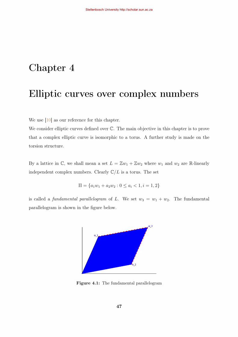
Chapter 4

Elliptic curves over complex numbers

We use [10] as our reference for this chapter.

We consider elliptic curves defined over C. The main objective in this chapter is to prove

that a complex elliptic curve is isomorphic to a torus. A further study is made on the

torsion structure.

By a lattice in C, we shall mean a set L = Zw1 + Zw2 where w1 and w2 are R-linearly

independent complex numbers. Clearly C/L is a torus. The set

Π = a1w1 + a2w2 : 0 ≤ ai < 1, i = 1, 2

is called a fundamental parallelogram of L. We set w3 = w1 + w2. The fundamental

parallelogram is shown in the figure below.

Figure 4.1: The fundamental parallelogram

47


Note that z ∈ ΠmodL for every z ∈ C. A doubly periodic meromorphic (elliptic) function

is a function f : C→ C ∪∞ such that f(z + w) = f(z) where w ∈ L. If f has no poles,

then it is constant. To see this, we use the fact that such a function can only have finitely

many poles on a compact subset, on the the closure Π = Π ∪ ∂Π for instance. The

notation ∂Π stands for the boundary of Π. Thus f is holomorphic and bounded on C.

By Liouvilles’s theorem, f is constant.

Theorem 4.0.10. Let f be an elliptic function. We have

a.∑

w∈Π Resw(f) = 0.

b. If f 6= 0, then∑

w∈Π ordw(f) = 0 and∑

w∈Π ordw(f)w ∈ L.

c. If f is non-constant then it is surjective. Let m be the sum of orders of poles of f

in Π. Then f(z) = z0 for any z0 ∈ C has m solutions (counting multiplicities).

d. If f has a single pole in Π, then it cannot be simple.

Proof. Cauchy’s theorem states that∑w∈Π

Resw(f) =1

2πi

∫∂Π

f(z)dz

The integral splits as follows∫∂Π

f(z)dz =

∫ w2

0

f(z)dz +

∫ w1+w2

w2

f(z)dz +

∫ w1

w1+w2

f(z)dz +

∫ 0

w1

f(z)dz

and by periodicity of f and changing sign, we have∫ w1

w1+w2

f(z)dz = −∫ w2

0

f(z)dz and∫ w1+w2

w2

f(z)dz = −∫ 0

w1

f(z)dz.

Consequently (a) holds. If there is a pole on ∂Π, proper adjustment to the integral can

be made, and still yields the same result.

Recall that Resw(f′

f) = ordw(f). Furthermore, f ′(z +w) = f ′(z) where w ∈ L. It follows

that f ′

fis elliptic. By (a), we have

∑w∈Π Resw(f

′

f) = 0⇒

∑w∈Π ordw(f) = 0.

From residue calculus, the following identity is verifiable∑w∈Π

ordw(f)w =1

2πi

∫∂Π

zf ′(z)

f(z)dz.

48


We split the integral as done before and for∫ w1

w2+w1z f′(z)f(z)

dz, set z = z − w1. Then the

path of integration is the line segment from w2 to 0, and dz = dz. Again by periodicity

of f ′

f, we have∫ w1

w2+w1

zf ′(z)

f(z)dz =

∫ 0

w2

(z + w)f ′(z)

f(z)dz = −

∫ w2

0

zf ′(z)

f(z)dz − w

∫ w2

0

f ′(z)

f(z)dz.

The line segment from 0 to w2 can be parametrized by tw2 with 0 ≤ t ≤ 1, and it is thus

clear that 12πi

∫ w2

0f ′(z)f(z)

dz defines the winding number of the path z = f(tw2), 0 ≤ t ≤ 1,

around 0. Since f(0) = f(w2), i.e the path is closed, the winding number is an integer

and so ∫ w2

0

zf ′(z)

f(z)dz +

∫ w1

w2+w1

zf ′(z)

f(z)dz ∈ 2πiZw1.

By a similar approach, we arrive at∫ 0

w1

zf ′(z)

f(z)dz +

∫ w1+w2

w2

zf ′(z)

f(z)dz ∈ 2πiZw2.

Hence∑

w∈Π ordw(f)w ∈ L, completing the proof of (b).

To establish (c), since f is not constant, it must have at least a pole or zero. Let z0 ∈ C,

then f(z)− z0 has n zeroes (counting multiplicity) in Π by the second part of (b).

Suppose f has a single pole in Π. Then Resw(f) 6= 0, and being the only pole implies∑w∈Π Resw(f) 6= 0, which cannot happen. So either there must be other simple poles or

the pole has order at least 2.

A divisor D is a formal finite sum of points given by

D =∑w∈Π

ni[wi]

where wi ∈ Π and ni ∈ Z. The degree of D denoted by degD is equal to∑ni. Note

that this is similar to divisors on algebraic curves.

Definition 4.0.11. We define the divisor of a function f to be

div(f) =∑w∈Π

ordw(f)[w].

Lemma 4.0.12. For an integer k > 2, we have that∑w∈Lw 6=0

1

|w|k

converges.

49


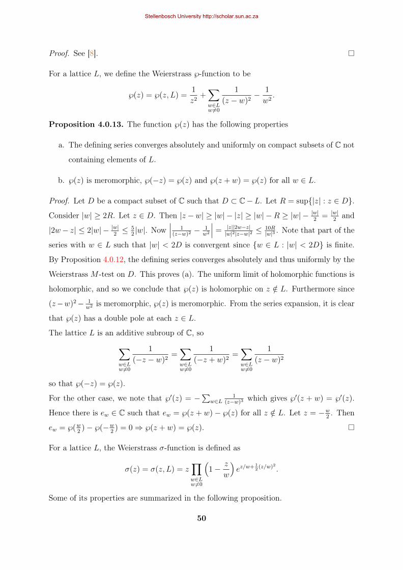
Proof. See [8].

For a lattice L, we define the Weierstrass ℘-function to be

℘(z) = ℘(z, L) =1

z2+∑w∈Lw 6=0

1

(z − w)2− 1

w2.

Proposition 4.0.13. The function ℘(z) has the following properties

a. The defining series converges absolutely and uniformly on compact subsets of C not

containing elements of L.

b. ℘(z) is meromorphic, ℘(−z) = ℘(z) and ℘(z + w) = ℘(z) for all w ∈ L.

Proof. Let D be a compact subset of C such that D ⊂ C−L. Let R = sup|z| : z ∈ D.

Consider |w| ≥ 2R. Let z ∈ D. Then |z −w| ≥ |w| − |z| ≥ |w| −R ≥ |w| − |w|2

= |w|2

and

|2w− z| ≤ 2|w| − |w|2≤ 5

2|w|. Now

∣∣∣ 1(z−w)2

− 1w2

∣∣∣ = |z||2w−z||w|2|z−w|2 ≤

10R|w|3 . Note that part of the

series with w ∈ L such that |w| < 2D is convergent since w ∈ L : |w| < 2D is finite.

By Proposition 4.0.12, the defining series converges absolutely and thus uniformly by the

Weierstrass M -test on D. This proves (a). The uniform limit of holomorphic functions is

holomorphic, and so we conclude that ℘(z) is holomorphic on z /∈ L. Furthermore since

(z−w)2− 1w2 is meromorphic, ℘(z) is meromorphic. From the series expansion, it is clear

that ℘(z) has a double pole at each z ∈ L.

The lattice L is an additive subroup of C, so∑w∈Lw 6=0

1

(−z − w)2=∑w∈Lw 6=0

1

(−z + w)2=∑w∈Lw 6=0

1

(z − w)2

so that ℘(−z) = ℘(z).

For the other case, we note that ℘′(z) = −∑

w∈L1

(z−w)3which gives ℘′(z + w) = ℘′(z).

Hence there is ew ∈ C such that ew = ℘(z + w)− ℘(z) for all z /∈ L. Let z = −w2. Then

ew = ℘(w2)− ℘(−w

2) = 0⇒ ℘(z + w) = ℘(z).

For a lattice L, the Weierstrass σ-function is defined as

σ(z) = σ(z, L) = z∏w∈Lw 6=0

(1− z

w

)ez/w+ 1

2(z/w)2 .

Some of its properties are summarized in the following proposition.

50


Proposition 4.0.14. The Weierstrass σ-function has the following properties

a. σ(z) is analytic.

b. σ(z) has simple zeros at w ∈ L and no other zeros.

c. d2

dz2log σ(z) = −℘(z).

d. For w ∈ L, there exist constants c = cw, d = dw such that

σ(z + w) = ecz+d for all z ∈ C.

Proof. a) Note that (1− y)ey+ 12y2 = 1 + b1y

3 + b2y4 + . . .. So for y near 0, we have

|(1− y)ey+ 12y2 − 1| = C|y|3

for some constant C. The inequality still holds when y = zw

for sufficiently large |w|

and z in a compact subset. Since∑| zw|3 converges by Lemma 4.0.12, it follows that∑(

(1− zw

)ezw

+ 12

( zw

)2 − 1)converges. From theory of infinite products, we know that if∑

n |bn| converges then∏

n(1+ bn) converges. Thus σ(z) converges uniformly on compact

subsets, and so σ(z) is analytic for all z ∈ C.

Part (b) is clear from the definition of σ(z).

c) We compute that

d

dzlog σ(z) =

1

z+∑w∈Lw 6=0

(1

z − w+

1

w+

z

w2

)

which implies that

d2

dz2log σ(z) = − 1

z2+∑w∈Lw 6=0

− 1

(z − w)2+

1

w2

= −℘(z).

d) Let w ∈ L. By chain rule ddz

log σ(z + w) = ddz

log σ(z), so that

d2

dz2log

σ(z + w)

σ(z)= 0.

Hence log σ(z+w)σ(z)

= cz + d and exponentiation yields the desired result. For possible

branches of the logarithm that may give rise to complications, refer to [10].

51


Theorem 4.0.15. Let D =∑ni[wi] with degD = 0 and

∑niwi ∈ L. Then there exists

an elliptic function g such that div(g) = D.

Proof. Let v =∑niwi and g(z) = σ(z)

σ(z−v)

∏i σ(z − wi)ni . Let w ∈ L. Then

g(z + w)

g(z)=σ(z − v + w)

σ(z − v)

−1σ(z + w)

σ(z)

∏i

(σ(z − wi + w)

σ(z − wi)

)ni.

But by Proposition 4.0.14 (d), there exist constants a, b depending on w such that

g(z + w)

g(z)= eaz+b · e−az+av−b

∏i

eni(a(z−wi)+b)

= 1 since∑i

ni = 0.

Therefore the function is elliptic. We also note that σ(z)σ(z−v)

is analytic at all z = wi which

means that the zeros or poles for g come from∏

i σ(z − wi)ni . Thus div(g) = D. Indeed

g is one such function that we desire.

4.1 Complex tori as elliptic curves

Definition 4.1.1. Associated to L and for an integer k ≥ 3, the Eisenstein series is given

by

Gk = Gk(L) =∑w∈Lw 6=0

w−k.

Clearly Gk = 0 for k odd as w ∈ L⇔ −w ∈ L.

Proposition 4.1.2. The functions ℘(z) and ℘′(z) satisfy the relation

℘′(z)2 = 4℘(z)3 − 60G4℘(z)− 140G6.

Proof. We will deduce the Laurent expansion of ℘(z) near 0. Recall that for |x| < 1,

1

1− x2=∑n≥0

(n+ 1)xn.

For |z| < |w|, we have

1

(z − w)2− 1

w2=

1

w2

(1

(1− zw

)2− 1

)=∑n≥1

(n+ 1)zn

wn+2.

52


which yields

℘(z) =1

z2+∑w∈Lw 6=0

∞∑n=1

(n+ 1)zn

wn+2

=1

z2+∞∑n=1

(n+ 1)zn∑w∈Lw 6=0

1

wn+2

=1

z2+∞∑i=1

(2i+ 1)z2i∑w∈Lw 6=0

1

w2j+2

=1

z2+∞∑i=1

(2i+ 1)G2i+2z2i

=1

z2+ 3G4z

2 + 5G6z4 + . . .

and so

℘′(z) = − 2

z3+ 6G4z + 20G6z

3 + . . .

By expansion, we obtain

℘(z)3 =1

z6+

9

z2G4 + 15G6 + . . .

℘′(z) =4

z6− 24

z2G4 − 80G6 + . . .

and note that g(z) defined by

g(z) = ℘′(z)2 − 4℘(z)3 + 60G4℘(z) + 140G6

has no constant term and no negative powers of z and clearly g(z) ∈ C(℘(z), ℘(z)). So

g(z) is doubly periodic and is holomorphic at 0. Hence it has no poles. Thus g(z) is

constant. Using its series expansion, we note that g(z) = 0. This yields the desired

result.

We shall let g3 = 140G6 and g2 = 60G4. Note that the discriminant of the polynomial

4x3 − g2x− g3 is 16(g32 − 27g2

3).

Proposition 4.1.3. g32 − 27g2

3 6= 0

53


Proof. As ℘′(z) is elliptic, we have ℘′(z + wi) = ℘′(z) for all z ∈ C and i = 1, 2, 3. Set

z = −wi2. Then ℘′(−wi

2) = ℘′(wi

2). From the relation ℘′(−z) = −℘′(z), it follows that

℘′(wi2

) = 0. Hence ℘(wi2

) is a root of the polynomial 4x3 − g2x − g3. We now show that

the roots of the polynomial are distinct.

Let fi(z) = ℘(z) − ℘(wi2

). Then fi(wi2 ) = 0 and f ′i(wi2

) = 0. Thus fi(z) has a vanishing

order of at least 2 at wi2. But fi(z) has only one pole in Π at z = 0, and it is a double

pole. By Theorem 4.0.10 (c), wi2

is the only root of fi(z). So fi(wj2

) 6= 0 for i 6= j which

implies that 4x3 − g2x− g3 has distinct roots.

Consequently E : y2 = 4x3− g2x− g3 is an elliptic curve. We have the following theorem.

Theorem 4.1.4. Let E/C be the elliptic curve defined by y2 = 4x3 − g2x− g3 and L be

a lattice. Then the map Φ : C/L→ E(C) given by

z 7→ (℘(z), ℘′(z))

0 7→ O

is a group isomorphism.

Proof. We divide the proof into two parts. The first shows bijectivity and the second

shows that Φ is a homomorphism.

Let (x, y) ∈ E(C). Consider the function ℘(z)− x. This function has a double pole, and

so it has zeros. Hence, there is z ∈ C such that

℘(z) = x and ℘′(z)2 = y2.

Thus ℘′(z) = ±y. If ℘(z) = y, then we are done. Now suppose that ℘′(z) = −y. Then

℘′(−z) = y. We also have ℘(−z) = ℘(z) = x so that −z 7→ (x, y). Surjectivity is proved.

Suppose (℘(z1), ℘′(z1)) = (℘(z2), ℘′(z2)). If z1 is a pole of ℘(z), then z1, z2 ∈ L since ℘(z)

only has poles in L and no where else. Then z1 ≡ z2 mod L. On the other hand, if z1 is

not a pole of ℘(z), then z1 /∈ L. Since ℘(z) has a double pole at z = 0 and no other poles

in Π, it follows that r(z) = ℘(z)−℘(z1) has a double pole at z = 0 and no other poles in

Π. By Theorem 4.0.10 (c), r(z) has two zeros.

Suppose z1 = wi2

for some i ∈ 1, 2, 3. Since ℘′(wi2

) = 0, z1 is a double zero of r(z), and

thus the only zero. By our earlier assumption, we know that z2 is a root of r(z). Hence

54


z1 = z2 ⇒ z1 ≡ z2 mod L.

Now suppose that z1 6= wi2

for some i ∈ 1, 2, 3. Then 2z1 /∈ L ⇒ z1 + z1 6≡ 0 mod L.

But r(z1) = r(−z1) = 0 implies that the two zeros of r(z) are z1 mod L and −z1 mod L.

So we must have z2 ≡ −z1 mod L. We also have

y = ℘′(z2) = ℘′(−z1) = −℘′(z1) = −y

which implies ℘′(z1) = 0. We know that ℘′(z) has only triple pole in Π, and thus it

has three zeros. We also know that wi2

are the three zeros of ℘′(z). This contradicts

our assumption that z1 6= wi2

for some i ∈ 1, 2, 3. Thus z1 ≡ z2 mod L, establishing

injectivity.

We now prove the homomorphism property of Φ. Let P1 = (x1, y1), P2 = (x2, y2) be

distinct points such that the straight line passing through them intersects E at point

P3 = (x3, y3) such that P3 6= P1 and P3 6= P2. We set Pi = Φ(zi).

Let y = λx + µ be the straight line through P1 and P2. By computing the addition

formula, we note that

x3 =1

4

(y2 − y1

x2 − x1

)2

− x1 − x2

=1

4

(℘′(z2)− ℘′(z1)

℘(z2)− ℘(z1)

)2

− ℘(z1)− ℘(z2).

From the line, we see that ℘′(zi) = λ℘(zi)+µ so that the function t(z) = ℘′(z)−λ℘(z)−µ

has zeros at z1, z2 and z3. However t(z) is elliptic and has a triple pole at z = 0 and no

poles in Π. Hence t(z) has three zeroes in C. Thus div(t) = [z1] + [z1] + [z1]− 3[O] which

implies that∑

w∈L ordw(t) · w ∈ L by Theorem 4.0.10 (b). We have z1 + z2 + z3 ∈ L ⇒

z1 + z2 = −z3 mod L⇒ ℘(z1 + z3) = ℘(−z3) = ℘(z3) = x3. So we have

℘(z1 + z2) =1

4

(℘′(z2)− ℘′(z1)

℘(z2)− ℘(z1)

)2

− ℘(z1)− ℘(z2). (4.1.1)

Fixing z1 and differentiating the left hand side of Equation 4.1.1, we obtain an expression

of ℘′(z1 + z2) in terms of xi = ℘(zi), yi = ℘′(zi) for i = 1, 2 and ℘′′(z2). From the

Weierstrass equation, we note that

2℘′′(z) = 12℘(z)2 − g2 for ℘′(z) 6= 0. (4.1.2)

55


For the case ℘′(z) = 0, refer to [10]. Setting z = z2 and substituting in the the expression

for ℘′′(z1 + z2) and performing some algebraic manipulation, we get −y3 = ℘′(z1 + z2).

Thus

Φ(z1 + z2) = Φ(z1) + Φ(z2). (4.1.3)

We now look at the cases where ℘(z1 + z2) in Equation 4.1.1 is not defined, i.e ℘(zi) =∞

or z1 = −z2.

When ℘(zi) =∞, then zi is a pole and poles of ℘(z) only occur at points in L. So zi = 0.

Hence (℘(0), ℘(0)) = O which shows that Equation 4.1.3 is true. For z1 = −z2, we have

z1 + z2 = 0 mod L so that Φ(z1 + z2) = O. We also note that

(℘(z2), ℘′(z2)) = (℘(z1), ℘′(−z1)) = (℘(z1),−℘′(z1)) = −(℘(z1), ℘′(z1))

which implies (℘(z1), ℘′(z1)) + (℘(z2), ℘′(z2)) = O. Thus Equation 4.1.1 is true. For the

case when z1 = z2, we note that ℘′(z2)−℘′(z1)℘(z2)−℘(z1)

→ ℘′′(z2)℘′(z2)

as z1 → z2 by L’Hopital’s rule and

using Equations 4.1.1 and 4.1.2, we have

℘(2z1) =1

4

(6℘(z1)2 − 1

2g2

℘′(z1)

)2

− 2℘(z1).

Using appropriate group law formulas, it can be shown that if x1 = x3, then

x3 =1

4

(12x1 − g2

2y1

)2

− 2x1.

Clearly x3 = ℘(2z1). Differentiating with respect to z1 yields the right expression for the

y-coordinate.

4.2 Uniformization theorem

We now want to show that every elliptic curve comes from a lattice.

Consider L = Zw1 +Zw2. The R-linear independence of w1 and w2 implies that τ = w1

w2∈

C \ R. By rearrangement if necessary, we may assume that Im(τ) > 0. Thus we have

another lattice Lτ = Zτ +Z. Since w2Lτ = L, the two lattices Lτ and L are homothetic.

For an integer k ≥ 3, define

Gk(τ) = Gk(Lτ ) =∑

(r,s)6=(0,0)

1

(rτ + s)k.

56


Then we have Gk(τ) = wk2Gk(L) where Gk(L) is the Eisenstein series for the lattice

L = Zw1 + Zw2.

Let g2(τ) = g2(Lτ ) = 60G4(τ) and g3(τ) = g3(Lτ ) = 140G6(τ). Let ∆ = g32 − 27g2

3 and

define

j(τ) = 1728g3

2

∆. (4.2.1)

In general, for an arbitrary lattice L, we define j(L) to be

j(L) = 1728g2(L)3

g2(L)3 − 27g3(L)2.

It can be shown that j(L) converges and we will not concern ourselves of the details of

the proof, and for such details we refer you to [10]. So it follows that for any λ ∈ C×,

g2(λL) = λ−4g2(L) and g3(λL) = λ−6g3(L).

Hence j(λL) = j(L). In particular j(Zw1 + Zw2) = j(τ) where τ = w1

w2.

Let H denote the upper half plane. Also note the action of SL2(Z) on H given bya b

c d

τ =aτ + b

cτ + d

for all τ ∈ H.

Proposition 4.2.1. For any τ ∈ H and

a b

c d

∈ SL2(Z), we have

j(τ) = j

(aτ + b

cτ + d

)Proof. By definition, we have

Gk

(aτ + b

cτ + b

)=

∑(r,s)6=(0,0)

1(r aτ+bcτ+d

+ s)k

= (cτ + d)k∑

(r,s)6=(0,0)

1

((ra+ sc)τ + rb+ sd)k

Let (r′, s′) = (ra + sc, rb + sd) = (r, s)

a b

c d

. Then (r, s) = (r′, s′)

a b

c d

−1

. Thus

we have a 1-1 correspondence between pairs of integers (r, s) and (r′, s′). Hence

Gk

(aτ + b

cτ + b

)= (cτ + d)k

∑(r′,s′)6=(0,0)

1

(r′τ + s′)k

= (cτ + d)kGk(τ).

57


So we note that

g2

(aτ + b

cτ + b

)= 60G4

(aτ + b

cτ + b

)= (cτ + d)460G4(τ)

= (cτ + d)4g2(τ).

Similarly, we have g3

(aτ+bcτ+b

)= (cτ + d)6g3(τ). Substituting these expressions in Equation

4.2.1 yields the result.

Let Hf = z ∈ H : −12≤ Re(z) < 1

2, z 6= eiθ for π

3< θ < π

2, |z| ≥ 1. Hf is called the

fundamental domain of H under the action of SL2(Z).

Proposition 4.2.2. For every τ ∈ H, there is M ∈ SL2(Z) such that Mτ ∈ Hf and Mτ

is uniquely determined by τ .

Proof. See [10].

Corollary 4.2.3. For any lattice L, there exists a basis w1, w2 such that w1

w2∈ Hf .

Proof. Let y1, y2 be a basis of L. Performing a rearrangement if necessary, we may

assume that t = y1y2∈ H. By Proposition 4.2.2, let

a b

c d

∈ SL2(Z) be such that

at+bct+d∈ Hf . Set w1 = ay1 + by2 and w2 = cy1 + dy2. Clearly, Zy1 +Zy2 = Zw1 +Zw2 sincea b

c d

is invertible. Furthermore,

w1

w2

=ay1 + by2

cy1 + dy2

=a(y1/y2) + b

c(y1/y2) + d=at+ b

ct+ d∈ Hf .

Proposition 4.2.4. For every complex number z, there is exactly one τ ∈ Hf such that

j(τ) = z.

Proof. See [8].

Corollary 4.2.5. Let τ1 and τ2 be elements in H. Then j(τ1) = j(τ2) if and only if there

exists M ∈ SL2(Z) such that Mτ1 = τ2.

58


Proof. If there exists M ∈ SL2(Z) such that Mτ1 = τ2, then Proposition 4.2.1 tells us

that j(τ) = j(Mτ) = j(τ).

Conversely, suppose that j(τ1) = j(τ2). By Proposition 4.2.2, there exist M ′,M ′′ ∈

SL2(Z) such that

M ′τ1 = τ ′1 ∈ Hf and M ′′τ2 = τ ′2 ∈ Hf .

So we observe that j(τ1) = j(M ′τ1) = j(τ ′1) and j(τ2) = j(M ′′τ2) = j(τ ′1) which implies

that j(τ ′1) = j(τ ′2). By Proposition 4.2.4, it follows that τ ′1 = τ ′2.

It is not difficult to see that M ′′τ2 = τ ′2 for M ′′ ∈ SL2(Z) implies that N ′′τ ′2 = τ2 for some

N ′′ ∈ SL2(Z). Thus we can find M ∈ SL2(Z) such that Mτ1 = τ2.

Corollary 4.2.6. Let L′, L′′ be arbitrary lattices in C. Then j(L′) = j(L′′) if and only

if L′ = cL′ for some constant c ∈ C×.

Proof. If L′ = cL′, c ∈ C×, then we saw earlier that j(cL′) = j(L′) so that this direction

is verified.

Conversely, if j(L′) = j(L′). By Corollary 4.2.3, L′ = r1Lτ1 and L′′ = r2Lτ2 for some

τi ∈ Hf and ri ∈ C×, i = 1, 2. So we have

j(Lτ1) = j(τ1) = j(Lτ2) = j(τ2)

and by Proposition 4.2.4, we have τ1 = τ2. Setting c = r1r2, we have L′ = cL′′.

Theorem 4.2.7. Let E/C be an elliptic curve defined by the equation y2 = 4x3−Ax−B.

Then there exists a lattice L such that g2(L) = A and g3(L) = B. Furthermore, we have

a group isomorphism C/L ∼= E(C).

Proof. Let z = 1728 A3

A3−27B2 . Proposition 4.2.4 implies that there is a lattice T = Zτ +Z

where τ ∈ Hf such that j(T ) = j(τ) = z, i.e

1728g2(T )3

g2(T )3 − 27g3(T )2= 1728

A3

A3 − 27B2. (4.2.2)

We investigate the following situations.

Case I: Suppose g2(T ) 6= 0. Then A 6= 0 since g2(T )3 − 27g3(T )2 6= 0 by Proposition

4.1.3 and A3 − 27B2 6= 0 as E is an elliptic curve. Choose c ∈ C× with the property

that g2(cT ) = c−4g2(T ) = A. Then by some algebraic manipulation of Equation 4.2.2,

59


we have g3(cT )2 = B2 ⇒ g3(cT ) = ±B. If g3(cT ) = B, then L = cT is a desired lattice.

Otherwise, we observe that

g3(icT ) = i−6g3(cT ) = −g3(cT ) = B and g2(icT ) = i−4g2(cT ) = A

so that L = icT is a desired lattice.

Case II: Assume g2(T ) = 0. Then A = 0, B 6= 0 and g3(T ) 6= 0. So choose d ∈ C× such

that g3(dT ) = d−6g3(T ) = B. Then g2(dT ) = d−4g2(T ) = 0. Thus L = dT is a desired

lattice.

By Theorem 4.1.4, C/L ∼= E(C).

The structure of E[m] is now easy to describe. Since there exists a lattice L = Zw1 +Zw2

such that E(C) ∼= C/L and that we can identify C/L with the fundamental parallelogram,

we have that z ∈ E[m] if and only if z = jmw1 + k

mw2 where 0 ≤ j, k < m and j, k ∈ Z.

Thus

E[m] ∼= Z/mZ× Z/mZ

which also confirms the result in chapter three on the structure of m-torsion subgroup

when char K = 0. We demonstrate this with an example for m = 2, 3.

Example 4.2.8 (The case of m = 2). Let E/C be given by the equation y2 = f(x) where

f(x) = x3 + ax2 + bx+ c.

For m = 2, recall that P has order two if and only if 2P = O and P 6= O. But 2P = O

implies P = −P so that x(P ) = x(−P ). This means that the y-coordinate of P must be

zero. Conversely, if P = (x, 0), then the tangent at P is vertical so that 2P = O. Hence

points of order two are exactly those points whose y coordinate is equal to zero. We have

to solve the equation f(x) = 0, for the x coordinates. By the fundamental theorem of

algebra, f has three complex roots. We have three points P 6= O with order dividing 2.

Together with O, the three points of order two form an abelian subgroup of E(C). Thus

E[2] ∼= Z/2Z× Z/2Z

since there are no points of order 4.

60


Example 4.2.9 (The case of m = 3). We now look at the case when m = 3 using the

curve defined in Example 4.2.8. If P has order three, then 3P = O which is the same

as saying 2P = −P . So we have x(2P ) = x(P ). We claim that if x(2P ) = x(P ) and

P 6= O, then 3P = O. That is because x(2P ) = x(P ) implies that x(2P ) = x(−P ) so

that 2P = ±P which implies 3P = O since P 6= O. Hence points of order three in E(C)

are exactly those points that satisfy the equality x(2P ) = x(P ). Let P = (x, y). Using

appropriate group law formulas, we have

x4 − 2bx2 − 4ac+ b2 − 8cx− 4x(ax2 + x3 + bx+ c) = 0

which results in

3x4 + 4ax3 + 6bx2 + 12cx+ 4ac− b2 = 0.

So points of order three are the roots of the equation 3x4+4ax3+6bx2+12cx+4ac−b2 = 0

Furthermore, we also observe that

3x4 + 4ax3 + 6bx2 + 12cx+ 4ac− b2 = 2f(x)f ′′(x)− f ′(x)2.

Denote this polynomial by β(x). Then β′(x) = 12f(x). We claim that each complex zero

of β(x) has multiplicity 1. To justify this claim, it is enough to show that β(x) and β′(x)

have no common zero.

Assume that β(x) and β′(x) have a common zero α, say. It follows that α is a root of

12f(x) and 2f(x)f ′′(x) − f ′(x)2, i.e f(α) = 0 and 2f(α)f ′′(α) − f ′(α)2 = 0. Clearly we

have f(α) = 0 and f ′(α) = 0 so that α is a common zero of f(x) and f ′(x). This implies

that E is singular. So we have a contradiction. Hence β(x) and β′(x) have no common

root implying that the polynomial β(x) has distinct roots. Since its degree is 4, we have

four distinct roots. However note that each root gives two values of y so that we have

exactly eight points of order three. Consequently, there are nine points of order dividing

three (we have included the identity). Hence E[3] ∼= Z/3Z× Z/3Z.

61


Chapter 5

Elliptic curves over local fields


5.1 Formal Groups

Definition 5.1.1. A (one-parameter commutative) formal group F over a ring R is a

power series F (X, Y ) ∈ R[[X, Y ]] satisfying the following properties:

1. F (X, Y ) = X + Y + (terms of higher degree ≥ 2).

2. F (X, Y ) = F (Y,X) (Commutativity).

3. F (X,F (Y, Z)) = F (F (X, Y ), Z) (Associativity).

4. F (X, 0) = X and F (0, Y ) = Y .

5. There exits a unique i(T ) ∈ R[[T ]] such that F (i(T ), T ) = 0 (existence of inverse).

The power series F (X, Y ) is called the formal group law of F .

It is easy to see that F (X, Y ) = X + Y defines is a formal group with i(T ) = −T .

Definition 5.1.2. Let (F,F) and (G,G) be formal groups over a ring R. A homomor-

phism from F to G (defined over R) is a power series f ∈ R[[T ]] such that f(F (X, Y )) =

G(f(X), f(Y )). In addition to the above, if there exists a homomorphism g : G → F

with g(f(T )) = f(g(T )) = T , then F and G are said to be isomorphic over R

62


Proposition 5.1.3. Let (F,F) be a formal group and m ∈ Z. Then [m] : F → F defined

by

[0](T ) = 0, [m+ 1](T ) = F ([m](T ), T ), [m− 1](T ) = F ([m](T ), i(T ))

is a homomorphism

Proof. We look at the case m ≥ 0. Clearly [0](F (X, Y )) = F ([0](X), [0](Y )). By induc-

tion assume the result holds for an integer k ≥ 1, i.e [k](F (X, Y )) = F ([k](X), [k](Y )).

We need to show that it is true for k + 1. We proceed as follows:

[k + 1](F (X, Y )) = F ([k](F (X, Y ), F (X, Y )) by definition

= F (F ([k](X), [k](Y )), F (X, Y )) by induction hypothesis

= F ([k](X), F ([k](Y ), F (X, Y ))) by associativity

= F ([k](X), F (F (X, Y ), [k](Y ))) by commutativity

= F ([k](X), F (X,F (Y, [k](Y )))) by associativity

= F ([k](X), F (X,F ([k](Y ), Y ))) by commutativity

= F (F ([k](X), X), F ([k](Y ), Y )) by associativity

= F ([k + 1](X), [k + 1](Y ))

Before proving for m ≤ −1, we claim that iF (X, Y ) = F (i(X), i(Y )). By definition, we

have

F (F (X, Y ), i(F (X, Y ))) = 0 (5.1.1)

and so using associativity and commutativity, we observe that

F (F (X, Y ), F (i(X), i(Y ))) = F (X,F (F (i(X), i(Y )), Y ))

= F (F (X,F (i(X), i(Y ))), Y ).

But the inner term F (X,F (i(X), i(Y ))) = F (F (X, i(X)), i(Y )) = F (0, i(Y )) = i(Y )

so that F (F (X,F (i(X), i(Y ))), Y ) = F (i(Y ), Y ) = 0. By uniqueness of i(F (X, Y ) in

Equation 5.1.1, we conclude that F (i(X), i(Y )) = iF (X, Y ). Let m = −1. Then

[−1](F (X, Y )) = F ([0](F (X, Y ), i(F (X, Y )))) = iF (X, Y ) which by the above claim

63


is F (i(X), i(Y )). But

F (i(X), i(Y )) = F (0, F (i(X), i(Y ))) = F (0, F (i(X), F (0, i(Y ))))

= F (F (0, i(X)), F (0, i(Y ))) = F ([−1](X), [−1](Y )).

Assume it holds for an integer k < 0, i.e [k](F (X, Y ) = F ([k](X), [k](Y )). We note that

[k − 1](F (X, Y )) = F ([k](F (X, Y )), i(F (X, Y )))

= F (F ([k](X), [k](Y )), F (i(X), i(Y )))

= F (F ([k](Y ), [k](X)), F (i(X), i(Y )))

= F ([k](Y ), F ([k](X), F (i(X), i(Y )))). But we have

F ([k](X), F (i(X), i(Y ))) = F (F ([k](X), i(X)), i(Y )) = F ([k − 1](X), i(Y ))

so that [k − 1](F (X, Y )) = F ([k](Y ), F ([k − 1](X), i(Y )))

= F ([k](Y ), F (i(Y ), [k − 1](X)))

= F (F ([k](Y ), i(Y )), [k − 1](X))

= F ([k − 1](Y ), [k − 1](X)).

Proposition 5.1.4. If f(T ) = a1T + a2T2 + a3T

3 + a4T4 + . . . ∈ R[[T ]] with a1 ∈ R×,

then there exists a unique power series g(T ) satisfying f(g(T )) = g(f(T )) = T .

Proof. Note that constructing a sequence gn(T ) such that f(gn(T )) ≡ T (mod T n+1) and

gn+1(T ) ≡ gn(T ) (mod T n+1), and setting

g(T ) = limn→∞

gn(T )

proves the existence part. Set g1(T ) = a−11 T and clearly f(g1(T )) ≡ T (mod T 2). Having

defined gn−1, we by induction define

gn(T ) = gn−1(T ) + λT n

64


for some λ ∈ R to be determined. So we have

f(gn(T )) = f(gn−1(T ) + λT n)

= a1(gn−1(T ) + λT n) + a2(gn−1(T ) + λT n)2 + a3(gn−1(T ) + λT n)3 + . . .

≡ a1λTn + a1gn−1(T ) + a2gn−1(T )2 + a3gn−1(T )3 + . . . (mod T n+1)

≡ f(gn−1(T )) + a1λTn (mod T n+1)

≡ T + cT n + a1λTn (mod T n+1) for some c ∈ R.

From the relation f(gn(T )) ≡ T (mod T n+1), we obtain λ = −a−11 c. By this construction,

we have that g(T ) ∈ R[[T ]] and satisfies f(g(T )) = T . On the other hand, we have

g(T ) = a−11 T+(terms of higher order) and a−1

1 ∈ R×. By the above argument, there exists

g′(T ) ∈ R[[T ]] such that g(g′(T )) = T . So g(f(T )) = g(f(g(g′(T )))) = g(f g(g′(T ))) =

g(g′(T )) = T . Finally to prove uniqueness of g(T ). Assume that h(T ) is another power

series satisfying f(h(T )) = T . Then g(T ) = g(f h(T )) = (g f)(h(T )) = h(T ).

Proposition 5.1.5. Let F be a formal group over R and m ∈ Z. Then

a. [m](T ) = mT + higher order terms.

b. If m ∈ R×, then [m] : F → F is an isomorphism.

Proof. For m ≥ 0, using the recursive definition of [m](T ) given in Proposition 5.1.3

and induction on m yields (a). Now suppose that m < 0. By definition, [−1](T ) =

F ([0](T ), i(T )) = F (0, i(T )) = i(T ). But F (T, i(T )) = 0⇒ 0 = T + i(T ) + . . .⇒ i(T ) =

−T + . . .. Applying a downward induction on m completes the general case m < 0.

(b) Follows from Proposition 5.1.4.

Definition 5.1.6. Let R be a complete local ring with maximal idealM and F a formal

group over R. The group associated to F/R, denoted by F(M), is the setM endowed

with the operations

x⊕ y = F (x, y) for all x, y ∈M (addition).

x = i(x) for all x ∈M (inversion).

Note that F(M) is a group under the stated operations.

65


Proposition 5.1.7. Let F be a formal group over a complete local ring R with the

maximal idealM and p = charR/M > 0. Then F(M) is a p-group.

Proof. Let x ∈ F(M) be an element of order m. Then [m](x) = 0. Write m = rps with

(p, r) = 1. Then we have [r]([ps](x)) = 0. So we can assume that (m, p) = 1. Then

[m](x) = 0 and m ∈ R×. By Proposition 5.1.5, [m] : F(M)→ F(M) is an isomorphism,

and thus x = 0.

We would like to look at the formal group associated to an elliptic curve. We first discuss

the following.

Proposition 5.1.8. (Hensel’s Lemma) Let R be a ring that is complete with respect to

some ideal I ⊂ R. Suppose F (T ) ∈ R[T ], a ∈ R, n ∈ Z≥1 are such that F (a) ∈ In and

F ′(a) ∈ R×. If α ≡ F ′(a) (mod I), then

w0 = a, wm+1 = wm −F (wm)

α

converges to b ∈ R such that b is a zero of F (T ) and b ≡ a (mod In). If R is an integral

domain, then b is unique.

Proof. We replace F (w) by F (w+a)α

so that the above conditions and recurrence become:

F (0) ∈ In, F ′(0) ≡ 1 (mod I) , w0 = 0, wm+1 = wm − F (wm).

We first prove the convergence part. Note that w1 = w0 − F (0) ∈ In ⇒ w2 ∈ In.

Continuing in this manner, we see that if wm ∈ In, then wm+1 ∈ In for all m ≥ 0. By

induction, it follows that wm ∈ In for all m ≥ 0.

We claim that wm+1 − wm ∈ Im+n for all m ≥ 0. Clearly w1 − w0 = −F (0) ∈ In.

By induction, assume it is true for all integers strictly less than m. Note that F (T ) =

F (0) + F ′(0)T +O(T 2), and so we can write

F (s)− F (t) = (s− t)(F ′(0) + sG(s, t) + tH(s, t)) for some G,H ∈ R[s, t]. (5.1.2)

By the recurrence relation, we have

wm+1 − wm = wm − F (wm)− (wm−1 − F (wm−1)) = wm − wm−1 − (F (wm)− F (wm−1))

66


and so using Equation 5.1.2,

F (wm)− F (wm−1) = (wm − wm−1)(F ′(0) + wmG(wm, wm−1) + wm−1H(wm, wm−1))

so that

wm+1 − wm = (wm − wm−1)(1− F ′(0)− wmG(wm, wm−1)− wm−1H(wm, wm−1)).

Since 1− F ′(0) ∈ I, wm−1, wm ∈ In ⊆ I, it follows that

(1− F ′(0)− wmG(wm, wm−1)− wm−1H(wm, wm−1)) ∈ I

and by induction hypothesis, wm − wm−1 ∈ Im−1+n, we have wm+1 − wm ∈ Im−1+nI =

Im+n. The completeness of R implies convergence of the sequence to an element b ∈ In

such that b = b− F (b), i.e F (b) = 0.

For the uniqueness part where we assume that R is an integral domain, say c ∈ In

is such that F (c) = 0. Making use of Equation 5.1.2, observe that F (b) − F (c) =

(b − c)(F ′(0) + bG(b, c) + cH(b, c)) = 0. If b 6= c, then F ′(0) = −bG(b, c) − cH(b, c) ∈ I

as b, c ∈ I. But this is a contradiction since F ′(0) /∈ I. So we must have b = c.

Definition 5.1.9. Let F be a formal group over a ring R with the formal group law

F . An invariant differential on F is a differential form ω(T ) = P (T )dT that satisfies

ω(F (T, S)) = ω(T ).

From the definition above, we have

ω(F (T, S)) = ω(T )⇒ P (F (T, S))d(F (T, S)) = P (T )dT

which implies that P (F (T, S)) ∂∂T

(F (T, S)) = P (T ). We use F1(U, V ) to mean the partial

derivative of F with respect to the first variable. So w(T ) = P (T )dT is invariant if

P (F (T, S))F1(T, S) = P (T ). If P (0) = 1, ω is said to be normalized.

Proposition 5.1.10. For a formal group F/R with formal group law F , there exists a

unique invariant differential given by F1(0, T )−1dT such that if ω is an invariant differen-

tial on F , then ω = λF1(0, T )dT for some λ ∈ R.

67


Proof. Let ω be an invariant differential. Now ω = P (T )dT is such that

P (F (T, S))F1(T, S) = P (T )⇒ P (F (0, S))F1(0, S) = P (0),

i.e P (S)F1(0, S) = P (0). But

F (T, S) = S + T + higher order terms ⇒ F1(0, S) = 1 + higher order terms

so that F1(0, T )−1 ∈ R[[T ]]. Thus P (T ) = P (0)F1(0, T )−1. Since we know the coefficients

of F1(0, T )−1, we just need to know P (0) to completely specify P (T ). So if P (0) = 1,

we have P (T ) = F1(0, T )−1 and the differential F1(0, T )−1dT is unique and normalized

differential. As shown above, ω is of the form λF1(0, T )−1. It remains to show that

F1(0, T )−1dT is invariant, i.e

F1(0, F (T, S))−1F1(T, S) = F1(0, T )−1.

Recall the associativity law F (X,F (T, S)) = F (F (X,T ), S). Differentiating with respect

to X we have

F1(X,F (T, S)) =∂

∂R(F (R, S))F1(X,T ) where R = F (X,T ),

which, in our notation implies that

F1(X,F (T, S)) = F1(F (F (X,T ), S))F1(X,T ).

Set X = 0, we get

F1(0, F (T, S)) = F1(F (T, S))F1(0, T )

which yields the desired result.

Proposition 5.1.11. Let f : F/R→ G/R be a homomorphism between formal groups.

Let ωG and ωF be normalised invariant differentials on F/R and G/R, respectively. Then

ωG f = f ′(0)ωF .

Proof. Denote by F,G ∈ R[[X, Y ]] the formal group laws of F and G, respectively. Then

(ωG f)(F (T, S)) = ωG(G(f(T ), f(S))) = ωG(f(T )) = (ωG f)(T )

68


Thus ωG f is an invariant differential on F . So by Proposition 5.1.10, ωG f = λωF for

some λ ∈ R. To find λ, note that

ωG(f(T )) = G1(0, f(T ))−1df(T ) = G1(0, f(T ))−1f ′(T )dT

and

λωF = λF1(0, T )−1dT

so that

f ′(T ) = λF1(0, T )−1G1(0, f(T )) = λ(1 + higher order terms)

from which we get λ = f ′(0).

Proposition 5.1.12. Given a formal group F/R and a prime p ∈ Z. There exist

g(T ), h(T ) ∈ R[[T ]] such that h(0) = g(0) = 0 and [p](T ) = ph(T ) + g(T p).

Proof. Recall that [p](T ) = pT + higher order terms ⇒ [p]′(0) = p. Let ω be the

normalized differential on F . Then Proposition 5.1.11 says that

pω(T ) = (ω [p])(T ) = F1(0, [p](T ))−1d([p](T )) = (1 + higher order terms)[p]′(T )dT

which implies that

[p]′(T ) ∈ pR[[T ]] since (1 + higher order terms)−1 ∈ R[[T ]].

Hence a term biTi is such that p|i or p|bi.

Theorem 5.1.13. Let R be a discrete valuation ring which is complete with respect to its

maximal idealM and v be the valuation on R. Assume char R = 0 and p = charR/M >

0 and let F/R be a formal group. Let z be a non-zero torsion element of F(M) of order

pn for some positive integer n. Then

v(z) ≤ v(p)

pn − pn−1.

Proof. Let H be the cyclic subgroup of F(M) generated by z. Consider its subgroup

H[pn−1] = x ∈ H : [pn−1](x) = 0

and let H−H[pn−1] = z1, z2, . . . , zh. Clearly zi = niz for some ni satisfying 1 ≤ ni < pn

and (p, ni) = 1. Hence h = |i : (i, pn) = 1| = pn − pn−1. Since (p, ni) = 1, we must

69


have ni ∈ R× so that v(zi) = v(z) for all i. Write [p](T ) = Tu(T ) where u(0) = p. Define

w(T ) = u([pn−1](T )). Then w(0) = p and [pn](T ) = [p]([pn−1](T )) = [pn−1](T )w(T ). We

then have [pn−1](zi) 6= 0 and [pn](zi) = [pn−1](zi)w(zi) = 0 so that

w(zi) = 0⇒ w(T ) = (T − z1)(T − z2)(T − z3) . . . (T − zh)f(T ) where f(T ) ∈ R[[T ]].

Setting T = 0, we find that v(p) ≥ v(z1) + v(z2) + . . .+ v(zh) = hv(z) = (pn − pn−1)v(z)

which proves the result.

Now we examine the local group structure of an elliptic curve near the identity.

Consider the Weierstrass equation E : y2 + a1xy + a3y = x3 + a2x2 + a4x+ a6. Consider

the change of variables z = −xyand w = − 1

y. The fact that z is a uniformizer at O

has already been proven. In projective coordinates the transformation is (X : Y : Z) 7→

(−X : −Z : Y ) so that O 7→ (0, 0) on the following affine piece whose equation is obtained

by the change of variables above

w = z3 + (a1z + a2z2)w + (a3 + a4z)w2 + a6w

3. (5.1.3)

Let f(z, w) = z3 + (a1z + a2z2)w + (a3 + a4z)w2 + a6w

3. We can write w as a formal

power series in terms of z by repeated substitution of w = f(z, w) as follows

w = f(z, w)

= z3 + (a1z + a2z2)w + (a3 + a4z)w2 + a6w

3

= z3 + (a1z + a2z2)(z3 + (a1z + a2z

2)w + (a3 + a4z)w2 + a6w3)

+ (a3 + a4z)(z3 + (a1z + a2z2)w + (a3 + a4z)w2 + a6w

3)2

+ a6(z3 + (a1z + a2z2)w + (a3 + a4z)w2 + a6w

3)3 + . . .

Proposition 5.1.14. Indeed the above process converges and gives a formal power series

w(z) ∈ Z[a1, a2, a3, a4, a6][[z]] satisfying w(z) = f(z, w(z)).

Proof. Let R = Z[a1, a2, a3, a4, a6][[z]], α = −1, I = 〈z〉, a = 0 and F (w) = f(z, w)− w.

Since F ′(0) = −1 + a1z + a2z2 ∈ R×, F (0) = 0 and F ′(0) ≡ −1 (mod I), we conclude by

the version of Hensel’s Lemma in Proposition 5.1.8, that there exists a unique w(z) such

that f(z, w(z)) = w(z).

70


Making further substitutions, we realize that

w(z) = z3 + a1z4 + (a2

1 + a2)z5 + (a1z3 + 2a1a2 + a3)z6 + . . . ,

and thus in general, we have

w(z) = z3(1 +A1z+A2z2 +A3z

3 + . . .) for some A1, A2, . . . ∈ Z[a1, a2, a3, a4, a6]. (5.1.4)

Proposition 5.1.15. There exist power series i(z), F (z1, z2) ∈ Z[a1, a2, a3, a4, a6][[z]] such

that [−1](z, w(z)) = (i(z), w(i(z))) and

(z1, w(z1)) + (z2, w(z2)) = (F (z1, z2), w(F (z1, z2)))

where + is the addition on the new curve described by Equation 5.1.3.

Proof. Let z1 and z2 be independent indeterminates and set P1 = (z1, w1), P2 = (z2, w2)

with w1 = w(z1), w2 = w(z2). The points lie on the curve given by Equation 5.1.3. Then

using (0, 0) as the origin, we can determine the sum P3 = P1 + P2. The line through the

points has slope

λ = λ(z1, z2) =w(z2)− w(z2)

z2 − z1

=∞∑k=3

Ak−3zk2 − zk1z2 − z1

which is in Z[a1, a2, a3, a4, a6][[z]]. So the straight line has equation w = λz + µ where

µ = w1−λz1, and substituting in Equation 5.1.3 and making rearrangements, we observe

that z3 ∈ Z[a1, a2, a3, a4, a6][[z]]. Let w3 = λz3 + µ, then (z3, w3) ∈ E. By the uniqueness

property we must have w3 = w(z3). Clearly (z1, w1) + (z2, w2) + (z3, w3) = (0, 0). For

the first part of the claim, set z1 = z, z2 = 0, so that i(z) = z3 and the second part set

F (z1, z2) = i(z3). It turns out that when z1 = z2 is assumed, one obtains the same results

except that calculations are messy, see [8].

Computing the first few terms of F (z1, z2) gives

F (z1, z2) = z1 + z2 − a1z1z2 − a2(z21z2 + z1z

22)− . . . .

Proposition 5.1.16. F is a formal group law.

Proof. This is clear from properties of the addition law on E.

We will use the notation E for a formal group associated to an elliptic curve E.

71


5.2 Reduction

We use the following notation:

K is a local field with respect to a discrete valuation v.

R the ring of integers of K.

R× the unit group of R.

M the maximal ideal of R.

π a local uniformizing parameter of R.

k the residue field of R.

The Weierstrass equation of E/K, i.e y2 + a1xy + a3y = x3 + a2x2 + a4x + a6 has

coefficients in K = Quot R. The transformation x = u−2x′, y = u−3y′ with u ∈ K×

yields a Weierstrass equation with ai replaced with uiai. We can have uiai ∈ R by

choosing u to be divisible by a sufficiently large power of π.

Definition 5.2.1. Let E/K be an elliptic curve defined by a Weierstrass equation (as

above). We say that the equation is minimal if ai ∈ R and v(∆) is minimal amongst all

curves in the isomorphism class of E. Since v(∆) ∈ Z, such a minimal equation exists.

Proposition 5.2.2. For E/K with Weierstrass equation having integral coefficients, if

v(∆) < 12 or v(c4) < 4 or v(c6) < 6, then the equation is minimal.

Proof. Assume the equation for E is not minimal. Then there is a transformation such

that the new discriminant ∆′ = u−12∆ and v(∆′) < v(∆) for some u ∈ K, u 6= 0. It

follows that v(∆′) = −12v(u) + v(∆) < v(∆)⇒ u ∈ R. Thus v(∆) can only be changed

by subtracting multiples of 12, so if v(∆) < 0, that is impossible. On a similar note,

recall that c34 = ∆j and c2

6 = ∆(j − 123). Using the fact that isomorphic elliptic curves

have the same j -invariant, it follows by a similar argument as above that if v(c4) < 4 or

v(c6) < 6, then the equation is minimal.

Proposition 5.2.3. If we begin with any Weierstrass equation for E/K which has coef-

ficients in R, any change of coordinates

x = u2x′ + r, y = u3y′ + u2sx′ + t

72


used to come up with a minimal equation, satisfies u, s, t, r ∈ R.

Proof. See [8].

Having chosen a minimal Weierstrass equation for E/K, we reduce the coefficients modulo

π. We denote a, the reduction of a modulo π, and the corresponding reduced curve by

E. Thus we have E : y2 + a1xy + a3y = x3 + a2x2 + a4x+ a6 with ai ∈ k. In general for

a point P ∈ E(K), we can find homogeneous coordinates P = [x0 : x1 : x2] with at least

one of x0, x1, x2 in R×. Then the reduced point P = [x0 : x1 : x2] is in E(k). E/k may

be singular. Singularity happens when ∆ ∈M.

Let E1(K) = P ∈ E(K) : P = O, E0(K) = P ∈ E(K) : P ∈ Ens(k) and Ens(k)

denote the set of all non-singular points in E(k). Note that Ens(k) is an abelian group. To

see this, for any line passing through two points P1, P2 ∈ Ens(k), the third point cannot

be singular since the multiplicity of a singular point is always at least 2. Hence Ens(k)

is closed under the elliptic curve addition. Since π : P2(K) → P2(k) takes lines to lines

(counting multiplicity), it follows that π : E(K)→ Ens(k) is a homomorphism.

Proposition 5.2.4. We have an exact sequence

0 - E1(K)i- E0(K)

π- Ens(k) - 0

where i is the inclusion map.

Proof. We just need to show that π is surjective. Let P = (α, β) ∈ Ens(k). Let f =

y2 + a1xy + a3y − x3 − a2x2 − a4x− a6. Then P satisfies

f(P ) = 0 and∂f

∂x(P ) 6= 0 or

∂f

∂y(P ) 6= 0.

Assume ∂f∂y

(P ) 6= 0. Consider an element a ∈ R such that a = α and the equation

f(a, y) = 0. We note that β is a root of the polynomial f(a, y) and it is a simple root.

So by Hensel’s lifting, there exists b ∈ R such that b ≡ β (mod π) and f(a, b) = 0.

Clearly (a, b) ∈ E0(K). So the reduction map is surjective. On the other hand, the case∂f∂x

(P ) 6= 0 is similar.

In particular, when K = Qp, we have

0 - E1(Qp)i- E0(Qp)

π- Ens(Fp) - 0.

73


Proposition 5.2.5. Let E/K be given by a minimal Weierstrass equation, let E/R be

the formal group associated to E as in Equation 5.1.4. Then the map ε : E(M)→ E1(K)

given by z 7→(

zw(z)

,− 1w(z)

), 0 7→ O is an isomorphism of groups. Recall that w(z) =

z3(1 + A1z + A2z2 + A3z

3 + . . .).

Proof. Let z ∈ E(M). Then w(z) converges, and thus ε(z) ∈ E(K). Now for w(z) 6= 0,(z

w(z),− 1

w(z)

)is [z : −1 : w(z)] in homogeneous coordinates. We also have v(1 + A1z +

A2z2 + A3z

3 + . . .) = v(1) = 0 so that v(w(z)) = 3v(z) ⇒ v(w(z)) > 0 since v(z) > 0.

That means

[z : −1 : w(z)] ≡ [0 : 1 : 0] = O (mod π)

which implies that(

zw(z)

,− 1w(z)

)∈ E1(K). So the map is well defined. It is actually a

homomorphism since in constructing the formal group law for E, the group law for E

was used in the zw-plane. We also note that ε is injective since w(z) = 0 if and only if

z = 0. Hence E(M) → E1(K).

Let (x, y) ∈ E1(K). As (x, y) = O (mod π), it follows that v(x) < 0 or v(y) < 0. We

claim that v(x) < 0 and v(y) < 0. To see this, suppose that v(x) < 0. If v(y) ≥ 0, from

the Weierstrass equation, we have

v(y2 + a1xy + a3y) = v(x3 + a2x2 + a4x+ a6) = 3v(x).

But

v(y2 + a1xy + a3y) ≥ minv(y2 + a3y), v(a1y) + v(x)

≥ minv(y2 + a3y), v(x) = v(x)

which is a contradiction since 3v(x) < v(x).

Assume v(y) < 0, and v(x) > 0. Then v(x3 + a2x2 + a4x+ a6) ≥ 0 and

v(y2 + a1xy + a3y) = min2v(y), v(y) + v(a1x+ a3) = 2v(y) < 0,

a contradiction.

Recall that v(x3 +a2x2 +a4x+a6) = 3v(x). We will show that v(y2 +a1xy+a3y) = 2v(y).

Assume 2v(y) ≥ v(a1xy + a3y). Then 2v(y) ≥ v(y) + v(a1x+ a3) which implies that

v(y) ≥ minv(a1) + v(x), v(a3)

≥ minv(x), v(a3) = v(x),

74


i.e v(y) ≥ v(x). So we have

v(y2 + a1xy + a3y) ≥ v(a1xy + a3y)

≥ minv(a1) + v(xy), v(a3) + v(y)

≥ v(x) + v(y) ≥ 2v(x).

This is a contradiction to the fact that v(y2 + a1xy + a3y) = 3v(x), so we must have

2v(y) < v(a1xy + a3y) so that v(y2 + a1xy + a3y) = 2v(y). Thus we note that 2v(y) =

3v(x) = −6s for some s ∈ Z>0. It is now easy to see that v(xy

)> 0, so −x

y∈ M which

makes the following map

τ : E1(K)→ E(M), (x, y)→ −xy, O 7→ 0

well defined. This map is a homomorphism of groups since the group law on E(M) was

computed using the group law on E. The map τ is injective since xy

= 0 ⇒ x = 0 ⇒

v(x) is not finite. Hence E1(K) → E(M). The fact that τ−1 = ε implies that ε is an

isomorphism.

For the case of the p-adic field Qp, we have E1(Qp) ∼= E(pZp) as groups.

Proposition 5.2.6. Consider E/K and let m ∈ Z such that (m, char k) = 1. Then

a. E1(K) has no non-trivial points of order m.

b. If E/k is non-singular, then E(K)[m] → E(k).

Proof. a) Use E1(K) ∼= E(M) and Proposition 5.1.7.

b) The non-singularity assumption implies that E0(K) = E(K) and from the exact

sequence in Proposition 5.2.4, we have E(K)/E1(K) ∼= E(k) and the result follows using

(a).

Theorem 5.2.7. Consider an elliptic curve E/Qp : y2 +a1xy+a3y = x3 +a2x2 +a4x+a6

where ai ∈ Zp. If p 6= 2 or p = 2 and 2|a1, then E1(Qp) ∼= E(pZp) has no elements of

order p.

Proof. Using the substitution x′ = x and y = a12x+y, we obtain E ′ ∼= E with the equation

y3 + a′1y = x3 + a′2x2 + a′4x+ a′6.

75


Note the reason we needed 2|a1 if p = 2. Maintaining the notation for the original

Weierstrass equation, we can assume that a1 = 0. The formal group law is then

F (z1, z2) = z1 + z2 − a2(z21z2 + z1z

22)− . . . .

If x, y ∈ pnZp, then x ⊕ y = F (x, y) = x + y − a2(x2y + xy2) − . . . ≡ x + y mod p3nZp.

Recall that [p](x) = F ([p − 1](x), x) ≡ [p − 1](x) + x mod p3nZp. Iterating this several

times, we get [p](x) ≡ px mod p3nZp. So if x 6= 0 and vp(x) = n, then vp([p](x)) =

n+ 1⇒ [p](x) 6= 0. Thus a non-trivial element of finite order cannot have order p.

Corollary 5.2.8. With the notation in Theorem 5.2.7, let ai ∈ Z and 2|a1. Then E1(Qp)

has no non-trivial point of finite order for any p. In particular, if P ∈ E(Q) is a point of

finite order, then x(P ), y(P ) ∈ Z.

Proof. Let P have order m. We know that char Fp = p. The assertion is clear for the

case when (m, p) = 1, see Proposition 5.2.6 (a). Otherwise, m = psr with (r, p) = 1.

We know that E1(Qp)[p] = O. Assume E1(Qp)[psr] is non-trivial. Then there exists

P 6= O such that P ∈ O and psrP = O. Clearly ps−1rP is an element of order p

and so ps−1rP ∈ E1(Qp)[p]. We must have ps−1rP = O. Repeating this several times,

we eventually arrive at rP = O which means that the order of P divides r. Since

(r, p) = 1, this order is relatively prime to p, the characteristic of the residue field.

Applying Proposition 5.2.6 (a) now with m = r we observe that P = O, a contradiction.

For the particular case, P being a non-trivial point of finite order implies that vp(x(P )) ≥

0 and vp(y(P )) ≥ 0 for every prime p ∈ Z, i.e x(P ), y(P ) ∈ Z.

Remark 5.2.9. If the hypothesis conditions of the preceding proposition hold and that

for some prime p, E/Fp is non-singular. Then from the fact that E(Q) → E(Qp) and

Proposition 5.2.6 (b), we have E(Q)tors → E(Fp). This gives us some information about

the torsion subgroup of E/Q. We demonstrate this in the following example.

Example 5.2.10. Consider the elliptic curve E/Q2 given by

y2 + y = x3 + 2x2 + 6x+ 1.

76


This elliptic curve has ∆ = −33132 and a1 = 0. Because 7 and 11 do not divide ∆, E/F7

and E/F11 are non-singular and

E(F7) = O, (4, 1), (4, 5)

E(F17) = O, (0, 3), (0, 7), (3, 4), (3, 6), (4, 0), (4, 10), (5, 5), (6, 2), (6, 8), (7, 0), (7, 10), (9, 0)

, (9, 10)

We have #E(F7) = 3 and #E(F17) = 14, and so it follows that #E(Q)tors = 1, i.e E(Q)

has no non-trivial torsion point. We have (3905/16, 246243/64) ∈ E(Q) which means

that E(Q) has infinitely many points.

Remark 5.2.11. Because ∆ 6= 0 is divisible by only finitely many primes, it follows

from Remark 5.2.9 that for some p, E(Qp)tors is finite. In particular, E(Q)tors is finite.

Corollary 5.2.8 tells that all points in E(Q)tors have integer coordinates but does not

give us a procedure on how to compute them. We shall prove the so called Nagell-Lutz

theorem for certain elliptic curves E/Q. The theorem will give us a constructive approach

of computing the torsion subgroup.

We let f(x) = x3 + a2x2 + a4x+ a6 where ai ∈ Z and δ the discriminant of f(x).

Lemma 5.2.12. Let E/Q be an elliptic curve given by y2 = f(x). Let P = (x, y) ∈ E(Q)

such that P and 2P have integer coordinates. Then either y = 0 or y2|δ.

Proof. Assume that y 6= 0. Let 2P = (x′, y′). Using group law, one computes

λ2 = 2x+ x′ + a2 where λ =f ′(x)

2y.

The assumption that x, x′ and a2 are integers implies that λ ∈ Z. So y|f ′(x). By calcu-

lation, we have

δ = ((18a4 − 6a22)x− (4a3

2 − 15a2a4 + 27a6))f(x)

+ ((2a22 − 6a2)x2(2a3

2 − 7a2a4 + 9a6)x+ (a22a4 + 3a2a6 − 4a2

4))f ′(x).

Since y2 = f(x), we must have y|δ. One can compute that x′ =(f ′(x)

2y

)2

− a2 − 2x =

f ′(x)2−4f(x)(a2+2x)4y2

.

77


Since x′ is an integer, we must have y2|f ′(x)2−4f(x)(a2 +2x), i.e f(x)|f ′(x)2−4f(x)(a2 +

2x). Let r(x) = f ′(x)2− 4f(x)(a2 + 2x). Then we can write δ as δ = r(x)g(x) + f(x)h(x)

for some polynomials g(x) and h(x) in Z[x], see [7]. Thus, we must have f(x)|δ, i.e

y2|δ.

Theorem 5.2.13. (Nagell-Lutz) Let E/Q be an elliptic curve given by

y2 = x3 + a2x2 + a4x+ a6 where ai ∈ Z

and δ be the discriminant of the polynomial x3 + a2x2 + a4x+ a6, i.e

δ = −4a32a6 + a2

2a24 + 18a2a4a6 − 4a3

4 − 27a26.

Let P = (x, y) ∈ E(Q)tors. Then

a. x, y ∈ Z

b. y = 0 or y2|δ

Proof. (a) Follows from Corollary 5.2.8 and (b) follows from Lemma 5.2.12

Note that as a consequence of Nagell-Lutz theorem, a point with at least a non-integer

coordinate cannot be a torsion point. However, the converse of the theorem is false. We

provide an example.

Example 5.2.14. For the elliptic curve E/Q : y2 = x3 + x2 + 7x, we compute δ =

−1 · 33 · 72. Possible candidates for the non-zero y-coordinate are enumerated in the

following set

0,±1,±3,±7,±21.

Checking whether there is a corresponding integer value of x in all cases, we compute

that

E(Q)tors = O, (7, 21), (1, 3), (0, 0), (1,−3), (7,−21).

By computing the order of each point, we find that (7, 21) has order 6. Thus

E(Q)tors∼= Z/6Z.

78


Example 5.2.15. The elliptic curve E/Q given by y2 = x3 +x+ 1, has δ = −31. In this

case, we only have y = 1 as a candidate for test. The equation x3 + x = 0 yields x = 0

which gives a point (0, 1) on E. But (0, 1) + (0, 1) = (1/4,−9/8). Since (1/4,−9/8) is

non-torsion, we conclude that (0, 1) is a non-torsion point. Hence E(Q)tors is the trivial

group. In this example, we see that the converse of Nagell-Lutz theorem is not necessarily

true.

Example 5.2.16. Let E/Q be an elliptic curve defined by y2 = x3− 16x. Then δ = 214.

We find that the set of possible candidates for the y-coordinate is

0,±1,±2,±22,±23,±24,±25,±26,±27.

Testing for each value, we find the following torsion subgroup.

O, (4, 0), (0, 0), (−4, 0).

Furthermore, we observe that every element has order 2. Thus we have

E(Q)tors∼= Z/2Z× Z/2Z.

The elliptic curves above to which we applied the Nagell-Lutz theorem are of the form

y2 = x3 +ax2 + bx+ c. We will deduce integrality conditions for torsion points for elliptic

curves with generalised Weiertrass equations in the following theorem.

Theorem 5.2.17. Let E/K be an elliptic curve given by the equation

y2 + a1xy + a3y = x3 + a2x2 + a4x+ a6

with ai ∈ R. Assume char K = 0 and p = char R > 0. Let P ∈ E(K) be a point of order

m ≥ 2. Then x(P ), y(P ) ∈ R if m is not a power of p. Otherwise, i.e if m = pn for some

positive integer n, π2sx(P ), π3sy(P ) ∈ R with

s =

⌊v(p)

pn − pn−1

⌋.

Proof. For the first part, if x(P ) ∈ R, then y(P ) ∈ R so that there is nothing to show.

Assume x(P ) < 0. If the equation for E is not minimal, we can transform the equation

79


into an equation that is minimal. Denote the coordinates for the minimal equation by

(x′, y′). By Proposition 5.2.3, we have

x = u2x′ + r, y = u3y′ + u2sx′ + t

for some u, r, s, t ∈ R. So we have

v(x) ≥ minv(u2x′), v(r) ≥ minv(x′), v(r) ⇒ v(x) ≥ v(x′)

so that v(x(P )) ≥ v(x′(P )). Similarly, we find that v(y(P )) ≥ v(y′(P )). Hence we can

assume that the equation of E is minimal.

As v(x(P )) < 0, we have already seen earlier that P ∈ E1(K) and that 3v(x(P )) =

2v(y(P )) = 6r for some positive r ∈ Z. But the group isomorphism E(M) ∼= E1(K) says

that −x(P )y(P )

has order m. This contradicts the fact that E(M) is a p-group. So we must

have v(x(P )) ≥ 0 and v(y(P )) ≥ 0⇒ x(P ), y(P ) ∈ R.

For the second part, note that −x(P )y(P )

has order pn and by Theorem 5.1.13, we have

s = v

(−x(P )

y(P )

)≤ v(p)

pn − pn−1.

Setting r =⌊

v(p)pn−pn−1

⌋yields v(π2rx(P )) = 2r+ v(x(P )) ≥ 2s+ v(x(P ))⇒ π2rx(P ) ∈ R.

We also note that π3ry(P ) ∈ R.

As a consequence of the theorem, if the coefficients ai ∈ Z, i.e ai ∈ Zp for every prime p

and P ∈ E(Q) is a point of order m which is not a prime power, then x(P ), y(P ) ∈ Z.

This follows from the fact that we can embed E(Q) in E(Qp) for every prime p.

80


Chapter 6

Bounds on torsion points

The references used in this chapter are [1], [4], [3],[5], [8], [9] and [10].

We survey some known results on torsion subgroups of elliptic curves. We will notice that

in some cases, the exact cardinality is not known in general but a bound is. We also look

at a result by Breuer [1] in the context of elliptic curves without complex multiplication.

Furthermore, we provide several examples that verify the results in certain cases.

6.1 The case of Fq and Q

We have an exact formula for computing #E(Fq) provided the trace of Frobenius is

known. We recall from Theorem 3.3.12 that

q + 1− 2√q ≤ #E(Fq) ≤ 2

√q + q + 1.

Let I = [q + 1− 2√q, 2√q + q + 1]. We table a few cases that verify this bound. This is

shown in the table below. For a given elliptic curve E defined over Fq, we compute I as

well as the number #E(Fq) as shown.

For a number field K, E(K) ∼= E(K)tors × Zs for some non-negative integer s. This is

the Modell-Weil Theorem [8]. The number s is called the rank of E. Now we look at the

case when K = Q.

We saw ealier that the torsion subgroup E(Q)tors can be computed in finitely many steps

using the Nagell-Lutz Theorem. It is clear that for a prime p that does not divide ∆,

81


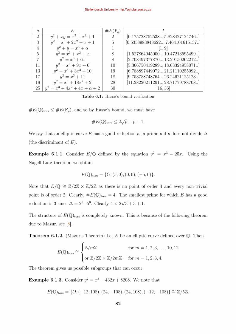
q E #E(Fq) I2 y2 + xy = x3 + x2 + 1 2 [0.175728752538.., 5.828427124746..]3 y2 = x3 + 2x2 + x+ 1 5 [0.5358983848622.., 7.464101615137..]4 y2 + y = x3 + α 1 [1, 9]5 y2 = x3 + x2 + x 8 [1.527864045000.., 10.47213595499..]7 y2 = x3 + 6x 8 [2.708497377870.., 13.29150262212..]11 y2 = x3 + 9x+ 6 10 [5.366750419289.., 18.63324958071..]13 y2 = x3 + 3x2 + 10 19 [6.788897449072.., 21.21110255092..]17 y2 = x3 + 11 18 [9.753788748764.., 26.24621125123..]19 y2 = x3 + 18x2 + 2 28 [11.28220211291.., 28.71779788708..]25 y2 = x3 + 4x2 + 4x+ α + 2 30 [16, 36]

Table 6.1: Hasse’s bound verification

#E(Q)tors ≤ #E(Fp), and so by Hasse’s bound, we must have

#E(Q)tors ≤ 2√p+ p+ 1.

We say that an elliptic curve E has a good reduction at a prime p if p does not divide ∆

(the discriminant of E).

Example 6.1.1. Consider E/Q defined by the equation y2 = x3 − 25x. Using the

Nagell-Lutz theorem, we obtain

E(Q)tors = O, (5, 0), (0, 0), (−5, 0).

Note that E/Q ∼= Z/2Z × Z/2Z as there is no point of order 4 and every non-trivial

point is of order 2. Clearly, #E(Q)tors = 4. The smallest prime for which E has a good

reduction is 3 since ∆ = 26 · 56. Clearly 4 < 2√

3 + 3 + 1.

The structure of E(Q)tors is completely known. This is because of the following theorem

due to Mazur, see [8].

Theorem 6.1.2. (Mazur’s Theorem) Let E be an elliptic curve defined over Q. Then

E(Q)tors∼=

Z/mZ for m = 1, 2, 3, . . . , 10, 12

or Z/2Z× Z/2mZ for m = 1, 2, 3, 4.

The theorem gives us possible subgroups that can occur.

Example 6.1.3. Consider y2 = x3 − 432x+ 8208. We note that

E(Q)tors = O, (−12, 108), (24,−108), (24, 108), (−12,−108) ∼= Z/5Z.

82


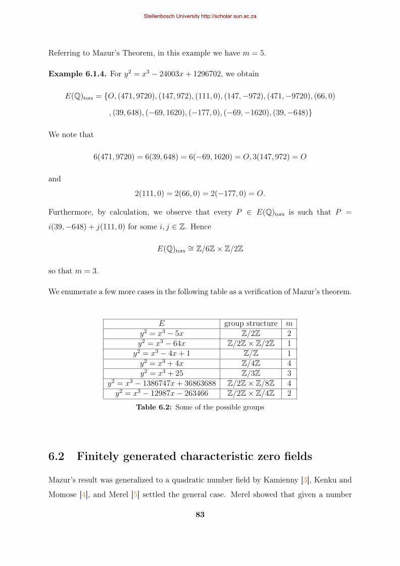
Referring to Mazur’s Theorem, in this example we have m = 5.

Example 6.1.4. For y2 = x3 − 24003x+ 1296702, we obtain

E(Q)tors = O, (471, 9720), (147, 972), (111, 0), (147,−972), (471,−9720), (66, 0)

, (39, 648), (−69, 1620), (−177, 0), (−69,−1620), (39,−648)

We note that

6(471, 9720) = 6(39, 648) = 6(−69, 1620) = O, 3(147, 972) = O

and

2(111, 0) = 2(66, 0) = 2(−177, 0) = O.

Furthermore, by calculation, we observe that every P ∈ E(Q)tors is such that P =

i(39,−648) + j(111, 0) for some i, j ∈ Z. Hence

E(Q)tors∼= Z/6Z× Z/2Z

so that m = 3.

We enumerate a few more cases in the following table as a verification of Mazur’s theorem.

E group structure my2 = x3 − 5x Z/2Z 2y2 = x3 − 64x Z/2Z× Z/2Z 1y2 = x3 − 4x+ 1 Z/Z 1y2 = x3 + 4x Z/4Z 4y2 = x3 + 25 Z/3Z 3

y2 = x3 − 1386747x+ 36863688 Z/2Z× Z/8Z 4y2 = x3 − 12987x− 263466 Z/2Z× Z/4Z 2

Table 6.2: Some of the possible groups

6.2 Finitely generated characteristic zero fields

Mazur’s result was generalized to a quadratic number field by Kamienny [3], Kenku and

Momose [4], and Merel [5] settled the general case. Merel showed that given a number

83


field of degree at most d ≥ 1, the cardinality of the torsion subgroup of an elliptic curve

defined over the number field is bounded by a constant that depends only on d. There

have been developments in trying to come up with bounds as functions of the degree of

extension to general fields other than number fields. A result by Breuer [1] expresses an

upper bound of the number of L-rational torsion points on a given elliptic curve over a

finitely generated field K as a function of the degree [L : K]. We discuss this result in

the context of elliptic curves without complex multiplication.

Throughout this section, unless otherwise specified,K is a finitely generated characteristic

zero field, Ksep is the separable closure of K in K and L is a finite extension of K. We

set GK := Gal(Ksep/K).

Definition 6.2.1. Let a be a non-zero element of Z and E an elliptic curve. The set

E[a] is called the a-torsion submodule of E and was defined already. The a-power torsion

submodule is given by E[a∞] = ∪n≥1E[an] and Etor = ∪a∈ZE[a] is called the full torsion

submodule. We also define

Etor(L) := x ∈ E : σ(x) = x ∀σ ∈ Gal(Ksep/L).

Let GK act on E[a]. After fixing a basis for E[a], one gets a Galois representation

ρa : GK → Aut(E[a]) ∼= GL2(Z/aZ).

The index of ρa(GK) is denoted by I(a), i.e

I(a) = (GL2(Z/aZ) : ρa(GK)).

Example 6.2.2. Consider an elliptic curve E : y2 = x3 + ax2 + bx + c over Q. It is

clear that E is a Z-module. Furthermore, for every m 6= 0, we have E[m] ∼= (Z/mZ)2.

Consider the field Q(x1, y1, . . . , xn, yn) = Q(E[m]) where we adjoin the coordinates of all

finite m-torsion points (xi, yi), i = 1, 2 . . . , n = m2 − 1. Fix a basis P1, P2 of E[m]. Let

σ ∈ Gal(Q(E[m])/Q). Then σ([m]P ) = [m](σ(P )),i.e the Galois action commutes with

the action of Z. For P ∈ E[m], σ(P ) is completely determined by specifying σ(P1) and

σ(P2). Suppose σ(P1) = aP1 + cP2 and σ(P2) = bP1 + dP2. We use the following matrix

notation

(σ(P1), σ(P2)) = (P1, P2)

a b

c d

.

84


Let ρm : Gal(Q(E[m])/Q)→ GL2(Z/mZ) be defined as

ρm(σ) =

a b

c d

.

A calculation shows that ρm is a homomorphism and thus a Galois representation.

We note that the coordinates of m-torsion points are algebraic and can be obtained from

polynomials called division polynomials. About division polynomials for torsion points,

refer to [10]. For instance, in Example 4.2.8, for m = 2, we needed the points (x, y) to

satisfy x3 + ax2 + bx + c = 0. For m = 3 in Example 4.2.9, to find 3-torsion points, we

needed x to satisfy 3x4 + 4ax3 + 6bx2 + 12cx+ 4ac− b2 = 0.

Lemma 6.2.3. Let d ≥ 3, t ≥ 3 and r ≥ 1 be integers. Given that d ≥ B tr

log log t, it follows

that t ≤ B′(d log log d)1/r for some constant B′ = B′(B, r), i.e B′ depends on r and the

constant B.

Proof. If d ≥ B tr

log log t, i.e d ≥ ( B

log log t)tr, then we can find a constant Bh with h > 0

such that d ≥ Bhtr−h. Here, Bh means that the constant depends on h. Then we have

d/Bh ≥ tr−h ⇒ log log(d/Bh) ≥ log log(tr−h) = log(r − h) + log log t, i.e log log(d/Bh)−

log(r− h) ≥ log log t. Thus log log t ≤ log log(d/Bh) ≤ B′′ log log d for some constant B′′.

From the hypothesis condition, we must have tr ≤ 1Bd log log t so that tr ≤ B′′

Bd log log d

and the result follows.

Lemma 6.2.4. Let K1 and K2 be fields. The compositum of the fields Ki’s, for i = 1, 2

is denoted by K1K2. Let Ki/K and Li/Ki be finite extensions in K, i = 1, 2. Then

[K1 : K][K2 : K]

[K1K2 : K]≤ [L1 : K][L2 : K]

[L1L2 : K].

Proof. By definition, L1L2 is the smallest field containing both L1 and L2, and the same

applies to K1K2. So we must have

[L1 : K1][L2 : K2] ≥ [L1L2 : K]

[K1K2 : K],

i.e[L1 : K1][L2 : K2]

[L1L2 : K]≥ 1

[K1K2 : K]

85


But

[L1 : K1] =[L1 : K]

[K1 : K]and [L2 : K2] =

[L2 : K]

[K2 : K]

so that[L1 : K][L2 : K]

[K1 : K][K2 : K]

1

[L1L2 : K]≥ 1

[K1K2 : K],

and the result follows.

Let T ⊂ E[a] where a is a non-zero integer. We set FixAut(E[a])(T ) = σ ∈ Aut(E[a]) :

σ(t) = t ∀ t ∈ T and denote the fixed field of ρ−1a (FixAut(E[a])(T )) by K(T ).

Lemma 6.2.5.

[K(T ) : K] =(ρa(GK) : ρa(GK) ∩ FixAut(E[a])(T )

).

When T = x, we write K(T ) = K(x).

Proof. See [1].

Let a be a non-zero integer. We define |a| := |Z/aZ| and

β(a) =∏p|a

(1− 1

p

)−1

in which the product ranges over all prime factors of a.

Lemma 6.2.6. Let a ∈ Z be non-zero. Then β(a) ≤ B log log |a|. Furthermore, if

an =∏

p≤n p holds, then β(an) ≥ B′ log log |a| for all n ∈ N. In either case, B and B′ are

absolute constants.

Proof. See [1]

Lemma 6.2.7. Let p be a prime integer and n be an integer greater than or equal to 1.

Then we have the exact sequence

1→ 1 + A2(pZ/pnZ)→ GL2(Z/pnZ)→ GL2(Z/pZ)→ 1

where A2 denotes the additive group of 2× 2 matrices.

86


Proof. Let A ∈ 1 + A2(pZ/pnZ). Then det(A) = 1 + y where y ∈ pZ/pnZ. Note that

(Z/pnZ)/(pZ/pnZ) ∼= Z/pZ, which is a field. Furthermore, any ideal of Z/pnZ is of

the form bZ/pnZ where bZ is an ideal of Z with pnZ ⊆ bZ, i.e b|pn. Thus we have

bZ = pkZ, k = 1, . . . , n and so it follows that Z/pnZ is a local ring with the maximal

ideal pZ/pnZ. Since det(A) ≡ 1 mod (pZ/pnZ), i.e det(A) /∈ pZ/pnZ which implies

that det(A) is a unit in Z/pnZ. So we have the natural inclusion 1 + A2(pZ/pnZ) ⊂

GL2(Z/pnZ). We claim that the map (xij + pnZ) → (xij + pZ) is a surjective homo-

morphism from GL2(Z/pnZ) onto GL2(Z/pZ). This is because given (xij + pZ) with

det(xij) /∈ pZ, then det(xij + pnZ) /∈ pZ/pnZ. The fact that pZ/pnZ is the unique

maximal ideal of Z/pnZ implies that det(xij + pnZ) is a unit in Z/pnZ.

Lemma 6.2.8. For a non-zero integer a, we have

|GL2(Z/aZ)| = |a|4∏p|a

(1− 1

p

)(1− 1

p2

)where the product ranges over the prime factors of a.

Proof. Without loss of generality, we can assume that a > 0. Then a = pr11 pr22 . . . prmm for

some prime integers p1, p2, . . . , pm. Thus

Z/aZ ∼= Z/pr11 Z× Z/pr22 Z× . . .× Z/prmm Z

by the Chinese Remainder theorem. So we have

(Z/aZ)2 ∼= (Z/pr11 Z)2 × (Z/pr22 Z)2 × . . .× (Z/prmm Z)2

which implies that

GL2(Z/aZ) ∼= GL2(Z/pr11 Z)×GL2(Z/pr22 Z)× . . .×GL2(Z/prmm Z).

Thus GL2(Z/aZ) is multiplicative in a. It is enough to show the result for a = pn where

p is a prime integer. The ring Z/pZ is a finite field containing p elements. In such case,

from the theory of automorphism groups of vector spaces over finite fields, we know that

GL2(Z/pZ) = (p2 − 1)(p2 − p).

Then from the exact sequence in Lemma 6.2.7, we have

GL2(Z/pnZ)/(1 + A2(pZ/pnZ)) ∼= GL2(Z/pZ)

87


so that

|GL2(Z/pnZ)| = |pZ/pnZ|4|GL2(Z/pZ)|

= p4(n−1)p4

(1− 1

p

)(1− 1

p2

)= p4n

(1− 1

p

)(1− 1

p2

).

Lemma 6.2.9. Let F and H be subgroups of a finite group G. Then (F : F ∩H) ≤ (G :

H).

Proof. Define a map φ : F × H → G by (f, h) 7→ fh. Let f1h1 = f2h2. Then f−12 f1 =

h2h−11 = x ∈ F ∩H so that f1 = f2x and h1 = x−1h2. i.e (f1, h1) = (f2x, x

−1h2). So for

a fixed g ∈ φ(F ×H), we have

|t ∈ F ×H : φ(t) = g| = |F ∩H|.

Hence|F ×H||F ∩H|

= |φ(F ×H)| ≤ |G|

which implies that|F ||F ∩H|

≤ |G||H|

.

Proposition 6.2.10. Let x ∈ Etor have order a. It follows that

[K(x) : K] =1

δa2∏p|a

(1− 1

p2

)

where δ ∈ [1, I(a)].

Proof. Choosing a basis for E[a] such that x is the first basis element, we see that J ∈

FixAut(E[a])(x) if and only if Jx = x, i.e J is of the form J = (aij), aij ∈ Z/aZ, 1 ≤ i, j ≤ 2

with a11 = 1, a21 = 0 and a22 ∈ GL1(Z/aZ), i.e a22 is a unit in Z/aZ. Since we can choose

a12 ∈ Z/aZ arbitrary, we thus have

|FixAut(E[a])(x)| = a|GL1(Z/aZ)|.

88


Using Lemma 6.2.8, we have

|FixAut(E[a])(x)| = a2∏p|a

(1− 1

p

)Let T = x in Lemma 6.2.5. Then

[K(x) : K] =|ρa(GK)|

|ρa(GK) ∩ FixAut(E[a])(x)|

=|GL2(Z/aZ)|

I(a)·(FixAut(E[a])(x) : FixAut(E[a])(x) ∩ ρa(GK)

)|FixAut(E[a])(x)|

=

(I(a)(

FixAut(E[a])(x) : FixAut(E[a])(x) ∩ ρa(GK)))−1

· |GL2(Z/aZ)||FixAut(E[a])(x)|

It is clear that (FixAut(E[a])(x) : FixAut(E[a])(x) ∩ ρa(GK)

)≥ 1

which implies that

I(a)(FixAut(E[a])(x) : FixAut(E[a])(x) ∩ ρa(GK)

) ≤ I(a).

On the other hand, setting F = FixAut(E[a])(x), H = ρa(GK) and G = GL2(Z/aZ) in

Lemma 6.2.9 yields the inequality

(FixAut(E[a])(x) : FixAut(E[a])(x) ∩ ρa(GK)

)≤ I(a)

so thatI(a)(

FixAut(E[a])(x) : FixAut(E[a])(x) ∩ ρa(GK)) ≥ 1

and the result holds by setting δ = I(a)

(FixAut(E[a])(x):FixAut(E[a])(x)∩ρa(GK))and using Lemma

6.2.8.

Recall the zeta-function on Z, ζ(s) =∏

p (1− p−s)−1 where the product ranges over all

prime integers.

Proposition 6.2.11. Let a be a non-zero integer and x1, x2 ∈ E[a] be a basis. Then

there is a constant C such that∏2i=1[K(xi) : K]

[K(E[a]) : K]≤ Cβ(a)

and C depends on I(a).

89


Proof. Let T = E[a] in Lemma 6.2.5. Then FixAut(E[a])(E[a]) = 1 so that

[K(E[a]) : K] = |ρa(GK)| = 1

I(a)|GL2(Z/aZ)|.

Using Lemma 6.2.8 and Proposition 6.2.10, we have∏2i=1[K(xi) : K]

[K(E[a]) : K]=I(a)

∏2i=1[K(xi) : K]

|GL2(Z/aZ)|

≤I(a)

∏2i=1

(|a|2

∏p|a

(1− 1

p2

))|GL2(Z/aZ)|

=I(a)|a|4

∏2i=1

∏p|a

(1− 1

p2

)|a|4

∏p|a

(1− 1

p

)(1− 1

p2

)= I(a)

∏p|a

(1− 1

p

)−1(1− 1

p2

)

≤ I(a)∏p|a

(1− 1

p

)−1

= I(a)β(a).

Lemma 6.2.12. Let a and b be non-zero integers such that b|a. Then I(b) ≤ I(a).

Proof. Let θ : GL2(Z/aZ) → GL2(Z/bZ) be defined as (xij) 7→ (xij mod b). Note that

θ is well defined since det(xij) ∈ (Z/aZ)× ⇒ det(xij) ∈ (Z/bZ)×. We also note that

ker θ = g ∈ GL2(Z/aZ) : g ≡ 1 mod b where 1 is the identity matrix. Denote by θ

the restriction of θ to ρa(GK). Clearly ρb(GK) = θ(ρa(GK)) and ker θ = ker θ ∩ ρa(GK)

which implies that|ρa(GK)|

|ker θ ∩ ρa(GK)|= |ρb(GK)|.

Recall that

I(b) =|GL2(Z/bZ)||ρb(GK)|

=|GL2(Z/bZ)| · |ker θ ∩ ρa(GK)|

|ρa(GK)|

=|GL2(Z/aZ)| · |ker θ ∩ ρa(GK)|

|ρa(GK)||ker θ|

90


and

I(a) =|GL2(Z/aZ)||ρa(GK)|

.

Calculation shows that

I(b)

I(a)=|ker θ ∩ ρa(GK)|

|ker θ|≤ 1⇒ I(b) ≤ I(a).

Theorem 6.2.13. Let E be an elliptic curve over K without complex multiplication.

Then

a. There is a constant C depending on E and K so that for any finite extension L/K,

|Etors(L)| ≤ C([L : K] log log[L : K])1/2.

a. Consider a prime integer p. There is a constant C depending on E, K and p such

that for every finite extension L/K,

|E[p∞](L)| ≤ C[L : K]1/2.

Proof. Recall that GK acts on E[a], giving a Galois representation

ρa : GK → Aut(E[a]) ∼= GL2(Z/aZ).

The index I(a) = (GL2(Z/aZ) : ρa(GK)) is bounded independently of a. This is due to

Serre [6].

Let T = Etors(L) and a be the smallest positive integer for which T ⊂ E[a]. Choose a

basis x1, x2 of E[a] with the property that T is generated by yi’s with yi ∈ 〈xi〉 and yi

is of order ai where i = 1, 2. Thus K(T ) =∏2

i=1K(yi). By Lemma 6.2.4, Proposition

6.2.11 and Lemma 6.2.6, we have∏2i=1[K(yi) : K]

[K(T ) : K]≤∏2

i=1[K(xi) : K]

[K(E[a]) : K]

≤ B1β(a) ≤ B2 log log a

91


where B2 does not depend on T . Using Proposition 6.2.10, we have

[K(T ) : K] ≥∏2

i=1[K(yi) : K]

B2 log log a

≥ 1

(B2 log log a)∏2

i=1 δi

2∏i=1

∏p|ai

(1− 1

p2

)a2

1a22 where 1 ≤ δi ≤ I(ai)

≥ 1

(B2 log log a)∏2

i=1 I(ai)

2∏i=1

∏p|ai

(1− 1

p2

)a2

1a22

≥ 1

(B2 log log a)∏2

i=1 I(ai)·

2∏i=1

1∏p

(1− 1

p2

)−1

· a21a

22

≥ 1

I(a)2ζ(2)2· a2

1a22

B2 log log asince I(ai) ≤ I(a) for all i.

≥ B3|T |2

log log |T |

where B3 is a constant that neither depends on T nor I(a).

Now (a) follows from Lemma 6.2.3 by setting t = |T |, r = 2 and d = [K(T ) : K].

Furthermore, if T = E[p∞], then a = pn for some n ∈ N. But β(pn) = (1 − p−1)−1

which depends only on p and so log log |T | is a constant that depends on p. Thus part

(b) follows.

The theorem gives an upper bound on the cardinality of the torsion subgroup with coor-

dinates in a specified extension.

92


Chapter 7

Applications of elliptic curves


Elliptic curves have several applications. Some of the known applications occur in cryp-

tography and we will discuss them in this chapter.

7.1 Diffie-Hellman Key Exchange

Given an elliptic curve E defined over a finite field. Let P be a non-trivial point and

Q ∈ 〈P 〉. The elliptic curve discrete logarithm problem (ECDLP) seeks to find an integer

x such that xP = Q. Generally, it is difficult to efficiently solve this problem if the sought

integer x is very large. Cryptosystems built based on the ECDLP are secure as long as

one does not find such an x very easily. One such cryptosystem is the Diffie-Helmann key

exchange in which two people exchange a private key that will be used for later commu-

nication. We will call the two parties communicating Alice and Bob. The stages in the

key exchange are highlighted below.

The shared key Ks is computed to be the first coordinate of nbCa. If Alice and Bob

are to communicate safely using their newly shared private key, then they have to make

sure that na and nb are kept secret. Thus an ‘enemy’ who presumably knows Ca and Cb

will have to solve the ECDLP mP = Ca or wP = Cb and extract the key from mCb or

wCa, respectively. To see why this is true, note that mP = naP so that m ≡ na + kr for

some integer r, and k = |〈P 〉|. Hence mCb = (na + kr)Cb = nanbP from which Ks can

93


Diffie-Hellman key exchange1. Public parameter creation

A trusted party publishes a large prime p, an elliptic curve E defined over Fpand a point P ∈ E(Fp).2. Private computations

Alice chooses a secret integer na and computes Ca = naP .Bob chooses a secret integer nb and computes Cb = nbP .

3. Value exchangeBob sends to Alice Cb and Alice sends to Bob Ca.

4. Key computationAlice computes naCb = nanbP and Bob computes nbCa = nbnaP .

be extracted. The other case is similar.

There are various tools for solving ECDLP in certain cases. But in general, it still remains

a difficult problem.

Example 7.1.1. Suppose that the trusted authority publishes E : y2 = x3 + 1000x+ 16,

p = 1000117 and P = (0, 4). Assume that Alice and Bob choose their secret integers na =

189 and nb = 157, respectively. Then Ca = (586177, 754447) and Cb = (205963, 547583).

Thus naCb = 189(205963, 547583) = 157(586177, 754447) = (872536, 465976). So their

shared key Ks = 872536 which they can use for communication.

7.2 Integer factorisation

The RSA cryptosystem, which is based on the difficulty to factorise a composite integer,

is unsafe if a highly efficient algorithm can be found for integer factorization. A number

of methods have been developed to factor integers. One of them uses elliptic curves. The

method is called Lenstra’s method. We will present the idea behind this method and

implement it in SAGE with some modification.

For simplicity, assume we want to factor a large composite integer n which is a product

of two primes p and q.

We consider an elliptic curve E mod n. Let P be a point on this curve. In trying to

compute 2P , we first find the gradient of the tangent line at P . Let d be the denominator

of the gradient we are computing. If d−1 mod n exists, then we proceed. Otherwise,

gcd(d, n) 6= 1 and so we have found a factor of n. If we are lucky, this factor may be

94


non-trivial. The algorithm is provided below. For specific technical details, refer to [10].

Elliptic curve factorisation

1. Choose an elliptic curve E mod n at random and a point P on E.

2. Choose an integer B and try to compute (B!)P .

3. If (2) fails at some point, then we have found a factor of n.

4. If (2) succeeds, then increase B or use a different elliptic curve and repeat the process.

Definition 7.2.1. Let n and B be a positive integers. Consider the prime factorisation

n = pα11 p

α22 . . . pαmm . Then n is called B-smooth if pi ≤ B for all i.

The reason for B! in the above algorithm is that if we choose several random elliptic

curves E, probably one of them will have a point P whose order is B-smooth and thus

(B!)P = O. So, at this stage we may find our factors. Note that if n is B-smooth, then

all its distinct prime factors divide B! .

In practice B is chosen to be around 108.

Example 7.2.2. Suppose we would like to factor 35. Consider the curve y2 = x3−20x+

21. An easy calculation shows that P = (15,−4) is a point on E. Let us try B = 20. We

have the following computations.

The gradient, λ, at P is 3(15)2−20−8

= 65527

. Thus d = 27 and d−1 ≡ 13 mod 35 so that λ =

8515 = 10. Now 2P = (x, y) is such that x = 102− 30 = 0 and y = −10(0− 15) + 4 = 14.

So 2P = (0, 14). We now compute 3P = 2P + P . Here, λ = 14+4−15

= 715. We note that

15−1 does not exist mod 35. So we have found a factor! This factor is gcd(15, 35) = 5

and so the other factor is just 355

= 7.

The example above shows the existence of situations where B may not play its role.

However, we cannot tell in advance whether setting B will be relevant or not.

95


We therefore propose an implementation of the algorithm in which B is not taken into

consideration. The implementation is based on SAGE syntax as shown in the Appendix,

item 3. Here is the description of the program.

We assume the input n is a positive integer made up of two distinct primes (though

we can as well consider the arbitrary case). The program creates an elliptic curve curve

of the form y2 + ax+ a2 where a ∈ Z/nZ. So we work on this elliptic curve mod n. Then

the program creates a point P = (0, a) on the curve. It computes 2P, 3P, 4P, . . .. In the

process of computing the points, at each stage of computing the gradient, it computes

the greatest common divisor (gcd) of the denominator and n. If the gcd is equal to n,

then it creates a new curve and a new point on this curve. If the gcd is equal to 1, it

proceeds computing the gradient. If none of the above cases occurs, then a non-trivial

factor has been found, and the program computes a factor of n by calculating the gcd of

n and the denominator of the gradient at that stage. The program stops only when a

non-trivial factor has been found.

96


Chapter 8

Conclusion

Elliptic curves are indeed an interesting class of algebraic curves. From the definition of

their group law, we notice the interplay between geometry and algebra. Such a curve can

be realised as a non-singular cubic equation with at least a point on it. This makes the

study of elliptic curves better as we are reduced to the case of cubic equations. When

defined over various fields, results for elliptic curves vary. For instance, when the base field

is finite, we have seen that exact formulae for the size of points with specified coordinates

can be derived. On the other hand, if the base field is not finite, you can have infinite or

finite size and the structure of the torsion subgroup can be complicated in general.

We have noted that complex elliptic curves are the same as tori. This helps us understand

the structure of the m-torsion subgroups and such a structure can be made more precise.

A proof of the Nagell-Lutz theorem using formal groups has been presented as opposed

to using detailed explicit computations that involve transforming the origin to a finite

point and working with the new equation. Of course that required deriving the formal

group associated to an elliptic curve. The Nagell-Lutz theorem is one of the important

theorems if the torsion subgroup for elliptic curves defined over Q is sought. This is

because it gives an algorithm for computing torsion points in finitely many steps. A

survey of some general results on torsion points has been made and several examples given

in order to verify the results. Of great importance is the fact that elliptic curves have

several practical applications. An area of cryptography called elliptic curve cryptography

is devoted to studying such applications. In this thesis, we only presented two amongst

the many applications which are known. Thus one can factor integers as well as do a

97


key exchange. We implemented Lenstra’s elliptic curve factorisation without taking into

account the smoothness property. This consideration was done in a hope that we may

still be able to factorize integers.

98


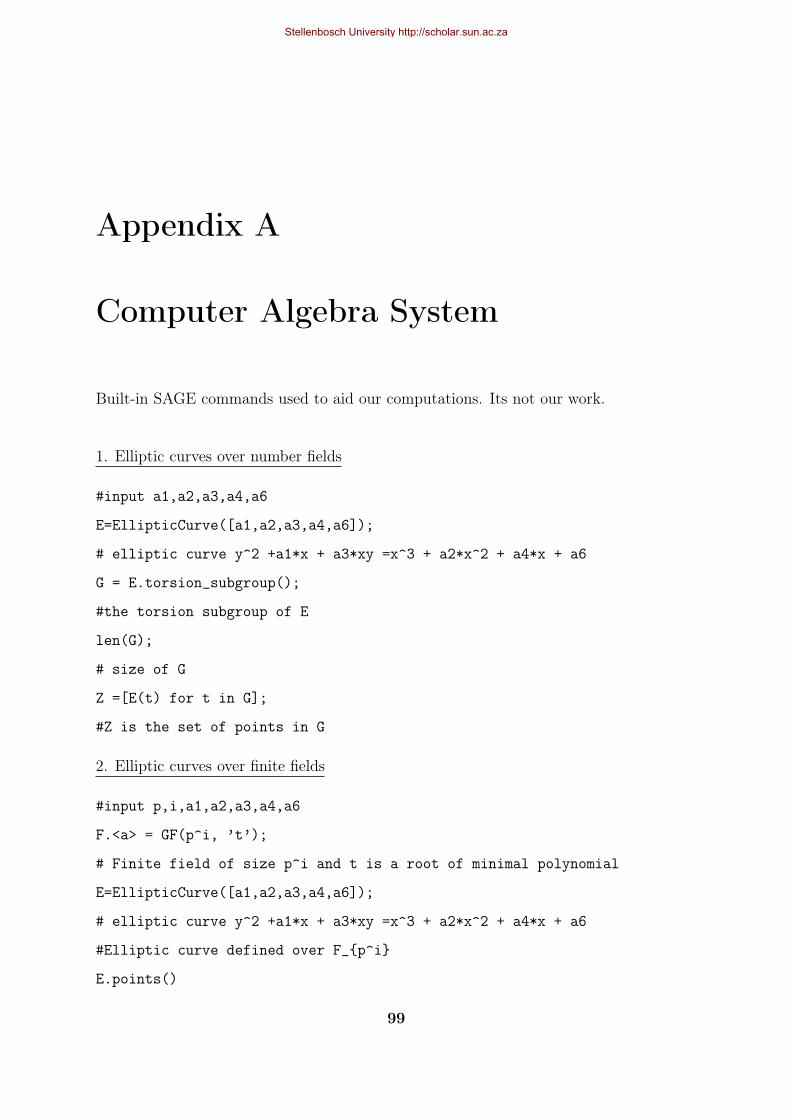
Appendix A

Computer Algebra System

Built-in SAGE commands used to aid our computations. Its not our work.

1. Elliptic curves over number fields

#input a1,a2,a3,a4,a6

E=EllipticCurve([a1,a2,a3,a4,a6]);

# elliptic curve y^2 +a1*x + a3*xy =x^3 + a2*x^2 + a4*x + a6

G = E.torsion_subgroup();

#the torsion subgroup of E

len(G);

# size of G

Z =[E(t) for t in G];

#Z is the set of points in G

2. Elliptic curves over finite fields

#input p,i,a1,a2,a3,a4,a6

F.<a> = GF(pî, ’t’);

# Finite field of size pî and t is a root of minimal polynomial

E=EllipticCurve([a1,a2,a3,a4,a6]);

# elliptic curve y^2 +a1*x + a3*xy =x^3 + a2*x^2 + a4*x + a6

#Elliptic curve defined over F_pî

E.points()

99


#List of points on E

100


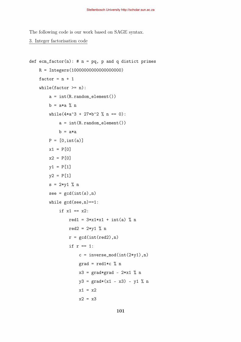
The following code is our work based on SAGE syntax.

3. Integer factorisation code

def ecm_factor(n): # n = pq, p and q distict primes

R = Integers(10000000000000000000)

factor = n + 1

while(factor >= n):

a = int(R.random_element())

b = a*a % n

while(4*a^3 + 27*b^2 % n == 0):

a = int(R.random_element())

b = a*a

P = [0,int(a)]

x1 = P[0]

x2 = P[0]

y1 = P[1]

y2 = P[1]

s = 2*y1 % n

see = gcd(int(s),n)

while gcd(see,n)==1:

if x1 == x2:

red1 = 3*x1*x1 + int(a) % n

red2 = 2*y1 % n

r = gcd(int(red2),n)

if r == 1:

c = inverse_mod(int(2*y1),n)

grad = red1*c % n

x3 = grad*grad - 2*x1 % n

y3 = grad*(x1 - x3) - y1 % n

x1 = x2

x2 = x3

101


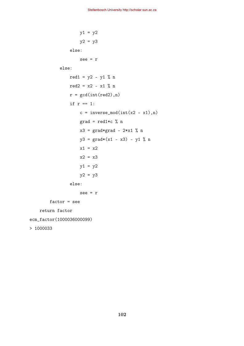
y1 = y2

y2 = y3

else:

see = r

else:

red1 = y2 - y1 % n

red2 = x2 - x1 % n

r = gcd(int(red2),n)

if r == 1:

c = inverse_mod(int(x2 - x1),n)

grad = red1*c % n

x3 = grad*grad - 2*x1 % n

y3 = grad*(x1 - x3) - y1 % n

x1 = x2

x2 = x3

y1 = y2

y2 = y3

else:

see = r

factor = see

return factor

ecm_factor(1000036000099)

> 1000033

102


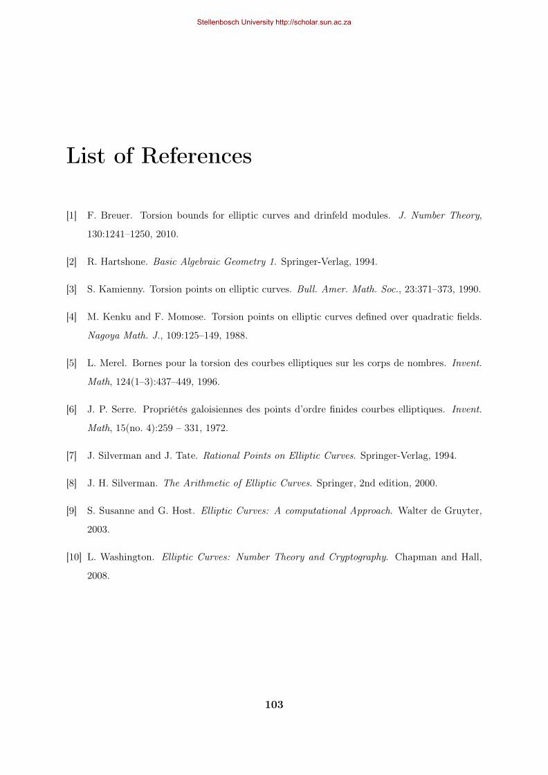
List of References

[1] F. Breuer. Torsion bounds for elliptic curves and drinfeld modules. J. Number Theory,

130:1241–1250, 2010.

[2] R. Hartshone. Basic Algebraic Geometry 1. Springer-Verlag, 1994.

[3] S. Kamienny. Torsion points on elliptic curves. Bull. Amer. Math. Soc., 23:371–373, 1990.

[4] M. Kenku and F. Momose. Torsion points on elliptic curves defined over quadratic fields.

Nagoya Math. J., 109:125–149, 1988.

[5] L. Merel. Bornes pour la torsion des courbes elliptiques sur les corps de nombres. Invent.

Math, 124(1–3):437–449, 1996.

[6] J. P. Serre. Propriétés galoisiennes des points d’ordre finides courbes elliptiques. Invent.

Math, 15(no. 4):259 – 331, 1972.

[7] J. Silverman and J. Tate. Rational Points on Elliptic Curves. Springer-Verlag, 1994.

[8] J. H. Silverman. The Arithmetic of Elliptic Curves. Springer, 2nd edition, 2000.

[9] S. Susanne and G. Host. Elliptic Curves: A computational Approach. Walter de Gruyter,

2003.

[10] L. Washington. Elliptic Curves: Number Theory and Cryptography. Chapman and Hall,

2008.

103


Torsion Points on Elliptic curves

Documents

Transcript of Torsion Points on Elliptic curves