
Topology of the space of metrics with positive scalar ... · Topology of the space of metrics with...
36
Topology of the space of metrics with positive scalar curvature Boris Botvinnik University of Oregon, USA March 12, 2016 Shanks Workshop on Geometric Analysis Vanderbilt University
Transcript of Topology of the space of metrics with positive scalar ... · Topology of the space of metrics with...

Topology of the space of metrics with positive
scalar curvature
Boris BotvinnikUniversity of Oregon, USA
March 12, 2016
Shanks Workshop on Geometric Analysis
Vanderbilt University
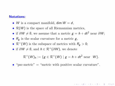
Notations:
• W is a compact manifold, dimW = d ,
• R(W ) is the space of all Riemannian metrics,
• if @W 6= ;, we assume that a metric g = h + dt2 near @W ;
• Rg is the scalar curvature for a metric g ,
• R+(W ) is the subspace of metrics with Rg > 0;
• if @W 6= ;, and h 2 R+(@W ), we denote
R+(W )h := {g 2 R+(W ) | g = h + dt2 near W }.
• “psc-metric” = “metric with positive scalar curvature”.

Existence Question:
• For which manifolds W the space R+(W ) is not empty?
It is well-known that for a closed manifold W ,
R+(W ) 6= ; () Y (W ) > 0.
Yamabe invariant��
Assume R+(W ) 6= ;.
More Questions:
• What is a topology of R+(W )?
• In particular, what are the homotopy groups ⇡kR+(W )?

Let (W , g) be a spin manifold. Then there is a canonical realspinor bundle Sg ! W and a Dirac operator Dg acting on thespace L2(W , Sg ).
Theorem. (Lichnerowicz ’60)D2g = �s
g + 14Rg . In particular, if Rg > 0 then Dg is invertible.
For a spin manifold W , dimW = d , we obtain a map
(W , g) 7! DgqD2g + 1
2 Fredd ,0,
where Fredd ,0 is the space of C`d -linear Fredholm operators.
The space Fredd ,0 also classifies the real K -theory, i.e.,
⇡qFredd ,0 = KOd+q

It gives the index map
↵ : (W , g) 7! ind(Dg ) = [Dg ] 2 ⇡0Fredd ,0 = KOd .
The index ind(Dg ) does not depend on a metric g .
Index Theory gives a map:
↵ : ⌦Spind �! KOd .
Thus ↵(M) := ind(Dg ) gives a topological obstruction toadmitting a psc-metric.
Theorem. (Gromov-Lawson ’80, Stolz ’93) Let W be a spinsimply connected closed manifold with d = dimW � 5. ThenR+(W ) 6= ; if and only if ↵(W ) = 0 in KOd .
Topology: There are enough examples of psc-manifolds togenerate Ker ↵ ⇢ ⌦Spin
d , then we use surgery.

Surgery. Let W be a closed manifold, and Sp ⇥ Dq+1 ⇢ W .
We denote by W 0 the manifold which is the result of a surgeryalong the sphere Sp:
W 0 = (W \ (Sp ⇥ Dq+1)) [Sp⇥Sq (Dp+1 ⇥ Sq).
Codimension of this surgery is q + 1.
Sp⇥Dq+1⇥I1
Sp⇥Dq+2+
VV0W ⇥ I0
Dp+1⇥Dq+1
W 0W
W ⇥ I0

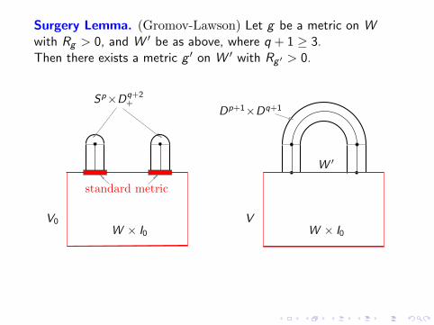
Surgery Lemma. (Gromov-Lawson) Let g be a metric on Wwith Rg > 0, and W 0 be as above, where q + 1 � 3.Then there exists a metric g 0 on W 0 with Rg 0 > 0.
g + dt2
Sp⇥Dq+2+
VV0W ⇥ I0
Dp+1⇥Dq+1
W 0W
W ⇥ I0
Surgery Lemma. (Gromov-Lawson) Let g be a metric on Wwith Rg > 0, and W 0 be as above, where q + 1 � 3.Then there exists a metric g 0 on W 0 with Rg 0 > 0.
standard metric
Sp⇥Dq+2+
VV0W ⇥ I0
Dp+1⇥Dq+1
W 0W
W ⇥ I0

Surgery Lemma. (Gromov-Lawson) Let g be a metric on Wwith Rg > 0, and W 0 be as above, where q + 1 � 3.Then there exists a metric g 0 on W 0 with Rg 0 > 0.
Sp⇥Dq+2+
VV0W ⇥ I0
Dp+1⇥Dq+1
W 0W
W ⇥ I0

Surgery Lemma. (Gromov-Lawson) Let g be a metric on Wwith Rg > 0, and W 0 be as above, where q + 1 � 3.Then there exists a metric g 0 on W 0 with Rg 0 > 0.
VV0W ⇥ I0
Dp+1⇥Dq+1
(W 0, g 0)
W
W ⇥ I0
(W , g)

Conclusion: Let W and W 0 be simply connected cobordant spinmanifolds, dimW = dimW 0 = d � 5. Then
R+(W ) 6= ; () R+(W 0) 6= ;.
Assume R+(W ) 6= ;.
Theorem. (Chernysh, Walsh) Let W and W 0 be simplyconnected cobordant spin manifolds, dimW = dimW 0 � 5. Then
R+(W ) ⇠= R+(W 0).
Let @W = @W 0 6= ;, and h 2 R+(@W ), then
R+(W )h ⇠= R+(W 0)h.
Questions:
• What is a topology of R+(W )?
• In particular, what are the homotopy groups ⇡kR+(W )?

Example. Let us show that Z ⇢ ⇡0R+(S7).
Let B be a Bott manifold, i.e. B is a simply connected spinmanifold, dimB = 8, with ↵(B8) = A(B) = 1.
Let B := B \ (D81 t D8
2 ):
B(S7, g0)(S7, g1)
Thus Z ⇢ ⇡0R+(S7).

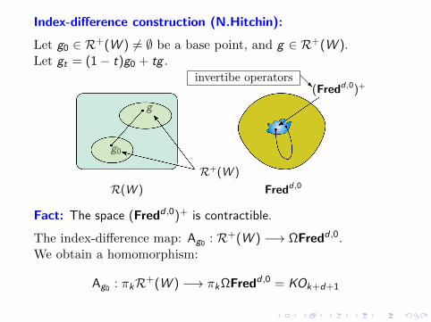
Index-di↵erence construction (N.Hitchin):
Let g0 2 R+(W ) 6= ; be a base point, and g 2 R+(W ).Let gt = (1� t)g0 + tg .
g
g0
R(W )
R+(W )
Fredd,0
(Fredd,0)+invertibe operators @R
Fact: The space (Fredd ,0)+ is contractible.
The index-di↵erence map: Ag0 : R+(W ) �! ⌦Fredd ,0.We obtain a homomorphism:
Ag0 : ⇡kR+(W ) �! ⇡k⌦Fredd ,0 = KOk+d+1

There is another way to construct the index-di↵erence map.
Let g0 2 R+(W ) 6= ; be a base point, and g 2 R+(W ), and
gt = (1� t)g0 + tg .
Then we have a cylinder W ⇥ I with the metric g = gt + dt2:
g0 gg = gt + dt2
W ⇥ I
It gives the Dirac operator Dg with the Atyiah-Singer-Patodiboundary condition. We obtain the second map
indg0 : R+(W ) �! ⌦Fredd ,0, g 7! DgqD2
g+12 Fredd+1,0 ⇠ ⌦Fredd ,0.
Index Theory: indg0 ⇠ Ag0 .
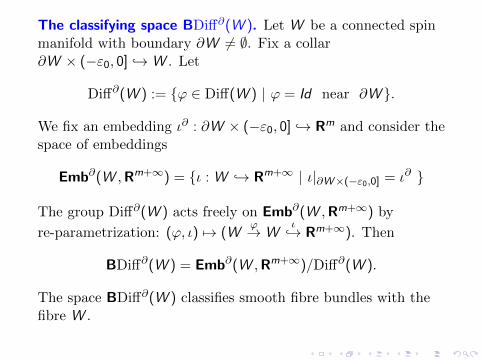
The classifying space BDi↵@(W ). Let W be a connected spinmanifold with boundary @W 6= ;. Fix a collar@W ⇥ (�"0, 0] ,! W . Let
Di↵@(W ) := {' 2 Di↵(W ) | ' = Id near @W }.
We fix an embedding ◆@ : @W ⇥ (�"0, 0] ,! Rm and consider thespace of embeddings
Emb@(W ,Rm+1) = {◆ : W ,! Rm+1 | ◆|@W⇥(�"0,0] = ◆@ }
The group Di↵@(W ) acts freely on Emb@(W ,Rm+1) by
re-parametrization: (', ◆) 7! (W'! W
◆,! Rm+1). Then
BDi↵@(W ) = Emb@(W ,Rm+1)/Di↵@(W ).
The space BDi↵@(W ) classifies smooth fibre bundles with thefibre W .
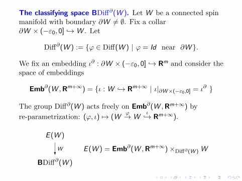
The classifying space BDi↵@(W ). Let W be a connected spinmanifold with boundary @W 6= ;. Fix a collar@W ⇥ (�"0, 0] ,! W . Let
Di↵@(W ) := {' 2 Di↵(W ) | ' = Id near @W }.
We fix an embedding ◆@ : @W ⇥ (�"0, 0] ,! Rm and consider thespace of embeddings
Emb@(W ,Rm+1) = {◆ : W ,! Rm+1 | ◆|@W⇥(�"0,0] = ◆@ }
The group Di↵@(W ) acts freely on Emb@(W ,Rm+1) by
re-parametrization: (', ◆) 7! (W'! W
◆,! Rm+1).
E (W )
BDi↵@(W )
?W E (W ) = Emb@(W ,Rm+1)⇥Di↵@(W ) W
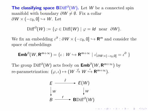
The classifying space BDi↵@(W ). Let W be a connected spinmanifold with boundary @W 6= ;. Fix a collar@W ⇥ (�"0, 0] ,! W . Let
Di↵@(W ) := {' 2 Di↵(W ) | ' = Id near @W }.
We fix an embedding ◆@ : @W ⇥ (�"0, 0] ,! Rm and consider thespace of embeddings
Emb@(W ,Rm+1) = {◆ : W ,! Rm+1 | ◆|@W⇥(�"0,0] = ◆@ }
The group Di↵@(W ) acts freely on Emb@(W ,Rm+1) by
re-parametrization: (', ◆) 7! (W'! W
◆,! Rm+1).
E E (W )
B BDi↵@(W )?W
-f
?W
-f

Moduli spaces of metrics. Let W be a connected spin manifoldwith boundary @W 6= ;, h0 2 R+(@W ). Recall:
R(W )h0 := {g 2 R(W ) | g = h0 + dt2 near @W },
Di↵@(W ) := {' 2 Di↵(W ) | ' = Id near @W }.
The group Di↵@(W ) acts freely on R(W )h0 and R+(W )h0 :
M(W )h0 = R(W )h0/Di↵@(W ) = BDi↵@(W ),
M+(W )h0 = R+(W )h0/Di↵@(W ).
Consider the map M+(W )h0 ! BDi↵@(W ) as a fibre bundle:
R+(W )h0 ! M+(W )h0 ! BDi↵@(W )

Let g0 2 R+(W )h0 be a “base point”.
We have the fibre bundle:
Let ' : I ! BDi↵@(W ) be a loop
with '(0) = '(1) = g0, and
' : I ! M+(W )h0 its lift.
M+(W )h0
BDi↵@(W )
?R+(W )h0
g0
g0
'1(g0)
't(g0)
We obtain:
g0 '1(g0)g = '1(gt) + dt2
W ⇥ I
⌦BDi↵@(W )e�! R+(W )h0
indg0�! ⌦Fredd ,0

Let W be a spin manifold, dimW = d . Consider again theindex-di↵erence map:
indg0 : R+(W ) �! ⌦Fredd ,0,where g0 2 R+(W ) is a “base-point”. In homotopy groups:
(indg0)⇤ : ⇡kR+(W ) �! ⇡k⌦Fredd ,0 = KOk+d+1.
Theorem. (BB, J. Ebert, O.Randal-Williams ’14) Let W be aspin manifold with dimW = d � 6 and g0 2 R+(W ). Then
⇡kR+(W )(indg0 )⇤����! KOk+d+1 =
8<
:
Z k + d + 1 ⌘ 0, 4 (8)Z2 k + d + 1 ⌘ 1, 2 (8)0 else
is non-zero whenever the target group is non-zero.
Remark. This extends and includes results by Hitchin (’75), byCrowley-Schick (’12), by Hanke-Schick-Steimle (’13).

Let dimW = d = 2n. Assume W is a manifold with boundary@W 6= ;, and W 0 is the result of an admissible surgery on W .For example:
W = D2n W 0 = D2n [ ((S2n�1 ⇥ I )#(Sn ⇥ Sn))
=)
Then we have:R+(D2n)h0
⇠= R+(W 0)h0 ,
where h0 is the round metric on S2n�1.
Observation: It is enough to prove the result for R+(D2n)h0 orany manifold obtained by admissible surgeries from D2n.

We need a particular sequence of surgeries:
S2n�1 S2n�1 S2n�1 S2n�1 S2n�1
V0 V1 Vk�1 Vk· · ·
Here V0 = (Sn ⇥ Sn) \ D2n,
V1 = (Sn ⇥ Sn) \ (D2n� t D2n
+ ), . . . ,Vk = (Sn ⇥ Sn) \ (D2n� t D2n
+ ).
Then Wk := V0 [ V1 [ · · · [ Vk = #k(Sn ⇥ Sn) \ D2n.
We choose psc-metrics gj on each Vj which gives the standardround metric h0 on the boundary spheres.

We need a particular sequence of surgeries:
S2n�1 S2n�1 S2n�1 S2n�1 S2n�1
h0 h0 h0 h0 h0
(V0,g0) (V1,g1) (Vk�1,gk�1) (Vk ,gk)· · ·
Here V0 = (Sn ⇥ Sn) \ D2n,
V1 = (Sn ⇥ Sn) \ (D2n� t D2n
+ ), . . . ,Vk = (Sn ⇥ Sn) \ (D2n� t D2n
+ ).
Then Wk := V0 [ V1 [ · · · [ Vk = #k(Sn ⇥ Sn) \ D2n.
We choose psc-metrics gj on each Vj which gives the standardround metric h0 on the boundary spheres.

S2n�1 S2n�1 S2n�1 S2n�1 S2n�1
h0 h0 h0 h0 h0
(V0,g0) (V1,g1) (Vk�1,gk�1) (Vk ,gk)· · ·
A �Wk�1
� A
Wk
We have the composition map
R+(Wk�1)h0 ⇥R+(Vk)h0,h0 �! R+(Wk)h0 .
Gluing metrics along the boundary gives the map:
m : R+(Wk�1)h0 �! R+(Wk)h0 , g 7! g [ gk
Geometry: The map m : R+(Wk�1)h0 �! R+(Wk)h0 ishomotopy equivalence.

S2n�1 S2n�1 S2n�1 S2n�1 S2n�1
h0 h0 h0 h0 h0
(V0,g0) (V1,g1) (Vk�1,gk�1) (Vk ,gk)· · ·
A �Wk�1
� A
Wk
Let and s : Wk ,! Wk+1 be the inclusion.It induces the stabilization maps
Di↵@(W0) ! · · · ! Di↵@(Wk) ! Di↵@(Wk+1) ! · · ·
BDi↵@(W0) ! · · · ! BDi↵@(Wk) ! BDi↵@(Wk+1) ! · · ·
Topology-Geometry: the space BDi↵@(Wk) is the moduli spaceof all Riemannian metrics on Wk which restrict to h0 + dt2 nearthe boundary @Wk .

S2n�1 S2n�1 S2n�1 S2n�1 S2n�1
h0 h0 h0 h0 h0
(V0,g0) (V1,g1) (Vk�1,gk�1) (Vk ,gk)· · ·
A �Wk�1
� A
Wk
Let and s : Wk ,! Wk+1 be the inclusion.It gives the fiber bundles:
M+(W0)h0 M+(W1)h0 �! · · · �! M+(Wk)h0 �! · · ·
BDi↵@(W0) BDi↵@(W1) �! · · ·�! BDi↵@(Wk) �! · · ·
-
?R+(W0)h0
?R+(W0)h0
?R+(Wk )h0
-
⇠= - ⇠= - ⇠=-
with homotopy equivalent fibers R+(W0)h0⇠= · · · ⇠= R+(Wk)h0
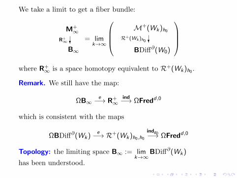
We take a limit to get a fiber bundle:
M+1
B1
?R+1 = lim
k!1
0
BB@
M+(Wk)h0
BDi↵@(W0)
?R+(Wk )h0
1
CCA
where R+1 is a space homotopy equivalent to R+(Wk)h0 .
Remark. We still have the map:
⌦B1e�! R+
1ind�! ⌦Fredd ,0
which is consistent with the maps
⌦BDi↵@(Wk)e�! R+(Wk)h0,h0
indg0�! ⌦Fredd ,0
Topology: the limiting space B1 := limk!1
BDi↵@(Wk)
has been understood.

About 10 years ago, Ib Madsen, Michael Weiss introduced newtechnique, parametrized surgery, which allows to describevarious
Moduli Spaces of Manifolds.
Theorem. (S. Galatius, O. Randal-Williams) There is a map
B1⌘�! ⌦1
0 MT✓n
inducing isomorphism in homology groups.
This gives the fibre bundles:
M+1 M+
1
B1 ⌦10 MT⇥n
-
?R+1 ?R+
1
-⌘
Again, it gives a holonomy map
e : ⌦⌦10 MT⇥n �! R+
1

The space ⌦10 MT⇥n is the moduli space of (n � 1)-connected
2n-dimensional manifolds.
In particular, there is a map (spin orientation)
↵ : ⌦10 MT⇥n �! Fred2n,0
sending a manifold W to the corresponding Dirac operator.
⌦⌦10 MT⇥n ⌦Fred2n,0
R+1
QQQse
-⌦↵
⌘⌘⌘3ind
D0 D1Dt
g0 '1(g0)'1(gt)
W ⇥ I
⌦BDi↵@(W )e�! R+(W )h0
indg0�! ⌦Fredd ,0

The space ⌦10 MT⇥n is the moduli space of (n � 1)-connected
2n-dimensional manifolds.
In particular, there is a map (spin orientation)
↵ : ⌦10 MT⇥n �! Fred2n,0
sending a manifold W to the corresponding Dirac operator.
⌦⌦10 MT⇥n ⌦Fred2n,0
R+1
QQQse
-⌦↵
⌘⌘⌘3ind
Index Theory
gives commutative
diagram
ih
Then we use algebraic topology to compute the homomorphism
(⌦↵)⇤ : ⇡k(⌦⌦10 MT⇥n) �! ⇡k(⌦Fred
2n,0) = KOk+2n+1
to show that it is nontrivial when the target group is non-trivial.
THANK YOU!


![Constant scalar curvature metrics on fibred complex surfaceshomepages.ulb.ac.be/~joelfine/thesis/thesis.pdf · Peter Gwilliam for ei ... and [Cal85] Calabi studies the functional](https://static.fdocuments.in/doc/165x107/5f45f03c6cdf0f06864228b3/constant-scalar-curvature-metrics-on-ibred-complex-joelfinethesisthesispdf.jpg)


