Topologies for Satellite Constellations in a Cross-linked ...

Topologies for Satellite Constellations in a Cross-linked

Space Backbone Network

by

Jason H. Bau

S. B., Massachusetts Institute of Technology, 200P

MASSACHUSETTS INSTITUTEOF TECHNOLOGY

JUL 3 1 2002

LIBRARIES

BARKER

Submitted to the Department of Electrical Engineering and Computer Science

in Partial Fulfillment of the Requirements for the Degree of

Master of Engineering in Electrical Engineering and Computer Science

at the

MASSACHUSETTS INSTITUTE OF TECHNOLOGY

May 20, 2002 Li 2A

@ 2002 Massachusetts Institute of Technology. All rights reserved.

AuthorDeparment of Electrical Engineering and Computer Science

May 20, 2002

Certified by-\J Vincent W. S. Chan

Joan and Irwin M. Jacob Professor of Electrical Engineering andComputer Science and Aeronautics and Astronautics

Director, Laboratory for Information and Decision SystemsT) Jhsis Supervisor

Arthur C. SmithAccepted by

Chairman, Department Committee on Graduate Theses

/

Topologies for Satellite Constellations in a Cross-linked

Space Backbone Network

by

Jason H. Bau

Submitted to the Department of Electrical Engineering and Computer Scienceon May 20, 2002, in partial fulfillment of

the requirements for the degree ofMaster of Engineering in Electrical Engineering and Computer Science

Abstract

An evolutionary space data network can be formed from satellites serving as bothbackbone and user-access nodes connected via high-speed cross-links. Such a spacebackbone network should support spacecraft-to-ground and spacecraft-to-spacecraft linksfor users of various altitudes (LEO, MEO, GEO and HEO). One main consideration inthe design of such a space network is the physical altitude and topology of the backbonesatellite constellation. In this thesis, different GEO, MEO, and LEO configurations areconsidered as backbone topologies to serve the projected user altitudes and requirements.First, exact constellations are determined for each proposed configuration that meet theuser coverage requirements while maximizing coverage efficiency. The complexities ofthese constellations are then compared using constellation parameters such as altitude, andthe number of orbital planes required, and the number of satellites required per plane, aswell as individual satellite parameters like the number of antennae required, the necessaryslewing rate of each antenna, the power required by each antenna, and the physicalplacement of these antennae on the satellites. The complexity parameters of eachindividual satellite will be determined for two of the types of communications links usedon the satellite, namely links between the user satellites and backbone satellites and linksbetween backbone satellites. These parameters are then used in a speculative cost modelto determine the cost versus complexity of each constellation. Through these calculations,a GEO backbone consisting of three satellites is determined to require a minimum numberof apertures for both types of links as well as allowing an optimal onboard placement ofthese apertures. Thus, it possesses cost vs. complexity characteristics superior to otherconstellations and should be the choice for a space-borne data backbone network.

Thesis Supervisor: Vincent W.S. ChanTitle: Joan and Jacob Professor of Electrical Engineering andComputer Science and Aeronautics and AstronauticsDirector, Laboratory for Information and Decision Systems

2

Acknowledgements

I would like to express my gratitude to all who supported me during these past

two years of graduate school. Many thanks go out to my spiritual leaders Pastor Paul,

Becky JDSN, Heechin JDSN and Scott hyung for their constant prayer and concern. I

would also like to thank my advisor Professor Chan for his patience and research guidance

and my parents for all the years of love and selfless sacrifice they gave to raise me.

Thanks also to the Concord brothers, Danny, Walter, Eddie, Austin, Eugene, Patrick,

Hero, Matt, and Orton and to the EG brothers, Thomas, Henry, Dave, Alan, and Matt

(again) for their love and patience, for putting up with my study habits, and for so many

memories. I owe you a great debt of love and a meal or two! My gratitude to all the

members of Berkland Baptist Church for being my true spiritual family. It is a privilege

for me to be related to you. To my fiancee Amy I am indebted for her constant

encouragement and urging to continue my thesis work and for supporting me in

innumerable other ways. And finally, to my Savior and my God, without whom I would

have neither life nor happiness, I can only express my eternal gratitude and offer my

devotion with all of my meager strength. I love you, Lord.

3

Table of Contents

1. Introduction and Background.............................................................................................. 11

1. 1 M otivation ..................................................................................................................... 11

1.2 Procedure ...................................................................................................................... 11

2. Projected User Requirements and Service Contract .......................................................... 13

2.1 User Requirements......................................................................................................... 13

2.2 Services Provided by Backbone Network................................................................... 13

3. Determining Candidate Constellations.............................................................................. 15

3.1 Coverage ....................................................................................................................... 15

3.2 Determination of Coverage Radius.............................................................................. 16

3.3 Polar Orbits.................................................................................................................... 18

3.4 GEO Orbit..................................................................................................................... 24

3.5 W alker LEO and M EO orbits..................................................................................... 24

4. Complexity of Backbone Links ......................................................................................... 27

4.1 Inter-Plane Links............................................................................................................ 28

4.1.1 Polar Orbits............................................................................................................. 28

4.1.2 W alker Orbits.......................................................................................................... 31

4.1.3 Slewing Rate........................................................................................................... 35

4.2 Intra-Plane Links............................................................................................................ 41

4.3 Constraint on Constellation Based on Backbone visibility ........................................... 42

4.4 Final Constellations in Study ....................................................................................... 46

5. Complexity of User-Access Links .................................................................................... 47

5.1 Upper-bound of Link Distance ..................................................................................... 47

5.2 Upper-bound of Slewing Rate ..................................................................................... 49

5.3 Number of Apertures Required for User Support ........................................................ 56

5.3.1 Effects of Geometry on Number of Apertures...................................................... 57

5.3.2 GEO Backbone.................................................................................................... 59

5.3.2.1 GEO backbone-GEO User............................................................................ 59

4

5.3.2.2 GEO backbone-M EO/LEO User .................................................................. 60

5.3.2.3 Hand-offs ................................................................................................... 64

5.3.3 E Backbone................................................................................................. 65

5.3.3.1 M EO Backbone-GEO User ........................................................................... 65

5.3.3.2 M EO Backbone-M EO/LEO User ................................................................... 70

5.3.4 LEO Backbone........................................................................................................ 73

5.3.4.1 LEO Backbone-GEO User ........................................................................... 73

5.3.4.2 LEO Backbone-M EO/LEO user ................................................................... 77

6. Cost Analysis ....................................................................................................................... 81

6.1 Cost Equation ................................................................................................................ 81

6.2 Cost Coefficients of Satellite Links.............................................................................. 82

6.3 User-Access Links ......................................................................................................... 82

6.3.1 Cost Parameters ................................................................................................... 82

6.3.2 Numerical Examples of User-Access Link Cost ................................................... 84

6.4 Intra-Backbone Links.................................................................................................. 86

6.4.1 Cost Parameters ...................................................................................................... 86

6.4.2 Numerical Examples of Intra-Backbone Link Costs ............................................. 87

6.5 Cost Equation of Entire Constellation ......................................................................... 92

6.6 Numerical Examples....................................................................................................... 93

7. Conclusions and Future Research....................................................................................... 98

References .............................................................................................................................. 101

5

List of Figures

3-1: An illustration of the coverage region .............................................................. 17

_3-2: The altitude of the backbone satellite vs. the radius of the coverage region ......... 18

3-3: An illustration for the calculation of the number of satellites required for apolar orbit to provide full coverage............................................................... 19

3-4: Parameters required for full space coverage in a polar configuration as afunction of altitude ........................................................................................ 20

3-5: The fluxes of high-energy electrons and protons in the inner Van Allen belt ........ 21

3-6: Parameters required for full terrestrial coverage in a polar configuration as afunction of altitude ........................................................................................ 23

4-1: O rbital G eom etry........................................................................................... 27

4-2: Inter-plane cross-link parameter variations vs. phase angle for P = 3, S = 4,and altitude = 1,550 km .................................................................................. 29

4-3: Inter-plane cross-link parameter variations vs. phase angle for P = 5, S = 8,and altitude = 1,550 km ................................................................................... 30

4-4: Inter-plane cross-link parameter variations vs. phase angle for P = 2, S = 3,and altitude = 15,000 km ................................................................................ 30

4-5: Inter-plane cross-link parameter variations vs. phase angle for P = 2, S = 4,and altitude = 15,000 km ................................................................................ 31

4-6: Inter-plane cross-link parameter variations vs. phase angle for Walkerconfiguration 10/5/57.1*/2, and altitude = 1,550 km......................................33

4-7: Inter-plane cross-link parameter variations vs. phase angle for Walkerconfiguration 5/5/43.70/1, and altitude = 15,000 km......................................34

4-8: Inter-plane cross-link parameter variations vs. phase angle for Walkerconfiguration 4/2/450/1, and altitude = 15,000 km...........................................34

4-9: The 1st derivatives of the elevation and azimuth angles with respect to phaseangle for the polar configuration P=3, S=4, and altitude = 1,550 km...............36

4-10: The 1V derivatives of the elevation and azimuth angles with respect to phaseangle for the polar configuration P=5, S=8, and altitude = 1,550 km ............... 36

4-11: The 1s derivatives of the elevation and azimuth angles with respect to phaseangle for the Walker configuration T/P/8/F = 10/5/57.10/2 and altitude =1,550 km ...................................................................................................... . . 37

6

4-12: The 1V derivatives of the elevation and azimuth angles with respect to phaseangle for the polar configuration P=2, S=3, and altitude = 15,000 km..............37

4-13: The 1st derivatives of the elevation and azimuth angles with respect to phaseangle for the polar configuration P=2, S=4, and altitude = 15,000 km..............38

4-14: The Vt derivatives of the elevation and azimuth angles with respect to phaseangle for the Walker configuration T/P/6/F = 5/5/43.7 '/1 and altitude =15,000 km ..................................................................................................... . 38

4-15: The 1st derivatives of the elevation and azimuth angles with respect to phaseangle for the Walker configuration T/P/6/F = 4/2/45 0/1 and altitude =15,000 km ..................................................................................................... . 39

4-16: A typical intra-backbone link ......................................................................... 41

4-17: The angle of elevation between a satellite and its tangent line to the earth.....43

4-18: An inter-plane link between S1 and S2.............................. . . . . . . . . . . . . . . . . . . . . . . . . . . . . . . 43

4-19: Inter-plane cross-link parameter variations vs. phase angle for polarconfiguration 15/5/900/1.5, and altitude = 1550 km. ....................................... 45

4-20: The Vt derivatives of the elevation and azimuth angles with respect to phaseangle for the Polar configuration T/P/6/F = 15/5/90 0/1.5 and altitude = 1550k m . .................................................................................................................... 4 5

5-1: The coverage region of S ............................................................................. 47

5-2: Calculating the maximum slewing rate in a retrograde satellite configuration.......50

5-3: A sanity check on slew rate calculations ......................................................... 52

5-4: Maximum slew rate of user-link for a LEO at 1,550 km altitude ..................... 52

5-5: Maximum slew rate of user-link for MEO backbone at 15,000 km..................53

5-6: Slewing rate vs. phase angle of user satellite of 1,500km altitude with LEObackbone at 1,550 km altitude ....................................................................... 53

5-7: A close-up of 5-6 .......................................................................................... 54

5-8: Slewing rate vs. Phase angle of user satellite with MEO backbone at 1550km altitude ..................................................................................................... 55

5-9: The overlapping coverage regions of three backbone satellites........................57

5-10: GEO backbone coverage of GEO users..........................................................59

5-11: Illustration of the coverage regions of a 3-satellite GEO backbone..................60

5-12: A GEO backbone satellite providing service to the MEO and LEO userreg io n s...............................................................................................................6 1

5-13: The coverage gap for a GEO backbone and the LEO user region.....................61

7

5-14: The projection of a GEO backbone's coverage region on the 250 km altitudeLE O user sphere ............................................................................................ 62

5-15: The visibility of the GEO orbit plane from a MEO polar orbit..........................66

5-16: Full visibility of the GEO plane from a polar MEO using only the earth-facingsurface . .............................................................................................................. 6 7

5-17: The visibility of the GEO plane from a MEO satellite 15,000 km over theeq u ato r...............................................................................................................6 8

5-18: The coverage profile of the MEO constellation on the GEO user orbit............70

5-19: A rectangular projection of the coverage profile of one plane of the MEObackbone on the 250 km LEO sphere. ................................................................ 71

5-20: The visibility of the GEO orbit plane from a LEO polar orbit..............73

5-21: Service region provided on the GEO user orbit by a LEO backbone satelliteusing only its earth-facing surface...................................................................74

5-22: The coverage region of a single LEO backbone satellite experiencingobscuration from the earth on the GEO user orbit...............................................76

5-23: A designed coverage profile of the LEO backbone constellation on the GEOu ser o rb it............................................................................................................7 6

5-24: The six nearest neighbors of satellite So. ......................................................... 78

5-25: The service area of a LEO backbone satellite on the MEO and LEO userspheres...............................................................................................................7 9

6-1: Cost comparison of system-wide user-access links for the first coefficient set. .... 84

6-2: Cost comparison of system-wide user-access links for the second coefficientset......................................................................................................................8 5

6-3: Cost comparison of system-wide user-access links for the third coefficientset......................................................................................................................8 5

6-4: Cost comparison of system-wide backbone links for the first coefficient setand low traffic conditions................................................................................ 88

6-5: Cost comparison of system-wide backbone links for the second coefficientset and low traffic conditions.......................................................................... 88

6-6: Cost comparison of system-wide backbone links for the third coefficient setand low traffic conditions................................................................................ 89

6-7: Cost comparison of system-wide backbone links for the first coefficient setand m edium traffic conditions.............................................................................89

6-8: Cost comparison of system-wide backbone links for the second coefficientset and m edium traffic conditions ....................................................................... 90

6-9: Cost comparison of system-wide backbone links for the third coefficient setand m edium traffic conditions.............................................................................90

8

6-10: Cost comparison of system-wide backbone links for the first coefficient setand high traffic conditions ............................................................................. 91

6-11: Cost comparison of system-wide backbone links for the second coefficientset and high traffic conditions ......................................................................... 91

6-12: Cost comparison of system-wide backbone links for the third coefficient setand high traffic conditions ............................................................................. 92

6-13: Constellation cost comparison for smallest contribution of fixed cost (ko =1.OOOx103) and low system traffic ...................................................................... 93

6-14: Constellation cost comparison for medium contribution of fixed cost (ko =5.000x 105) and low system traffic ...................................................................... 94

6-15: Cost Comparison for largest contribution of fixed cost (ko = 1.000x10 6) andlow system traffic ............................................................................................... 94

6-16: Constellation cost comparison for smallest contribution of fixed cost (ko =1.000x 103) and medium system traffic ............................................................ 95

6-17: Cost Comparison for medium contribution of fixed cost (ko = 5.000x 105) andm edium system traffic.........................................................................................95

6-18: Constellation cost comparison for largest contribution of fixed cost (ko =1.OOOx 106) and medium system traffic ............................................................ 96

6-19: Constellation cost comparison for smallest contribution of fixed cost (ko =1.00Ox103) and high system traffic................................................................. 96

6-20: Constellation cost comparison for medium contribution of fixed cost (ko =5.00Ox105) and high system traffic................................................................. 97

6-21: Constellation cost comparison for largest contribution of fixed cost (ko =1.00Ox 106) and high system traffic................................................................. 97

9

List of Tables

2-1: Services provided by the backbone network ................................................... 14

3-1: Backbone constellations under consideration ................................................... 16

3-2: Summary of polar constellations providing full coverage for users .................. 24

3-3: The constellations under consideration in the study.........................................26

4-1: A summary of intra-backbone links for LEO and MEBO constellations.............35

4-2a: Summarization of the 1s-derivative intra-backbone link parameters w.r.t. pfor LEO and M EO constellations................................................................... 39

4-2b: Summarization of the 1st-derivative intra-backbone link parameters w.r.t. timefor LEO and M EO constellations................................................................... 40

4-3: Summarization of intra-plane backbone link for LEO, MEO and GEOconstellations. ................................................................................................ 42

4-4: Summary of 15-satellite polar constellation....................................................44

4-5: The final constellations under consideration in the study. ................................. 46

5-1: Summary of maximum distance from backbone to edge of coverage region ........ 48

5-2: Summary of estimated maximum distance of user-access link..........................49

6-1: Cost Parameters of User-Access Links ............................................................ 83

6-2: Cost parameters of the intra-backbone link ...................................................... 87

10

Chapter 1

Introduction and Background

1.1 MotivationA space backbone network architecture featuring coverage for diverse user orbits

and high-rate (>Gbps) user-access and intra-backbone cross-links exhibits desirable traits

for supporting spacecraft-ground communications and spacecraft-spacecraft

communications. By providing accessibility from a variety of user orbits, such an

architecture allows missions of all different purposes and altitudes to send traffic into the

same backbone network, where the load can be accommodated by the high capacity intra-

backbone cross-links. This allows for a unification and simplification of communications

to different missions. Also, a backbone architecture employing cross-links between

backbone satellites can eliminate dependency on a widespread network of ground-stations,

improving the survivability and security of the system. Additionally, the high capacity

cross-links allow the backbone to provide the high-rate spacecraft-to-spacecraft

connections necessary to support future applications, such as dedicated orbiting

processors that reduce the end-of-life obsolescence of satellites and improve the

upgradability of space systems [1]. Thus, given the desirable nature of a space network

architecture employing high-rate cross-links and providing coverage for a variety of user

orbits, we investigate the design of such a space network.

1.2 ProcedureOne of the most fundamental and far-reaching considerations in the design of a

space backbone network is the physical placement of the backbone satellite constellation.

The primary goal of our backbone constellation is to provide the coverage required by the

users. We wish to provide 100% coverage of possible users in LEO, MEO, GEO, and the

relevant parts of highly elliptical orbits, as well as support downlinks to a small number of

11

ground stations inside and outside of the US. These coverage requirements can be met by

a variety of constellations, however, each varying in altitude, number of orbits,

arrangement of the orbits, and the arrangement of satellites within the orbits. All of these

factors will influence the complexity and performance of the overall system. We will

quantify the complexity of the system with various parameters, the first of which will be

determined by coverage requirements. These will include the constellational parameters of

altitude, the number of orbits, the number satellites required per orbit, and the number of

ground-stations required. These constellational parameters will determine the complexity

of the individual satellites, as each backbone satellite must maintain intra-backbone cross-

links within the constellational geometry as well as provide connections for users in its

coverage space and downlinks to the earth. Thus, each backbone satellite will require a

number of communications apertures, each of which must track a moving target. Thus,

the complexity of each individual satellite can be quantified by the number of apertures

required, the size required of each aperture, the slewing rate required of each aperture,

and any obscuration issues which arise from the placement of apertures on the satellite.

We can use these complexity parameters to compare possible backbone system designs

with each other. Additionally, these complexity parameters can also be used to drive a

speculative cost model based on the communications subsystem of each satellite that can

also be used for system comparison. Finally, some network-wide performance measures,

such as required backbone link capacity and user blocking probability, can also be derived

from the complexity parameters by some limiting assumptions and used for system

comparison.

We now proceed to state the assumed user requirements. We will then use the

coverage aspect of these requirements to determine several suitable backbone

constellations, at which time we will begin a systems comparison of these constellations,

beginning with the complexity parameters, then fitting them to a speculative cost model,

and finally ending with network-wide performance comparisons.

12

Chapter 2

Projected User Requirements and Service Contract

2.1 User RequirementsWe assume there will be a total of 10-100 data sources circularly orbiting in either

low earth orbit (LEO) with altitude from 250 km to 1,500 km, which covers almost all

LEO satellites as well as shuttle missions and the ISS, medium earth orbit (MEO) with

altitude from 5,000-15,000 km (MEO), geo-synchronous orbit (GEO) at 35,786 km

altitude, or highly-elliptical orbit (HEO) with perigee around 1,000 km and apogee around

40,000 km, parameterized as L/MIG/H. We expect two different types of sources. The

first sends data via a connection of sizable durations (from minutes to always-on) at rates

of 1-100 Gbps, and the second sends short bursts (from fractions of a second to minutes)

of 1Mbps to 1Gbps. We also expect that all of the orbiting source spacecraft will sink a

small amount of telemetry data but will not model this data because of its low-rate nature.

Finally, we make the assumption that source satellites are uniformly distributed in the

space of possible user orbits, because they are likely to be earth sensing or observing

satellites and thus be evenly distributed to cover the earth.

As for data sinks, we first assume there are 2-4 high-rate network access points on

the ground, with 1-2 being fixed in the United States and 1-2 mobile anywhere outside the

U.S. There are also up to 10 low-rate (<155Mbps) sink points on the ground and 1-2

sinks in space, in either LEO, MEO, or GEO orbit.

2.2 Services Provided by Backbone NetworkGiven these user requirement assumptions, the backbone network will provide the

following services to the users. The network will provide two classes of connections as

mentioned above with a small blocking probability of Pb and will maintain a continuous

link once the connection is established. The 10-100 data sources may be in LEO, MEO,

13

or GEO orbit, within the boundaries listed in table 2-1 for the altitude classes, and may

request either class of service. The backbone will also support these data sinks for both

types of connection: 1-2 stationary ground stations in the U.S., 1-2 mobile ground stations

outside of the U.S., and 1-2 spacecraft in LEO, MEO, or GEO. In addition, the backbone

will provide for at most 10 mobile ground sink points for the lower-rate connections. All

users will have access to at least one backbone satellite 100% of the time, assuming that

access is only limited by visibility, which for the space user is limited only by the blockage

of the earth and for the ground user is limited only by a minimum angle of elevation E.

Table 2-1 lists the services provided by the satellite.

Connection Types Sources SinksClass 1: 10-100 total, 1-2 stationary inLong streams of 1-100 Gbps orbiting in either U.S.(minutes to always-on)

LEO (30-40 total) 1-2 mobile outside U.S.(250-1,500 kin)

Class 2: MEO (20-30 total) 1-2 total in LEO, MEO,Unscheduled access of 1Mbps- (5,000-15,000 kin) or GEO

1Gbps bursts(fractions of seconds to minutes)

GEO (30-40 total) (35,786 kin) -10 mobile Class 2-only

.................................................................................................................... .......................................................................................................... a c c e s s p o in tsNote: Both types of connections Note: All sources and sinks except HEO have visibility to atavailable with small blocking least 1 backbone satellite 100% of time.probability Pb

Table 2-1: Services provided by the backbone network

14

Chapter 3

Determining Candidate Constellations

3.1 CoverageWe must now determine the satellite constellations that meet the user requirements

stated in the previous chapter. Since the solution space of constellations is nearly infinite,

we must limit the space of constellations under consideration. First, we choose to limit

the altitudes to study. We select only the following orbit altitudes within three altitude

classes, GEO at 35,786 km altitude, MiEO at 15,000 kin, and LEO at 1,500 km. The

backbone altitudes for MEO and LEO were selected at the upper boundaries of their

altitude classes because we wish to simplify supporting users in the same classes as the

backbones. By placing the backbone at the upper boundary of an altitude class, we allow

backbone satellites to only look "down" at all potential users within the same class, thus

preventing the satellites from having antennas on both their "top" and "bottom" surfaces

just to service users within the same class. We thus assume that the altitudes at the upper

class boundaries will minimize the user-access complexity and thus also overall system

cost.

We also limit the space of constellational arrangements within each altitude to

those arrangements that have traditionally been proposed for use with cross-links. The

GEO constellation is already well confined, with the only variation being the number of

satellites and their locations within the geo-synchronous plane. In the LEO case, we will

consider both a constellation of polar orbits and one of inclined Walker orbits, which may

be more efficient in the distribution of coverage areas. Finally, in the MEEO case, we will

15

consider both a constellation of polar orbits and a scheme involving several inclined

Walker orbits, which may again be more efficient in terms of coverage than the polar

configuration. Table 3-1 lists the constellations under consideration in this thesis.

Class Altitude Configuration(km)

GEO 35,786 PlanarMEO 15,000 Polar

(highest)Walker

LEO 1,500 Polar(highest)

1 Walker

Table 3-1: Backbone constellations under consideration

3.2 Determination of Coverage RadiusOur first goal is to determine where to place individual backbone satellites in order

to provide full coverage for all user orbits. The coverage area of each backbone satellite

can be limited by obscuration caused by the physical location of the apertures on the

satellites, the maximum slewing angle and rate of each aperture and the line-of-sight

blockage due to the earth. We will assume that user access links are limited only by the

blockage of the earth and determine a constellation based on this condition. Then, we will

return to consider to maximum antenna angles and rates to see if these are within the limits

of projected technology and also obscuration issue to solve any difficulties these may

pose.

The region serviceable by a backbone satellite is any location where its line of sight

is not blocked by the earth. Figure 3-1 illustrates this coverage area. We can now use this

model for a backbone satellite's service region to determine the number of satellites

required for each proposed backbone configuration to provide full coverage for each of

the user altitudes. There is a "worst case" user orbit that, if satisfied, would provide

service for all of the other user orbits. Because of the earth's obscuration, the minimum

angular distance of the radius of the coverage region occurs at the lowest user altitude.

Looking at figure 3-1, we can see that if R2 were decreased while the line between S1 and

16

U1 remains tangent to the earth, y would also decrease. We can also see that this is true at

all backbone altitudes, since a smaller R2 makes for a smaller y at any R1. Thus, for all the

backbone altitudes, the minimum coverage radius is determined when servicing the lowest

LEO, at 250 km.

Si

R1

re

U1 R2 U2

Figure 3-1: An illustration of the coverage region. The coverage region forS1 is the upper semi-circle between U1 and U2. Lines tangent to the earth aredrawn from the backbone satellite S, to the user satellites S1 and S2. R1 is thebackbone orbit radius, and R2 is the user orbit radius, and re is the radius ofthe earth. y is radius of coverage region for S, on the user orbit sphere inangular distance.

From the figure, we can see that y can be found from the values of R1 and R2.

With some trigonometry, we find that this relationship is

= cosj j + cos-1L (3.1)Ri R2

Fixing R1 = re + 250, we can compute y as a function of R2, the backbone orbit altitude.

This is plotted below in figure 3-2.

17

Altitude vs. Radius of coverage region100

90 -

80 --

70 -

a)

60 --

*0

50 -

*40 -

0

0)

30

200 0.5 1 1.5 2 2.5 3 3.5 4

Altitude(km) X 104

Figure 3-2: The altitude of the backbone satellite vs. the radius in

angular distance of the coverage region for a 250km circular orbit

For our critical altitudes of 1500 km, 15,000 km, and 35,786 km, the radius of the

coverage region corresponds to 51.70, 88.40, and 97.10.

3.3 Polar Orbits

For polar orbits, the number of satellites required for full coverage of the user

sphere can be calculated in the following way. We first define satellites in adjacent planes

to orbit in the same direction, except across two seams where there are retrograde

adjacent planes. We also require that when a satellite in a particular plane is over the

equator, the midpoint of the nearest satellites in the closest eastward plane is also over the

equator. Because the individual orbits or a polar configuration are furthest from each

other over the earth's equator, we can use coverage at the equator to determine the

number of orbital planes necessary in the constellation. Looking at figure 3-3, we can see

that each orbital plane covers 2y of angular distance in its ascending direction. In

18

descending direction, each orbital plane will cover only y of angular distance, because of

its phasing.

SI

2

Figure 3-3: An illustration for the calculation of the number of satellites required for a polarorbit to provide coverage for the full user sphere. The meeting of three satellites is shownhere, with S1 being on the equator of the user sphere.

Thus, the total number of orbital planes required to cover the equator is

P = (3.2)3y

Looking at the same figure, we can see that the total number of satellites required to cover

all of one orbital plane is

L3601S = 0 (3.3)

Thus the total number of satellites required to provide full coverage of the user sphere is T

= P*S.

We have plotted the values of S, P, and T versus altitude for a polar configuration. These

are shown in figure 3-4.

19

Altitude vs. no of orbits required considering space coverage5

4

0

02 -0z

00 5000 Altitude(km) 10000 15000

Altitude vs. no of sats required per orbit considering space coverage8

.0

0 6 1

(D

CL

4 -

0 2-0z

0 -0 5000 10000 15000

Altitude(km)

Total no of sats required considering space coverage45

40

35

M~ 30

0o 25

0- 20

15

10-

50 5000 10000 15000

Altitude(km)

Figure 3-4: The number of orbital planes, satellites per plane, and total satellitesrequired for full coverage of the 250 km user sphere under the polarconfiguration as a function of altitude.

20

We can see that T is 6 at 15,000 km and 12 at 1,520 km. The graph for T breaks from 15

to 12 at 1,520 km altitude, whose difference from 1,500 km is negligible. We could also

try to reduce T by placing the altitude at the next break point, which is at 2,500 km. This

places the backbone satellites squarely at in the inner Van Allen belt, however, so much

more radiation shielding would be required. According the NASA's AE-8 and AP-8

trapped radiation models[1], which give predictions for proton and electron flux at various

altitudes, the flux of high energy protons (>10Mev) that could damage the spacecraft

during solar maximum conditions increases by an order of magnitude from 1,500km to

2,500km. The flux of high energy electrons (>1Mev) increases 50-fold. These results are

summarized figure 3-5. Thus, it is not advantageous to move the backbone up to 2,500

km in order to reduce the number of required satellites.

X 10 5 Flux of High-Energy Trapped Particles vs Altitude

1000 1500 2000 2500 3000 3500 4000Altitude (kin)

4500 5000 5500 6000

Figure 3-5: The fluxes of high-energy electrons and protons in the inner Van Allenbelt during solar maximum. The fluxes occur over the equatorial plane and are time-averages. Data points taken from NASA's AE8max and AP8max models [4].

21

a.)

Ci)

CO)a)

CO)

0-

8

7

6

5

4

3

2

1

Electrons >1MevProtons >10Mev

/-

Thus far, we have determined that for polar orbits at 1,500km, 3 orbital planes

with 4 satellites per plane to provide coverage to all space user orbits. We have not

considered how this orbit will cover the earth, however. Given a minimum angle of

elevation requirement E, the angular distance of the radius of terrestrial coverage region,

Ye, can be determined as a function of backbone orbit radius R2. This equation is

determined by Walker [2] as

Ye = Cos recos() - E (3.4)RT

Thus, when y, is used in the equations for P and S, we obtain the following plots

22

Altitude vs. no of orbits required considering earth coverage10

8

6 --0

0640z 2

010 5000 Altitude(km) 10000 15000

Altitude vs. no of sats required per orbit considering earth coverage20

-2-

0 15

S100

CL

90 --

CO

50 --

0z0

0 5000 10000 15000Altitude (kin)

Total no of sats required considering earth coverage100

90

80

70

S60

C

0

00 50

20

10

00 5000 10000 15000

Altitude(km)

Figure 3-6: The number of orbits, satellites per orbit, and total satellites requiredfor full terrestrial coverage in a polar configuration as a function of altitude.

At 1,500 km, P is 5 and S is 8 when the ye with E=10 0 is used instead of y. This

implies that the minimum configuration which satisfies coverage requirements for space

users, at P = 3 and S = 4, does provide full global coverage. Thus, multiple ground-

stations must be used in order to provide continuous downlink availability.

For the MEO constellation, there is only a two satellite difference, resulting from

S=4 for the full ground coverage case and S=3 for the orbital coverage case, between

23

constellations providing full ground coverage and full orbital coverage. Thus, we expect

that any gaps in ground coverage will occur between satellites in the same orbit. Thus, we

may be able to place two ground-stations separated by a few degrees in latitude to provide

continuous downlink availability. The results for the polar orbits are summarized in table

3-2.

Type of Full Orbital Coverage Full Ground CoverageCoverage

Parameter No. of No. of No. of No. of No. of No. ofOrbits Sats/Orbit Sats Orbits Sats/Orbit Sats

LEO 3 4 12 5 8 40(-1,500 kin)MEO 2 3 6 2 4 8

(-15,000 km)

Table 3-2: Summary of polar constellations providing full coverage for users

3.4 GEO OrbitIt is a well-known fact that 3 evenly spaced GEO satellites can provide full

terrestrial coverage except in polar regions. We consider whether this is the case for user

orbits. The angular radius of the coverage region for GEO backbone satellites in the

limiting user orbit sphere (250 km radius) was previously calculated to be 97.10. Placing

two such spherical circles with centers directly opposite each other on the equator of a

sphere will cover all of the sphere, even including polar regions, since a circle with angular

radius 900 represents exactly half of the sphere. Thus, we can proceed knowing that any

evenly distributed GEO constellation with two or more satellites will provide full coverage

of all of the user orbits, and any GEO constellation with at least 3 satellites will cover all

of the earth as well.

3.5 Walker LEO and MEO orbitsA previous computational study by Walker [3] has been performed to determine

the number of satellites in a Walker configuration required to provide full coverage of a

sphere. The critical factor in determining whether a constellation meets full coverage

requirements is whether the furthest angular distance from any point on the sphere to the

24

nearest sub-satellite point over one orbital period, RMax, exceeds the radius of the coverage

region, y. If this is the case, then global coverage requirements are not met. Walker's

study minimized RMax for each value of T, the number of satellites in the constellation,

over "delta" constellations of parameterized by T/P/8/F, where T is the total number of

satellites, P is the number of orbital planes with ascending nodes evenly spaced around a

reference plane (usually the equatorial plane), 8 is the inclination of each plane with

respect to the reference plane, and F is a phasing parameter such that when a satellite is at

its ascending node, there is a satellite in the plane with the nearest easterly ascending node

which has passed 360*F/T degrees past its ascending node. The study discovered a 10-

satellite constellation with the parameters of 10/5/57.1 /2 which has minimum Rx=52.2'.

This corresponds to the coverage region provided by an altitude of 1548 km, which is

before the radiation effects become severe. Thus, this constellation provides coverage for

the entire 250-km altitude sphere and is a suitable constellation for study in the LEO orbit.

For the MEO altitude, y = 88.40, which is nearly 900. Thus, we know that by

placing 2 satellites directly opposite each other in the same orbital plane, we will already

have covered nearly all of the entire 250-km altitude user sphere. Walker's study

suggests that a 5/5/60.90/1 delta constellation will provide full coverage. We can also

expect that a 4/2/450/1 constellation will provide a very high level of coverage (-99.5%)

while saving one satellite and three orbital planes. Thus, this is also a suitable

constellation for study. The constellations to be included in this study are listed in table 3-

3.

25

Polar LEO 1,550 40 5 8 900 2.5EarthWalker LEO 1,550 10 5 2 57.10 2Polar MEO 15,000 6 2 3 900 1SpacePolar MEO 15,000 8 2 4 900 1EarthWalker 15,000 5 5 1 43.70 1MEO IWalker 15,000 4 2 2 450 1MEO 2'11GEO 35,786 3 1 3 00 N/AThis constellation does not provide 100% coverage of the lowest LEO user altitude. It

does provide a very high level of coverage (-99.5%) and is thus included.

Table 3-3: The constellations under consideration in the study. All provide 100% coverageof all user orbits except where noted.

26

1,550 12 3 4 90*0 1.5

Chapter 4

Complexity of Backbone Links

Since the exact constellations have been determined, the next step is to discover

the complexity of the communications links of the individual satellites in each

configuration. The first are the intra-backbone links, followed by the user-access links and

the space-to-ground downlinks. We first examine the distance and pointing angle

variation of intra-backbone links over an orbital period. Consider the diagram of circular

orbital geometry in figure 4-1 below. The position of a satellite can be defined in terms of

the altitude plus three orbital parameters, Q, the right ascension of the ascending node, 6,

the inclination of the orbit, and $, the phase angle. We also know from Kepler's laws that

$ is a linear function of time. Thus, if we can define satellite position in terms of $, then

we can measure link distance and pointing angle variation as a function of time.

Z (Earth Rotational Ads)

Legend'Y ,£ right ascension of ascending node

5'-tnolnation*-phasengle

Ascending Node

Equaturial Pla"oA(wmeal Equinox)

Figure 4-1: Orbital Geometry. Source: Satellite Toolkit Software by Analytical Graphics,Inc [5].

After some calculation, we can find the Cartesian position (x,y,z) of the satellite as

a function of Q, 6, and $. The equation is

27

x = RI(cosocosQ - sin 'cos6 sin Q)

y = R,(cos'sin Q + sin 0 cos 5cos Q) (4.1)

z = R, (sin ' sin 8)

where R, is the radius of the backbone satellite orbit.

4.1 Inter-Plane Links

4.1.1 Polar OrbitsWe now consider a backbone link in the simplest case, which is the polar case.

Intra-plane links have a fixed distance and angle, so we first consider inter-plane links.

First, we set 8 = 900. Next, we consider a cross-link from a reference satellite in the orbit

with 9 = 0' to the nearest satellite in the next plane to the east, which has Q =

QC=360/(2*P). This satellite has phase angle $, = 360/(2*S) when the reference satellite is

at its ascending node. The Cartesian coordinates of the reference satellite can be defined as

a vector in terms of $ as

x Ri cos#

s1 = 0 . (4.2)

R, sin 0

The coordinates of the second satellite have the equation

x2 R cos( + ', )cos(Q'S 2 = Y2 =R cos(#+0,)sin( ) .(4.3)

Z2 __ R, sin (0 +# ),

Thus we can find the distance variation in terms of $ as

d2= S2- s1 2. (4.4)

In order to find the variation in pointing angle as a function of $, we must first

place the link vector (S2 - Si) into the frame of the reference satellite. We define the frame

as follows: the direction x' is the direction of the velocity vector of the reference satellite;

the direction z' points from the satellite away from the center of the earth; and the

direction y' points in the direction which satisfies the right hand rule that x'x5'= Z'. The

unit vectors are as follows

28

-sin =

x'=[Y^j ^ 0 y'Lcos# j

0 cos 1

Y Z_ -1 , Z' 0 [

0 sin j

Y Z-]. (4.5)

The link vector (S2- SI) in the new coordinate system is

((2 - s) * 2')*+((s2 - S1)ej)'(s -s)es)'. (4.6)

The elevation angle of the link, X, which is the angle the link vector makes with the plane

formed by i' and y', has the equation

2L=tan-{ (s2 -s21 * I (4.7)

and the azimuth angle of the link, (x, which is the angle the link vector makes with the

plane formed by i' and Z', has the equation

a = tan 1 2 .Si:* j(s2 - s1)S x '

(4.8)

We now plot the variation in distance, elevation angle, azimuth angle, and

combined pointing angle for all of our polar configurations.

distance vs phase

0 100 200 300

phase angle 0az imuth angle

0 100 200 300

phase angle 4,

0

C

0

-20

-40

-60

0

C

0

elevation angle

0 100 200 300

phase angle atazimuth vs. elevation

-20 - - -

-40- ------.

-60-----------------

-80

-100 -50 0 50 100

azimuth angle

Figure 4-2: Inter-plane cross-link parameter variations vs. phaseangle for P = 3, S = 4, and altitude = 1,550

29

10000

9000

8000

7000

6000

E

5000

100

ENCZ

50

0

-50

-100

-s), y)2 + ((S2 _-S1) 0 ^')2

6000

5000

E 4000

3000

2000

0 100 200

phase angle

300

0

C-20

4

-40

distance vs phase

100 200 300

phase angle 0azimuth angle

-60

0

-20 -

-40 -

-60 -

-80

-100

4,

elevation angle

100 200 300

phase angle 4azimuth vs. elevation

-50 0

azimuth angle

50 100


x 10 4 distance vs phase

0 100 200 300

phase angle.azimuth angle

100 200

phase angle 4,300

0

-20

-40

-

60

aCaC0

aa

-20

-40

-60

-80

-10

elevation angle

0 100 200 300

aphase anleazimuth vs. elev~tion

0 -5 0 0

azimuth angle50 100


30

a0)CaC0

a*ii

E

CO

100

50

0

-50

-100

3.5

3

E 2.5

2

1.5

ENaO

100

50

0

-50

-1000

-- - -- - -- -

- --:-- -- -- - --- ---

3.5 0

3

-202.5 -2

E r

-40

1.5 a)

1 -600 100 200 300 0 100 200 300

phase angle~ *phase ansl 1e4.azimuth angle azimuth vs. eevation

100 0

50 0

Es as -40 - - -- -

0

-50aUa

-80 -- - --- - -

-100 U

0 100 200 300 -100 -50 0 50 100phase angle 0 azimuth angle


4.1.2 Walker OrbitsWe now generalize the equations for distance and angle variation for the inter-

plane cross-link from polar orbits into the inclined orbits used by Walker constellations.

Once again, we first describe the orbit of a reference satellite which has right ascension Q

= 0 and consider its cross-link to the nearest satellite in the plane with the nearest easterly

ascending node, which has Q = Uc = 360*/2/P. When the reference satellite is at its

ascending node, the nearest satellites in the easterly direction have phase angles $c1 =

3600 *F/T and $c2 = -360o*(P-F)/T. The position of the reference satellite can be

described in Cartesian coordinates as

xi cos 1s1= yJ =R1 sinqocos8 (4.9)

z -sin 0 sin ]

and the position of the other satellite can be described as

31

X 104 distance vs phase elevation angle

x2 cos(o + , )Cos Q, - sin(# + , )cos o sin Q4S2 = Y2 = R, cos( + , )sin Q,. + sin(o + ,.)cos8 Cos 2, .4.10)

Z2_ _sin(# +0,)sin 6

As 6, c, and $, are fixed, we can see that these position vectors are functions of $, the

phase angle. Given these equations, we can calculate the distance variation between the

satellites, d, as

d2= |s 2 - S112. (4.11)

Moving on to the variation of the pointing angle, we must again find the link

vector (s2 - S1) in the coordinate frame of the reference satellite. As before, the x'

direction of this frame points in the same direction as the velocity vector of the satellites,

the z' direction of this frame points away from the center of the earth, and the direction y'

points in the direction which satisfies the right hand rule that ^'xy'= Z'. For Walker

orbits, however, the reference satellite travels in a plane inclined by an arbitrary amount 6

instead of a fixed 90'. In this configuration, the unit basis of the coordinate system of this

satellite, as described above, is

-sin 0~ cos /

'= j cos cos3 , '= j sin , '= j sin cos3 (4.12)

coso sin 8j L sin 0 sin _

As a sanity check, we see that if we set 8 = 90*, we obtain an equation for the basis of the

polar configuration which is equal to equation (4.5). Equation (4.7) is still applicable for

the elevation angle variation with respect to phase angle, while equation (4.8) can be used

for the azimuth angle. Once again, the elevation angle of the link, X, which is the angle the

link vector makes with the plane formed by i' and j', has the equation

Atan{ j((s2 -s) -')2 s1 )2 - (4.7)

and the azimuth angle of the link, x, which is the angle the link vector makes with the

plane formed by i' and Z', has the equation

a = tan 1S2 .S) (4.8)(s2 -s, ) X'

32

We now plot the variation in distance, elevation angle, azimuth angle, and

combined pointing angle for all of our Walker configurations.

x 10 4 distance vs phase elevation angle

100 200 300phase angle p

azimuth angle

0

-20

-40

-60

a

0

0

a)

0 100 200 300

0 100 200 300phase angle 4

azimuth vs. elevation

-20

-40 -

-60-

-80-

0 100 200 300 -100 -50 0 50 100phase angle azimuth angle

Figure 4-6: Inter-plane cross-link parameter variations vs. phaseangle for Walker configuration 10/5/57.10/2, and altitude = 1,550.

33

1.4

1.35

E 1.3

1.25

1.2

C

ENLV

100

50

0

-50

-100

0

x 10 4 distance vs phase4.2

15[

0 100 200 300phase angle 4)

azimuth angle

0 100 200phase angle 4)

4.05

4

100

50

0

-50

100

-50

.2

i

-60

-70

-80

0

ci)

CCsC0

eci)

300

-20

-40

-60

-80

0 100 200 300phase angle 4


-100 -50 0 50 100

azimuth angle

Figure 4-7: Inter-plane cross-link parameter variations vs. phaseangle for Walker configuration 5/5/43.70/1, and altitude = 15,000.

x 10 4 distance vs phase

4.2

4

3.8

3.6

100

50

0

-50

0 100 200 300phase angle 4)

azimuth angle

-1000 100 200

phase angle 4)300

-50

-60

o -70

-80

-90

0

C

C0

-20

-40

-60

-80

elevation angle

0 100 200 3000 100 200 300

phase angle 4


-100 -50 0 50 100azimuth angle

Figure 4-8: Inter-plane cross-link parameter variations vs. phaseangle for Walker configuration 4/2/45*/1, and altitude = 15,000.

34

4

E 4.1

ci)

CZ

ENCO

E

Cs

E

elevation angle

-90

The maximum range, maximum azimuth angle, and the difference between the maximum

and minimum elevation angles for an inter-plane cross-link are listed below for the seven

LEO and MEO constellations.

1,550 12/3/1.5 900 9,511 71.0 -17.5

Polar LEO 1,550 40/5/2.5 900 5,715 64.7 -10.4Earth

Walker LEO 1,550 10/5/2 57.10 13,202 31.7 -4.07

Polar MEO 15,000 6/2/1 900 33,801 94.0 -31.5Space

Polar MEO 15,000 8/2/1 900 32,371 99.0 -33.5Earth

Walker 15,000 5/5/1 43.70 41,675 46.4 -5.09MEO 1

Walker 15,000 2/2/1 450 42,344 90.0 -23.0MIEO 2

Table 4-1: A sunmmary of intra-backbone links for LEO and MEO constellations.

4.1.3 Slewing RateThe slewing rates required of the backbone-link apertures are another set of

parameters to be determined in characterizing the complexity of the intra-backbone link.

These rates can be determined by taking the first derivatives of the variations of elevation-

and azimuth-angle with respect to phase angle, which is directly proportional to time. To

perform this study, equations (4.7) and (4.8) were differentiated with respect to $ for all

polar and Walker constellations and the resulting dX/d4 and da/d$ plotted. The resulting

graphs and a summary table follow.

35

1st derivative of elevation angle X w.r.t phase angle 4

50 100 150 200 250 300 350phase angle 0

1st derivative of azimuth angle a w.r.t phase angle 0

50 100 150 200phase angle 0

250 300 350

Figure 4-9: The 1 t derivatives of the elevation and azimuth angles withrespect to phase angle for the polar configuration P=3, S=4, and altitude =

1,550 km.

0

0

-1

1st derivative of elevation angle X w.r.t phase angle $

50 100 150 200 250 300 350phase angle 0


250 300 35050 100 150 200phase angle 4

Figure 4-10: The 1st derivatives of the elevation and azimuth angles withrespect to phase angle for the polar configuration P=5, S=8, and altitude =

1,550 km.

36

~0

0.2

0

-0.2

1

0-0-

aV

-1

0.1

-0-

V

V

-0.1

-0-

V

aV


50 100 150 200 250 300 350phase angle 0


50 100 150 200phase angle 0

Figure 4-11: Theto phase angle for1,550 km.

0.5

-0-V

V

0

-0.5

2

250 300 350

1 't derivatives of the elevation and azimuth angles with respect

the Walker configuration T/P/&/F = 10/5/57.10/2 and altitude =


50 100 150 200 250 300 350phase angle $

1st derivative of azimuth angle a w.r.t phase angle $

50 100 150 200phase angle 4

250 300 350

Figure 4-12: The 1 t derivatives of the elevation and azimuth angles with respectto phase angle for the polar configuration P=2, S=3, and altitude = 15,000 km.

37

0.05

0

V

-0.05

0.5

*0-V

V

0

-0.5

V

V

0

-1

-2

0.5

0

-0.5

2

50 100 150 200phase angle 4

250 300 350

Figure 4-13: The 1 st derivatives of the elevation and azimuth angles with respectto phase angle for the polar configuration P=2, S=4, and altitude = 15,000 km.


50 100 150 200 250 300 350phase angle 4


50 100 150 200phase angle 4

250 300 350

Figure 4-14: The 1"s derivatives of the elevation and azimuth angles with respectto phase angle for the Walker configuration T/P/6/F = 5/5/43.7 */1 and altitude =15,000 km.

38

1st derivative of elevation angle ) w.r.t phase angle p

-

50 100 150 200 250 300 350phase angle 0


- --

-6-

6*0

0

-1

-2

0.05

00

*0

-0.05

0.5

-o

60

-0.5


-i -

50 100 150 200 250 300 350phase angle 4


50 100 150 200phase angle 0

250 300 350

Figure 4-15: The 1 derivatives of the elevation and azimuth angles with respect

to phase angle for the Walker configuration T/P/&F = 4/2/45 0/1 and altitude =

15,000 km.

1,550/12/2/900/1.5 .3008 -.3008 1.5207 -1.5207

Polar LEO 1,550/40/5/900/2.5 .1811 -. 1811 1.6693 -1.6693EarthWalker LEO 1,550/10/5/57.10/2 .0711 -.0711 .5366 -.5366Polar MEO 15,000/6/2/900/1 .5230 -.5230 2.0066 -2.0066SpacePolar MEO 15,000/8/2/900/1 .5521 -.5521 2.6125 -2.6125EarthWalker MEO 15,000/5/5/43.7*/1 .0887 -.0887 .9641 -.96411Walker MEO 15,000/4/2/450/1 .3904 -.3904 3.4138 -3.4138

Table 4-2a: Summarization of the la-derivative intra-backbone link parameters w.r.t. 4 forLEO and MEO constellations.

The above table lists the extreme values of dX/do and da/d$. Now we must find

the relationships between 0 and time in order to derive the extreme values of dX/dt and

39

0.2

0

-0.2

-0-

V

2

0V

V

-2

da/dt. To do this, we must first find the time it takes for the satellites of each altitude to

complete a 3600 orbit. We do this using the following equation for elliptical gravitational

motion:

2 452a3p2 = (4.13)

GM

where p is the orbital period, a is the semi-major axis of the orbit (equal to the radius for

our case), G is the gravitational constant, and M is the mass of the earth. For G =

6.672x10 8 cm3/g/s 2 and M = 5.974x1027g, the orbital periods work out to 7026s for the

LEO orbit with an altitude of 1550km, 31,112s for the MEO orbit of 15,000km altitude,

and 86,400s for a GEO orbit. Since each of these times represent a 3600 progression of $,

we can relation $ to t and thus d$ to dt for each of the orbits. Specifically, d$ =

.0512*/sodt for the LEO orbit with h = 1,550 km, d$ = .0116'/sedt for the MEO orbit

with h = 15,000 km, and d$ = .0042*/sedt for the GEO orbit with h = 35,786 km. Thus, a

modified table 4-2, this time with dX/dt and da/dt instead of dX/d$ and dc/d, can be

calculated. It is included below.

1,550/12/2/900/1.5 .0154 -.0154 .0779 -.0779

Polar LEO 1,550/40/5/900/2.5 .0093 -.0093 .0855 -.0855EarthWalker LEO 1,550/10/5/57.10/2 .0036 -.0036 .0275 -.0275Polar MEO 15,000/6/2/900/1 .0061 -.0061 .0233 -.0233SpacePolar MEO' 15,000/8/2/900/1 .0064 -.0064 .0303 -.0303EarthWalker MEO 15,000/5/5/43.70/1 .0010 -.0010 .0112 -.01121Walker MEO 15,000/4/2/450/1 .0045 -.0045 .0396 -.0396

Table 4-2b: Summarization of the 1-derivative intra-backbone link parameters w.r.t. timefor LEO and MEO constellations.

40

4.2 Intra-Plane LinksDifferent from the dynamic range and pointing angles of inter-plane links, the intra-

plane cross-links of a satellite constellation have both a stationary range as well as

stationary pointing angles. Figure 4-16 illustrates a typical intra-plane link, which occurs

between the two black dots, representing backbone satellites.

360 S

2S

S2 Re+h

Figure 4-16: A typical intra-backbone link, between S1 and S2.

Given this figure, we can quickly determine that the angle of elevation looking

from Si to S2 is -' , and the range from Si to 82 is 2(Re+h)osin(360*/2/S). It can also

be noted that the azimuth angle will be equal to 00, since the link is within a plane. We

can now calculate the results for the intra-plane links of each constellation. The results are

summarized in table 4-3.

41

1,550/12/2/900/1.5

Polar LEO 1,550/40/5/900/2.5 6068 -22.5Earth

Walker LEO 1,550/10/5/57.1*/2 15856 -90Polar MEO 15,000/6/2/900/1 37028 -60SpacePolar MEO 15,000/8/2/900/1 30233 -45EarthWalker MEO 15,000/5/5/43.7*/1 N/A N/AIWalker MEO 15,000/4/2/45*/1 42756 -90

GEO 35,786/3/1/0 0/(N/A) 73030 -60

Table 4-3: Summarization of intra-plane backbone link for LEO, MEO and GEOconstellations.

4.3 Constraint on Constellation Based on Backbone visibility

In order for the intra-plane backbone link to avoid obscuration by the earth, the

angle of elevation of the intra-plane link has to be smaller than the angle of elevation from

the satellite to the tangent point on the earth. Looking at figure 4-17, we see that this is

the case when A- < cos-1 (Re). Unfortunately, this means that intra-plane links are not

possible for the Polar LEO Space, Walker LEO, and Walker MEO 2 configurations. In

order for these intra-plane links to be possible, we must have the number of satellites per

plane be at least

[ 360 1S = 6 , (4.14)

2cos-1 (Re)

meaning that at the LEO altitude of 1,550 km, there must be at least 5 satellites per plane

in order for the intra-plane link to be feasible. At the MEO altitude of 15,000 kin, this

means at least 3 satellites per plane are necessary.

42

11212 -45

Cosl Re()eRe+h

Re+h

Re

Figure 4-17: The angle of elevation between a satellite and its tangent line to the earth.

Next, we apply this limit to the number of planes required in order for inter-plane

links to be possible. We know that the maximum distance of an inter-plane link is at least

the distance between planes at the equator. This angular distance is 180'/P. The angle of

elevation required to look from one satellite to another given this angular distance

between the two is 180'/2/P, as can be seen in figure 4-18.

Si180

2P

S2 Re+h

Figure 4-18: An inter-plane link between S1 and S2. The circle drawnrepresents the equator of the sphere which contains the orbits of the satellites.

This angle, again, needs to be less than cos- (RI), which is the angle of elevation

between a satellite and its tangent to the earth. Thus, we have 1 <cos-'(Re), making

the minimum number of planes necessary to make inter-plane links possible at least

43

P = 8 . (4.15)2cos- ( R)I (Re+hj

For the LEO case, this evaluates to at least 3 planes, while for the MEO case, this

evaluates to 2 planes.

While the minimum MEO constellation is unchanged from before, we now see that

the minimum LEO constellation required for backbone satellites to be visible to each other

contains at least 5 satellites and at least 3 planes. This requirement essentially eliminates

the satellite savings of the Walker LEO orbits, since they are now constrained to having at

least 15 satellites, which is the same number as a polar constellation providing the same

coverage and cross-link capabilities. Thus, the minimum LEO configuration should be

polar, with 3 planes of 5 satellites each. We include the distance and pointing angle profile

of this constellation below.

-19.0 I .0167 | .0960 | 9320 I -36

Table 4-4: Summary of 15-satellite polar constellation

44

10000

8000

6000

4000

100

0 100 200 300

phase angle 4)

0

-", -2002

c -400

> -60a)a)

-80

0

or

distance vs phase

0 100 200 300

ghsase anole 4)zimuth a gle

-100

elevation angle

100 200 300

a hzse anev Ionazi rfut vs. e vation

0azimuth angle

Figure 4-19: Inter-plane cross-link parameter variations vs. phase

angle for Polar configuration 1515190*11.5, and altitude = 1550 km.


50 100 150 200 250 300 350phase angle 0


50 100 150 200phase angle 4

250 300 350

Figure 4-20: The 1 t derivatives of the elevation and azimuth angles with

respect to phase angle for the Polar configuration T/P//F = 15/5/90 0/1.5 andaltitude = 1550 km.

45

E

- -20

00c -40

> -60

-80

C

ENas

50

0

-50

-100100

0.2

0

-o-0.2

*0

S*0

0

-1

--- --- -- - - - ---- -- ------ - --------- - - - - -

4.4 Final Constellations in StudyUltimately, because we need to guarantee the availability of a space-to-ground link

to any location on the globe, even possibly a mobile one, we need our constellations to

cover the entire earth. Thus, we cannot utilize our minimal LEO and MEO constellations,

but we must rather consider constellations which provide full ground coverage. Thus,

from table 3-3, we must choose the 40-satellite constellation as our representative LEO

and the 8-satellite constellation as our representative MEO. The GEO constellations can

remain unchanged at 3 satellites. These three will be the constellations studied in the

remainder of this thesis. The characteristics of these constellations are reprinted below

from table 3-3.

1,550 40 5 8 900 2.5

lar MEO 15,000 8 2 4 900 1,th0 35,786 3 1 3 [ 0 1 N/A

Table 4-5: The final constellations under consideration in the study. All provide 100%coverage of all user orbits as well as full terrestrial coverage

46

Chapter 5

Complexity of User-Access LinksFor each of satellite constellations, we must assess the complexity of the user-

access links. We do this by evaluating the following parameters: the maximum possible

distance to a user and also the maximum possible slewing rate of an antenna servicing a

user. We must also consider the number of apertures that must be carried by a backbone

satellite in order to provide access to all users and any obscuration issues this may cause.

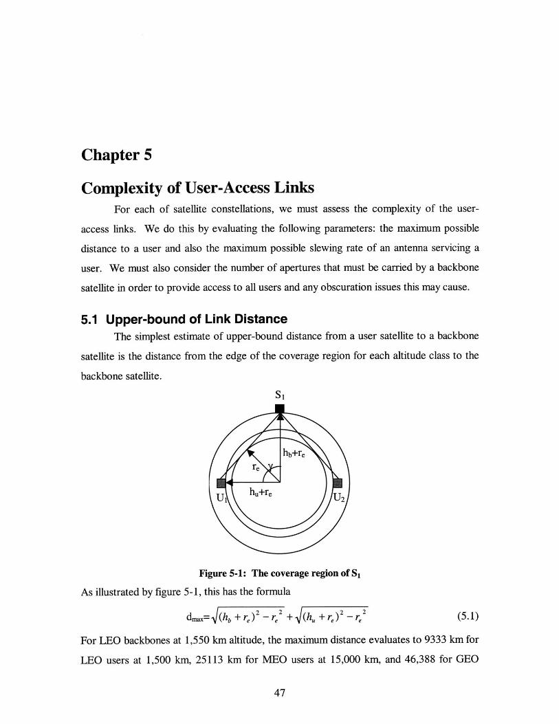
5.1 Upper-bound of Link DistanceThe simplest estimate of upper-bound distance from a user satellite to a backbone

satellite is the distance from the edge of the coverage region for each altitude class to the

backbone satellite.

SI

hb+re

re

U1 hu+re U2

Figure 5-1: The coverage region of S1

As illustrated by figure 5-1, this has the formula

dwa= (hb + r) 2 -r 2 + (h.+ r)2 r (5.1)

For LEO backbones at 1,550 km altitude, the maximum distance evaluates to 9333 km for

LEO users at 1,500 km, 25113 km for MIEO users at 15,000 km, and 46,388 for GEO

47

users. For MEO backbones at 15,000 km altitude, the result is 25,029km for LEO users,

40809 km for MEO users, and 62083 km for GEO users. For GEO backbones, the result

is 46,303 km for LEO, 62,083 km for MEO, and 83,358 km for GEO. These results are

summarized in table 5-1.

User LEO MEO GEOBackbone (1500 km) (15,000 km) (35,786 km)LEO (1550 km) 9333 km 25,113 km 46,388 kmMEO (15,000 km) 25,029 km 40,809 km 62,083 kmGEO (35,786 km) 46,303 km 62,083 km 83,358 km

Table 5-1: Summary of maximum distance from backbone to edge of coverage region

We do have an interest in reducing these maximum possible distance in cases

where it is possible and convenient, however, since maximum link distance is a greater-

than-linear factor in the cost of a cross-link, as we will later see. So, we will now look for

ways of reducing the maximum possible user-access link distance where possible.

For the GEO backbone, this can be easily done, since the GEO coverage region is

has radius >900 on user altitude classes. Thus, we can roughly divided each user altitude

region into thirds centered around the nearest GEO backbone satellite, with a generous

overlap of say 300 in order to accommodate make-before-break handoffs for LEO and

MEO users. This scheme essentially assign to each GEO backbone satellite the users

which are in the "half' of the user sphere closest to it, i.e. the users which are close to the

backbone satellite than to its antipodal position. The furthest LEO and MEO users, then,

would be on the edge of a coverage region of radius 900, meaning their distance from the

backbone satellite would be the hypotenuse of a triangle with sides re + hGEo and re +

hMEO/LEO. The furthest such users for MEO is then

(6,378+ 35,786)2 + (6,378 + 15,000)2 = 47,273 km away, and the furthest LEO users is

V(6,378 + 35,786)2 + (6,378 +1,550)2 = 42,902 km away. For GEO users, we would not need the

overlap for hand-offs, since the backbone satellite and the user remain stationary to each

other. Thus, we simply break up the GEO user plane into thirds centered around each

backbone satellite. This means that the furthest users will be at most 600 away from the

48

GEO backbone in central angle. If a user is 60' away on the GEO plane, the backbone

satellite, user satellite, and the center of the earth make an equilateral triangle, making the

maximum service distance re + hGEO = 6,378 + 35,786 = 42,164 km.

For the MEO and LEO backbone constellation, we will discover in the next

sections that in the interest of reducing aperture count, we utilize nearly the entire

coverage region of a backbone satellite, especially on the GEO user plane. Thus, the

distance from a backbone satellite to the edge of a coverage region remains a good

estimate for the maximum user-access link distance for MEO and LEO backbones. We

will summarize the revised estimates for maximum user-access link distance in the table

below.

User LEO MEO GEOBackbone (1500 km) (15,000 km) (35,786 km)LEO (1550 km) 9333 km 25,113 km 46,388 kmMEO (15,000 km) 25,029 km 40,809 km 62,083 kmGEO (35,786 km) 42,902 km 47,273 km 42,164 km

Table 5-2: Summary of estimated maximum distance of user-access link

5.2 Upper-bound of Slewing RateWe now wish to find the upper bound on the possible slewing rates of the user

link. For given backbone and user altitudes, we now argue that the maximum slewing rate

occurs when the user satellite and backbone satellite are right above and below one

another, meaning they are collinear with the earth's center. This is because this situation

minimizes the distance between the satellites, while the magnitude of the velocity vectors

of the satellites only depend on their altitudes and therefore are constant over all satellite

locations at given altitudes. We know that the rate of angle variation between the two

satellites is inversely related to the distance between them. Thus, if the magnitudes of the

velocity vectors are the same and we've minimized the distance between them, then we

have maximized the slewing rate between them. Thus, we achieve maximum slewing rates

when the two satellites are right above and below one another.

With this constraint, we can still rotate the velocity vectors with respect to each

other in order to find the maximum slewing rate for a single direction. This direction

49

occurs when the velocity vectors are at 1800 from each other, since in this direction the

magnitudes of the vectors contribute only to one direction. The physical situation that this

represents is two satellites orbiting in retrograde directions in the same orbital plane.

We now want to find an expression for the variation of the angle formed by the

link between two retrograde-orbiting satellites and the plane tangent to the orbit of the

backbone satellite over one period.

S 02

r 2

Figure 5-2: Calculating the maximum slewing rate in a retrograde satellite configuration.

Looking at figure 5-2, consider the link between S, and S2, with S1, the backbone satellite,

orbiting clockwise and S2, the user, orbiting counter-clockwise. If we were to stay in a

frame where S, remained stationary at the origin, we could consider S2 as rotating twice as

fast around the center of the concentric circles. Consider the angle that the link makes

with the y-axis when S2 has gone through a rotation of 0 degrees. We know that S2 has

the coordinates (r2cos(0)+ri, r2sin(0)). Thus, the angle p between the link and the x-axis is

tnrr 2 sin(O)tan-r 2 csi(O) , and the angle c, which represents the angle of "elevation" betweenr2 cos(O) +r,

the tangent of the backbone satellite and the link to the user satellite, is 90'-p.

Differentiating p with respect to 0, we obtain the expression j- _ r22 + rr2 cos

+r2 +2rr2 cosO

We know that 0 = 2$, where $ is the actual phase angle of the orbit, since we made an

50

adjustment in the frame of reference. Thus, we know that the slewing rate with respect to

phase angle is

dp= 2 = 2 r 2 +2r 2 cos(5.2)do dO 2 2

r, +r + 2rr2 cosODifferentiating and setting this expression equal to zero, we can see that it has extremal

values at 0 = 7r, which would make the maximum value of dp/dO equal to

22r2 -2rr 22 2 . (5.3)

r, +r 2 -2rr 2

Now we must find the relationships between $ and time in order to derive the

extreme values dp/dt. To do this, we must first find the time it takes for the satellites of

each altitude to complete a 3600 orbit. We do this using the following equation for

elliptical gravitational motion:

2 42(r, +rPGM (5.4)

where p is the orbital period, (r, + re) is the semi-major axis of the orbit (equal to the

radius for our case), G is the gravitational constant, and M is the mass of the earth. For G

= 6.672x10-' cm 3/g/s 2 and M = 5.974x1027 g, the orbital periods work out to 7026s for the

LEO orbit with an altitude of 1550km, 31,112s for the MEO orbit of 15,000km altitude,

and 86,400s for a GEO orbit. Since each of these times represent a 360' progression of $,

we can relate $ to t and thus d$ to dt for each of the orbits. Specifically, d$ = .0512/sedt

for the LEO orbit with h = 1,550 km, d$ = .0116'/sedt for the MEO orbit with h = 15,000

kin, and d$ = .0042/sedt for the GEO orbit with h = 35,786 km. Thus, the expression for

the maximum slewing rate is

2dp 2r 2 - 2rr2 * 360 (5.5)

= 2+22(.5dtn , +r2 - 2r, r2 42r r)

GM

For the LEO case where r1 =1,550 + re and r2 = 1,500 + re, this expression

evaluates to

-16.13 /s. As a sanity check, this is consistent with the result obtained by the method

illustrated in figure 29, which involves adding the two opposing instantaneous satellite

51

velocity vectors and then evaluating the angle of change at a distance d km away. The

expression obtained using this method is dpdt

v+v22tan {1 2

2d J , which evaluates to -

16.170/s.

d

v2 vI

Figure 5-3: A sanity check on slew rate calculations

We have plotted the max slew rate versus user altitude for the LEO and MEO

backbone cases below.

0

-2

-4

-6

[ -8-1

-10

-)Co)

x-12

-14

-16

-18

Max User Slew Rate for LEO backbone at 1,550 km

0 500 1000 1500User Altitude (kin)

Figure 5-4: Maximum slew rate of user-link for a LEO at 1,550 km altitude

52

0

-1

-2

-3

-4

-5

-6

-7

5000User Altitude (km)

10000

Figure 5-5: Maximum slew rate of user-link for MEO backbone at 15,000 km

At backbone altitude 1,550 km and user altitude 1,500 km, the plot of the slew rate versus

0 is as follows:

50 100 150 200 250Phase angle of user satellite

Figure 5-6: Slewing rate vs. Phase angle of usersatellite of 1,500km altitude with LEO backbone at1,550 km altitude.

53

Max slew rate for MEO backbone at 15,000 km

CaU1)

Cu,2

-8

-9

-100 15000

F-

0.4

0.2

o 0

0.2

-0.4

o -0.60I)

-0.8

-1

300 350

I I I

I l'

r -

as we can see, the slewing rate is a constant less than .1 /s for a majority of the orbit and

only increase to a maximum around -16'/s for a small band around 0 = 180' which

exceeds -10/s only for a band of less than 3 degrees from 0 = 178.50 to 181.5', as shown

in figure 5-7, a zoomed in version of figure 5-6.

0

-0.2

-0.4

-0.6

v -0.8

1.2

-1.4

-1.6

-1.8

178.5 179 179.5 180 180.5 181 181.5Phase angle of user satellite

Figure 5-7: A close-up of figure 5-6.

In the MEO case with a separation of 50 km between the two satellites, the region

of the user orbit where the slewing rate exceeds -1 /s is even narrower, ranging only from

0 = 179.50 to 180.50, as can be seen in the next figure.

54

0

-0.2

-0.4

-0.6

-0.8

-1

17 '7

Figure 5-8: Slewing rate vs. Phase

179 180 181 182Phase angle of user satellite

angle of user satellite with MEOaltitude.

183

backbone at 1550 km

For user altitude equal to backbone altitude, we have a situation where p is always

increasing at the rate as 0, by a geometric theorem. Thus, except for the instantaneous

change in direction at 0 = 1800, the slewing rate remains constant and is equal to dp/dt, or

the rate of change in phase angle with respect to time. This is .0512 O/s for the LEO case

and .01160/s for the MEO case.

Based on the very small proportion of user orbits around the backbone satellite

where the slewing rate exceeds the feasible range, we can conclude that service outage

due to tracking difficulty caused by excessive slewing rate can be easily overcome by

hand-off to a neighboring backbone satellite. And since these excessive slewing rates only

occur when a user satellite is near one backbone satellite, we can guarantee its visibility by

another backbone satellite, because backbone satellites were designed visible to at least

their neighbors in the same orbital plane in order to maintain intra-backbone links. Thus,

we can conclude that maximum slow rates do not pose a limiting consideration in the

choice of our constellation.

55

5.3 Number of Apertures Required for User SupportGiven the nature of high-rate space communication, antenna apertures must be

devoted to user connection on a one-to-one basis. Theoretically, the minimum number of

apertures that must be carried by the backbone constellation is equal to the expected

number of users. Additionally, it would be desirable for manufacturing reasons to place an

equal number these apertures on all the satellites forming the backbone. Thus, the most

ideal situation would be if each backbone satellite carried - apertures, where u is then

total number of users and n is the total number of backbone satellites.

In practice, however, more apertures will be placed on each backbone satellite than

the ideal theoretical minimum for several reasons. First, the geometry of backbone

satellite coverage affects how many apertures each individual satellite must carry. In the

first subsection, we will examine how the geometry of overlapping coverage regions

dictate the number of apertures carried by an individual satellite and determine an

expression for the number of apertures that a satellite must carry as a function of its

coverage characteristics. Next, we will look at the backbone-user combinations case-by-

case, beginning with the GEO backbone-GEO user situation, to see how many apertures

are necessary to provide service for each combination. To simplify analysis for this

section, we will assume that users of all orbital classes are uniformly distributed within

their space.

The second cause for an increased number of apertures onboard a backbone

satellite is the necessity of user hand-offs between backbone satellites. More than one

aperture must be devoted to a single connection in order to ensure a safe make-before-

break hand-off. Thus, at all times we wish to have some number of apertures free on each

backbone satellite in order to service these hand-offs, creating the need for satellites to

carry extra apertures over the number determined by geometry. We will examine the

hand-off requirements for each backbone constellation to see how they necessitate

additional apertures on each backbone satellite. As a conclusion, we will provide a

recommendation for the number of apertures that must be placed aboard the individual

56

satellites of each backbone constellation and also suggest physical locations onboard the

satellites for their placement.

5.3.1 Effects of Geometry on Number of AperturesConsider the coverage region of a single backbone satellite at a snapshot in time,

say sat 1 in figure 5-9. This particular backbone satellite is responsible for providing

service to all of the user satellites in its coverage region unless its region overlaps the

region of another backbone satellite, like the intersection between sat 1 and sat 2 in figure

5-9, in which case the users in the overlapping region can be divided among the two

backbone satellites. If there more than two overlapping regions (like the center region of

figure 5-9), then the users can be divided among all of the satellites with overlapping

coverage regions. Thus, a backbone satellites must provide one aperture for every

satellite in its single coverage region, one aperture for every two satellites in a coverage

region it shares with another backbone satellite, and so on. We capture this in the

equation

a = 1(5.6)

where aj is the number of apertures that backbone satellite j must carry, c is j's coverage

region, i is the level of coverage that the user experiences, and ui is the number which

experience i-levels of coverage.

Sat c Sat 21 2

2 3 2

Sat 31

Figure 5-9: The overlapping coverage regions of three backbone satellites.

57

Now given the uniform distribution of users assumption, we can modify the

previous equation as follows

aj = - dV (5.7)

where a, is the number of apertures that backbone satellite j must carry, cj is j's coverage

region, i is the level of coverage experienced by dV, u is the total number of users, and v

is the total volume of the space of possible user locations. We will assume that aj will be

the same for all backbone satellites, since orbital regularities will cause each satellite to

experience the same maximum level of user demand given the uniform user assumption.

In the most desirable case, we want this number to be - , where n is the number ofn

backbone satellites, for all satellites, which will waste the least number of apertures while

providing access for all users. We will now examine the backbone-user combinations

case-by-case to see if they will yield this desirable result.

58

5.3.2 GEO Backbone

5.3.2.1 GEO backbone-GEO User

When a GEO backbone is serving GEO users, each GEO covers 4 * co ReRe+h

= 325.2' of the GEO orbit, out of a total of 3600, as figure 5-10 illustrates. The coverage

gap of one single satellite is thus 360'-325.2' = 34.8'.

Si

4 9 COS RRe+ h)

Figure 5-10: GEO backbone coverage of GEO users.

For n > 2 evenly spaced backbone satellites and assuming a uniform distribution of

users, we theorize that the user load can be evenly split among the backbone satellites,

because the obscured region of each individual backbone satellite is small, thus facilitating

an easy division of users. For the common three-satellite GEO backbone, we see that this

is indeed that case. Referring to figure 5-11, we see that the coverage region of a single

backbone satellite includes 2*34.8* of double coverage and 6*42.60 of triple coverage.

Substituting this into equation 5.7, we get

2 6u( * 34.8 +-e 42.6'

23 Ia= r 3 (5.8)

3600

a . -3u

59

Thus, for ug GEO user satellites and 3 backbone satellites, the total number of apertures

Uthat each GEO backbone has to carry in order to service GEO users is -- }

3

Si

42.60 42.60

34.80 34.80

42.60 42.60

S3 42.60 42.6* S2

34.80

Figure 5-11: Illustration of the coverage regions of a 3-satellite GEO backbone

5.3.2.2 GEO backbone-MEO/LEO UserA GEO backbone satellite services MEO/LEO users from a "higher" altitude, that

is, from an orbit of greater radius than the user. As figure 5-12 suggests and equation 3.1

confirms, if we consider spheres of successively increasing radii in the LEO/MEO user

altitude ranges, the percentage of the sphere that can be covered by a single GEO satellite

monotonically increases with the radii. If coverage can be evenly divided amongst the

backbone satellites on all spheres of infinitesimal "thickness" and increasing radii within

the LEO and MEO altitudes, then we can naturally conclude that all LEO and MEO users

can be divided evenly amongst the backbone satellites, since we may simply "integrate"

the regions assigned to individual backbone satellite over all altitudes to produce an even

division of the total LEO/MEO user space. We need only to show that coverage of the

sphere at the lowest LEO altitude can be evenly distributed amongst GEO backbone

satellites in order to demonstrate the existence of an even distribution of coverage for the

whole LEO/MEO user space. This is due to the fact that coverage regions of individual

backbone satellites monotonically increase in size with increasing user altitude around the

60

same sub-satellite point. Thus, a valid distribution scheme of a low user altitude remains

valid at a higher user altitude, since the coverage region of a backbone satellite on a user

sphere of higher altitude is a superset of the coverage region of the same backbone on a

user sphere of a lower altitude. Thus, we will now demonstrate the existence of evenly

distributed coverage for a three-GEO constellation on a user sphere of 250km altitude and

conclude the existence of evenly distributed coverage for the three-GEO constellation for

all LEO and MEO users.

GEO Orbit Plane

S,Earthowl

MEO users

ED LEO users

Figure 5-12: A GEO backbone satellite providing service to the MEO and LEO user regions.

GEO Orbit Plane

M gap radius(@1500 km)= 62.80

Max gap radius(@250 km) = 81.40

Figure 5-13: The coverage gap for a GEO backbone and the LEO user region.

For a given user altitude, we recall that we can calculate the radius of coverage by

a single GEO satellite on the sphere at that altitude via the equation

y=cos- +cos-1 re (3.1)RI R2

where y is the radius in angular distance, re is the radius of the earth, R1 is the radius of the

backbone and R2 is the radius of the user sphere. For a GEO backbone and LEO users,

61

this coverage radius is smallest at the lowest user altitude of 250 km, with a value of

97.10, making the radius of the coverage gap 82.90. When the 250 km altitude user

sphere is projected onto a plane, this coverage profile will appear like figure 5-14, with

regions of single, double, and triple coverage.

3

B

1 2 c 1 a 2 1 2 1

A b C

Figure 5-14: The projection of a GEO backbone's coverage region on the 250 km altitudeLEO user sphere. The circles indicate the coverage gaps of individual backbone satellites,thus the numbers within the regions indicate the level of coverage of that particular region.

We will now use several equations from spherical geometry to calculate the

surface areas of the various regions, to determine if the GEO backbone can provide

maximally efficient service on this sphere. First, we calculate the area of each individual

circle, which is given by the formula

A = 2nR 2(1-cos r) (5.9)

Where R is the radius of the sphere and r is the radius of circle in central angle degrees.

For the GEO backbone and 250 km LEO user case, this area becomes 27CR 2(1-cos 81.9,)

= 5.51R 2 . Next, we must calculate the areas of the "overlap" regions between the circles,

which are the areas of single coverage with the help of three more formulas from spherical

geometry. The first is the law of sines for spherical triangles, which is

sinA =sinB sin (5.10)sin a sin b sin c

where A, B, and C are the angles of the spherical triangle, which are the angles formed by

tangents to the arcs representing the sides at their particular intersection, and a, b, and c

62

are the lengths of the sides of the spherical triangle measured in degrees of central angle.

The second is a formula for spherical right triangles, which says, for a spherical triangle

with a right angle at C,

cos A= sin B cos a . (5.11)

And the third is Girard's formula, which says that the surface area of a spherical triangle

with angles A, B, and C measured in radians is

At = R2(A+B+C-n) (5.12)

In order to find the area of the single coverage region, we will find the area of the "pie"

shaped region formed by A, B and B', subtract out the area of the triangle ABB', and

finally double this difference.

We first notice that ZC=90* because all of the subsatellite points are equatorial

and the coverage regions have equal radius. Next, we can label side b = 60', half of the

distance between subsatellite points, and side c = 82.90, the radius of the coverage hole.

We can then find ZB by the spherical sine formula

ZB = sin 90sin 60 =60.770. (5.13)

With this, we can find ZA by equation (5.11),

ZA = sin 1 cos 60.77 =77.590 (5.14)cos 60'

So, the area of the spherical right triangle ABC is

AABc= irR2 77.60+60.8 +900-1800 =.844R2, (5.15)1800

meaning that the area of ABB' is 1.688R 2. The area of the pie-shaped region is

APie = 2*77.69 *5.51R 2 = 2.375R 2. (5.16)360

So the area of one single coverage region is

Asingie= 2(2.375R 2 -1.688R 2) = 1.374R 2 (5.17)

The area of each individual double coverage region is

63

ADouble = 5.51R 2 - 2*1.374R2 = 2.762R2 , (5.18)

and the area of the triple coverage region is

ATriple = 41ER 2 -3(Asingle)-3(ADouble) = .157R 2 . (5.19)

Each individual satellite can see one single coverage region, two double coverage

regions, and all of the triple coverage region. Therefore, it is responsible for the following

fraction of users

1.374+ 2(2.762) .157

FGEO-LEO 2 333, (5.20)47r

which demonstrates that a three-satellite GEO backbone is capable of providing maximally

efficient coverage in terms of apertures to the 250 km LEO user sphere and thus to all

LEO and MEO users.

5.3.2.3 Hand-offsThe previous section took into account the distribution of apertures on the three-

satellite GEO backbone given uniformly distributed stationary users. We know, however,

that users do not remain stationary but travel in their orbit. Thus, we must take into

account the need for make-before-break hand-offs as users travel from the coverage

regions of one backbone satellite to another. Ideally, we can devote just one single

aperture to this task above and beyond the number required to provide normal service to

the users. To examine the feasibility of achieving this ideal situation, we will now estimate

the rate of hand-offs required to see if a single free aperture can keep up. We need only to

consider LEO users in this discussion. This is because GEO users are stationary with

respect to backbone satellites, and the large (radius ~90') overlapping coverage regions

and long user orbital periods at MEO altitudes provide periods of hours in which a hand-

off can be performed, making scheduling a simple task. Thus, we will only consider the

LEO users..

A hand-off is only truly necessary when a satellite travels from one single-coverage

region to another single-coverage region. Thus, in our calculations, we will adapt the

estimate that half of the user within a single-coverage region will travel toward the

eastwardly neighboring single-coverage region and half will travel toward the westwardly

neighboring single-coverage region. We also consider all of these satellites to be at a

64

uniform altitude and the path they must travel between single-coverage regions to all have

the shortest distance, which is the distance along the equatorial orbit. Referring to figure

39, this distance is twice the difference of the distance between sub-satellite points and the

radius of the coverage hole, which for the 250km orbit is 2*(120-82.9o)=74.2'.

Estimating the orbital period to be 90 minutes, this leaves 74.2/360*90=18.5 minutes

perform all of the hand-offs. The single coverage region has a surface area of 1.374R2 ,

which is 1.374/(4n) = .11 of the total surface area of the sphere. Thus, we can expect a

maximum .11 of the total number of LEO users to require hand-off to a particular satellite

at a time. With 30-40 LEO users expected in total, this means that at most 4-5 satellites

will require transition to a particular backbone satellite at a time. With 18.5 minute as the

shortest amount of orbit time between single coverage regions, this allows an average of

at least 3 minutes per hand-off, which should be a rate that can be maintained even

considering antenna slewing time and also time required to negotiate a new connection.

Thus, for a 3 satellite GEO backbone, one additional aperture per satellite seems sufficient

to meet the necessary hand-off requirements.

5.3.3 MEO Backbone

5.3.3.1 MEO Backbone-GEO UserTo begin our analysis of the MEO backbone, we must first consider if it can

effectively provide coverage for GEO users. This analysis differs from that of a GEO

backbone serving GEO users because the MEO backbone satellites orbit in planes

perpendicular to the GEO user plane, whereas GEO backbone satellites remain co-planar

with GEO user satellites. Thus, the amount of coverage that a constellation of MEO

satellites can provide to the GEO user plane varies dynamically over time. In our analysis

of MEO backbone with GEO users, then, we will develop a simplified dynamic model of

the visibility of the GEO user plane to the MEO backbone satellites and use this simplified

model to determine the efficiency of MEO backbone coverage for GEO users.

The profile of the coverage region of a single MEO satellite is shown in figure 5-

15 below. As one can visualize, while the MEO backbone satellite S1 is above the

equator, its view of the opposite side of the GEO orbit plane is obscured by the earth.

65

This obscuration begins to lessen as Si orbits toward the polar regions until all of the GEO

orbital plane is visible when Si nears the polar regions. From figure 40, the place at which

this total visibility occurs is at

1800- cos-1 re - cos-1 re =26.1* (5.21)r + 35,786 r, + 15,000

past the equator.

0E Polar Orbit

S1

1-5,-0 km ah

E GEO Orbit P ne re35,786 km

Figure 5-15: The visibility of the GEO orbit plane from a MEO polar orbit.

By examining the tangent line at that location, however, we realize that in order to

utilize this "visibility" by providing service to the entire GEO, a MEO satellite at this

altitude would have to mount apertures on both its "earth-facing" surface and the surface

opposite that one, which we call the "space-facing" surface. We would like to avoid

apertures on the space-facing surface, since they do not point toward any possible users

when the backbone satellite is near the poles. On the other hand, apertures mounted on

the earth-facing surface always point toward possible users of various altitudes. Thus, we

would like to find the point where the whole GEO plane is visible from the earth-facing

surface. This occurs when the tangent to the MEO polar orbit intersects the GEO orbit

ring, which is illustrated in figure 5-16. Si is at

Cos-1 re+15,000 = 59.50 (5.22)re +35,786

66

past the equatorial plane when this occurs. Thus, we can say that for 600 portions

centered around the poles, the MEO backbone satellite can service all of the GEO plane.

Now, for the rest of the orbit, we make the simplifying assumption that the

obscuration due to the earth is the same as it is when the backbone satellite is at the

equator. Since the earth's circumference is greatest in the equatorial plane, we can

assume that the obscuration of visibility from the polar MEO satellite orbit to the

equatorial GEO orbit is greatest over the equator. Our assumption is then a worst-case

simplification, whereby if there is any obscuration, we assume it to be have the greatest

effect possible.

S, MEO Polar Orbit

15,000 km

GEO Orbit lane E h

35,786

Figure 5-16: Full visibility of the GEO plane from a polar MEO using only the earth-facingsurface.

When the MEO backbone satellite is over the equator, its visibility of the GEO

orbit is shown in figure 5-17. The equation for the "hole" in visibility is

67

Si 15,00 k 35,786 km

MEO Polar Orbit Plane

GEO Orbit

Figure 5-17: The visibility of the GEO plane from a MEO satellite 15,000 km over theequator.

2*(180'- cos- re .- cos-1 r ) = 52.20 (5.23)r + 35,786 r + 15,000

Thus the MEO backbone satellite above the equator is visible to 308' of the GEO orbit.

If we wanted only to utilize the earth-facing plane of the backbone satellite,

however, the region of visibility is reduced. We must subtract out cos- 1 re + 15,000 _re + 35,786

59.5 from each semi-circle of the GEO orbit, meaning that the visibility is now reduced to

two 94.5' portions of the GEO plane which are reflections across the plane of the polar

MEO orbit. We will consider these two regions to constitute the coverage provided any

satellites experiencing obscuration.

We now consider the service provided by the MEO constellation on the GEO orbit

plane. If we consider a single polar orbit with 4 evenly spaced MEO backbone satellites,

the satellites are separated from each other by 90'. This implies that in the worst case, all

four satellites in a MEO backbone satellite plane will experience some obscuration. The

68

first two of these satellites experience obscuration on one side of earth and the other two

satellites on the other side of the earth. Thus, we consider the two sets to both be at the

equatorial latitude but directly opposite each other. We model their coverage regions as

that bound by the thin solid lines and the thin dotted lines in figure 5-18, with two

satellites per coverage region. The second orbital plane, which is perpendicular to the

first, adds two more sets of regions, those bound by the thick solid and thick dotted lines.

With a bit of calculation, we find each of the small overlap regions to be 4.4'. The top,

bottom, left, and right regions are 52.20, and the diagonal regions are 29.0', as illustrated

on figure 5-18. The 4.4* regions experience 6-fold coverage, while the 52.20 and 29.0'

regions experience 4-fold coverage. Thus, the fraction of users for which one backbone

satellite is responsible amounts to

4.40 29.00 52.203. + +

FMEO-GEO 6 4 4 (5.24)3600 8

Thus we can see that apertures servicing GEO users can be evenly divided amongst the

earth-facing surfaces of all of the MEO backbone satellites.

69

52.20

4.40 4.40

I I29.0*

GEO Orbit \

Figure 5-18: The coverage profile of the MEO constellation on the GEO user orbit.

5.3.3.2 MEO Backbone-MEOJLEO UserFrom equation 1, we have calculated the service radius of a MEO satellite at

15,000 km altitude on the LEO sphere at 250 km altitude to be 88.40. Because this is

nearly 90', we know that the coverage region of a single backbone satellite is nearly a

semi-sphere. Thus, if we consider the service provided by a single MEO plane, which has

4 satellites separated by 900 each, we can visualize that the only holes in coverage are

extremely small opposing areas on the user plane's equator 900 away from the intersection

of the equator with the orbital tract. We will thus proceed with the analysis of the

coverage profile of a single MEO plane to show that the hole in single-planed coverage is

insignificant and then make remarks about the optimality of double-planed coverage.

In figure 5-19, we've borrowed the diagram from the GEO case and modified it to

suit the need of the MIEO case. We must now view the long side of the rectangle as an

70

entire unrolled polar orbit path and the short side as only one-half of the equator. Also,

the circles now indicate coverage regions rather than coverage holes, and the integers

indicating the level of service enjoyed by each region has been modified accordingly.

However, the spherical geometric identities used to calculate the areas of the service

regions still apply, and we use them again here.

B'

2 1 C 2 a 1 2 1 2 1 2

A br- C

S

B'

Figure 5-19: A rectangular projection of the coverage profile of one plane of the MEObackbone on the 250 km LEO sphere.

We first find the area of each spherical circle to be 6.11R 2 using equation 5-9. We also

know that side c is equal to 88.40 from the coverage equation and that side b is equal to

450, one-half of the separation between the satellites. We also know that angle C is 900

because a segment joining the intersections of two circles and a segment joining their

centers must be perpendicular. With the spherical law of sines (5-10), we find that angle

B is 45.02'. We then find angle A to be 88.39' using equation 5-11. This then tells us the

area of the pie-slice BAB' is

Apie = 2(88.39) 6.11R 2 = 3.00R2 . (5.25)360

The triangle BAB' has area 2iTR 2(88.39+45.02+90-180)/180, which is 1.515R 2. This

means that the double coverage section has area

Aouble = 2R 2(3.00-1.515) = 2.97R 2 (5.26)

and that the single coverage section has area

Asingie = 6.11R 2-2(2.97R 2) = 0.17R2 . (5.27)

71

We can use these two values to compute the area covered by a single MEO plane, which

is

Apane = 4 (Asingle)+ 4 (Aouble) =12.56R2 . (5.28)

The entire area of the sphere is 4tR2 , which is about 12.5664R2 , meaning that a single

MEO orbit can cover approximately 99.95% of the 250 km altitude LEO user sphere, with

the miniscule holes in coverage occurring around 90' from the sub-satellite points, or

exactly on the path traced out by the sub-satellite points of the second plane, meaning that

they are certain to be covered. Since it provided by just a single plane, this coverage is

also not subject to variation in time, thus we do not have to worry about "worst-case"

situations occurring for an individual satellite.

Let us now consider the fraction of the users for which a single satellite would be

responsible given only one backbone plane. We know that it provides single coverage for

an area of Asingie = .17R 2 and shares coverage with another satellite over 2 Adoubie =

2(2.97R 2). This means that the fraction of users it is responsible for is

.17+ 2(2.97)

4r 2 - .2499, (5.29)

which is nearly of all of the users, with the slight difference resulting from the coverage

gaps. We can safely estimate that outside the minute gaps, a single MEO plane can

provide maximally efficient coverage of the portion of the 250km LEO sphere to which it

is visible. With two planes, the MEO constellation easily covers the any gaps, and we also

know that covering the small gaps will hardly contribute a significant portion of users to

any one plane's load. Thus, we can conclude that with two planes, a MEO backbone

constellation can provide maximally efficient coverage of the 250km LEO sphere and, as

we previously argued, the entire space of LEO and MEO users.

5.3.3.3 Apertures for Handoffs

Regarding handoffs, we know that >99.5% of the space of all users will experience

coverage by at least 2 backbone satellites at all times, if not by more, simply due to the

overlapping coverage areas of the planes. We also know that the contiguous coverage

region that a MEO satellite provides is at least the size of the GEO plane and also at

least the size of the LEO/MEG user spheres. Multiple levels of coverage over large

72

contiguous coverage regions allow a large amount of time for each handoff, on the order

of up to half a user orbital period. Thus, we can safely conclude that each backbone

satellite need only carry 1 more aperture in order to accomplish make-before-break

handoffs. Our MEO backbone constellation is thus completely optimal in terms of

aperture assignment, just as our GEO backbone constellation was.

5.3.4 LEO Backbone

5.3.4.1 LEO Backbone-GEO UserWe now analyze the coverage that a single LEO backbone provides to the GEO

orbit ring, in much the same manner as our MEO analysis was conducted. For a polar

plane of LEO backbone satellites, full visibility of the GEO orbit plane occurs at

LEO Polar Orbit

Si

h

GEO Orbit Plane 35,786 km

Figure 5-20: The visibility of the GEO orbit plane from a LEO polar orbit.

1800-cos-' re 6 -cos _1 r J = 62.30 (5.30)re + 35,786 re + 1550

past the equatorial plane. In order for us to utilize only the bottom surface for apertures,

however, full visibility occurs at cos, re+1550 )= 79.20 past the equatorial plane,re +35,786

meaning that only for two 20' window near the poles will the LEO satellites be able to

service all of the GEO backbone. Since 450 separate each satellite in a 8-satellite LEO

plane, in the worst case, all of the LEO satellites in one plane will undergo obscuration by

the earth.

When a LEO backbone satellite is at the equator, it experiences the maximum

obscuration by the earth, which renders

73

2*(180'-cos-! re -Cos_1 re ) = 124.60 (5.31)re + 35,786 ) re + 1550

of the GEO orbit invisible to it. Thus, at least 235.40 of the GEO orbit are visible to a

LEO satellite at all times.

If we wanted to use only the bottom surface of the LEO satellite for service,

however, then we must subtract out cos~1 re+1550 = 79.2' from each half of the servicere+35,786

region, leaving two regions of 38.5' as the region serviced by each LEO satellite. Figure

5-21 illustrates the basis for these calculations. Thus, we will model the coverage region

of every LEO backbone satellite experiencing obscuration to be two 38.5' regions which

are reflections across the orbital plane and are separated from each other by 124.6'.

These regions are illustrated to scale in figure 5-22 as the regions bound by the boldest

lines with angle measurements between them.

35,786 kmn

S, Sire

GEO Orbit

LEO Polar Orbit Plane

Figure 5-21: Service region provided on the GEO user orbit bya LEO backbone satellite using only its earth-facing surface.

74

Now, we can freely assign a backbone satellite to cover only the users within a

certain sub-region of its region of visibility. For reasons which will soon be apparent, we

will require that a backbone satellite only cover the regions of the GEO plane between the

thinner lines, i.e. two 180 regions sharing a diameter as one border and with their other

borders separated by 144'.

The 8 satellites in the same orbital plane can be split in half, with 4 satellites on one

side of the earth and 4 on the other side. Thus, the coverage region of an entire plane is as

shown in bold in figure 5-23, with two opposing 360 regions sharing two lines as their

boundaries. When this region is replicated five times with a rotation of 72' between each

replication, we see that it exactly covers the 3600 GEO user circle with no overlapping

regions. In order to achieve this coverage, each satellite is responsible for 360 of the

plane, with each 360 region experiencing 4-fold coverage. Thus, each satellite is

responsible for

36

FLEO-GEO = = (5.32)360 40

of the users, demonstrating that the LEO backbone distribute the coverage of the GEO

user plane in a maximally efficient manner.

75

EO Orbit

Figure 5-22: The coverage region of a single LEO backbone satellite experiencingobscuration from the earth on the GEO user orbit. The actual limits of visibility are markedin bold, while the coverage region used to prove optimal aperture division is bound byregular lines.

36*

EO Orbit

Figure 5-23: A designed coverage profile of the LEO backbone constellation on the GEOuser orbit

76

180

38.5

124.60 1440

38.

180

5.3.4.2 LEO Backbone-MEO/LEO userWe must now consider the case of a LEO backbone servicing MEO and LEO

users. Here is another case where the user are distributed in spherical spaces and the

backbone satellites are in polar orbits, like the MEO backbone-MEO/LEO user case.

Thus, we must first examine the lowest user sphere, at 250 km altitude, to determine if

maximally efficient coverage is feasible. In the case of the LEO backbone, with 5 planes

of 8 satellites each, it is difficult to analytically compute the full coverage profile with all of

the intersections and regions. Instead, we shall use an engineering estimate to argue for

the infeasibility of maximally efficient coverage provided by the LEO backbone.

We know that in order to provide maximally efficient coverage, each backbone

satellite must be responsible for an equal and minimal amount of users at all times. For the

40-satellite LEO constellation, this means that each satellite can be responsible for no

more than 1 / 4 0 th of all of the users at one time. Assuming that each backbone satellite

services all of its "visibility region," which is great in size than 1 / 4 0 th of the entire 250km

LEO sphere, over its whole orbit, we know that there must be multiple levels of coverage

on these regions at all times in order for the backbone satellite to be able to "share

coverage" with follow backbone satellites and achieve this maximally efficient service.

Indeed, this is how the MEO backbone constellation, in which the visibility region of each

backbone satellite is nearly of the 250km user sphere, achieves maximally efficient

coverage. We will see that this cannot be the case for the LEO backbone, however. On

the 250 km altitude LEO user sphere, the 1550 km LEO backbone satellite has a service

region with radius 51.7*. This service region has area

2mR 2 (1-cos(51.70)) = 2.389R 2 . (5.33)

This is 2.389 = .19 of the whole sphere. Thus, if the entire visibility region of a LEO47r

backbone satellite were single coverage, a single backbone satellite would be responsible

for .19 of all the users, which is obviously not optimal. In order to achieve optimality, a

LEO backbone satellite must average a service level of 1 = 7.6 fold over its coverage40

region at all time over its orbit. This number, however, is unachievable, since a satellite

only has 6 nearest neighbors, as shown in figure 49. Thus, if all neighboring satellite's

77

coverage region covers So's sub-satellite point, we then have a region of seven-fold

coverage around the sub-satellite point of So. This is indeed the case for the LEO

backbone, since the distance between backbone satellites within the same plane is only

45 0 and the distance to the nearest satellites in the neighboring planes also does not

exceed 51.70, the coverage radius of one satellite. As an aside, this allows us to use only

one additional aperture per backbone satellite to achieve make-before-break handoff, since

it demonstrates the large regions of multiple coverage in the LEO coverage profile, thus

allowing for a long time period in which to schedule hand-offs.1

S2

S3

Figure 5-24: The six nearest neighbors of satellite So.

While seven-fold coverage exists for the LEO backbone constellation, averaging a

coverage level of 7.6 requires large regions where the coverage level is in excess of seven.

This extra coverage cannot come from satellites within the same plane, since their distance

to each other always remains fixed. The next nearest satellites other than the ones

pictured are two planes away with the same phase angle as So. While So is near the

equator, however, those satellites are 72' away from So, since there are a total of five

orbital planes. They are too far to cover So's sub-satellite point. Thus, in the worst-case

equatorial regions, So would not be able to a achieve 7.6-fold coverage and would thus be

responsible for providing service to more than 1/4 0 1h of the users at that time, thus

1 As an aside, this allows us to use only one additional aperture per backbone satellite toachieve make-before-break handoff, since it demonstrates the large regions of multiplecoverage in the LEO coverage profile, thus allowing for a long time period in which toschedule hand-offs.

78

requiring it to carry more apertures. Hence, we know that a LEO backbone constellation

cannot provide maximally efficient service to LEO/MEO users.

A LEO backbone satellite contains one additional deficiency in its provision of

user-access apertures. Figure 5-25 diagrams how a LEO would provide service to the

LEO/MEO sphere.

S, Earth

MEO users

LILEO users

Figure 5-25: The service area of a LEO backbone satellite on the MEO and LEO userspheres.

We can see that the LEO backbone satellite can provide service for all of the LEO users

by just using the earth-facing surface of the satellite. In order to provide service for all of

the MEO regions to which it is visible, however, the LEO backbone satellite must utilize

both the earth-facing surface and the "space-facing" surface. The lack of apertures on that

"space-facing" surface would remove a circle of radius cos- 1 re+1550 =4 5 .8' from there+5000)

service region of a LEO backbone on the lowest MEO user sphere. The service region

has a radius of cos' re + Cos- re = 92.3*, so this removal results in a loss of( re+1550) re+5000

about 30% of the service region, a significant portion. So, the LEO backbone satellite

must carry apertures on its "space-facing" side to avoid this loss. The location of these

apertures prevent them from being used to service for LEO users, whereas on MEO and

GEO backbone satellites all apertures can be used to service users of all three classes.

79

These apertures must be considered "extra" apertures used for filling in the gaps in the

MEO coverage region. The presence such apertures introduces an inefficiency into the

aperture assignments, since we must also provide apertures on the earth-facing service for

MEO users, because the majority of the MEO coverage area for a backbone satellite still

faces that side. While it may be theoretically possible for us to decrease the number of

apertures facing earth because some MEO users are served by apertures facing away from

earth, we still must provide earth-facing apertures in order to serve a majority of MEO

users. Because of the large number of LEO backbone satellites (40) and the relatively

small number of MEO users (-20-30), we can handle all MEO user conditions with one

space-facing and one earth-facing aperture on each backbone satellite. But this represents

80 apertures for only 20-30 users, and only the 40 earth-facing apertures can also be used

to service other user altitude classes. The service gap has caused us to introduce an large

number of excessive apertures into the entire satellite system. Thus, we can conclude that

the LEO constellation suffers a disadvantage in terms of the efficiency of aperture-to-user

assignment when compared to the MEO and GEO constellations.

80

Chapter 6

Cost Analysis

We have seen that both the MEO and GEO constellations can distribute apertures

for user support in a maximally efficient manner, while the LEO constellation suffers some

inefficiencies. However, despite their importance, apertures are only a part of the entire

satellite communications system. In order to gain a fuller understanding of how our

candidate constellations compare to one another, we must now estimate their whole

system cost using a speculative cost model. We will center this model around the

communications links of the system, certainly, but we also include such fixed costs as the

body of the satellite and the launch costs. We begin by introducing the cost equation of

our cross-links and proceed by dividing the costs of the entire system into our familiar

classifications of the cross-links.

6.1 Cost EquationThe cost of an optical cross-link has been previously modeled in [6] as a function

of distance and data rate to be

Coptica = ko + k, R 4d 2 (6.1)

where ko is the fixed cost of an optical link, k, is the coefficient associated with the

variable cost of a cross-link, R is the data rate required over the link, d is the distance of

the link, and a is an exponential factor between 2 and 3. Because of the high rate nature

of our communications, we will project every cross-link in our system to be optical and

thus use this equation to model the

cost of every link.

81

6.2 Cost Coefficients of Satellite LinksIn the cost analysis of a cross-link, we need to define the cost coefficients ko and

ki, which are applied to the fixed and variable costs of a cross-link respectively, and also

the exponent a. In [6], a was set to 3 and three sets of ko and ki were defined.

1. ko = 1.000x10 3 , k, = 5.654x10-9

2. ko = 5.000x105 , k, = 4.243x10~9

3. ko = 1.000x10 6 , k, = 2.828x10-9

all of which yield a cost of 2 million dollars for a link of 10Gbps with a range of 50,000

km. The first set represents a situation where the fixed cost contributes minimally to the

cost of the aperture, while third set represents a situation where fixed cost is predominant.

The second set is a medium between the other two. We will utilize these coefficients in

our cost analysis.

6.3 User-Access Links

6.3.1 Cost ParametersThe first type of communications links in our system is the user-access link, which

occurs between the user and a backbone satellite. If a satellite constellation can support

users optimally, the number of such links in the whole constellation is very close to the

number of projected users in the systems, plus one extra link per backbone satellite for

hand-offs. The exact equation for the number of links required given an optimal

distribution is

L= T - (6.2)T

where T is the number of backbone satellites in the system and u is the number of users in

the system. This equation applies for the GEO and MEO systems. Assuming 100 users in

the system, GEO requires 105 apertures and MEO requires 112.

For a non-optimal system like LEO, we must project the exact number of user-

access apertures required. We know that the LEO constellation requires apertures facing

away from the earth in order to fill in the service gap in the MEO region. As said in the

previous section, one such aperture is enough to handle this task. As calculated in the

82

pervious section, around 30% of the MEO users will be handled by these apertures. The

other 70% of MEO users must be serviced by the downward-facing apertures, which also

service the other user altitude classes. We must also remember the single aperture

required for hand-off. Thus, the number of links required for a LEO constellation is

LLEO 7m+(um) +2 (6.3)

where T and u are as before and m is the number of MEO users. For a total of 100 users

and with 25 MEO users, this yields 200 total apertures in the LEO system. For all of the

rest of our analysis, we will assume that MEO users make up 25% of all of the users. This

makes our equation

LLEO .925u +2 (6.4)

For each user, we must provide for the maximum possible requested rate, which

was projected to be 100Gbps. We must also provide this maximum rate at the maximum

projected link distance, which was determined for each constellation in a previous section.

Thus, for a given set of constant coefficients and exponents, the cost of each user-access

link is actually fixed. Thus, the total cost of all of the user-access links in the system is

actually only dependent upon the number of users in the system. Thus, we will consider

the contribution of user-access links to the cost of the constellation to be only a function

of the total number of users. We list the parameters which contribute to this cost for each

constellation in the table below.

Table 6-1: Cost Parameters of User-Access Links

83

6.3.2 Numerical Examples of User-Access Link CostWe can now plot some numerical examples of user-access link cost for each type

of constellation. Each of the following plots are the costs for all of the user-access links of

the entire constellation, not just for each satellite, as a function of the number of users.

The total cost of the user-access links in the system equals the total number of apertures in

the system times the cost of each individual link. The results are shown below.

X 109 Coefficient Set12.5

2

1.5

0

0.5 GEO.- MEO

3X= .- ' LEO

oT 1

-- GE

0 20 40 60 80 100Number of users, u

Figure 6-1: Cost comparison of system-wide user-access links for the first coefficient set (ko =1.000x103).

84

Coefficient Set2

40 60Number of users, u

Figure 6-2: Cost comparison of system-wide user-access links for the second(ko = 5.000x105).

x 1014 r

coefficient set

Coefficient Set3

12 -

10

60

o 4

2

0

I- GEOo MEO

-- LEO

)


Figure 6-3: Cost comparison of system-wide user-access links for the third coefficient set (ko= 1.000x10 6).

85

x 1018

16 -

14 -

12 -CU,

co

0

10

8

6

4 l

2

C0

0 20

- - GEOo MEO--- LEO

80 100

6.4 Intra-Backbone Links

6.4.1 Cost ParametersIntra-backbone links are the cross-links which occur between a pair of backbone

satellites. We will now proceed in much the same fashion as we did for user access links

to find the parameters which contribute to the cost of the constellation's backbone links.

First, we know that most polar satellite constellations are implemented with four

backbone cross-links per satellite, two being intra-plane and one to the nearest

neighboring planes east and west. This is what we will assume for the MVIEO and LEO

constellations. For the GEO constellations, however, we will assume the presence of only

two cross-links per satellite, since the GEO is only a planar constellation.

We have also already calculated the maximum distance of the cross-link for all

constellations in a previous section. Thus, the only significant parameter left to determine

is the data rate capacity required for each link. We will rely heavily on [6] for this

calculation and utilize the uniform traffic assumption introduced there. Under this

assumption, there is a total level of traffic T, in the entire system, and the same amount of

traffic originates from each backbone satellite. The traffic originating from one backbone

satellite is also sent equally to all backbone satellites, including itself. Thus, each

backbone-backbone pair (including duplicates) of source-and-sink contains an equal

amount of traffic. We will also model T, as a function of the total number of users in the

system, with a minimum of lOuGbps and a maximum of lOOuGbps.

With this assumption, we can enumerate nine such different pairs for the GEO

constellation. Assuming shortest-path routing, which makes each source-sink path either

one or zero hops, we easily find that each intra backbone cross-link is responsible for two

of the nine pairs. Thus, for GEO, we know that the maximum capacity required of each

cross-link is 2 T.9

With MEO and LEO, we utilize the seamed network modeled described in [6],

which tells us that the data-rate capacity required for both inter-plane and intra-plane

cross-links is " , where M is the number of planes in the backbone constellation. Thus,8M

86

TTfor MEO, the capacity required is - , and for LEO, the capacity required is -u-. The

16 40

table below summarizes the parameters which determine cost for the intra-backbone cross-

links in the system.

Constelation GEO MEO LEO

Total no. of apertures 3.2 = 6 8*4= 32 40.4=160

Maximum data rate of link 2 TU TUas a function of T 9" 16 40

Maximum intra-plane 73,030 km 30,233 km 6,068 kmlink distanceMaximum inter-plane N/A 32,371 km 5,715 kmlink distance

Table 6-2: Cost parameters of the intra-backbone link

6.4.2 Numerical Examples of Intra-Backbone Link CostsHaving established the equation for the cost of all the intra-backbone links of a

satellite constellation, we can now compare that cost for the LEO, MEO, and GEO

constellations under various circumstances. We will of course utilize the three sets of cost

coefficients to represent different contributions of fixed satellite cost as before, but we will

now also vary Tu to represent situations of low system traffic, medium system traffic, and

high system traffic. We will choose T. equals 5uGbps to represent low system traffic,

since this means that the average user demand is only 5Gbps, on the low end of our

projections. It then follows that 20uGbps represents the Tu for situations of medium

traffic demand and 1OOuGbps should represent situations of high traffic demand. These

cases affect the data-rate capacity that must be carried by each intra-backbone links. The

plots resulting from each situation were generated and are now presented below.

87

x 107 Coefficient Setl, Tu=5uGbps14 -

12 -

10 -

C8

0

60

0 GEOS4^ 0' MEO

-- LEO

2

0(0 20 40 60 80 100

Number of users, u

Figure 6-4: Cost comparison of system-wide backbone links for the first coefficient set (ko =

1.000x103) and low traffic conditions

7x 10 Coefficient Set2, Tu=5uGbps

10

9

8

7

06

4 -0 GEO

3 o MEO

2 -

1-

0.0 20 40 60 80 100

Number of users, u

Figure 6-5: Cost comparison of system-wide backbone links for the second coefficient set (ko= 5.000x10 5) and low traffic

88

7x 10 ' I I V U U - U U zJ

18 -

16

14 -

co,12 -

o 10 -

8.0

0

4 - G '

0 MEO2- LEO

00 20 40 60 80 100

Number of users, u

Figure 6-6: Cost comparison of system-wide backbone links for the third coefficient set (ko =1.000x10 6 ) and low traffic

x 103 Coefficient Set, Tu=20uG bps4

3.5 -

-3 G

C',

2.5

a)0.


Figure 6-7: Cost comparison of system-wide backbone links for the first coefficient set (ko=1.00ox103) and medium traffic

89

C, ffi i S 31 Tr rz Gb

x 10 Coefficient Set2, Tu=20uGbps3

2.5

2

0

0

.0

.1.5-

0

.0.

-- GEO0.5 0 MEO

-- LEO

00 20 40 60 80 100

Number of users, u

Figure 6-8: Cost comparison of system-wide backbone links for the second coefficient set (ko= 5.000x10 5) and medium traffic

8X 10 Coefficient Set3, Tu=20uG bps

2

~&1.4

S1.2 -1 -

-. - E

0.8 -

0.4 -

0.2 -

00 20 40 60 80 100

Number of users, u

Figure 6-9: Cost comparison of system-wide backbone links for the third coefficient set (ko =

1.000x106 ) and medium traffic

90

x 10 Coefficient Set1, Tu=lOOuG bps14 -

12

10

c80

- LE

0

CU0

2


Figure 6-10: Cost comparison of system-wide backbone links for the first coefficient set (ko =1.000x10 3) and high traffic

x 108 Coefficient Set2, Tu=lOOuGbps10

9

8

7

U 60

440 ' - GEO0 MEO

03 - LEO

2

0(0 20 40 60 80 100

Number of users, u

Figure 6-11: Cost comparison of system-wide backbone links for the second coefficient set (ko= 5.000x10 5 ) and high traffic

91

> 10 Coefficient Set3, Tu=lOOuGbps

6 -

-_lie

c40

. GE

0

0

0 MEO-- LEO


Figure 6-12: Cost comparison of system-wide backbone links for the third coefficient set (ko =

1.000x106 ) and high traffic

6.5 Cost Equation of Entire ConstellationThe cost equation of the entire constellation consists of the sums of costs of the

user-access links, the backbone-links, the fixed cost of the satellite body, and the launch

costs for all of the satellite in the constellation. Although ko is the coefficient of fixed cost

for the communications link, it can also be used as a sensible estimate for the fixed cost of

the satellite body, since it models the cost of supporting the apertures as increasing

proportionally with the number of cross-links. As an example, it reasonably models a

GEO backbone satellite carrying 30-some user access links and 2 intra-backbone links as

having around five times the fixed cost of a LEO backbone satellite with 4 user-access and

4 intra-backbone links. We do not, therefore, need to include a separate constant for the

cost of a satellite body.

As for satellite launch costs, NASA's Cost Estimating Group provides data on

expendable launch vehicles to orbits of various altitudes [7]. Using data from their web

page, we estimate the launch cost of each LEO satellite to be around $30 million, the

launch cost of each MEO satellite to be around $150 million, and the launch cost of each

92

GEO satellite to be around $400 million. Thus, the final equation for the cost of the entire

constellation is

Cconsteliation = Nuser-access inis*Cuseraccess lin + Nbackbone links* Cbackbone link + Caunch, (6.5)

where Nuser-access links is the number of user-access cross-links and Nbackbone links is the number

of backbone cross-links.

6.6 Numerical ExamplesWe now add the projected launch costs to our previous cost estimates for the two

types of links to produce a final estimate of system cost. There were again nine

permutations of three coefficient sets and three traffic conditions. The plots resulting from

each permutation are now presented below.

X 109 Coefficient Seti, TU = u*5Gbps

C

0

0

(0

3.5

3

2.5

1 .5

1 L-0

I- - GEOo MEO

- LEO

) --

20 40 60Number of users, u

80 100

Figure 6-13: Constellation cost comparison for smallest contribution of fixed cost (ko =

1.000x10 3) and low system traffic

93

GMD

ax=m

x 103 r

Coefficient Set2, TU = u*5Gbps

2.8 -

2.6

222.4

0S2

0

0 1.80

1 .6

1 .4

1 .2

Figure 6-14:

- - GEOo MEO

LEO


Constellation cost comparison for medium contribution of fixed cost (ko =5.000x105) and low system traffic

Coefficient Set3, TU = u*5GbpsX 10

2.6 -

2.4 -

2.2 I

- - GEOo MEO

- LEO

0 20 40 60Number of users, u

Figure 6-15: Cost Comparison for largest contribution of fixed cost (ko = 1.000x106 ) and lowsystem traffic

94

a)

0

0

00

2

1.8

1.6

1.4

1.280 100

i

X 109 Coefficient Set1, TU = u*20Gbps3.5

3

C

0

0 2 -- GEO16 IEE , ~ MEO0 LEO

1.5

10 20 40 60 80 100

Number of users, u

Figure 6-16: Constellation cost comparison for smallest contribution of fixed cost (ko=1.000x103 ) and medium system traffic

X 10 9 Coefficient Set2, TU= u*20Gbps3 -

2.8 -

2.6 -

2.4 -

2.2(

C0)C0

0

S- n - - - GEO

1.6 - G MEO

aosD ' -- LEO

1. 4

1.20 20 40 60 80 100

Number of users, u

Figure 6-17: Cost Comparison for medium contribution of fixed cost (ko = 5.000x105 andmedium system traffic

95

X 109 Coefficient Set3, TU = u*20Gbps2.6 -

2.4

V 2.2 -C

.0

.2

0

o1.6- - GEO

QZ -'o MEO1.4 - LEO

1.2T0 20 40 60 80 100

Number of users, u

Figure 6-18: Constellation cost comparison for largest contribution of fixed cost (ko =1.000x106 ) and medium system traffic

X 109 Coefficient Set1, T= u*10O0Gbps4

3.5-

0

0

c 2.5 -0

$$00' -LEO0 2


Figure 6-19: Constellation cost comparison for smallest contribution of fixed cost (ko =

1.000x10 3) and high system traffic

96

x 109 Coefficient Set2, T = u*1OOGbps

GEO

20 40 60Number of users, u

o MEO-- LEO

80

Figure 6-20: Constellation cost comparison for medium contribution of fixed cost (ko =5.000x10 5) and high system traffic

Coefficient Set3, Tu = u*1 QOG bps

40 60Number of users, u

Figure 6-21: Constellation cost comparison for largest contribution of fixed cost (ko =

1.000x106,) and high system traffic

97

3.2

3

2.8

2.60

cu 2.4

2.20

0 2

0o) 1.8

1.6

1.4

1.210 100

x 10

0

co

a)

0

0

0

2.8

2.6

2.4

2.2

2

1.8

1.6

1.4

1.2C

oME

GEO

(wo - 0 MEO

- LEO

20 80 100

|

-O

-

Chapter 7

Conclusions and Future Research

By examining the cost analyses, we can readily see that the GEO constellation

proves to be the most cost-effective solution for supporting the projected space-borne

user requirements. Its cost advantage over the MEO and LEO constellations is especially

pronounced in situations of low and medium traffic. In these situation, the GEO

constellation's advantage over MEO and LEO grows as the number of users increases.

This is mainly because the GEO backbone is the most cost effective in supporting the

user-access links, as can be seen in the previous section. Of the three constellations,

GEO's most efficient aperture distribution leads to the least number of wasted and

excessive apertures, causing its user-access link cost to be significantly less than other

backbone constellations. This cost dominates in situations of light-to-medium overall

system traffic, causing the GEO system to be the most cost-effective in those situations

regardless of the relative efficiencies of the intra-backbone links.

The situation becomes a bit more complicated as the overall system traffic nears

the upper limit of our projections. As system traffic increases, the cost of the intra-

backbone links becomes more significant in the total cost, thus we must first analyze the

cost of these links in each backbone before we can explain the overall system cost. From

the plots of section 6.4.2, it is clear the LEO intra-backbone links have the most fixed cost

but the least sensitivity to increased traffic, since they are able to divide the traffic over

more possible paths. In contrast, GEO intra-backbone links have much smaller fixed cost

than their LEO counterparts but are much more susceptible to cost increase due to

increased system traffic. In situations of low traffic, cost does not grow as quickly with

increased number of users, thus GEO intra-backbone links actually are less costly than

LEO if the projected fixed cost is high (coefficient set 3). This reinforces the advantage of

GEO is low traffic situations, although the contribution of intra-backbone link cost to

overall cost is minute in this case. GEO's advantage is wiped out as projected overall

system traffic approaches the upper limit of our projections, however. In this situation,

98

the GEO backbone link cost quickly increases with the number of users, while the LEO

cost remains relatively constant. Thus, for greater than 20 users, the GEO backbone link

cost exceeds the LEO cost. Since backbone link cost is a significant portion of the overall

system cost in this range, the overall cost advantage of the GEO backbone virtually

disappears as the number of users increases. It is very foreseeable that future demands

increased of data-rate capacity or increased number of users could render LEO or MEO

the more attractive backbone constellation due to their advantage in intra-backbone link

cost and their better scalability to increasing number of users. Still, for a majority of the

range of present projections, GEO is the most cost effective constellation. And for the

small portion of circumstances where it does cost more than another constellation, such as

for a range of users under high traffic assumptions, its cost remains very close to that of

the leading constellation, LEO.

The analysis also proved to be fairly consistent no matter whether fixed cost played

a great or small role in total link cost. For user-access links, the large number of users

likely ensured that sheer aperture quantity played a more significant role in determining

cost than either the fixed or variable costs of an individual aperture. For backbone links,

the contribution of fixed cost did make a difference at low levels of system traffic, but, as

previously noted, low system traffic also reduced the contribution of intra-backbone link

cost to the cost of the entire system, thus we were unable to note any significant effect of

fixed versus variable cost on the final system cost analysis.

Outside of cost analysis, the GEO constellation may also prove advantageous over

other constellations for reliability and simplicity reasons. It is a well understood orbit with

a large body of already existing satellites and associated knowledge. Its geo-stationarity is

an advantage for terrestrial users, and the fact that it is also stationary with respect to

GEO users could allow service via essentially fixed apertures, resulting in potential power

savings. Thus, selecting GEO constellation as a space data-backbone would not be an

imprudent choice, with the only cause for second thought coming in situations of high

traffic, high user-count, and low-to-medium fixed cost, where LEO might be a better

option.

99

Several potential research directions result from this work. One essential area of

research which should be pursued is the effect of downlinks on system cost and

performance. While the space data backbone network mainly services orbiting users,

many of the data streams do terminate at a sink on the ground. Thus, downlinks are a

significant factor in the design of the system. It would be a worthy effort to pursue how

downlinks affect the performance of the particular backbones. Another potential area for

research is the application of more optimal routing algorithms to the constellations

coupled with a more realistic modeling of traffic to see if required cross-link capacities

could be reduced. Other research directions would extend the status of the backbone

network beyond its current state, as an conceptual exploration into the suitability of

various backbone constellations, into a more realized design.

100

References[1] Vincent W. S. Chan, "Optical Space Communications." IEEE Journal on Selected

Topics in Quantum Electronics Vol. 6, No. 6, Nov/Dec, 2000 -LEOS MillenniumIssue.

[2] J. G. Walker, "Satellite Constellations." Journal of the British InterplanetarySociety. Vol 37, pp. 559-571, 1984.

[3] J. G. Walker, "Continuous Whole-Earth Coverage by Circular Orbit Satellites."Satellite Systems for Mobile Communications and Surveillance. IEE ConferencePublication 95, 35-38, 1973.

[4] National Aeronautics and Astronautics Administration. AP8max and AE8maxtrapped particle models. http://nssdc.gsfc.nasa.gov/space/model/models/trap.html.

[5] Analytical Graphics, Inc. Satellite Tool Kit version 4.2.0. 325 Technology Drive,Malvern, PA. ©1989-2000.

[6] Kenneth C. H. Kwok, Cost Optimization and Routing for Satellite NetworkConstellations, S.M. Thesis, Massachusetts Institute of Technology, Department ofElectrical Engineering and Computer Science, February 2001.

[7] National Aeronautics and Astronautics Administration. Cost Estimating Group. "USExpendable Launch Vehicle Data for Planetary Missions."http://www.jsc.nasa.gov/bu2/ELV US.html.

[8] Cyrus Jila. A Multidisciplinary Design Optimization Methodology for DistributedSatellite Systems. Ph.D. Dissertation Proposal. Massachusetts Institute ofTechnology, Department of Aeronautic and Astronautic Engineering.

[9] Todd Mosher, M. Barrea, D. Bearden, and N. Lao, "Integration of Small SatelliteCost and Design Models for Improved Conceptual Design-to-Cost." IEEEAerospace Conference Proceedings, March 21-28, 1998, Vol. 3, pp 97-103.

[10] John V. Evans, "Satellite Systems for Personal Communications." Proceedings ofthe IEEE, Vol. 86, No. 7, July 1998, pp 1325-1341.

[11] Markus Werner, A. Jahn, E. Lutz, and A Bottcher, "Analysis of System Parametersfor LEO/ICO-Satellite Communication Networks." IEEE Journal on SelectedAreas in Communications, Vol. 13, No. 2, February 1995, pp. 371-381.

[12] NASA Mission Services Program Office, "Space Network Overview." Reference athttp://nmsp.gsfc.nasa.gov/tdrss/present.htm.

101

Topologies for Satellite Constellations in a Cross-linked ...

Documents

Transcript of Topologies for Satellite Constellations in a Cross-linked ...