Topologies Based on Spatial Load Maps - ETH Zürich Based on Spatial Load Maps Semester Thesis PSL...
72
eeh power systems laboratory Viktor Lenz Generation of Realistic Distribution Grid Topologies Based on Spatial Load Maps Semester Thesis PSL 1434 EEH – Power Systems Laboratory Swiss Federal Institute of Technology (ETH) Zurich Examiner: Prof. Dr. G¨ oran Andersson Supervisor: Dr. Stephan Koch, Dr. Osvaldo Rodr´ ıguez Villal´ on Zurich, April 28, 2015
Transcript of Topologies Based on Spatial Load Maps - ETH Zürich Based on Spatial Load Maps Semester Thesis PSL...
eeh power systemslaboratory
Viktor Lenz
Generation of Realistic Distribution GridTopologies Based on Spatial Load Maps
Semester ThesisPSL 1434
EEH – Power Systems LaboratorySwiss Federal Institute of Technology (ETH) Zurich
Examiner: Prof. Dr. Goran AnderssonSupervisor: Dr. Stephan Koch, Dr. Osvaldo Rodrıguez Villalon
Zurich, April 28, 2015

Abstract
In the framework of a distribution system simulation software a Matlabmodule that generates synthetic benchmark distribution grid topologies isdeveloped.By analysing the grid data of distribution system operators the distributiongrid type (topological configuration, transformer size, loads) is linked tothe spatial population density allowing an simple but efficient generation ofdifferent distribution grids. For increased user-friendliness a GUI providesthe possibility to draw a spatial population density distribution based onwhich a distribution grid is generated.The module then calculates the number of necessary transformer stationsand connects LV loads in radial or partly open-ring configuration using amodified minimum spanning tree algorithm before dimensioning lines andtransformers in order to allow secure operation. On the MV level a vehiclerouting problem algorithm connects the transformer stations in rings to thedistribution grid’s substation.
i

Contents
List of Acronyms iv
1 Introduction 11.1 Motivation . . . . . . . . . . . . . . . . . . . . . . . . . . . . 11.2 Goals . . . . . . . . . . . . . . . . . . . . . . . . . . . . . . . 21.3 Overview of the field . . . . . . . . . . . . . . . . . . . . . . . 21.4 Thesis overview . . . . . . . . . . . . . . . . . . . . . . . . . . 2
2 Theory 32.1 Distribution grid characteristics . . . . . . . . . . . . . . . . . 3
2.1.1 International Comparison . . . . . . . . . . . . . . . . 42.1.2 Medium voltage distribution networks . . . . . . . . . 52.1.3 Low voltage distribution networks . . . . . . . . . . . 62.1.4 Reliability levels . . . . . . . . . . . . . . . . . . . . . 62.1.5 Differentiation by geographic area . . . . . . . . . . . 7
2.2 Distribution grid components . . . . . . . . . . . . . . . . . . 82.2.1 Loads . . . . . . . . . . . . . . . . . . . . . . . . . . . 92.2.2 Transformers . . . . . . . . . . . . . . . . . . . . . . . 112.2.3 Lines . . . . . . . . . . . . . . . . . . . . . . . . . . . . 15
2.3 Power line routing . . . . . . . . . . . . . . . . . . . . . . . . 172.3.1 LV system . . . . . . . . . . . . . . . . . . . . . . . . . 172.3.2 MV system . . . . . . . . . . . . . . . . . . . . . . . . 19
3 Implementation 203.1 Data . . . . . . . . . . . . . . . . . . . . . . . . . . . . . . . . 20
3.1.1 Input . . . . . . . . . . . . . . . . . . . . . . . . . . . 203.1.2 Output . . . . . . . . . . . . . . . . . . . . . . . . . . 20
3.2 Graphical user interface . . . . . . . . . . . . . . . . . . . . . 233.2.1 Chart . . . . . . . . . . . . . . . . . . . . . . . . . . . 253.2.2 Table . . . . . . . . . . . . . . . . . . . . . . . . . . . 253.2.3 Toolbar . . . . . . . . . . . . . . . . . . . . . . . . . . 253.2.4 Menu bar . . . . . . . . . . . . . . . . . . . . . . . . . 25
3.3 Generation of a distribution grid . . . . . . . . . . . . . . . . 26
ii

CONTENTS iii
3.3.1 Modeling of a spatial load map . . . . . . . . . . . . . 263.3.2 Generation of the LV distribution grid . . . . . . . . . 283.3.3 Generation of the MV distribution grid . . . . . . . . 31
4 Results and discussion 354.1 Testing device . . . . . . . . . . . . . . . . . . . . . . . . . . . 354.2 Spatial load map . . . . . . . . . . . . . . . . . . . . . . . . . 35
4.2.1 Results . . . . . . . . . . . . . . . . . . . . . . . . . . 364.2.2 Load computation time . . . . . . . . . . . . . . . . . 374.2.3 Scope for improvement . . . . . . . . . . . . . . . . . . 374.2.4 Commercial/industrial/MV loads . . . . . . . . . . . . 42
4.3 LV distribution grid . . . . . . . . . . . . . . . . . . . . . . . 424.3.1 Results . . . . . . . . . . . . . . . . . . . . . . . . . . 424.3.2 LV grid computation time . . . . . . . . . . . . . . . . 474.3.3 Scope for improvement . . . . . . . . . . . . . . . . . . 47
4.4 MV distribution grid . . . . . . . . . . . . . . . . . . . . . . . 494.4.1 Results . . . . . . . . . . . . . . . . . . . . . . . . . . 494.4.2 MV grid computation time . . . . . . . . . . . . . . . 504.4.3 Scope for improvement . . . . . . . . . . . . . . . . . . 50
5 Conclusion and future work 52
A Settlement classification 53A.1 BSSR classification (Germany) . . . . . . . . . . . . . . . . . 53A.2 Grid characteristics [1] and [2] . . . . . . . . . . . . . . . . . . 54
A.2.1 Transformer characteristics . . . . . . . . . . . . . . . 54A.2.2 Load characteristics . . . . . . . . . . . . . . . . . . . 54A.2.3 Line characteristics . . . . . . . . . . . . . . . . . . . . 55
A.3 Grid structure German DSO database . . . . . . . . . . . . . 55
B Load modeling 57
C Line dimensioning 58
D Software module 59D.1 Parameters . . . . . . . . . . . . . . . . . . . . . . . . . . . . 59D.2 GUI handling of data . . . . . . . . . . . . . . . . . . . . . . 60D.3 Grid building procedure . . . . . . . . . . . . . . . . . . . . . 61
Bibliography 65

List of Acronyms
DS distribution system
DSO distribution system operator
TS transmission system
TSO Transmission system operator
LV low voltage
MV medium voltage
HV high voltage
TSt transformer station
SSt substation
CP connection point
ACl areal class
MST minimum spanning tree
TSP travelling salesman problem
VRP vehicle routing problem
RES renewable energy sources
OHL overhead line
SLP standard load profile
iv

Chapter 1
Introduction
This semester project covers the development of software that generatesrealistic distribution grid topologies. The ETH spin-off Adaptricity assignedthis task in the framework of their distribution system simulation softwareDPG.sim. To comprehensively illustrate the ambition and importance ofthis project the following four sections (1) explain the motivation for thisproject, (2) define the objectives (3) discuss related projects from otherinstitutions and (4) give an overview of the thesis’ structure.
1.1 Motivation
Up to now distribution systems (DSs) are designed such that neither themaximum power generation nor the maximum power consumption violatesthe grid loading limits. Because of an increasing share of renewable energysources (RES) connected directly to the DG, it is questionable if the cur-rently applied worst-case grid design is appropriate.In search for an optimal grid design Adaptricity is developing the distri-bution system simulation software DPG.sim. This software allows realisticactive DS and smart grids operation simulation as well as analysis of thetemporal evolution of generation, load, storage states, and of operationalcontrol algorithms. DPG.sim helps distribution system operators (DSOs)to evaluate the integration of smart-grid elements in their system with ahigh precision and gives academia the possibility to assess novel methodsfor smart-grids and active distribution network management [3].As DSOs hardly ever publish their exact grid structure most academic op-timization methods have to be verified with generic benchmark grids (lowvoltage (LV) [4, 5]; medium voltage (MV) [6]). To offer academic research alarger range of realistic distribution grid a software module that generatesreference grids of arbitrary size is highly desirable.
1

CHAPTER 1. INTRODUCTION 2
1.2 Goals
In order to develop a software module for the generation of realistic distri-bution grid topologies the following goals have to fulfilled:
• A characterization of different types of distribution grids
• Modeling spatial maps with a certain spatial load distribution
• Generation of a distribution grid for a given spatial load distributionin an “open-ring” configuration
• Dimensioning the lines by nominal load
• Documentation of the project
Although the programming and modeling is done in Matlab it is importantto keep a structure which is easily transferable to Java, so that it can laterbe implemented into DPG.sim.
1.3 Overview of the field
Up to now no finished software or complete algorithm that provides a real-istic MV/LV DG structure seems to exist.A group at TU Kaiserslautern is working on Synthetic Medium Voltage Gridsby constructing 10 different exclusive cases of regional load distribution ina spatial load map [7]. Unfortunately several important steps, as the linerouting algorithm, dimensioning of transformers and the sizing of the cables,are not or only vaguely described. But this work inspired the idea of theuser drawing a spatial population density map.Another collaboration developed A random growth model for power grids tocreate synthetic transmission networks including a dynamic growing phase.Their approach of using the minimum spanning tree (MST) algorithm in-spired the application of the MST in this work [8].
1.4 Thesis overview
This report has the intention of both introducing the concept of generat-ing distribution grids in theory and explaining the handling of the softwaremodule to readers and users. In Chapter 2 the general characteristics of dis-tribution grids, their components and common dimensioning approaches areexplained. Chapter 3 guides trough the module’s application and explainsthe algorithms in use. The software’s functionality was tested and verifiedfor different population densities as described in Chapter 4. Chapter 5 con-cludes the report with a resume of the work done and sets the scope forfuture work.

Chapter 2
Theory
In this chapter the characteristics and differences of typical DSs and themodeling of the grid’s components are explained to provide the origin ofboth the used parameters and the formulas used in the implementation.Main sources for the presented theory are academic publications and tech-nical reports from industry in the field.In addition a database of all German DSOs’ system data was available, whichthe operators are obliged to publish according to German law ([9, 10]). Un-fortunately around 100 of the 853 recorded DSO data sets were corruptedby missing, incorrect or obsolete numbers. Data sets from 32 DSOs wereupdated in line with this project from either their website or by directlycontacting them by phone or mail. Another 10 DSOs did not respond tothese requests. Consequently as it was not possible to collect useful data forall DSOs or to sort out all corrupted data the evaluated key characteristicsgiven by their average values in Appendix A.3 have to be used with caution.
2.1 Distribution grid characteristics
A distribution grid comprises all the power lines and cables, transformers,protection, switchgear, control and metering devices that extract electricalenergy from the high voltage (220 kV to 380 kV) transmission systems (TSs)and then transport and distribute it to the end consumers. Coming fromthe transmission grid, the demanded energy’s voltage level is stepped downfrom high voltage (HV) to MV at substations (SSts). In the MV grid theenergy then is transmitted to local distribution transformer stations (TSts)via distribution cables or overhead lines (OHLs). At the TSts the voltage istransformed to the consumer level (LV) and distributed via feeders. At thefeeders’ connection points (CPs) service laterals branch off and carry theelectricity to homes, public places and commercial buildings. The DSOs areresponsible for managing and servicing distribution grids.To provide a basic understanding of the distribution grid structures (1) the
3

CHAPTER 2. THEORY 4
Table 2.1: Distribution voltages for North America and Europe [11]
Type of voltage North America Europe
MV three-phase 4 kV to 35 kV 6.6 kV to 33 kVLV three-phase 208, 480, or 600 V 380, 400 or 416 VLV single-phase 120/240, 277 or 347 V 220, 230 or 240 V
properties of typical European DSs are described and compared to the DSsin the US, (2) the MV and the (3) LV-grid topology are explained before (4)the region type specific differences of DS-layouts in Germany are outlined.
2.1.1 International Comparison
The European system and the North American system are the two mostpopular power distribution systems in the world. The main difference arethe higher voltages on the distribution level (Table 2.1) used in the Europeansystem which lead to different construction principles:
• To reduce losses the American system maximizes the MV network byreducing the length of LV cables. In addition the MV grid has a neutralwith regular earthing and the main branch is three-phase and of radialstructure with one- to three-phase branches where the MV/LV TStsare connected to.
• The European system on the other hand allows longer LV conductors,the MV is three-phase without distributed neutral, the neutral earth-ing is either solid or via impedance at the HV/MV substations andthe network is of either radial or ring structure.
Compared to the North American system the European system shows bothadvantages and disadvantages [11]:
Advantages Higher power carrying capacity at given ampacity, less voltagedrop, less line losses. As a consequence the supplied area can be widerand less (but higher rated) SSts are needed.
Disadvantages Longer circuits reduce the reliability level and increase therisk of a customer interruption in case of a fault. Concerning the coststhe system equipment (larger dimensioned TSts and reliability means)is more expensive.
This project sets focus on the German (European) distribution grids for tworeasons: (1) DPG.sim is mainly intended for European DSs and (2) GermanDSOs provide the largest dataset and geographic variety to identify andverify relevant parameters.
CHAPTER 2. THEORY 5
2.1.2 Medium voltage distribution networks
German medium voltage grids (primary distribution) operate at 10 kV inurban areas or at 20 kV in rural areas.They obtain the energy via substations with HV/MV-transformers from110 kV high voltage networks. The medium voltage grid distributes thein-fed power from the SSt to the TSts (MV/LV-transformer) and to the in-dustrial bulk consumers.For connecting the TSts with the power supplying SSts, three different struc-tures are used in Germany. The choice depends on the projected reliabilitylevel, the location of the transformers and the line routing possibilities.
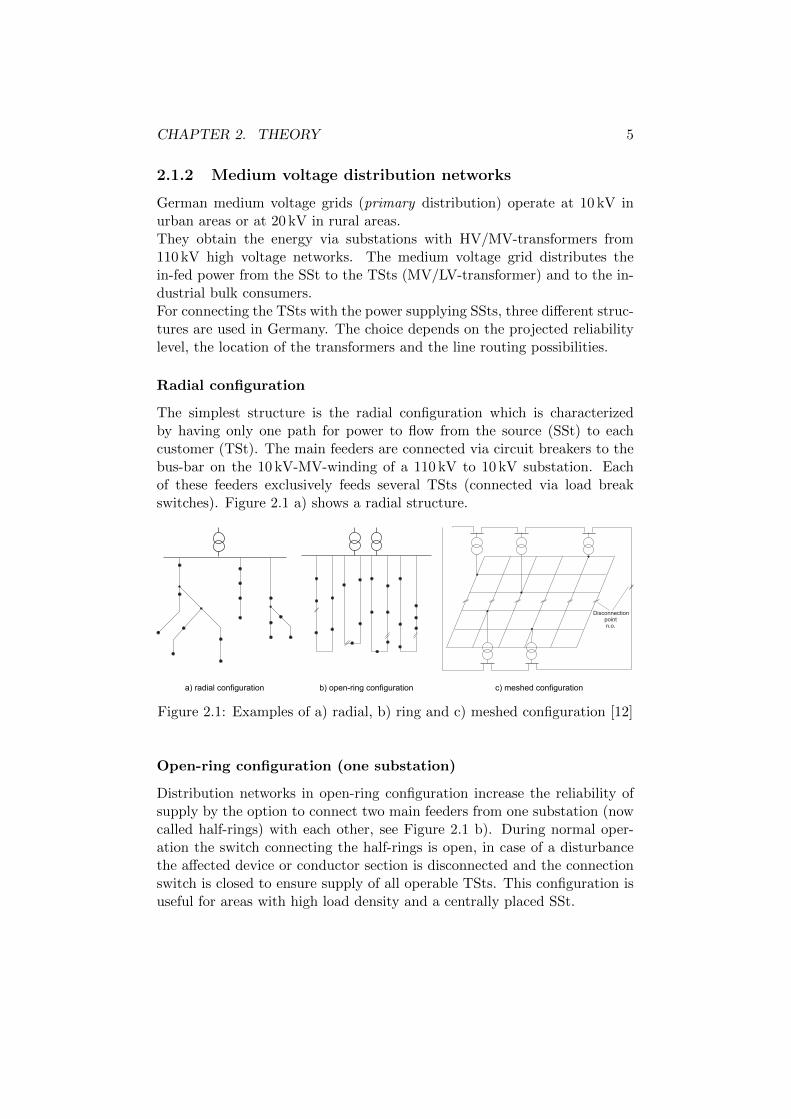
Radial configuration
The simplest structure is the radial configuration which is characterizedby having only one path for power to flow from the source (SSt) to eachcustomer (TSt). The main feeders are connected via circuit breakers to thebus-bar on the 10 kV-MV-winding of a 110 kV to 10 kV substation. Eachof these feeders exclusively feeds several TSts (connected via load breakswitches). Figure 2.1 a) shows a radial structure.
Disconnectionpointn.o.
a) radial configuration b) open-ring configuration c) meshed configuration
Figure 2.1: Examples of a) radial, b) ring and c) meshed configuration [12]
Open-ring configuration (one substation)
Distribution networks in open-ring configuration increase the reliability ofsupply by the option to connect two main feeders from one substation (nowcalled half-rings) with each other, see Figure 2.1 b). During normal oper-ation the switch connecting the half-rings is open, in case of a disturbancethe affected device or conductor section is disconnected and the connectionswitch is closed to ensure supply of all operable TSts. This configuration isuseful for areas with high load density and a centrally placed SSt.

CHAPTER 2. THEORY 6
Open-ring configuration (two substations)
In the cases of elongated areas, long straight cable routes or outlying SSts it isrecommended to construct an open ring structure between two different SSts.In this configuration the two half-rings start at two different neighboring SSt(which are connected via the HV grid). The switching procedure is similarto switching with only one SSt.
2.1.3 Low voltage distribution networks
German local low voltage grids (secondary distribution) operate at 400 Vand spread out from a single TSt (MV/LV).A TSt’s supply radius is between 250 m to 500 m depending on its ratedapparent power Sr (100 kVA to 630 kVA). This corresponds to 30 to 500residential units, the radius of the supply area is limited by voltage droplimits along the lines.In addition to the transformer, cable distribution cabinets with 4 to 8 outletsare placed at crossroads. This allows an individual disconnection of malfunc-tioning sub-feeders while the main feeder maintains normal operation.Although the reliability level decreases from meshed1 over open-ring to ra-dial configuration [11] the radial configuration is because of its easy andclear operation the most practical configuration [13, 1].
2.1.4 Reliability levels
According to [11] European distribution systems can classified by one out ofthree reliability levels:
Reliability level 1
• MV: each transformer is connected to the source through two feeders(one is a standby to the other)
• LV: one of the following configurations
– open-ring
– combination open-ring with double radial
– double radial supplied by a double TSt
– double radial supplied by two TSts
– closed-ring
– semiclosed-ring
• fast automation technique
1The meshed configuration completes the open-ring concept of double supply so thatall nodes and branches are connectable to multiple supplies, see Figure 2.1 c).

CHAPTER 2. THEORY 7
• backup generators to supply very critical loads
Reliability level 2
• MV: as for level 1
• LV: one of the following configurations
– open-ring
– combination open-ring with double radial
– double radial supplied by a double TSt
– double radial supplied by two TSts
Reliability level 3
• MV: as for level 1
• LV: Radial feeders. If a fault occurs on these feeders all load behindthe fault is disconnected.
As it was explained in the above sections, LV grids are preferably run inradial and MV grids in open-ring configuration.Comparing the three different reliability levels it is obvious that in all threecases, the MV connection must be at least in open-ring structure.The LV level can be realized in radial configuration for all three reliabilitylevels with the difference that for reliability level 1 and 2 the TSt has to beequipped with a standby transformer and a second standby line in parallelto the radially laid lines of reliability level 3.A distribution network consisting of radial LV structures and an open-ringMV structure can meet the requirements of each of the three reliability levelswithout modifying the topology (but doubling the transformer power andtotal line length).This network concept is chosen for this project in order to both avoid acomplicated structure and offer all three reliability levels at the same time.
2.1.5 Differentiation by geographic area
The load density of a supplied area has critical impact on the characteris-tics of the grid so that grid types can be differentiated by the regional loaddensity [13].Scheffler showed that specific load densities can directly be linked to certainsettlement patterns. In addition he identified characteristic variables for lowvoltage distribution grids for each of the defined settlement patterns [1].Some of these variables will be used for our generic distribution grids eitherfor the construction, as the rated TSt power, the number of feeders leaving

CHAPTER 2. THEORY 8
the station (Appendix A.2), or the verification of the model, e.g. length ofthe feeders, conductor material of the feeders, distance between connectedbuildings.However Scheffler’s settlement patterns only hold for areas between 6 ha to60 ha and their classification is done by only soft criteria.The Bundesinstitut fur Bau-, Stadt- und Raumplanung (BSSR) on the otherhand offers a classification of counties and regions by population density [14]allowing a better mapping of the regional observations made by [13] and [15].Using the number of housing units per connected building and the averagearea per building from Scheffler it was possible to merge each populationdensity class with its most common settlement pattern by Scheffler to sevenareal classes (ACls).The resulting ACl classification which is used in this project for modelingdifferent settlements is listed in Table 2.2 together with the BSSR classifi-cation and the assigned settlement patterns by Scheffler.Figure A.1 shows the map of the BSSR classification applied on Germany.
Table 2.2: Population density classification of different regions and the mostcommon settlement patterns
BSSR classification (modified)
settlement pattern by [1]arealclass area type (density) inhabitants
km2
scattered settlements R1 rural area (low) 0-100villages (mainly farms) R2 rural area (high) 100-1501- and 2-family houses area U1 urbanized area (low) 150-2001-family houses, village center U1terraced housing U1row development U2 urbanized area(high) 200-250block development A1 area with agglomera-
tion centers250-300
medieval old town A2 agglomeration 300-500high-rise row development A3 agglomeration (high) >500
Unfortunately it was not possible to properly analyze the statistical signif-icance of this classification using the DSO database due to the insufficientquality of the database. Determining the ACls’ statistical significance ishighly recommended as soon as a complete database is available.
2.2 Distribution grid components
In this section the models of the three most fundamental components of adistribution grid (1) Loads, (2) Lines and (3) Transformers are explained.For a complete description of a distribution grid further elements such as

CHAPTER 2. THEORY 9
Residential Commercial Industrial
Evening
Midday hours
Earlymorning
00
Pow
er d
eman
d
Pow
er d
eman
d
Pow
er d
eman
d
HourHour Hour
Figure 2.2: Most common DG load classes according to [11]
switches, shunt capacitors and voltage regulators as well as the phasing ofloads and transformers have to be included [16], but these elements are notconsidered in this projects’ basic approach of generating the fundamentalstructures of distribution grids.
2.2.1 Loads
A common modeling approach in literature is classifying loads (= electricityconsumers) by their typical power consumption over the day respectivelyover the year (t-P -curves). According to Sallam et al. the most used classesare residential, commercial (usually LV) and industrial (usually directlyconnected to MV) [11].Their fundamental differences are illustrated in Figure 2.2: For the residen-tial class, the peak is almost in the evening while for the commercial classit is at midday hours. The industrial class is approximately constant fromthe late morning until shutting down in the afternoon.
German DSOs use so-called standard load profiles (SLPs), normalized to1000 kWh/a, to forecast the LV consumers’ demands. These SLPs, providedby the German association of energy and water industries BDEW, cover the15 min consumption of one residential, seven different commercial and threetypes of agricultural customers. Figure 2.3 displays the most-used SLPsof each group. The residential and commerce group are similar to those bySallam et al. , the agricultural customers have high demand during the earlymorning and late evening. The BDEW does not provide a SLP for industrybut a continuous band profile.For the planning and dimensioning of grids the most important information
is the maximum power which lines have to transport and transformers haveto transform at a certain time. Consequently the very necessary informa-tion about loads is their peak power demand ppk, the power factor λ, whichis the ratio between apparent power and active power, their yearly energyconsumption E to deduce the average power demand and information aboutthe coincidence of the loads peaks (how much each single load contributesto the coincident peak demand at a specific instant of time). The followingtwo sections provide concrete numbers for the loads connected to the LV

CHAPTER 2. THEORY 10
Figure 2.3: standard load profiles by the BDEW for households (H0), com-merce (G0) and farms (L0)
and MV grid.
LV loads
For each of the seven different ACls a most common building type was iden-tified in Table 2.2. It can be assumed that each of these buildings representsone connection point and has one service lateral (connection to the feeder).This means that the grid“sees”every building as one single load with one sin-gle maximum demand and one specific yearly power consumption althoughthe building may envelope multiple households as can be seen in Table A.4.To model loads with both a certain variation and consistency this projectassumes that in each ACl only the most common building type is presentbut the number of households in every buildings hcp varies within a uniformdistribution.The typical households’ yearly energy consumptions2 Eh are listed by meanand standard deviation in Table A.3. As we already have a variation of thehouseholds the standard deviation of the yearly consumption is neglectedin this project and the mean values are rounded to 100 kWh so that totalyearly energy consumption Ecp for each class can be determined:
Ecp = hcp · Eh (2.1)
The range of hcp and the values for Eh are listed in Table 2.3.In literature a wide variation of the households peak demand can be found
2Average size of a household in Germany 2011: 2.02. Source: Statistisches Bundesamt

CHAPTER 2. THEORY 11
ranging from 1.92 kW to 30 kW. A comparison is shown in Table B.2.In this project a peak demand of 18 kW was chosen as a compromise be-tween the more popular publications [2] and [4] and because it is based ona very practical approach [17].Table 2.3 lists the ranges of the coincident peak demand per building ppk,18kWdepending of the number of households in the building according to the co-incidence calculation from [17].Furthermore an attempt was made to acquire the necessary data for mod-els of commercial (supermarkets, offices) and public (schools, town hall) LVloads. Due to the lack of statistical data (see also Chapter 5) this was notsuccessful and non-private consumers had to be omitted for this project.
Table 2.3: Load per household and ratio of households per building by ACl
R1 R2 U1 U2 A1 A2 A3
Eh [MWh] 3.0 3.4 4.0 1.9 2.7 2.7 1.7hcp
a [un. dist.] 1–2 1–3 1–2 4–14 5–15 1–11 10–80ppk,18kW [kW] 18–25 18–30 18–25 35–64 39–66 18–57 54–147
aThe data from Scheffer (Table A.4) was fit into a uniform distribution with integerendpoints with a maximum variation around the given mean |∆µ| ≤ 0.1µ.
MV loads
Literature does not provide useful information about size, amount and dis-tribution of public, industrial and commercial buildings in MV grids. Asneither general nor for the ACls-specific data was found this project canonly consider private loads connected to the LV grid and assumes the MVgrid to be free of loads.
2.2.2 Transformers
LV: Transformer stations
Three variables define a transformer in a distribution system map [5]: (1)the location of the transformer, (2) its rated power Sr in kVA and (3) howit is connected to the grid.
Location As explained earlier, the location on the transformer station(TSt) depends on the structure of the supplied area:In grids of compact structure the TSt is placed as central as possible to min-imize line length and thereby minimize the line losses and voltage drops. Inlarge meshed systems with multiple redundant transformers, they are placedat the nodes with the highest load density. Depending on the reliability level

CHAPTER 2. THEORY 12
Figure 2.4: Transformer station by Siemens. Left: LV switches, right: MVswitches and transformer [15]
the TSt consists of one operating and one reserve transformer both havingthe same rating and placed in the same station.In certain areas, for example valleys in the mountains or elongated villages,it is sometimes preferred to place two (or more) TSts which operate in open-ring configuration along the areas longer axis.As this project focuses on radial configuration in the low voltage level, it isthe best choice to place the transformer at a location which minimizes thedistance to all the connected nodes [15].
kVA rating Design and rating of transformers for distribution systemsare in general subject to the particular conditions of the respective suppliedarea (construction type, rated apparent power, rated voltages, . . . ) but inorder to have spare transformers and to provide cost efficient maintenanceon the LV level the number of different types and ratings is kept limited [12].The available transformer ratings (according to EN 50464 [18]) for differentareal classes are listed in Table A.1. In all but the two very rural classes630 kVA transformers are the most popular standard transformers in use.Larger transformers would have enough power to supply more customers butdue to the relatively low load density in German cities (compared to otherindustrialized countries) the voltage drop along the lines would violate theallowed power quality limits.As public LV transformers generally exhibit less than 4500 full-load hoursper year an economical operation is only possible by temporarily exceeding

CHAPTER 2. THEORY 13
the rated apparent power. Luckily time-periods of very high coincident griddemand and therewith the overloadings generally coincide with winter sothat the transformers’ lifetimes are not affected [12]. But literature valuesto the maximum overshoot over the rated power, by which the transformerapproximately can be dimensioned, differ:
1. TSts with less than 3500 full-load hours can be sized according to IEC60076-7: Smax
Sr= 150% [19]
2. transformers can be loaded with up to 140% of its rated power [20]
3. SmaxSr
= 120% [1]
For this project a compromise between the two smaller numbers is chosen,also because the households’ peak loads were set to a relatively small numberand to maintain a buffer for line losses. So transformers are dimensionedaccording to this condition:
Sr >Smax
1.3. (2.2)
In this formula Smax represents the maximum coincident load seen from thetransformer node.Using the maximum non-coincident load (the sum of the maximum loadsSh =
ppk,hλ of all n households) and a degree of simultaneous usage g∞ = 0.06
the estimated coincident load Smax is [12]:
Smax = (g∞ + (1− g∞) · h−3/4t ) ·n∑h=1
Sh (2.3)
Where ght = g∞ + (1 − g∞) · h−3/4t returns the factor to calculate a singlehousehold’s load share of the total coincident load of ht connected house-holds.As it can be seen in Figure 2.5 distribution transformers are designed formaximum efficiency at 50% to 70% for the above explained reason of fewfull-load hours [13]. This observation can be used as a secondary criterionfor sizing the transformer respectively in order to verify the sizing.
Connection The number of transformer terminals (feeders leaving thetransformer) depends on the transformer model. The average and standarddeviation of leaving feeders by ACl is listed in Table A.2.The number of feeders leaving the TSt does not vary much because thetransformers and lines have standard sizes, in urban areas the number offeeders ranges from 4 to 6 and in rural areas from 1 to 3 [1].

CHAPTER 2. THEORY 14
0.975
0.980
0.985
0.990
0.995
1.000
0.4 0.5 0.6 0.7 0.8 0.9 1.0
Relative loading in p.u.
Eff
icie
nc
y f
ac
tor
Figure 2.5: Efficiency curve of a LV transformer Sr = 630 kVA [12]
MV: Substations
For SSts in the primary distribution much less data than for TSts was avail-able. One reason is that SSts come in a much higher diversity because theyare built up modular (gas-insulated or air-insulated).Designs and ratings vary over a large scale depending on the local load den-sity, the number and the demand of connected MV consumers and the geo-graphic conditions (75 MVA to 250 MVA in urban areas, 20 MVA to 200 MVAin rural areas).
Location In the model by Rui et al. a possible locations for the HV/MV-transformer SSt is either the center or the corner of the supply area [7].For supply areas with relatively high load density the SSt is ideally placedcentrally and supplies the TSt via open-ring configuration [15].In this project different possibilities for the substation-placement are real-ized: (1) geographically centered between all loads (only TSts so far) (2)centered between loads by position and power demand (3) user defined po-sition.
Rating As mentioned above, the rating of SSts and the number of installedtransformers depends on the total demand.The number of loads connected via TSts to one SSt can be very large sothe coincidence is very low and the total load curve seen from the SSt isrelatively flat. Therefore transformers in SSts operate most of the time at100% of their rated power unlike TSts do [12]. Consequently the best wayto calculate the approximate necessary rating of the SSt is by calculating

CHAPTER 2. THEORY 15
the total coincident load of all connected households hs so that
Sr = hs ·18 kW
λ· (g∞ + (1− g∞) · h−3/4s ) (2.4)
with power factor λ = 0.9 and coincidence factor g∞ = 0.06.
Connection Post specifies a range of 5 to 30 connected TSts on each ofthe substation’s outgoing rings, increasing with lower load density (fromurban to rural) [21].The maximum number of TSts per ring is limited to 64 in Germany [22].The number of rings and terminals can be assumed to be unlimited in thisproject as substations are equipped with large bus-bars from where the ringfeeders start off.
2.2.3 Lines
Power lines are the elements that connect the customer loads with the TStrespectively the TSts with the SSt to transport electric energy. Substations,transformers and distribution cabinets were explained in the previous Sec-tions 2.1.3 and 2.2.2.In compliance with the general situation in Germany (LV: 88% Cable, 12%OHL; MV: 78% Cable, 22% OHL) it can be assumed in this project that alllines are aluminum underground cables.Service laterals, which connect the buildings to the feeders installed underthe adjacent road are not considered in this project due to the lack of rele-vant data and the phasing of the cables will be neglected (as for the loads).Consequently each cable is defined by (1) the starting and ending point (2)the resulting distance and (3) the conductor size. (1) and (2) depend onthe position of the loads and the routing (see Section 2.3), (3) is explainedbelow:
Sizing of the lines
The following steps describe a procedure to determine the conductor cross-section based on the recommendation of a Swiss cable manufacturer [23]:
1. Calculating the nominal current
IN =Smax√3 · U
(2.5)
U = concatenated nominal voltage [kV]: LV 0.4 kVSmax = transmission power [kVA].
2. Determining correction factors for laying (underground either in tub-ing or directly in soil, overhead) and shield grounding. For standardconditions the correction factor equals 1.
CHAPTER 2. THEORY 16
3. Identification of the necessary cross-section using current carrying ca-pacity tables.
4. Recheck the cross-section
• MV: The short-circuit current must not exceeds the short circuitcurrent capacity. If so a larger cross-section must be chosen:
ISC =SSC√3 · U
(2.6)
SSC = short-circuit power [kVA]
• LV: The voltage drop along the line must not exceed the allowedmaximum voltage drop. Otherwise a larger cross-section must bechosen.According to the European norm EN 50160, the maximum per-missible voltage variation ∆U at the end customers’ installationsis limited to ∆Umax < ±10% · UN [24]. When the customers’ in-stallations are unknown a maximum voltage deviation of 5% ·UNat the service lateral is a sufficiently conservative approximation[12].The additional voltage drop occurring directly at the transform-ers primary side should be accounted with additional 2% resultingin a voltage drop limit of 3% · UN for LV lines [13].
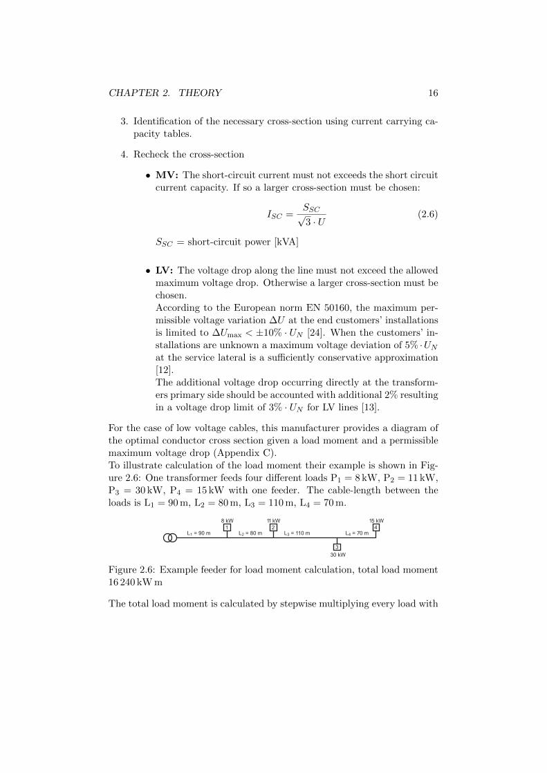
For the case of low voltage cables, this manufacturer provides a diagram ofthe optimal conductor cross section given a load moment and a permissiblemaximum voltage drop (Appendix C).To illustrate calculation of the load moment their example is shown in Fig-ure 2.6: One transformer feeds four different loads P1 = 8 kW, P2 = 11 kW,P3 = 30 kW, P4 = 15 kW with one feeder. The cable-length between theloads is L1 = 90 m, L2 = 80 m, L3 = 110 m, L4 = 70 m.
L1 = 90 m L2 = 80 m L4 = 70 m
8 kW 11 kW 15 kW
30 kW
1 2
3
4L3 = 110 m
Figure 2.6: Example feeder for load moment calculation, total load moment16 240 kW m
The total load moment is calculated by stepwise multiplying every load with

CHAPTER 2. THEORY 17
its distance to the transformer and summing these 4 load moments:
P1 · L1 = 720 kW m
P2 · (L1 + L2) = 1870 kW m
P3 · (L1 + L2 + L3) = 8400 kW m
P4 · (L1 + L2 + L3 + L4) = 5250 kW m
total load moment = 16240 kW m
Based on Appendix C the adequate copper cross-section for ∆U < 3% wouldbe Cu=95 mm2.
Line losses
Due to the lower voltage level in LV and MV networks the losses are muchhigher than in HV. They can be divided into three different types of losses:Ohmic losses, shielding losses and fuse losses.For the commonly used copper shielded cables up to 250 mm2 the ohmiclosses are much larger than both shielding and fuse losses. Accordingly thelatter two can be neglected in the loss calculation [23].The ohmic losses are
Pl = I ·R (2.7)
where R = R20 · (1 + α(T − 20 C)) and α = 0.00403 (aluminum).An approximation of line losses is not a task of this project but might bean interesting factor for later grid studies, therefore the ohmic resistance ofthe lines is calculated.
2.3 Power line routing
2.3.1 LV system
As discussed above, there a several different kinds of grid structures for thelow voltage systems but because of their simple operation radial networkswere and still are the most recommended structure. So this section coversthe routing of cables of a radial LV grid.For defining the supply area of a transformer and connecting the suppliedloads by cable the following criteria have to be considered:
• quality of power: Reduce voltage variations
• total costs: Investment in large cable cross-section against higheroperation costs by energy losses and aging of cables with smaller cross-section

CHAPTER 2. THEORY 18
• reliability/redundancy: Higher reliability means higher redundancyat higher costs. Trade-off between non-intermittent supply and largerinvestment for redundant technical devices. Three different reliabilitylevels are presented in Section 2.1.4.
Both voltage drops and energy losses are proportional to the length of theline and inversely proportional to its cross-section which was covered inSection 2.2.3. To keep investment costs low and avoid laying of unnecessaryline the minimum spanning tree algorithm, which minimizes the total lengthof all the low voltage grid’s cables, can be used.
Minimum spanning tree
The MST algorithm takes a connected undirected graph as input and returnsa tree which connects all the graphs’ vertices with the shortest possible totalline length and without any cycles.O. Boruvka was the first to formulate and solve the MST problem in 1926[25] while working on power grids. Several newer papers on distributionsystem design e.g. [26] recommend the MST to initialize a radial networkconfiguration.The popular MST solution by R. Prim is presented in Algorithm 1 [27].
Algorithm 1: Prim’s MST algorithm
Data: Connected weighted (e.g. edge length) graph with vertices Vand edges E
Result: VMST and EMST of MSTVMST = x, x is arbitrary vertex from V (root of tree), EMST = ;while VMST ⊂ V do
For u ∈ VMST and (v ∈ V ) /∈ VMST choose an edge u, v withminimal weight;Add v to VMST, and u, v to EMST;
end
Cluster analysis k-means
The voltage drop can not only be avoided by taking the shortest possiblepath to the load but also by reducing the direct distance between the con-suming load and the supplying transformer. For an area which has to besupplied by more than one TSt cluster analysis can be used to determinethe supplied area of each TSt.The k-means algorithm partitions n observations into k clusters so that eachobservation belongs to the cluster with the nearest centroid. The cluster’scentroid is the point to which the sum of distances from all objects in that

CHAPTER 2. THEORY 19
cluster is minimized (for advantages and limitations see [28]).In our case, the consuming loads are the n observations, the total number oflow voltage grids equals the number of clusters k and the centroid locationcan be used as the ideal location for placing the TSt.
2.3.2 MV system
For the medium voltage grid the same criteria as for LV grids should beconsidered: Quality of power, total costs and reliability. But for the mediumvoltage level a cost minimizing open-ring configuration is the structure ofchoice due to higher reliability requirements.As for low voltage, costs are approximately proportional to the total linelength so the problem becomes connecting all transformer stations to thesubstations in rings of minimum total line length.For the case of one single ring and one substation the problem equals thetravelling salesman problem (TSP) and the same solution algorithms can beused.
Vehicle routing problem
Two constraints interfere with the TSP approach: (1) keeping the distancebetween TSt and SSt short in order to minimize voltage drops and (2) com-plying with maximum number of TSts a ring-feeder can supply. To includethese two constraints it can be necessary to feed the TSts via different ringsfrom the substations.Allowing multiple rings (and substations) leads to the vehicle routing prob-lem (VRP) (with multiple depots). Bozic and Hobson provide an overviewof different approaches to these problems [29].In this project we assume that one single SSt feeds the transformer stationsvia different feeders where all feeders originate and terminate in the sameSSt so that the problem can be solved with standard VRP algorithms.
Sectioning of the ring
The MV grids in this project are operated in open-ring configuration. Inorder to guarantee reliable operation of the grid all line sections are equippedwith disconnectors so that faulty TSt can be disconnected while maintainingthe supply for all the other TSts.This set-up also demands a default sectioning point for normal operation.In this project the line which balances the sums of maximum demands onboth half-rings is chosen as sectioning point.Other possibilities would be balancing (1) the sum of the transformer ratingsor (2) the total length of the half-rings.

Chapter 3
Implementation
In this chapter, the Matlab-implementation of the module and its controlare explained. As in this project the grid generation is based on a spatialpopulation density map a graphical interface provides the user with thelayout of the grid and displaying options. The data structures which describethe grid are returned to the user in matrices.The module is invoked in Matlab with the command
[LV CP, LV L, MV CP, MV L, TD, S] = grid builder main GUI (3.1)
with a variable number of outputs, namely low voltage connection pointsLV CP, low voltage lines LV L, medium voltage connection points MV CP,medium voltage lines MV L, the data from the GUI table TD and furtherstatistics S.
3.1 Data
3.1.1 Input
In this Matlab implementation two types of input parameters are used.Fixed constants which are defined in fixed parameter.m (Table D.1) and theparameters loaded from the file user parameters.m. The user is advised toonly adjust the latter ones which are listed together with their default valuesin Table D.2.In addition to the pre-defined parameters the user has to choose between dif-ferent construction options during the construction procedure. The differentoptions offered in these dialogs are summarized in Table 3.1.
3.1.2 Output
The information and properties of the distribution grid’s components arestored in matrices and returned to the user for further evaluation after fin-ishing the construction of the distribution system model.
20

CHAPTER 3. IMPLEMENTATION 21
Low voltage connection points
For each independent low voltage grid both transformers and loads are storedtogether in a nodes-matrix and all these matrices of the independent gridsare put into the cell array LV CP.
Transformers In the first line(s) of the grid matrix the transformer(s) aredescribed by position xt and yt, the rated power Sr [kV A], the total numberof households connected to the transformer hSg, the maximum coincidentapparent power demand Smax [kV A], the yearly energy supply ESg [kWh]and the index of the sub-grid the transformer supplies Sg (see Section 3.3.2)in the following order:
[xt yt hSg Smax ESg Sr Sg]
As the number of independent LV systems is user-defined, it can occur thatthe maximum available transformer rating is not high enough to supply allloads in the specific system so it gets split up into multiple interconnectedsub-grids (Section 3.3.2). For this reason one LV system can have more thanone transformer.
Loads In the following lines of the matrix all system’s consumers are de-fined. Each row contains the position of a building’s connection to the feederxcp and ycp, the number of households per building hcp, the buildings coin-cident peak power demand at the connection point ppk [kW] the buildingsyearly energy consumption Ecp [kWh], the ACl of the pixel Dpx where it isplaced and the index of the sub-grid Sg, it belongs to:
[xcp ycp hcp pcp Ecp Dpx Sg]
The buildings coincident peak load is only relevant for cable sizing. Fortransformer dimensioning the total peak load is different from the sum ofthe buildings peak loads because (1) of a higher coincidence factor and (2)because of the line losses.
Differentiation To allow an easy differentiation of transformers and loadsyearly consumption is stored with a negative sign while the supply by thetransformer is positive (5th column).
Low voltage lines
The information about the connecting lines is stored row-wise in a line-matrix for each independent low voltage grid. This approach was preferredto the use of adjacency matrices because it eases handling each line as anobject. The relevant information about each line are the cable length l [km],

CHAPTER 3. IMPLEMENTATION 22
the start-node ns and the end-node ne (corresponding to the row in thenode-matrix), the index of the sub-grid it belongs to Sg, the cross-section ofthe line c, the ohmic resistance (operating temperature 50 C) of the line R[Ω] and their current operation state St (open/closed: 0/1):
[l ns ne Sg Sg c R St]
The open lines which are interconnecting possible sub-grids are stored belowthe closed lines. For the closed lines both the start sub-grid Sgs and the endsub-grid Sge are given:
[l ns ne Sgs Sge c R]
As for the nodes one matrix contains all the lines of one independent distri-bution grid. The line matrices of different independent grids are organizedin the cell array LV L.
Medium voltage connection points
This project assumes that one single SSt supplies the whole grid. Accord-ingly this SSt is described in the first row of the matrix MV CP by itsposition xs and ys, Sr the recommended rating according to Equation (2.4),the sum of the maximum coincident power demands of the transformersSmax, the total number of households in the LV grid and the total yearlyconsumption Es [MWh]:
[xs ys hs Smax Es Sr]
The TSts from the LV grids become loads in the MV grid and are listedbelow the SSt. The relevant information about these TSts are the positionxt and yt, their maximum power demand Smax, the number of householdsin the LV grid ht, the yearly consumption Et [MWh] and the Ring Rg theyare connected to:
[xt yt ht Smax Et Rg]
Medium voltage lines
The lines in the medium voltage (Matrix MV L) have the same specificationsas the LV lines except for two changes: Instead of the index of a sub-grid theindex of the ring Rg by which the load is supplied is given and furthermorethe operating state St (open/closed: 0/1) of the line is indicated:
[l ns ne Rg c R St]
CHAPTER 3. IMPLEMENTATION 23
Statistics
The statistics matrix S returns for each available low voltage cross section(row 1 to 9), medium voltage cross section (row 10 to 15) and transformerrating (row 16 to 21) its absolute (second column) and relative usage (thirdcolumn). The absolute usage of the cross sections is measured in km oflines but for the transformer ratings in deployed transformer stations. Therelative usage consequently is given in percent and calculated in relationto the overall line length respectively to the overall number of transformerstations.
Unit system
During project development the idea of using p.u. units instead of SI unitswas considered. Whilst the p.u. system is very useful for the qualitativeanalysis of an active power system (easier detection of gross errors, over-loading, . . . ) the SI units seemed to be more suitable as grid characteristicsare generally provided in SI units, as the necessary calculations are limitedto the dimensioning of lines and transformers and because no grid analysis(neither steady state nor transient) is performed.On the contrary the p.u. system would require a double conversion: The ini-tially given input parameters first have to be converted to p.u. for the gridconstruction but for comparison to literature they have to be in SI unitsagain.Hence SI units are used throughout the project.
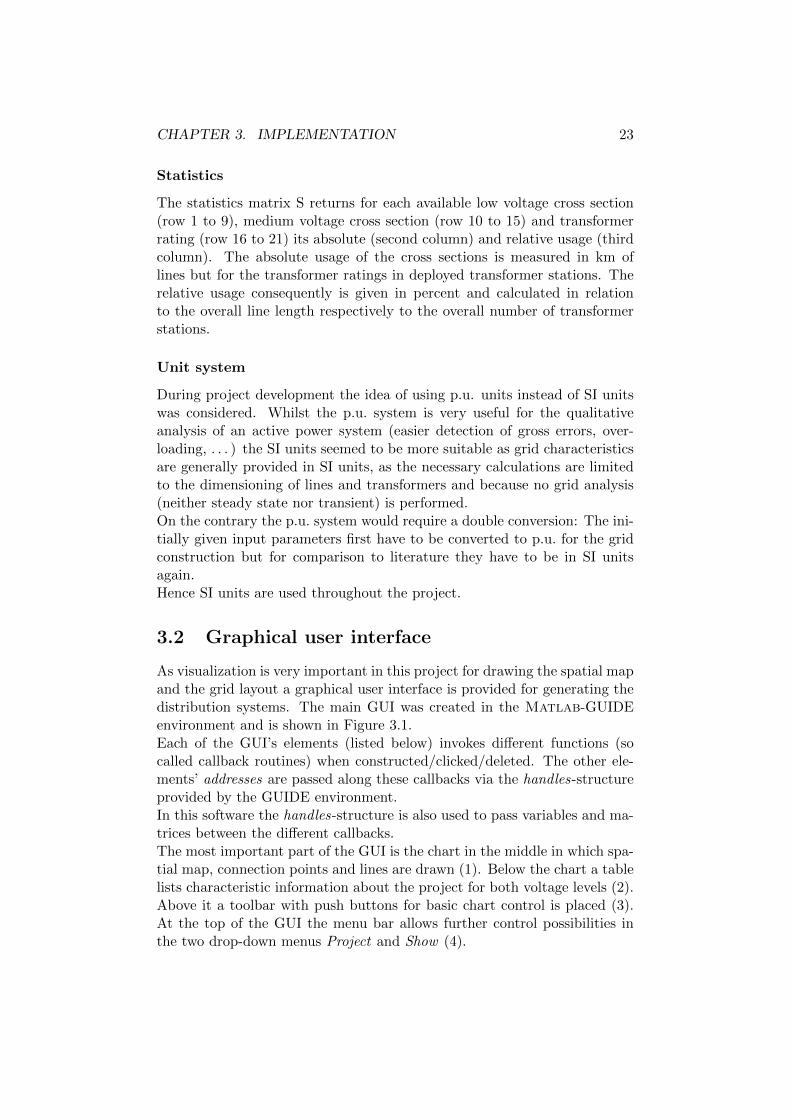
3.2 Graphical user interface
As visualization is very important in this project for drawing the spatial mapand the grid layout a graphical user interface is provided for generating thedistribution systems. The main GUI was created in the Matlab-GUIDEenvironment and is shown in Figure 3.1.Each of the GUI’s elements (listed below) invokes different functions (socalled callback routines) when constructed/clicked/deleted. The other ele-ments’ addresses are passed along these callbacks via the handles-structureprovided by the GUIDE environment.In this software the handles-structure is also used to pass variables and ma-trices between the different callbacks.The most important part of the GUI is the chart in the middle in which spa-tial map, connection points and lines are drawn (1). Below the chart a tablelists characteristic information about the project for both voltage levels (2).Above it a toolbar with push buttons for basic chart control is placed (3).At the top of the GUI the menu bar allows further control possibilities inthe two drop-down menus Project and Show (4).

CHAPTER 3. IMPLEMENTATION 24
Figure 3.1: Graphical user interface

CHAPTER 3. IMPLEMENTATION 25
3.2.1 Chart
The chart covers the largest part of the GUI and default it blank and scaledto 1× 1 km2.The chart’s size is linked to the size of the GUI so resizing the GUI directlyaffects the size of the chart.
3.2.2 Table
In the table the most relevant characteristics of the grid are updated dynam-ically during the construction phase. For both voltage levels the followingproperties are listed:
• Area [km]
• Inhabitants
• Settlements
• Connected loads
• Maximum power [kVA]
• Yearly consumption [MWh]
• Lines [km]
• Average CP distance [m]
• Transformers
• Installed power [MVA]
3.2.3 Toolbar
Seven pushbuttons which are placed above the chart area allow quick basiccontrol over the chart. The Menu Show offers further possibilities to adjustthe presentation of the distribution system area:
button function
save same as Save Project (Menu bar)zoom in zoom in by a factor of 2 with each mouse clickzoom out zooms out by a factor of 2 up to original sizedatacursor show exact coordinates of a selected datapointcolorbar display/hide the color legend on the right of the chartlegend display/hide the line and CP legendgrid display/hide grid lines on the charts top layer
3.2.4 Menu bar
The menu bar offers two drop-down menus Project and Show. The first oneprovides the basic start and save routine to initialize and end the projectwhilst the latter one contains tools to improve the network visualization.

CHAPTER 3. IMPLEMENTATION 26
Project function
New Project Initializes the construction of a distribution gridSave Project Allows saving the output data as (.mat) and the grid map
(.fig) to a personal folder via a dialog box
Show shown/hidden objects
Pop Centers Placed population centers and their labelsDensity map Density heatmapLV Loads position of buildingsMV Loads position of the TStsLV grid active and open lines of the low voltage grid & TStsMV grid active and open lines of the medium voltage grid & SSt
Initially it was intended to give the user the possibility to pause, saveand exit his current project at every dialog and to reload the saved dataand continue the project later. For this reason all steps described beloware embedded in a large switching-routine which allows an easy resumptionwith a known case-number.The save-open-concept was dropped at a later development stage when itbecame clear that the program works without computationally intensivealgorithms but some artifacts of the concept remained in the code, e.g. anopen-callback and the switching routine.
3.3 Generation of a distribution grid
In this section the distribution grid generation procedure is explained. Theprocedure is initialized by starting a new project from the menu bar Project→ New Project. The procedure is illustrated in Appendix D.3.
3.3.1 Modeling of a spatial load map
First an input dialog asks the user for the total area and inhabitants of thedistribution system. Then he is given the possibility to place populationcenters of different densities and size on a discrete quadratic map with auser-defined resolution (default 100× 100 pixel).Subsequently the user chooses a smoothing factor for the map in order toreduce the gradients between the different population centers.Based upon the pixels’ population density the ACl and the number andtype of connected building is determined for each pixel. In the next stepthe buildings are randomly distributed within the pixels and their electricityconsumption is chosen according to Section 2.2.1.
1. An Input dialog demands area A and number of inhabitants I

CHAPTER 3. IMPLEMENTATION 27
2. The map is discretized into 100×100 quadratic pixels each of size A10000
3. The user chooses the background density from 8 different densities.
• zero
• far-scattered (=R1)
• scattered (=R2)
• slightly scattered (=U1)
• fairly populated (=U2)
• slightly dense (=A1)
• dense (=A2)
• very dense (=A3)
These densities have to be seen relatively to (1) the total populationdensity given through I and A and (2) the density of the populationcenters placed in the subsequent step. Nonetheless the pixels’ valuesare set to a density drawn randomly from between the limits of theareal class corresponding to the chosen relative density.The map’s background takes on the color of the chosen backgrounddensity.
4. For each of the 8 densities the user can place c quadratic settlementcenters on the map which are immediately plotted in their color.The densities are defined the same way as they are in the second step,for each center there is one random draw of its density. The centers’sizes increases with density, for zero it is one pixel, for very dense thecenter extends 7 pixel in every direction to a total area of 15×15 = 225pixels.The population centers’ midpoints and areas are plotted into the map.
5. The user defines the smoothing out of the map on a scale from 0 to100 either via input field or by moving a slider with the mouse. Hecan directly see the effect of the smoothing in the map before he con-firms his choice. The higher the smoothing factor is set the more thequadratic centers become circular and larger.The used smoothing function smooth2a.m smoothes the data in a ma-trix M using a mean filter over a rectangle of the size (2sx + 1) ×(2sy + 1). It works like a two dimensional moving average where thevalue of the elements of the rectangle with center i is replaced by therectangle’s mean value. It was developed by G. Reeves [30].Several tests revealed that the best graphical results are achieved witha rectangle of size 3 × 3 (sx = 1, sy = 1) repeated up to 100 times(maximum resolution).
6. The smoothed map is linearly scaled up to meet the total number ofinhabitants I.The population Ipx and the density Dpx of each pixel is calculated, so

CHAPTER 3. IMPLEMENTATION 28
that the areal classes of the pixels AClpx are defined.Knowing the average number of households per connection point ofeach areal class (Table A.4) the software calculates the number ofconnected buildings in each pixel Ncp,px.
7. Using the density class Cpx and the number of buildings Ncp,px thesoftware defines the connection points:
(a) For each connection point CPi its x and y coordinates are drawnfrom an uniform distribution to randomly position the buildingwithin the pixel
(b) The number of households in each building is drawn from theuniform distribution over the range of households as given in Ta-ble 2.3.
(c) The yearly load of each building is the product of the averageyearly load of a household of the corresponding class (Table 2.3)and the number of households per building hcp.
8. The loads are plotted as black cross-marks onto the colored spatialmap.
The design of the spatial map and the smoothing effects are illustrated inFigures D.2 and D.3
3.3.2 Generation of the LV distribution grid
Clustering of low voltage systems
After the loads are plotted, the user has the possibility to set the number ofindependent (not interconnected) low voltage distribution grids. As default
Grec =ghs · hs · 18 kW
λ · 630 kVA · 1.3(3.2)
grids are recommended. Grec is calculated from the systems total coincidentconsumer peak load divided by the maximum permissible transformer power.Furthermore the software proposes a minimum and maximum number ofgrids calculated from the number of placed centers c, the number of ofconnection points connected to the feeders CPst and the maximum numberof connection points per transformer CPsmax :
Grec,min = max
(1,min
(c,
⌊CPst
CPsmax
⌋))(3.3)
Grec,max = max
(c,
⌊CPst
CPsmax
⌋)(3.4)
If the default value does not lie within these boundaries, it is to be adjustedto the closer one.

CHAPTER 3. IMPLEMENTATION 29
The user can ignore these recommendations and chose an arbitrary numberof independent low voltage grids g.In order to divide the area geographically k-means clustering is applied onall loads with k = g. For the resulting clusters the maximum linear distanceand the maximum average distance is returned to the user so that he canincrease or decrease g to initialize another run of k-means until he confirmshis choice.Finally, the identified centroid positions of each of the clusters are storedas the grids’ transformer locations and for each independent low voltagesystem the loads and transformers are sorted into a matrix as described inSection 3.1.2.The clustering dialogs and effects are illustrated in Figure D.4.
Connecting the LV components
For each of the independent low voltage systems Gi, i ∈ 1 . . . g, the followingsteps are implemented to connect the consumer loads to the TSts:
1. Necessary Sub-grids: If the load clusters do not fulfill the conditionsto ensure supply k-means clustering is executed on the grid Gi withincreasing k until the conditions are met. This way Gi is split up intosg = k interconnectable sub-grids. The conditions are:
• The largest of the available1 transformers (Table A.1) must belarge enough to approximately supply all ht households in Gi.The conditions approximates line losses with 5% of the coincidentpower:
1.25 · 630 kVA > ght · ht ·18 kW
λ
• The longest direct distance dt,cp from the transformer to any loadis shorter than the maximum distance allowed dmax(= 700 m).
maxcp∈CPs
dt,cp < dmax
When both criteria are fulfilled the node-matrix is updated by theposition and number of transformers (centroids) and the loads’ sub-grid indices SGj resulting from the above clustering.
2. Distance Matrix: The distance matrix of the nodes (transformersand all buildings) Di is calculated. The distances can either be calcu-lated in Euclidean (default) or cityblock metric (see Section 4.3.3).
3. Minimum spanning tree: For each sub-grid SGj the MST startingat the transformer ti,j is calculated.
1The average of the loads’ pixel ACl AClpx gives the sub-grid’s areal class AClSg

CHAPTER 3. IMPLEMENTATION 30
The MST implementation is based on Prim’s algorithm but modifiedwith regard to the number of transformer outlets:Based on the average ACl of the appendant loads the number of trans-former outlets OT is drawn from a normal distribution according to Ta-ble A.2. The OT closest loads are directly connected to the transformerand subsequently the minimum spanning tree is initialized startingfrom these OT + 1 fixed nodes. The resulting lines are then stored inmatrices as described in Section 3.1.2For each connection point m its degree a(m) (adjacent nodes) is stored:
• a(m) = 1: end point
• a(m) = 2: normal node
• a(m) > 2: junction2
4. Interconnection of Sub-grids: The user sets the maximum numberof interconnections of each sub-grid to other sub-grids lSgSg throughan input dialog once.For each sub-grid SGj the ljSg = min(lSgSg, sg) shortest connectionsto the other sg sub-grids SGk,k 6=j are searched and stored as an openline. To avoid repetitions the algorithm checks for already existingconnections between k and j.
5. Dimensioning the transformer: As default the transformers aredimensioned sub-grid-wise as described in Section 2.2.2 for the maxi-mum coincident load Smax. Smax is approximately calculated from thetotal number of supplied households and the coincidence factor.Then the density class specific transformers are compared to Smax andthe lowest rating fulfilling Equation (2.2) is chosen.The user can also choose a second option for dimensioning in the set-up: All transformers of interconnected sub-grids are rated with thesame power as the largest necessary transformer so that each trans-former can replace another one in case of an outage.
6. Dimensioning the lines: To initialize the calculation of the lines’cross-sections the end nodes (a = 1) of the grids are searched. Thena recursive search for each nodes parent is performed. Thereby theparent’s children cumulative load moment and their cumulative loadis stored in the parent’s data and based on these, the cross-sectionand the according resistance of the line is determined as described inSection 2.2.3.At a junction, the recursion is paused until all the children of the junc-tion node have been evaluated. This is done by a second degree-indexfor each node which is reduced by 1 if an appendant line is dimen-sioned and recursion is only possible if this index equals 1.
2Real loads are not placed directly at junctions/cabinets but within meters distance.

CHAPTER 3. IMPLEMENTATION 31
In case the sub-grids are interconnected the interconnecting line ele-ment connecting two sub-grids l,m are dimensioned by an approxi-mated load moment
loadmoment = mink∈[l,m]
Smax,k · dist(i, j) (3.5)
resulting from the maximum coincident power demand (Equation (2.3))at the smaller of the two transformers times their line distance.Then recursively all line element between the connection points of theopen line and the TSts are sized accordingly.
7. Plotting the network: The sub-grids’ power line structure is plot-ted into the map as black straight lines. The open interconnectionsbetween the sub-grids are shown as dotted red lines. The TSts areplotted as yellow circles.
The LV grid design steps are shown in Appendix D.5.
3.3.3 Generation of the MV distribution grid
As described in Section 2.3.2 one single SSt supplies all existing TSt. Ac-cordingly the following steps only have to executed once:
1. MV matrix: Iteratively the relevant TSts’ data is extracted from theLV matrices and stored in the MV matrix.The total number of households in the network, the total yearly energyconsumption and the sum of the TSts’ maximum demands are storedin the first row of the MV matrix. The substation rating is calculatedaccording to Equation 2.4.
2. Placement of the substation: Via dialog box (Appendix D.6) theuser can choose between four different options to place the substation:
• by mouse-click
• geographic center of the map
• geographic mean of the TSt
• geographic mean of the TSt weighted with their maximum loading
The (calculated) substation’s position is saved in the MV node-matrix.
3. Identifying the ring configuration: The user-set parameter for themaximum number of TSt per ring Trg,max defines the number of rings:
nrg =
⌈nT
Trg,max
⌉(3.6)

CHAPTER 3. IMPLEMENTATION 32
The user is offered the option to balance the number of TSts per feeder.If activated the new maximum number of permissible TSts is set to
T∗rg,max =
⌈nTnrg
⌉(3.7)
In practice reducing Trg,max may corrupt the minimization of the totalline length. Together with this project’s non-optimal Vehicle Routingimplementation the default constraint will result in one ring which isdistinctly smaller (less TSts) than all other rings, the balanced con-straint on the other hand leads to rings of same size (equal number ofTSts).
4. Vehicle routing problem: After calculating the distance matrixfrom the TSts’ and the SSt’s positions the VRP algorithm is executed.In this module’s version a VRP script (Algorithm 2) based on the
Algorithm 2: VRP nearest neighbor
Data: Distances Ds,e between TSts (and the SSt), Tmax maximumnumber of TSts per ring
Result: nrg Matrices each containing start and end nodes and lengthof all line elements of the rings
Tunconn ← [TS1 . . .TSnT ];
nrg ←⌈#Tunconn
Tmax
⌉;
for r ← 1 to nrg dos← SSt;while #Tunconn > 0 & lines(r) < Tmax + 1 do
find closest e in Ds,e;store line ls,e;s← e;
endfind and store line ls,SSt;
end
nearest neighbor algorithm is implemented. The algorithm is veryquick but does not achieve an optimal solution. More sophisticatedalgorithms might be implemented in later versions (see section 4.4.3).
5. Dimensioning the lines: The necessary cross section for the linesis calculated ring-wise. For each ring the total coincident load mo-mentum (based on the TSts’s maximum coincident power demands)is calculated from both sides of the ring assuming the opposite con-nection to the substation to be open. Then the cross-section matchingboth this maximum coincident load and the user-given voltage drop

CHAPTER 3. IMPLEMENTATION 33
limit is stored for all line elements.The resistance of each line element is calculated and stored.
6. Locating the sectioning point: As described in Section 2.3.2 sev-eral possibilities to open the ring exist. The user can choose betweenbalancing by (1) transformer ratings (2) line length or (3) peak de-mand (households).In all three cases ring-wise matrix calculations are performed to mini-mize the difference between both half-rings. For (1) and (3) the respec-tive transformer properties f(·) are relevant so the last transformer ton the half-ring before the separation is identified by:
mint∈1...nt−1
∥∥∥∥∥∥t∑
j=1
f(j)−nt∑
j=t+1
f(j)
∥∥∥∥∥∥ = mint∈1...nt−1
∥∥∥∥∥∥2t∑
j=1
f(j)−nt∑j=1
f(j)
∥∥∥∥∥∥(3.8)
For the lines-criterion (2) the line element li+1 which will be discon-nected must not be included:
mini∈1...nl−2
∥∥∥∥∥∥i∑
j=1
lj −nl∑
j=i+2
lj
∥∥∥∥∥∥ = mini∈1...nl−2
∥∥∥∥∥∥2i∑
j=1
lj −nl∑j=1
lj + li
∥∥∥∥∥∥ (3.9)
The above optimizations are only applied for rings with at least 3connected transformers (4 lines). In the case of only one TSt the firstof the two identical connections is activated, in the case of two TStsthe line connecting the two transformers is disconnected.
7. Plotting the network: The MV lines are plotted similar to the LVlines but thicker. The SSt is plotted as a green circle.

CHAPTER 3. IMPLEMENTATION 34
Table 3.1: Overview of user dialogs
Dialog User input
Grid area Define area [km2] and population
Population Map Choose density levels (Section 3.3.1) for· Background density· Population centers
Smoothing Set smoothing factor for the map (0 to 100)
LV grids Set number of independent low voltage grids
LV voltage drop Define voltage drop maximum (1% to 7%)
Interconnections Set number of interconnections between sub-grids
Transformer rating Set transformer rating calculation method so thatit can fully supply· Its own Sub-grid· The largest connectible Sub-grid
Substation placement Choose placement method· calculation
- center of map- geographic center of TSts- rating-weighted center of TSts· mouse
Units per Ring Decide allocation of TSts to Rings· maximum: fill rings up to maximum· balanced: balance TSts per ring
MV voltage drop Define voltage drop maximum (1% to 7%)
Ring sectioning Set ring sectioning method. Calculate sectioningpoint by balancing half-rings’· TS rating· TS peak loading

Chapter 4
Results and discussion
In this chapter the (1) load map, (2) LV distribution system and (3) MVdistribution system outputs and layouts resulting from different testing setsare evaluated and the characteristics are compared to literature and refer-ence data. Furthermore the measured computation time of each of the threemain steps is discussed shortly and improvement potential regarding thesoftware functionality is discussed.The functionality of the module was tested with very basic map set-ups con-sisting of one single center of the same density as the background only scaledwith regard to population and area. This is necessary to avoid differences inthe testing spatial maps originating from the design procedure which doesnot yet allow the identical reproduction of more complex spatial maps.
4.1 Testing device
All computation time measurements were performed on the following device:
Device Lenovo X220
Processor Intel i7-2620M 2.7 GHz Quad-coreMemory 16 GB DDR3-RAMHard drive 256 GB mini PCIe SSDOperating System Windows 8.1 Pro 64bitMatlab R2014a 64bit
4.2 Spatial load map
The construction of the spatial load map was inspired by the JavaScriptheatmap script by P. Wied [31].As the implementation of a dynamically evolving heatmap by continuouscursor querying and simultaneous plotting of the resulting map into Matlab
35

CHAPTER 4. RESULTS AND DISCUSSION 36
was assessed as exorbitantly time consuming (more than one week) the sim-pler approach of stepwise center-placement was chosen.The load map design procedure is described in Section 3.3.1. As no othersoftware of similar functionality is known the procedure and the results areassessed only qualitatively.During software testing different observations on the behavior of this proce-dure were made which are outlined in the following section.
4.2.1 Results
Construction of the map
The implemented design procedure controls allow the construction of sketchypopulation density maps. Although it is quite difficult in the beginningroutine may enable the user to draw precise density maps (see also Sec-tion 4.2.3). For distribution systems of realistic scale (at least one largetransformer fully loaded, >1000 inhabitants, see Table 4.1) the differentACl of the pixels affect the randomized positioning of loads sufficiently sothat different load densities are visible to the naked eye.
Table 4.1: Maximum number of households and inhabitants supplied by astandard transformer
Sr [kVA] hh inh.
50 20 40100 64 129160 121 244250 211 426400 364 735630 604 1220
Connection points
The DSOs’s database has an average of 1.95 persons per LV CP. As thisnumber also includes commercial and industrial CPs the general validity ofboth the assumption of 2.02 persons per household (German governmentalstatistics) and the resulting density of CPs can neither be rejected nor con-firmed.In order to evaluate the connection point density a test map with 100000inhabitants was designed for each ACl (the area was set to match the ACl’saverage population density, see Appendix A.3). The resulting CP density iscompared to the DSO dataset density in Table 4.2.We observe that the test results behave antitonically and differ strongly fromthe monotonically increasing reference values. But surprisingly a strong

CHAPTER 4. RESULTS AND DISCUSSION 37
Table 4.2: Comparison of CP density from DSO database and softwareresults
R1 R2 U1 U2 A1 A2 A3
reference CP density [/km2] 42 68 95 122 147 216 613test CP density [/km2] 19 31 58 12 13 32 12
test household density [/km2] 29 61 86 104 132 193 526
compliance of the tests’ household density and the reference CP density ex-ists.This is either explained by a relative increase of non-private connectionpoints (bureaus and commerce buildings) inversely proportional to the rel-ative change of the CP density or by non-precise information in [17] and [2]about the collective usage of service laterals and CPs of row- and apartmentbuildings.
4.2.2 Load computation time
After the density map design the calculation of the pixels’ ACls and thenumber of buildings on each pixel follows before these buildings’ positionsand number of households are drawn from random distributions.In two test series with an increasing number of inhabitants (logarithmic:1, 5, 10, . . . , 500000, 1000000) on maps of 1 km2 respectively 100 km2 theload computation time was measured for the basic case of very scatteredbackground and one single very scattered population center in the center ofthe map. Independent of the number of inhabitants the computation timecommuted between 0.68 s to 0.77 s around a mean of 0.74 s.For maps with more than one population center with a density different fromthe background density higher computation times up to 1.4 s were observed(e.g. for the map in Appendix D.3: 1.34 s).For both the standard case and the case with a high population and manydifferent centers the computation time is short and does not demand theusers patience.
4.2.3 Scope for improvement
Relative density colors vs real density colors
Observation For a small number of population centers the population-corrected background density color may differ considerably in color fromthe originally chosen background density (Figure 4.1).
Explanation The reason is obvious, an example: The relative backgrounddensity is set to scattered but the user-defined area and inhabitants result in

CHAPTER 4. RESULTS AND DISCUSSION 38
Figure 4.1: Density map before (left) and after (right) smoothing and scal-ing. Area 10 km2, inhabitants 3000, smoothing factor 10
an average of 800 inhabitants/km2 so the background is scaled up to arealclass A3 (light green becomes dark gray).
Possible solution This problem could be avoided by choosing differentcolormaps for each the relative densities during the construction phase andthe real densities resulting from the smoothing.Furthermore the real densities could be illustrated with a color gradientwithin each class.Another possibility is to allow the user to choose between two different colormaps (1) the nine class-colors or (2) a high resolution gradient of populationdensities.A thoughtful user will be able to use this software without getting confusedby the mapping of colors during these two phases of the spatial map design.Therefore modifying the colormap is of low priority only.
Hidden effect of smoothing
Observation For a high overall population density (above A3) the doesnot see effects of the smoothing as the whole map is painted in the samecolor even if different population centers densities and a low backgrounddensity was chosen as illustrated in Figure 4.2
Figure 4.2: Hidden effect of smoothing (10 km2, 100000 inh.): center place-ment (left), smoothing (middle), CP distribution (right)

CHAPTER 4. RESULTS AND DISCUSSION 39
Therefore the user gets the impression that changing the smoothing has noimpact on the spatial densities.
Explanation The areal class A3 covers all population densities above500 inhabitants
km2 so for a high enough average population density all pixels (eventhe very scattered ones) of the map are scaled up to ACl A3 and accordinglythe whole map appears dark gray for all smoothing levels.Nevertheless the pixels do have different population densities based on theratio between their relative densities chosen during map design.A high smoothing factor flattens these differences out while a low smoothingfactors leaves them more untouched.In any case differences in the densities become visible through the position-ing of loads which are shown after confirmation of the smoothing.
Possible Solution As for Problem 4.2.3 the easiest solution is introducinga color gradient within each areal class.The user has no possibility to find the effects of the smoothing factor butby guessing and testing so the implementation of this solution is of highimportance.
Decreasing building density with increasing areal class
Observation The density of connection points decreases in large steps be-tween some ACls while the population density increases. Especially betweenthe classes A2 and A3 the phenomenon is eye-striking (as in Figure D.5).
Explanation This observation may come surprising at first glance but islogically explained by the class specific average of housing units per con-nected building (Table A.4) which is not proportional to the increase ofpopulation density.Table 4.3 lists the expected building densities Buildings
km2 = pop. densppl/unit ·∅
unitsbuilding
for the different ACls. Between U1 and U2 and between A2 and A3 re-markably drops of building density occur which are reflected by the aboveobservations.In reality the ratio of built-up area to empty space is higher in U2 than in U1(and in A2 higher than in A1) because the building size increases stronglywith increasing areal class (a row development building needs much morespace than a 1-family house, see [1]).
Possible solution In order to avoid the user’s surprise about the morescattered connection points in pixels of higher density a possible solutionwould be using another connection point symbol (e.g. rectangles) with in-creasing size for the different building types. This way the plot of load

CHAPTER 4. RESULTS AND DISCUSSION 40
Table 4.3: Maximum and minimum of expected buildings/km2 for each arealclass
ACl R1 R2 U1 U2 A1 A2 A3
max. Buildingskm2 38 41 71 15 16 43 60a
min. Buildingskm2 0 28 53 12 13 26 6
aA population density of 5000 /km2 is assumed
connection points would better illustrate the real building situation.A simple Matlab implementation could plot the loads depending on theirACl with ACl-specific ’MarkerSize’ -values as square-markers ’s’ and the fillcolor ’MarkerFaceColor’ set to auto’. But as (1) a square area would repre-sent some building types inadequately (e.g. row buildings) and (2) the sizeof the markers remains constant throughout zooming this approach wouldbe only superficial.It is not the project’s aim to model building structures of population areasbut to model distribution grids so the visualization of the building densityis of very low priority.
Time-consuming drawing of centers of custom size
Observation In order to create ACl areas of custom size and shape theuser has to (1) either place multiple centers of the same category close toeach other to increase the size of the area or (2) place background-densitycenters close to the area in order to reshape or scale down the area.This is (a) very time consuming, (b) fault-prone because the size of a centeris not visualized before the placement and (c) the software is unforgiving assteps made are irreversible.
Explanations The distribution grids designed by this software are notrequired to be real but only realistic at this stage of development. For thisreason only the basic design steps with population centers of different densi-ties (and size increasing with density) were implemented and they producethe desired results. A more sophisticated map design was not intended dur-ing development.
Possible Solutions Highest priority of the three observations made is (c)the irreversibility. Consequently an Undo-Button was added to the Popula-tion center placement-menubar in parallel to the composition of this section.To resolve the scaling and shaping problems ((a) and (b)) possible solutionscould be implemented:

CHAPTER 4. RESULTS AND DISCUSSION 41
• The size of the placed center is predefined through user input beforeplacement (only (a), relatively simple)
• Within Matlab a drawing palette with draw and fill options is imple-mented to allow the drawing of individual maps (very and unnecessarycomplicated)
• The user can load a bitmap file of the population heatmap into Mat-lab which is then used for the load placement calculations (compli-cated (especially to match the colors) but feasible).
A solution to the problem of not displaying the expectable size of the centersbefore placement is not available as the Matlab-function ginput does notprovide an option to modify the cursor visualization.
Unimportance of relative densities in small maps
Observation For maps with small area the load positions seem to beunaffected by the population centers’ and the background’s density as shownin Figure 4.3.
Figure 4.3: Density map before (left) and after (right) smoothing and scal-ing. Area 1 km2, inhabitants 200, smoothing factor 50
Explanation This observation is not caused by errors in the algorithmbut can be explained by the very small area each pixel represents. The totalnumber of buildings is apportioned to all the pixels so that for each pixela probability for a building placed on this pixel can be calculated. For thevery small pixels’ area this probability relatively outweighs the differences inpopulation densities and the loads appear to be distributed totally randomly.
Possible Solution If the user wants to achieve a stronger placement ofloads by population density differences he is advised to choose a zero back-ground density and to place small population centers at the locations wherethe loads shall appear.
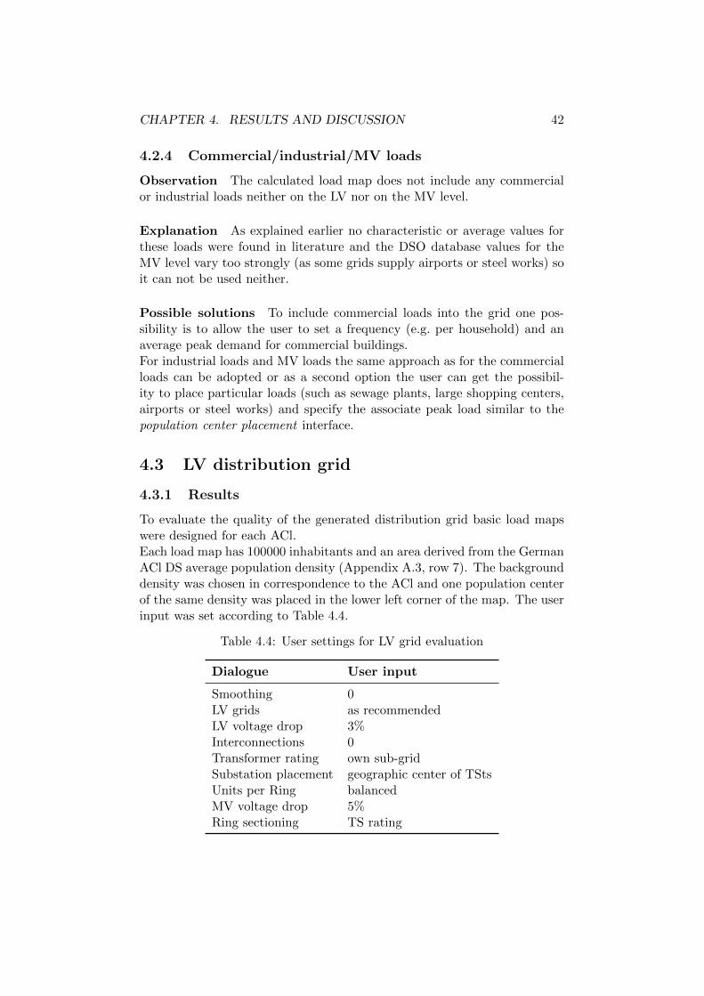
CHAPTER 4. RESULTS AND DISCUSSION 42
4.2.4 Commercial/industrial/MV loads
Observation The calculated load map does not include any commercialor industrial loads neither on the LV nor on the MV level.
Explanation As explained earlier no characteristic or average values forthese loads were found in literature and the DSO database values for theMV level vary too strongly (as some grids supply airports or steel works) soit can not be used neither.
Possible solutions To include commercial loads into the grid one pos-sibility is to allow the user to set a frequency (e.g. per household) and anaverage peak demand for commercial buildings.For industrial loads and MV loads the same approach as for the commercialloads can be adopted or as a second option the user can get the possibil-ity to place particular loads (such as sewage plants, large shopping centers,airports or steel works) and specify the associate peak load similar to thepopulation center placement interface.
4.3 LV distribution grid
4.3.1 Results
To evaluate the quality of the generated distribution grid basic load mapswere designed for each ACl.Each load map has 100000 inhabitants and an area derived from the GermanACl DS average population density (Appendix A.3, row 7). The backgrounddensity was chosen in correspondence to the ACl and one population centerof the same density was placed in the lower left corner of the map. The userinput was set according to Table 4.4.
Table 4.4: User settings for LV grid evaluation
Dialogue User input
Smoothing 0LV grids as recommendedLV voltage drop 3%Interconnections 0Transformer rating own sub-gridSubstation placement geographic center of TStsUnits per Ring balancedMV voltage drop 5%Ring sectioning TS rating

CHAPTER 4. RESULTS AND DISCUSSION 43
The resulting characteristic parameters shown in Table 4.5 are normalized byeither area or connection points to enable comparison to the DSO databasenumbers in Appendix A.3.It has to be noted that the data in Appendix A.3 results from real gridswith (1) commercial and industrial loads on both voltage levels and (2)comprises grids of different configuration (radial, open-ring, meshed) andtherefore certain discrepancies especially regarding the line length and thetransformer rating have to be expected.
Test grid results
Compared to the DSO database the following observations are made:
Inhabitants per CP The averages of inhabitants per connection pointdeviate strongly from the database numbers. The latter ones are very closeto the assumed average of 2.02 inhabitants per household. This is an in-dication to assume that the connected units listed in the DSO databasecorrespond to households.
CP density The connection point density calculated from the test resultsdiffer considerably from the database values:
• The test results for R1 to U1 have around half the density of thedatabase numbers. This might be explained with commercial loads.
• For the ACls U2 to A3 the density is differ strongly from the databasevalues (factor 10 to factor 30). As mentioned in Section 4.2.1 this ismost likely explained with the possibly wrong assumption of sharedCPs in apartment buildings.
Household density The household density matches the database’s CPdensity very closely (±10%). This observation strongly supports the thesisof non-shared CPs.
CP line distance The average distances between two connection pointsvaries between 100 m to 200 m and exceed the distances provided by Scheffler(Table A.6) by a factors between 4 to 20. The discrepancy between thesemeasured characteristics and those provided by Scheffler has most probablythe same explanation as the CP density results.
Line length per connection point The average line length per con-nection point exhibits the same precision pattern as the inhabitants perconnection point:

CHAPTER 4. RESULTS AND DISCUSSION 44
Tab
le4.
5:R
esu
lts
ofth
eLV
grid
eval
uat
ion
R1
R2
U1
U2
A1
A2
A3
inhabit
ants
/CP
3.03
4.04
3.41
19.9
520
.32
12.1
588
.18
CP
den
sity
[/km
2]
1931
5112
1332
12hh
den
sity
[/km
2]
2961
8710
413
419
352
6
CP
line
dis
tance
[m]
159
129
9421
120
414
020
6lin
es/C
P[m
]67
4023
9182
3514
0lin
es/A
[km/km
2]
3.1
4.0
4.8
2.6
2.7
4.5
2.4
ener
gyden
sity
[MW
h/km
2]
8620
932
320
136
152
087
0en
ergy
per
CP
[kW
h]
4505
6794
6282
1623
627
000
1624
273
690
pow
er/C
P[M
VA
]4
4.15
4.07
23.8
34.0
510
.04
90.9
1p
ower
/hh
[MV
A]
2.66
2.08
2.41
2.83
3.4
1.67
2.04
avg.Sr
[kV
A]
100
160
250
400
630
400
630
hh
/tr
ansf
orm
er37
7710
413
918
524
030
8C
P/tr
ansf
orm
er25
3961
1719
407

CHAPTER 4. RESULTS AND DISCUSSION 45
• For the ACls R1 to U1 the mean line lengths are relatively close to thedatabase values (±10 m).
• For U2 to A3 an increase in line length per connection point is observedin the test results whereas the length decreases for the database data.
The mishandling of the CPs/households connection issue may explain thedeviation for the ACls U2 to A3
Line length per area The line length per area measured in the test gridsis relatively close to the DSOs’ information but surprisingly the resultinglength for U2 and A1 are closer to the dataset for R2 and U1 and vice versa.The first of these two cases (relatively few lines calculated for U2 and R1)can partly be explained by the omission of inter-grid connections used morefrequently in areas of higher density.In the database the line length per area of ACl A3 stands out (11.1 km/km2)from the other ACls. Either the fact that many aged German DS are stillconfigured as meshed operation structure and therefore have more line-kmor this number is caused by corrupted data.
Transformer power per CP For the connection point specific trans-former power matching numbers can be observed for R1 to U1 but widedifferences occur for the remaining ACls.Possible reasons for the differences of the upper ACl were mentioned alreadyin previous paragraphs.
CPs(/households) per transformer The average number of loads sup-plied by a TSt was not given in the DSO database. But the average trans-former loading can be compared to the calculated maximum values listed inTable 4.1. For all ACls the average number of connected households is onlybetween 40% and 70% of the maximum connectible households.For the low density ACls this non optimal transformer utilization might bedue to the maximum transformer radius. The TSt utilization in high densityACls might be imperfect because of the large demand of the ACl’s buildings.See also section Overloading of transformers further below.
Main-feeder length Although Scheffler ([1]) provides information aboutthe average main-feeder length this characteristic is not calculated duringgrid construction because some main feeders are unproportionally short (seeSection 4.3.3).From the coding perspective a later implementation is simple: Using recur-sive search the longest possible paths starting from the feeders first node areidentified.

CHAPTER 4. RESULTS AND DISCUSSION 46
Cable cross section
Kerber provides data about typical cross-sections used in German rural andsuburban distribution systems and states that each feeder (and sub-feeder)has the same cross-section for all its length. In this project the optimal cross-section (except for the interconnecting lines) is calculated and dimensionedsegment-wise (the real approach is not implemented yet). For this reason itis pointless to compare the cross-sections resulting from the grid constructionprocedure with the literature values in [2, cp. 5.1.2.2.].On the other hand several test runs of the dimensioning procedure resultedin errors when no cross-section fulfilling the load moment and voltage dropdemands existed. This error was caught by dimensioning the respectiveline section with the largest cross-section available and recording the linedimensioning violation event.For a maximum voltage drop ∆V = 3% the number of violations normalizedby the number of TSts ranged between 15 to 20 for the ACls R2, U1 andA2. For R1, U2 and A1 between 8 to 10 violations per TSt were registeredand for A3 around 3 violations occurred per TSt. These observations matchwith the lines per area and the connection points density (Table 4.5) so theone reason for the line violations is the distance between the buildings whichstrongly affects the load moment. Another reason is that the load moment iscalculated based only on the buildings peak load and a flattening of the peakcurrent along the line due to non-coincidence is not taken into account.Increasing the maximum permissible voltage drop ∆V to 7% reduces thefrequency of violations for all classes by 65%.
Overloading of transformers
While testing the module the observation was made that some transformersin A3-networks were overloaded. This phenomenon can be explained by thevery large consumers in A3 and is therefore restricted to this ACl:During the grid construction procedure the number of sub-grids is calculatedusing the k-means algorithm. Iteratively for every sub-grid the necessaryconstraints (peak loading and load distance) are checked until met.After every check k is increased by 1 under the approximate assumption thatadding another cluster never increases but only reduces the peak loading andload distance in each cluster. This assumption does not hold properly forA3 as it can happen that one of the analyzed sub-grid’s large consumers isassigned to an already checked sub-grid while performing the next clustering.As the sub-grid conditions are not checked a second time after the iterationthe overloading of transformers can occur.Up to now the overloading violations are only registered. In later moduleupdates a computing-efficient constraint verification for all sub-grids aftereach clustering step can be taken into consideration.

CHAPTER 4. RESULTS AND DISCUSSION 47
4.3.2 LV grid computation time
During the construction of the test grids the computation time listed in Ta-ble 4.6 was measured. The computation time decreases with the decreasingnumber of connection points and as it can be seen in Table 4.6 the calcula-tion time per CP or per TSt only varies in the range of ms.This observation can be explained by the complexity of the k-means algo-rithm O(nk+1 ·log n) and the complexity of the MST algorithm O(l+n·log n)(number of loads n, number of lines l).
Table 4.6: Computation time for the construction of the LV test grids
R1 R2 U1 U2 A1 A2 A3
avg. calculation time [s] 70 25 20 25 17 9 12calculation time/CP [ms] 2.15 1.05 0.63 4.15 3.47 1.03 10.76calculation time/TSt [ms] 53 41 39 69 64 41 74
4.3.3 Scope for improvement
Edgy cable routing
Observation During software testing the edgy cable routing attractedattention. In practice cables routes are mainly laid below roads and followtheir course but different to the real situation where most crossroads and sideroads branch off perpendicularly the implemented MST assumes the shorterdirect route and thereby creates an edgy cable network which hardly can beassociated with a street-map.
Explanation The MST algorithm always picks the nodes to connect bythe shortest available distance. The input distances are the calculated eu-clidean distances between the nodes and therefore the direct linear distancebetween two nodes is used for solving the MST and calculation of the linelength.
Possible solution One possible solution to this problem (especially formore modern city with only rectangular road branches) is the usage of the(partly implemented) cityblock metric instead of the euclidean metric. Inthis case all distances are calculated as cityblock distances, the MST algo-rithm determines the minimum spanning tree based on these distances andinstead of k-means the k-median algorithm is used for clustering. It is verylikely that this increases the observed line length considerably.The implementation of the visualization (plotting) of the lines may turn outto be very challenging as two possible routes exist for each line. Further-more the lines’ edges should then be added to the node list in order to avoid

CHAPTER 4. RESULTS AND DISCUSSION 48
double lines and to minimize the total line length.A very sophistic implementation would even allow branch-offs from everysegment of existing lines (as implemented in the LabView Block DiagramGUI). This approach on the other hand would not be solvable with the MSTany more as the number of nodes becomes very large.
Very short main feeders
Observation Throughout software testing it was observed that some ofthe main feeders emanating from the TSts were very short and only suppliedbetween 1 to 3 loads. This does not reflect a real grid where this short feederwould branch off from a main feeder.
Explanation This behavior is due to the programming of the MST algo-rithm. The number of leaving feeders OT and the equivalent starting nodes(loads) are pre-calculated before the MST is executed on the group of thestarting nodes. In this procedure it can easily happen that one of the feedersgets sealed in by the adjacent feeders and ends dead quickly.
Possible solutions One possible solution is to allocate the TSt’ loads toOT sectors and to calculate the MST for each sector (the loads closest to theTSt are starting nodes). This approach may balance the feeder length betterbut on the downside it sabotages line length minimization and therefore thisapproach was not implemented. A possible sectoring approach is describedin [32], see also Section 4.4.3)Another solution is to find the OT nodes closest to the transformer and tobuild up OT trees by adding each round one nearest node to each of thetrees. In a final step the trees are connected to the transformer. This ap-proach guarantees feeders of the approximately same length.Difficulties arise when one node is the nearest node for more than one tree.In this case it is necessary to compare all possible solutions of connectingone node (from the common pool of unconnected nodes) to OT pools of con-nected nodes) and to identify the combination minimizing the sum of theOT new connections.As this idea came up in the final phase of the work it was not possible toimplement it properly any more. Furthermore the calculation effort of com-paring all possible solutions in each step might exceed the implementationof a previous sectoring while not providing better results.

CHAPTER 4. RESULTS AND DISCUSSION 49
4.4 MV distribution grid
4.4.1 Results
The lack of reference literature comprising characteristic data on MV dis-tribution grids prevents a quantitative comparative analysis of the resultingMV grids.
Test grid results
The results of the analysis of the test grids (Section 4.3.1) are shown inTable 4.7.
Table 4.7: Results of the MV grid evaluation
R1 R2 U1 U2 A1 A2 A3
TSt density [/km2] 0.77 0.8 0.84 0.75 0.72 0.8 1.65TSts/ring 63 58 60 59 53 52 55
rings/area [/1000 km2] 12 14 14 13 14 16 31lines/A [km/km2] 1.29 1.22 1.16 1.13 1.10 1.12 1.66
TSt line distance [km] 1.64 1.51 1.36 1.49 1.49 1.38 0.95
It can be observed that for this high population enough TSts exist so thatfor all ACl the rings connect up to the maximum permissible number of TSt(64) even though the option balanced rings was chosen.The accumulation of rings per area reflects the same pattern as the TStdensity: For all but A3 the TSt density is around 0.8 /km2 but in A3 thedensity doubles due to the much higher energy density in A3 (Table 4.5).The average line distance between TSts reflects a similar pattern as the lasttwo characteristics: For R1 to A3 the average length ranges between 1.35 kmto 1.65 km but only is about 1 km in A3.The average households share at the coincident peak power in a 100000persons grid is calculated to 1.2 kW which is close to the maximum 15-minute peak average of a 4000 kWh SLP household (Appendix B.2)
Line dimensioning
Tests showed that the maximum available cross-section of 400 mm2 is toosmall for the MV rings when up to 64 TSts can be connected to one singlering and when only one SSt has to supply all TSts (long distances).Another dimensioning approach would consider only the TSts’ share of themaximum coincident demand which would probably result in smaller crosssections. But as long as the short-circuit current capacity is not verifiedduring cable sizing (Section 2.2.3) this more conservative approach shouldbe utilized.

CHAPTER 4. RESULTS AND DISCUSSION 50
Figure 4.4: Exemplary grids illustrating the MV routing
4.4.2 MV grid computation time
The time needed for the modeling and sizing of the MV was negligible short(<0.1 s) in all test cases. This is mainly thanks to the very fast VRP routingalgorithm.
4.4.3 Scope for improvement
Line routing
Observation Throughout most of the created test distribution grids thequality of MV line routing was unsatisfactory.As illustrated in Figure 4.4 rings (1) have one far above-average long feedersection leaving the SSt (2) intersect with lines of other rings and (3) formcircle by crossing over their own lines (non planar).All three observations lead to projecting unnecessary many km of MV lines.
Explanation All three findings are caused by the greedy Nearest-NeighborVRP implementation.The overly lengthy line section connecting to the SSt (1) is created as soonas the algorithm realizes that the intended number of TSts is lined up onthe ring and it has to return to the SSt.Intra- (2) and inter-ring (3) intersections occur because the algorithm does(2) not optimize towards minimizing the rings total length but only thedistance to each next element and (3) because the rings are not filled upwith TSts in parallel but subsequently (so the later a ring is constructed thelonger it becomes).For TSP problems the Nearest-Neighbor solutions are in average 25% longerthan the optimal solution for VRP this number is estimated to be larger [33].
Possible solutions The non-optimal MV grid structure is only caused bythe simple but very fast VRP algorithm used so the algorithm depth has tobe improved in order to improve the grid.To avoid the abrupt return to the SSt (1) algorithms improving the routing

CHAPTER 4. RESULTS AND DISCUSSION 51
iteratively (e.g. based on Lin-Kernighan heuristics), ant colony optimiza-tion, simulated annealing or genetic algorithms shall better be used. In [34]the latter two solutions are explained and analyzed, [29] describes a threestep approach to expansion planning of underground power grids which canbe transferred to initial planning too. These solution algorithms listed aboveshould also solve the rings’ self-crossing (2).In order to avoid intersections of different rings (3) a preallocation of theTSts to rings can be useful. Whilst k-means is not applicable in this case assome clusters might be in large distance of the SSt the segmentation methoddiscussed in [32] is a reasonable approach.Given this segmentation comprises that each segment does not comprisemore than the maximum TSts per ring each segments ring can be used witha TSP algorithm instead of using the VRP solutions.
Multiple Substations
Observation As described earlier this software module assumes that onesingle substation supplies the whole distribution system.
Possible solution In [35] three different Matlab implementations ofMulti-Depot vehicle routing problem algorithms based on meta-heuristicsare presented.After determining the necessary number of substation, e.g. by setting a max-imum substation rating, such an algorithm would allow the construction ofa line length minimization network with multiple SSt.To allow rings connecting two different substations the implementations de-scribed in [35] would only have to upgraded so that “the vehicles are allowedto return to any depot instead of only to the start depot”.
MV ring capacity
Observation In the current MV grid calculation the TSt capacity of ringis determined by a fixed number. It may probably be more reasonable todetermine the maximum number of TSt individually for each ring based ona maximum ring loading.
Possible Solution Given a maximum ring capacity Srg,limit the maximum“vehicle capacity”in the implemented VRP algorithm has to be changed fromthe current limit of 64 TSt to Srg,limit. This is a basic functionality of VRPalgorithms and the only reason it is not yet implemented is the absence ofvalues for the maximum capacity.

Chapter 5
Conclusion and future work
As described in Section 1.2 the aim of this project is developing a softwaremodule which is able to generate realistic distribution grid topologies.To differentiate between different types of distribution systems a classifica-tion based on the population density was introduced. Although it was notpossible to show statistical significance of this classification the resulting testDSs widely confirm this classification.The provided GUI allows the user to easily design spatial density maps whichdeduces the spatial load distribution.Subsequently the software calculates the number of necessary transformerand, depending on the users preferences, constructs the low voltage grid inradial or partly open-ring configuration before dimensioning lines and trans-formers in order to allow secure operation. Test runs show that most of thecalculated grid structures resemble real distribution systems, only the re-sults from test runs of the most dense areal class differ considerably fromthe real grids.On the medium voltage level a simple algorithm connects the transformerstations in rings to one single substation. The dimensioning of the MV linesis not fully developed but solutions are proposed.The total construction of a large DS can be done within a few minutes as thedesign of the spatial map, the computation of the LV lines and the dimen-sioning of the lines are the only time intensive steps during the procedure.All in all the developed module constructs solid DSs with minor shortcom-ings.Future work should eliminate these shortcomings described in Section 4.2.3and Section 4.3.3 and then focus on improving and upgrading the mod-ules functionality. Especially the MV grid construction algorithm should beenhanced as proposed in Section 4.4.3. Subsequent work is recommendedto approach the problem of missing industrial, commercial and MV loadsby identifying there expected size and frequency for the different ACl andincluding them into the routine.
52
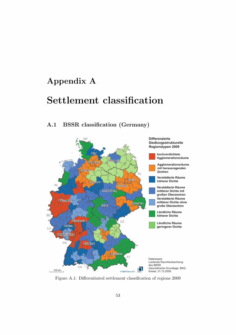
Appendix A
Settlement classification
A.1 BSSR classification (Germany)
DK
KielW
SchwerinHamburgW
BremenWPLW
BerlinWHannoverW
NLW PotsdamW
MagdeburgW
DüsseldorfWDresden
Erfurt
BEW
WiesbadenW CZWMainzW
LUW
Saarbrücken
FRW Stuttgart
MünchenWATW
CHW.33WkmW
©WBBSR Bonn 2011
DifferenzierteVSiedlungsstrukturelleVRegionstypenV2009V
hochverdichteteVAgglomerationsräumeV
AgglomerationsräumemitVherausragendenVZentrenV
VerstädterteVRäumeVhöhererVDichteV
VerstädterteVRäumeVmittlererVDichteVmitVgroßenVOberzentrenVVerstädterteVRäumeVmittlererVDichteVohneVgroßeVOberzentrenV
LändlicheVRäumeVhöhererVDichteV
LändlicheVRäumeVgeringererVDichteV
Datenbasis:WLaufendeWRaumbeobachtungWdesWBBSRWGeometrischeWGrundlage:WBKG©WKreise©W9.G.2G2339W
Figure A.1: Differentiated settlement classification of regions 2009
53

APPENDIX A. SETTLEMENT CLASSIFICATION 54
A.2 Grid characteristics [1] and [2]
The following tables show data from Scheffler’s dissertation fitted into thisprojects classification according to Table 2.2 [1].
A.2.1 Transformer characteristics
Table A.1: Typical transformer station ratings
Sr [kVA] R1 R2 U1 U2 A1 A2 A3
630 630 630 630 630 630 630400 400 400 400 400250 250 250 250160 160 160100 10050 50
Table A.2: Feeder outlets of TSts, mean and standard deviation
feeders R1 R2 U1 U2 A1 A2 A3
µ 2.2 2.8 4.6 4.4 4.3 5.0 5.8±σ 0.7 0.8 1.9 1.5 1.6 2.1 0.8
A.2.2 Load characteristics
Table A.3: Yearly electricity consumption per household, mean and standarddeviation (no confidence interval).
energy R1 R2 U1 U2 A1 A2 A3
µ [kWh] 3026 3423 3834 1853 2716 2716 1698±σ [kWh] 1078 1368 516 977 489 916 411
Table A.4: Housing units per connected building [1]
unitsbuilding R1 R2 U1 U2 A1 A2 A3
µ 1.3 1.8 1.4 8.5 9.2 5.7 41range 1–2 1–6 1–6 6–60 6–15 2–12 20–80

APPENDIX A. SETTLEMENT CLASSIFICATION 55
A.2.3 Line characteristics
Table A.5: Usage of conductor cross-section according to [2]
mm2 R U A
185 20%150 36% 84% 54%120 15%95 18% 4%70 21% 6%50 19%
other 7% 5% 12%
Table A.6: Distances between buildings’ service connections, mean and stan-dard deviation
distance R1 R2 U1 U2 A1 A2
µ [m] 48 37 16 24 31 13±σ [m] 29 17 7 8 12 7
The distances between the buildings’ service connections correspond tothe width’s of of the buildings’ lands facing public place.
A.3 Grid structure German DSO database
The DSOs database is supposed to contain the following grid characteristicsfor each voltage level and DSO: geographic and supplied area, total lengthcables, total length OHLs, installed transformer power, peak load, yearly en-ergy, grid losses, number of connected loads and inhabitants. The followingproblems arose from the database analysis:
• Supplied area (from land-use statistics) is not specified for most DSOs
• The database implied a code indicating the inclusion of service lateralsbut as the decoding was not explained the code is ignored
• the list of installed transformer power is incomplete (798 MV/LV-transformer sets but 853 LV grid sets)
• Loss information data is of insufficient quality
The following table displays the grid characteristics analyzed for the arealclasses specified in Table 2.2

APPENDIX A. SETTLEMENT CLASSIFICATION 56
∅LV
R1
R2
U1
U2
A1
A2
A3
∅M
V
sam
ple
s85
361
7271
6152
150
335
803
geo
gr.
areaA
[km
2]
506
2137
1711
863
203
481
152
81500
connec
ted
loads
CP
s625
2698
876
1242
1687
890
2342
073
023
3060
362
2592
6910
*C
Pd
ensi
ty[/
km
2]
333
4268
9512
214
721
661
32
inhab
itan
ts10
0968
1497
1021
2363
1329
5843
883
12766
956
754
9970
9101824
*pop
.den
sity
[/km
2]
570
5812
417
521
0272
389
1038
622
*in
hab
itan
ts/C
P1.
951.
761.
991.
991.
982.
072.
01
1.95
894
cable
s[k
m]
125
025
3939
1118
6668
5133
5639
817
497
OH
Ls
[km
]158
565
396
292
5140
685
40
141
*lin
es/C
P[m
]31
6336
3334
3028
233585
*lin
es/A
[km/km
2]
6.9
2.5
2.2
2.9
3.8
3.9
5.6
11.
12.6
(pea
klo
adPpk
[MW
])a
(592)
(14)
(62)
(5349)
(21)
(125)
(17)
(17)
*(Ppk/C
P[k
W])
(7.4
1)
(10.9
)(1
.6)
(2.0
)(2
.5)
(1.4
)(1
.2)
year
lyen
ergy
E[G
Wh
]27
138
157
338
611
6430
133
251
897.8
*ener
gyden
sity
[MW
h/km
2]
1802
520
313
328
589
831
952
343
314480
*ener
gyp
erC
P[k
Wh
]63
2111
974
4925
4898
5148
5599
479
2667
615.
9·1
06
pow
erin
stalled
[GV
A]
245
470
613
342
99295
121
208
*pow
er/C
P[M
VA
]4.
754.
933.
894.
254.0
33.9
53.3
2
abase
don
ver
yfe
wdata
.D
onot
use
resu
lts!
*der
ived
chara
cter
isti
cs

Appendix B
Load modeling
Table B.1: BDEW standard load profiles SLPs
SLP description
G0 general commerce (weighted average of G1-G6)G1 commerce workdays 8 a.m. to 6 p.m.G2 commerce with severe-to-predominant consumption in the eveningsG3 commerce with 24-hours consumptionG4 shops, hairdressersG5 bakeries with baking roomG6 weekend commerceL0 general farm (weighted average of L1-L2)L1 farms with dairy sectorL2 other farmsH0 general household
Table B.2: Households’ maximum power consumptions in literature
Source peak context
[36] 1.92 kW average power of maximum 15-minute energy con-sumption of a 4000 kWh household
[13] 4.5 kW 50 W/m2 and an average household size of 90 m2
[2] 30 kW based on [37] (often cited in this context)[17] 18 kW Student project. For n households per building mul-
tiply with f = n−0.52 to account for load coincidence[4] 13 kW reference benchmark grid consumer[1] 2 kW evening peak in daily power consumption diagram
(exemplary household)
57

Appendix C
Line dimensioning
Cross-section–load moment diagram and table for ∆V s [23]:C
mm2
10
16
25
35
50
70
95
120
150
185
240
300
Ku
pfe
r
1i 2i 3i 4i 5i 6i 8i 10i 20i 30i 40i 50i 60i 80i 10016240
Lastmoment P· L ·103 kW·m
1i 2i 3i 4i 5i 6i 7c
mm2
35
50
70
95
120
150
185
240
300A
lum
iniu
m
U/Uo =i400/230iVolt
cos =i0,9
Leitertemperaturi=i50°Cmm
Table C.1: Max. load moment by ∆V and aluminum cross-section
max load moment [kW m] by voltage drop ∆U
cross-section 7% 6% 5% 4% 3% 2% 1%
35 mm2 10028 8475 7206 5704 4324 2821 141650 mm2 13420 11393 9643 7645 5796 3792 190970 mm2 18947 16085 13655 10842 8224 5362 272495 mm2 25394 21655 18302 14552 11066 7207 3623
120 mm2 30946 26350 22303 17787 13505 8757 4435150 mm2 36552 30985 26227 20916 15904 10359 5200185 mm2 43951 37591 31724 25337 19266 12586 6290240 mm2 52927 45066 38089 30512 23098 15112 7563300 mm2 63076 54029 45029 36417 27691 18090 9026
58

Appendix D
Software module
D.1 Parameters
Table D.1: Constant values loaded via fixed parameters.m
name table description
R1. . . A3 2.2 population classes and densitiesE h 2.3 yearly class specific household consumption [kWh]
hh cp 2.3 household variation by classt o A.2 average number of transformer outlets by class
l cross C.1 cross-section specific load moment limits [kW m]Cmap 2.2 discrete colormap based on classification
Table D.2: Default values of parameters loaded via user parameters.m
name default description
res 100 resolution of both x and y coordinatesP pk 18 Average peak load of a single household [kW]
PpHH 2.02 Average people per householdg coinc 0.06 coincidence factor
lam 0.9 power factorCP Max 500 Maximum number of connection points per TStdistance eucl. calculation method for the distance matrixd max 0.7 maximum direct distance of CP from the TSt [km]l SgSg 2 maximum interconnections to other sub-grids
T rg max 64 maximum number of TSt connected to one MV ringdU LV 3 maximum voltage loss along LV linesdU MV 3 maximum voltage loss along MV lines
59

APPENDIX D. SOFTWARE MODULE 60
D.2 GUI handling of data
Table D.3: Descriptions of the Guide handles.-elements used in the module
elements containing figure-handles
Main Gui Main GUIMap axes plot areadatatable table below the plot areamenu show (Menu bar→)Show -Menumenu project (Menu bar→)Project-Menuuitoolbar1 Toolbar modulegrid MV (Menu bar→Show→) MV Grid -Optiongrid LV (Menu bar→Show→) LV Grid -OptionCP MV (Menu bar→Show→) MV Loads-OptionCP LV (Menu bar→Show→) LV Loads-Optionshow heatmap (Menu bar→Show→) Heatmap-Optionshow centers (Menu bar→Show→) Pop Centers-OptionOpen (Menu bar→Project→)Open Project (only callback used)Save (Menu bar→Project→) Save ProjectNew (Menu bar→Project→) New Projecttoolbar showgrid (Toolbar→)Show Grid -Buttonlegend (Toolbar→)Show Legend -Buttoncolorbar (Toolbar→)Insert Colorbar -Buttondatacursor (Toolbar→)Data Cursor -Buttonzoomin (Toolbar→)Zoom in-Buttonzoomout (Toolbar→)Zoom out-Buttonpan (Toolbar→)Pan-ButtonSaveTbar (Toolbar→)Save Project-Buttonelements containing data
output Default: Address of the main GUILV L Cell array: LV lines matrices (output 2)LV CP Cell array: LV CPs matrices (output 1)MV L Cell array: MV lines matrices (output 4)MV CP Cell array: MV CPs matrices (output 3)centers Matrix: type and position of population centersLV LD Cell array: LV loads (for plotting)LV Lc Cell array: closed LV lines (for plotting)LV Lo Cell array: open LV lines (for plotting)MV LD Cell array: MV loads(TSts) (for plotting)MV Lc Cell array: closed MV lines (for plotting)MV Lo Cell array: open LV lines (for plotting)legend data Matrix: data from the table (output 5)

APPENDIX D. SOFTWARE MODULE 61
D.3 Grid building procedure
Exemplary construction of a distribution grid in the size of the GermanLandkreis with an area of approximately 1000 km2 and 127000 Inhabitantsliving in 25 municipalities.
Figure D.1: Initialization of a new project. Input of size and inhabitantsof the supplied area.
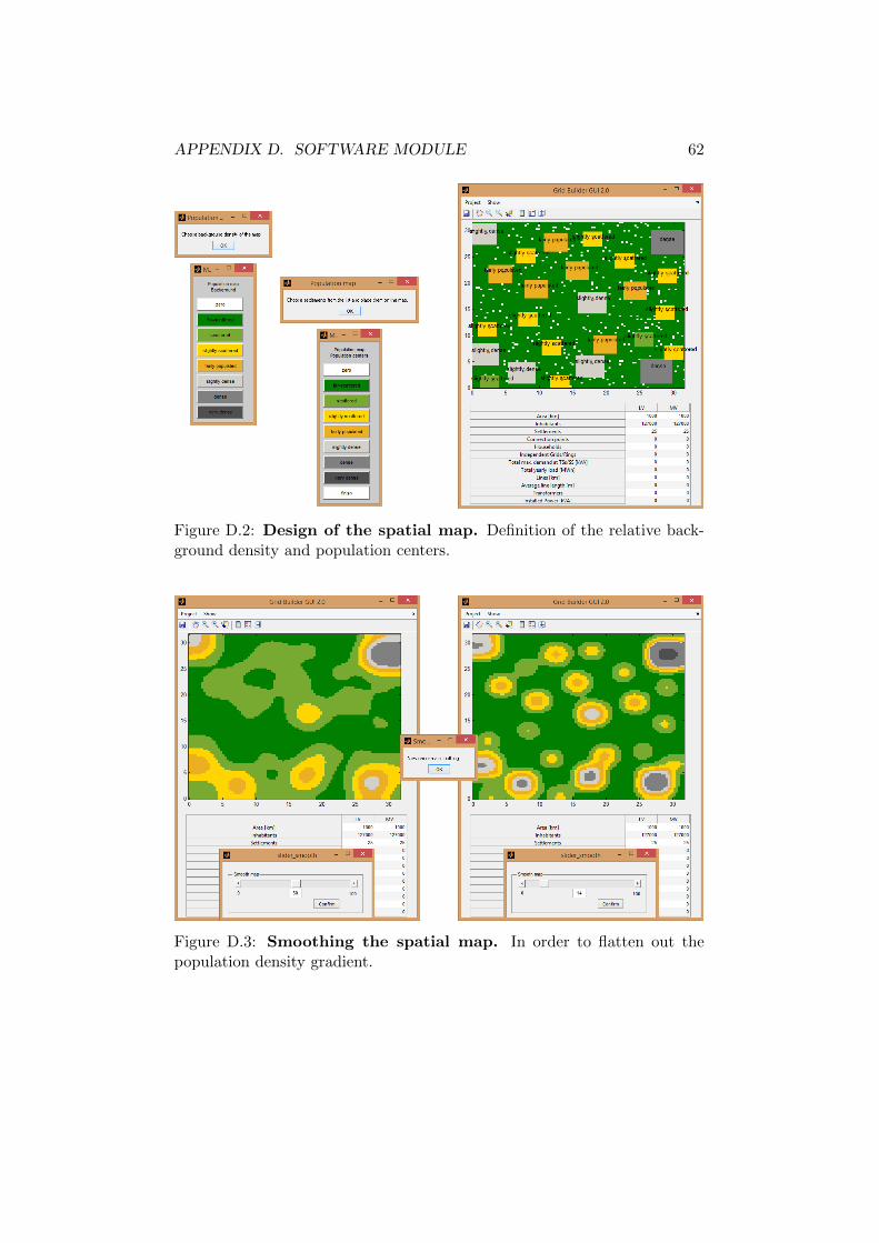
APPENDIX D. SOFTWARE MODULE 62
Figure D.2: Design of the spatial map. Definition of the relative back-ground density and population centers.
Figure D.3: Smoothing the spatial map. In order to flatten out thepopulation density gradient.

APPENDIX D. SOFTWARE MODULE 63
Figure D.4: Amount of independent LV grids. After calculation of theLV loads the number of independent grids is user-set.
Figure D.5: LV grid design options. For the dimensioning of transformersand lines the user sets three different options.
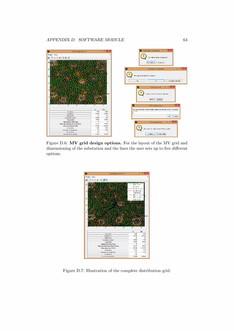
APPENDIX D. SOFTWARE MODULE 64
Figure D.6: MV grid design options. For the layout of the MV grid anddimensioning of the substation and the lines the user sets up to five differentoptions.
Figure D.7: Illustration of the complete distribution grid.

Bibliography
[1] J. Scheffler, Bestimmung der maximal zulassigen Netzanschlussleistungphotovoltaischer Energiewandlungsanlagen in Wohnsiedlungsgebieten.PhD thesis, Technische Universitat Dresden, 2002.
[2] G. Kerber, Aufnahmefahigkeit von Niederspannungsverteilnetzen fur dieEinspeisung aus Photovoltaikkleinanlagen. PhD thesis, Technische Uni-versitat Munchen, 2011.
[3] S. Koch, A. Ulbig, and F. Ferrucci, “An innovative software platformfor simulation and optimization of active distribution grids for DSOSand smartgrid researchers,” in CIRED Workshop 2014, 2014.
[4] S. Papathanassiou, N. Hatziargyriou, and K. Strunz, “A benchmarklow voltage micgrogrid network,” in CIGRE Symposium - Power sys-tems with dispersed generation: technologies, impacts on development,operation and performances, 2005.
[5] W. Kersting, “A comprehensive distribution test feeder,” in Transmissi-on and Distribution Conference and Exposition, 2010 IEEE PES, pp. 1–4, April 2010.
[6] K. Rudion, A. Orths, Z. A. Styczynski, and K. Strunz, “Design ofBenchmark of Medium Voltage Distribution Network for Investigati-on of DG Integration,” in Power Engineering Society General Meeting,IEEE, 2006.
[7] H. Rui, A. M., and W. Wellssow, “Synthetic Medium Voltage Grids forthe Assessment of Smart Grid Techniques,” in 3rd IEEE PES InnovativeSmart Grid Technologies Europe (ISGT Europe), Berlin, 2012.
[8] P. Schulz, J. Heitzig, and K. Jurgen,“A random growth model for powergrids and other spatially embedded infrastructure networks,”Eur. Phys.J. Special Topics, vol. 223, pp. 2593–2610, 2014.
[9] “Verordnung uber den Zugang zu Elektrizitatsversorgungsnetzen(StromNZV) §17.”
65

BIBLIOGRAPHY 66
[10] “Verordnung uber die Entgelte fur den Zugang zu Elektrizitatsversor-gungsnetzen (StromNEV) §27.”
[11] A. A. Sallam and O. P. Malik, Electric Distribution System. IEEE PressSeries on Power Engineering, Wiley, 2011.
[12] J. Schlabbach and K.-H. Rofalski, Power System Engineering, PlanningDesing and Operation of Power Systems and Equipment. Wiley-VCH,2014.
[13] G. Lipphardt, Elektrische Anlagen und Netze. Hochschule Mannheim,2006.
[14] H. Janich, “Laufende Raumbeobachtung - Raumabgrenzungen, Sied-lungsstrukturelle Regionstypen.” Online, 2011.
[15] A. J. Schwab, Elektroenergiesysteme : Erzeugung, Transport, Ubertra-gung und Verteilung elektrischer Energie. Springer Berlin, 2. ed., 2012.
[16] W. H. Kersting, Distribution System Modeling and Analysis. ElectricPower Engineering, CRC Press, 2002.
[17] P. Forjan, G. Schriebl, and W. C. Schuster, “Energieverteilung in Hoch-, Mittel- und Niederspannungsnetzen,” Master’s thesis, HTBL u. VABULME Graz-Gosting, 2006.
[18] “Three-phase oil-immersed distribution transformers 50 hz, from 50 kvato 2500 kva with highest voltage for equipment not exceeding 36 kv -part 1: General requirements; german version en 50464-1:2007.”
[19] “Iec 60076-7:2005 power transformers - part 7: Loading guide for oil-immersed power transformers.”
[20] H. Kiank and W. Fruth, Planning Guide for Power Distribution Plants:Design, Implementation and Operation of Industrial Networks. PublicisPublishing, 2011.
[21] U. Post, “Grundlagen der Energietechnik: Netze und Betriebsmittel -Netzformen.” Online, Coursescript, September 2007.
[22] T. Haase and H. Weber, “Optimierung von Mittelspannungsnetzenregionaler Energieversorger,” in 10.Symposium Maritime Elektronik,pp. 147–150, Arbeitskreis Energie- und Steuerungstechnik, 2001.
[23] Infrastruktur Kabelsysteme, “Auslegung Kabelsysteme,” tech. rep.,Brugg Cables, 2014.
[24] “En 50160:2011-02, voltage characteristics of electricity supplied by pu-blic distribution networks; german version en 50160:2010.”

BIBLIOGRAPHY 67
[25] J. Nesetril and H. Nesetrilova, “The Origins of Minimal Spanning TreeAlgorithms – Boruvka and Jarnık,”Documenta Mathematica, vol. ExtraVolume ISMP, pp. 127–141, 2012.
[26] Y. Backlund and J. Bubenko, “Distribution System Design Using Com-puter Graphics Technique,” in Power Industry Computer ApplicationsConference, 1979. PICA-79. IEEE Conference Proceedings, pp. 382–388, May 1979.
[27] R. Prim, “Shortest Connection Networks And Some Generalizations,”The Bell System Technical Journal, vol. 36, pp. 1389–1401, 1957.
[28] A. K. Jain, M. N. Murty, and P. J. Flynn, “Data clustering: A review,”ACM Comput. Surv., vol. 31, pp. 264–323, Sept. 1999.
[29] Z. Bozic and E. Hobson, “Urban underground network expansion plan-ning,” Generation, Transmission and Distribution, IEE Proceedings-,vol. 144, pp. 118–124, Mar 1997.
[30] G. Reeves, “smooth2a.m.” Matlab File Exchange, March 2009.
[31] P. Wied, “heatmap.js.” Online, October 2014.
[32] T. Okraszewski, G. Balzer, and C. Schorn,“Restructuring of the existingmedium voltage cable networks using segmentation method - Impacton networks reliability,” in CIRED, 19th International Conference onElectricity Distribution, 2007.
[33] D. S. Johnson and L. A. McGeoch, “The traveling salesman problem:A case study in local optimization,” Local search in combinatorial opti-mization, vol. 1, pp. 215–310, 1997.
[34] A. Kovacs, “Solving the Vehicle Routing Problem with Genetic Algo-rithm and Simulated Annealing,” Master’s thesis, Hogskolan Dalarna,Sweden, May 2008.
[35] T. C. M. Caldeira, “Optimization of the Multi-Depot Vehicle RoutingProblem: an Application to Logistics and Transport of Biomass forElectricity Production,” Master’s thesis, Universidade Tecnica da Lis-boa, October 2009.
[36] BDEW, “Lastprofilverfahren Strom.” Excel-Sheet, December 2014.
[37] W. Kaufmann, Planung offentlicher Elektrizitatsverteilungssysteme.VDE, 1995.