
Topological string theory from D-brane bound states - Harvard
234
Topological string theory from D-brane bound states A dissertation presented by Daniel Louis Jafferis to The Department of Physics in partial fulfillment of the requirements for the degree of Doctor of Philosophy in the subject of Physics Harvard University Cambridge, Massachusetts June 2007
Transcript of Topological string theory from D-brane bound states - Harvard

Topological string theory from D-brane boundstates
A dissertation presented
by
Daniel Louis Jafferis
to
The Department of Physics
in partial fulfillment of the requirements
for the degree of
Doctor of Philosophy
in the subject of
Physics
Harvard University
Cambridge, Massachusetts
June 2007

c©2007 - Daniel Louis Jafferis
All rights reserved.

Thesis advisor Author
Cumrun Vafa Daniel Louis Jafferis
Topological string theory from D-brane bound states
Abstract
We investigate several examples of BPS bound states of branes and their associated
topological field theories, providing a window on the nonperturbative behavior of the
topological string.
First, we demonstrate the existence of a large N phase transition with respect to
the ’t Hooft coupling in q-deformed Yang-Mills theory on S2. The Ooguri-Strominger-
Vafa [62] relation of this theory to topological strings on a local Calabi-Yau [7],
motivates us to investigate the phase structure of the trivial chiral block at small
Kahler moduli. Second, we develop means of computing exact degeneracies of BPS
black holes on certain toric Calabi-Yau manifolds. We show that the gauge theory on
the D4 branes wrapping ample divisors reduces to 2D q-deformed Yang-Mills theory
on necklaces of P1’s. At large N the D-brane partition function factorizes as a sum
over squares of chiral blocks, the leading one of which is the topological closed string
amplitude on the Calabi-Yau, in agreement with the conjecture of [62].
Third, we complete the analysis of the index of BPS bound states of D4, D2 and
D0 branes in IIA theory compactified on toric Calabi Yau, demonstrating that they
are encoded in the combinatoric counting of restricted three dimensional partitions.
We obtain a geometric realization of the torus invariant configurations as a crystal
iii

Abstract iv
associated to the bound states of 0-branes at the singular points of a single D4 brane
wrapping a high degree equivariant surface that carries the total D4 charge. The
crystal picture provides a direct realization of the OSV relation to the square of the
topological string partition function, which in toric Calabi Yau is also equivalent to a
theory of three dimensional partitions. Finally, we apply the techniques of the quiver
representation of the derived category of coherent sheaves to discover a topological
matrix model for the index of BPS states of D2 and D0 branes bound to a 6-brane.
This enables us to examine the quantum foam [37] description of the A-model by
embedding it in the full string theory.

Contents
Title Page . . . . . . . . . . . . . . . . . . . . . . . . . . . . . . . . . . . . iAbstract . . . . . . . . . . . . . . . . . . . . . . . . . . . . . . . . . . . . . iiiTable of Contents . . . . . . . . . . . . . . . . . . . . . . . . . . . . . . . . vCitations to Previously Published Work . . . . . . . . . . . . . . . . . . . viiiAcknowledgments . . . . . . . . . . . . . . . . . . . . . . . . . . . . . . . . ix
1 Introduction and Summary 1
2 Phase Transitions in q-Deformed Yang-Mills and Topological Strings 152.1 Introduction . . . . . . . . . . . . . . . . . . . . . . . . . . . . . . . . 152.2 The Douglas-Kazakov Phase Transition in Pure 2-D Yang-Mills theory 22
2.2.1 Review of the Exact Solution . . . . . . . . . . . . . . . . . . 222.2.2 The Phase Transition at θ = 0 . . . . . . . . . . . . . . . . . . 252.2.3 Instanton Sectors and θ 6= 0 . . . . . . . . . . . . . . . . . . . 28
2.3 The q-deformed Theory . . . . . . . . . . . . . . . . . . . . . . . . . . 332.3.1 Review of the Exact Solution . . . . . . . . . . . . . . . . . . 332.3.2 The Phase Transition at θ = 0 . . . . . . . . . . . . . . . . . . 362.3.3 Instanton Sectors and θ 6= 0 . . . . . . . . . . . . . . . . . . . 39
2.4 Chiral decomposition, and phase transition in topological string . . . 442.4.1 Interpretation of the trivial chiral block . . . . . . . . . . . . . 462.4.2 Phase Structure of the Trivial Chiral Block . . . . . . . . . . . 48
2.5 Concluding Remarks . . . . . . . . . . . . . . . . . . . . . . . . . . . 54
3 Branes, Black Holes and Topological Strings on Toric Calabi-Yau 613.1 Introduction . . . . . . . . . . . . . . . . . . . . . . . . . . . . . . . . 613.2 Black holes on Calabi-Yau manifolds . . . . . . . . . . . . . . . . . . 64
3.2.1 D-brane theory . . . . . . . . . . . . . . . . . . . . . . . . . . 643.2.2 Gravity theory . . . . . . . . . . . . . . . . . . . . . . . . . . 653.2.3 D-branes for large black holes . . . . . . . . . . . . . . . . . . 663.2.4 An Example . . . . . . . . . . . . . . . . . . . . . . . . . . . . 68
3.3 The D-brane partition function . . . . . . . . . . . . . . . . . . . . . 71
v

Contents vi
3.3.1 Intersecting D4 branes . . . . . . . . . . . . . . . . . . . . . . 743.3.2 Partition functions of qYM . . . . . . . . . . . . . . . . . . . . 763.3.3 Modular transformations . . . . . . . . . . . . . . . . . . . . . 80
3.4 Branes and black holes on local P2. . . . . . . . . . . . . . . . . . . 823.4.1 Black holes from local P2 . . . . . . . . . . . . . . . . . . . . 843.4.2 Branes on local P2 . . . . . . . . . . . . . . . . . . . . . . . . 91
3.5 Branes and black holes on local P1 ×P1 . . . . . . . . . . . . . . . . 973.5.1 Black holes on local P1 ×P1. . . . . . . . . . . . . . . . . . . 993.5.2 Branes on local P1 ×P1 . . . . . . . . . . . . . . . . . . . . . 103
3.6 Branes and black holes on Ak ALE space . . . . . . . . . . . . . . . . 1053.6.1 Modularity . . . . . . . . . . . . . . . . . . . . . . . . . . . . 1093.6.2 The large N limit . . . . . . . . . . . . . . . . . . . . . . . . . 111
4 Crystals and intersecting branes 1244.1 Introduction . . . . . . . . . . . . . . . . . . . . . . . . . . . . . . . . 1244.2 BPS bound states of the D4/D2/D0 system . . . . . . . . . . . . . . 129
4.2.1 Turning on a mass deformation for the adjoints . . . . . . . . 1344.3 Localization in the Higgs branch of the theory of intersecting branes . 136
4.3.1 Solving the twisted N = 4 Yang Mills theory . . . . . . . . . . 1384.4 Propagators and gluing rules . . . . . . . . . . . . . . . . . . . . . . . 1424.5 The crystal partition function . . . . . . . . . . . . . . . . . . . . . . 146
4.5.1 One stack of N D4 branes . . . . . . . . . . . . . . . . . . . . 1484.5.2 N D4 branes intersecting M D4 branes . . . . . . . . . . . . . 1514.5.3 The general vertex . . . . . . . . . . . . . . . . . . . . . . . . 154
4.6 Chiral factorization and conjugation involution . . . . . . . . . . . . . 1574.7 Concluding remarks and further directions . . . . . . . . . . . . . . . 160
5 Quantum foam from topological quiver matrix models 1645.1 Introduction . . . . . . . . . . . . . . . . . . . . . . . . . . . . . . . . 1645.2 Review of quivers and topological matrix models . . . . . . . . . . . . 171
5.2.1 A quiver description of the classical D6-D0 moduli space . . . 1715.2.2 Quiver matrix model of D0 branes . . . . . . . . . . . . . . . . 173
5.3 Solving the matrix model for D6/D0 in the vertex . . . . . . . . . . . 1805.3.1 Computing the Euler character of the classical moduli space . 1845.3.2 Generalization to the U(M) Donaldson-Thomas theory . . . . 188
5.4 The full vertex Cµνη . . . . . . . . . . . . . . . . . . . . . . . . . . . . 1895.4.1 One nontrivial asymptotic of bound D2 branes . . . . . . . . . 1905.4.2 Multiple asymptotics and a puzzle . . . . . . . . . . . . . . . . 199
5.5 Effective geometry, blowups, and marginal stability . . . . . . . . . . 2045.5.1 Probing the effective geometry of a single 2-brane with N 0-branes2105.5.2 Example 2: the geometry of C¤¤· . . . . . . . . . . . . . . . . 2135.5.3 An example with three 2-branes . . . . . . . . . . . . . . . . . 215

Contents vii
5.6 Conclusions and further directions . . . . . . . . . . . . . . . . . . . . 217
Bibliography 220

Citations to Previously Published Work
The arguments given in Chapter 2 were obtained in collaboration with Joseph Marsano.The text has appeared previously in
D. Jafferis and J. Marsano. “A DK phase transition in q-deformed Yang-Mills on S2 and topological strings,” arXiv:hep-th/0509004.
I also want to acknowledge M. Marino, S. Minwalla, L. Motl, A. Neitzke, K. Pa-padodimas, N. Saulina, and C. Vafa for valuable discussions related to the materialin this chapter.
The results of Chapter 3 were obtained in collaboration with Mina Aganagic andNatalia Saulina. The text has appeared previously in
‘M. Aganagic, D. Jafferis and N. Saulina. “Branes, black holes and topo-logical strings on toric Calabi-Yau manifolds,” JHEP 0612, 018 (2006)[arXiv:hep-th/0512245].
I also want to acknowledge F. Denef, J. McGreevy, M. Marino, A. Neitzke, T. Okuda,and H. Ooguri for valuable discussions related to the material in this chapter, andespecially C. Vafa for collaboration on a related project.
The text of Chapter 4 has appeared previously in
D. Jafferis. “Crystals and intersecting branes,” arXiv:hep-th/0607032.
I also want to acknowledge Mina Agaganic, Joe Marsano, Natalia Saulina, CumrunVafa, and Xi Yin for valuable discussions related to the material in this chapter.
Finally, the text of Chapter 5 has appeared previously in
D. Jafferis. “Quiver matrix models and quantum foam”, arXiv:0705.2250
I also want to acknowledge Emanuel Diaconescu, Davide Giaotto, Greg Moore, LubosMotl, Natalia Saulina, Alessandro Tomasiello, and Xi Yin for valuable discussionsrelated to the material in this chapter, and especially Robbert Dijkgraaf and CumrunVafa for collaboration on a related project.
viii

Acknowledgments
I want to thank first my advisor, Cumrun Vafa, for his guidance and the many
insightful discussions we had. It has been a privilege to work with him, and a pleasure
to learn from the depth and clarity of his vision of topological string theory. The third
and fifth chapters of this thesis are based on work that initially developed out of some
of his suggestions.
It goes without saying that I extent my gratitude to my collaborators, Mina
Aganagic, Joe Marsano, and Natalia Saulina, who co-authored the papers that are
essentially reproduced as the second and third chapters. I have gained immeasurably
from the time we spent fruitfully thinking together.
One of the reasons why my experience at Harvard was all I could have ever hoped
it would be was the lively and stimulating atmosphere of the string theory group. It
was always pleasure to speak of physics and life with the theoretical physics faculty,
particularly Andy Strominger, Shiraz Minwalla, Arthur Jaffe, and Lubos Motl. Many
of my best ideas were clarified in interesting discussions with the string theory post-
docs; besides my collaborators, I particularly want to thank Sergei Gukov, Marcos
Marino, and Davide Gaiotto for sharing their astute perspectives. My life at Harvard
was made far smoother by the efficiency and kindness of the department administra-
tors Nancy Partridge and Sheila Ferguson, who helped arrange everything from the
logistics of funding to the mailing of letters of recommendation.
Some of my fondest memories will be of fine dinners and stimulating conversations
about physics with my fellow graduate students. I particularly want to thank Xi Yin,
Andy Neitzke, Greg Jones, Joe Marsano, Kirill Saraikin, Monica Guica, Lisa Huang,
Aaron Simons, Itay Yavin, and Martijn Wijnholt for many interesting discussions.
ix

Acknowledgments x
My wonderful friends - Svetlana, Greg, Ali, Oleg, Gordon, Xi, Monica, and others
too numerous to name - have made my life at Harvard always enjoyable, steeped with
urbane wit and congenial conversation.
Finally, I thank my parents, Dorene and Jim, and my brother, Noah, for their
loving support, and for always being there for me whenever I needed them.

Chapter 1
Introduction and Summary
One of the most effective windows on the theory of quantum gravity is the search
for the microscopic origin of the entropy of black holes that is predicted from low
energy field theory and thermodynamics. The matching of the microscopic statistics
of D-brane bound states with the supergravity entropy of 1/4 the area of the event
horizon by Strominger and Vafa has been referred to as the most important calculation
in string theory.
A particularly rich extension of this original computation is to the case of black
holes in N = 2 four dimensional compactifications of type II strings on a Calabi Yau
3-fold which preserve half of the supersymmetries. The protection of the relevant
indexed entropies from perturbative and nonperturbative gs corrections, which allows
one to directly identify the states of the weakly coupled worldvolume theory living on
certain D-branes with those of the semiclassical black hole at strong coupling, appears
to depend crucially on supersymmetry (although see [63] for a possible generalization).
The case of half BPS objects in N = 2 supergravity in four dimensions provides the
1

Chapter 1: Introduction and Summary 2
most diverse and fascinating environment in which exact calculations have been done
to date.
Almost as a side effect, this has led to deep mathematical insights in algebraic
geometry, enumerative geometry and topological string theory. The curvature of the
branes’ worldvolume, wrapping cycles in the Calabi-Yau manifold, causes their world-
volume gauge theories to become twisted [14]. This twisting of the supersymmetries
renders the resulting theories topological in the internal manifold. In this work, we
will explore some of the wonderful relations among topological invariants that have
been discovered via their embedding into string theory.
The fact that the dilaton lies in the universal hypermultiplet, together with a
theorem that vectors and hypers cannot mix in N = 2 supersymmetric theories,
implies that BPS quantities involving the vector multiplets and thus Kahler geometry
in IIA will be string tree level exact, to all orders in perturbation theory and even
non-perturbatively. The Kahler structure of the moduli spaces of BPS branes can
receive α′ corrections, but index is also protected from these corrections that would
depend on the background Kahler moduli away from walls in Calabi-Yau moduli
space where it can jump.
On the other hand, the vector multiplets can gravitate. Hence one expects cor-
rections to the classical geometry of moduli space when fields in the four dimensional
gravity multiplet are turned on. Those which can influence BPS quantities turn out
to have a particularly elegant form, coming from F-terms in the effective action,
∫d4xFg(X
I)(R2+F 2g−2
+ ),
where R+ and F+ are the self-dual components of the Ricci tensor and graviphoton

Chapter 1: Introduction and Summary 3
field strength, and XI represent the geometric vector multiplets. This term aries at
genus g, although no powers of the string coupling enter due to the magic of string
perturbation theory, and the crucial function Fg is exactly the genus g topological
string amplitude. Therefore the coupling of the topological string theory is naturally
identified with the background field strength, F+. Starting with the work of [62],
it has become possible compare microscopic and supergravity calculations of these
subleading corrections to the classical entropy to all orders in perturbation theory.
Their remarkable conjecture, which has been verified in numerous papers (see [35]
for a list of references), is that the perturbative corrections to the indexed entropy of
BPS black holes, in a mixed ensemble for the electric and magnetic brane charges,
are exactly twice the real part of the topological string prepotential evaluated at the
attractor values of the Calabi-Yau moduli. Hence the index of BPS states, which is
obviously integral, can be expressed in the large charge limit as a formal Legendre
transformation of the square of a holomorphic object, namely the topological string
partition function.
The topological string behaves as a wavefunction in the quantization of the classi-
cal phase space of vector moduli, as was first derived from the holomorphic anomaly
equations [13] [71]. In the near horizon limit of the BPS black holes we will be
discussing, it appears to be related to quantization in the radial direction. A more
complete understanding of the quantum evolution in this emergent dimension in the
context of AdS/CFT might provide powerful new insights into the long standing prob-
lem of emergent time in string theory. The OSV relation provides a partial window
into these ideas in an elegant and computable BPS regime of string theory, giving a

Chapter 1: Introduction and Summary 4
tantalizing hint of the way the index of microstates, in the ordinary sense, is captured
by the Wigner density associated to the wavefunction of a kind of radial quantization.
One of the main themes of this thesis is the search for a non-perturbative comple-
tion of topological string theory. The A-model partition function expressed in terms
of the Gromov-Witten invariants as
Ftop =∑g≥0
∑nA≥0∈H2
Fg nAg2g−2
top e−n· t, (1.1)
is a perturbative expression both in the topological string coupling and about the
large volume limit. Mirror symmetry relates this theory to the B-model, which can
naturally be expanded about any basepoint in the moduli space of complex structures.
The dependence of the partition function on the basepoint is expressed genus by genus
in terms of the holomorphic anomaly equations.
By studying the B-model near singular points in the moduli of complex structures,
corresponding to the formation of a conifold in the Calabi-Yau geometry, one can
relate the genus amplitudes in an appropriate scaling limit to the perturbation series
of the c = 1 string. This is known to be an asymptotic expansion, and moreover is
not Borel resummable. Hence new objects must rescue the theory if it is to have a
sensible non-perturbative completion.
Because the topological string computes corrections to the F-terms of the super-
string, it is natural to assume that its non-perturbative completion is related to BPS
objects in II theory compactified on a Calabi-Yau. In the following chapters, we will
explore several distinct but interconnected ways of embedding the topological string
in theories of BPS branes. The integer invariants constructed from these bound states
shed light on the beautiful integral structures which emerge from topological string

Chapter 1: Introduction and Summary 5
theory.
This thesis will be primarily focused on the description of BPS bound states
of branes in type II string theory compactified on Calabi-Yau manifolds, and their
relation to topological string theory. I will investigate both the qualitative aspects of
these systems, including their phase structure on certain local Calabi-Yau manifolds,
as well as their beautiful mathematics of modular forms, derived category of coherent
sheaves, crystal partition functions, and asymptotic factorization. Much of this work
has centered on various techniques of analyzing topological gauge theories in different
dimensions, ranging from the physical methods utilizing the structure of the Higgs
branch of the mass deformed theory, mathematical methods of counting equivariant
sheaves, the quiver description of the derived category, and a geometric realization as
branes wrapping toric nonreduced subschemes.
The worldvolume theory of D4 branes with fluxes carrying D2 and D0 charge in IIA
theory compactified on a Calabi-Yau, X, has a whole web of dual descriptions that can
naturally be thought of as expansions about particular regimes of the moduli space of
the branes. The full quantum theory should explore the entire classical BPS moduli
space, and the exact relations between the web of theories encoding these dynamics
has yet to be completely elucidated. When the 4-branes are wrap very ample cycles
with sufficient deformations in the Calabi-Yau, the most natural description at generic
points in their moduli space is the MSW CFT obtained by lifting to M-theory. This
theory encodes the effective dynamics of M5 branes wrapping a surface in X, and
lives on the remaining T 2 of the M5 worldvolume. However, the exact theory is not
yet known in any example.

Chapter 1: Introduction and Summary 6
The opposite limit is the branch of moduli space when the D4 branes become
coincident, and are naturally thought of in terms of the U(N) Vafa-Witten theory.
Calculations here are much more doable, and in principle reproduce the complete
answer when the compactification of the adjoint scalars is properly taken into account.
In addition, branes wrapping rigid cycle can also be analyzed, although this has proved
calculationally difficult in practise, often requiring one to resort to mathematical
classifications of bundles, such as the work of [43] on equivariant P2. Moreover,
because of the topological nature of the supersymmetric partition function, much of
the index can be thought of as arising from the singularities in the classical D4 BPS
moduli space, which is exactly when the enhancement to U(N) occurs. Intermediate
between these two limits is the crystal picture explained in the fourth chapter, where
the limiting singular geometry of the wrapped surface is examined directly.
Tuning the moduli of the Calabi-Yau to the Gepner point mixes branes of various
dimension, and leads to their description in terms of a quiver theory. The derived
category of coherent sheaves, which is the mathematical object given by the moduli
space of BPS bound states of D-branes in IIA theory, has a simplified representation
in terms of fractional branes at this special point in the Kahler moduli space. We
extrapolate the matrix models found here to the opposite, large volume, limit in
the fifth chapter, finding a striking agreement with the worldvolume gauge theories
typically used there. Moreover, these quiver theories can also be interpreted as the
collective coordinates of the moduli space of instantons in the worldvolume theory of
Donaldson-Thomas for 6-branes, and Vafa-Witten for 4-branes.
The D4 brane U(N) gauge theory on a very ample divisor reduces to a theory on

Chapter 1: Introduction and Summary 7
the canonical curve [70] [44] that is further highly constrained by modular invariance.
In special cases when the Calabi-Yau has toric symmetries (including the S1 symmetry
of the fiber of local Calabi-Yau) there exist a significantly different two dimensional
reduction to q-deformed Yang-Mills theory. The relation between these two ideas is
not fully understand, and which description is more useful depends on the question.
The canonical curve approach is the natural way to understand the modular invariance
of the four dimensional Vafa-Witten theory , while q-deformed Yang-Mills provides a
window into the large charge OSV factorization.
One amazing feature of this plethora of descriptions of the BPS sector of D-branes
on a Calabi-Yau is that they all depend on the background Kahler moduli, rather
than the attractor values. This is perhaps less surprising because of the topological
nature of the index of BPS states, which is therefore locally independent of these
asymptotic moduli. But incredibly these microscopic descriptions, which seem to
naively live only inside the black hole horizon, are able to encode all the information
about different attractor tree flows and multi-centered solutions.
This is particularly apparent in the fifth chapter, as we find that the topological
quiver matrix model knows quite detailed information about the pattern of attractor
flow. Perhaps most amusingly, the correct partition function can often be computed
using the worldvolume theory of some branes that exist at the asymptotic values of
the attractor moduli, but which have already decayed once we reach at the horizon!
This is analogous to the fact that large pieces of the full entropy can be calculated
even using the description valid in some small corner of the moduli space of the
branes, as we see in many examples in the third and fourth chapters.

Chapter 1: Introduction and Summary 8
One of my primary motivations in this research has been to confirm, explore, and
refine the OSV relation of the index of BPS bound states arising in four dimensional
black holes in a mixed ensemble, to the square of the topological string wavefunction
at the attractor values of the moduli. Of particular interest is the subtle interplay
between the OSV relation and the AdS/CFT correspondence, which could shed fur-
ther light on both. If the topological quiver models introduced in the fifth chapter
become amenable to large N matrix models techniques, then there may be a sense in
which they provide a zero dimensional “CFT” dual to the topological string, which
is associated to the semi-classical Calabi-Yau geometry expected to emerge from the
appropriate limit of the matrix model.
In the second chapter, I will investigate the instanton-induced large N phase
transition with respect to the ’t Hooft coupling in q-deformed Yang-Mills theory on a
sphere. This theory is equivalent to the four dimensional topologically twisted N = 4
Yang-Mills theory that describes the BPS bound states of D4 branes wrapping the
divisor O(−p) → P1 in the local Calabi-Yau geometry O(−p)⊕O(p− 2) → P1, with
chemical potentials for D0 and D2 branes. Hence the third order phase transition we
discover is relevant to the OSV conjecture, at least in its application to noncompact
geometries. We study the phase diagram in terms of the ’t Hooft coupling and
instanton potential (θ angle), finding an intriguing interplay between the dominance
of instanton contributions and the formation of a clumped saddle point distribution.
Furthermore, this leads one to examine the related phase structure of the topological
string partition function.
The q-deformed Yang Mills in two dimensions, which is a topological theory with

Chapter 1: Introduction and Summary 9
no local degrees of freedom, can be obtained from the ordinary Yang Mills by com-
pactifying the scalar dual to the field strength in two dimensions. This modification
naturally arises in the reduction of the D4 worldvolume theory along the fiber direc-
tion, where this scalar field comes from a holonomy of the four dimensional gauge
field. The precise choice of boundary conditions at infinity in the wrapped divisor
must be those which correspond to physically having no D2 branes wrapping the
fibers.
The partition function of this theory on a genus g Riemann surface can be solved
exactly by doing the Gaussian integrals in the path integral, or by cutting and gluing
rules, with the result
Z =∑
R−U(N)
(dimq R)2−2g qpC2(R)/2eiθC1(R). (1.2)
Expressing this in terms of the weights of the representation R in ZN , it looks like
a matrix model with an attractive quadratic potential, competing with a repulsive
force between the eigenvalues for genus 0. As in the pure Yang Mills theory studied
by Gross-Taylor, Douglas-Kazakov, the strong coupling phase features a chiral fac-
torization into a pair of Fermi seas on opposite sides of a clump with the maximal
density imposed by integrality.
From the point of view of the D-brane theory, this corresponds to the regime where
the attractor value of the size of the P1 is sufficiently large, and the OSV conjecture
holds. The appearance of a sum over chiral blocks in the factorization into topological
string and anti-topological string results from working from not working in the mixed
ensemble for the noncompact D2 charges, but rather setting them to zero [6]. As the
’t Hooft coupling, λ = g2Y MN , is reduced, a phase transition occurs, and there is no

Chapter 1: Introduction and Summary 10
factorization when the attractor size becomes too small. This can be interpreted as
a regime in which multi-centered black hole solutions are not suppressed.
The phase transition can be further illuminated by an analysis of the instanton
which can contribute to the q-deformed Yang-Mills theory. The weak coupling phase is
characterized by a single instanton sector dominating the path integral. This method
enables one to investigate the structure of the phase diagram for nonzero θ, where
the ordinary real saddle point techniques fail.
By now, there have been numerous checks and demonstrations of the OSV relation,
which have shed further light on its meaning, and uncovered new subtleties. In the
third chapter, we confirm the large charge chiral factorization of the indexed entropy
into the square of the topological string wavefunction on various toric Calabi-Yau
manifolds with a single compact 4-cycle. In addition we make contact between the
methods used in [69] and [7] and the established calculations of [58] for topological
gauge theory on resolutions of An singularities. We extend and develop the technology
of solving Vafa-Witten theory in terms of q-deformed Yang-Mills to a much wider class
of examples, and elucidate the role of very ampleness in the OSV relation from the
perspective of the topological gauge theory on the D4 brane worldvolume.
The worldvolume theory of D4 branes wrapping ample divisors, with possible
intersections in the fiber, is shown to reduce to a series of coupled q-deformed Yang-
Mills on a necklace of P1’s. The explicit examples considered are local P2, P1×P1, and
Ak type ALE space times C. We found that in general the structure of chiral blocks
can be quite complicated, indicative of the structure of relevant noncompact moduli.
Never the less, in all cases we were able to extract the leading term, and match it to

Chapter 1: Introduction and Summary 11
the squared topological string amplitude on the Calabi-Yau at the attractor values of
the moduli.
When D4 branes intersect, there will be bifundamental matter living on the in-
tersection curve. If both wrap divisors of the form O(−p) → Σg, and intersect in the
fiber over an intersection point of the base Riemann surfaces in the Calabi-Yau, then
we show how this matter can be integrated out. The resulting q-deformed Yang-Mills
theories on the base curve are thus coupled at the intersection point by the oper-
ator insertions we found. Thus we find that these two dimensional avatars of the
intersecting Vafa-Witten theories are a useful tool in a wide range of geometries.
The modular properties of the BPS indexed partition functions were examined,
and were found to be consistent with the s-duality of the four dimensional topological
gauge theories. The exact results were often not very transparent, due to the mixing of
different boundary conditions in the noncompact divisors under the electro-magnetic
duality.
I found a beautiful connection between the statical mechanics of melting crystals
in a truncated room and the torus invariant bound states of D4/D2/D0 branes in a
large class of toric Calabi-Yau geometries, which is described in the fourth chapter.
This involves the careful study of ideal sheaves on a nonreduced subscheme that
makes its appearance in the “nilpotent Higgs branch” of the D4 brane moduli space,
and the use of a transfer matrix approach to counting three dimensional partitions.
In addition to providing an exciting new geometric realization of certain instanton
configurations, this enables us to find an exceptionally elegant realization of the OSV
factorization in terms of the asymptotically related topological string crystals.

Chapter 1: Introduction and Summary 12
The chiral limit of the 4-brane theory is obtained at large N by forgetting about
the truncation, which immediately results in the correct crystal description of the
topological string amplitude at the attractor value of the moduli. The anti-chiral block
can be found by utilizing the a priori surprising invariance of the crystal partition
function under conjugation of the representations along the toric legs. Subleading
chiral blocks appear because of nontrivial configurations connecting the chiral and
anti-chiral regions with order N boxes, which survive in the ’t Hooft limit.
In this way, the curious relationship between three dimensional partitions of height
less than N and unknot invariants of U(N) Chern-Simons theory found in [61] is ex-
plained. The link invariants are ubiquitous, and the crystal is secretly a calculation
involving 4-branes, rather than Donaldson-Thomas theory. Further connections be-
tween these points of view remain to be explored.
These crystals are a totally new method of counting the Euler character of the
moduli space of equivariant instantons of the U(N) Vafa-Witten theory. The three
dimensional partitions we find literally correspond to the T 3 invariant BPS bound
states, and are able to automatically encode the effect of topological bifundamental
matter living on the intersections of D4 branes. One should think of the crystal theory
as intermediate between the U(N) Vafa-Witten theory which is a good description
of the corner of moduli space where the D4 branes are coincident, and the MSW
conformal field theory [49], which is suited to the generic branch of the moduli space
when the D4 charge is carried by a smooth high degree surface in the Calabi-Yau.
It is natural to conjecture that even for non-toric Calabi-Yau, X, the partition
function of twisted N = 4 U(N) Yang-Mills on a surface, S, is equivalent to the

Chapter 1: Introduction and Summary 13
generating function of the Euler characters of the moduli spaces of ideal sheaves on
a “thickened” subscheme, S ⊂ X. This is the carefully defined version of the U(1)
theory living on the nonreduced subscheme which is the singular coincident limit of
a smooth deformation of the N branes wrapping S.
This chapter ends our foray among the BPS bound states of 4-branes in the OSV
limit. It completes the work of chapter 3, [69], and [7] in developing techniques
to compute these indexes for very amply wrapped 4-branes in toric Calabi-Yau by
reduction to the two dimension skeleton of torus invariant P1’s. In particular, the
general vertex for the triple intersection of D4 branes in a toric geometry is determined
in terms of a combinatoric “crystal” partition function.
A topological matrix model whose partition function counts the index of BPS
bound states of D6/D2/D0 branes in certain local geometries is constructed in the fifth
chapter. This quiver matrix model has a cohomologically trivial action, and provides
further insights into an ADHM-like description of instanton moduli spaces. One
interesting corollary of this approach is the determination of the partition function of
U(M) Donaldson-Thomas theory in the vertex geometry. One main lesson is that the
existence of a hypothetical superconformal quantum mechanics dual to a BPS black
hole made from branes in a Calabi-Yau compactification means that the index can be
computed in terms of its topological twisted analog, which is often easier to discover.
We would like to regard these topological matrix models as a kind of holographic dual
of the topological string. This makes future attempts to use large N matrix model
techniques to analyze these partitions functions very attractive.
The quiver description of the twisted N = 2 U(1) gauge theory in six dimensions

Chapter 1: Introduction and Summary 14
is a first step to understanding what the quantum foam picture of the topological
A-model as a theory of fluctuating Kahler geometry means for the full type II string
theory. We see that the blow up geometries relevant for quantum foam are exactly
the physical geometry experienced by BPS 0-brane probes, deformed by the presence
of the fixed D6 and D2 branes. In the local limit we focus on, the 2-brane fields are
heavy, and their fluctuations about the frozen values can be integrated out trivially
at 1-loop because of the topological nature of the matrix models.
In general, there are many smooth resolutions of the blown up geometry that are
related by flop transitions. This is reflected in the effective quiver matrix model for
the dynamical 0-brane degrees of freedom as different values for the FI parameters
and the frozen fields. The theory is defined at the asymptotic values of the Kahler
moduli, which we always take to have a large B-field so that the supersymmetric
6-brane bound states exist. The attractor tree pattern changes as one dials these
background moduli, even away from walls of marginal stability [21]. This leads to the
phenomenon that we find, in which the index is independent of the chosen blow up.

Chapter 2
Phase Transitions in q-Deformed
Yang-Mills and Topological Strings
2.1 Introduction
One of the most exciting developments in the past few years has been the conjec-
ture of Ooguri, Strominger, and Vafa [62] relating a suitably defined partition function
of supersymmetric black holes to computations in topological strings. In particular,
they argue that the perturbative corrections to the entropy of four dimensional BPS
black holes, in a mixed ensemble, of type II theory compactified on a Calabi-Yau
X are captured to all orders by the topological string partition function on X via a
relation that takes the form
ZBH ∼ |Ztop|2 (2.1)
Moreover, since the left-hand side of (2.1) is nonperturbatively well-defined, it can
15
Chapter 2: Phase Transitions in q-Deformed Yang-Mills and Topological Strings 16
also be viewed as providing a definition of the nonperturbative completeion of |Ztop|2.
One of the first examples of this phenomenon is the case studied in [69, 7] of type
II ”compactified” on the noncompact Calabi-Yau O(−p)⊕O(p− 2 + 2g) → Σg, with
Σg a Riemann surface of genus g. The black holes considered there are formed from
N D4 branes wrapping the 4-cycle O(−p) → Σg, with chemical potentials for D0
and D2 branes turned on. The mixed entropy of this system is given by the partition
function of topologically twisted N = 4 U(N) Yang Mills theory on the 4-cycle, which
was shown to reduce to q-deformed U(N) Yang Mills on Σg1. This theory is defined
by the action
S =1
g2Y M
∫
Σg
tr Φ ∧ F +θ
g2Y M
∫
Σg
tr Φ ∧K − p
2g2Y M
∫
Σg
tr Φ2 ∧K, (2.2)
where K is the Kahler form on Σg normalized so that Σg has area 1, Φ is defined
to be periodic with period 2π, N denotes the large, fixed D4-brane charge, and the
parameters g2Y M , θ are related to chemical potentials for D0-brane and D2−brane
charges by
φD0 =4π2
g2Y M
φD2 =2πθ
g2Y M
. (2.3)
The authors of [7] went on to verify that the partition function of this theory
indeed admits a factorization of a form similar to (2.1)
Z =∑
`∈Z
∑
P,P ′ZqY M,+
P,P ′ (t + pgs`)ZqY M,−P,P ′ (t− pgs`) (2.4)
1Before this connection was found, q-deformed Yang-Mills had previously been introduced, withdifferent motivations, in [41].

Chapter 2: Phase Transitions in q-Deformed Yang-Mills and Topological Strings 17
where
ZqY M,+P,P ′ (t) = q(κP +κP ′ )/2e−
t(|P |+|P ′|)p−2
×∑
R
qp−22
κRe−t|R|WPR(q)WP ′tR(q)
ZqY M,−P,P ′ (t) = (−1)|P |+|P
′|ZqY M,+P t,P ′t (t)
(2.5)
and
gs = g2Y M t =
p− 2
2g2
Y MN − iθ (2.6)
where P , P ′, and R are SU(∞) Young tableaux that are summed over. The extra
sums that seem to distinguish (4.11) from the conjectured form have been argued
to be associated with noncompact moduli and are presumably absent for compact
Calabi-Yau. The chiral blocks ZqY M,+P,P ′ can be identified as perturbative topological
string ampltiudes with 2 ”ghost” branes inserted [7].
This factorization is analagous to a phenomenon that occurs in pure 2-dimensional
U(N) Yang-Mills, whose partition function can also be written at large N as a product
of ”chiral blocks” [30] [33] [32] that are coupled together by interactions analagous
to the ghost brane insertions in (4.11). Indeed, because of the apparent similarity
between the pure and q-deformed theories, it seems reasonable to draw upon the vast
extent of knowledge about the former in order to gain insight into the behavior of the
latter2.
One particularly striking phenomenon of pure 2-dimensional Yang-Mills theory is
a third order large N phase transition for Σg = S2 that was first studied by Douglas
2A nice review of 2D Yang-Mills can be found, for instance in [16]

Chapter 2: Phase Transitions in q-Deformed Yang-Mills and Topological Strings 18
and Kazakov [27]. The general nature of this transition is easy to understand from a
glance at the exact solution
ZY M,S2 =∑
ni 6=nj
[∏i<j
(ni − nj)2
]exp
−g2
Y M
2
∑i
n2i
(2.7)
In particular, we see that the system is equivalent to a ”discretized” Gaussian Her-
mitian matrix model with the ni playing the role of ”eigenvalues”. Since the effective
action for the ”eigenvalues” is of order N2, the partition function is well-approximated
at large N by a minimal action configuration whose form is determined by a com-
petition between the attractive quadratic potential and the repulsive Vandermonde
term. This configuration is well-known to be the Wigner semi-circle distribution and
accurately captures the physics of (2.7) at sufficiently small ’t Hooft coupling. As
the ’t Hooft coupling is increased, however, the attractive term becomes stronger
and the dominant distribution begins to cluster near zero with eigenvalue separa-
tion approaching the minimal one imposed by the ”discrete” nature of the model.
When these separations indeed become minimal, the system undergoes a transition
to a phase in which the dominant configuration contains a fraction of eigenvalues
clustered near zero at minimal separation. Sketches of the weak and strong coupling
eigenvalue densities may be found in figure 2.1.
As mentioned before, this theory admits a factorization of the form ZY M = |Z+|2
at infinite N and, moreover, the partition function can be reliably computed in the
strong coupling phase as a perturbative expansion in 1/N [30] [33] [32]. In fact,
roughly speaking the chiral blocks correspond to summing over configurations of
eigenvalues to the right or left of the minimally spaced eigenvalues near zero. At the

Chapter 2: Phase Transitions in q-Deformed Yang-Mills and Topological Strings 19
phase transition point, though, it is known that the perturbative expansion breaks
down [67] so that the perturbative chiral blocks cease to capture the physics of the
full theory, even when perturbative couplings between them are included.
A natural question to ask is whether the chiral factorization (2.1) exhibits sim-
ilar behavior in any known examples. The goal of the present work is to lay the
groundwork for studying this by first addressing the following fundamental questions.
First, does a phase transition analagous to that of Douglas and Kazakov occur in the
q-deformed theory on S2? If so, is there a natural interpretation for the physics that
drives it? Is there a correspondingly interesting phase structure of the perturbative
chiral blocks that allows one to catch a glimpse of this physics? Can we extend our
study of the phase structure to nonzero values of the θ angle?
We will find that the answer to the first question is affirmative for p > 2. More-
over, we will demonstrate that, as in the case of pure Yang-Mills on S2 [31], the
transition is triggered, from the weak coupling point of view, by instantons3. Using
this observation, we will study the theory at nonzero θ angle and begin to uncover a
potentially interesting phase structure there as well. To our knowledge, this has not
yet been done even for pure Yang-Mills so the analysis we present for this case is also
new. We then turn our attention to the trivial perturbative chiral block and find a
phase transition at a value of the coupling which differs from the critical point of the
full theory. In particular, for the case p = 3, which we analyze in greatest detail, the
perturbative chiral block seems to pass through the transition point as the coupling
is decreased without anything special occurring.
The skeptical reader may wonder whether a detailed analysis is required to demon-
3The contribution of instanton sectors in pure Yang-Mills was first written in [54]

Chapter 2: Phase Transitions in q-Deformed Yang-Mills and Topological Strings 20
strate the existence of a DK type phase transition in q-deformed Yang-Mills as it may
seem that any sensible ”deformation” of pure Yang-Mills will retain it. However, we
point out that the q-deformation is not an easy one to ”turn off”. In fact, from the
exact expression for the partition function of the q-deformed theory
ZBH = ZqY M,g =
∑
ni 6=nj
∏i<j
(e−g2
Y M (ni−nj)/2 − e−g2Y M (nj−ni)/2
)χ(Σ)
exp
[−g2
Y Mp
2
∑n2
i − iθ∑
ni
](2.8)
we see that, in order to make a connection with the ’t Hooft limit of pure Yang-
Mills it is necessary to take the limit gY M → 0, N →∞, and p →∞, while holding
g2Y MNp, which becomes identified with the ’t Hooft coupling of the pure theory, fixed.
Because we are interested in finite values of p, we need to move quite far from this
limit and whether the transition extends to this regime is indeed a nontrivial question.
However, a glance at (2.8) gives hope for optimism as again the effective action for the
ni also exhibits competition between an attractive quadratic potential and repulsive
term. We will later see that this optimism is indeed well-founded.
The outline of this paper is as follows. In section 2, we review the analysis of
the Douglas-Kazakov phase transition in pure 2-dimensional Yang-Mills theory with
θ = 0 that was heuristically described above and initiate a program for studying the
phase structure at nonzero θ. The primary purpose of this section is to establish
the methods that will be used to analyze the q-deformed theory in a simpler and
well-understood context though, as mentioned before, to the best of our knowledge
the extension to nonzero θ is novel. In section 3, we study the q-deformed theory
and demonstrate that it indeed undergoes a phase transition for p > 2 at θ = 0 and

Chapter 2: Phase Transitions in q-Deformed Yang-Mills and Topological Strings 21
Weak Coupling
ρ ρ
n/N n/NStrong Coupling
Figure 2.1: Sketch of the dominant distribution of ni in the weak and strong couplingphases of 2-dimensional Yang-Mills on S2
make steps toward understanding the phase structure at nonzero θ. In section 4, we
turn our attention to the chiral factorization of the q-deformed theory as in (2.1) and
study the phase structure of the trivial chiral block, namely the topological string
partition function on O(−p) ⊕ O(p − 2) → P1. We conjecture that, for p > 2, this
quantity itself undergoes a phase transition but at a coupling smaller than the critical
coupling of the full q-deformed theory. Finally, in section 5, we make some concluding
remarks.
While this work was in progress, we learned that this subject was also under
investigation by the authors of [8], whose work overlaps with ours. After the first
preprint of this work was posted, a third paper studying similar issues appeared as
well [15].

Chapter 2: Phase Transitions in q-Deformed Yang-Mills and Topological Strings 22
2.2 The Douglas-Kazakov Phase Transition in Pure
2-D Yang-Mills theory
In this section, we review several aspects concerning two-dimensional U(N) Yang-
Mills theory and the Douglas-Kazakov phase transition with an eye toward an analysis
of the q-deformed theory in the next section. In addition to reviewing results for
θ = 0, we perform a preliminary analysis of the phase structure for nonzero θ using
an expression for the partition function as a sum over instanton contributions.
2.2.1 Review of the Exact Solution
We begin by reviewing the exact solution of 2-dimensional Yang-Mills. The pur-
pose for this review is to obtain an expression for the partition function as a sum over
instanton sectors that will be useful in our later analysis. There are many equivalent
ways of formulating the theory. For us, it will be convenient to start from the action
S =1
g2Y M
∫
S2
trΦ ∧ F +θ
g2Y M
∫
S2
tr Φ ∧K − 1
2g2Y M
∫
S2
tr Φ2 ∧K (2.9)
where Φ is a noncompact variable that can be integrated out to obtain the standard
action of pure 2-dimensional Yang-Mills theory. To obtain the exact expression (2.7),
we first use gauge freedom to diagonalize the matrix Φ, which introduces a Fadeev-
Popov determinant over a complex scalar’s worth of modes
∆FP = det([φ, ∗]) (2.10)
and reduces the action to

Chapter 2: Phase Transitions in q-Deformed Yang-Mills and Topological Strings 23
SDiag Φ =1
g2Y M
∫
Σ
φα [dAαα − iAαβ ∧ Aβα] +θ
g2Y M
∫
Σ
φα − 1
2g2Y M
∫
Σ
φ2α (2.11)
Integrating out the off-diagonal components of A in (2.11) yields an additional
determinant over a Hermitian 1-form’s worth of modes
det,−1/21F ([φ, ∗]) (2.12)
which nearly cancels the determinant (2.10). Combining (2.10) and (5.37), we are
left with only the zero mode contributions
∆(φ)2b0
∆(φ)b1= ∆(φ)2 (2.13)
where ∆(φ) is the usual Vandermonde determinant
∆(φ) =∏
1≤i<j≤N
(φi − φj) (2.14)
As a result, we obtain an Abelian theory in which each Fα is a separate U(1) field
strength [7]
Z =
∫∆(φ)2 exp
∫
S2
∑i
[1
2g2Y M
φ2i −
θ
g2Y M
φi − 1
g2Y M
Fiφi
](2.15)
To proceed beyond (2.15), let us focus on integration over the gauge field. The
field strength Fi can be locally written as dAi but this cannot be done globally unless
Fi has trivial first Chern class. We thus organize the gauge part of the integral into
a sum over Chern classes and integrations over connections of trivial gauge bundles.

Chapter 2: Phase Transitions in q-Deformed Yang-Mills and Topological Strings 24
In particular, we write Fi = 2πriK + F ′i where ri ∈ Z and F ′
i can be written as dAi
for some Ai. In this manner, the third term of (2.15) becomes
− 1
g2Y M
∫
Σ
(2πriKφα + φidAi) (2.16)
Integrating by parts and performing the Ai integral yields a δ function that re-
stricts the φi to constant modes on S2. As a result, we obtain the following expression
for the pure Yang-Mills partition function organized as a sum over sectors with non-
trivial field strength
Z =∑
~r
Z~r (2.17)
where
Z~r =
∫ N∏i=1
dφi ∆(φi)2 exp
−g2Y Mφ2
i − iφi (θ + 2πri)
(2.18)
where we have Wick rotated (for convergence) and rescaled (for convenience) the
φi. The sum over ri can now be done to yield a δ-function that sets φi = ni for integer
ni, leaving us with the known result for the exact 2D Yang-Mills partition function
Z =∑
ni 6=nj
∆(ni)χ(Σ) exp
−g2
Y Mp
2
∑i
n2i − iθ
∑i
ni
(2.19)
As noted in the introduction, this has precisely the form of a ”discretized” Hermi-
tian matrix model, with the φi playing the role of the eigenvalues. In particular, we
note that the only effect of summing over ri in (2.18) is to discretize the eigenvalues
of this matrix model. Because it is precisely this discreteness that will eventually
give rise to the phase transition, it is natural to expect that the transition can also

Chapter 2: Phase Transitions in q-Deformed Yang-Mills and Topological Strings 25
be thought of as being triggered by instantons and the critical point determined by
studying when their contributions become nonnegligible. We will come back to this
point later.
Finally we note that the θ angle has a natural interpretation as a chemical potential
for total instanton number. This is easily seen by shifting φi by iθ/g2Y M in the
contribution from a single instanton sector, (2.18), to obtain
Z~r =
∫ N∏i=1
dφi ∆(φi)2 exp
−g2
Y M
2
∑j
φ2j + 2πi
∑j
rjφj +2πθ
g2Y M
∑j
rj − Nθ2
2g2Y M
(2.20)
2.2.2 The Phase Transition at θ = 0
In this section, we review the derivation of the transition point in the theory with
θ = 0 using an analysis that we will eventually generalize to study the q-deformed
theory. We can write the exact result (2.19) as
Z =∑
ni 6=nj
exp−N2Seff (ni)
(2.21)
where
Seff (ni) = − 1
2N2
∑
i6=j
ln(ni − nj)2 +
λ
2N
∑i
(ni
N
)2
(2.22)
At large N , the sums can be computed in the saddle point approximation. Ex-
tremizing Seff (ni) yields

Chapter 2: Phase Transitions in q-Deformed Yang-Mills and Topological Strings 26
1
N
∑
j;j 6=i
N
φi − φj
− λ
2Nφi = 0 (2.23)
Following standard methods, we define the density function ρ
ρ(u) =1
N
∑i
δ
(u− φi
N
)(2.24)
and approximate ρ(u) by a continuous function at large N for φi distributed in a
region centered on zero. In terms of ρ, (2.23) becomes
P
∫dx
ρ(x)
x− u= −λ
2u (2.25)
while the fixed number of eigenvalues leads to the normalization condition
∫du ρ(u) = 1 (2.26)
To solve the system (2.25),(2.26), it is sufficient to determine the resolvent
v(u) =
∫ b
a
dxρ(x)
x− u(2.27)
as ρ(u) can be computed from v(u) by
ρ(u) = − limε→0
1
2πi(v(u + iε)− v(u− iε)) (2.28)
The resolvent for the system (2.25),(2.26) is of course well-known (see for instance
[51])
v(u) = −λ
2
(u−
√u2 − 4
λ
)(2.29)

Chapter 2: Phase Transitions in q-Deformed Yang-Mills and Topological Strings 27
and leads to the familiar Wigner semi-circle distribution
ρ(u) =λ
2π
√4
λ− u2 (2.30)
As pointed out by Douglas and Kazakov [27], the discreteness of the original sum
imposes an additional constraint on the density function, ρ, namely
ρ(u) ≤ 1 (2.31)
which is satisfied for λ such that
λ ≤ π2 (2.32)
For λ > π2, (2.30) ceases to be an acceptable saddle point of the discrete model.
Rather, the appropriate saddle point in this regime is one which saturates the bound
(2.31) over a fixed interval. Douglas and Kazakov [27] performed this analysis and
found an expression for the strong coupling saddle in terms of elliptic integrals. Since
the weak and strong coupling saddles agree at λ = π2, it is clear that the order of
the phase transition which occurs at λ = π2 must be at least second order. With the
saddles in hand, it is also straightforward to compute F ′(λ), the derivative of the free
energy with respect to λ, as it is simply proportional to the expectation value of n2i .
On the saddle point, this becomes
F ′(λ) ∼ N2
∫ρ(u)u2 (2.33)
From this, we immediately see that continuity of the saddle point distribution
through the critical value also implies that F ′(λ) is continuous and that, in fact, the

Chapter 2: Phase Transitions in q-Deformed Yang-Mills and Topological Strings 28
transition is at least of second order. To go further, it is necessary to obtain the strong
coupling saddle and evaluate (2.33) in both phases. Douglas and Kazakov have done
precisely this and demonstrated that the transition is actually of third order.
2.2.3 Instanton Sectors and θ 6= 0
We now attempt to study the theory with θ 6= 0. It is not clear to us how to
impose the discreteness constraint on the saddle point distribution function ρ once
the action becomes complex so we need to probe the phase structure with nonzero
θ by another means. The key observation that permits us to proceed is that of [31],
who demonstrated that the phase transition in the θ = 0 theory is triggered by
instantons in the sense that it occurs precisely when instanton contributions to (2.17)
are no longer negligible at large N . Such a result is not surprising given that it is
the discreteness of the model, which arises from the sum over instanton sectors, that
drives the transition.
To study what happens with θ 6= 0, we therefore turn to the instanton expansion
(2.17) and ask at what value of the coupling does the trivial sector fail to dominate.
Of course, we must be careful since taking θ → −θ is equivalent to taking ri → −ri
and shifting θ → θ + 2πk is equivalent to shifting ri → ri + k for integer k so, while
the trivial sector dominates near θ = 0, the sector (−n,−n, . . . ,−n) dominates at
θ = 2πn. We avoid any potential ambiguities by restricting ourselves to 0 ≤ θ ≤ π.
There, we expect the trivial sector to dominate for λ below a critical point at which
the first nontrivial instanton sectors, corresponding to ~r = (±1, 0, . . . , 0), become
nonnegligible. It is the curve in the λ/θ plane at which this occurs that we now seek

Chapter 2: Phase Transitions in q-Deformed Yang-Mills and Topological Strings 29
to determine.
We begin with the trivial sector, which is simply the continuum limit of the full
discrete model (2.19). From (2.20), the partition function within this sector is given
by
Z~r=(0,0,...,0) =
∫ N∏i=1
dφi exp
∑i<j
ln(φi − φj)2 − g2
Y M
2
∑i
φ2i −
Nθ2
2g2Y M
(2.34)
The saddle point equation for the φi integral is dominated by the Wigner semicircle
distribution found in the previous section (2.30).
We can already see that the phase transition is effected by the value of θ, since
the partition function in the weak coupling phase depends on θ according to Z ∼
e−Nθ2/2g2Y M , which does not respect the shift θ → θ + 2π of the full discrete theory.
We now turn to the family of instanton sectors with ~r = (r, 0, . . . , 0) (we will
eventually take r = ±1):
Z~r=(r,0,...,0) =
∫ N∏i=1
dφi exp−N2Seff,(r,0,...,0)
(2.35)
where
Seff,(±1,0,...,0) = − 1
N2
∑i<j
ln (φi − φj)2 +
λ
2N
∑i
(φi
N
)2
− 2πir
N
(φ1
N− iθ
λ
)− θ2
2λ
(2.36)
To evaluate (2.35), we note that the saddle point configuration for φ2, . . . , φN in
(2.35) is precisely the same as that for the trivial sector since the only difference
between the effective actions in these sectors lie in O(N) out of the O(N2) terms. We

Chapter 2: Phase Transitions in q-Deformed Yang-Mills and Topological Strings 30
may thus proceed by evaluating the φ2, . . . , φN integrals using (2.30) and performing
the φ1 integral explicitly in the saddle point approximation4. The effective action for
the φ1 integral becomes
Seff (φ1) = −∫
dy ρ(y) ln(φ1 − y)2 +λ
2φ2
1 − 2πir
(φ1 − iθ
λ
)− θ2
2λ(2.37)
and the saddle point value of φ1 is determined by
λ
√φ2
1 −4
λ− 2πir = 0 (2.38)
For λ < π2, there is one saddle point, which lies along the imaginary axis at
(φ1)λ≤π2r2 =2i
λsign(r)
√r2π2 − λ (2.39)
As λ increases, this saddle point moves toward the real axis, eventually reaching
it at λ = π2r2 and splitting in two
(φ1)λ≥π2 = ±2
λ
√λ− π2r2 (2.40)
We now wish to obtain the real part of the ”free energy” in these nontrivial sectors
by evaluating the effective action (2.37) on these saddle points. Comparing with the
corresponding free energy of the trivial sector, we obtain
4Since we are only interested in the magnitude of the partition function of each sector, it willsuffice to determine the real part of the free energy, which is obtained by simply evaluating theaction at the potentially complex saddle point. In particular, we will not need to worry about theprecise form of the relevant stationary phase contour.

Chapter 2: Phase Transitions in q-Deformed Yang-Mills and Topological Strings 31
N−1(F~r=(±1,0,...,0) − F~r=(0,0,...,0)
)= −2πθr
λ+
2π2r2
λγ
(λ
π2r2
)λ < r2π2
= −2πθr
λλ > π2r2
(2.41)
where γ(x) is defined as in Gross and Matytsin [31]
γ(x) =√
1− x− x
2ln
(1 +
√1− x
1−√1− x
)= 2
√1− x
∞∑s=1
(1− x)2s
4s2 − 1(2.42)
For θ = 0, this result is in agreement with that of [31] and demonstrates that
the partition function of the one-instanton sector is exponentially damped compared
to that of the trivial sector at large N for λ ≤ π2. For λ > π2, on the other hand,
these sectors contribute with equal magnitudes at large N and hence instantons are
no longer negligible.
In addition this this, we are now able to see at least part of the phase structure
with nonzero θ as well. While we have only considered a restricted class of instantons
here, it is natural to assume that, as λ is increased from zero, the most dominant of
the nontrivial sectors will continue to be those of instanton number 1 and hence that
they will continue to trigger the transition away from θ = 0. We thus arrive at the
following phase transition line in the λ/θ plane, which is plotted in figure 2.2
θ
π= γ
(λ
π2
)(2.43)
Using the relation between shifts of θ and shifts of the ri, we can now extend
the phase transition line (2.43) outside of the region 0 ≤ θ ≤ π. Moreover, we can
attempt to guess the form of the phase diagram beyond this line. While we know
that there are no further transitions at θ = 0, it seems likely to us that this is not the
Chapter 2: Phase Transitions in q-Deformed Yang-Mills and Topological Strings 32
case for θ 6= 0. The reason for this is that for θ 6= 0, it is no longer true that several
different sectors contribute equally beyond the transition as is the case for θ = 0.
Rather, because of the θ-dependent shift in the free energy, there will in general be
one type of instanton sector which dominates all others for any particular value of λ
and, as λ is increased, the instanton number of the dominant sector also increases. As
a result it seems reasonable to conjecture that there are additional transitions that
smooth out at θ = 0.
We can now ask when sectors of higher instanton number begin to dominate the
partition function. If we assume that the only relevant instantons for determining the
full phase diagram are those of the sort considered here, then it is easy to proceed.
However, we find it quite unlikely that the multi-instanton sectors that we have ne-
glected in the present analysis remain unimportant throughout. To see this, consider
following a trajectory at fixed small λ > 0 and along which θ is increased from 0.
For θ less than a critical value θc given by (2.43), the dominant sector is the trivial
one. Just beyond this value, the dominant sector is that with ~r = (−1, 0, . . . , 0).
Proceeding further, we expect to hit additional critical points at which a sectors with
larger instanton number begin to dominate. Eventually, though, we will approach
θ = 2π − θc, beyond which the (−1,−1, . . . ,−1) sector becomes the dominant one.
More generally, for each region in the range 0 ≤ θ ≤ π in which an instanton sector
~r dominates, there is a region in the range π ≤ θ ≤ 2π in which an instanton sector
~r′ = (1, 1, . . . , 1) − ~r dominates. A conjecture consistent with this is that a series of
transitions occur along this trajectory in which the dominant sectors take the form
(−1,−1, . . . ,−1, 0, 0, . . . , 0). We sketch a phase diagram based on this conjecture in

Chapter 2: Phase Transitions in q-Deformed Yang-Mills and Topological Strings 33
0.2 0.4 0.6 0.8 1ΘΠ
0.2
0.4
0.6
0.8
1
ΛΠ2
Figure 2.2: Transition line (2.43) in the λ/θ plane
figure 2.3. A deeper analysis which takes into account the multi-instanton sectors
not considered here in order to confirm/reject a picture of this sort would be very
interesting, but is beyond the scope of the present paper.
2.3 The q-deformed Theory
We now proceed to study the q-deformed theory in a manner analagous to the pre-
vious section5. Once again, we begin by reviewing the exact solution while obtaining
an expression for the partition function as a sum over instanton sectors.
2.3.1 Review of the Exact Solution
We begin by recalling the action of the q-deformed theory
5In particular, we will once again use saddle points to study the large N behavior of variousinstanton sectors. In pure Yang-Mills, one can obtain more precise results by the technique oforthogonal polynomials [31]. This can in principle be generalized to the q-deformed case due to therecent identification of an appropriate set of orthogonal polynomials for such an analaysis [20]

Chapter 2: Phase Transitions in q-Deformed Yang-Mills and Topological Strings 34
...
λ/π2
θ/π1
1
(0,0,...,0) Dominates (−1,−1,...,−1) Dominates
(−1,...,−1,0) Dominates(−1,0,...,0) Dominates
(−1,−1,0,...,0) Dominates? (−1,...,−1,0,0) Dominates?
Figure 2.3: Conjecture for the 2D Yang-Mills phase diagram provided we take thecurve (2.43) seriously over the entire range 0 ≤ θ ≤ π2. The dotted lines representthe first of numerous conjectured transition lines that cluster near θ = π.
S =1
g2Y M
∫
S2
tr Φ ∧ F +θ
g2Y M
∫
S2
tr Φ ∧K − p
2g2Y M
∫
S2
tr Φ2 ∧K (2.44)
where Φ is periodic with period 2π. As demonstrated in [7], the analysis proceeds
exactly as in section 2.1 with the periodicity of Φ giving rise to the replacement
∆(φi) → ∆(φi) =∏
1≤i<j≤N
[ei(φi−φj)/2 − e−i(φi−φj)/2
](2.45)
In particular, (2.17)-(2.18) become, after an identical Wick rotation and rescaling
ZqY M =∑
~r
ZqY M,~r (2.46)
with

Chapter 2: Phase Transitions in q-Deformed Yang-Mills and Topological Strings 35
ZqY M,~r =
∫ N∏i=1
dφi
[ ∏1≤i<j≤N
(e−g2
Y M (φi−φj)/2 − e−g2Y M (φj−φi)/2
)2]
× exp
−g2
Y Mp
2φ2
i − i(θ + 2πri)φi
(2.47)
Performing the sum over the ri restricts φi to integer values, as in the case of pure
Yang-Mills, and yields the known result
ZqY M =∑
ni 6=nj
[ ∏1≤i<j≤N
(e−g2
Y M (ni−nj)/2 − e−g2Y M (nj−ni)/2
)]2
× exp
−g2
Y Mp
2
∑i
n2i − iθ
∑i
ni
(2.48)
As before the partition function resembles a matrix model, this time what appears
to be a ”discretized” Hermitian matrix model with unitary measure6. In addition,
the sum in (2.49) can again be interpreted as a sum over instanton sectors with the
trivial sector corresponding to the continuum limit and capturing all aspects of the full
partition function except for the discreteness. Moreover, by shifting φi by iθ/g2Y Mp
in (2.49), we see that the θ angle continues to carry the interpretation of a chemical
potential for total instanton number:
ZqY M,~r =
∫ N∏i=1
dφi
[ ∏1≤i<j≤N
(e−g2
Y M (φi−φj)/2 − e−g2Y M (φj−φi)/2
)2]
× exp
−g2
Y Mp
2
∑j
φ2j + 2πi
∑j
rjφj +2πθ
g2Y Mp
∑j
rj − Nθ2
2g2Y Mp
(2.49)
6Matrix models of this sort have been studied before in the context of topological strings, first in[50] and later in [3]. Their ”discretization” has also previously been studied in [20]

Chapter 2: Phase Transitions in q-Deformed Yang-Mills and Topological Strings 36
It seems reasonable to expect that the trivial sector will be dominated by a saddle
point configuration analagous to the Wigner semicircle distribution for pure Yang-
Mills below a critical coupling. Beyond this point, one might expect the attractive
term in the potential to become sufficiently large that this distribution is too highly
peaked to be consistent with discreteness, at which point we expect to find a phase
transition that, due to its connection with discreteness, can again be thought of as
arising from the effects of instantons.
2.3.2 The Phase Transition at θ = 0
We now specialize to the case θ = 0 for simplicity and determine the saddle point
configuration for small values of the coupling. We will find a distribution analagous to
the Wigner semicircle distribution which will, for sufficiently large coupling, violate
the constraint arising from discreteness leading to a phase transition analagous to
that of Douglas and Kazakov. To proceed, we write the exact result (2.48) as
Z =∑
ni 6=nj
exp−N2Seff (ni)
(2.50)
where
Seff (ni) = − 1
2N2
∑
i6=j
ln
(2 sinh
[λ(ni − nj)
2N
])2
+λp
2N
∑i
(ni
N
)2
(2.51)
We proceed to study this in the saddle point approximation. The saddle point
condition is easily obtained

Chapter 2: Phase Transitions in q-Deformed Yang-Mills and Topological Strings 37
1
N
∑
j;j 6=i
coth
[λ(ni − nj)
2N
]=
pni
N(2.52)
We again follow standard techniques and introduce a density function ρ(u) ac-
cording to (2.24) in terms of which (2.52) can be written
P
∫dy ρ(y) coth
[λ(x− y)
2
]= px (2.53)
and which must satisfy the normalization condition
∫dy ρ(y) = 1 (2.54)
To solve (2.53) and (2.54), it is convenient to make the change of variables Y = eλy.
In this manner, we may rewrite the system (2.53), (2.54) as
P
∫dY
ρ(Y )
Y −X= − p
2λln
[Xe−λ/p
]
∫dY
ρ(Y )
Y= 1
(2.55)
where
ρ(Y ) = ρ(eλy
)=
1
λρ(y) (2.56)
As usual, solving this system of integral equations is equivalent to determining
the resolvent
v(X) =
∫dY
ρ(Y )
Y −X(2.57)
Fortunately, this model has been studied before [3] and the resolvent found to be

Chapter 2: Phase Transitions in q-Deformed Yang-Mills and Topological Strings 38
v(X) =p
λln
[X + 1 +
√(X − a+)(X − a−)
2X
](2.58)
where
a± = −1 + 2eλ/p[1±
√1− e−λ/p
](2.59)
From this, we find that ρ(u) is nonzero only for a− ≤ eλy ≤ a+, where it takes the
value
ρ(y) =p
2πarccos
[−1 + 2e−λ/p cosh2
(λu
2
)](2.60)
The appropriate branch of the arccos function for this solution is that for which
0 ≤ arccos x < π. As in the case of pure Yang-Mills, the discreteness of the model
imposes an additional constraint
ρ(u) ≤ 1 (2.61)
which is satisfied provided
λ ≤ λcrit = −p ln cos2 π
p(2.62)
For λ > λcrit, (2.60) ceases to be an acceptable saddle point of the discrete model
and we expect a phase transition to a distribution analagous to the strong coupling
saddle of Douglas and Kazakov at this point. Note that λcrit is finite and nonzero
only for p > 2 so we conclude that a phase transition of the Douglas-Kazakov type
occurs only for these p in the q-deformed model.

Chapter 2: Phase Transitions in q-Deformed Yang-Mills and Topological Strings 39
To go beyond λcrit, we must look for a new saddle which saturates the bound
(2.61) over a fixed interval. As in the pure Yang-Mills case, this strong coupling
saddle must agree with that at weak coupling at λ = λcrit. Moreover, we note that
the derivative of the free energy with respect to λ is given at large N by
F ′(λ) = N2
[−1
2P
∫dx dy ρ(x)ρ(y)(x− y) coth
(λ(x− y)
2
)+
λp
2
∫dy ρ(y)y2
]
= −N2p
2
∫dy ρ(y)y2
(2.63)
where we have used (2.53). Consequently, we see that, as in pure Yang-Mills
theory, continuity of ρ(y) through the transition point guarantees that F ′(λ) is con-
tinuous and hence the transition must be of at least second order. It seems very likely
to us, however, that the transition will continue to be of third order as in the case
of pure Yang-Mills. We include a brief discussion of the necessary tools to study the
strong coupling saddle point in Appendix A. A more complete presentation, as well
as further arguments for the third order nature of the transition, can be found in
[8][15].
2.3.3 Instanton Sectors and θ 6= 0
We now turn θ back on and attempt to study the phase structure. As in the pure
Yang-Mills case, we seek to probe the phase structure by analyzing the instanton
expansion (2.49). Again, the trivial sector dominates at small θ, λ and we expect the
phase transition to occur when the first nontrivial instanton sector, corresponding to
~r = (±1, 0, . . . , 0), makes a nonnegligible contribution to the partition function at

Chapter 2: Phase Transitions in q-Deformed Yang-Mills and Topological Strings 40
large N . We now work by analogy and seek to determine the curve in the λ/θ plane
that bounds the region in which the trivial sector dominates.
We begin with the trivial sector, which is simply the continuum limit of the full
discrete theory (2.48)
Z~r=(0,0,...,0) =
∫ N∏i=1
dφi exp
1
2
∑
i6=j
ln
(2 sinh
[λ(φi − φj)
2N
])2
− λp
2N
∑i
(φi
N
)2
− Nθ2
2g2Y Mp
(2.64)
The saddle point distribution for this integral is given by the function ρ found in
the previous section (2.60).
We now turn to the family of nontrivial instanton sectors with ~r = (r, 0, . . . , 0)
(we will later take r = ±1) whose partition functions take the form
Z~r=(r,0,...,0) =
∫ N∏i=1
dφi exp−N2Seff,(r,0,...,0)
(2.65)
with
Seff,(r,0,...,0) = − 1
N2
∑i<j
ln sinh2
(λ(φi − φj)
2
)+
λp
2N
N∑i=1
φ2i −
2πir
N
(φ1 − iθ
λp
)− θ2
2λp
(2.66)
The integrals over φi with i > 1 are dominated by the saddle point (2.60) leading
to the following effective action for the φ1 integral

Chapter 2: Phase Transitions in q-Deformed Yang-Mills and Topological Strings 41
Seff (φ1) = −∫
dy ρ(y) ln sinh2
(λ(φ1 − y)
2
)+
λp
2φ2
1 − 2πir
(φ1 − iθ
λp
)− Nθ2
2λp
(2.67)
It is easy to determine the saddle point equation for φ1 using (2.53)
λ
p
[1− 2v
(eλφ1
)]= λφ1 − 2πir
p(2.68)
where v is the resolvent from (2.57). Solving this equation is straightforward,
though requires a bit of care. If we write r = np + m where n,m are integers and
m ∈ (−p/2, p/2], then the solution can be written as
φ1 =2i
λsign(r) arctan
[√e−λ/p sec2
πm
p− 1
]+
2πin
λe−λ/p sec2 πm
p> 1
=2
λln
[eλ/2p cos
πm
p
(1±
√1− e−λ/p sec2
πm
p
)]+
2πin
λe−λ/p sec2 πm
p< 1
(2.69)
where the appropriate branch of arctan in (2.69) is −π/2 < arctan x < π/2 and
that of ln is such that it has zero imaginary part for real argument.
As in the case of pure Yang-Mills, the saddle points lies along the imaginary axis
for small λ and, as λ approaches the critical point λcrit = −p ln cos2 πp, the saddle
points corresponding to r = ±1 hit the origin and splits in two along the real axis as
λ is increased further.
To study when particular instanton sectors become nonnegligible, we must evalu-
ate the (real part of) the free energy in each sector, namely

Chapter 2: Phase Transitions in q-Deformed Yang-Mills and Topological Strings 42
F~r = Re
[−g(φ1) +
λp
2φ2
1 − 2πirφ1 − 2πrθ
λp
](2.70)
where
g(φ1) =
∫dy ρ(y) ln sinh2
(λ(x− y)
2
)2
(2.71)
In Appendix B, we obtain an exact expression for the function g(φ) and, in ad-
dition, simple integral formulae for the real part of g(φ) for φ along the real and
imaginary axes. Using the results of Appendix B, we may write the difference be-
tween the real parts of free energies of the ~r = (r, 0, . . . , 0) and ~r = (0, 0, . . . , 0) sectors
as
N−1(F~r=(r,0,...,0) − F~r=(0,0,...,0)
)=
4p
λ
∫ α0
0
dα
[πr
p− sign(r) arccos
(e−λ/2p| cos α|)
]+
2πr
λp(2πnp− θ)
for eλ/p cos2 πm
p< 1
=2πr
λp(2πnp− θ) for eλ/p cos2 πm
p> 1
(2.72)
where
α0 = sign(r) arccos
(eλ/2p
∣∣∣∣cosπm
p
∣∣∣∣)
(2.73)
and the appropriate branch of arccos is such that 0 ≤ arccos x ≤ π.
Let us first look at the case θ = 0. The integrand in (2.72) is manifestly positive
definite for α0 nonzero and eλ/p cos2(πm/p) < 1 so the integral is positive definite for

Chapter 2: Phase Transitions in q-Deformed Yang-Mills and Topological Strings 43
α0 > 0 and 0 for α0 = 0. As a result, we see that as the coupling is increased from
zero, the trivial sector dominates until the critical point λ = λcrit (2.62) is reached, at
which point α0 becomes zero for r = ±1 and the difference in free energies vanishes
for the one-instanton sectors ~r = (±1, 0, . . . , 0). Consequently we conclude that, as
in the case of pure Yang-Mills, the phase transition at λ = λcrit (2.62) is triggered
by nontrivial instanton sectors becoming nonnegligible and contributing with equal
magnitude to the trivial one at large N .
Now, what happens when we turn θ back on? It is again reasonable to assume
that, as λ is increased from zero, multi-instanton sectors of the type not considered
here remain unimportant so that most dominant of the nontrivial sectors for λ ≤ λcrit
(2.62) will continue to be those of instanton number± 1. This leads us to the following
phase transition line in the λ/θ plane, which is plotted for p = 3 in figure 2.4 7
θ
π=
2p2
π2
∫ α0
0
dα
[π
p− sign(r) arccos
(e−λ/2p| cos α|)
](2.74)
The qualitative behavior of this curve is identical to that of the pure Yang-Mills
case in that the critical coupling decreases from λcrit (2.62) at θ = 0 to zero at θ = π.
Following the same reasoning applied to pure Yang-Mills, we also expect further
transitions beyond the line (2.74) beyond which sectors with larger instanton number
dominate the full partition function. The required symmetries under simultanoues
shifts/flips of θ and ~r then lead us to conjecture a phase diagram of the form (2.3) in
the case of the q-deformed theory as well. It would be interesting to pursue a further
analysis in order to verify or reject this picture.
7We would like to thank M. Marino for correspondence regarding a mistake in the plotted curvein version 1, which was the result of a sign error.

Chapter 2: Phase Transitions in q-Deformed Yang-Mills and Topological Strings 44
0.2 0.4 0.6 0.8 1ΘΠ
0.2
0.4
0.6
0.8
1
ΛΛ_crit
Figure 2.4: Plot of the curve (2.74) for r = 1, p = 3.
2.4 Chiral decomposition, and phase transition in
topological string
One of the most interesting features of the q-deformed Yang-Mills theory we have
been examining is its factorization into chiral blocks at large N . This occurs in
an analogous manner to the chiral decomposition of pure Yang Mills, with the new
ingredient being its identification by [7] with the topological string partition function.
We will show that the chiral partition function has a natural interpretation in the
strong coupling phase as a limiting description of the eigenvalues on a single side of
the clumped region.
In contrast to the case of Yang-Mills on a torus, where a similar picture was devel-
oped [69] [22], here of course the Fermi surfaces do not decouple, even perturbatively,
because of the nontrivial repulsion between the eigenvalues. We will see that this
is encoded in the sum over ”ghost” branes found in [7]. The presence of the weak

Chapter 2: Phase Transitions in q-Deformed Yang-Mills and Topological Strings 45
coupling phase adds a new feature to this picture, since at some value of the ’t Hooft
coupling, the two Fermi surfaces simply vanish. We will investigate what effect this
has on the trivial chiral block. Throughout this entire section, we consider only the
case θ = 0 for simplicity.
We now look a bit closer at the trivial chiral block, ZqY M,+.. , which is to be identified
with the topological string partition function without any ghost brane insertions [7].
Using (2.5), we see that it takes a particularly simple form
Ztop =∑
R
qp−22
κRe−t|R|WR(q)2
=∑
R
qpκR/2e−t|R|WR(q−1)2
(2.75)
where the sum is over Young diagrams, R and the objects appearing in the sum
are defined as follows:
κR =∑
i
Ri(Ri − 2i + 1)
WR(q−1) = sR
(qi− 1
2
)
q = e−gs = e−g2Y M
(2.76)
where Ri denotes the number of boxes in the ith row of the diagram R and sR(xi)
is the SU(∞) Schur function associated to the diagram R.
It is clear that, if we include all Young diagrams, the series (2.75) diverges for any
q for p ≥ 3, since arbitrarily negative powers of q appear for diagrams with sufficiently
large diagrams. This should not disturb us, however, because the topological string
is merely an asymptotic expansion, and only the perturbation theory about gs = 0 is

Chapter 2: Phase Transitions in q-Deformed Yang-Mills and Topological Strings 46
well defined. Thus we truncate the sum over Young diagrams to chiral representations
of U(M), for some finite M , and take a ’t Hooft limit keeping λ = gsM fixed. In fact,
the chiral decomposition (2.5) indicates precisely what this cutoff should be as one
can easily verify that (4.11) holds at finite N only when the Young diagrams R are
taken to have at most N/2 rows. To be sure, the model that we study is the chiral
block defined in this way. We then assume that, based on (4.11), this is the proper
manner in which to define the perturbative topological string partition function.
2.4.1 Interpretation of the trivial chiral block
Heuristically, we expect the chiral partition function to describe a system in which
only the eigenvalues on one side of the clump in the strong coupling phase are ”dy-
namical” in the sense their locations are summed. We can isolate such contributions
by placing an infinite clump of eigenvalues about the origin which drives the two fermi
surfaces apart, effectively decoupling them. Of course, one must be careful when do-
ing this to avoid introducing divergences in the partition function. A particularly
natural way to proceed is to start with the q-deformed Yang-Mills partition function
expressed as a sum over U(N) Young diagrams. This is easily obtained from the
exact expression (2.8) by the change of variables
Ri = ni − ρi (2.77)
with ρ the Weyl vector of U(N)
ρi =1
2(N − 2i + 1) (2.78)
Chapter 2: Phase Transitions in q-Deformed Yang-Mills and Topological Strings 47
Note that the Ri parametrize deformations from the maximally clumped rectan-
gular distribution so organizing the partition function as a sum over the Ri is quite
natural for the problem at hand. The resulting expression is
ZqY M ∼∑R
∏1≤i<j≤N
[[Ri −Rj + j − i]q
[j − i]q
]2
qp2C2(R)e−iθ|R| (2.79)
where the sum is now over U(N) Young diagrams R. The quadratic Casimir and
|R| are defined as
C2(R) = κR + N |R|
|R| =∑
i
Ri
(2.80)
and [x]q is the q-analogue defined by
[x]q = qx/2 − q−x/2 (2.81)
To add an additional M eigenvalues, we simply pass from N to M + N in the
above expression, obtaining a sum over U(M + N) representations that becomes
Z ′ =∑R
[ ∏1≤i<j≤M+N
([Ri −Rj + j − i]q
[j − i]q
)2]
qp2([M+N ]|R|+κR)e−iθ|R|
=∑R
[q−(N+M−1)|R| ∏
1≤i<j≤M+N
(qRi−i − qRj−j
q−i − q−j
)2]
qp2([M+N ]|R|+κRe−iθ|R|
=∑R
[sR
(q1/2, . . . , qM+N− 1
2
)]2
qp−22
(M+N)|R|+ p2κRe−iθ|R|
(2.82)
If we now restrict to representations with at most N/2 rows, corresponding to
treating only the largest N/2 eigenvalues as ”dynamical”, and take the limit M →∞
with t = gs(p− 2)(M + N)/2 fixed, we obtain the result

Chapter 2: Phase Transitions in q-Deformed Yang-Mills and Topological Strings 48
Z =∑
R
WR
(q−1
)2e−t|R|qpκR/2 (2.83)
which is our old friend (2.75). It is in precisely this sense that the chiral block
describes the dynamics of eigenvalues on one side of the clump.
2.4.2 Phase Structure of the Trivial Chiral Block
We now perform a preliminary study of the phase structure of the trivial chiral
block. As mentioned before, this quantity is defined with a cutoff on the sum over
representations to those with at most N/2 rows so, to study this model as gs → 0, we
must work in a ’t Hooft limit where g2Y MN ∼ t/2 is held fixed while taking N ∼ t/2gs
to ∞. It is convenient for this analysis to return to the ni variables, of which there
are now only N/2. The effective action in these variables becomes
Seff
N2= − 1
2N2
N/2∑i,j=1
ln(e−λni/N − e−λnj/N
)2+
2
λN
N/2∑i=1
Li2(e−λni/N
)+
pλ
2N
N/2∑i=1
(ni
N
)2
+iθ
N
N/2∑i=1
ni
N(2.84)
For simplicity, we now set θ = 0. Proceeding via the usual saddle point method,
we find that the configuration which extremizes the action satisfies
λ
N
N/2∑j=1
1
1− eλ(ni−nj)/N+ ln
(1− e−λni/N
)+
pλ
2
(ni
N
)= 0 (2.85)
Introducing the eigenvalue distribution ρ as usual, we have
∫dy ρ(y)
1− eλ(x−y)+
1
λln
(1− e−λx
)+
px
2= 0 (2.86)

Chapter 2: Phase Transitions in q-Deformed Yang-Mills and Topological Strings 49
where, because the cutoff is at N/2 rather than N , the normalization condition
becomes
∫dy ρ(y) =
1
2(2.87)
To solve this, we make the change of variables
U = eλu (2.88)
If we then define
ρ(U) =2
λρ
(u =
1
λln U
), (2.89)
then the saddle point equation that we must solve becomes
P
∫dV ρ(V )
U − V=
p− 2
λln U +
2
λln (U − 1) (2.90)
with the constraint
∫ρ(U) dU
U= 1 (2.91)
Because we expect clumping near zero, we look for a saddle point of the form
ρ(u) =
1 0 ≤ u ≤ a
ψ(u) a ≤ u ≤ b
0 u > b
(2.92)
We now define the function ψ as

Chapter 2: Phase Transitions in q-Deformed Yang-Mills and Topological Strings 50
ψ(U) =2
λψ
(u =
1
λln U
)(2.93)
and note that (2.90) and (2.91) may be written in terms of ψ as
P
∫ B
A
dV ψ(V )
U − V=
p− 2
λln U +
2
λln(S − A) (2.94)
and
∫ B
A
dV ψ(V )
U − V= −1 +
2
λln A (2.95)
where
A = eλa B = eλb (2.96)
As usual, we may determine ψ(U) by first computing the resolvent
f(U) =
∫dV
ρ(V )
U − V, (2.97)
The expression for f(U) is given by the well-known ”one-cut” solution (see, for
instance, [51]):
f(U) =1
2πi
√(U − A)(U −B)
∮
[A,B]
dS2λ
ln(S − A) + p−2λ
ln S
(U − S)√
(S − A)(S −B)(2.98)
with integration contour going counterclockwise around the cut [A, B]. To eval-
uate this, we move the contour away from the cut, and pick up instead the branch
cuts of the logarithms along [−∞, 0] and [−∞, A], as well as the pole at S = U . The
resulting integrals can be easily evaluated, and we find that

Chapter 2: Phase Transitions in q-Deformed Yang-Mills and Topological Strings 51
f(U) =2
λln
(U − A
U
)+
p
λln U +
p− 2
λln
(√B(U − A) +
√A(U −B)√
B(U − A)−√
A(U −B)
)
− p
λln
(√(U − A) +
√(U −B)√
(U − A)−√
(U −B)
) (2.99)
Using this, we may determine ψ(U) and, from that, the density ρ(u):
ρ(u) =
1 0 ≤ eλu < A
1π
[p arctan
(√B−eλu
eλu−A
)− (p− 2) arctan
(√A(B−eλu)B(eλu−A)
)]A ≤ eλu ≤ B
0 eλu > B
,
(2.100)
where we have returned to the original variables.
It remains to fix the position of the cut, A and B. This is done by noting that
the normalization constraint implies f(0) = −1 + 2λ
ln A while the definition of f(U)
implies that f(U) ∼ O(U−1) as U → ∞. Let’s look at the first condition, namely
f(U) = 0. In the limit U → 0, f(U) becomes
f(U → 0) =2
λln A− p
λln
(√B +
√A√
B −√A
)+
p− 2
λln
(4AB
B − A
)= −1+
2
λln A (2.101)
On the other hand, in the limit U →∞, f(U) becomes
f(U →∞) =p
λln
(B − A
4
)+
p− 2
λln
(√B +
√A√
B −√A
)(2.102)
Defining
X =
√B −√A
2Y =
√B +
√A
2, (2.103)

Chapter 2: Phase Transitions in q-Deformed Yang-Mills and Topological Strings 52
for convenience, we obtain the polynomial equations
X2(p−2)(Y 2 −X2) = e−λ/2 (2.104)
XY p−1 = 1 (2.105)
These can be solved easily in principle. As an example, let us consider the case
p = 3. From (2.105) we find Y = 1/√
X. We now plug into (2.104) and look for real
solutions such that A = (X−1/2 − X)2 ≥ 1. There are four solutions, two of which
are real, namely
X =
õ
2
[1±
√2
µ3/2− 1
], (2.106)
where
µ =4
α
(2
3
)1/3
e−λ/2 +α
21/332/3(2.107)
α =(9 +
√3e−3λ/2
√27e3λ − 256e3λ/2
)1/3
(2.108)
These solutions are real provided
λ > (2/3) ln
(256
27
)≈ 1.499 (2.109)
but in this range the plus sign leads to A ≤ 1 so it is only the minus solution that
will interest us. Moreover, we find that at A = 1 at

Chapter 2: Phase Transitions in q-Deformed Yang-Mills and Topological Strings 53
0
0.2
0.4
0.6u
2
3
4
5
Λ
0
0.25
0.5
0.75
1
Ρ
0
0.2
0.4
0.6u
Figure 2.5: The saddle point density ρ(u) as a function of λ in the case p = 3 forλ >≈ 1.74174.
λ ≈ 1.74174 (2.110)
and hence the density (2.100) ceases to be an acceptable saddle point of the model
below this value of the coupling. This leads us to conjecture that the p = 3 chiral
block, and presumably the chiral blocks for larger values of p as well, undergoes a
phase transition at a critical value of λ. Note that, interestingly, this occurs far below
the phase transition of the full q-deformed theory, which for p = 3 corresponds to
λcrit = 3 ln 4 ≈ 4.159. We plot ρ(u) in this case for various values of λ in figure 2.5.
Further study of the phase structure here would be very interesting. We postpone
this to future work.

Chapter 2: Phase Transitions in q-Deformed Yang-Mills and Topological Strings 54
2.5 Concluding Remarks
We have found a phase transition in q-deformed Yang-Mills theory on S2 in the
’t Hooft limit, driven by instantons. Using saddle point techniques we evaluated the
free energy in the weak coupling phase. We studied the structure of the contributions
of various instanton sectors at strong coupling, and find evidence of a rich phase
structure when a θ angle is turned on. These phase transitions have very interesting
consequences for the chiral factorization into a sum over topological string expansions.
We discover a phase transition in the trivial chiral block at a different value of the
coupling, implying a nontrivial structure in the breakdown of the factorization as one
moves into the weak coupling phase.
While in this work we have focused on p > 2, our analysis also clarifies certain
aspects of the OSV relation for p = 1 and 2 as well. In those cases, the q-deformed
Yang-Mills remains in the weak coupling phase for all λ, thus the chiral decomposition
appears suscipious. In particular, we identify the absence of a clumped region of
eigenvalues with the fact that the attractor value of the Kahler class of the S2 is
negative for p = 1. In [7], it is argued that one can perform a flop, which essentially
turns on a θ angle of −π, in order to make sense of this case. This is yet another
motivation to understand the phase structure at nonzero θ angle better. On the other
hand, for p = 2, the attractor size is 0 which is consistent with the fact that only in
the limit λ →∞ do we saturate the discreteness condition.
There are several intriguing directions which deserve further research. It would be
very interesting to fully explore the phase structure of the q-deformed Yang-Mills for
non-zero θ, extending our analysis of the instanton sectors deeper into the strong cou-

Chapter 2: Phase Transitions in q-Deformed Yang-Mills and Topological Strings 55
pling regime where multi-instanton corrections may become important. This seems
particularly promising since we have seen some indictations of a rich phase diagram.
The manner in which the chiral decomposition breaks down in the weak coupling
phase should also be further elucidated, since we found a phase transition in the
topological string partition functions in the trivial sector only after the coupling had
moved well inside the regime where we expect the decomposition into chiral blocks
to break down. We believe that this phenomenon will be found to be driven by
putatively nonperturbative corrections to the factorization becoming important.
Appendix A. Two cut solution in the strong cou-
pling phase
We have seen that for λ > λcrit, the instanton sectors are no longer suppressed,
and we have a transition to a phase in which some of the eigenvalues are clumped
together at the maximum density determined by the constraint (2.31). Following
Douglas and Kazakov [27], we will substitute the ansatz,
ρ(u) = 1 for − a < u < a, and ρ(u) otherwise, (2.111)
for the eigenvalue density in the strong coupling regime.
Plugging this into the effective action for q-deformed Yang Mills (2.51), we find
the new effective action
Seff =pλ
2
∫duρ(u) u2 +
pλ
2
∫ a
−a
dy y2− 1
2
∫duρ(u)
∫dvρ(v) log
(sinh2(
λ
2(u− v))
)
(2.112)

Chapter 2: Phase Transitions in q-Deformed Yang-Mills and Topological Strings 56
−∫
duρ(u)
∫ a
−a
dy log
(sinh2(
λ
2(u− y))
)− 1
2
∫ a
−a
dx
∫ a
−a
dy log
(sinh2(
λ
2(x− y))
),
where we have set θ = 0 at present for convenience. The saddle point equation is
therefore
W ′new(u) = pλu− log
(sinh2
(λ2(u + a)
)
sinh2(
λ2(u− a)
))
=λ
2P
∫dy ρ(y) coth
(λ
2(u− y)
).
(2.113)
This is a system of repulsive eigenvalues in the effective potential, Wnew, which
has two wells, one on each side of the maximally clumped region, that the eigenvalues
can fall into. Thus we will look for a symmetric two cut solution. It will be easier to
first change variables to U = eλu and A = eλa. This implies that
p log U − log
(U
12 A
12 − U− 1
2 A− 12
U12 A− 1
2 − U− 12 A
12
)2 =
1
2P
∫dY
Yρ(Y )
U12 Y − 1
2 + U− 12 Y
12
U12 Y − 1
2 − U− 12 Y
12
,
which can be simplified to
p log U − 2 log
(U − A−1
U − A
)+ λ(
1
2− 2a) = P
∫ρ(Y )dY
U − Y. (2.114)
Defining the resolvent by v(U) =∫ ρ(Y )dY
U−Y, as in equation (2.57), we are left with
a standard problem of two cut matrix model, see for instance [51]. The solution
is determined by solving the Riemann-Hilbert problem for the resolvent, which is
characterized by falling off as U−1 at infinity, having period 2πi about the two cuts,
and taking the form v(U +iε)−v(U−iε) = 2πiρ(U) along the cuts. Using well known
techniques in complex analysis, one finds that
v(U) =
∮
C
dz
2πi
p log z − 2 log(
z−A−1
z−A
)+ λ(1
2− 2a)
U − z
√(A− U)(A−1 − U)(B − U)(B−1 − U)
(A− z)(A−1 − z)(B − z)(B−1 − z),
(2.115)

Chapter 2: Phase Transitions in q-Deformed Yang-Mills and Topological Strings 57
where the contour encircles the cuts from (B−1, A−1) and (A,B). Moving the contour
toward infinity, we pick up instead the branch cut of the logarithm along (A−1, A),
the pole at z = U , and the branch cut of the log U along the negative real axis.
Putting all of this together, we obtain
v(U) = p log U−2 log
(U − A−1
U − A
)+λ(
1
2−2a)+2
∫ A
A−1
ds
√(A− U)(A−1 − U)(B − U)(B−1 − U)
(U − s)√
(A− s)(A−1 − s)(B − s)(B−1 − s)
−p√
(A− U)(A−1 − U)(B − U)(B−1 − U)
∫ 0
−∞ds
1
(U − s)√
(A− s)(A−1 − s)(B − s)(B−1 − s).
(2.116)
This last two integrals can be expressed as elliptic integrals of the third kind. The
size of the cut can be determined by requiring that we reproduce the correct limit as
U →∞, where we must have v(U) ∼ O( 1U), and as U → 0, where v(U) =
∫dYY
ρ(Y ) =
λ− 2a. Hence we can now compute the free energy in the strong coupling phase.
Define the elliptic integral, f , as follows
f(s) =
∫ s
A−1
dt
U − t
√(A− U)(A−1 − U)(B − U)(B−1 − U)
(A− t)(A−1 − t)(B − t)(B−1 − t)=
2i
B − A
√(B − U)(1−BU)
(A− U)(1− AU)
(1− AU)F [z|m] + (A2 − 1)Π[n, z|m]
,
(2.117)
where
z = sin−1
√(B − A)(s− A−1)
(B − A−1)(A− s), m =
(AB − 1
B − A
)2
, and n =(B − A−1)(A− U)
(B − A)(A−1 − U).
Imposing the limits derived above implies that
∫ A
A−1
ds√(A− s)(A−1 − s)(B − s)(B−1 − s)
=p
2
∫ 0
−∞
ds√(A− s)(A−1 − s)(B − s)(B−1 − s)
,
(2.118)

Chapter 2: Phase Transitions in q-Deformed Yang-Mills and Topological Strings 58
and
λ = p
∫ −ε
−∞
ds
s√
(A− s)(A−1 − s)(B − s)(B−1 − s)− p log ε
− 2
∫ A
A−1
ds
s√
(A− s)(A−1 − s)(B − s)(B−1 − s), (2.119)
which can be solved for A and B in terms of λ. Note that the divergence of the
integral up to −ε exactly cancels the log ε.
Appendix B. The Function g(α)
In this appendix, we study the function
g(α) =
∫dy ρ(y) ln sinh2
(λ(α− y)
2
)(2.120)
where ρ(y) is the density function (2.60) in the strong coupling phase of the q-
deformed Yang-Mills theory at θ = 0. To start, we note that
g′(α) = λ
∫dy ρ(y) coth
(λ(α− y)
2
)
= λ[1− 2v
(eλα
)] (2.121)
where v is the resolvent (2.57) first obtained in [3]. If we define A = eλα, then we
can express g(α) as a function of A. Moreover, we have that
dg
dA(A) =
1
A(1− 2v(A)) (2.122)
which can be integrated in order to obtain g(A):
Chapter 2: Phase Transitions in q-Deformed Yang-Mills and Topological Strings 59
g(A = eλα
)= ln A +
p
λ[ln u(A)]2 − 2p
λ[ln u(A)]
[ln
(1− e−λ/pu(A)
)]
− 2p
λLi2 (1− u(A))− 2p
λLi2
(e−λ/pu(A)
)+ C
(2.123)
where
u(A) =1 + A +
√(A + 1)2 − 4eλ/pA
2A(2.124)
and C is an α-independent constant. The result (2.123) is not very useful for
learning about free energies. However, it is useful for noting that
g
(α +
2πi
λ
)= g(α) +
2πi
λ(2.125)
and hence that shifting α in this manner has no effect on the real part of g(α).
This fact is useful for the analysis described in the main text.
What we really need in order to pursue the analysis within the text is not necessar-
ily g(α) itself, but rather simply g(α) evaluated for α purely real or purely imaginary.
Writing g as g(z = x + iy) = u(x, y) + iv(x, y) we note that
g′(z) = ∂zg(z = x + iy) = ∂xu(x, y)− i∂yu(x, y) (2.126)
and hence that
u(x, 0) =
∫Reg′(x, y = 0) + D u(0, y) = −
∫Img′(x = 0, y) + D′ (2.127)
where D, D′ are constants independent of x and y that depend only on λ and p.
Computing u(x, 0) is particularly easy

Chapter 2: Phase Transitions in q-Deformed Yang-Mills and Topological Strings 60
u(x, 0) =λpx2
2(2.128)
For u(0, y), we have the integral
u(0, α) = −λ
∫dα
[v
(eiλα
)− v(e−iλα
)](2.129)
which simplifies to
u(0, α) = −λpα2
2+ 2p
∫dα arctan
[√eλ/p sec2
λα
2
](2.130)
Chapter 3
Branes, Black Holes and
Topological Strings on Toric
Calabi-Yau
3.1 Introduction
Recently, Strominger, Ooguri and Vafa [62] made a remarkable conjecture relating
four-dimensional BPS black holes in type II string theory compactified on a Calabi-
Yau manifold X to the gas of topological strings on X. The conjecture states that the
supersymmetric partition function Zbrane of the large number N of D-branes making
up the black hole, is related to the topological string partition function Ztop as
Zbrane = |Ztop|2,
61
Chapter 3: Branes, Black Holes and Topological Strings on Toric Calabi-Yau 62
to all orders in ’t Hooft 1/N expansion. This provides an explicit proposal for what
computes the corrections to the macroscopic Bekenstein-Hawking entropy of d = 4,
N = 2 black holes in type II string theory. Moreover, since the partition function
Zbrane makes sense for any N , this is providing the non-perturbative completion of the
topological string theory on X. A non-trivial test of the conjecture requires knowing
topological string partition functions at higher genus on the one hand, and on the
other explicit computation of D-brane partition functions. Since neither are known
in general, some simplifying circumstances are needed.
Evidence that this conjecture holds was provided in [69] [7] in a special class of
local Calabi-Yau manifolds which are a neighborhood of a Riemann surface Σ. The
conjecture for black holes preserving 4 supercharges was also tested to leading order
in [18] [19] [66] . The conjecture was found to have extensions to 1/2 BPS black holes
in compactifications with N = 4 supersymmetry [17] [65, 64] [18] [19] . In [6] the
version of the conjecture for open topological strings was formulated.
In this paper we consider black holes on local Calabi-Yau manifolds with torus
symmetries. The local geometry with the branes should be thought of as an appro-
priate decompactification limit of compact ones. While the Calabi-Yau manifold is
non-compact, by considering D4-branes which are also non-compact as in [69] [7] ,
one can keep the entropy of the black hole finite. The non-compactness of the D4
branes turns out to also be the necessary condition to get a large black hole in four
dimensions. Because the D-branes are noncompact, different choices of boundary
conditions at infinity on the branes give rise to different theories. In particular, in the
present setting, a given D4 brane theory cannot be dual to topological strings on all

Chapter 3: Branes, Black Holes and Topological Strings on Toric Calabi-Yau 63
of X, but only to the topological string on the local neighborhood of the D-brane in
X. This constrains the class of models that can have non-perturbative completion in
terms of D4 branes and no D6 branes, but includes examples such as neighborhood
of a shrinking P2 or P1 ×P1 in X.
The paper has the following organization. In section 2 we review the conjecture
of [62] focusing in particular to certain subtleties that are specific to the non-compact
Calabi-Yau manifolds. We describe brane configurations which should be dual to
topological strings on the Calabi-Yau. In section 3 we explain how to compute the
corresponding partition functions Zbrane. The D4 brane theory turns out to be de-
scribed by qYM theory on necklaces and chains of P1. Where the different P1’s
intersect, one gets insertions of certain observables corresponding to integrating out
bifundamental matter from the intersecting D4 branes. The qYM theory is solvable,
and corresponding amplitudes can be computed exactly. In section 4 we present our
first example of local P2. We show that the ’t Hooft large N expansion of the D-brane
amplitude is related to the topological strings on the Calabi-Yau, and moreover and
show that the version of the conjecture of [62] that is natural for non-compact Calabi-
Yau manifolds [7] is upheld. In section 5 we consider an example of local P1 × P1.
In section 6 we consider N D-branes on (a neighborhood of an) Ak type ALE space.
We show that at finite N our results coincide with that of H. Nakajima for Euler
characteristics of moduli spaces of U(N) instantons on ALE spaces, while in the large
N limit we find precise agreement with the conjecture of [62].
Chapter 3: Branes, Black Holes and Topological Strings on Toric Calabi-Yau 64
3.2 Black holes on Calabi-Yau manifolds
Consider IIA string theory compactified on a Calabi-Yau manifold X. The effective
d = 4, N = 2 supersymmetric theory has BPS particles from D-branes wrapping
holomorphic cycles in X. We will turn off the D6 brane charge, and consider arbitrary
D0, D2 and D4 brane charges.
3.2.1 D-brane theory
Pick a basis of 2-cycles [Ca] ∈ H2(X,Z), and a dual basis of 4-cycles [Da] ∈
H4(X,Z), a = 1, . . . h1,1(X),
#(Da ∩ Cb) = δab.
This determines a basis for h1,1 U(1) vector fields in four dimensions, obtained by
integrating the RR 3-form C3 on the 2-cycles Ca. Under these U(1)′s D2 branes
in class [C] ∈ H2(X, Z) and D4 branes in class [D] ∈ H4(X,Z) carry electric and
magnetic charges Q2 a and Q4b respectively:
[C] =∑
a
Q2 a [Ca], [D] =∑
a
Q4a [Da],
We also specify the D0 brane charge Q0. This couples to the one extra U(1) vector
multiplet which originates from RR 1-form.
The indexed degeneracy
Ω(Q4a, Q2 a, Q0)
of BPS particles in spacetime with charges Q0, Q2,a, Qa4 can be computed by counting
BPS states in the Yang-Mills theory on the D4 brane [68]. This is computed by the

Chapter 3: Branes, Black Holes and Topological Strings on Toric Calabi-Yau 65
supersymmetric path integral of the four dimensional theory on D in the topological
sector with
Q0 =1
8π2
∫
D
trF ∧ F, Q2 a =1
2π
∫
Ca2
trF.
Since D is curved, this theory is topologically twisted, in fact it is the Vafa-Witten
twist of the maximally supersymetric N = 4 theory on D.
3.2.2 Gravity theory
When the corresponding supergravity solution exists, the massive BPS particles
are black holes in 4 dimensions, with horizon area given in terms of the charges
ABH =
√1
3!Cabc Q4
aQ4bQ4
c|Q′0|
where Cabc are the triple intersection numbers of X, and Q′0 = Q0 − 1
2CabQ2aQ2b.
1
The Bekenstein-Hawking formula relates this to the entropy of the black hole
SBH =1
4ABH .
For large charges, the macroscopic entropy defined by area, was shown to agree with
the microscopic one [68] [49] . The corrections to the entropy-area relation should be
suppressed by powers in 1/ABH (measured in plank units).
Following [47, 46, 45], Ooguri, Strominger and Vafa conjectured that, just as the
leading order microscopic entropy can be computed by the classical area of the horizon
and genus zero free energy F0 of A-model topological string on X, the string loop
corrections to the macroscopic entropy can be computed from higher genus topological
1CabCbd = δad , Cab = CabcQ
c4

Chapter 3: Branes, Black Holes and Topological Strings on Toric Calabi-Yau 66
string on X:
ZY M(Qa4, ϕ
a, ϕ0) = |Ztop(ta, gs)|2 (3.1)
where
ZY M(Q4a, ϕa, ϕ0) =
∑Q2 a,Q0
Ω(Qa4, Q2 a, Q0) exp
(−Q0ϕ0 −Q2 aϕ
a).
is the partition function of the N = 4 topological Yang-Mills with insertion of
exp(− ϕ0
8π2
∫trF ∧ F −
∑a
ϕa
2π
∫ωa ∧ trF
)(3.2)
where we sum over all topological sectors.2 The Kahler moduli of Calabi-Yau,
ta =
∫
Ca
k + iB
and the topological string coupling constant gs are fixed by the attractor mechanism:
ta = (1
2Q4
a + iϕa) gs
gs = 4π/ϕ0
Moreover, since the loop corrections to the macroscopic entropy are suppressed by
powers of 1/N2 where N ∼ (CabcQa4Q
b4Q
c4)
1/3 [49] the duality in [62] should be a large
N duality in the Yang Mills theory.
3.2.3 D-branes for large black holes
Evidence that the conjecture [62] holds was provided in [69] [7] for a very simple
class of Calabi-Yau manifolds. We show in this paper that this extends to a broader
2Above, ωa are dual to Ca,∫
Ca ωb = δab.

Chapter 3: Branes, Black Holes and Topological Strings on Toric Calabi-Yau 67
class, provided that the classical area of the horizon is large. This imposes a constraint
on the divisor D, which is what we turn to next.
Recall that for every divisor D on X there is a line bundle L on X and a choice
of a section sD such that D is the locus where this section vanishes,
sD = 0.
Different choices of the section correspond to homologous divisors on X, so the choice
of [D] ∈ H4(X,Z) is the choice of the first Chern-class of L (this is just Poincare
duality but the present language will be somewhat more convenient for us) .
The classical entropy of the black hole is large when [D] is deep inside the Kahler
cone of X, [49] , i.e. [D] is a “very ample divisor”. Then, intersection of [D] with any
2-cycle class on X is positive, which guarantees that
Cabctatbtc À 0.
Moreover, the attractor values of the Kahler moduli are also large and positive
Re(ta) À 0.
Interestingly, this coincides with the case when the corresponding twisted N = 4
theory is simple. Namely, the condition that [D] is very ample is equivalent to
h2,0(D) > 0.
When this holds, [70] , the Vafa-Witten theory can be solved through mass deforma-
tion. In contrast, when this condition is violated, the twisted N = 4 theory has lines
of marginal stability, where BPS states jump, and background dependence.3
3We thank C. Vafa for discussions which led to the statements here.
Chapter 3: Branes, Black Holes and Topological Strings on Toric Calabi-Yau 68
In the next subsection, we will give an example of a toric Calabi-Yau manifold
with configurations of D4 branes satisfying the above condition.
3.2.4 An Example
Take X to be
X = O(−3) → P2.
This is a toric Calabi-Yau which has a d = 2N = (2, 2) linear sigma model description
in terms of one U(1) vector multiplet and 4 chiral fields Xi, i = 0, . . . 3 with charges
(−3, 1, 1, 1). The Calabi-Yau X is the Higgs branch of this theory obtained by setting
the D-term potential to zero,
|X1|2 + |X2|2 + |X3|2 = 3|X0|2 + rt
and modding out by the U(1) gauge symmetry. The Calabi-Yau is fibered by T3 tori,
corresponding to phases of the four X’s modulo U(1). Above, rt > 0 is the Kahler
modulus of X, the real part of t =∫
Ctk + iB. The Kahler class [k] is a multiple of
the integral class [Dt] which generates H2(X, Z), [k] = rt [Dt].
Consider now divisors on X. A divisor in class
[D] = Q [Dt]
is given by zero locus of a homogenous polynomial in Xi of charge Q in the linear
sigma model:
D : sQD(X0, . . . , X3) = 0.
In fact sQD is a section of a line bundle over X of degree Q[Dt]. A generic such divisor
breaks the U(1)3 symmetry of X which comes from rotating the T 3 fibers. There are

Chapter 3: Branes, Black Holes and Topological Strings on Toric Calabi-Yau 69
= 0X 3
= 0X 2
= 0X 1
= 0X 0
Figure 3.1: Local P2. We depicted the base of the T 3 fibration which is the interiorof the convex polygon in R3. The shaded planes are its faces.
special divisors which preserve these symmetries, obtained by setting Xi to zero,
Di : Xi = 0.
It follows that [D1,2,3] = [Dt], and that [D0] = −3[Dt]. The divisor D0 corresponds
to the P2 itself, which is the only compact holomorphic cycle in X. As explained
above, we are interested in D4 branes wrapping divisors whose class [D] is positive,
Q = Q4 > 0. Since the compact divisors have negative classes, any divisor in this
class is non-compact 4-cycle in X. The divisors have a moduli space MQ, the moduli
space of charge Q polynomials, which is very large in this case since X is non-compact
and the linear sigma model contains a field X0 of negative degree. If D were compact,
the theory on the D4 brane would involve a sigma model on MQ. Since D is not
compact, in formulating the D4 brane theory we have to pick boundary conditions at
infinity. This picks a point in the moduli space MQ, which is a particular divisor D.
Now, consider the theory on the D4 brane on D. Away from the boundaries of

Chapter 3: Branes, Black Holes and Topological Strings on Toric Calabi-Yau 70
the moduli space MQ, the theory on the D4 brane should not depend on the choice
of the divisor, but only on the topology of D. In the interior of the moduli space, D
intersects the P2 along a curve Σ of degree Q, which is generically an irreducible and
smooth curve of genus g = (Q − 1)(Q − 2)/2, and D is a line bundle over it. The
theory on the brane is a Vafa-Witten twist of the maximally supersymmetric N = 4
gauge theory with gauge group G = U(1). At the boundaries of the moduli space, Σ
and D can become reducible. For example, Σ can collapse to a genus zero, degree Q
curve by having sQ = XQ1 , corresponding to having D = Q ·D1. Then D is an O(−3)
bundle over P1, and the theory on the D4 brane wrapping D is the twisted N = 4
theory with gauge group G = U(Q) with scalars valued in the normal bundle to D.
Both of these theories were studied recently in [7] in precisely this context. In
both cases, the theory on the D4 brane computes the numbers of BPS bound-states
of D0 and D2 brane with the D4 brane. Correspondingly, the topological string
which is dual to this in the 1/Q expansion describes only the maps to X which fall
in the neighborhood of D. In other words, the D4 brane theory is computing the
non-perturbative completion of the topological string on XD where XD is the total
space of the normal bundle to D in X. It is not surprising that the YM theory on the
(topologically) distinct divisors D gives rise to different topological string theories –
because D is non-compact, different choices of the boundary conditions on D give
rise to a-priori different QFTs.
It is natural to ask if there is a choice of the divisor D for which we can expect
the YM theory theory to be dual to the topological string on X = O(−3) → P2.

Chapter 3: Branes, Black Holes and Topological Strings on Toric Calabi-Yau 71
Consider a toric divisor in the class [D] = Q[Dt] of the form
D = N1D1 + N2D2 + N3D3, (3.3)
where Q = N1 + N2 + N3 for Ni positive integers. The D4 brane on D will form
bound-states with D2 branes running around the edges of the toric base, and arbitrary
number of the D0 branes. Recall furthermore that, because X has U(1) symmetries,
the topological string on X localizes to maps fixed under the torus actions, i.e. maps
that in the base of the Calabi-Yau project to the edges. It is now clear that the D4
branes on D in (3.3) are the natural candidate to give the non-perturbative completion
of the topological string on X. We will see in the next sections that this expectation
is indeed fully realized.
The considerations of this section suggest that of all the toric Calabi-Yau mani-
folds, only a few are expected to have non-perturbative completions in terms of D4
branes. The necessary condition translates into having at most one compact 4-cycle
in X, so that the topological string on the neighborhood XD of an ample divisor
can agree with the topological string on all of X. Even so, the available examples
have highly non-trivial topological string amplitudes, providing a strong test of the
conjecture.
3.3 The D-brane partition function
In the previous section we explained that D4-branes wrapping non-compact, toric
divisors should be dual to topological strings on the toric Calabi-Yau threefold X. The
divisor D in question are invariant under T 3 action on X, and moreover generically

Chapter 3: Branes, Black Holes and Topological Strings on Toric Calabi-Yau 72
reducible, as the local P2 case exemplifies. In this section we want to understand
what is the theory on the D4 brane wrapping D.
Consider the local P2 with divisor D as in (3.3) . Since D is reducible, the
theory on the branes is a topological N = 4 Yang-Mills with quiver gauge group G =
U(N1) × U(N2) × U(N3). The topology of each of the three irreducible components
is
Di : O(−3) → P1
In the presence of more than one divisor, there will be additional bifundamental
hypermultiplets localized along the intersections. Here, D1, D2 and D3 intersect
pairwise along three copies of a complex plane at Xi = 0 = Xj, i 6= j.
As shown in [69] [7] , the four-dimensional twisted N = 4 gauge theory on
O(−p) → P1
with (3.2) inserted is equivalent to a cousin of two dimensional Yang-Mills theory on
the base Σ = P1 with the action
S =1
gs
∫
Σ
tr Φ ∧ F +θ
gs
∫
Σ
tr Φ ∧ ωΣ − p
2gs
∫
Σ
tr Φ2 ∧ ωΣ (3.4)
where θ = ϕ1/2πgs. The four dimensional theory localizes to constant configurations
along the fiber. The field Φ(z) comes from the holonomy of the gauge field around
the circle at infinity: ∫
fiber
F (z) =
∮
S1z,∞
A(z) = Φ(z). (3.5)
Here the first integral is over the fiber above a point on the base Riemann surface
with coordinate z. The (3.4) is the action, in the Hamiltonian form, of a 2d YM

Chapter 3: Branes, Black Holes and Topological Strings on Toric Calabi-Yau 73
theory, where
Φ(z) = gs∇
∇A(z)
is the momentum conjugate to A. However, the theory is not the ordinary YM theory
in two dimensions. This is because the the field Φ is periodic. It is periodic since it
comes from the holonomy of the gauge field at infinity. This affects the measure of
the path integral for Φ is such that not Φ but exp(iΦ) is a good variable. The effect
of this is that the theory is a deformation of the ordinary YM theory, the “quantum”
YM theory [7] .
Integrating out the bifundamental matter fields on the intersection should, from
the two dimensional perspective, correspond to inserting point observables where the
P1’s meet in the P2 base. We will argue in the following subsections, that the point
observable corresponds to∑R
TrR V −1(i) TrR V(i+1) (3.6)
where
V(i) = ei Φ(i)−i∮
A(i)
, V(i+1) = ei Φ(i+1)
The point observables Φ(i) and Φ(i+1) are inserted where the P1’s intersect, and the
integral is around a small loop on P1i around the intersection point. The sum is over
all representations R that exist as representations of the gauge groups on both P1i
and P1i+1. This means effectively one sums over the representations of the gauge group
of smaller rank.
By topological invariance of the YM theory, the interaction (3.6) depends only on
the geometry near the intersections of the divisors, and not on the global topology.
For intersecting non-compact toric divisors, this is universal, independent of either D

Chapter 3: Branes, Black Holes and Topological Strings on Toric Calabi-Yau 74
or X. In the following subsection we will derive this result.
3.3.1 Intersecting D4 branes
In this subsection we will motivate the interaction (3.6) between D4-branes on
intersecting divisors. The interaction between the D4 branes comes from the bi-
fundamental matter at the intersection and, as explained above, since the matter is
localized and the theory topological, integrating it out should correspond to universal
contributions to path integral over DL and DR that are independent of the global ge-
ometry. Therefore, we might as well take D’s, and X itself to be particularly simple,
and the simplest choice is two copies of the complex 2-plane C2 in X = C3. We can
think of the pair of divisors as line bundles fibered over disks Ca and Cb. One might
worry that something is lost by replacing Σ by a non-compact Riemann surface, but
this is not the case – as was explained in [7] because the theory is topological, we
can reconstruct the theory on any X from simple basic pieces by gluing, and what
we have at hand is precisely one of these building blocks.
The fields at the intersection Ca+b = DL ∩ DR transform in the bifundamental
(M, N) representations of the U(M)× U(N) gauge groups on the D-branes. We will
first argue that the effect of integrating them out is insertion of
∑R
TrR exp (i
∮
S1b
A(L)) TrR exp (i
∮
S1b
A(R)) (3.7)
where∮
S1bA(L) and
∮S1
bA(R) are the holonomies of the gauge fields on DL and DR
respectively around the circle at infinity on the cap Ca+b, i.e. S1b = ∂Ca+b, see figure
2. (If this notation seems odd, it will stop being so shortly).

Chapter 3: Branes, Black Holes and Topological Strings on Toric Calabi-Yau 75
1S
1S
1S
a+b
ab
CC
C
C
D
b
a+b
a
D
L
R
Figure 3.2: D4-branes are wrapped on the divisors DL,R = C2. The three boldfacedlines in the figure on the left correspond to three disks Ca, Cb, Ca+b over which thea, b and (a + b) 1-cycles of the lagrangian T 2×R fibration degenerate. The cycles ofthe T 2 which are finite are depicted in the figure on right.
We will argue this by consistency as follows.4 First, note that there is correlation
between turning of certain fluxes on DL and DR. To see this note that, if one adds D2
branes along Ca+b, the D2 branes have the effect of turning on flux on both DL and DR.
Consider for simplicity the case where M = 1 = N . The fact that the corresponding
fluxes are correlated is the statement that∫
F (L) =∫
F (R) where integrals are taken
over the fibers over a point on Ca+b in the divisors DL and DR respectively, where we
view DL,R as fibrations over Ca+b. Since S1b = ∂Ca+b this is equivalent to
∮
S1a+b
A(L) =
∮
S1a+b
A(R) (3.8)
where S1a+b is the one cycle in X that vanishes over Ca+b (this cycle is well defined
in X as we will review shortly). This is consistent with insertion of
∑n∈Z
exp (in
∮
S1b
A(L)) exp (in
∮
S1b
A(R)). (3.9)
because∮
S1bA(L,R) and
∮S1
a+bA(L,R) are canonically conjugate, (one way to see this is to
4We thank C. Vafa for suggesting use of this approach.

Chapter 3: Branes, Black Holes and Topological Strings on Toric Calabi-Yau 76
consider the qYM theory one gets on Ca+b. Then insertion of (3.9) implies (3.8) as an
identity inside correlation functions). For general M , N gauge and Weyl invariance
imply precisely (3.7) .
We must still translate the operators that that appear in (3.7) , in terms of op-
erators Φ(L,R) and A(L,R) in the qYM theories on Ca and Cb. This requires under-
standing of certain aspects of T 3 fibrations. While any toric Calabi-Yau threefold is
a lagrangian T 3 fibration, it is also a special lagrangian T 2 ×R fibration, where over
each of the edges in the toric base a (p, q) cycle of the T 2 degenerates. The one-cycle
which remains finite over the edge is ambiguous. In the case of C3, we will choose a
fixed basis of finite cycles (up to SL(2,Z) transformations of the T 2 fiber), that will
make the gluing rules particularly simple.5 This is described in figure 2. In the figure,
the 1-cycles of the T 2 that vanish over Ca, Cb and Ca+b are S1a, S1
b , S1a+b, respectively.
These determine the point observables Φ’s in the qYM theories on the corresponding
disk. We have chosen a particular basis of the 1-cycles that remain finite. From the
figure it is easy to read off that
∮
S1b
A(L) =
∮
S1a+b
A(L) − Φ(L),
∮
S1b
A(R) = Φ(R),
which justifies (3.6) . In the next subsection we will compute the qYM amplitudes
with these observables inserted.
3.3.2 Partition functions of qYM
Like ordinary two dimensional YM theory, the qYM theory is solvable exactly [7]
. In this subsection we will compute the YM partition functions with the insertions
5In the language on next subsection, this corresponds to inserting precisely qpC2(R) to get O(−p)line bundle

Chapter 3: Branes, Black Holes and Topological Strings on Toric Calabi-Yau 77
of observables (3.6) . In [7] it was shown that qYM partition function Z(Σ) on an
arbitrary Riemann surface Σ can be computed by means of operatorial approach.
Since the theory is invariant under area preserving diffeomorphisms, knowing the
amplitudes for Σ an annulus A, a pant P and a cap C, completely solves the theory
– amplitudes on any Σ can be obtained from this by gluing. In the present case, we
will only need the cap and the annulus amplitudes, but with insertions of observables.
Since the Riemann surfaces in question are embedded in a Calabi-Yau, we are effec-
tively sewing Calabi-Yau manifolds, so one also has to keep track of the data of the
fibration. The rules of gluing a Calabi-Yau manifold out of C3 patches are explained
in [4] and we will only spell out their consequences in the language of 2d qYM.
In the previous subsection, the theory on divisors DL and DR in C3 was equivalent
to qYM theories on disks Ca and Cb, with some observable insertions. These are
Riemann surfaces with a boundary, so the corresponding path integrals define states
in the Hilbert space of qYM theory on S1. Keeping the holonomy U = Pei∮
A fixed on
the boundary, the corresponding wave function can be expressed in terms of characters
of irreducible representations R of U(N) as:
Z(U) =∑R
ZR TrRU
The first thing we will answer is how to compute the corresponding states, and then
we will see how to glue them together. As we saw in the previous section, the choice of
the coordinate∮
S1 A on the boundary is ambiguous, as the choice of the cycle which
remains finite is ambiguous. This ambiguity is related to the choice of the Chern class
of a line bundle over a non-compact Riemann surface, i.e. how the divisors DL,R are
fibered over the corresponding disks. The simplest choice is the one that gives trivial

Chapter 3: Branes, Black Holes and Topological Strings on Toric Calabi-Yau 78
fibration, and this is the one we made in figure 2 (this corresponds to picking the
cycle that vanishes over Ca+b).
The partition function on a disk with trivial bundle over it and no insertions is
Z(C)(U) =∑
R∈U(N)
S0R eiθC1(R) TrRU. (3.10)
Above, C1(R) is the first casimir of the representation R, and SRP(N, gs) is a relative
of the S-matrix of the U(N) WZW model
SRQ(N, gs) =∑
w∈SN
ε(w)q−(R+ρN )·w(Q+ρN ), (3.11)
where
q = exp(−gs)
and SN is Weyl group of U(N) and ρN is the Weyl vector.6
Sewing ΣL and ΣR is done by
Z(ΣL ∪ ΣR) =
∫dU Z(ΣL)(U) Z(ΣR)(U−1) =
∑R
ZR(ΣL)ZR(ΣR)
For example, the amplitude corresponding to Σ = P1 with O(−p) bundle over it and
no insertions can be obtained by gluing two disks and an annulus with O(−p) bundle
over it:
Z(A, p)(U1, U2) =∑
R∈U(N)
qpC2(R)/2 eiθC1(R) TrRU1 TrRU2 (3.12)
This gives
Z(P 1, p) =∑R
(S0R)2qpC2(R)/2eiθC1(R) (3.13)
6The normalization of the path integral is ambiguous. In our examples in sections 4-6 we willchoose it in such a way that the amplitudes agree with the topological string in the large N limit.

Chapter 3: Branes, Black Holes and Topological Strings on Toric Calabi-Yau 79
In addition we will need to know how to compute expectation values of observables
in this theory. As we will show in the appendix B, the amplitude on a cap with a
trivial line bundle and observable TrQ eiΦ−in∮
S1 A inserted equals
Z(C, TrQ eiΦ−in∮
S1 A)(U) =∑R
qn2
C2(Q)SQR(N, gs)TrRU. (3.14)
where U is the holonomy on the boundary.
It remains to compute the expectation value of the observables in (3.6) in the
two-dimensional theory on Ca and Cb. The amplitude on the intersecting divisors
DL, DR is
Z(V )(U (L), U (R)) =∑
Q∈U(M),P∈U(N)
VQP(M,N)TrQU (L)TrPU (R)
VQP(M,N) =∑
R∈U(M)
SQR(M, gs) q12C
(M)2 (R) SRP(N, gs).
(3.15)
In the above, U (L,R) is the holonomy at the boundary of Ca and Cb.
When M = N , there is a simpler expression for the vertex amplitude in (3.15).
Using the definition of SPR (3.11) and summing over R we have
VPQ = θN(q) q−12C2(P) SPQq−
12C2(Q) (3.16)
and where θ(q) =∑
m∈Z qm2
2 . This is related to the familiar realization in WZW
models of the relation
STS = (TST )−1
between SL(2,Z) generators S and T in WZW models where
TRQ = q12C2(R)δRQ, S−1
RP(gs, N) = SRP(−gs, N) = SRP(gs, N). (3.17)
Chapter 3: Branes, Black Holes and Topological Strings on Toric Calabi-Yau 80
The difference is that there is no quantization of the level k here. Even at a non-
integer level, this is more straightforward in the SU(N) case, where the theta function
in (3.16) would not have appeared.
3.3.3 Modular transformations
The partition functions of D4 branes on various divisors with chemical potentials
S4d =1
2gs
∫tr F ∧ F +
θ
gs
∫tr F ∧ ω,
turned on, are computing degeneracies of bound-states of Q2 D2 branes and Q0 D0
branes with the D4 branes, where
Q0 =1
8π2
∫tr F ∧ F, Q2 =
1
2π
∫tr F ∧ ω, (3.18)
so the YM amplitudes should have an expansion of the form
ZqYM =∑q0,q1
Ω(Q0, Q2, Q4) exp
[−4π2
gs
Q0 − 2πθ
gs
Q2
]. (3.19)
The amplitudes we have given are not expansions in exp(−1/gs), but rather in
exp(−gs), so the existence of the (3.19) expansion is not apparent at all. The un-
derlying N = 4 theory however has S duality that relates strong and weak coupling
expansions, so we should be able to make contact with (3.19) .
Since amplitudes on more complicated manifolds are obtained from the simpler
ones by gluing, it will suffice for us to show this for the propagators, vertices and caps.
Consider the annulus amplitude (3.12) Using the Weyl-denominator form of the U(N)
characters TrRU = ∆H(u)−1∑
w∈SN(−)ωeω(iu)·(R+ρN ) we can rewrite Z(A, p) as
Z(A, p)(U, V ) = ∆H(u)−1∆H(v)−1∑
n∈ZN
∑w∈SN
qp2n2
en(iu−w(iv))

Chapter 3: Branes, Black Holes and Topological Strings on Toric Calabi-Yau 81
which is manifestly a modular form,7 which we can write
Z(A, p)(U, V ) = ∆H(u)−1∆H(v)−1(gsp
2π
)−N2
∑
m∈ZN
∑w∈SN
q12p
(m−u−w(v)
2π
)2
(3.20)
where in terms of q = e−4π2/gs . In the above, the eigenvalues Ui of U are written as
Ui = exp(iui), and ∆H(u) enters the Haar measure:
∫dU =
∫ ∏i
dui∆H(u)2
Note that, in gluing, the determinant ∆H(u)2 factors cancel out, and simple degen-
eracies will be left over.
Similarly, the vertex amplitude (3.15) corresponding to intersection of N and M
D4 branes can be written as (see appendix C for details):
Z(U, V ) = ∆H(u)−1∆H(v)−1θM(q)∑
m∈ZM
q−12m2
em·v ∑w∈SN
(−)w∑
n∈ZN
en(·w(iu)+iv−gs(ρN−ρM ))
(3.21)
where v, ρM are regarded as N dimensional vectors, the last N −M of whose entries
are zero. We see that Z(U, V ) is given in terms of theta functions, so it is modular
form, its modular transform given by
Z(U, V ) = ∆H(u)−1∆H(v)−1( gs
2π
)−M/2
θM(q)∑
m∈ZM
q−12(m+iv/2π)2
∑w∈SN
(−)w∑
n∈ZN
en(·w(iu)+iv−gs(ρN−ρM ))
(3.22)
In a given problem, it is often easier to compute the degeneracies of the BPS states
from the amplitude as a whole, rather than from the gluing the S-dual amplitudes
as in (3.22) . Nevertheless, modularity at the level of vertices, propagators and caps,
demonstrates that the 1/gs expansion of our amplitudes does exist in a general case.
7Recall, θ(τ, u) = (−iτ)−12 e−iπ u2
τ θ(− 1τ , u
τ ), where θ(τ, u) =∑
n∈Z eiτn2e2πiu.

Chapter 3: Branes, Black Holes and Topological Strings on Toric Calabi-Yau 82
N
N1
2 N 3
Figure 3.3: Local P2, depicted as a toric web diagram. The numbers of D4 braneswrapping the torus invariant non-compact 4-cycles are specified.
3.4 Branes and black holes on local P2.
We will now use the results of the previous section to study black holes on X =
O(−3) → P2. As explained in section 2, to get large black holes on R3,1 we need to
consider D4 branes wrapping very-ample divisors on X, which are then necessarily
non-compact. Moreover, the choice of divisor D that should give rise to a dual of
topological strings on X corresponds to
D = N1D1 + N2D2 + N3D3
where Di, i = 1, 2, 3 are the toric divisors of section 2.
Using the results of section 3, it is easy to compute the amplitudes corresponding
to the brane configuration. We have N1 ≥ N2 ≥ N3 D4 branes on three divisors of
topology Di = O(−3) → P1. From each, we get a copy of quantum Yang Mills theory
on P1 with p = 3, as discussed in section 3. From the matter at the intersections, we
get in addition, insertion of observables (3.6) at two points in each P1.

Chapter 3: Branes, Black Holes and Topological Strings on Toric Calabi-Yau 83
All together this gives:
ZqY M = α∑
Ri∈U(Ni)
VR2R1(N2, N1) VR3R2(N3, N2) VR3R1(N3, N1)3∏
j=1
q3C2(Ri)
2 eiθiC1(Ri)
(3.23)
Note that in the physical theory there should be only one chemical potential for D2-
branes, corresponding to the fact that H2(X,Z) is one dimensional. In the theory of
the D4 brane we H2(D,Z) is three dimensional, generated by the 3 P1’s in D – the
three chemical potentials θi above couple to the D2 branes wrapping these. While
all of these D2 branes should correspond to BPS states in the Yang-Mills theory,
not all of them should correspond to BPS states once the theory is embedded in the
string theory. Because the three P1’s that the D2 brane wrap are all homologous in
H2(X,Z),
[P11]− [P1
3] ∼ 0, [P12]− [P1
3] ∼ 0
there will be D2 brane instantons that can cause those BPS states that carry charges in
H2(D,Z) to pair up into long multiplets. Decomposing H2(D,Z) into a H2(D,Z)|| =
H2(X,Z) and H2(D,Z)⊥, it is natural to turn off the the chemical potentials for
states with charges in H2(D,Z)⊥. This corresponds to putting
θi = θ, i = 1, 2, 3.
For some part, we will keep the θ-angles different, but there is only one θ natural in
the theory.
The normalization α of the path integral is chosen in such a way that ZqY M has
chiral/anti-chiral factorization in the large Ni limit (see 4.6 and 4.10 below).
α = q−(ρ2N2
+N224
)q−2(ρ2N3
+N324
) e(N1+N2+N3)θ2
6gs q(N1+N2+N3)3
72

Chapter 3: Branes, Black Holes and Topological Strings on Toric Calabi-Yau 84
The partition function simplifies significantly if we take equal numbers of the D4
branes on each Di,
Ni = N, i = 1, 2, 3
since in this case, we can replace (3.15) form of the vertex amplitude with the simpler
(3.16) , and the D-brane partition function becomes
ZqY M = α θ3N(q)∑
R1,R2,R3∈U(N)
SR1R2(gs, N) SR2R3
(gs, N) SR3R1(gs, N)
3∏j=1
qC2(Ri)
2 eiθiC1(Ri)
(3.24)
In the following subsections we will first take the large Ni limit of ZqY M to get the
closed string dual of the system. We will then use modular properties of the partition
function to compute the degeneracies of the BPS states of D0-D2-D4 branes.
3.4.1 Black holes from local P2
According to the conjecture of [62] (or more precisely, its version for the non-
compact Calabi-Yau manifolds proposed in [7] ) the large N limit of the D-brane
partition function Zbrane, which in our case equals ZqY M , should be given by
ZqY M(D, gs, θ) ≈∑
α
|Ztopα (t, gs)|2
where
t =1
2(N1 + N2 + N3)gs − iθ
since [D] = (N1+N2+N3)[Dt] where [Dt] is dual to the class that generates H2(X,Z).
In the above, the two expressions should equal up to terms of order O(exp(−1/gs)),
hence the “approximate” sign. The sum over α is the sum over chiral blocks which

Chapter 3: Branes, Black Holes and Topological Strings on Toric Calabi-Yau 85
should correspond to the boundary conditions at infinity of X. More precisely, the
leading chiral block should correspond to including only the normalizable modes of
topological string on X, which count holomorphic maps to P2, the higher ones con-
taining fluctuation in the normal direction [7]ANV . We will see below that this
prediction is realized precisely.
The Hilbert space of the qYM theory, spanned by states labeled by representations
R of U(N), at large N splits into
HqY M ≈ ⊕` H+` ⊗H−
`
where H+l and H−
l are spanned by representations R+ and R− with small numbers
of boxes as compared to N , and ` is the U(1) charge. Correspondingly, the qYM
partition function also splits as
ZqY M ≈∑
`
Z+` Z−
` ,
where Z±` are the chiral and anti-chiral partitions. We will now compute these, and
show that they are given by topological string amplitudes.
i. The Ni = N case.
We’ll now compute the large N limit of the D-brane partition function (3.24) for
Ni = N , i = 1, 2, 3. At large N , the U(N) Casimirs in representation R = R+R−[`R]
are given by
C2(R) = κR+ + κR− + N(|R+|+ |R−|) + N`R2 + 2`R(|R+| − |R−|),
C1(R) = N`R + |R+| − |R−|(3.25)

Chapter 3: Branes, Black Holes and Topological Strings on Toric Calabi-Yau 86
where
κR =N−1∑i=1
Ri(Ri − 2i + 1)
and |R| is the number of boxes in R.
The S-matrix SRQ is at large N given in [6]
q−(ρ2+ N24
)SRQ(−gs, N) =M(q−1)η(q−1)N(−)|R+|+|R−|+|Q+|+|Q−|
×qN`R`Qq`Q(|R+|−|R−|)q`R(|Q+|−|Q−|)qN(|R+|+|R−|+|Q+|+|Q−|)
2
×qκR+
+κR−2
∑P
q−N |P |(−)|P |CQT+R+P (q)CQT
−R−P T (q).
(3.26)
The amplitude CRPQ(q) is the topological vertex amplitude of [4] .8 In (3.26) M(q)
and η(q) are MacMahon and Dedekind functions.
Putting this all together, let us now parameterize the integers `Rias follows
3` = `R1 + `R2 + `R3 , 3n = `R1 − `R3 , 3k = `R2 − `R3 .
It is easy to see that the sum over n and k gives delta functions: at large N
ZqY M(θi, gs) ∼ δ(N(θ1 − θ3)
)δ(N(θ2 − θ3)
)× ZfiniteqY M (θ, gs) (3.27)
where θi = θ in the finite piece. As we will show in Sec. 4.2 there is the same δ-
function singularity as in the partition function of the bound-states of N D4 branes.
There it will be clear that it comes from summing over D2 branes with charges in
H2(X,D)⊥, as mentioned at the beginning of this section. The finite piece in (3.27)
is given by
ZfiniteqY M (N, θ, gs) =
∑m∈Z
∑P1,P2,P3
(−)∑3
i=1 |Pi|Z+P1,P2,P3
(t + mgs
)Z+
P T1 ,P T
2 ,P T3
(t−mgs
).
(3.28)
8The conventions of this paper and [4] differ, as here q = e−gs , but qthere = egs , consequently thetopological vertex amplitude CRPQ of [4] is related to the present one by CRPQ(q) = CRPQ(q−1).

Chapter 3: Branes, Black Holes and Topological Strings on Toric Calabi-Yau 87
The chiral block in (3.28) is the topological string amplitude on X = O(−3) → P2,
Z+P1,P2,P3
(t) = Z0(gs, t)e−t0
∑i |Pi|
∑R1,R2,R3
e−t∑
i |Ri|q∑
i κRi CRT2 R1P T
1(q) CRT
3 R2P T2(q) CRT
1 R3P T3(q)
(3.29)
where t0 = −12Ngs and the Kahler modulus t is (we will return to the meaning of t0
shortly):
t =3Ngs
2− iθ.
More precisely, the chiral block with trivial ghosts Pi = 0,
Z+0,0,0(t, gs) = Ztop(t, gs)
is exactly equal to the perturbative closed topological string partition function for
X = O(−3) → P2, as given in [4] . This exactly agrees with the prediction of [62] .
The prefactor Z0(gs, t) is given by
Z0(gs, t) = e− t3
18g2s M3(q−1)η
tgs (q−1)θ
tgs (q)
As explained in [7] the factor ηt
gs ∼ η3N2 comes from bound states of D0 and D4 branes
[70] without any D2 brane charge, and moreover, it has only genus zero contribution
perturbatively.
ηt
gs ∼ exp
(−π2t
6g2s
)+ (non− perturbative)
The factor θt
gs comes from the bound states of D4 branes with D2 branes along each
of three the non-compact toric legs in the normal direction to the P2, and without
any D0 branes. This gives no perturbative contributions
θt
gs ∼ 1 + (non− perturbative)

Chapter 3: Branes, Black Holes and Topological Strings on Toric Calabi-Yau 88
The subleading chiral blocks correspond to open topological string amplitudes in X
with D-branes along the fiber direction to the P2, which can be computed using
the topological vertex formalizm [4] . The appearance of D-branes was explained in
[6] where they were interpreted as non-normalizable modes of the topological string
amplitudes on X. The reinterpretation in terms of non-normalizable modes of the
topological string theory is a consequence of the open-closed topological string duality
on [1] . While this is a duality in the topological string theory, in the physical string
theory the open and closed string theory are the same only provided we turn on
Ramond-Ramond fluxes. We cannot do this here however, since this would break
supersymmetry, and the only correct interpretation is the closed string one.
To make contact with this, define
Z+(U1, U2, U3) =∑
R1,R2,R3
Z+R1,R2,R3
TrR1U1 TrR2U2 TrR3U3.
where Ui are unitary matrices. This could be viewed as an open topological string
amplitude with D-branes, or more physically, as the topological string amplitude,
with non-normalizable deformations turned on. These are not most general non-
normalizable deformations on X, but only those that preserve torus symmetries –
correspondingly they are localized along the non-compact toric legs, just like the
topological D-branes that are dual to them are. The non-normalizable modes of the
geometry can be identified with [1]
τni = gstr(U
ni )
where the trace is in the fundamental representation. We can then write (3.28) as
Zfinite ∼∫
dU1 dU2 dU3 |Z+(U1, U2, U3)|2

Chapter 3: Branes, Black Holes and Topological Strings on Toric Calabi-Yau 89
where we integrate over unitary matrices provided we shift
U → Ue−t0
where t0 = −12Ngs. This shift is the attractor mechanism for the non-normalizable
modes of the geometry [6] . In terms of the natural variables tni, related by τni =
exp(−tni ) to τ ’s we have
tni = nt0 (3.30)
This comes about as follows [6] . First note that size of any 2-cycle C in the geometry
should be fixed by the attractor mechanism to equal its intersection with the 4-cycle
class [D] of the D4 branes, in this case [D] = 3N [Dt]. The relevant 2-cycle in this
case is a disk C0 ending on the topological D-brane. The real part of tni measures the
size of an n-fold cover of this disk (there is no chemical potential, i.e. t0 is real, since
there is associated BPS state of finite mass). Then (3.30) follows because
#(C0 ∩D) = −N.
To see this note that in homology, the class 3N [Dt] could equally well be represented
by −N D-branes on the base P2 and the latter has intersection number 1 with C0.
The factor of n in (3.30) comes about since tn corresponds to the size of the n-fold
cover of the disk.
ii. The general Ni case.
The case N1 > N2 > N3 is substantially more involved, and in particular, the large
N limit of the amplitudes (3.15) (3.23) is not known. However, as we will explain in

Chapter 3: Branes, Black Holes and Topological Strings on Toric Calabi-Yau 90
the appendix D, turning off the U(1) factors of the gauge theory, the large N limit
can be computed, and we find a remarkable agreement with the conjecture of [62] .
Let us focus on the leading chiral block of the amplitude. The large N , M limit
of the interaction VQR(M, N) (more precisely, the modified version of it to turn off
the U(1) charges) is
VQR ∼ βM q(|Q+|+|Q−|)(N−M)
2 q(|R+|+|R−|)(M−N)
2
q−(κR+
+κR−+κQ++κQ− )
2 WQ+R+(q) WQ−R−(q)
(3.31)
where
βM = q(ρ2M+M
24)M(q−1)ηM(q−1)θM(q)
In (3.59) the WPR is related to the topological vertex amplitude as WPR(q) =
(−)|P |+|R|C0P T R(q)qκR/2. It is easy to see that for N = M this agrees with the large
N limit of the simpler form of the VRQ amplitude in (3.16). It is easy to see that that
the leading chiral block of (3.23) is
ZqY M ∼ Z+0,0,0
(t)Z−
0,0,0
(t)
(3.32)
where Z+0,0,0(t) is
Z+0,0,0 = Z0
∑R+,Q+,p+
WR+Q+(q)WQ+P+(q)WP+R+(q)e−t(|R+|+|Q+|+|P+)
which is the closed topological string amplitude on X. In particular, this agrees with
the amplitude in (3.29) . In the present context, the Kahler modulus t is given by
t =1
2(N1 + N2 + N3)gs − iθ.
This is exactly as dictated by the attractor mechanism corresponding to the divisor
[D] = (N1 + N2 + N3)[Dt]!

Chapter 3: Branes, Black Holes and Topological Strings on Toric Calabi-Yau 91
The higher chiral blocks will naturally be more involved in this case. Some of the
intersection numbers fixing the attractor positions of ghost branes are ambiguous,
and correspondingly, far more complicated configurations of non-normalizable modes
are expected.
3.4.2 Branes on local P2
In this and subsequent section we will discuss the degeneracies of BPS states that
follow from (3.23) . Using the results of (3.20) and (3.21) or by direct computation,
it is easy to see that ZqY M is a modular form. Its form however is the simplest in the
case
N1 = N2 = N3 = N,
so let us treat this first.
i. Degeneracies for Ni = N.
In this case, the form of the partition function written in (3.24) is more convenient.
By trading the sum over representations and over the Weyl-group, as in (3.21) , for
sums over the weight lattices, the partition function of BPS states is
ZqY M(N, θi, gs) = β∑
w∈SN
(−)w∑
n1,n2,n3∈ZN
q12
∑3i=1 n2
i qw(n1)·n2+n2·n3+n3·n1 ei∑3
i=1 θie(N)·ni
(3.33)
where e(N) = (1, . . . , 1) and β = αθ3N(q). The amplitudes depend on the permuta-
tions w only through their conjugacy classes, consequently we have:
ZqY M = β∑
~K
d( ~K) ZK1 × . . .× ZKr (3.34)

Chapter 3: Branes, Black Holes and Topological Strings on Toric Calabi-Yau 92
where ~K labels a partition of N into natural numbers N =∑r
a=1 Ka, and d( ~K) is
the number of elements in the conjugacy class of SN , the permutation group of N
elements, corresponding to having r cycles of length Ka, a = 1, . . . , r, and
ZK(θi, gs) = (−)wK
∑
n1,n2,n3∈ZK
q12
∑3i=1 n2
i qwK(n1)·n2+n2·n3+n3·n1 ei∑3
i=1 θie(K)·ni (3.35)
Here wK stands for cyclic permutation of K elements. Note that the form of the
partition function (3.34) suggests that ZqY M is counting not only BPS bound states,
but also contains contribution from marginally bound states corresponding to splitting
of the U(N) to
U(N) → U(K1)× U(K2)× . . .× U(Kr)
In each of the sectors, the quadratic form is degenerate. The contribution of bound
states of N branes ZN diverges as
ZN(θi, gs) ∼∑
m1,m2∈Z
eiNm1(θ1−θ3)eiNm2(θ2−θ3) = δ(N(θ1 − θ3)
)δ(N(θ2 − θ3)
)
This is exactly the type of the divergence we found at large N in the previous sub-
section. This divergence should be related to summing over D2 branes with charges
in H2(D,Z)⊥ – these apparently completely decouple from the rest of the theory.
More precisely, writing U(N) = U(1) × SU(N)/ZN , this will have a sum over ’t
Hooft fluxes which are correlated with the fluxes of the U(1). Then, ZN is a sum over
sectors of different N -ality,
ZN(θi, gs) = (−)wN
N−1∑Li=0
∑
`i∈Z+LiN
qN2
(`1+`2+`3)2eiN∑
i θi`i
∑
m∈Z3(N−1)+~ξ(Li)
q12mTMNm
where MN is a non-degenerate 3(N − 1)× 3(N − 1) matrix with integer entries and

Chapter 3: Branes, Black Holes and Topological Strings on Toric Calabi-Yau 93
~ξi is a shift of the weight lattice corresponding to turning on ’t Hooft flux. Explicitly,
ξai =
N − a
NLi, i = 1, 2, 3 a = 0, . . . N − 1
where MN is 3(N − 1)× 3(N − 1) matrix
MN =
MN WN MN
W TN MN MN
MN MN MN
(3.36)
whose entries are
MN =
2 −1 0 . . . 0 0
−1 2 −1 . . . 0 0
0 −1 2 . . . 0 0
. . . . . . . .
. . . . . . . .
0 0 0 . . . −1 2
(3.37)
and
WN =
−1 2 −1 . . . 0 0
0 −1 2 . . . 0 0
0 0 −1 . . . . 0
. . . . . . . .
. . . . . . . .
−1 0 0 . . . 0 −1
(3.38)
We can express ZN in terms of Θ-functions
ZN(θi, gs) = (−)wN δ(N(θ1−θ3)
)δ(N(θ2−θ3)
) N−1∑Li=0
Θ1[a(Li), b](τ) Θ3N−3[a(Li),b](τ)

Chapter 3: Branes, Black Holes and Topological Strings on Toric Calabi-Yau 94
where
Θk[a, b](τ) =∑
n∈Zk
eπiτ(n+a)2 e2πinb
and
τ =igs
2πN, τ =
igs
2πMN
a =L1 + L2 + L3
N, b =
N
2πθ, aL = ~ξ(L), b = 0,
The origin of the divergent factor we found is now clear: from the gauge theory
perspective it simply corresponds to a partition function of a U(1) ∈ U(N) gauge
theory on a 4−manifold whose intersection matrix is degenerate: #(Ci ∩ Cj) = 1,
i, j = 1, 2, 3. More precisely, to define the intersection form of the reducible four-cycle
D, note that D is homologous to the (punctured) P2 in the base, with precisely the
intersection form at hand. The contribution of marginally bound states with multiple
U(1) factors have at first sight a worse divergences, however these can be regularized
by ζ-function regularization to zero.9 This is a physical choice, since in these sectors
we expect the partition function to vanish due to extra fermion zero modes [70] [53].
To extract the black hole degeneracies we use that the matrixMN is non-degenerate
and do modular S-transformation using
Θ[a, b](τ) = det(τ)−12 e2πiabΘ[b,−a](−τ−1)
This brings ZN to the form
ZN(θi, gs) = δ(N(θ1 − θ3)
)δ(N(θ2 − θ3)
)(−)wN
(2π
Ngs
) 12
(2π
gs
) 3(N−1)2
det−12MN
9For example, ZN−M (θi, gs)ZM (θi, gs) ∼ δ(k(θ1 − θ3)
) × ∑n∈Z 1 × δ
(k(θ2 − θ3)
) × ∑n∈Z 1.
where k is the least common divisor of N,M . Using ζ(2s) =∑∞
n=1 1/n2s, where ζ(0) = − 12 , we can
regularize∑
n∈Z 1 = 0.

Chapter 3: Branes, Black Holes and Topological Strings on Toric Calabi-Yau 95
N−1∑Li=0
∑
`∈Z
e−2π2
Ngs(`+Nθ
2π)2e−
2πi(L1+L2+L3)N
`∑
m∈Z3(N−1)
e−2π2
gsmTM−1
N me−2πim·ξ(Li)
where MN is the matrix in (3.36) .
ii. Degeneracies for N1 > N2 > N3.
When the number of branes is not equal the partition sum ZqY M is substantially
more complicated. By manipulations similar to the ones in appendix B, ZqY M can
be written as:
ZqY M = αθN2+2N3(q)∑
ν∈SN1
(−)ν∑
n1∈ZN1
∑
n2∈ZN2
∑
n3∈ZN3
q12(n2
1−n23)qn2·ν(n1)+n3·n2+n3·n1
q−12n1(ν−1PN1|N2
ν)n1q−12n2PN2|N3
n2q−12n1PN1|N3
n1
q−ν(n1)·(ρN1−ρN2
)q−n2·(ρN2−ρN3
)q−n1·(ρN1−ρN3
)eiθ1e(N1)·n1+iθ2e(N2)·n2+iθ3e(N3)·n3
where operator PN |M projects N -dimensional vector on its first M components.
For example, consider N1 = 3, N2 = 2, N3 = 1. In this case there are six terms in
the sum
ν1 =
1 0 0
0 1 0
0 0 1
, ν2 =
0 1 0
1 0 0
0 0 1
, ν3 =
1 0 0
0 0 1
0 1 0
ν4 =
0 0 1
0 1 0
1 0 0
, ν5 =
0 1 0
0 0 1
1 0 0
, ν6 =
0 0 1
1 0 0
0 1 0
In this simple case ZqY M has the form
ZqY M = αθ4(q′)(
π
gs
)2 (Z1 − Z2 − Z3 − Z4 + Z5 + Z6
)q′ = e−
π2
gs

Chapter 3: Branes, Black Holes and Topological Strings on Toric Calabi-Yau 96
where
Zi =
(2π
gs
)3
det−12M(i)
∑
f∈Z6
e−2π2
gs(f+Λ(i))
TM−1(i)
(f+Λ(i))
where non-degenerate matrices M(i) for i = 1, . . . 6 are given by
M(1) =
1 0 0 0 0 0
0 −1 0 1 0 1
0 0 0 0 1 0
0 1 0 −1 0 1
0 0 1 0 0 0
0 1 0 1 0 −1
, M(2) =
1 0 0 0 0 0
0 −1 0 1 0 1
0 0 0 0 1 0
0 1 0 0 0 0
0 0 1 0 −1 1
0 1 0 0 1 −1
M(3) =
0 0 0 1 0 0
0 −1 0 0 1 1
0 0 1 0 0 0
1 0 0 0 0 0
0 1 0 0 −1 1
0 1 0 0 1 −1
, M(4) =
0 0 0 0 1 0
0 0 0 0 0 1
0 0 0 1 0 0
0 0 1 0 0 0
1 0 0 0 −1 1
0 1 0 0 1 −1
M(5) =
0 0 0 1 0 0
0 0 0 0 0 1
0 0 0 0 1 0
1 0 0 0 0 0
0 0 1 0 −1 1
0 1 0 0 1 −1
, M(6) =
0 0 0 0 1 0
0 −1 0 1 0 1
0 0 1 0 0 0
0 1 0 0 0 0
1 0 0 0 −1 1
0 1 0 0 1 −1

Chapter 3: Branes, Black Holes and Topological Strings on Toric Calabi-Yau 97
and vectors Λ(i) for i = 1, . . . , 6 have components
Λ(1) =1
2π(θ1, θ1, θ1, θ2, θ2, θ3) +
igs
2π(2,−3
2,−1
2,−1
2,1
2, 0)
Λa(2) = Λa
(1), a = 1, . . . , 6
Λ1(3) =
1
2π(θ1, θ1, θ1, θ2, θ2, θ3) +
igs
2π(1
2,−3
2, 1,
1
2,−1
2, 0)
Λa(6) = Λa
(3), a = 1, . . . , 6
Λ1(4) =
1
2π(θ1, θ1, θ1, θ2, θ2, θ3) +
igs
2π(1
2, 0,−1
2,1
2,−1
2, 0)
Λa(5) = Λa
(4), a = 1, . . . , 6
3.5 Branes and black holes on local P1 ×P1
For our second example, we will take a noncompact Calabi-Yau threefold X which
is a total space of canonical line bundle K over the base B = P1B ×P1
F
X = K → P1B ×P1
F
where K = O(−2,−2). The linear sigma model whose Higgs branch is X has chiral
fields Xi, i = 0, . . . 4 and two U(1) gauge fields U(1)B and U(1)F under which the
chiral fields have charges (−2, 1, 0, 1, 0) and (−2, 0, 1, 0, 1). The corresponding D-term
potentials are
|X1|2 + |X3|2 = 2|X0|2 + rB
|X2|2 + |X4|2 = 2|X0|2 + rF

Chapter 3: Branes, Black Holes and Topological Strings on Toric Calabi-Yau 98
The H2(X, Z) is generated by two classes [DF ] and [DB]. Correspondingly, there are
two complexified Kahler moduli tB and tF , tB = rB − iθB and tF = rF − iθF . There
are 4 ample divisors invariant under the T 3 torus actions corresponding to setting
Di : Xi = 0, i = 1, 2, 3, 4
We have that [D1] = [D3] = [DB] and [D2] = [D4] = [DF ]. We take N1 and N2
D4 branes on D1 and D3, and M1 and M2 D4 branes on D2 and D4 respectively,
corresponding to a divisor
D = N1D1 + M1D2 + N2D3 + M2D4
Since the topology of each Di is O(−2) → P1 we will get four copies of qYM theory
of P1 with ranks N1,2 and M1,2. In addition, from the matter at intersection we get
4 sets of insertions of observables (3.6) . All together, and assuming N1,2 ≥ M1,2, we
have
ZqY M = γ∑
R1,R2,Q1,Q2
VQ1R1VQ2R2VR1Q2VR2Q1 q∑2
i=1 C2(Ri)+C2(Qi)
eiθB,1C1(R1)+iθB,2C1(R2)eiθF,1C1(Q1)+iθF,2C1(Q2).
(3.39)
Above,R1,R2 are representations of U(N1) and U(N2) andQ1,Q2 are representations
of U(M1) and U(M2), respectively.
In principle, because dim(H2(D,Z)) = 4, there 4 different chemical potentials
that we can turn on for the D2 branes, corresponding to θB,i, θF,i. In X however,
there are only two independent classes, dim(H2(D,Z)) = 2, in particular
[P1B,1]− [P1
B,2] = 0, [P1F,1]− [P1
F,2] = 0

Chapter 3: Branes, Black Holes and Topological Strings on Toric Calabi-Yau 99
N 2
M1 M
N 1
2
Figure 3.4: The base of the local P1 ×P1. The numbers of D4 branes wrapping thetorus invariant non-compact 4-cycles are specified. This corresponds to qYM theoryon the necklace of 4 P1’s with ranks M1, N1, M2, and N2.
We should turn off the chemical potentials for those states that can decay when the
YM theory is embedded in string theory, by putting
θB,1 = θB,2, θF,1 = θF,2. (3.40)
For the most part, we will keep the chemical potentials arbitrary, imposing (3.40) at
the end. The prefactor γ is
γ = q−(2ρ2
M1+
M112
)q−
(2ρ2
M2+
M212
)q− 1
96
((N1+N2)3+(M1+M2)3−3(N1+N2)2(M1+M2)−3(M1+M2)2(N1+N2)
)
× eθBθF (N1+N2+M1+M2)
4gs
In the next subsections we will first take the large N limit of the qYM partition
function, and then consider the modular properties of the exact amplitude to compute
the degeneracies of the BPS bound states.
3.5.1 Black holes on local P1 ×P1.
We will now take the large N limit of ZqY M in (3.39) and show that this is related
to the topological string on X in accordance with the [62] conjecture.

Chapter 3: Branes, Black Holes and Topological Strings on Toric Calabi-Yau 100
i. The N1 = N2 = N = M1 = M2 case.
In this case, we can use the simpler form of the vertex amplitude in (3.15) to write
the q-deformed Yang-Mills partition function as:
ZqY M = γ′∑
R1,2,Q1,2∈U(N)
SR1Q1(gs, N) SQ1R2
(gs, N) SR2Q2(gs, N) SQ2R1
(gs, N)
× ei∑
i θB,iC1(Ri)+iθF,iC1(Qi).
(3.41)
where γ′ = γθ4N(q). Using the large N expansion for S-matrix (3.26) and parametriz-
ing the U(1) charges `Riof the representations Ri as follows
2`B = `R1 + `R2 , 2`F = `Q1 + `Q2 , 2nB = `R1 − `R2 , 2nF = `Q1 − `Q2 ,
(3.42)
we find that the sum over nB,F gives delta functions
ZqY M(N, gs, θB,i, θF,i) ∼ δ(N(θB,1 − θB,2)
)δ(N(θF,1 − θF,2)
)Zfinite
qY M (N, gs, θB, θF )
where
ZfiniteqY M ∼
∑mB ,mF∈Z
∑P1,...,P4
(−)∑4
i=1 |Pi|Z+P1,...,P4
(tB + mBgs, tF + mF gs
)
Z+P T
1 ,...,P T4
(tB −mBgs, tF −mF gs
)(3.43)
In (3.43) the chiral block Z+P1,...,P4
(tB, tF ) is given by
Z+P1,...,P4
(tB, tF ) =Z0(gs, tB, tF )e−t0∑4
i=1 |Pi|∑
R1,R2,Q1,Q2
e−tB(|R1|+|R2|)e−tF (|Q1|+|Q2|)
× q12
∑i=1,2 κRi
+κQi CQT1 R1P1
(q) CRT2 Q1P2
(q) CQT2 R2P3
(q) CRT1 Q2P4
(q)
(3.44)
where Kahler moduli are
tB = gsN − iθB, tF = gsN − iθF .

Chapter 3: Branes, Black Holes and Topological Strings on Toric Calabi-Yau 101
The leading chiral block Z+0,...,0 is the closed topological string amplitude on X. The
Kahler moduli of the base P1B and the fiber P1
F are exactly the right values fixed
by the attractor mechanism: since the divisor D that the D4 brane wraps is in the
class [D] = 2N [DF ] + 2N [DB]. As we discussed in the previous section in detail,
the other chiral blocks (3.44) correspond to having torus invariant non-normalizable
modes excited along the four non-compact toric legs in the normal directions to the
base B. Moreover the associated Kahler parameters should also be fixed by the
attractor mechanism – as discussed in the previous section, we can think of these as
the open string moduli corresponding to the ghost branes. The open string moduli
are complexified sizes of holomorphic disks ending on the ghost branes and these can
be computed using the Kahler form on X. Since the net D4 brane charge is the same
as that of −N branes wrapping the base, and the intersection number of the disks C0
ending on the topological D-branes with the base is #(C0 ∩ B) = 1, so the size of all
the disks ending on the branes should be t0 = −12Ngs, which is in accord with (3.44)
. The prefactor in (3.44) is
Z0(gs, tB, tF ) = e1
24g2s
(t3F +t3B−3t2F tB−3t2BtF
)M4(q−1)η
tB+tFgs (q−1)θ
tB+tFgs (q)
As discussed before, the eta and theta function pieces contribute only to the genus
zero amplitude, and to the non-perturbative terms.
ii. The general N1,2, M1,2 case.
We will assume here Ni > Mj, i, j = 1, 2. Using the large N , M limit of
VRQ(N,M) with U(1) charges turned off (see Appendix D) we find that the lead-

Chapter 3: Branes, Black Holes and Topological Strings on Toric Calabi-Yau 102
ing chiral block of the YM partition function is
ZqY M ∼ Z+0,...,0
(tB, tF
)Z−
0,...,0
(tB, tF
)
where Z+0,...,0
(tB, tF
)is precisely the topological closed string partition function on
local P1 ×P1 [4] :
Z+0,...,0 = Z0
∑
Q+1 ,Q+
2 ,R+1 ,R+
2
WQ+1 R+
1(q)WQ+
1 R+2(q)WQ+
2 R+1(q)WQ+
2 R+2(q)e−tF (|Q+
1 |+|Q+2 |)e−tB(|R+
1 |+|R+2 |)
It is easy to see that this agrees with the amplitude given in (3.44) . Moreover, the
Kahler parameters are exactly as predicted by the attractor mechanism corresponding
to having branes on a divisor class
[D] = (N1 + N2)[DB] + (M1 + M2)[DF ].
Namely,
tB =1
2(M1 + M2)gs − iθB, tF =
1
2(N1 + N2)gs − iθF .
Note that the normal bundle to each of the divisor Di is trivial, so the size of the
corresponding P1 in Di = O(−2) → P1 is independent of the number of branes on
Di, but it does depend on the number of branes on the adjacent faces which have
intersection number 1 with the P1.
It would be interesting to study the structure of the higher chiral blocks. In this
case we expect the story to be more complicated, in particular because some of the
intersection numbers that compute the attractor values of the brane moduli are now
ambiguous.
Chapter 3: Branes, Black Holes and Topological Strings on Toric Calabi-Yau 103
3.5.2 Branes on local P1 ×P1
We will content ourselves with considering N1,2 = M1,2 = N case, the more general
case working in similar ways to the local P2 case. The partition function (3.41) may
be written as
ZqY M(N, θi, gs) = γ′∑
w∈SN
(−)w∑
n1,...,n4∈ZN
qw(n1)·n2+n2·n3+n3·n4+n4·n1 ei∑4
i=1 θie(N)·ni
(3.45)
where e(N) = (1, . . . , 1). As before in the case of local P2, the bound states of N
D4-branes are effectively counted by the ZN term, i.e. the term with w = wN . Like
in that case, ZN is again a sum over sectors of different N -ality,
ZN(θi, gs) = γ′ (−)wN
N−1∑L1,...,L4=0
∑
`i∈Z+LiN
qN(`1+`3)(`2+`4)eiN∑4
i=1 θi`i
∑
m∈Z4(N−1)+~ξ(Li)
q12mTMm
where M is a non-degenerate 4(N − 1)× 4(N − 1) matrix with integer entries and ~ξi
is a shift of the weight lattice corresponding to turning on ’t Hooft flux.
More explicitly,
ξai =
N − a
NLi, i = 1, . . . , 4 a = 0, . . . N − 1
M is 4(N − 1)× 4(N − 1) matrix
M =
0 WN 0 MN
W TN 0 MN 0
0 MN 0 MN
MN 0 MN 0
(3.46)

Chapter 3: Branes, Black Holes and Topological Strings on Toric Calabi-Yau 104
whose entries are (N − 1)× (N − 1) matrices
MN =
2 −1 0 0 . . . 0 0
−1 2 −1 0 . . . 0 0
0 −1 2 −1 . . . 0 0
. . . . . . . . .
. . . . . . . . .
0 0 0 0 . . . −1 2
(3.47)
and
WN =
−1 2 −1 0 . . . 0 0
0 −1 2 −1 . . . 0 0
0 0 −1 2 . . . . 0
. . . . . . . . .
. . . . . . . . .
0 0 0 0 . . . −1 2
−1 0 0 0 . . . 0 −1
(3.48)
We can express ZN in terms of Θ-functions
ZN(θi, gs) =γ′ (−)wN δ(N(θB,1 − θB,2)
)δ(N(θF,1 − θF,2)
)
N−1∑L1,...,L4=0
Θ2[a(Li), b](τ) Θ4N−4[a(Li),b](τ)
where
Θk[a, b](τ) =∑
n∈Zk
eπiτ(n+a)2 e2πinb
and
τ =igs
2πN
0 1
1 0
, τ =
igs
2πM

Chapter 3: Branes, Black Holes and Topological Strings on Toric Calabi-Yau 105
and
a =(L1 + L3
N,L2 + L4
N
), b =
( N
2πθB,
N
2πθF
)aL = ~ξ(L), b = 0,
To extract black hole degeneracies we use that matrix M is non-degenerate and do
modular S-transformation using
Θ[a, b](τ) = det(τ)−12 e2πiabΘ[b,−a](−τ−1)
After modular S-transformation ZN is brought to the form
ZN(θ, gs) =γ′ δ(N(θB,1 − θB,2)
)δ(N(θF,1 − θF,2)
)(−)wN
(2π
Ngs
) (2π
gs
) 4(N−1)2
det−12M
N−1∑L1,...,L4=0
∑
`,`′∈Z
e−π2
Ngs(`+
NθB2π
)(`′+NθF2π
)e−2πi(L1+L3)
N`e−
2πi(L2+L4)N
`′
∑
m∈Z4(N−1)
e−2π2
gsmTM−1me−2πim·ξ(Li)
3.6 Branes and black holes on Ak ALE space
Consider the local toric Calabi Yau X which is Ak ALE space times C. This can
be thought of as the limit of the usual ALE fibration over P1 as the size of the base
P1 goes to ∞. In this section we will consider black holes obtained by wrapping N
D4 branes on the ALE space.
This example will have a somewhat different flavor than the previous two, so we
will discuss the D4 brane gauge theory on a bit more detail. On the one hand, the
theory on the D4 brane is a topological U(N) Yang-Mills theory on Ak ALE space
which has been studied previously [58] [70] . On the other hand, the Ak ALE space

Chapter 3: Branes, Black Holes and Topological Strings on Toric Calabi-Yau 106
kA
Figure 3.5: N D4-branes are wrapped on Ak type ALE space in Ak ×C, for k = 3.The D-brane partition function is computed by U(N) qYM theory on a chain of 3P1’s.

Chapter 3: Branes, Black Holes and Topological Strings on Toric Calabi-Yau 107
has T 2 torus symmetries, so we should be able to obtain the corresponding partition
function by an appropriate computation in the two dimensional qYM theory. We will
start with the second perspective, and make contact with [58] [70] later.
As in [7] and in section 3, our strategy will be to cut the four manifold into
pieces where the theory is simple to solve, and then glue the pieces back together.
The Ak type ALE space can be obtained by gluing together k + 1 copies of C2.
Correspondingly, we should be able to obtain YM amplitudes on the ALE space
by sewing together amplitudes on C2. Moreover, since the C2 and the ALE space
have T 2 isometries, the 4d gauge theory computations should localize to fixed points
of these isometries, and these are bundles with second Chern class localized at the
vertices, and first Chern class along the edges.
Viewed as a manifold fibered by 2-tori T 2, C2 has contains two disks, say Cbase and
Cfiber that are fixed by torus action (see figure 2 by way of example). Viewed as a line
bundle over a disk Cbase as a base, the U(1) isometry of the fiber allows us to do some
gauge theory computations in the qYM theory on Cbase. In particular, if the bundle
is flat the qYM partition function on a disk (3.10) with holonomy U = exp (i∮
A)
fixed on the boundary of the Cbase fixed and no insertions is10
Z(C)(U) =∑R
eiθC1(R)S0R(N, gs)TrRU.
What is the four dimensional interpretation of this? The sum over R in the above
10More precisely, as we explained in section 3, the coordinate U is ambiguous since the choice ofcycle which remains finite is ambiguous. This ambiguity relates to the choice of the normal bundleto the disk, and the present choice corresponds to picking this bundle to be trivial, which is implicitin the amplitude.

Chapter 3: Branes, Black Holes and Topological Strings on Toric Calabi-Yau 108
corresponds to summing over the four dimensional U(N) gauge fields with
∫
fiber
Fa = Ra gs, a = 1, . . . N, (3.49)
where Ra are the lengths of the rows in the Young tableau of R.11 This is because
on the one hand
S0R(N, gs) = 〈 TrR ei∮
A 〉. (3.50)
and on the other∮
Aa =∫
baseFa is conjugate to Φa =
∫fiber
Fa, so inserting (3.50)
shifts F as in (4.19) . The unusual normalization of F has to do with the fact that
qYM directly computes the magnetic, rather than the electric partition function: In
gluing two disks to get an P1 we sum over all R’s labelling the bundles of the S-dual
theory over the P1.
If we are to use 2d qYM theory to compute the N = 4 partition function on
ALE space, we must understand what in the 2d language is computing the partition
function on C2 with
∫
fiber
Fa = Ra gs,
∫
base
Fa = Qa gs, a = 1, . . . N, (3.51)
since clearly, what we call the “base” here versus the “fiber” is a matter of convention.
Using once more the fact that Φ and∮
A are conjugate, turning on∫
baseFa = Qags
corresponds to inserting TrQ e−iΦ at the point on Cbase where it intersects Cfiber.
Thus, turning on (3.51) corresponds to computing 〈TrQe−iΦ TrR ei∮
A 〉. This is an
amplitude we already know:
SQR(N, gs) = 〈TrQe−iΦ TrRei∮
A 〉. (3.52)
11To be more precise, Ra in (4.19) is shifted by 12 (N + 1)− a.

Chapter 3: Branes, Black Holes and Topological Strings on Toric Calabi-Yau 109
Alternatively, the amplitude on C2 with arbitrary boundary conditions (3.51) on the
base and on the fiber is
∑R,Q
SRQ(N, gs) TrRU TrQV (3.53)
We then glue the pieces together using the usual local rules. The only thing we have
to remember is that the normal bundle to each P1 is O(−2), and that at the “ends”
we should turn the fields off. In computing (3.52) we used the coordinates in which
C2 is a trivial fibration over both Cfiber and Cbase, and therefore to get the first Chern
class of the normal bundle to come out to be −2, we must along each of them insert
annuli with O(−2) bundle over them. This gives:
Z =∑
R1...Rk
S0R(1)SR(1)R(2)
. . . SR(k)0 q∑
C2(R(j)) ei∑
θj |R(j)|, (3.54)
There is one independent θ angle for each P1 corresponding to the fact that they are
all independent in homology. These θ angles will get related to chemical potentials
for the D2 branes wrapping the corresponding 2-cycles.
3.6.1 Modularity
The S-duality of N = 4 Yang Mills acts on our partition function as gs → 4π2
gs. By
performing this modular transformation we will be able to read off the degeneracies
of the BPS bound states contributing to the entropy. First, using the definition of
the Chern Simons S-matrix, we find that
Z =∑ω∈W
(−1)ω∑
n1,...nk∈ZN
qn21+...+n2
k−n1n2−...−nk−1nk eiθ1|n1|+...θk|nk|qρn1+nkω(ρ) (3.55)

Chapter 3: Branes, Black Holes and Topological Strings on Toric Calabi-Yau 110
Note the appearance of the intersection matrix of Ak ALE space. The fact that
the Cartan matrix appears gives the k vectors U(N) weight vectors nai i = 1, . . . k,
a = 1, . . . N an alternative interpretation as N SU(k) root vectors:
Z =∑ω∈W
(−1)ω
N∏a=1
∑
na∈ΛRootSU(k)
q12nana eiθnaq(ρ+ω(ρ))ana
where θ is a k-dimensional vector with entries θi. From the above, it is clear that Z
is a product of N SU(k) characters at level one. Recall that the level one characters
are
χ(1)λ (τ, u) =
θ(1)λ (τ, u)
ηk(τ)
where
θ(1)λ (τ, u) =
∑
n∈ΛRootSU(k)
eπiτ(n+λ)2+2πi(n+λ)u
To be concrete, our amplitude is given as follows:
Z = η(q)Nk∑ω∈W
(−1)ω
N∏a=1
χ(1)0 (τ, ua(θ, ω))
Here,
τ =igs
2π, ua
i (θ, ω) =θi
2π+
igs
2π(ρ + ω(ρ))a
Modular transformations act on the space of level one characters as:
θ(1)η (−1
τ,u
τ) = e−
uu2τ
∑ω∈Wk
(−1)ω∑
λ
e2πik+1
ω(η+ρ)(λ+ρ)θ(1)λ (τ, u),
consequently, the dual partition function also has an expansion in terms of N level
one characters. The product of N level one characters can be expanded in terms of
sums of level N characters, so this is consistent with the results of H. Nakajima. The
fact that the partition function is a sum over level N characters, rather than a single

Chapter 3: Branes, Black Holes and Topological Strings on Toric Calabi-Yau 111
one is natural given that we impose different boundary conditions at the infinity of
ALE space from [58] .
3.6.2 The large N limit
In the ’t Hooft large N expansion, using (3.26) , we find that the partition function
(3.55) can be written as follows:
ZALE =∑
P1,...,Pk+1
(−)|P1|+...|Pk+1|∑
m1,...,mk∈Z
Z+P1,..,Pk+1
(t1 + m1gs, . . . , tk + mkgs) Z+P T
1 ,..,P Tk+1
(t1 −m1gs, . . . , tk −mkgs),
where m’s are related to the U(1) charges of representations Ri as mi = 2`i − `i−1 −
`i+1, for i = 1, . . . , k (where `0 = `k+1 = 0). The Kahler moduli are
tj = − i θj, j = 1, . . . , k,
which is what attractor mechanism predicts: Since ALE space has vanishing first
Chern class, the normal bundle of its embedding in a Calabi-Yau three-fold is trivial,
and consequently #[DAk∩ C] = 0 where DAk
is (N times) the divisor corresponding
to the ALE space and C is any curve class in X.
The normalization constant αALE in (3.54) was determined by requiring the large
N limit factorizes in the appropriate way.
αALE = q(k+1)(ρ2+ N24
)eN2gs
θT Aθ, (3.56)
where A is the inverse of the intersection matrix of ALE.
The chiral block in the chiral(anti-chiral) decomposition of ZALE has the form
Z+P1,...,Pk+1
(t1, . . . , tk) = M(q)k+12 e
− t0 tT A t
2g2s
+π2(k+1)t0
6g2s e−t0
∑k+1d=1 |Pd|×

Chapter 3: Branes, Black Holes and Topological Strings on Toric Calabi-Yau 112
×∑
R1...Rk
C0R1T P1
qκR1/2e−t1|R1|CR1R2
T P2qκR2
/2e−t2|R2| . . . CRk0Pk+1.
where
t0 =1
2Ngs. (3.57)
We see that the trivial chiral block Z+0,...,0(t1, . . . , tk) is exactly the topological string
partition function on ALE, in agreement with the conjecture of [62] . Moreover, the
higher chiral blocks correspond to having k + 1 sets of topological “ghost“ branes
in the C direction over the north and the south poles of the P1’s. The associated
moduli, i.e. the size of the holomorphic disks ending on the topological ghost branes
is also fixed by the attractor mechanism, to be #(DAk∩ Cdisk) = N . This is gives
exactly (3.57) as the value of the corresponding Kahler moduli t0, in agreement with
the conjecture. As we discussed in section 4, in the closed string language, these are
the non-normalizable modes in the topological string on X. The classical piece of the
topological string amplitude
1
2g2s
t0 tT At (3.58)
deserves a comment. Because X = Ak × C, taking only the compact cohomol-
ogy the triple intersection numbers would unambiguously vanish. The non-vanishing
triple intersection numbers can be gotten only by a suitable regularization of the C
factor. This was already regularized, in terms of the Kahler modulus t0 of the non-
normalizable modes – which exactly give the measure of the size of the disk, i.e. C,
making (3.58) a natural answer.12
12What is less natural is the appearance of the inverse intersection matrix of ALE. However, onehas to remember that this is a non-compact Calabi-Yau, where intersection numbers are inherentlyambiguous.

Chapter 3: Branes, Black Holes and Topological Strings on Toric Calabi-Yau 113
Appendix A. Conventions and useful formulas
The S matrix is given by
SRQ(N, gs) =∑
w∈SN
(−)wq−w(R+ρN )·(Q+ρN )
where q = exp(−gs), and ρaN = N−2a+1
2, for a = 1, . . . , N. Note that while the
expression for SRQ looks like that for the S-matrix of the U(N) WZW model, unlike in
WZW case, gs is not quantized. Using Weyl denominator formula TrRx =∏
i<j(xi−
xj)∑
w∈SN(−)wxw(R+ρN ), the S-matrix can also be written in terms of Schur functions
sR(x1, . . . , xN) = TrRx of N variables.
SRQ/S00(gs, N) = sR(q−ρN−Q)sQ(q−ρN ).
Above, x is an N by N matrix with eigenvalues xi, i = 1, . . . N , as
The S matrix has following important properties:
SRQ(N, gs) = SRQ(N,−gs) = S−1RQ(N, gs)
The first follows since (up to a sign that is +1 if N is odd and −1 if N is even),
Q+ ρN = −ωN(Q+ ρN) where ωN is the permutation that maps a → N − a + 1 for
a = 1, . . . , N. The second is easily seen by computing
∑P
SRP(N,−gs)SPQ(N, gs) =∑
w∈SN
(−)w∑
n∈ZN
qw(ρN+R)·nq−n·(ρN+Q)
=∑
w∈SN
(−)wδ(N) (w(ρN +R)− (ρN +Q)) = δRQ.
where we absorbed one sum over the Weyl group into the unordered vector, n. Note
that (ρN +R)a and (ρN +Q)a are decreasing in a, so the delta function can only be
satisfied when w = 1.

Chapter 3: Branes, Black Holes and Topological Strings on Toric Calabi-Yau 114
The large N limit of the S matrix for coupled representations R = R+R−[`R],
Q = Q+Q−[`Q] is given in (3.26) in terms of the topological vertex amplitude
CRQP (q) = CRQP (q−1), CRQP (q) = qκR2 sP (qρ)
∑η
sRt/η(qP+ρ)sQ/η(q
P t+ρ)
This has cyclic symmetry CPQR = CQRP , and using the properties of the Schur
functions under q → q−1: sR(qQ+ρ) = (−1)|R|sRT (q−QT−ρ) also a symmetry under
inversion: CRQP (q−1) = (−)|R|+|Q|+|P |CRtQtP t(q). The leading piece of S in the large
N limit is significantly simpler than (3.26) . Since C0RQ(q) = (−)|R|+|Q|WRT Q(q)q−12κQ
we have:
SRQ(gs, N) =(−)|R+|+|Q+|+|R−|+|Q−|q−N`R`Qq−`R(|Q+|−|Q−|)q−`Q(|R+|−|R−|)
WR+Q+(q)WR−Q−(q)q−N2
(|R+|+|R−|+|Q+|+|Q−|)
where
WRQ(q) = sR(qρ+Q)sQ(qρ)
where ρ = −a + 12, for a = 1, . . . ,∞.
Appendix B. Quantum Yang-Mills amplitudes with
observable insertions
Consider the U(N) q-deformed YM path integral on the cap. As shown in [7] this
is given by
ZqYM(C)(U) =∑R
S0RTrRU.

Chapter 3: Branes, Black Holes and Topological Strings on Toric Calabi-Yau 115
The Fourier transform to the Φ basis is given by the following path integral over the
boundary of the disk,
ZqYM(C)(U) =
∫dHΦ e
1gs
TrΦ∮
A ZqYM(C)(Φ).
Since the qYM path integral localizes to configurations where Φ is covariantly con-
stant,so in particular Φ and A commute, integrating over the angles gives13
ZqYM(C)(~u) =
∫ ∏i
dφi∆H(φ)
∆H(u)e
1gs
∑i~φ·~u ZqYM(C)(~φ),
where we defined a hermitian matrix u by U = eiu, and
∆H(φ) =∏
1≤i<j≤N
2sin[(φi − φj)/2] =∏α>0
2 sin(~α · ~φ).
comes from the hermitian matrix measure over ~φ by adding images under ~φ → ~φ+2π~n,
to take into account the periodicity of Φ.
Now, in the Φ basis, the path integral on the disk with insertion of TrQeiΦ is
simply given by:
Z(C, TrQeiΦ)(Φ) = TrQeiΦ
since Φ is a multiplication operator in this basis. Transforming this to U -basis, we
use
TrQeiΦ := χQ(~φ) =
∑ω∈SN
(−1)ωeiω( ~Q+~ρ)·~φ∑
ω∈SN(−1)ωeiω(~ρ)·~φ ,
where SN is the Weyl group and ~ρ is the Weyl vector. We also use the Weyl denom-
inator formula∏α>0
sin(~α · ~φ) =∑
ω∈SN
(−1)ωeiω(~ρ)·~φ.
13There was an error in [7] where the denominator 1/∆H(u) was dropped. In that case this onlyaffected the definition of the wave function (whether one absorbs the determinant ∆H(φ) into thewave function of φ or not), but here we need the correct expression. This normalization follows from[50] where the matrix model for a pair of commuting matrices with haar measure was first discussed.

Chapter 3: Branes, Black Holes and Topological Strings on Toric Calabi-Yau 116
Plugging this into the integral, and performing a sum over the weight lattice we get
Z(C, TrQeiΦ)(U) =1
∆H(u)
∑ω∈W
(−1)ωδ(~u + igsω(~ρ + ~Q))
We can extract the coefficient of this in front of TrRU by computing an integral
∫dUZ(C, TrQeiΦ)(U)TrRU−1
which easily gives
Z(C, TrQeiΦ)(U) =∑R
SRQ(gs, N)TrRU.
where
SRQ(gs, N) =∑
ω
qω(Q+ρ)·(R+ρ)
in terms of q = e−gs .
Another expectation value we need is of
Z(C, TrQeiΦ−in∮
A)(U)
We can compute this by replacing Φ by Φ′ = Φ− n∮
A everywhere. The only differ-
ence is that we must now transform from Φ−n∮
A basis (with∮
A as a momentum)
where the computations are simple to∮
A basis with Φ as a momentum, and this is
done by
Z2dYM(C)(U) =
∫dΦ′ e
1gs
TrΦ′u+ n2gs
Tru2
Z2dYM(C)(Φ′).
This gives
Z(C, TrQeiΦ−in∮
A)(U) =∑R
qn2
C2(Q)SQRTrRU

Chapter 3: Branes, Black Holes and Topological Strings on Toric Calabi-Yau 117
Appendix C. Modular transformations
Consider the vertex amplitude corresponding to intersecting D4 branes:
Z(U, V ) =∑
R∈U(N),Q∈U(M)
VRQ(N, M)TrRUTrQV
where
VRQ =∑
P∈U(M)
qC
(M)2 (P)
2 SRP(gs, N) SPQ(−gs,M)
Using the definition (3.11) of SRQ and the Weyl-denominator form of the U(N)
characters Z(U, V ) becomes:
Z(U, V ) =1
∆H(u)∆H(v)
∑w1,w3∈SN
∑
w′3,w2∈SM
(−)w1+w2+w3+w′3q||P+ρM ||2
2
q(P+ρM )·w′3(Q+ρM )q−(P+ρN )·ω3(R+ρN )eiw1(R+ρN )·ue(Q+ρM )·w2(iv)
We can trade the sums over the Weyl groups, for sums over the full weight lattices:
Put
w2 = w−1Q , w′
3 = w−1P wQ,
this defines elements wP , wQ ∈ SM uniquely given w2, w′3. Then, we can always find
an element wR ∈ SN such that
w3 = w−1P wR,
for a given w3, by simply viewing wP as an element of SN acting on first M entries
of any N dimensional vector, leaving the others fixed. Finally, find an w ∈ SN such
that
w1 = w−1wR,
Note now that
ωP (P + ρN) = ωP (P + ρM) + ρN − ρM

Chapter 3: Branes, Black Holes and Topological Strings on Toric Calabi-Yau 118
since ωP acts only on first M entries of a vector and the first M entries of ρN − ρM
are all equal, hence invariant under ωP . Using this and the fact that now only
permutations w are counted with alternating signs, we can combine the sums over
the Weyl-groups with the sums over the lattices to write:
Z(U, V ) = ∆H(u)−1∆H(v)−1∑
w∈SN
(−)w∑
m,p∈ZM ; n∈ZN
qp2
2 qp·mq−(p+ρN−ρM )·nein·w(u)eim·v
Now split n = (n′, n′′) where n′ is the first M entries in n, n′′ the remaining N −M ,
and similarly put ρN − ρM = (ρ′, ρ′′), where we have treated ρM as N dimensional
vector first M entries of which is the standard Weyl vector of U(M), the remaining
being zero, and u = (u′, u′′). If one in addition defines m′ = m− n′ above becomes
Z(U, V ) = θM(q)∆H(u)−1∆H(v)−1∑
w∈SN
(−)w∑
m′∈ZM
q−(m′)2
2 eim′·v
∑
n′∈ZM
∑
n′′∈ZN−M
q−ρ′·n′−ρ′′·n′′en′(·w(iu′)+iv)+n′′·ω(iu′′)
where θ(q) =∑
n∈Z qn2
2 is the usual theta function. We write n again as an N−dimensional
vector (n′, n′) = n to get our final expression
Z(U, V ) = θ(q)M∆H(u)−1∆H(v)−1∑
m′∈ZM
q−(m′)2
2 eim′·v ∑w∈SN
(−)wδ(iv+w(iu)+(ρN−ρM)gs)
where v, ρM are regarded as N dimensional vectors (v, 0N−M), (ρM , 0N−M).
Appendix D. Large N limit of the vertex amplitude
Here we find the large N, M limit of the interaction
VRQ =∑P
SRP(N, gs) qC
(M)2 (P)
2 SPQ(M, gs)

Chapter 3: Branes, Black Holes and Topological Strings on Toric Calabi-Yau 119
(we’ve dropped an overall factor). Using TS−1 = θ(q)MS−1T−1S−1T−1 in the U(M)
factor, this can be done by computing first the large N, M limit of
∑P
SRP(N, gs) SPA(M, gs)
and then using large M limit of (TST )−1AQ to get the full amplitude. In general, either
version of the problem is very difficult and at present unsolved. Things simplify sig-
nificantly if we turn off the U(1) charges all together. This means we will effectively
compute the SU(N) rather than U(N) version of interaction. It will turn out that the
crucial features that one expects from the amplitudes assuming the conjecture holds,
are unaffected by this. In this case, the representations R are effectively labelled by
Young tableaux’s.
From the free fermion description of the Y M amplitudes it follows easily [48] that:
∑
P∈U(M)
SRP(gs, N)SPA(gs,M) → α−1N (q)α−1
M (q) S0(R+R−)(gs, N)S0(A+A−)(gs,M)
×∞∏
i,j=1
[12N − 1
2M + j − i]
[R+i − A+
j + 12N − 1
2M + j − i]
[12N − 1
2M + j − i]
[R−i − A−
j + 12N − 1
2M + j − i]
×∞∏
i,j=1
[12N + 1
2M − j − i + 1]
[R+i + A−
j + 12N + 1
2M − j − i + 1]
[12N + 1
2M − j − i + 1]
[R−i + A+
j + 12N + 1
2M − j − i + 1]
(3.59)
where the arrow indicates taking large N, M limit and where αN(q) = q−(ρ2N+ N
24)M(q)ηN(q),
and similarly for αM with M, N exchanged.
For simplicity, we will be are interested only in the leading chiral block of the
amplitude which determines the Calabi-Yau manifold that the YM theory describes
in the large N limit, and neglects the excitations of non-normalizable modes. In this

Chapter 3: Branes, Black Holes and Topological Strings on Toric Calabi-Yau 120
limit, the piece S0(R+R−)(gs)S0(A+A−)(gs) gives
αM(q)αN(q)WAT+0(q)WAT
−0(q)WRT+0(q)WRT
−0(q)q−M(|A+|+|A−|)
2 q−N(|R+|+|R−|)
2
where WRP (q) = sR(qρ)sP (qR+ρ), and moreover WR0(q) = (−)|R|qkR/2WRT 0(q). Of the
infinite product terms, in the leading chiral block limit only the second row in (3.59)
contributes. This is because the interactions between the chiral and anti-chiral part
of the amplitude are suppressed in this limit. Using
∏i,j
1
xi − yj
=∏
i
x−1i
∑R
sR(x−1)sR(y)
we get
const.×∑
P+,P−
sP+(qR++ρ)sP+(q−(A++ρ))sP−(qR−+ρ)sP−(q−(A−+ρ))q(|P+|+|P−|)N−M2
The constant comes from regularizing the infinite products (see [48] for details) and
can be determined by computing the leading large N , M scaling
∏
(i,j)∈A+
[12N − 1
2M − j + i]
[−12N − 1
2M − j + i]
∏
(i,j)∈A−
[12N − 1
2M − j + i]
[−12N − 1
2M − j + i]
∏
(i,j)∈R+
[12N − 1
2M + j − i]
[12N + 1
2M + j − i]
∏
(i,j)∈R−
[12N − 1
2M + j − i]
[12N + 1
2M + j − i]
∼ qκA+
+κA−2 q
M(|R+|+|R−|+|A+|+|A−|)2
where i goes over the rows and j over the columns. All together, this gives
∑
P∈U(M)
SRP(gs, N)SPA(gs,M) →(−)|R+|+|R−|q−N−M
2(|R+|+|R−|)q−
κR++κR−2 q
κA++κA−2
∑P+
(−)|P+|WR+P+(q)WP T+ AT
+(q)q
N−M2
|P+|
∑P−
(−)|P−|WR−P−(q)WP T−AT
−(q)q
N−M2
|P−|

Chapter 3: Branes, Black Holes and Topological Strings on Toric Calabi-Yau 121
Next, recall that (see appendix A) the large M limit (more precisely, the leading
chiral block) of (TST )−1 is
(T−1S−1T−1)AQ = αM(q−1)WA+Q+(q)WA−Q−(q)q−κA+
+κA−+κQ++κQ−
2
To compute our final expression, we need to sum:
∑P
SRP(N, gs) qC
(M)2 (P)
2 SPQ(M, gs) → αM(q−1)(−)|R+|+|R−|q−N−M
2(|R+|+|R−|)
q−κR+
+κQ+2
∑P+,A+
(−)|P+|WR+P+(q)WP T+ AT
+(q)WA+Q+(q)q
N−M2
|P+|
q−κR−+κQ−
2
∑P−,A−
(−)|P−|WR−P−(q)WP T−AT
−(q)WA−Q−(q)q
N−M2
|P−|.
Note that this contains an ill-defined expression
∑A+
WP T+ AT
+(q) WQ+A+(q)
∑A−
WP T−AT
−(q) WQ−A−(q) (3.60)
The physical interpretation of a finite version of this amplitude, with insertions of
e−t|A+| and e−t|A−| also suggests how to define (3.60) . Namely, the finite amplitude
is the topological string amplitude (more precisely, two copies of it) on O(−1) ⊕
O(−1) → P1 with D-branes as in the figure 6, where the size of the P1 is t. In the
limit t → 0 the P1 shrinks to zero size, and one can undergo a conifold transition,
to a small S3 of size ε. In this case, the only holomorphic maps correspond to those
with P+ = Q+, so that
∑A+
WP T+ AT
+(q) WQ+A+(q) = δ(P+ −Q+),
and similarly for the anti-chiral piece, which is independent of ε, as this is a complex
structure parameter.

Chapter 3: Branes, Black Holes and Topological Strings on Toric Calabi-Yau 122
P+
P+Q
P
Q
+
+ + =
t
Figure 3.6: The figure on the left corresponds to O(−1)⊕O(−1) → P1 with P1 of sizet with two stacks of lagrangian D-branes. The representations P+ and Q+ label theboundary conditions on open string maps. When t = 0 the Calabi-Yau is singular,but can be desingularized by growing a small S3. The singular topological stringamplitudes can be regulated correspondingly, and with this regulator, they vanishunless P+ = Q+. See [5] for more details.

Chapter 3: Branes, Black Holes and Topological Strings on Toric Calabi-Yau 123
Our final result is:
∑P
SRP(N, gs) qC
(M)2 (P)
2 SPQ(M, gs) → αM(q−1) θM(q) (−)|R+|+|R−|+|Q+|+|Q−|
q−N−M
2(|R+|+|R−|)q
N−M2
(|Q+|+|Q−|)q−κR+
+κR−2 q−
κQ++κQ−2 WR+Q+(q)WR−Q−(q)
(3.61)

Chapter 4
Crystals and intersecting branes
4.1 Introduction
The recent conjecture of Ooguri, Strominger, and Vafa [62] that the indexed en-
tropy of N = 2 black holes, in a mixed ensemble, factorizes, perturbatively to all
orders for large charges, into the square of the topological string, together with sub-
sequent checks for the case of IIA compactified on local Calabi Yau in [69] [7] [2] has
generated much renewed interest in the structure of the partition functions of twisted
N = 4 Yang-Mills living on toric D4 branes. In this work, we will discover a situa-
tion in which this theory localizes to a discrete sum over equivariant configurations,
associated to a new type of melting crystals, related to those of [60] which describe
the topological A-model in the same geometry. Taking the limit of large D4 brane
charge automatically reproduces the square of the A-model crystals, at the attractor
values of the Kahler moduli.
Consider D4 branes wrapping various 4-cycles of a toric Calabi-Yau, with chemical
124

Chapter 4: Crystals and intersecting branes 125
potentials for D2 and D0 branes turned on. The partition function, studied in [70],
is the generating function of the number (really index) of BPS bound states, which
is given by the Euler characteristic of their moduli space. This can be computed in
the N = 4 worldvolume U(Ni) Yang Mills on the 4-cycles wrapped by Ni D4 branes,
with some bifundamental couplings along the intersections. We will find that, at least
locally in a single vertex geometry, the number of bound states is captured by the
combinatoric counting of three dimensional partitions subject to a certain truncation.
From the perspective of the remaining four dimensional spacetime, these bound
states appear as BPS black holes, preserving half of the N = 2 supersymmetry,
possessing a classical horizon with nonzero area in the regime of large charges. The
Kahler moduli live in vector multiplets in IIA theory, hence they are driven to their
attractor values at the horizon, which are determined entirely by the brane charges,
via the quantum corrected prepotential. The Legendre transformation leading to
a mixed ensemble, with chemical potentials φ0 and φa for the D0 and D2 charges,
results in attractor values that are independent of the prepotential,
gtop =4π2
φ0 − iπp0, ta = gtop(p
a +i
πφa), (4.1)
as shown in [62]. The BPS partition function in this ensemble factorizes in the large
charge limit according to the OSV relation,
ZBPS(φ0, φa; p0, pa) = |ψtop(gtop, ta)|2, (4.2)
to be interpreted as a perturbative expansion in the topological string coupling, gtop ∼
1/φ0. We will be concerned with the case of vanishing D6 charge, p0 = 0.
The torus symmetry of a toric Calabi Yau induces an action on the moduli space
of branes, enabling us to apply the equivariant localization theorem that the Euler

Chapter 4: Crystals and intersecting branes 126
character of the full moduli space is the same as that of the space of invariant con-
figurations. Therefore we can assume that the D0 branes wrap the fixed points, and
the D2 branes wrap fixed curves, which are the P1 legs of the toric diagram. Imagine
cutting the Calabi Yau along the toric legs, so that it looks like copies of the local
C3 vertex glued along P1’s over which the manifold is fibered as O(−p) ⊕ O(p − 2)
for an integer p sometimes called the framing. Then the bound states of D2 branes
can be recovered by matching equivalent configurations at the cut, and D0 branes
are localized to a single vertex. This is very reminiscent of the toric localization [4]
of the topological string amplitudes, particularly as computed by the quantum foam
D6 brane theory [37].
The generic points in the moduli space of very ample D4 branes can be reached
by turning on VEVs for the N = 4 adjoint field describing deformation in the normal
direction inside the Calabi Yau, leading to a configuration of a single D4 brane wrap-
ping a complicated smooth surface, C ⊂ X, whose homology is fixed by the brane
charges. In this phase, the bound states that were described in terms of D2 and D0
branes dissolved into flux of the∏
U(Ni) quiver theory of intersecting D4 branes,
become U(1) flux configurations associated to the large number of new divisors in the
deformed surface. The ”D2” bound states wrapping curves in H2(C) > H2(X) which
are homologically trivial in the ambient 6 dimensional geometry carry no D2 charge,
and replace the D0 flux bound states present in the∏
U(Ni) phase.
It is easy to see that such smooth D4 surfaces beak the (C∗)3 symmetry of the
toric Calabi Yau. The crystal construction arises when we consider nilpotent VEVs
for the adjoint field, which allows the use of the underlying toric symmetries to solve

Chapter 4: Crystals and intersecting branes 127
the theory. This corresponds to the limit in which the new divisors in C shrink to
zero size, giving rise to the nontrivial D0 bound states at the singular points that will
be counted by the crystal.
The bound states of D2 and D0 branes to a single stack of N D4 branes wrapping
a noncompact cycle in a toric Calabi Yau was studied in [7], where the theory was
reduced to q-deformed Yang Mills in two dimensions. The D2 bound states wrapping
a P1 are parameterized by irreducible representations of U(N), which are associated
to the holonomy basis of the Hilbert space of the two dimensional topological gauge
theory. These configurations can be readily understood in the Higgs phase of the
D4 theory, describing the generic point in the moduli space of normal deformations
where there is a single D4 brane wrapping a complicated surface. In that case, the D4
worldvolume is a N-sheeted fibration over the P1, and hence, locally, the transverse
motion of k bound D2 branes is described by k points in the fiber, with simply looks
like N copies of C. Note that for the purpose of this discussion we can ignore the
global obstruction to deforming a curve inside the D4 worldvolume. This is because
the partition function separates into propagator and cap contributions, and the D2
bound states can be equivalently analyzed in the propagator geometry, over which
the bundles are trivial. Counting the number of ways of distributing k objects among
N choices gives the relevant U(N) representations, associated to the moduli space
Symk(NC)
SN
. (4.3)
We will see this feature more clearly by choosing a toric invariant D4 worldvolume in
which to perform the analysis, where these bound states will be described by certain
torus equivariant ideals.

Chapter 4: Crystals and intersecting branes 128
Furthermore, there is an interesting and suggestive structure to the generating
function of bound states in the vertex geometry of a stack of N D4 branes with only
D0 branes. In the q-deformed Yang Mills language, this is the vacuum cap amplitude,
that is, the amplitude with trivial holonomy, which has been calculated in [7] to be
η(q)−NχS(N)·· =
1
ηN
∑σ∈SN
(−)σq−ρN ·σ(ρN ) = q−N/24∏n>0
1
(1− qn)N
∏1≤i<j≤N
[j − i]q. (4.4)
The BPS states in which the D0 charge is dissolved into U(N) flux are captured by
the q-deformed Yang Mills amplitude, while the η function counts one state for each
k-tuple of point-like D0 branes bound to one of N identical D4 branes, noting that
the effective Euler characteristic of the cap is χ = 1. This amplitude can be expressed
as∏n>0
1
(1− qn)N
N−1∏j=1
(qj/2 − q−j/2)N−j =N∏
j=1
1
(1− qj)j
∏j>N
1
(1− qj)N, (4.5)
associated to bound states of k-tuples of D0 branes with k ground states, truncated
at N . This function nicely interpolates between the 1/η for a single D4 brane, and
asymptotes to the McMahon function, which counts bound states to a D6 brane.
The truncation has a transparent interpretation in terms of the crystal we will now
proceed to describe.
Consider the generic situation of N,M , and K D4 branes wrapping the three
intersecting 4-cycles in the local C3 vertex, with bound D2 branes in the legs, and n
D0 branes at the vertex. We will first find that the equivariant BPS bound states of p
D2 branes wrapping the intersection curve of N and M D4 branes are partitions of p
that do not contain the point (M +1, N +1). In the special case M = 0, this reduces
to Young tableaux with N rows, which are related to the U(N) representations that
span the q-deformed Yang Mills Hilbert space. Such bound states have D2 charge

Chapter 4: Crystals and intersecting branes 129
p, and induce some D0 charge which depends on the local bundle over the wrapped
curve via the intersection form. Fixing such Young diagrams, R, Q, and P , as the
asymptotic D2 brane configuration in the vertex geometry, we will show that each
contribution to the index of BPS states carrying an additional n units of D0 brane
charge can be associated to a three dimensional partition of n in the truncated region
of the octant obtained by deleting all the points beyond (N + 1,M + 1, K + 1), with
asymptotic behavior R,Q, P , as shown in figure 4.
The organization of this paper is as follows: In section 2, we review the theory
of BPS D4 brane bound states, particularly in the local toric geometries studied in
[69] [7] and [2], and the OSV relation to topological strings [62]. In section 3, we
will examine the worldvolume theory on these branes in the Higgs branch. Giving
a nilpotent VEV to the adjoint field, which controls normal deformations inside the
Calabi Yau, reduces the partition function to a sum over toric invariant ideal sheaves
of certain singular surfaces. In section 4, we study the bound states with D2 branes in
the toric ”leg”. In section 5, we compute the index of D0 bound states in the vertex
geometry. In section 6, we see that the OSV factorization is manifestly verified in
all cases where these methods apply. Finally, in section 7, we make some concluding
remarks.
4.2 BPS bound states of the D4/D2/D0 system
The remarkable conjecture of OSV [62] relates the large charge asymptotics of
the indexed degeneracy of BPS bound states making up supersymmetric black holes
in four dimensions with the Wigner function associated to the topological string

Chapter 4: Crystals and intersecting branes 130
wavefunction. Consider compactifying IIA theory on a Calabi Yau manifold, X, which
gives rise to an effective N = 2 supergravity in the remaining four dimensions, with
vector multiplets associated to the Kahler moduli. The microstates of 12
BPS black
holes in this theory are bound states of D6/D4/D2/D0 branes wrapping holomorphic
cycles in X.
The effective theory in four dimensions has U(1) gauge fields obtained by inte-
grating the RR 3-form, C3, over 2-cycles, [Da] ∈ H2(X) for a = 1, . . . h1,1(X), in
the Calabi Yau. The D2 branes wrapping these 2-cycles and D4 branes on the dual
4-cycles, [Da], carry electric and magnetic charges respectively under these U(1)’s.
There is one further U(1) vector field, arising from the RR 1-form in ten dimensions,
under which the D0/D6 branes are electrically (magnetically) charged.
We will investigate this partition function at 0 D6 charge in the local context of
toric Calabi Yau, where the theory on the branes is given by twisted N = 4 Yang
Mills on each stack of D4 branes, coupled along their intersections. The action of
the U(N) worldvolume theory of N D4 branes is BRST exact, and turning on the
chemical potential for bound D2 and D0 branes inserts the closed (but not exact)
operators,
φ0
8π2
∫F ∧ F +
φa
2π
∫F ∧ ka, (4.6)
into the action. These topological terms count the induced D2 and D0 charge of a
given gauge connection.
This Vafa-Witten theory [70] computes the indexed degeneracy of BPS bound
states with partition function equal to
ZY M(Q4a, ϕa, ϕ0) =
∑Q2 a,Q0
Ω(Qa4, Q2 a, Q0) exp
(−Q0ϕ0 −Q2 aϕ
a), (4.7)

Chapter 4: Crystals and intersecting branes 131
in the mixed ensemble of fixed D4 (and vanishing D6) charges.
A collection of D4 branes in the OSV mixed ensemble will be well described by
semiclassical ten dimensional supergravity as a black hole with large horizon area
when the branes live in a homology class deep inside the Kahler cone [49]. Given
D4 branes wrapping such a very ample divisor, [D], one can show that the attractor
values of the moduli are large and positive,
Re(ta) >> 0, (4.8)
as well as the leading classical contribution to the black hole entropy,
Cabctatbtc > 0, (4.9)
since the intersections numbers of [D] with 2-cycles are positive. It is in this regime
where we expect the brane partition function to factorize into the square of the
topological string wavefunction. Moreover, these are precisely the conditions on the
4-cycle, with homology [D] that is wrapped by the D4 branes, to have holomorphic de-
formations. The existence of such global sections of the (2, 0) bundle over the 4-cycle
in the compact case would allow us to turn on a topologically exact mass deformation
and solve the theory following [70]. For branes wrapping noncompact 4-cycles, the
mass deformation results in the reduction to a theory on the two dimensional compact
divisors.
This two dimensional theory was shown to be the q-deformed U(N) Yang Mills
on the divisor of genus g in [69], [7], who then solved the theory using techniques of
topological gauge theory in two dimensions, obtaining the result
ZY M =∑R
(dimq R)2−2gqp2C2(R)eiθ|R|, (4.10)

Chapter 4: Crystals and intersecting branes 132
where R is an irreducible U(N) representation. The more general situation of D4
branes intersecting in the fiber over the intersection point of two curves was solved
in the toric context by [2], where the q-deformed Yang Mills theories found on each
curve were coupled by operators inserted at the intersection point, obtained from
integrating out bifundamentals. In this work, we will check the results of the crystal
partition function against these examples, as well as generalizing to configurations of
D4 branes intersecting along the base.
The BPS partition function in the large charge limit was shown to factorize,
confirming the generalization of the structure Z ∼ |Ψtop|2 to the noncompact case
with an extra sum over chiral blocks parameterized by SU(∞) Young tableaux, P ,
P ′ controlling the noncompact moduli. In particular, for the case of N D4 branes in
the Calabi Yau O(−p)⊕O(p−2) → P1 studied in [7], the large N ’t Hooft limit gives
Z =∑
`∈Z
∑
P,P ′ZqY M,+
P,P ′ (t + pgs`)ZqY M,−P,P ′ (t− pgs`), (4.11)
where the topological string amplitudes are
ZqY M,+P,P ′ (t) = q(κP +κP ′ )/2e−
t(|P |+|P ′|)p−2
×∑
R
qp−22
κRe−t|R|WPR(q)WP ′tR(q)
ZqY M,−P,P ′ (t) = (−1)|P |+|P
′|ZqY M,+P t,P ′t (t),
(4.12)
and
gs =4π2
φ0
t =p− 2
2
4π2
φ0
N − 2πiφ2
φ0
, (4.13)
are the attractor values of the moduli.
Recall that in toric Calabi Yau all compact 4-cycles have positive curvature, and
thus negative self-intersection number. Branes wrapping these rigid cycles will con-

Chapter 4: Crystals and intersecting branes 133
tribute negative real part to the attractor moduli. It is possible, however, that even
in this rigid case a modified local analysis is still possible, in which an additional con-
straint for each wrapped compact 4-cycle is introduced on the sum of local bundles
over its toric divisors. For example the twisted N = 4 Yang Mills on the rigid divisor
P2 in the Calabi Yau O(−3) → P2 is solved in [70], [43], and [42].1 These partition
functions do not factorize, and correspond to the regime in which nonperturbative
baby universe effects are not suppressed [22] [2].
More applicably in the context of OSV, some of the branes might wrap rigid
surfaces, as long as the total charge is the in Kahler cone. In this case one can
still expect a factorization into the topological and anti-topological string, and a
simplification of the Yang Mills theory on the compact rigid surfaces may occur due
to the intersection with sufficiently large numbers of branes wrapping very ample
divisors.
Another interesting feature of the D4 brane partition functions is their behavior
under s-duality of the twisted theory in four dimensions. This is not manifest in
the crystal formalism, since in our situation of noncompact D4 branes, the boundary
conditions at infinity in the noncompact directions transform in a complicated way.
It would be interesting to understand more completely how the duality is realized in
our picture, although one aspect is already clear. Namely, we are really counting the
vector bundles associated to the dual flux of the topological Yang-Mills theory. This
explains why our expansions appear most naturally in terms of q = e−gs = e− 4π2
φ0
rather then q = e−φ0. We will also use the variable θa = gs
2πφa.
The boundary conditions that are naturally associated to the crystal description
1We thank C. Vafa and M. Aganagic for discussions that led to the statements here.

Chapter 4: Crystals and intersecting branes 134
are that no bound D2 branes should reach ∞ in the noncompact D4 worldvolume.
This turns out to be the same condition used in the derivation of q-deformed Yang
Mills [69] [7], but is the opposite of the standard ”electric” convention from the
four dimensional worldvolume point of view, which would require the holonomies of
the gauge field to vanish asymptotically. These are exchanged by the action of s-
duality. For example, the instantons contributing to the U(1) Yang Mills amplitudes
on O(−p) → P1, expressed in terms of the gauge fields, are given by the lift of line
bundles on the P1, with noncompact toric divisors lying in the fiber over the fixed
points. The dual configuration has the P1 itself as toric divisor, and it is this that we
shall count.
4.2.1 Turning on a mass deformation for the adjoints
The deformations of the wrapped surface are encoding in the adjoint fields of the
twisted N = 4 U(1) gauge theory living on the D4 brane. The torus symmetry
of the underlying geometry can be used to localize the D4 brane to the equivariant
configuration, by the usual method of turning on a Q-trivial mass deformation,
W = mUV + ωT 2, (4.14)
parameterized by the choice of ω, a global section of the (2, 0) bundle over C, where
U and T are scalar adjoint fields associated to motion in spacetime, while V governs
deformation normal to C inside the Calabi-Yau. The superpotential, W , must live in
a (2, 0) bundle over C.
In our case, there is an important new feature to this story, due to the compactifi-
cation of the normal direction in the Calabi-Yau. The adjoint field, V , will take values

Chapter 4: Crystals and intersecting branes 135
in some compact space, which, in general, would greatly complicate the analysis. As
explained in [2] this issue can be avoided when the D4 branes wrap noncompact cy-
cles, since one is free to choose boundary conditions at infinity corresponding to a
particular surface in the given homology class. Changes of these boundary conditions
are determined by non-normalizable modes in the four dimensional theory on the
branes, and we should not sum over them, at least in the local case. It is sensible
to choose this divisor to be torus invariant, for consistency with the toric symmetry
of the local geometry (in fact, it is only in the equivariant sense that we can even
appropriately distinguish various 4-cycles which would otherwise appear homologous
in the noncompact Calabi-Yau).
It is gratifying to understand this point in greater detail, for concreteness in the
example of local P1×P1. Let us consider a single D4 brane wrapped on the 4-cycle, C,
given by O(−2) → P1, whose normal direction is a compact P1. This seems to imply
that the field, V , should be P1 valued, however this is modified by the fact that our
4-cycle, C, is nontrivially fibred over this P1. The local coordinate normal to the brane
is thus a section of the O(−2) bundle, rather then the trivial bundle. Globally, this
implies that equation (4.14) will have two saddle points where this section vanishes.
In order to preserve the torus symmetry, we must choose an equivariant section of
the O(−2) bundle, which implies that the mass deformation localizes the D4 brane
to exactly the two invariant surfaces with the homology class of [C], namely those
sitting above the north and south pole of the other P1, exactly as expected.

Chapter 4: Crystals and intersecting branes 136
4.3 Localization in the Higgs branch of the theory
of intersecting branes
The worldvolume theory of D4 branes can be localized, due to the topological
nature of the partition function, to a computation of the Euler characteristic of the
moduli space of anti-self dual instanton solutions. This is because the action of
the twisted theory is exact in the cohomology of the twisted supercharge, Q, and the
chemical potentials for D0 and D2 branes couple to the instanton charge,∫
F ∧F , and
∫[D]a
F respectively, which are topological invariants. It can be shown that these anti-
self dual connections exist uniquely for each stable U(Ni) vector bundle (or certain
sheaves in a more general, singular context).
It is also necessary to take into account the contribution of additional bound D0
branes, which are given by sheaves with singularities at points where the D0 branes
are located. This gives rise to a universal contribution of η−χ of the eta function
to the power of minus the Euler character [57]. The eta function appears as the
generating function of Young tableaux associated to the Hilbert scheme of points in
two dimensions. Such effects will be automatically included in our case, where all of
the bound states will have to be described exclusively in the sheaf language, since the
D4 branes will wrap singular surfaces.
Any collection of intersecting D4 branes whose total homology class is very ample
can be deformed in the normal directions, generically producing a single D4 brane
wrapping a complicated surface. Thus the quiver of U(Ni) twisted N = 4 Yang Mills
theories with bifundamental interactions can be replaced by the U(1) gauge theory

Chapter 4: Crystals and intersecting branes 137
on this high degree 2-fold, C, which computes the same partition function. In both
cases the adjoint field associated to motion of the brane in the Calabi-Yau directions
will generally be compactified in a highly nontrivial manner.
For example, consider wrapping N D4 branes on the cycle O(−3) → P1 in the
Calabi Yau O(−3) ⊕ O(1) → P1, and M on the rigid O(1) → P1 cycle. Then
the attractor value of the Kahler modulus, Re tP1 = gs
2(N − 3M), will be positive
for N > 3M , hence we should be able to write down a smooth surface with these
charges. The projective coordinates are given by (z, v; x, y) ∼ (λz, λv; λx, λ−3y),
where z = v = 0 is deleted. The deformed 4-cycle is described an equation of the
form
xNyM + axN−3yM−1 + · · ·+ bzN−3M + · · ·+ cvN−3M = 0, (4.15)
where each term has degree N − 3M > 0.
Therefore we really want to calculate the generating function for the Euler charac-
ters of the moduli space of ideal sheaves (ie. rank 1 stable sheaves) on C. To do this,
we will extensively use the toric geometry of the underlying Calabi Yau manifold.
For such techniques to be applicable, the surface, C, must be chosen carefully to be
invariant itself. For a high degree surface with positive self-intersection of this type,
the only possibility is a highly singular realization as a ”thick” subscheme living on
the original intersecting toric divisors. This is achieved in the worldvolume gauge
theory by giving a nilpotent VEV to the adjoint field V that controls the normal
deformations inside the Calabi Yau.
The ideal sheaves on such an affine space are equivalent to ideals of the algebra
of functions, and can be counted in the equivariant setting as described below. By

Chapter 4: Crystals and intersecting branes 138
cutting the subscheme C into pieces, we can obtain the full answer by gluing vertices
via propagators, analogously to [37]. Note that toric localization is crucial for this
procedure to work, with D0 branes localizing to the vertices, and D2 branes to the
legs. The vertex amplitudes, associated to bound states of D0 branes with the D4
and D2 branes, in the chemical potential, will turn out to be nicely encoded as the
statistical partition function of a cubic crystal in a restricted domain.
4.3.1 Solving the twisted N = 4 Yang Mills theory
The key point is that we have replaced the complicated system of intersecting
stacks of Ni D4 branes described by bifundamental-coupled U(Ni) Yang Mills theories
by a single D4 brane wrapping a nonreduced subscheme of X. The U(1) theory on
that brane can be solved using toric localization, and the well known fact that the
Vafa-Witten theory computes the generating function of stable bundles. The partition
function is given by
ZY M =∑
n∈H0,[A]∈H2
qnei∑
a θaAaχ(Mn,[A]
), (4.16)
where Mn,[A] is the moduli space of coherent sheaves, n is the instanton number
(equivalently, the D0 charge), [A] is the D2 charge, and a indexes H2. The effective
number of bound states with given charges is given by the Euler characteristic of the
instanton moduli space. The brane charges are given exactly by the coefficients of

Chapter 4: Crystals and intersecting branes 139
the exponential Chern character, which is, in our situation,
qD0 = 2ch3 = c3 − c1c2 +1
3c31
qD2 = ch2 = −c2 +1
2c21
qD4 = ch1 = [C]
qD6 = 0,
(4.17)
where we are ignoring the gravitation contribution from the first Pontryagin class of
the Calabi Yau, which gives an overall contribution independent of the D2/D0 bound
state, and is in fact somewhat ambiguous in the noncompact setting.
We want to determine the contribution of D0 branes bound to the vertex in the
toric geometry the looks locally like C3. In order to be able to apply the machinery
of equivariant localization, we must choose a torus invariant representative of the
homology class [C]. This is impossible for smooth surfaces, thus we are forced to
consider the singular, nonreduced subscheme described by the polynomial equation
xNyMzK = 0, where N, M, K are the number of D4 branes wrapping the equivariant
homology classes associated to the three planes in C3. Because the worldvolume is so
singular, we need to be careful when determining the moduli space of line bundles.
Looking at the ring of functions on the surface, it is clear that it will approach the
algebra
A =C[x, y, z]
(xNyMzK)(4.18)
as we deform a smooth surface to the singular limit. This corresponds to a non-
reduced subscheme of C3, since the polynomial xNyMzK does not have separated
roots, which translates the fact that the adjoint fields of the gauge theory have nilpo-
tent, non-diagonalizable VEVs.

Chapter 4: Crystals and intersecting branes 140
Given any very ample line bundle on the affine scheme C, we can associate to
it in the usual way an ideal of A by considering its sections. For a general line
bundle, E , corresponding to asymptotic representations with negative row lengths
along a given curve, we first take the tensor product with a line bundle, Ln, over the
D4 worldvolume of sufficiently positive first Chern class, n, to obtain a very ample
bundle. The bundle Ln must descend from a bundle, O(n), on the physical 4-cycle,
namely, its divisor is simply the multiply wrapped curve in question. The instanton
number can easily be calculated to be
ch2 (E ⊗ Ln) = ch2 (E) + c1 (Ln)c1 (E) +1
2c1 (Ln)2 , (4.19)
since ch(E) ⊗ ch(L) = ch(E)ch(L). Hence we can effectively concentrate on the
SU(N) component of the partition function, from which the full answer can be triv-
ially reconstructed by summing over the choice of such line bundles, Ln.
Now we can use the action of the toric symmetry to considerably simplify the
problem. There is a equivariant localization theorem which relates the cohomologies
of the moduli space Mn,[A] of bundles (or rather sheaves) on C with Chern classes
n ∈ H0 = Z and [A] ∈ H2 to those of invariant sheaves,
χ(Mn,[A]
)= χ
(MTn,[A]
), (4.20)
that is, the Euler character of the moduli space is captured by the considering only the
equivariant bundles. In more physical terms, the partition function involves summing
over BPS states of D2 branes wrapping the legs of the toric diagram, that is the torus
invariant P1’s, and D0 branes at the equivariant points, which are the vertices, bound
to the D4 brane wrapping the nonreduced cycle C.
Chapter 4: Crystals and intersecting branes 141
In the next section, we will determine the number of equivariant bound states
with wrapped D2 branes, and compute the induced D0 charge. They will correspond
to a choice of representation along each leg, with rank determined by the D4 charges
(for example, we will have U(N) representations for D2 branes bound to a stack of
N D4 branes). By cutting the Calabi Yau along the legs of the toric diagram, to
effectively obtain glued C3 geometries. Clearly this cutting of the Calabi Yau is only
valid in the toric context, since we have seen that the sum over D2 branes localizes
to those wrapping only the legs. The situation here is analogous to that studied
in [4] where the topological string amplitudes on toric Calabi Yau were shown to
reduce to gluing copies of the C3 vertex, because the worldsheet instantons localized
to equivariant curves. Similar localization arguments were used by [37] in the more
precisely related context of counting instantons of the U(1) gauge theory living on a
D6 brane, and we will not repeat them here. This defines a vertex, VRQP , depending
on up to three intersecting stacks of D4 branes intersecting in C3, and the asymptotic
representations, R, Q, P , associated to the D2 configuration. Gluing these vertices by
the propagators along the legs, we obtain the full partition function.
In the vertex geometry, the torus invariant bound states of D0 branes to the
D4 worldvolume in the nilpotent Higgs phase are given by the equivariant ideals of
the algebra (4.18). The toric symmetry acts by (C∗)3 multiplication on the coor-
dinates, (x, y, z) → (λ1x, λ2y, λ3z), hence the only invariant ideals are those gener-
ated by monomials. Depicting the monomials, xnymzk, of the polynomial algebra,
C[x, y, z], as the lattice of points, (n,m, k), in the positive octant, the algebra rela-
tion xNyMzK = 0 is represented by deleting all points (monomials) set to zero. The

Chapter 4: Crystals and intersecting branes 142
remaining points give a three dimensional partition, which has been ”melted” from
the corner of the cubic lattice.
Consider a D0 bound state described by a toric ideal, I CA, spanned by mono-
mials, xnymzk, for (n,m, k) ∈ S. Clearly if xnymzk ∈ I, then so is xn+1ymzk and so
on, hence the quotient algebra AI will be depicted as a three dimensional partition, in
the truncated region described by the D4 worldvolume algebra, A. This quotient is
the natural algebra associated to the D0 worldvolume, the codimension 2 analog of
the divisor of the sheaf on C. Hence the D0 charge of this bound state is exactly the
dimension of the quotient algebra, which is the number of points in the partition. The
region in which the configurations are restricted to live is defined by the polynomial
relations of the algebra given by (4.18), shown graphically in figure 4.
4.4 Propagators and gluing rules
Typically, our D4 branes will wrap 4-cycles containing compact toric divisors join-
ing two fixed point vertices. These geometries will always look locally like O(−p) →
P1, for some p, possibly intersecting other D4 branes along the toric divisors in the
Calabi Yau, X. For simplicity, we will first analyze this geometry in isolation, with a
single stack of N wrapped D4 branes. They can be described in the above language
as the subscheme, C ⊂ X, associated to the graded algebra
A =C[x : t; y, z]
zN, (4.21)
with weights defined by
(x : t; y, z) ∼ (λx : λt; λ−py, λp−2z), (4.22)

Chapter 4: Crystals and intersecting branes 143
for λ ∈ C×.
Rank N vector bundles on the 4-cycle can now be described as rank 1 sheaves over
C, and thus by ideals of A. Moreover, invariant bundles whose corresponding equiv-
ariant divisors are (possibly non-reduced) multi-wrappings of the P1 are equivalent
to homogeneous ideals of the form
I = (yRizi−1), (4.23)
for i = 1, . . . N . These ideals are in one to one correspondence with irreducible
representations of U(N) with positive row lengths. More general representations can
be obtained as explained above in equation (4.19). We proceed to calculate the Chern
characters of such bundles, which will serve as the background configuration of our
crystals. This might seem difficult, since the base manifold is now non-reduced, so
we will need to relate these sheaves to ones living over the full Calabi-Yau geometry.
In a similar manner, the propagator along legs where stacks of D4 branes intersect
can be determined by counting equivariant ideals of the algebra
A =C[x : t; y, z]
(yMzN). (4.24)
They will be of the form
I = (yRizi−1), (4.25)
where the Young tableau R lies in the region restricted by N and M , that is, 0 ≤
Ri < M for i > N . We will refer to such Young diagrams as being of type (N, M).
The following analysis of the induced D0 charge for rank N bundles is easily extended
to include this case as well.

Chapter 4: Crystals and intersecting branes 144
The subscheme, C, is embedded via a map
i : C → X, (4.26)
allowing us to push forward a sheaf, E , to i∗E , a sheaf on X with support only along
the 4-cycle. This corresponds to the fact that the ideals of A defined above are clearly
also ideals of the structure algebra of X itself. The Chern characters of i∗E can be
determined using equivariant techniques to be [37]
2ch3 = ||Rt ||2 +p
2κR
ch2 = |R|[P1 ].
(4.27)
This is not quite the whole answer, since those Chern characters have contributions
not only from the bundle, E , but from the embedding of the subscheme C itself.
Therefore we must essentially subtract the corrections arising from the normal bundle
to C. More precisely, the Chern character and the push forward do not commute, in
a way measured by the Grothendieck-Riemann-Roch formula [34],
ch (f∗(E)) = f∗ (ch(E) · Td(Tf )) , (4.28)
where f : Y → X, ch is the Chern character, Td is the Todd class, and Tf is the
relative tangent bundle. Our situation of an immersion into a Calabi-Yau manifold is
a significant simplification of the special case of the GRR formula considered in [39].
We find that the Chern characters are related by
ch3 (i∗E) = i∗ (ch2 (E))− 1
2[C] · i∗ (ch1 (E)) = ch2 (E)− N
p − 2
2|R|
ch2 (i∗E) = i∗ch1 (E) = |R| [P1 ],
(4.29)
up to trivial terms that are independent of R. Applying this in reverse to the Chern
characters from the three dimensional point of view written in (4.27), we conclude

Chapter 4: Crystals and intersecting branes 145
that the brane charges are
qD0 =p
2κR + ||Rt||2 +
p− 2
2N |R| = p
2C2(R) + ||Rt||2 −N |R|
qD2 = |R|.(4.30)
It will be useful later to separate these terms into a propagator depending on the
bundle, O(−p), and a piece that will be included in the vertex amplitude calculated
below. Therefore we find the toric propagator to be
qp2C2(R)eiθ|R|, (4.31)
as expected from q-deformed Yang Mills, and the remaining pieces of the second
Chern character give the corresponding factors,
exp
−gs
(1
2||Rt||2 − N
2|R|
), (4.32)
in the two vertices being glued.
These bound D2 branes also contribute to the induced D0 charge when they
intersect at the vertices. In particular, the intersection numbers give terms of the
formN∑
i=1
RiQi, (4.33)
for D2 branes bound to the same stack of N D4 branes along two intersecting legs of
the toric diagram. We will see in the next section that these terms exactly cancel a
correction to the vertex associated to the number of boxes deleted by the background
D2 branes, as expected.
If there are two intersecting stacks of D4 branes, the induced D0 charge can be
similarly computed as
qD0 =p
2||R||2 +
2− p
2||Rt||2 +
p− 2
2N |R| − p
2M |R|, (4.34)
Chapter 4: Crystals and intersecting branes 146
where the D2 bound state is of the type found in (4.25).
4.5 The crystal partition function
We will use the transfer matrix method, described, for example, in [59], to eval-
uate the partition functions of these crystal ensembles. Recall that cutting a three
dimensional partition along diagonal planes, y = x+ t, gives a sequence of interlacing
Young diagrams, ν(t), indexed by t. In particular,
ν(t + 1) Â ν(t), t < 0, (4.35)
and
ν(t + 1) ≺ ν(t), t ≥ 0, (4.36)
where two Young diagrams, µ and ν, are said to interlace, denoted by µ ≺ ν, if
ν1 ≥ µ1 ≥ ν2 ≥ µ2 ≥ ... (4.37)
It is now convenient to use the correspondence between Young diagrams and states of
the NS sector a free complex fermion (or boson, via bosonization) in two dimensions,
to express the crystal partition function as a sequence of operators acting between
the states associated to the asymptotic Young diagrams.
Given a Young diagram, ν, define its Frobenius coordinates as
an = νn − n +1
2, bn = νt
n − n +1
2, (4.38)
where the index runs from 1 to d, the length of the diagonal of ν. Then the fermionic
state,
|ν >=d∏
n=1
ψ∗anψbn|0 >, (4.39)

Chapter 4: Crystals and intersecting branes 147
is nontrivial and uniquely associated to ν, since the an and bn are distinct and uniquely
determine ν.
The key point in this transfer matrix approach is that the operators
Γ±(z) = exp
(∑n>0
z±nJ±n
n
), (4.40)
constructed out of the modes, Jn, of the fermion current, ψ∗ψ, generate the interlacing
condition. That is,
Γ+(1)|ν >=∑µ≺ν
|µ >, and (4.41)
Γ−(1)|ν >=∑µÂν
|µ > . (4.42)
The number of boxes in a single slicing is easily computed using the Virasoro zero
mode, L0, to be
qL0|ν >= q|ν||ν >, (4.43)
which can be applied sequentially to evaluate the crystal action of a given partition.
It is important to take into account a finite boundary effect arising from the
difference between the number of boxes falling inside a region bounded by diagonal
slicings as opposed to a rectangular box. If we regulate the crystal partition function
by placing it in a rectangular box of length L along some axis, then for L sufficiently
large, only the background asymptotic representation, R, will contribute near the
boundary. We will count the total number of boxes in the three dimensional partition,
and hence must subtract off the background contribution, qL|R|. The diagonal slicing
includes an additional number of boxes, which are easily counted to be
1
2||R||2 − 1
2|R| = 1
2
∑i
Ri(Ri − 1), (4.44)

Chapter 4: Crystals and intersecting branes 148
or its transpose, depending on the orientation of R as in [60].
This is still not quite right when there are asymptotic representations along more
then one leg, since the subtraction of L1|R|+ L2|Q|+ L3|P | over counts the number
of boxes in the background by the intersection at the origin.2 For example, the
intersection of two partitions with the parallel orientation has
∑i
RiQi (4.45)
points. It will turn out that this effect is cancelled by the contribution of the Chern
classes of the background divisors themselves.
Define the normalized vertex in terms of the crystal partition function, P (Ra, Na),
to be, schematically,
V(Na)Ra = exp
gs
2
(∑a
Na|Ra| −∑
a
||Ra||2 + 2∑
a<b
Ra ·Rb − 4R1 ·R2 ·R2
)P (Ra, Na),
(4.46)
where a ranges over the nontrivial asymptotics, Ra · Rb is given by (4.45), the final
term is the triple intersection, and transposes must be used appropriately depending
of the orientation of the Young tableaux. These terms are perfectly cancelled by the
Chern classes of the background bundle, which we determined in (4.32).
We will make extensive use of various identities involving the operators, Γ, and
skew Schur functions, which are collected in Appendix A.
4.5.1 One stack of N D4 branes
Let us apply these methods first to the simplest case of a single stack of D4
branes. Our analysis in this subsection will parallel that of Okuda [61], where the
2This mistake has actually appeared frequently in the literature.

Chapter 4: Crystals and intersecting branes 149
Figure 4.1: Shown in red is a diagonal slice of the crystal describing 5 coincident D4branes in the vertex. The meaning of the representation ν will be discussed in section6.
special case of a single nontrivial asymptotic representation was discovered in the
context of Chern-Simons theory.3
Regulating the crystal by placing it in a box of size L × N × ∞, we apply the
transfer matrix method as shown in figure 1, in a background determined by the
representation Q along the vertical leg, with asymptotic R to the left and · required
by the truncation on the right. The pattern of interlacing operators is altered by the
presence of Q, as explained in [60], thus we see that the normalized partition function
defined by (4.46) is
SRQ = qN2
(|R|+|Q|)q12||Qt||2+ 1
2|R|q−L|R| < R|
L∏n>0
(qL0Γ±(1)
)qL0
N∏m=1
(Γ∓(1)qL0
) |0 >,
(4.47)
where the pattern of pluses are minuses is determined by the shape of Q. Commuting
3In fact, the original motivation of this work was to understand the underlying structure of thatrelation!

Chapter 4: Crystals and intersecting branes 150
the qL0 ’s to the outside, and splitting the middle one in half, we obtain
q12||Qt||2 < R|
∏n>0
Γ±(q−n+ 12 )
N∏m=1
Γ∓(qm− 12 )|0 >, (4.48)
in the L → ∞ limit. Next, we commute all of the Γ+ to the right, where they act
trivially on |0 >, noting that the commutator, Z, depends only on the representation
Q. This gives
q12||Qt||2 < R|
N∏m=1
Γ−(q−Qm+m− 12 )|0 > Z(Q) = q
12||Qt||2sR(q−Qm+m− 1
2 )Z(Q). (4.49)
To determine Z(Q), note that
S·Q = q12||Qt||2−N
2|Q|Z(Q) = SQ· = Z(·)sQ(q−ρN ). (4.50)
Therefore, pulling everything together, we find that
SRQ = S·· sQ(q−ρN )sR(q−ρN−Q), (4.51)
which is exactly the Chern Simons link invariant obtained from q-deformed Yang
Mills in [7] and [2]!
For future reference, we will derive another useful formula for SRQ by slicing the
crystal with a different orientation as depicted in figure 2. Applying manipulations
similar to the above, we find that
SRQ = q12(−N |R|−N |Q|+||R||2+||Q||2)q−
12(||Rt||2+||Qt||2)
× < Rt|∏n>0
Γ+(q−n+ 12 )P t
N
∏m>0
Γ−(qm− 12 )|Qt >,
(4.52)
where PN (P tN) is the projection operator onto the space of representations with at
most N rows (columns). This implements in the transfer matrix language the fact

Chapter 4: Crystals and intersecting branes 151
Figure 4.2: Here we rotate the crystal with trivial asymptotics associated to the U(2)theory with no bound D2 branes.
that the three dimensional partition has height truncated by N , by enforcing the
constraint on the largest diagonal tableaux. Writing this in terms of Schur functions,
we find that
SRQ = S·· (−)|R|+|Q|q−12(C2(R)+C2(Q))
∑
P∈U(N)
sP/R(qρ)sP/Q(qρ), (4.53)
where we have used (4.79) to remove the transposes.
4.5.2 N D4 branes intersecting M D4 branes
Suppose we have N D4 branes wrapping the x − y plane, M in the y − z plane,
with asymptotic conditions defined by a U(N) representation, R, along the x-axis,
and a U(M) representation, Q, in the z direction. Then we will proceed to check that
the D4 brane partition function is given by the vertex VRQ of the statical ensemble of
three dimensional partitions restricted to lie within the volume of the D4 branes with
asymptotics R and Q, normalized according to (4.46) as before. Using the transfer
matrix method, with diagonal slicings oriented in the planes y = x + n, indexed by n

Chapter 4: Crystals and intersecting branes 152
Figure 4.3: The crystal for N = 2 intersecting M = 1 D4 branes is oriented as shown,where the green planes are the boundaries of the allowed region.
(see figure 3), we obtain
V(N,M)R,Q =q
12||R||2+ 1
2||Qt||2−N
2|R|−M
2|Q|q−L|R|q−
12||R||2+ 1
2|R|×
< Rt|L−M∏n=1
(qL0Γ+(1)
)qL0P t
N
M∏m=1
(Γ±(1)qL0
) ∏
k>0
(Γ∓(1)qL0
) |0 >,(4.54)
where Q determines the pattern of Γ±, as before, and the position of the projection,
P tN , is fixed by the truncation constraint that the point (N +1,M +1, 1) is not in the
partition. We commute the L0’s to the outside, dividing them at the plane y = M +z
where we enforce the projection, to obtain in the infinite L limit,
q−M |R|− 12C2(R)+ 1
2||Qt||2−M
2|Q| ∑
A∈U(N)
< Rt|∏n>0
Γ+(q−n+ 12 )|At >×
< At|M∏
m=1
Γ±(qm− 12 )
∏
k>0
Γ∓(qM+k− 12 )|0 > .
(4.55)
Now, commuting the remaining Γ+ to act trivially on |0 >, we pick up a factor,
Y (Q), independent of R. Writing the resulting expression is terms of Schur functions,

Chapter 4: Crystals and intersecting branes 153
we have shown that
VRQ = q−M |R|− 12C2(R)+ 1
2||Qt||2−M
2|Q|Y (Q)
∑
A∈U(N)
sAt/Rt(q−ρ)sAt(q−Qt−ρ)qM |A|. (4.56)
Note that the commutator term, Y (Q), can be expressed as
< 0|M∏
m=1
Γ±(qm− 12 )
∏
k>0
Γ∓(qM+k− 12 )|0 >, (4.57)
which, up to a shift in the origin of slicings by M units, is exactly the M -truncated
crystal with asymptotics Q and ·. Thus the results of the previous subsection imply
that
Y (Q) = qM2|Q|q−
12||Qt||2sQ(qρM ). (4.58)
Manipulating our expression with the Schur function identities (4.79) and (4.80),
we find
q−M |R|q−12C2(R)
∑µ
(−)|R|+|µ|
∑
A∈U(N)
sA/R(qρ)sA/µ(qρ)
q
M2|µ|
× (sQ(qρM )sµ(qQ+ρM )
).
(4.59)
We can now recognize the terms in parenthesis in (4.59) to be exactly the Chern-
Simons link invariants, q12C2(R)+ 1
2C2(µ)S
(N)Rµ (q) and S
(M)µQ (q−1) = S
(M)µQ . Therefore, re-
calling that C(N)2 (P ) = C
(M)2 (P ) + (N −M)|P | for a U(M) representation P , we find
that
VRQ = q−M |R| ∑
P∈U(M)
S(N)RP q
12C
(M)2 (P )q
N2|P |S(M)
PQ, (4.60)
noting that S(M)PQ vanishes unless P is a U(M) representation. This is in complete
agreement, up to overall U(1) factors that were not carefully taken into account,
with the result of [2], where this partition function was derived by reducing the D4

Chapter 4: Crystals and intersecting branes 154
brane worldvolume theories to q-deformed Yang-Mills in two dimensions, coupled by
bifundamental fields living at the intersection point.
Thus far we have only considered the case of trivial asymptotics along the inter-
section plane of the branes, which is natural assuming that direction is noncompact
in the toric Calabi-Yau. Lifting that restriction, we proceed much as before after
replacing |0 > by |P t > in (4.55), to obtain
q−M |R|− 12||R||2− 1
2||P ||2+M
2|Q|− 1
2||Qt||2(−)|R|×
∑µ,ν
∑
A∈U(N)
sA/R(qρ)sA/ν(qρ)
q
M2|ν|sQ(qρM )sν/µ(qQ+ρM )(−)|µ|sP t/µt(qQ+ρM ).
(4.61)
By definition of the skew Schur functions and the Chern Simons invariants,
sQ(qρM )sν/µ(qQ+ρM )) = N νBµS
(M)BQ (q−1) = N ν
BµS(M)
BQ, giving the final result
q−M |R|
SQ·
∑D,B,C
S(N)RD q
12C
(N)2 (D)q
M2|D|NDP
BCtS(M)
BQS
(M)CQ , (4.62)
where D is a representation of U(N), B and C are representations of U(M), and
NDPBCt = (−)|D|
∑µ
NDBµ(−)|µ|NP
Ctµ. (4.63)
4.5.3 The general vertex
The most general possibility for intersecting toric D4 branes is the triple inter-
section with representations running along all three legs of the vertex. The partition
function is significantly more complicated, and, although it can still be computed
schematically with the transfer matrix technology, we will not be able to express it
in terms of the Chern-Simons link invariants. In the context of OSV, the existence

Chapter 4: Crystals and intersecting branes 155
Figure 4.4: The restricted region of general vertex describing U(N)×U(M)×U(K),for N = 3, M = 1, and K = 2, in the local C3 geometry is demarcated by the greenplanes, and the asymptotes are labelled.
of a large N factorization remains clear, simply from the crystal picture itself, as
explained in detail in the next section. We will also consider a special case that can
be solved more explicitly.
The partition function for the crystal oriented as in figure 4, but with M ≥ N ,
can be determined using the same methods to be given by
q−12||Rt||2− 1
2||Q||2q(N−M)(|R|−|Q|)×
< R|∏n>0
Γ±(q−n+ 12 )P
M−N∏m=1
Γ±(qm− 12 )
∏
l>0
Γ∓(qM−N+l− 12 )|Qt >,
(4.64)
where we have chosen the framing with parallel rectangular walls for convenience. The
pattern of signs of Γ is given by P , and the projection P forces the Young diagram
to live in the restricted region determined by K in the vertical direction, and, in
the horizontal direction, by the distance along the diagonal from the background
representation, P , to the point (N, M). We orient the representations along the
intersecting pairs of D4 branes such that R is of type (N, K), Q is (K, M), and P is
(M,N) in the notation of (4.25).

Chapter 4: Crystals and intersecting branes 156
Figure 4.5: A special kind of (M,N) Young diagram is which the U(N) and U(M)degrees of freedom are decoupled is shown.
Let us consider the special case that all of the boxes in the bifundamental region
of P are filled, and joined to a U(N) representation, PN , and a U(M) representation,
PM , as depicted in figure 5, for which a more detailed analysis is possible. This form
of P implies that P = P tK , and commuting the Γ±’s appropriately, it is convenient to
define
W = q−12||Rt||2− 1
2||Q||2q(N−M)(|R|−|Q|)X(PN)X(PM), (4.65)
in terms of the commutator term X(PN) = q−12||P t
N ||2+N2|PN |sPN
(q−ρN ), and the framing
prefactor. Then we find that the statistical partition function is
W∑
L∈U(K)
∑µ,ν
sR/µ(q−N2
+ρN+PN )sLt/µ(q−ρ+N−P tN )sLt/ν(q
M−ρ−P tM )sQt/ν(q
−M2
+ρM+PM ).
(4.66)
Now apply various identities to expand and simplify Schur functions evaluated at
expressions of the form qρ+P tN , to obtain,
W∑
L∈U(K)
∑
µ,ν,α,β
q−N2|R|−N
2|µ|+(M+N)|L|−M
2|ν|−M
2|Q|(−)|µ|+|ν|sR/µ(qρN+PN ) ×
sα/µt(q−N2
+ρN+PN )sL/α(qρ−N)sL/β(qρ−M)sβ/νt(q−M2
+ρM+PM )sQt/ν(qρM+ ¯PM ).
(4.67)
Chapter 4: Crystals and intersecting branes 157
Recognizing the appearance of the Chern-Simons link invariant from (4.53), we can
simplify the partition function to find
W∑
A,B∈U(K)
∑µ,ν
q−N2|R|+N
2|A|+M
2|B|−M
2|Q|(−)|µ|+|ν|+|A|+|B|sR/µ(qρN+PN ) ×
sA/µt(qρN+PN )S(K)AB q
12C2(A)+ 1
2C2(B)sB/νt(qρM+PM )sQt/ν(q
ρM+ ¯PM )
(4.68)
Therefore putting everything together, and rewriting the result in terms of Chern-
Simons invariants, we conclude that,
Z = q(N2−M)|R|+(M
2−N)|Q|− 1
2||Rt||2− 1
2||Q||2q−
12||P t
N ||2− 12||P t
M ||2+N2|PN |+M
2|PM | ∑
A,B∈U(K)
∑
C,D∈U(N)
∑
E,F∈U(M)
NARt
CDtNBQEF tq
N2|A|+M
2|B|+ 1
2C2(A)+ 1
2C2(B)S
(N)
CPNS
(N)DPN
S(M)
E ¯PMS
(M)FPM
,
(4.69)
where the fusion coefficients are defined by equation (4.63).
4.6 Chiral factorization and conjugation involution
The chiral factorization of the indexed entropy at large D4 charge can be seen very
elegantly in the melting crystals. The appearance of one factor of the topological
string is immediate, since in the limit that N goes to infinity, the restrictions on
the tableaux become vacuous, and we exactly reproduce the propagators and crystal
vertices of the topological A-model in the same toric geometry. Referring to the
derivation of the induced brane charges (4.29), we see that one obtains exactly the
framing factors and vertex amplitudes of the topological A-model on the Calabi Yau
[37]. Moreover, the extra contribution to the induced D0 charge is precisely
1
2[C] · [D], (4.70)

Chapter 4: Crystals and intersecting branes 158
the intersection number of the D4 branes on [C] with the homology class, [D], wrapped
by the D2 branes. This combines with the chemical potential for the D2 charge to
give the attractor value of the Kahler moduli,
ta =1
2gtop[C] · [Da]− iθa, (4.71)
for the curve [Da] ∈ H2(X).
To see what the anti-chiral block arises from, recall that the propagator depends on
the quadratic Casimir, so we expect both small representations and their conjugates
to contribute, following
C2(R) = κR+ + κR− + N(|R+|+ |R−|) + N`R2 + 2`R(|R+| − |R−|), (4.72)
where R = (RQ)[`R] is the U(N) representation with chiral part R+, anti-chiral
component R−, and overall U(1) factor `R.
There is an involution on restricted three dimensional partitions of the type we
have been discussing which is inherited from the conjugation of U(N) representations.
Consider two successive Young tableaux in the transfer matrix approach, R Â Q, that
is R1 ≥ Q1 ≥ R2 ≥ Q2 ≥ . . . . Then, when both are U(N) representations, under
conjugation, one can see that QN ≥ RN ≥ . . . , and thus Q Â R, up to a shift by a
sufficiently large and positive U(1) factor. Therefore this defines an involution on the
chiral fermion Hilbert space, sending
|R >→ |R >, qL0 → q−L0 and Γ− → Γ+, (4.73)
since Γ generates the interlacing relation, and |R| = −|R|. Naturally, these relations
make sense only when we are restricted to U(N) representations.

Chapter 4: Crystals and intersecting branes 159
The involution also acts naturally when the slicing is oriented differently, for ex-
ample, suppose R and Q are U(N) representations such that Rt  Qt. It is easy to
see that (R)tn + (R)t
A−n = N, for conjugation with shifting by some sufficiently large
U(1) factor A. Thus (R)t ≺ (Q)t, again up to an appropriate U(1) shift, chosen so
that all column lengths are positive.
Applying this transformation to the interlacing representations of the crystals, one
can show that they are invariant. For a single stack of D4 branes, for example, we
have
S(N)
RQ= q−
12C2(R)− 1
2C2(Q) < (R)t|
∏n>0
Γ+(q−n+ 12 )P t
N
∏m>0
Γ−(qm− 12 )|(Q)t >
= q−12C2(R)− 1
2C2(Q) < Rt|
∏n>0
Γ−(qn− 12 )P t
N
∏m>0
Γ+(q−m+ 12 )|Qt >= S
(N)RQ ,
(4.74)
by commuting the Γ’s in the obvious way, using crucially the fact that we are free to
shift by U(1) factors to avoid having rows of negative length.
Therefore the factorized form ZY M ∼ |ψtop|2, follows automatically, by breaking
all of the representations associated to D2 branes wrapping the legs into their chiral
and anti-chiral pieces. The sum over chiral blocks (ie. ghost branes) first found in
[7] arises because crystals with order N |A| boxes can connect the chiral and anti-
chiral regions with the ghost Young tableau A via a N ×A transversal configuration,
contributing e−gsN |A| to the partition function, which remains finite even at large
N . The simplest example of this is the vertex partition function of N coincident
D4 branes, where in the large N limit diagrams, ν, along the truncated direction, as
shown in figure 1, are exactly the ghost tableaux, which clearly have no restrictions
on their rank. The additional D0 branes is the corner contributing to the chiral block
will experience an effective background described by the topological vertex CQt+R+ν ,

Chapter 4: Crystals and intersecting branes 160
as expected from the factorization formulae of [7], [6], and [2].
4.7 Concluding remarks and further directions
We have solved the theory of BPS bound states of D2 and D0 branes to D4
branes wrapping deformable cycles in toric Calabi-Yau by localization, obtaining a
truncated crystal partition. This calculation is exact, even for small charges, and
smoothly asymptotes, in the OSV large charge limit, to the square of the topological
string amplitude in the crystal vertex expansion. The crystal configurations we have
found count the extra D0 brane bound states at the singular points of the non-
reduced surface obtained by giving nilpotent VEVs to the worldvolume adjoint fields
controlling the normal deformations of the D4 branes in the Calabi Yau. These are
the toric invariant, zero size limit of the extra 2-cycles in H2(C) > H2(X), in the
phase where the D4 charge results from a single brane wrapping the high degree,
smooth surface C.
The index of BPS bound states should be the same in all three cases, since it is
protected by supersymmetry. We check that the results found here agree with the
topological gauge theory calculations in known examples. This gives a nice realization
of the underlying geometric nature of the interacting topological Yang Mills theories,
since the crystal picture is not at all manifest in the quiver of four dimensional U(Ni)
gauge theories with bifundamental couplings along the intersections.
We view this work as a step in the development of a nonperturbative topological
vertex, that is a general method to compute the partition function of D4 branes on
toric Calabi Yau manifolds in the OSV ensemble, which defines the nonperturbative
Chapter 4: Crystals and intersecting branes 161
completion of the topological A-model amplitudes. We have computed the relevant
vertex and gluing rules, whose analogs in the topological string were sufficient to
solve the theory, since the A-model only involves holomorphic maps from curves to
the Calabi Yau.
The main problem in the exact OSV calculation on toric Calabi Yau which re-
mains to be solved is the effect of branes wrapping compact 4-cycles. In toric Calabi
Yau, compact 4-cycles always have positive curvature, and therefore negative self-
intersection. As emphasized in [2], we must wrap D4 branes on very ample divisors
to create black holes with large positive values for the geometrical moduli at the
attractor point. This is the regime of validity of the OSV conjecture. Moreover,
the theory living on D4 branes instead wrapping rigid divisors with negative self-
intersection cannot be solved by the N = 1 mass deformation of [70], and it exhibits
background moduli dependance and lines of marginal stability where the number of
BPS states jump.
This might seem to preclude the analysis of any more complicated geometries
with multiple compact 4-cycles in the toric context, such as the resolution of A3 ALE
fibred over P1. However, if the D4 branes wrap toric 4-cycles, including some rigid
cycles, which still sum to a very ample divisor, or equivalently, give rise to positive
Kahler moduli at the attractor point, then there is no reason to expect a breakdown
of the OSV conjecture. Therefore it seems likely that the effect of intersection with
sufficiently many noncompact branes wrapping ”good” 4-cycles will eliminate the
problems of the twisted N = 4 theory on compact rigid surfaces. It would be very
interesting to see how this works in detail, and to understand the new contributions

Chapter 4: Crystals and intersecting branes 162
arising from such branes. This could lead to a more complicated set of gluing rules,
involving additional contributions from ”loops” in the toric diagram as well as vertex
and propagator terms that we have found here.
It would also be interesting to investigate the relation between our crystals and
those studied in [36], which have a different kind of truncation, arising purely in the
context of the q expansion of (perturbative) topological string theory. This might
further elucidate why the Chern Simons amplitudes S(N)RQ appear, even at finite N , in
the solution of D4 brane U(N) gauge theories.
Appendix A
All Γ+ commute, as do Γ−, however one can show that
Γ−(x)Γ+(y) = Γ+(y)Γ−(x)(1− y
x
). (4.75)
Also,
Γ±(x)qnL0 = qnL0Γ±(xq−n). (4.76)
These operators are conjugate; following the definition (4.40) it is easy to see that
(Γ+(x))† = Γ−(x−1). (4.77)
The repeated application of the Γ± operators results in the appearance of skew Schur
functions, since∏n
Γ−(xn)|ν >=∑µ⊃ν
sµ/ν(xn)|µ > . (4.78)
We will often come across skew Schur functions evaluated at special values of the
form xn = ρn + νn, where ρ = −12,−3
2, . . . , and ν is a Young diagram, as well as
Chapter 4: Crystals and intersecting branes 163
the finite N version, xi = ρNi + Ri, i = 1, . . . N , where R is a U(N) representation,
and ρNi = N+1
2− i is the Weyl vector. These functions obey many beautiful relations,
including
sµ/ν(qρ+η) = (−)|µ|+|ν|sµt/νt(q−ρ−ηt
)
sµ/ν(cxn) = c|µ|−|ν|sµ/ν(x)
sµ/ν(x) =∑
η
Nµνηsη(x),
(4.79)
where Nµνη are the tensor product coefficients. There are various useful summation
formulae as well,
∑η
sµ/η(x)sν/η(y) =∏n,m
(1− xnym)∑
λ
sλ/µ(y)sλ/ν(x)
∑ν
sµ/ν(x)sν(y) = sν(x, y),
(4.80)
where (x, y) denotes the conjunction of the strings of variables x and y.
We also make use of the quadratic Casimirs,
κµ = ||µ||2 − ||µt||2, and C(N)2 (R) = N |R|+ κR, (4.81)
for any Young diagram µ and U(N) representation R.

Chapter 5
Quantum foam from topological
quiver matrix models
5.1 Introduction
The idea that the topological A-model involves quantized fluctuations of the
Kahler geometry of a Calabi-Yau was introduced in [37]. They argued that the topo-
logical string partition function could be reproduced by summing over non-Calabi-Yau
blow ups along collections of curves and points. The equivalent Donaldson-Thomas
theory, given by a topologically twisted N = 2 U(1) gauge theory on the Calabi-
Yau, involves a sum over singular instantons, which can be blown up to obtain the
fluctuations of the geometry.
The connection between this theory of BPS bound states of D2 and D0 branes to
a 6-brane was further explained in [24] by lifting to M-theory. The D6-brane lifts to a
Taub-NUT geometry in 11 dimensions, and the Donaldson-Thomas theory results in
164

Chapter 5: Quantum foam from topological quiver matrix models 165
precisely that repackaging of the Gopakumar-Vafa invariants counting bound states
of D2/D0 at the center of the Taub-NUT which is required to reproduce the A-model.
In this work, I will try to elucidate the role of Kahler quantum geometry when
the topological A-model is embedded in the full IIA theory. We will show that the
effective internal geometry experienced by BPS 0-brane probes of bound states of 2-
branes and a D6 is exactly the blow up of the Calabi-Yau along the wrapped curves!
This will be done in the context of the quiver matrix models that describe the low
energy dynamics, so we will see the topological string theory emerge from a matrix
model, with quite a different flavor than [23].
Therefore, if such a bound state in the mixed ensemble were constructing in R3,1,
then in the probe approximation, the effective geometry of the Calabi-Yau would be
literally the “foam” envisioning in [37]. Moreover, the work of [21] relating D4/D2/D0
bound states with classical black hole horizons to multi-centered D6/D6 configura-
tions means this might have implications for BPS black holes with non-vanishing
classical entropy.
More subtle probes of the geometry using N 0-branes are able to discern the
presence of a line bundle associated to the exceptional divisors of the blow up. Thus
we see that the 2-branes are blown up to 4-branes, which can be dissolved into U(1)
flux on the D6. Moreover, only a small number of 0-branes can “fit” comfortably on
the exceptional divisors, which might indicate that their Kahler size is of order gs, as
predicted in [37]. We will exactly reproduce the know topological vertex amplitudes
from the quivers we discover, by counting fixed points of the equivariant T 3 action.
The topological quiver matrix models we shall discuss are quite interesting in

Chapter 5: Quantum foam from topological quiver matrix models 166
their own right. Consider the BPS bound states of D6/D4/D2/D0 system in IIA
theory compactified on a Calabi-Yau 3-fold. For large Kahler moduli, the D6 brane
worldvolume theory is described by the 6+1 dimensional nonabelian Born-Infeld ac-
tion. At low energies, we can integrate out the Kaluza-Klein modes in the internal
manifold, presumably giving rise to a 0+1 dimensional superconformal quantum me-
chanics, which is the gauge theory dual to the AdS2 near horizon geometry. The full
superconformal theory remains mysterious, but there have been numerous attempts
to understand it, see for instance [28].
Our interest is in the index of BPS ground states, which is captured by the topo-
logical twisted version of the physical theory. In the case of D6 branes, this is the
twisted N = 2 Yang Mills in six dimensions. The low energy description is now a
0-dimensional topological theory, that is a matrix model with a BRST trivial action.
This topological version of the dual theory is far simpler, and can be written down
exactly in non-trivial situations.
The physical interpretation of the quiver matrix model changes dramatically as
one moves from the Gepner point to the large volume limit in the Kahler structure
moduli space. It is very satisfying to see that the quiver description, which is most at
home at the Gepner point, gives the correct result for the index of BPS states even in
the opposite noncompact limit we will consider. At large volume, the quiver should
be thought of as the collective coordinates of instantons in the worldvolume theory
on the D6 brane.
Note that the moduli on which the theory depends are really the background
moduli, defined at infinity in spacetime. In the case of 6-brane bound state we are

Chapter 5: Quantum foam from topological quiver matrix models 167
examining, there are no BPS states at the naive attractor value of the moduli, so the
attractor flow is always a split flow. Amazingly, this doesn’t impair the ability of the
quiver theory to capture the index of bound states, and furthermore we are able to
read off certain aspects of the attractor flow tree [21] from the shape of the matrix
model potential.
One of the most powerful worldsheet techniques to explore string theory com-
pactified on a Calabi-Yau given by a complete intersection in projective space are
gauged linear sigma models with superpotential. These two dimensional worldsheet
theories can be constructed explicitly and exactly, and flow in the IR to the conformal
non-linear sigma on the Calabi-Yau. For the purpose of understanding BPS saturated
questions, the linear model itself already gives the exact answer, just as in the context
of the topological string; finding the IR fixed point is unnecessary.
The holomorphically wrapped D-branes we are interested in are described by
boundary linear sigma models, which have been studied extensively in the context of
the B-model. The branes of the topological B-model can be encoded in the boundary
conditions for the open B-model worldsheet, which are naively associated to vec-
tor bundles on the Calabi-Yau. In fact, a much richer structure of boundary data
has been discovered, associated to D6 and anti-D6 branes with tachyons condensed.
Mathematically speaking, the holomorphic branes are objects in the derived category
of coherent sheaves [25], with the tachyons becoming maps between the sheaves as-
sociated to the 6-branes. The BPS branes of IIA theory require a stability condition
(for generic Kahler moduli, π-stability of the triangulated category) not present for
branes of the topological B-model.

Chapter 5: Quantum foam from topological quiver matrix models 168
At the Gepner point in the Calabi-Yau moduli space, this description simplifies,
and one can generate all of the configurations of branes by condensing tachyons
between a complete collection of fractional branes. The chain maps of the derived
category are then encoded in the linear maps between a quiver of vector spaces, as
shown in [26]. In general there will be a nontrivial superpotential, which must be
minimized to obtain the supersymmetric ground states [10]. The effective topological
theory of BPS branes is therefore the topological quiver matrix model, whose partition
function localizes to the Euler characteristic of the anti-ghost bundle over the Kahler
quotient of the quiver variety.
As we move in the Calabi-Yau moduli space out to the large volume, certain
degrees of freedom will become frozen in the local limit. We find the quiver for the
remaining dynamical degrees of freedom, and discover that there are a few extra terms
in the effective action. In the local limit, branes with different dimensions, or those
wrapping cycles with different asymptotics in the local Calabi-Yau, become sharply
distinguished. This corresponds to the breaking of some gauge groups U(N + M) →
U(N) × U(M) of the Gepner point quiver. There are residual terms in the action
from the off-diagonal components of the original D-term, which need to retained even
in the local limit. Crucially, however, the local limit is universal, and the action we
find is independent of the specific global geometry into which is was embedded, so
our analysis is consistent.
The index of BPS states always looks, from the large volume perspective, like the
Euler character of some bundle over the resolution of the instanton moduli space. The
classical instanton moduli are described by the zero modes of the instanton solutions

Chapter 5: Quantum foam from topological quiver matrix models 169
in the topologically twisted gauge theory living on the 6-branes. We will find this
moduli space more directly, using the quiver description of the derived category of
coherent sheaves, and taking the appropriate large volume limit.
The resulting holomorphic moduli space literally gives the moduli space of B-
branes as the solution to some matrix equations (5.7), moded out by the gauge group.
There are exactly the pieces of the open string worldsheet gauged linear sigma model
which survive the topological string reduction to the finite dimensional Q-cohomology.
This moduli space is explicitly independent of the Kahler moduli.
It is crucial that much of this moduli space does not correspond to BPS bound
states of holomorphically wrapped branes in IIA theory. This is already clear because
the stability of bound states depends on the background Kahler moduli. There is a
clear realization of this fact in the gauge theory living on the branes, whose instantons
satisfy the Hermitian Yang-Mills equations (5.1) (5.2). The holomorphic moduli space
only imposes the F-term conditions, namely
F 2,0 = 0, (5.1)
and gauges the complexified gauge group, GL(N,C), while the physical instanton
moduli space is the Kahler quotient, obtained from the D-term condition,
F 1,1 ∧ ωd−1 = rωd, (5.2)
which plays the role of the moment map, together with the compact gauge group
U(N).
In the case of D4/D2/D0 bound states on local Calabi-Yau, whose BPS sector is
described by the Vafa-Witten twist of N = 4 Yang Mills theory on a 4-manifold, the

Chapter 5: Quantum foam from topological quiver matrix models 170
partition function reduces to the Euler character of the instanton moduli space. There
the quiver realization is exactly the ADHM construction of this finite dimensional
space. This can be promoted to a matrix model with the same partition function,
moreover the structure of the fermionic terms will be associated to the tangent bundle
over the classical moduli space. Satisfyingly, this theory has exactly the 10 expected
scalars and 16 fermions of the dimensional reduction of the maximally supersymmetric
gauge theories in higher dimensions. Moreover, the action looks like a topologically
twisted version of the usual D0 worldvolume theory. In flat space, there are no
dynamical degrees of freedom associated to the motion of the noncompact D2 and
D4 branes, but there are near massless bifundamentals associated to the 4-0 and 2-0
strings.
Our matrix models are the analogous construction for 6-branes. There is no reason
for the antighost bundle of the matrix model to be the tangent bundle, although their
dimensions are equal when the virtual dimension of the moduli space is zero. In fact,
we will find that this obstruction bundle is indeed different in the case of D6/D0
bound states.
The quivers we will find provide are sensitive probes of the effective geometry,
enabled one to go beyond calculations of the Euler characteristic. An interesting
structure emerges, in which different effective quivers for the dynamical 0-brane fields
are related by flops in the blow up geometry of the Calabi-Yau they probe. This leads
to a more detailed understanding of the quantum foam picture of the topological A-
model.
Chapter 5: Quantum foam from topological quiver matrix models 171
5.2 Review of quivers and topological matrix mod-
els
5.2.1 A quiver description of the classical D6-D0 moduli space
We will begin by constructing the classical moduli space of N D0 branes in the ver-
tex geometry. The gauged linear model can be obtained by dimensional reduction of
the instanton equations in higher dimensions. Consider bound states of holomorphi-
cally wrapped branes which can be expressed as flux dissolved into the worldvolume
of the top dimensional brane. Then the classical moduli space of these instantons is
determined by the solutions of the Hermitian Yang-Mills equations,
F (2,0) = 0
F (1,1) ∧ ωd−1 = rωd.
(5.3)
The reduction of the 6d gauge field to zero dimensions results in 6 Hermitian
scalar fields, which can be conveniently combined into complex Zi, for i = 1, 2, 3. In
terms of these matrices, the F-term condition is the zero dimensional reduction of
F (2,0) = 0,
[Zi, Zj] = 0. (5.4)
We find the D-term constraint as the analog of F (1,1) = rω, where ω is the Kahler
form,3∑
i=1
[Zi, Z†i ] = 0, (5.5)
which one can think of as the moment map associated to the U(N) action on adjoint
fields. Here it is impossible to find solutions with nonzero r, since the left hand side

Chapter 5: Quantum foam from topological quiver matrix models 172
is traceless. This is equivalent to the fact that one cannot add a Fayet-Iliopoulos
term when there are only adjoint fields. The F-term condition (5.4) comes from the
superpotential
W = Tr Z1[Z2, Z3], (5.6)
by the usual BPS condition that ∂W = 0.
The gauged linear sigma model description of the topologically twisted version
of the worldvolume theory of N D0 branes in C3 can be obtained by computing the
appropriate Ext groups in the derived category description. The fields in the quiver
theory are exactly the 0-0 strings that in this case give three complex adjoint fields,
Zi, of U(N), which can be naturally interpreted as the collective coordinates of N
points in C3.
Adding the background D6 brane extends this quiver by a new U(1) node, with
a single field, q, coming from the 0-6 strings, transforming in the bifundamental, as
shown in [72]. As described by Witten, the new quiver data which determines the
zero dimensional analog of the instanton equations (5.3) is
[Zi, Zj] = 0
3∑i=1
[Zi, Z†i ] + q†q = rIN
(5.7)
The Fayet-Iliopoulos parameter, r, will turn out to be the mass of the 0-6 fields, as we
will see more clearly in the matrix model. This mass is determined by the asymptotic
B-field needed to preserve supersymmetry in the D6/D0 bound states [72]. In the
absence of a B-field, r < 0, and q is a massive field, hence there would be a stable
nonsupersymmetric vacuum. For r > 0, which is the case of interest for us, the now
tachyonic q condenses to give a supersymmetric bound state. Note that there are

Chapter 5: Quantum foam from topological quiver matrix models 173
no new possible terms in the superpotential (5.6) because of the shape of the quiver,
hence the bifundamental can only appear as we have written it in the D-term.
The holomorphic quotient space that is naturally determined by the F-term is
Mhol = X/GL(N,C), where X is the space of commuting complex matrices. This
is exactly the moduli space of branes in the B-model, which depends purely on holo-
morphic data. It turns out to be a larger space, with less structure, than the Kahler
quotient MKahler = X//U(N) that describes the physical BPS bound states in II
theory. If an additional stability condition, which in this case is the existence of a
cyclic vector for the representation of the quiver, is imposed on Mhol then it can be
shown to be identical to the Kahler quotient, following the reasoning of [52].
5.2.2 Quiver matrix model of D0 branes
The index of BPS states of 0-branes can be found using the topologically twisted
reduction of the D0 matrix model of [12], where the time directions drops out for the
obvious reasons when considering the structure of ground states. This results in a
zero dimensional theory, ie. a matrix model, with a BRST like supersymmetry.
Following [56] and [55], we will first consider the theory describing only D0 branes
in C3, by utilizing the formalism developed by [70] to study Euler characteristics by

Chapter 5: Quantum foam from topological quiver matrix models 174
means of path integrals. The action of the topological supersymmetry is given by
δZi = ψi, δψi = [φ, Zi], δφ = 0
δφ = η, δη = [φ, φ]
δϕ = ζ, δζ = [φ, ϕ]
δχi = Hi, δHi = [φ, χi]
δχ = H, δH = [φ, χ],
where all fields are complex U(N) adjoints, except for χ and H which are Hermitian.
This corresponds to the d = 10 case of [55] in a slightly different notation that is
more convenient in the context of compactification on a Calabi-Yau 3-fold. The Zi
are the D0 collective coordinates in the internal manifold, while ϕ morally lives in
the bundle of (3, 0) + (0, 3) forms over the Calabi-Yau, which practically means that
it is a scalar.
This is the reduction to zero dimensions of the twisted N = 4 Vafa-Witten theory,
and equivalently, of the twisted N = 2 gauge theory in six dimensions. We will write
a Q-trivial action for this topological matrix model, which can be interpreted as the
topological twisted version of the 0 + 1 dimensional superconformal quiver quantum
mechanics [28] describing these bound states. The topological property results from
the fact we are only interested in computed the index of BPS states, which can be
described in this zero dimensional theory.
Choose the sections, in the language of [70], to be
si = Ωijk ZjZk + [ϕ,Z†k]
s =∑
i
[Zi, Z†i ] + [ϕ†, ϕ],
(5.8)

Chapter 5: Quantum foam from topological quiver matrix models 175
where Ωijk is the holomorphic 3-form, which we can assume to be given by the anti-
symmetric εijk for the C3 vertex geometry.
The action is given by S = tQ, V , where
V = Tr(χ†i (Hi − si)
)+ Tr (χ(H − s)) + Tr
(ψi[φ, Z†
i ])
+ Tr(ζ†[φ, ϕ]
)+ Tr
(η[φ, φ]
).
Following [70], we write the bosonic terms after integrating out Hi and H, which
appear quadratically in the action, to obtain
Sbosonic = Tr(s†isi + s2 + [φ, Zi][φ, Zi]
† + [φ, ϕ†][φ, ϕ†]† + [φ, φ]2)
, (5.9)
where the Tr[φ, Zi][φ, Zi]† terms arise from the twisted superpotential, thus coupling
the vector multiplet, φ, with the chiral matter fields charged under it.
This theory has a total of 9 real scalars, coming from the Zi, ϕ, and φ, transforming
the adjoint of U(N), corresponding to the 9 collective coordinates of a point-like brane.
It is clear, following the reasoning of [70], that the partition function will count, with
signs, the Euler character of the moduli space of gauge equivalence classes of solutions
to the equations, si = 0, s = 0. Moreover, the field φ can be easily eliminated from
the theory, since it simple acts to enforce the U(N) gauge symmetry on the moduli
space. To relate this to the ADHM type data we discussed in the previous section, we
need to understand what happens to the extra collective coordinate, ϕ. In fact, we
will prove a vanishing theorem, and find that it does not contribute to the instanton
moduli space. Its main function in the matrix model is to ensure that all of the
solutions are counted with the same sign, so that the Euler character is correctly
obtained, in the same spirit as [70].
Note that there are 4 dynamical complex adjoint fields in the matrix model, the
Zi and ϕ, which satisfy 3 holomorphic equations (5.8). The Kahler quotient by U(N)

Chapter 5: Quantum foam from topological quiver matrix models 176
gives 1 real D-term equation from the moment map, and quotients by U(N). Hence
the expected dimension of the moduli space is 8− 6− 1− 1 = 0, however it may not
consist of isolated points in practice unless the sections are deformed in a sufficiently
generic manner.
In order to fully make sense of this theory, we need to regulate the noncompactness
of C3 in some way. For local analysis on toric Calabi-Yau, the natural choice is to add
torus-twisted mass terms, which will further enable one to localize the path integral to
the fixed points of the induced action of U(1)3. It is possible to understand the toric
localization in the matrix model language. We want to turn on the zero dimensional
analog of the Ω - background explained in [37]. Exactly as in that case, we twist
the U(N) gauge group by the torus U(1)3 symmetry. That is, we gauge a nontrivial
U(N) = SU(N)× U(1) subgroup of U(N)× U(1)3.
The effect of this on the topological matrix model is to change the BRST oper-
ator so that Q2 generates one of the new gauge transformations. That is, the fields
transform as
δZi = ψi
δψi = [φ, Zi]− εiZi,
(5.10)
where the εi determine the embedding of the gauged U(1) inside U(1)× U(1)3.
This changes the terms involving φ in the bosonic action to become∑
Tr([φ, Zi]−
εiZi)([Z†i , φ]− εZ†
i ), which forces the adjoint fields Zi to be localized with respect to
the torus action. We will soon see that the partition function is independent of the
choice of weights εi as long as the superpotential itself is invariant under the chosen

Chapter 5: Quantum foam from topological quiver matrix models 177
group action, so that
ε1 + ε2 + ε3 = 0.
This is natural, since only these torus actions are subgroups of the SU(3) holonomy,
and thus the equivariant twisted theory continues to preserve supersymmetry.
There is an induced action of U(1)3 on the other fields in the theory, χi → eiα−iεiχi
and ϕ → eαϕ, where α =∑
εi, which changes the action of Q in the obvious way.
To understand the measure factor at the solutions that contribute to the partition
function we need to examine the fermionic piece of the action,
Sf = Tr(φ[χi, χ
†i ] + φ([ψi, ψ
†i ]− [ζ, ζ†]) + Ωijkψi[Zj, χ
†k] + ζ[Z†
i , χ†i ]− ψ†i [χ
†i , ϕ]
)
+ Tr((χ + iη)([ψi, Z
†i ]− [ζ, ϕ†])
).
(5.11)
The anti-ghost, χ, which enforces the moment map condition, naturally pairs with η,
the fermionic partner of the U(N) multiplet, to produce the Kahler quotient of the
moduli space. We see that η appears linearly in the action, thus when it is integrated
out, the delta function constraint [ψi, Z†i ] − [ζ, ϕ†] = 0 is enforced. This forces the
fermions ψi and ζ to lie in the sub-bundle of the tangent bundle normal to the D-
term condition, s = 0. Therefore the Euler character of the Kahler quotient will be
obtained, as in [70].
The topological nature of the partition function means that we are free to change
the coupling, t, which results in a BRST trivial change of the theory, leaving the
partition function invariant. Taking the limit t → ∞, the matrix model localizes to

Chapter 5: Quantum foam from topological quiver matrix models 178
the classical moduli space defined by
ΩijkZjZk + [ϕ,Z†i ] = 0
∑i
[Zi, Z†i ] + [ϕ†, ϕ] = 0,
(5.12)
where we must mod out by the gauge group, U(N).
Near the solutions to the BPS equations the potential can be approximated as
a Gaussian, and the partition function will pick up a determinant factor. From the
bosonic part of the action (5.9) expanded near a solution, there are quadratic terms
of the form Tr(δs†i δsi), where here δ is the variation. Terms such as Tr(s†i δ(δsi))
cannot arise since si = 0 for the BPS solutions. For each such contribution, there is
an analogous fermionic term of the form Tr(χ†iδsi). After integrating out the anti-
ghosts, the quadratic terms involving the ghosts ψi will exactly match those of the
fields Zi. Call the resulting quadratic form A.
In addition there are the twisted superpotential terms of the form |[φ, Zi] + εiZi|2,
which give a total contribution to the one loop determinant
1
det(ad φ + α)
det(ad φ + α− εi)
det(ad φ + εi), (5.13)
which exactly cancels, up to sign when we include the measure factor for diagonalizing
φ, if α =∑
εi = 0, as in [55]. This is all there is for the bound state of N 0-branes,
since there are no nontrivial fixed points, hence A = 0. For future reference, the
answer in general would be
det(A + T )
det(A + T ′), (5.14)
where T and T ′ are the εi dependent pieces in the quadratic approximation. Thus for
∑εi = 0, we still have exact cancellation, even at the nontrivial fixed points. This is
no surprise, since we designed the theory for precisely this effect.
Chapter 5: Quantum foam from topological quiver matrix models 179
Naively one would expect that the anti-ghost bundle whose Euler character the
matrix model will compute is simply spanned by χi and χ fibered trivially over the
moduli space. However, by looking at the fermion kinetic terms involving ψi and ζ,
one finds that the bundle is obstructed when restricted to the manifold obtained after
imposing the F-flatness condition. In particular, there are terms in the action,
Tr(ψi
(Ωijk[χ
†j, Zk]− [χ,Z†
i ])
+ ζ([χ†i , Z
†i ] + [χ, ϕ†]
)), (5.15)
which require that
Ωijk[Z†i , χj] = [Zk, χ]
[Zi, χi] = [χ, ϕ].
(5.16)
This defines the anti-ghost bundle, or rather complex of bundles, whose Euler charac-
ter is the index of BPS states computed by the matrix integral. It is obviously distinct
from the tangent bundle, although it has the same rank, and their Euler characters
may thus differ.
Now we proceed to find the vanishing theorem that shows the field ϕ does not
contribute to the instanton equations. First, notice that using the F-term condition,
∑
k
|[ϕ†, Zk]|2 = Tr[ϕ†, Zk]ΩijkZjZk =1
2Tr ϕ†Ωijk[Zk, [Zj, Zk]] = 0, (5.17)
by the Jacobi identity, and the antisymmetry of Ωijk. This means that
[ϕ†, Zk] = 0, (5.18)
and moreover [Zi, Zj] = 0, as we had hoped.
What can we learn from the D-term? Rewriting it as
0 =∣∣∣∑
[Zi, Z†i ]
∣∣∣2
+∣∣[ϕ†, ϕ]
∣∣2 + 2∑
Tr[ϕ†, ϕ][Zi, Z†i ], (5.19)

Chapter 5: Quantum foam from topological quiver matrix models 180
we see that all the terms are positive, since
Tr ϕ†[ϕ, [Zi, Z
†i ]
]= −Tr[ϕ†, Zi][Z
†i , ϕ]− Tr[ϕ†, Z†
i ][ϕ,Zi] = |[Zi, ϕ]|2 , (5.20)
by the Jacobi identity and equation (5.18). Therefore we see that ϕ commutes with
both the Zi and their conjugates, and can be trivially factored out of the theory.
At this point, all of the fields are on the same footing, since we can use the same
reasoning to show that [Zi, Z†j ] = 0, and the theory localizes to the trivial branch of
moduli space. This is exactly the marginally supersymmetric state of N independent
D0 branes. Note that if we rewrite the adjoint fields in terms of 9 Hermitian collective
coordinates, and expand all of the terms appearing in the action, we will see the full
SO(9) rotational symmetry of non-relativistic D0 branes in flat space. This will soon
be broken by the addition of a D6 brane, and the presence of a B-field.
5.3 Solving the matrix model for D6/D0 in the
vertex
Now we will proceed to find the matrix model description of the quantum foam
theory of bound states of 1 D6 brane and N D0 branes in the vertex. The only new
field comes from the 0-6 strings, which results in a chiral scalar in the low energy
description. This appears in the matrix model as a new topological multiplet,
δq = ρ
δρ = φq,
(5.21)
living in the fundamental of U(N). See the left side of Figure 5.1 for the quiver
diagram of the internal Calabi-Yau degrees of freedom.

Chapter 5: Quantum foam from topological quiver matrix models 181
It is clear that moving the D0 branes off the D6 brane in the normal directions
will give a mass to the 0-6 strings. Thus there should be a term in the quiver action
of the form q†ϕϕ†q. The similar mass term, q†φφq, is automatically included in the
twisted superpotential, as we shall see below. Moreover, the BPS bound states must
therefore have ϕ†q = 0, which, however cannot obviously be implemented by any
superpotential. This requires the addition of new anti-ghosts,
δξ = h
δh = φξ,
(5.22)
living in the fundamental of U(N). The number of new fields is thus cancelled by the
new equations, and we are still left with a moduli space of expected dimension 0.
As we will see later in similar examples, this extra equation should be understood
as a symptom of working in a noncompact geometry. Quiver theories normally arise by
considering the theory of fractional branes at a Gepner point where the central charges
are all aligned. The exact nature of that quiver depends upon the compactification,
but in the local limit, will be reduced to those found here. The general pattern is
that a larger gauge group gets broken to U(N)× U(M) where the N and M are the
numbers of branes that are distinguished (for example as D0 and D6) in the large
volume limit we are interested in, far from the Gepner point. There will typically be
some off-diagonal D-term which persists even in the large volume limit, and ϕ†q = 0
is just such an example.
The U(N) D-term now includes the contribution of the bifundamental, replacing
the section s by
s =∑
i
[Zi, Z†i ] + [ϕ†, ϕ] + qq† − rI, (5.23)

Chapter 5: Quantum foam from topological quiver matrix models 182
Figure 5.1: The quiver diagrams for the topological vertex with trivial and genericasymptotics.
where r is the mass of the field q. The anti-ghost ξ appears in the action in the form
Q, ξ†(h− ϕq). (5.24)
Putting everything together, we find that the bosonic part of the action is
Sb =∣∣∣ΩijkZiZj + [ϕ,Z†
k]∣∣∣2
+
∣∣∣∣∣∑
i
[Zi, Z†i ] + [ϕ†, ϕ] + qq† − rI
∣∣∣∣∣
2
+ q†ϕϕ†q + |[φ, Zi]|2 +∣∣[φ, ϕ†]
∣∣2 + Tr[φ, φ]2.
(5.25)
It is clear that the only effect of the Fayet-Iliopoulos parameter, r, is to make the 0-6
strings tachyonic by adding the term −r qq† to the action. As explained in [72] the
mass of these bifundamentals is determined by the asymptotic B-field. In particular,
they are massive, r < 0, in the absence of a magnetic field, so that the minimum
of the action has nonzero energy and there are no BPS states. For a sufficiently
strong B-field, q will become tachyonic and can condense into a zero energy BPS

Chapter 5: Quantum foam from topological quiver matrix models 183
configuration.
The argument we used before implies that the theory localizes on solutions to the
equations,
[Zi, Zj] = 0
[Zi, ϕ†] = 0
∑i
[Zi, Z†i ] + [ϕ†, ϕ] + q†q = rI
q†ϕ = 0.
(5.26)
Note that equation (5.18) still holds, since the superpotential it was derived from is
unchanged.
We find a vanishing theorem from the D-term as before, computing
0 =
∣∣∣∣∣∑
i
[Zi, Z†i ] + [ϕ†, ϕ] + q†q − rI
∣∣∣∣∣
2
=∣∣∣[Zi, Z
†i ] + q†q − rI
∣∣∣2
+ Tr[ϕ†, ϕ]2+
2∑
Tr[ϕ†, ϕ][Zi, Z†i ] + 2q†[ϕ†, ϕ]q.
(5.27)
Only the last term is different, and using the fact that q†ϕ = 0, as required by the
potential for moving the D0 branes off the D6 in the spacetime direction, we see that
all terms on the right hand side of (5.27) are positive squares. Hence the moduli space
consists of solutions to the quiver equations (5.7), with the field ϕ totally decoupling
from the classical moduli space. It will, however, give a crucial contribution to the
1-loop determinant at the fixed points.

Chapter 5: Quantum foam from topological quiver matrix models 184
5.3.1 Computing the Euler character of the classical moduli
space
The moduli space of BPS states is given by the solutions to (5.7) up to U(N)
gauge equivalence. We want to determine the Euler characteristic of this quiver
moduli space using equivariant techniques. There is a natural action of the U(1)3
symmetry group of the vertex geometry on this classical instanton moduli space,
given by Zi → λiZi, q → λq. The Euler character is localized to the fix points, which
are characterized by the ability to undo the toric rotation by a gauge transformation,
that is,
[φ, Zi] = εiZi
qφ− αq = εq,
(5.28)
for some φ ∈ su(N), and where α ∈ u(1) implements the U(1) gauge transformation,
which can obviously be re-absorbed into the U(N) transformation parameterized by
φ.
This is implemented in the matrix model as before, by changing the Q action so
that it squares to the new U(N) subgroup of U(N) × U(1)3 that is being gauged.
Consistency requires that ϕ and ξ have weights ε1 + ε2 + ε3 and ε− ε1 + ε2 + ε3, respec-
tively, under the torus action. The twisted superpotential terms in the path integral
are modified in the obvious way, schematically, from Tr[φ, ·][φ, ·]† to |[φ, ·] + ε ·|2.
The weight at the fixed point can be determined as follows, assuming that ε1+ε2+
ε3 = 0 to preserve the SU(3) holonomy. It is easy to check as before that contributions
to the quadratic terms in the variation of Zi away from the fixed point exactly match

Chapter 5: Quantum foam from topological quiver matrix models 185
those of ψi. The twisted superpotential gives rise to additional contributions
Tr ([δZi, φ] + εiδZi)([φ, δZ†
i ] + εiδZ†i
)+ |[ϕ, φ]|2 + q†(φ + ε)(φ + ε)q, (5.29)
to the bosonic fields, and for the anti-ghosts,
|[χi, φ]− εiχi|2 + ξ†(φ + ε)(φ + ε)ξ, (5.30)
where we used the fact that our torus action lives in SU(3). Therefore, everything
cancels exactly after including the Vandermonde determinant from diagonalizing φ.
To begin finding the fixed points, chose the gauge by requiring that φ of (5.28)
is diagonal, denoting the eigenvalues by φa. This is a far more judicious choice then
trying to diagonalize the Zi, since they are not Hermitian, and all of the interesting
bound states in fact require them to be non-diagonalizable. The noncommutivity of Zi
and Z†i thus implied can be understood physically as resulting from the background
B-field we have turned on to produce supersymmetric bound states in the D6/D0
system. This field is indeed proportional to the Kahler form, ω =∑
i dz∗i ∧ dzi.
In this gauge, the equivariant condition gives the strong constraint that
(Zi)ab(φa − φb − εi) = 0, qa(φa − α− ε) = 0. (5.31)
For generic εi, this forces most of the components of Zi to vanish, and it is useful
to think of the nonzero elements as directed lines connecting a pair of the N points
indexed by φa.
It is convenient to represent the action of the Zi as translation operators on a finite
collection, η, of N points in Z3 associated to the eigenvectors of φ, with adjacency
determined by the condition
φa − φb = εi, (5.32)

Chapter 5: Quantum foam from topological quiver matrix models 186
which must hold whenever (Zi)ab 6= 0. More precisely, associating each eigenvector of
φ to a point xa in Z3, whenever (5.32) is satisfied, the points are related spatially by
xai = xb
i + 1.
In relating the quiver description to the six dimensional Donaldson-Thomas theory,
recall that the fixed points of the induced (C×)3 action on equivariant ideals of the
algebra of polynomials on C3 can be encoded as three dimensional partitions in the
positive octant in the lattice Z3 [37]. These are equivalent in the standard way to
coherent, torus invariant sheaves with point-like support at the origin in C3.
What does the F-flatness condition, [Zi, Zj] = 0, mean for the torus localized
configurations? Clearly this implies the fact that if p, q ∈ η can be connected by
a particular sequence of positive translations, Zi, remaining within η at each stage,
then all such paths generated by other orders of the same Zi must also lie in η. It
is easy to see that this means that η = π − π′ is the difference between two three
dimensional partitions, π′ ⊆ π. Moreover, the values of the nonzero (Zi)ab can be
chosen such that the matrices indeed commute.
This has a nice interpretation in the language of the derived category of coherent
sheaves used to describe all equivariant B-model boundary states in the vertex ge-
ometry. Let Eπ be the equivariant sheaf associated to the partition π following [37].
Then the configuration for general η is associated to the complex
Eπ → Eπ′ ,
which, although perfectly fine as a B-model brane, is always an unstable object in
the full theory, for any value of the B-field. It has D0 charge of N , and vanishing
Chapter 5: Quantum foam from topological quiver matrix models 187
D6 charge, since we have condensed the D6/D6 tachyon. At the level of modules,
the worldvolume of this B-brane is described by M = Iπ′/Iπ. This is exactly what
we should have expected, since we haven’t yet imposed the D-term constraint, which
gives the stability condition in the quiver language.
The dimensional reduction of the (1, 1) part of the field strength that appears in
(5.7) is naturally diagonal in the basis we have chosen. For most points in η it is
possible to find Zi satisfying all the conditions, such that [Zi, Z†i ] = ZiZ
†i − Z†
i Zi has
a positive eigenvalue at that point. The exception are the points p ∈ η on the interior
boundary, π′, since they are killed by Z†i and have only the negative contribution
−Z†i Zi.
Therefore to satisfy the D-term condition, these negative eigenvalues must be
cancelled by the contribution of the D6/D0 bifundamental, q†q. The single D6 brane
only gives us one vector q† ∈ CN to work with, hence only one negative eigenvalue of
[Zi, Z†i ] can be cancelled. Hence there are only solutions when the interior has a single
corner, namely when π′ is trivial, and η is a three dimensional partition. Therefore
we have reproduced the crystals first related to the A-model in [60]
In this case, the Zi act as multiplication operators in the algebraA = C[x, y, z]/Iπ,
which is the algebra of polynomials on the nonreduced subscheme found in the non-
abelian branch of N points in three dimensions. The holomorphic version of the
stability condition is the existence of a cyclic vector, q ∈ CN , such that polynomials
in the Zi, acting on q, generate the entire vector space. This is obvious for Zi given by
translation operators in the dimension N unital algebra, A, with q = 1 ∈ C[x, y, z].
Moreover, it can be shown that the D-term constraint is equivalent to this algebraic

Chapter 5: Quantum foam from topological quiver matrix models 188
stability requirement.
5.3.2 Generalization to the U(M) Donaldson-Thomas theory
The U(M) Donaldson-Thomas theory describes the bound states of M D6 branes
with D2 and D0. The instanton moduli space is described by the same quiver equa-
tions (5.7) as before, where q is now a (N, M) bifundamental.
Applying the analysis of section 2, we find that the Zi act as translations on a
nested partition, η = π−π′, with N boxes. In the same way as before the moment map
constraint can be saturated only when q†q can cancel the negative contributions to
∑[Zi, Z
†i ] on the interior corners. Therefore η can have at most M interior corners.
Equivalently, choose M points in Z3, and construct overlapping three dimensional
partitions based on each point. This will define a permissible η.
Consider the example of U(2) Donaldson-Thomas invariants. Then it is clear
from the quiver description of the moduli space that the equivariant bound states are
associated to partitions in an “L-shaped” background, as shown. This background is
the most general with two corners, moreover configurations consisting of decoupled
partitions resting independently on the corners are obviously not included. Therefore
we can explicitly determine the partition function using the results of [60] and [38]
about the statistical mechanics of melting crystals, obtaining
ZU(2) =∑
n,m,k>0
(M(q) C[nm][kn]· q(nm2+n2k)/2 − S(n)S(m, k)
)+
∑n,m>0
(M(q) C[nm]·· qnm2/2 − S(n)S(m)
),
(5.33)
where [nm] is the rectangular n×m Young diagram.

Chapter 5: Quantum foam from topological quiver matrix models 189
The first term is the generating function of crystals on the L-shape given by the
asymptotic rectangular Young diagrams, where the power of q is present because of
the framing factor in the topological vertex relative to the crystal partition function.
This term leads to an over-counting of contributions to the U(2) theory because of the
inclusion of decoupled partitions supported independently in the two corners, hence
these are subtracted off by the second term. It is also possible for the two interior
corners to lay in the same plane, which is captured by the final two terms in (5.33).
The partition functions S(n, m) are defined in [38].
Although the result (5.33) is not very transparent, it is notable as the first calcu-
lation of the U(2) Donaldson-Thomas theory, even in the vertex. It would be very
interesting to try to confirm this formula mathematically, as well as the more implicit
(although still fully calculable order by order) answer for U(M).
5.4 The full vertex Cµνη
The topological A-model partition function has been shown to be given by a dual
description in terms of the bound states of a single 6-brane with chemical potentials
turned on for D2 and D0 branes at large values of the background B-field [37]. In
toric Calabi-Yau this has been checked explicitly, since both the A-model and the
Donaldson-Thomas theory localize onto equivariant contributions in the vertex glued
along the legs of the toric diagram. The general vertex, which thus determines the
entire partition function of the A-model on any toric Calabi-Yau, can also be described
by a quiver matrix model.
We will construct this quiver, and see that it reproduces the known answer for

Chapter 5: Quantum foam from topological quiver matrix models 190
the topological partition function. In addition, this model gives much additional
interesting information about the moduli space of these bound states then merely
the Euler character. We will find that in general, the effective geometry seen by the
dynamical D0 branes depends in an intriguing way on the background Kahler moduli,
and undergoes flop transitions as one crosses walls where the attractor trees change
shape, as in [21]. In the next section, we will see how the quantum foam picture of
fluctuating Kahler geometry arises naturally in the quiver description, and further
surprises of the effective geometry will become apparent.
The effective geometry we explore with 0-branes is, of course, the geometry of
the moduli space of BPS states. This can receive various corrections both in α′ and
gs. In the local case, however, the situation is more under control, since the Calabi-
Yau moduli are always at large volume. Moreover, the torus action extends to the
effective geometry, and we see no reason that this T 3 symmetry should be violated by
corrections, at least in the local limit. Hence the corrections to the Kahler structure
on the effective moduli appear likely to be simple renormalizations of the already
present Kahler parameters, ie. the dependence of the FI terms on the background
moduli receives α′ corrections, which is no surprise.
5.4.1 One nontrivial asymptotic of bound D2 branes
We want to determine the low energy effective quantum mechanics of BPS D6/D2/D0
bound states. Note that the D6/D2 system is T-dual to a 4-brane with bound 0-
branes, and is described by the same ADHM quiver [11]. As one dials the background
values of the Kahler moduli, the D6/D2/D0 configurations are more naturally re-

Chapter 5: Quantum foam from topological quiver matrix models 191
garded as either point-like instantons in a D6 brane with D2 (singularly supported)
“flux” turned on, a collection of 2-branes bound to a D6 with D0 charge, or a D2/D0
bound state attached to the D6. Only the first interpretation will be relevant for us,
as we will soon see.
The low energy spectrum of 2-0 strings in flat space consists of a single tachyonic
bifundamental multiplet, denoted here by B, which remains tachyonic for all values
of the background B-field. The BPS states are obtained by condensing this field to
cause the D0 branes to dissolve into flux on the D2. In our situation, however, if
we turn on a B-field, the 6-2 strings can become far more tachyonic. As we will see
quantitatively below, this field condenses first, melting the D2 branes into U(1) flux
on the D6, and giving a large positive contribution to the mass of the usual D2/D0
and D6/D0 bifundamentals. They become irrelevant to the moduli space of BPS
states, but, surprisingly, an initially massive multiplet in the 2-0 spectrum receives
an opposite contribution and becomes tachyonic.
A particularly simple way of determining the relevant spectrum of low energy 2-0
fields motivated by string theory is to look at the large volume limit of a D2-D0 bound
state wrapping a compact 2-cycle. Consider k D2 branes on the S2 of the resolved
conifold, which are described by the quiver [40] shown in Figure 5.2, with total D0
charge N + k/2 (including induced charge). The superpotential implies that
C1DaC2 = C2DaC1, D1CaD2 = D2CaD1, (5.34)
for the supersymmetric vacua.
The motion of the 0-branes is governed by the collective coordinates on the coni-
fold, c1d2 = c2d1, where (d1 : d2) are projective coordinates on P1. At first, we want

Chapter 5: Quantum foam from topological quiver matrix models 192
Figure 5.2: The quiver diagram for the resolved conifold
to focus on the case where there are N point-like bound D0 branes near one vertex. I
will work holomorphically to avoid considerations of stability, which will be strongly
affected by the D6 brane we will introduce shortly . This can be done by fixing the
gauge,
D2 =
(IN 0N×k
),
which implicity assumes that all of the D0 branes are in the patch d2 6= 0, consistent
with the desired noncompact limit we will take to obtain the vertex geometry.
For this gauge choice, we have broken the U(N) × U(N + k) symmetry down to
U(N) × U(k), and obtained the “localized” quiver shown. This gives the quiver for
D2-D0 branes in flat space, including the Aa fields which are massive without the
presence of the D6 and background B-field. They will play a crucial role for us, as
we will soon see.
The remaining quiver fields for the conifold decompose under the breaking of the
gauge group as
Ca =
Za
Aa
, D1 =
(Z3 B
). (5.35)
The F-flatness equation (5.34) implies that
[Z1, Z2] = 0, [Z2, Z3] = BA1, [Z3, Z1] = BA2, A1Z2 = A2Z1. (5.36)
To obtain the full quiver for 2-0 in C3, one needs to modify these equations in the

Chapter 5: Quantum foam from topological quiver matrix models 193
natural way to include the motion of the D2 branes, which are rigid in the conifold
example. These equations naturally result from extremizing the superpotential (5.40)
below.
In order to obtain the correct moduli space for N > 1 and k > 1 these is one
extra ingredient we have so far neglected. This can be motivated in two different
ways. First, in the above derivation of the quiver by taking a limit of the resolved
conifold geometry, the D-term of the original U(N +k) symmetry has an off-diagonal
component in the decomposition to U(N)×U(k). This would imply the existence of
an additional constraint,
AaY†a + Z†
aAa = 0, (5.37)
where we have included the generalization to a D2 brane bound state in a nontrivial
configuration encoded in the Ya adjoints of U(k).
Moreover, this term is needed to describe the ordinary contribution to the mass
of the 2-0 strings when the D2 and D0 branes are separated in transverse directions.
That is, there must be a term in the low energy effective theory of the form
Tr(AaY
†a YaA
†a + Z†
aAaA†aZa
). (5.38)
We will soon see that the F-term, |∂W |2, only gives an appropriate mass to the
bifundamentals A1 when there is a distance (Y2)i − (Z2)j 6= 0 between a pair of
eigenvalues, however the A2 mode must also receive a mass. Later, it will become
clear the condition Z†aAa = 0 is redundant, and hence the associated terms in the
action can be absorbed into the already existing ones, but the constraint
AaY†a = 0 (5.39)

Chapter 5: Quantum foam from topological quiver matrix models 194
is new, and must be imposed in addition to the ordinary quiver conditions. This is
similar to the mass term needed for the 6-0 strings generated by separation of the
branes in the direction transverse to the Calabi-Yau. Note that there is no off-diagonal
residual gauge symmetry, since the form of B2 breaks it to exactly U(N)×U(k); this
would be an issue for GL(N + k,C), however.
The correct bundle over the classical moduli space can be found by including the
fields that are relevant for motion normal to the Calabi-Yau, playing an analogous role
to ϕ and φ in the D0 theory. By the transversal SO(7) rotational symmetry broken
from SO(9, 1) by the presence of the D2 brane, there must exist 3 additional low
energy 0-2 modes, a complex chiral field, A, and a real vector, analogous to φ. The
vector multiplet is associated to the unbroken off-diagonal component of GL(N+k,C),
and only its associated D-term survives in the Kahler description, as we have seen.
The presence of A is important for finding the correct 1-loop determinant at the fixed,
although it is vanishing for all BPS solutions.
The dynamical topological multiplets, describing the motion (adjoint fields) and
Chapter 5: Quantum foam from topological quiver matrix models 195
tachyons (bifundamentals) of the D0 branes are
δZi = ψi, δψi = [φ, Zi]
δϕ = ζ, δζ = [φ, ϕ]
δq = ρ, δρ = φq
δB = β, δβ = Bφ− φ′B
δAa = αa, δαa = Aaφ′ − φAa
δA = α
δα = Aφ′ − φA
where i = 1, 2, 3 and a = 1, 2, and B, Aa are the lowest lying 2-0 string modes, with
masses mB = −mA < 0 at all values of the background Kahler moduli. There are
auxiliary multiplets
δφ = 0
δφ = η
δη = [φ, φ],
as before. We regard the D2 brane moduli as frozen due to the noncompactness of
their worldvolume, but they can still be derived from the T-dual D4/D0 system as:
δYa = ξ, δξ = [φ′, Ya]
δJ = υ, δυ = φ′J
δK = κ, δκ = Kφ′
δφ′ = 0,
where the completion to the full ten dimensional theory is ignored, as we are not
concerned with with anti-ghost bundle over this moduli space, having already chosen
Chapter 5: Quantum foam from topological quiver matrix models 196
a particular point due to the noncompactness of the wrapped 2-cycles.
The topological nature of the partition function means that the Euler charac-
ter of the obstruction bundle is a deformation invariant when it satisfies the proper
convergence properties. In particular, the cubic terms in the superpotential are suf-
ficient to determine the exact result, as higher order corrections, even if they exist,
will not affect the answer, although they may correct the geometry of moduli space.
The superpotential can be read off from the quiver diagram, including the usual D0
Chern-Simons like term as well as the natural superpotential of the D2/D0 system,
giving
W = Tr (ΩijkZiZjZk + εabZaAbB + εabAaYbB + qKB) , (5.40)
which implies the F-flatness conditions,
[Z1, Z2] = 0, [Z3, Za] = AaB, BZa = YaB,
Z1A2 + A1Y2 = Z2A1 + A2Y1 + qK, KB = 0, Bq = 0.
(5.41)
The moment maps are
∑[Zi, Z
†i ] +
∑AaA
†a −B†B + qq† = rIN ,
∑[Ya, Y
†a ]−
∑A†
aAa + BB† + K†K − JJ† = r′IM ,
(5.42)
which square to give the D-term contribution to the topological matrix model. Note
in particular that r′ > r so that the usual 2-0 string is classically tachyonic, as it
must be.
The collective coordinates, Ya, of the D2 brane will encode their configuration as
bound flux in the D6, which we will regard as a fixed asymptotic condition, due to
the noncompactness of the D2 worldvolume. There is also the F-term constraint for

Chapter 5: Quantum foam from topological quiver matrix models 197
the D6/D2 system,
[Y1, Y2] = JK. (5.43)
First let us understand why these are physically the correct conditions. The
FI parameters serve to give masses to the bifundamentals via terms of the form
−2r Tr AaA†a, and we find that the 0-2 tachyon has bare mass −2(r′ − r) < 0 for all
values of the background B-field. There is a pair of massive fields, Aa, in the 0-2
spectrum with mass 2(r′ − r) that allow us to write the usual superpotential. The
6-2 string K, which is also tachyonic with mass −2r′ < −2(r′ − r), will be the first
to condense, dissolving the D2 branes into flux on the D6.
Recall that the D6/D2 system is T-dual to D4/D0, and the bound D0 flux is
described by the ADHM construction [11]. Therefore the combination∑
[Ya, Y†a ] +
K†K − JJ† is an M ×M matrix with positive eigenvalues, which results in a large
positive contribution, from the term Tr B†(∑
[Ya, Y†a ] + K†K − JJ†)B in the action,
to the effective mass of B in the vacuum with nonzero K. Therefore we find that
B = 0 in the supersymmetric vacuum, which also agrees with the F-term condition.
This can be thought of as a quantum corrected mass for B after integrating out the
heavy field, K.
As can easily be seen from the structure of the D-terms, the effective masses are
mA = −mB, hence these bifundamentals now condense, binding the D0 branes to
the D2. Putting everything together, we see that the background D2 configuration
is described by a Young diagram, λ, with M boxes, encoded in the matrices Ya, as
expected. The D0 collective coordinates obey [Zi, Zj] = 0, giving a difference, η, of
three dimensional partitions, and the D-term can only be satisfied when the interior

Chapter 5: Quantum foam from topological quiver matrix models 198
corners are exactly the image of the map Aa from CM → CN .
Moreover, there is a holomorphic equation which implies that
Z1A2 + A1Y2 = Z2A1 + A2Y1. (5.44)
It is also clear from the discussion of the effective mass of the bifundamentals that
YaA†a = 0 for a = 1, 2. This means that only one of the terms on each side of (5.44)
can be nonvanishing. The geometric interpretation in terms of crystal configurations
is that the z3 = 0 plane of η together with λ forms a Young diagram, and by the
commutativity of the Zi, this implies that η is exactly a three dimensional partition
in the background of λ× z3 axis, as expected from [60]!
To further check that (5.44) is the correct F-flatness condition even for non-torus
invariant points in the BPS moduli space, note that shifting the positions of the D0
and D2 brane together by sending Zi 7→ Zi +xiIN and Ya 7→ Ya +xaIk doesn’t change
the solutions for the Aa, as expected. It is easy to confirm that in the generic branch
of moduli space, specifying 3N independent eigenvalues of mutually diagonalizable
Zi and likewise 2k distinct eigenvalues of Ya totally determines the Aa up to gauge
equivalence. This is because (5.44) essentially allows one to solve for A2 in terms of
A1, and the condition (5.39) together with the D-terms fix A1 up to the U(1)N+k−1
symmetry left unbroken by the choice of Zi and Ya.
The path integral can be calculated as before by introducing a toric regulator.
The fields transform as before under the U(1)3 action on C3, with
Aa → eiεaAa, B → eiε3B, A → ei∑
εiA, (5.45)
and consistently for the anti-ghosts. Therefore the full result for the determinant is

Chapter 5: Quantum foam from topological quiver matrix models 199
given by
(ad φ + ε1 + ε2)(ad φ + ε1 + ε3)(ad φ + ε2 + ε3)(φ− φ′ + ε1 + ε2)(φ′ − φ + ε3 + ε1)
(ad φ + ε3)(ad φ + ε2)(ad φ + ε1)(φ− φ′ + ε3)(φ′ − φ + ε2)
×(φ′ − φ + ε3 + ε2)
(φ′ − φ + ε1)
(φ− ε1 − ε2 − ε3)(φ− φ′)(φ)(φ− φ′ + ε1 + ε2 + ε3)(adφ + ε1 + ε2 + ε3)
,
which precisely cancel when the toric weights sum to zero, and we include the Van-
dermonde from the φ integral. The measures from the fields governing motion of
noncompact objects have not been included since they are frozen, not integrated.
5.4.2 Multiple asymptotics and a puzzle
Now we would like to understand the quiver matrix model that describes the
bound states of D0 branes to our D6 when D2 charge is turned on in more than
one of the three toric 2-cycles. The index of BPS states on this theory, with a fixed
configuration of the nondynamical fields associated to motion of noncompact objects,
should give exactly the topological vertex of [4], [37]. Generalizing the quiver, it is
again clear that the frozen D2 adjoint fields should give a stable representation of the
constraint [Y1, Y2] = 0; these are the asymptotic Young diagrams appearing in the
topological vertex, Cµνη. See Figure 5.1 for the complete quiver diagram including
all fields.
The quiver is given as before, with a node, U(ki), for each of the three stacks of
frozen D2 branes, and bifundamentals 2-2’ strings, which have the same low energy
field content as a T-dual pair of 4-0 bifundamentals. Only the cubic terms in the
superpotential are relevant, and the possible terms allowed by the quiver (which also
respect the obvious rotational symmetries in C3) are
W0 = εijk Tr (ZiZjZk)+εijk Tr(Bi
(ZjA
ik + Ai
jYk
))+εijk Tr
(J i
jBiAj
k
)+KiBiq, (5.46)

Chapter 5: Quantum foam from topological quiver matrix models 200
for the D0 degrees of freedom and
W2 = Tr(J1
2J23J3
1 − J13J3
2J21
)+ εijk Tr
(J i
jYikJ j
i
)+ KiJ
ji Kj, (5.47)
where we have only included couplings of the dynamical fields. The frozen 6-2 modes
must satisfy the equations of motion obtained from ∂Wfrozen = 0, where
Wfrozen = KiYiKi + εijk Tr
(Y iY i
j Y ik
), (5.48)
where the Y i are exactly 0 in the vacuum, being associated to motion transverse to
the D6 brane, and have been introduced simply to be able to write the superpotential.
Note that it is possible to rescale the fields, while preserving rotational invariance in
C3, in such a way to set all of the relative coefficients in the superpotential to unity.
The physical moduli space is the Kahler quotient of the resulting algebraic variety
by U(N)×U(k1)×U(k2)×U(k3)×U(1), where the overall U(1) acts trivially on all
of the fields. This means that there is a D-term in the action given by the square of
the equations
3∑i=1
[Zi, Z†i ] +
3∑
i6=a=1
(Ai
a
) (Ai
a
)†+ qq† = rNIN
∑
a 6=i
([Y i
a , Y ia
†]− Ai
a
†Ai
a + Jai Ja
i† − J i
a
†J i
a
)+ I iI i† − I i†I i = riIki
q†q +3∑
i=1
I i†I i − I iI i† = r6,
(5.49)
where the FI parameters, r, are determined by the background values of the Kahler
moduli in a complicated way. We will later graph the loci where various combinations
of these Kahler parameters of the moduli space vanish, which can be found by looking
for walls of marginal stability where the central charges of some of the constituent
branes align.

Chapter 5: Quantum foam from topological quiver matrix models 201
The fact that we are working in a local geometry obtained as a noncompact limit
far from the Gepner point of the global Calabi-Yau again means that there will exist
residual off-diagonal D-terms. Collecting all of the relevant equations, one has that
AijY
ij
†+ Z†
j Aij + Aj
iJj†i = 0
J ijY
i†k + Y j†
i J ik = 0
(5.50)
The 2-2’ bifundamental strings are localized in C3, stretched along the minimum
distance between the orthogonal 2-branes (and thus living at any non-generic inter-
section), so they are also dynamical fields. Looking at the form of W2, it is possible
to see that the 2-6 system without D0 branes has no unlifted moduli after fixing the
frozen degrees of freedom, that is, the semi-classical BPS moduli space is a point.
This can be easily seen, since if the D2 branes are separated by a large distance in
C3, all of the J ij become heavy. Thus the moduli space we are interested in is indeed
the effective geometry as seen purely by the 0-brane probes.
There is a new feature in this quiver, since it is not immediately obvious which of
the 6-2 and 2-2’ strings should given background VEVs. We will find that depending
on the values of the background Kahler moduli and B-field, the BPS ground states will
live in different branches of the moduli space of these fields, which are frozen from the
point of view of local D0 dynamics. The resulting effective quivers for the D0 degrees
of freedom will be different, although the final computation of the Euler character
turns out to be independent. In the next section, it will become clear what this means
in terms of quantum foam. The alternative quiver realizations will exactly correspond
to the resolutions, related by flops, of the blown up geometry experienced by the D0
branes, viewed as probes. It is thus very natural that the effective Kahler structure

Chapter 5: Quantum foam from topological quiver matrix models 202
depends on the background Kahler moduli, via the Fayet-Iliopoulos parameters.
To get a feel for the way this works, consider the simplest example with two
nontrivial asymptotics, C¤¤·. There are two equivariant configurations of the D6-D2
system that are consistent with the F-term condition, ∂Wfrozen = 0, namely Y ij = 0
and either J12 = 0, J2
1 = 1 or J21 = 0, J1
2 = 1. Only one of these solutions can satisfy
the D-term constraint for the D2 U(1) gauge groups, for any given value of the FI
parameters. For definiteness, let us focus on the latter solution. Then N D0 branes
probing this background will be described by the quiver as before, with the new
condition that
Z3A12 + A2
3J12 = Z2A
13, (5.51)
whose equivariant fixed points can be interpreted as a skew three dimensional parti-
tion generated by the commuting Zi in the usual way. The vectors A13 and A2
1 form
the interior corners of the partition, saturating the moment map condition, while
A12 = 0 by (5.37), and A2
3, interpreted as a vector in CN , is simply given be Z2A13 by
equation (5.51). Using the further holomorphic equation that
Z1Z2A13 = Z1A
23J
12 = Z3A
21J
12 , (5.52)
we see that this means the skew partition exactly fits into the empty room crystal
configuration associated to C¤¤·.
The essential idea extends to arbitrary background D2 brane configurations. In
particular, there are usually many choices in determining the frozen fields, which
depend of the FI parameters, and thus on the background Kahler moduli. One way
to solve the constraints is to start with one asymptotic, and condense the tachyonic 2-
6 field, being sure to tune the FI parameters so that it is along the direction of steepest

Chapter 5: Quantum foam from topological quiver matrix models 203
descent in the potential. This procedure will give new contributions to the effective
masses of the 2-2’ strings, and there will again be some region in the background
moduli space where they become unstable and condense. Finally, some of the 2-2”
and 2’-2” fields condense. The D-term condition for each first U(k1) is supported by
the 2-6 fundamental, while the D-terms of the two successive U(ki) are saturated by
the condensed 2-2 bifundamental modes.
The above rather complicated sounding procedure, when unraveled, simply acts as
a mechanism to obtain the correct equation relating the vectors of U(N) correspond-
ing to the edge of the background D2 branes in the crystal, starting with only a cubic
superpotential (and thus quadratic equations ∂W = 0). If we regard the dynamical
2-0 bifundamentals only as vectors of U(N), then relations are schematically of the
form Za1Zb
2Zc3A = Zd
1Ze2Z
f3 A′, where the powers of Zi are determined by the shape of
the intersecting asymptotic Young diagrams. The various quivers for a given vertex,
Cµνη, are associated to different configurations of the frozen fields which lead to the
same final conditions of this form. Physically speaking, the effective theory for the
Zi, obtained by integrating out all the bifundamental matter, is independent of the
attractor tree, as long as no walls of marginal stability are crossed. However the full
action with cubic superpotential that ”completes” the higher order effective action
can differ as we vary the background moduli.
A particularly simple example is C¤¤¤, which turns out to have four quiver rep-
resentations, one of which is Aij ∝ Aj
i , as CN vectors, which obey the equations
ZkAij = ZjA
ik. We will soon see how all of these facts come together in a compelling
physical picture, which gives a robust realization of the quantum foam geometries of
Chapter 5: Quantum foam from topological quiver matrix models 204
[37] as the physical geometry experienced by probe D0 branes.
5.5 Effective geometry, blowups, and marginal sta-
bility
Consider the quiver describing a single D0 brane in the vertex with one asymptotic
2-brane bound state encoded in the Young diagram, |µ| = k. Then the relevant
dynamical fields are the D0 coordinates and the 2-0 tachyons, which satisfy the F-
flatness relation
A1 (Y2 − z2) = A2(Y1 − z1), (5.53)
where Ya(µ) are fixed matrices. It is easy to check that the projectivization of this
holomorphic moduli space obtained by moding out by the residual nontrivial C×
gauge symmetry left unbroken by the Ya is exactly the blow up of C3 along the ideal
defined by µ. Suppose that all of the parallel 2-branes are separated in the transverse
z1-z2 plane. Then, working in the holomorphic language, we can use GL(k,C) to
simultaneously diagonalize the Ya, and in that basis we therefore find
(A1)m ((y2)m − z2) = (A2)m ((y1)m − z1) , m = 1, ..., k
These k equations define the blow up of C2 at k distinct points; the z3 direction
is a simple product with the resulting smooth, non Calabi-Yau 4-manifold. As we
imagine bringing the D2 branes on top of each other, exploring other branch of the
Hilbert scheme of k points in C2, the effective geometry experiencing by the 0-brane
will be the blow up along that more complicated ideal sheaf. The smoothness of the

Chapter 5: Quantum foam from topological quiver matrix models 205
Hilbert scheme in two complex dimensions (which is the moduli space of the 2-branes
bound to a D6) assures one that no subtleties can emerge in this procedure, as can
be confirmed in specific examples.
More generally, using N 0-branes as a probe, we would see a geometry related to,
but more complicated than, the Hilbert scheme of N points in this blow up variety.
In particular, the 0-branes are affected by residual flux associated to the blown up
2-branes, so that globally they live in sections of the canonical line bundle associated
to the exceptional divisors, rather than the trivial bundle. More abstractly, the
associated sheaves fit into an exact sequence
0 → I → L → i∗OZ → 0,
where L is the nontrivial line bundle, and Z encodes the bound point-like subschemes.
This doesn’t change the nature of the Euler character of the moduli, which is deter-
mined by the local singularities. Intriguingly, there is a further refinement which
naturally associates a size of order gs to the exceptional divisors. It is impossible for
more than a small number (typically two in our examples) of D0 branes to “fit” on
the exceptional divisor. It would be interested to see if this feature also emerged in
the study of the exact BPS moduli space of N 0-branes on a Calabi-Yau in the small
volume limit.
In many examples with two or three nontrivial asymptotics, there exist multiple
resolutions of the blown up geometry, as shown in the simple example of C¤¤· (see
Figure 5.3). We can see this as well in trying to write down the quiver description
of these moduli spaces: there are different choices of background D2 moduli which,
however, all have equal Euler characteristic. In fact, there is a clear physical reason
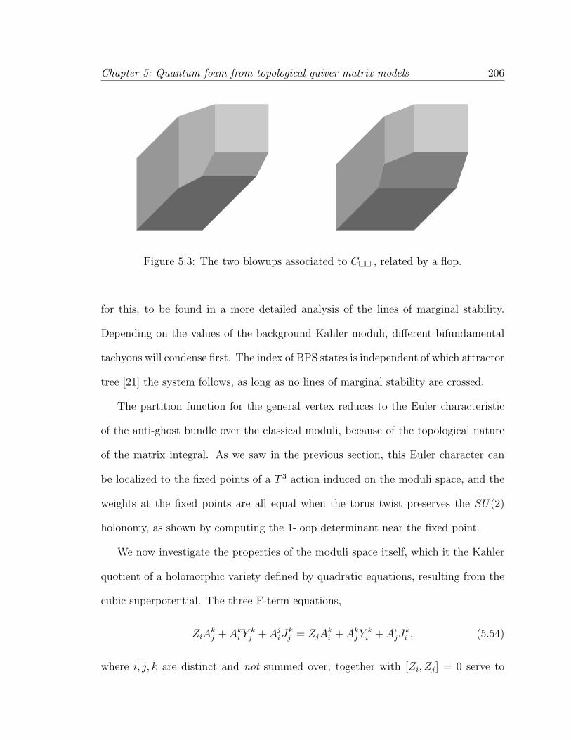
Chapter 5: Quantum foam from topological quiver matrix models 206
Figure 5.3: The two blowups associated to C¤¤·, related by a flop.
for this, to be found in a more detailed analysis of the lines of marginal stability.
Depending on the values of the background Kahler moduli, different bifundamental
tachyons will condense first. The index of BPS states is independent of which attractor
tree [21] the system follows, as long as no lines of marginal stability are crossed.
The partition function for the general vertex reduces to the Euler characteristic
of the anti-ghost bundle over the classical moduli, because of the topological nature
of the matrix integral. As we saw in the previous section, this Euler character can
be localized to the fixed points of a T 3 action induced on the moduli space, and the
weights at the fixed points are all equal when the torus twist preserves the SU(2)
holonomy, as shown by computing the 1-loop determinant near the fixed point.
We now investigate the properties of the moduli space itself, which it the Kahler
quotient of a holomorphic variety defined by quadratic equations, resulting from the
cubic superpotential. The three F-term equations,
ZiAkj + Ak
i Ykj + Aj
iJkj = ZjA
ki + Ak
j Yki + Ai
jJki , (5.54)
where i, j, k are distinct and not summed over, together with [Zi, Zj] = 0 serve to

Chapter 5: Quantum foam from topological quiver matrix models 207
define the holomorphic moduli space of the dynamical low energy degrees of freedom.
In our noncompact setup, we have not specified the boundary conditions for the 2-
branes, which are frozen in the local analysis. If they are free to move in the transverse
directions, generically they will not intersect, and the effective geometry probed by a
BPS 0-brane will be the blowup along the wrapped 2-cycles, as can be seen by going
to a complex basis in which Zi and Aij are all diagonal. The 2-2’ strings will become
massive, and exit the low energy spectrum, when the branes are separated, and (5.54)
becomes k1 + k2 + k3 equations describing the local geometry C×O(−1) → P1 near
each of the blown up 2-cycles.
It is also very interesting to consider compactifications in which the D2 branes
wrap rigid or obstructed 2-cycles. In that case, they will have a nontrivial intersec-
tion, and a more sophisticated analysis is needed. As we will show in the following
examples, the effective geometry is again the blow up along the wrapped subschemes.
It is here that multiple smooth resolutions of the geometry may exist, corresponding
to different attractor trees in which the order in which the tachyonic fields condense
changes. No walls of marginal stability are crossed, hence the index of BPS remains
constant.
The supersymmetric bound states we are discussing only exist when the asymp-
totic B-field is sufficiently large. From the perspective of Minkowski space, as the
B-field flow down to the attractor value, various walls of marginal stability will be
crossed. Thus the full geometry is multi-centered. Certain features of the attrac-
tor flow tree are visible in the quiver matrix model, so we first examine them from
supergravity.

Chapter 5: Quantum foam from topological quiver matrix models 208
The central charge of a D6/D4/D2/D0 bound state described by a complex of
sheaves E∗ over the Calabi-Yau is, at large radius,
Z(E∗) =
∫e−ωch(E∗)
√Td(X), (5.55)
where ω = B + iJ is the Kahler (1, 1)-form on X [9]. At small volumes, this would
receive worldsheet instanton corrections, hence the following analysis should only be
expected to indicate the qualitative behavior of the attractor flow. This is sufficient
for our purposes, since the local limit automatically assumes large volume.
In our case of ki 2-branes and N 0-branes bound to a D6 brane in the equivariant
vertex, the central charge (5.55) is computed as
∫e
∑tiωi (1 + k1ω2 ∧ ω3 + k2ω1 ∧ ω3 + k3ω1 ∧ ω2 + Nω1 ∧ ω2 ∧ ω3) = t1t2t3+
∑tiki+N,
(5.56)
where the ti are Kahler parameters associated to toric legs. They may be independent
or obey some relations, depending on the embedding of the vertex into a compact
3-fold.
From this one can check the well known fact that the 6-0 BPS bound state only
exists when arg(t3) > 0, that is |Bzz| >(1/√
3) |gzz|. Similar calculations have
been done in [21] when there are also D2 branes. We are most interested in the
behavior of the 2-branes as the moduli approach the attractor values. Note that in
a local analysis, the attractor flow itself cannot be determined without knowing the
compactification; this is obvious because when the ti become small, the vertex is no
longer a good approximation.
All of these details of the global geometry are hidden in the FI parameters and
the VEVs of the frozen fields appearing in the effective action for the 0-brane degrees

Chapter 5: Quantum foam from topological quiver matrix models 209
of freedom. This is consistent with the expectation that the theory is defined at
the asymptotic values of the moduli, where the 2-brane fields are heavy and their
fluctuations about the frozen values can be integrated out. The topological nature of
the matrix models guarantees that the only effect will be a ratio 1-loop determinants,
which in fact cancel up to a sign.
As the moduli flow according to the attractor equations from the large B-field
asymptotic limit needed to support the 6-brane BPS states, there are various possible
decays. To find the walls along which they occur, one finds the condition for the
central charges of the potential fragments to align. We find that in our examples, the
0-branes first split off.
The remaining D6/D2 bound state will itself decay at another wall of marginal
stability. Depending on the asymptotic value of the moduli, the 2-branes wrapped
one of the three toric legs will fragment off. Because the relevant Kahler moduli space
is six real dimensional even in the local context, the full stability diagram is difficult
to depict on paper, so we will content ourselves with the representative cross-section
shown in Figure 5.4. The charges in this example are denoted by
Γ = ω1 ∧ ω2 ∧ ω3 + ω1 + ω2 + 1
Γ6/2 = ω1 ∧ ω2 ∧ ω3 + ω1 + ω2
Γ1 = ω1
Γ2 = ω2.
We choose the background Kahler moduli to be
t1 = 16i + x, t2 = 14i + y, t3 = 4i + 4,

Chapter 5: Quantum foam from topological quiver matrix models 210
20 40 60 80
20
40
60
80
Figure 5.4: Walls of marginal stability for the decays Γ → Γ0 + Γ6/2 (dashed line),Γ6/2 → Γ1 + Γ′ (dotted), and Γ6/2 → Γ2 + Γ′′ (solid).
and plot the x, y plane which parameterizes the asymptotic value of the B-field along
the curves wrapped by the D2 branes.
It is immediately apparent that as the B-field in the z1 and z2 planes decrease
along the attractor flow, the 0-branes separate along the first curve shown, and then
the D6/D2 fragment intersects one of the two 2-brane curves. We shall see below how
this phenomenon is imprinted on the matrix model. Therefore, in our local analysis,
the 2-brane degrees of freedom are frozen in a pattern which depends on the attractor
flow tree. It is natural that the indices calculated for the different effective 0-brane
geometries are equal, since we see that they arise from the same theory in the global
Calabi-Yau geometry.
5.5.1 Probing the effective geometry of a single 2-brane with
N 0-branes
Let us first understand a very simple example from this point of view, namely the
effective geometry induced by a single D2 brane, corresponding to the vertex C¤··.

Chapter 5: Quantum foam from topological quiver matrix models 211
Consider probing the induced geometry wrapped by the D6 brane using N 0-branes.
The F-term equation (5.44) tells us that Z1A2 = Z2A1, where we set the D2 position
to 0 without loss of generality. Ignoring the z3 direction for now, as it simply goes
along for the ride, we see that this can be related to the quiver for a D4/D2/D0
bound state in O(−1) → P1, which lifts to D6/D4/D0 in the three dimensional blow
up. The D4 brane is equivalent to the line bundle mentioned before, since it can be
dissolved into smooth flux on the 6-brane worldvolume.
To see this, consider the two node quiver for O(−1) → P1 obtained by dropping
one dimension from the quiver of resolved conifold. Setting the field D = (I0) for
quiver charges N and N +1 splits U(N +1) → U(N)×U(1), and allows one to define
Za = CaD, (5.57)
and Aa to the be the U(1) piece of Ca. Then the relation C1BC2 = C2BC1 implies
that Z1A2 = Z2A1 and [Z1, Z2] = 0, as desired.
The two moduli spaces are not quite identical, however, because it is not always
possible to choose a gauge such that D = (I 0), and conversely, given such a form
for D, it is impossible to satisfy the D-term condition when Za = 0. Therefore the
structure of the moduli spaces near the zero section of O(−1) differ. In particular, it
is easy to see that if Z1 = Z2 = 0 in some M dimensional subspace of CN then there
is a P1 of A1, A2 if M = 1, a single point if M = 2, and a violation of the D-term if
M > 2. This is the sense in which the resolution is small - only a single 0-brane can
fit conformably.
Lifting to the full C3 adds one complex dimension to the 2-brane, hence the even
far from the exceptional divisor the 0-branes will see a U(1) flux turned on in the D6

Chapter 5: Quantum foam from topological quiver matrix models 212
gauge theory. This has no effect on the moduli space of a single BPS D0, but will
twist the global structure of the N D0 moduli space as follows.
Ordinarily, the Hilbert scheme of points is a kind of non-smooth “resolution”
of the classical space of N points in a 3-fold, SymN(X). For simplicity, consider
the case of Sym2(X), which looks like the bundle T /Z2 → ∆ near the diagonal
embedding, ∆ : X → Sym2 X, where T is the tangent bundle, with the natural Z2
action zi → −zi in local coordinates on the fiber. The zi should be thought of as the
small relative separation of the two points. In this special case, the Hilbert scheme
Hilb2(X), is locally the smooth resolution of the Z2 orbifold, which replaces the fiber
by O(−2) → P2.
Therefore near the diagonal, the Hilbert scheme of two points on X is given by
O(−2)⊗K −→ PT
↓
X,
where the O(−2) bundle is fibered trivially over the base, and K is the canonical
bundle over X. When a U(1) flux on the D6 worldvolume is turned on, carrying D4
charge, the O(−2) of the Hilbert scheme becomes fibered over the diagonal in the
sense of L, the U(1) bundle over X. That is, we should write LX ⊗ KX ⊗ O(−2)P2
in the above diagram of the geometry where the points are close together. This
is compactified in a natural way to the full Hilbert scheme with a background line
bundle, and a similar situation holds for N > 2 D0 branes.
Intriguingly, the effective canonical class of X, in the sense of the what line bundle
appears in the above description of the Hilbert scheme, turns out to be the trivial

Chapter 5: Quantum foam from topological quiver matrix models 213
bundle in our case, since L exactly cancels the fibration of K by the nature of the blow
up construction. It would be interesting to understand if there is any more robust
way in which the blow ups are effectively Calabi-Yau.
5.5.2 Example 2: the geometry of C¤¤·
Let us work out the example of C¤¤· in detail, as it already possesses most of the
new features. The classical moduli of the D2 branes are the coordinates y12, y
13 and
y21, y
23 respectively. Depending on the details of the compactification, which determine
the superpotential for these fields, it may be possible to separate the branes in the
z3 direction. In that case, the 2-2’ strings develop a mass and exit the low energy
spectrum. Hence N probe D0 branes will have a BPS moduli space given by the
U(1)2 × SU(N) Kahler quotient of
(Z2 − y1
2
)A1
3 =(Z3 − y1
3
)A1
2
(Z1 − y2
1
)A2
3 =(Z3 − y2
3
)A2
1
[Zi, Zj] = 0.
(5.58)
For y13 6= y2
3, this looks locally, near each of the D2 branes, like the geometry of N D0
branes in the “small” blowup discussed before. In particular, a single D0 probe sees
exactly the blow up geometry along the two disjoint curves.
More interesting behavior occurs when the 2-branes cannot be separated in this
way, for example in the closed vertex geometry in which the wrapped P1’s are rigid.
This is more closely connected with the equivariant result, which requires the wrapped
2-cycles to have such a non-generic intersection by torus invariance. Here we must

Chapter 5: Quantum foam from topological quiver matrix models 214
use the fact that
J ij
(Ai
j
)†= 0, (5.59)
which results from the term (5.50) in the effective action.
The effective geometry of the C¤¤· vertex, as probed by an individual BPS D0
brane is therefore determined by the Kahler quotient of the variety ,
z2a13 = a2
3j12
z1a23 = z3a
21,
(5.60)
by U(1)× U(1) under which the fields have charges
zi a13 j1
2 a21 a2
3
0 1 1 0 0
0 1 −1 1 1
The first equation implies that (z2, a23) lives in the O(−1) bundle over the P1 with
homogeneous coordinates (a13 : j1
2). Moreover the second equation fixes (z1, z3) to be
fibered in O(−1) on the compactification of the a23 direction. This is shown in the
toric diagram (see Figure 5.3), which is exactly the resolution of the blow up of C3
along the non-generically intersecting z1 and z2 lines!
Reversing the roles of the two D2 branes will result in a flopped geometry (which in
this case is coincidentally geometrically equivalent to the first). It seems reasonable
to conjecture that as one dials the background moduli, and thus implicitly the FI
parameters, such that the roles of the two branes are exchanged, the attractor tree
pattern changes without crossing a wall of marginal stability. This behavior was
observed in a related system in [21]. We are using the intuitive identification between
the attractor flow and the line of quickest descent in the potential of the matrix model.

Chapter 5: Quantum foam from topological quiver matrix models 215
5.5.3 An example with three 2-branes
The blowup of the vertex geometry along all three torus invariant legs has a total
of four smooth resolutions, related by conifold flops. This is the right description
when the legs are expected to become rigid spheres in the global geometry, so they
cannot be holomorphically deformed away from the triple intersection. Let us see
explicitly how one of these blowups arises from the quiver description of C¤¤¤.
Suppose that the 2-brane wrapping the z1 plane has melted first into the back-
ground D6, that is, I1 6= 0. Without any 0-brane probes, the dynamical fields are the
J ij , which satisfy F-term conditions derived before requiring that J i
jJji = 0, J i
jJki = 0,
and J ijI
i = 0 for all distinct i, j, k. It is easy to satisfy the D-term constrain, for
appropriate values of the FI parameters, by taking J21 , J3
1 6= 0 and all others vanish-
ing. These can be gauged away using the U(1)’s associated to the D2 worldvolumes,
as expected, therefore the BPS configuration is completely determined by the frozen
fields, and the moduli space is a point.
Probing this system with a D0 brane, we find that ∂W = 0 implies
z1a23 = a1
3j21
z2a13 = z3a
12
z1a32 = a1
2j31 .
The Kahler structure is determined by the D-terms,
|J21 |2 + |J3
1 |2 − |a13|2 − |a1
2|2 = r1
|J21 |2 + |a2
3|2 = r2
|J31 |2 + |a3
2|2 = r3,

Chapter 5: Quantum foam from topological quiver matrix models 216
Figure 5.5: Toric diagrams of some blowups associated to C¤¤¤, related by flops.
where we have absorbed the contributions of the frozen degrees of freedom associated
to noncompactness into the FI parameters. Completing the Kahler quotient by U(1)3,
one obtains the toric web diagram shown in Figure 5.5.
As we have seen before, the fact that the Euler character is 4 instead of the
expected 3 is not a contradiction, since if r1 > 0, than one of the Ja1 6= 0, and the
central P1 gets shrunken to a point. It is reasonable to expect that this is not a wall of
marginal stability, but rather a change in the attractor tree pattern, since the Ja1 = 0
branch of the moduli space for r1 < 0 is connected to the configurations in which
the 2-branes are separated. If that was the case, then a full analysis of the fermionic
terms in the matrix model would show that the anti-ghost bundle is not the tangent
bundle in this case, and only contributes 1 from the resolved P1. This seems more
natural than a true jump in the index, because the r1 > 0 classical moduli space is
singular, and one would expect an Euler character of 2 from the conifold singularity
if we were using the tangent bundle.
The other resolutions of the blow up are also related by changing the pattern of

Chapter 5: Quantum foam from topological quiver matrix models 217
the attractor flow, condensing first one of the other 2-6 tachyons. These are related
geometrically via flops through the symmetric resolution shown in Figure 5.5.
5.6 Conclusions and further directions
We constructed matrix models possessing a topological supersymmetry from the
quiver descriptions of holomorphic branes in a Calabi-Yau by adding the associated
fermions, introducing the multiplets resulting from motion in the Minkowski direc-
tions, and imposing the constraints using the anti-ghost field method of [70]. These
matrix models are the topologically twisted version of the D-brane theory in the ex-
treme IR limit; that is, they are theories of the BPS sector of the (unknown) dual
superconformal quantum mechanics.
The partition function was shown to localize to the Euler character of an obstruc-
tion bundle over the classical moduli, by proving the appropriate vanishing theorems.
We evaluated the partition function by regularizing the path integral by gauging part
of the U(1)3 torus symmetry, and using the localization of this equivariant version to
the fixed points of the torus action, giving exact agreement with known results.
The toric vertex geometry we studied can be obtained as the local limit of various
compact Calabi-Yau manifolds. The T 3 symmetry guarantees that the information of
the global geometry only affects the local degrees of freedom that remain dynamical
in the limit through the values of the FI parameters and the background VEVs of
certain frozen fields. Quite generally, some gauge groups of global quiver will be
broken by the frozen VEVs, and the associated residual off-diagonal components of
the D-term can appear in the effective matrix model.

Chapter 5: Quantum foam from topological quiver matrix models 218
We saw that the geometry of the BPS moduli space of a single 0-brane in a D6/D2
background in the vertex is exactly the blowup along the curves wrapped by the 2-
branes. The structure of the moduli space of N probe 0-branes was also investigated,
revealing interesting behavior. This can be viewed as a first step in embedding the
quantum foam picture of the A-model into the full IIA theory. In particular we found
that effective internal geometry seen by 0-brane probes is indeed the blow ups of the
Calabi-Yau predicted in [37].
It might be interesting to relate these ideas to the open/closed duality discussed in
[29]. Although the discussion there is in the context of finding the closed string dual
of Lagrangian branes in the A-model, they find a sum over Calabi-Yau geometries
that depend on which term one one looks at in the Young diagram expansion of the
open string holonomy. From the quantum foam point of view, these are related to the
2-brane bound states, so there could be some connection to the effective geometries
we have investigated.
In this paper we have focused on the quiver for Donaldson-Thomas theory in the
vertex geometry, but the extension of these ideas to many toric geometries should
be straightforward. Likewise, even the bound states of branes on a compact Calabi-
Yau such as the quintic, which have a quiver description, may be computed using
similar topological matrix models. In those cases, the technical difficulty of finding
all of the fixed points of a toric action on the classical BPS moduli space increases
proportionally. Therefore the hope would be to find a way around performing the
direct evaluation used here.
It would be very interesting to try to apply the techniques of matrix models at

Chapter 5: Quantum foam from topological quiver matrix models 219
large N to the quiver theories constructed here. It is natural to expect that an
intriguing structure should emerge in the expansion about that large charge limit.
This would make sharp the idea that these matrix models give the “CFT” dual of the
square of the topological string, at least in the OSV regime, since one would identify
the perturbative topological string expansion with the 1/N corrections in the quiver
matrix model.
Closer to the topic of the 6-brane theories studied in this paper, one would also
hope to find a large charge expansion describing the analog of the limit shapes in [60].
The quiver theories would contain further information about the large charge moduli
space away from the torus fixed points. Such a method of finding the asymptotic
expansion of the partition function could have implications for the entropy enigma
found in [21]. On the other hand, because our matrix models are topological, the
naive perturbative expansion is trivial, cancelling between bosons and fermions, so
novel techniques would be required to obtain the large N limit.

Bibliography
[1] Mina Aganagic, Robbert Dijkgraaf, Albrecht Klemm, Marcos Marino, and Cum-run Vafa. Topological strings and integrable hierarchies. Commun. Math. Phys.,261:451–516, 2006.
[2] Mina Aganagic, Daniel Jafferis, and Natalia Saulina. Branes, black holes andtopological strings on toric calabi-yau manifolds. JHEP, 12:018, 2006.
[3] Mina Aganagic, Albrecht Klemm, Marcos Marino, and Cumrun Vafa. Matrixmodel as a mirror of chern-simons theory. JHEP, 02:010, 2004.
[4] Mina Aganagic, Albrecht Klemm, Marcos Marino, and Cumrun Vafa. The topo-logical vertex. Commun. Math. Phys., 254:425–478, 2005.
[5] Mina Aganagic, Marcos Marino, and Cumrun Vafa. All loop topological stringamplitudes from chern-simons theory. Commun. Math. Phys., 247:467–512, 2004.
[6] Mina Aganagic, Andrew Neitzke, and Cumrun Vafa. Bps microstates and theopen topological string wave function. 2005.
[7] Mina Aganagic, Hirosi Ooguri, Natalia Saulina, and Cumrun Vafa. Black holes,q-deformed 2d yang-mills, and non-perturbative topological strings. Nucl. Phys.,B715:304–348, 2005.
[8] Xerxes Arsiwalla, Rutger Boels, Marcos Marino, and Annamaria Sinkovics.Phase transitions in q-deformed 2d yang-mills theory and topological strings.Phys. Rev., D73:026005, 2006.
[9] Paul S. Aspinwall. D-branes on calabi-yau manifolds. 2004.
[10] Paul S. Aspinwall and Lukasz M. Fidkowski. Superpotentials for quiver gaugetheories. JHEP, 10:047, 2006.
[11] M. F. Atiyah, Nigel J. Hitchin, V. G. Drinfeld, and Yu. I. Manin. Constructionof instantons. Phys. Lett., A65:185–187, 1978.
[12] Tom Banks, W. Fischler, S. H. Shenker, and Leonard Susskind. M theory as amatrix model: A conjecture. Phys. Rev., D55:5112–5128, 1997.
220

Bibliography 221
[13] M. Bershadsky, S. Cecotti, H. Ooguri, and C. Vafa. Kodaira-spencer theory ofgravity and exact results for quantum string amplitudes. Commun. Math. Phys.,165:311–428, 1994.
[14] M. Bershadsky, C. Vafa, and V. Sadov. D-branes and topological field theories.Nucl. Phys., B463:420–434, 1996.
[15] Nicola Caporaso et al. Topological strings and large n phase transitions. ii: Chiralexpansion of q-deformed yang-mills theory. JHEP, 01:036, 2006.
[16] Stefan Cordes, Gregory W. Moore, and Sanjaye Ramgoolam. Lectures on 2-dyang-mills theory, equivariant cohomology and topological field theories. Nucl.Phys. Proc. Suppl., 41:184–244, 1995.
[17] Atish Dabholkar. Exact counting of black hole microstates. Phys. Rev. Lett.,94:241301, 2005.
[18] Atish Dabholkar, Frederik Denef, Gregory W. Moore, and Boris Pioline. Exactand asymptotic degeneracies of small black holes. JHEP, 08:021, 2005.
[19] Atish Dabholkar, Frederik Denef, Gregory W. Moore, and Boris Pioline. Preci-sion counting of small black holes. JHEP, 10:096, 2005.
[20] Sebastian de Haro and Miguel Tierz. Discrete and oscillatory matrix models inchern-simons theory. Nucl. Phys., B731:225–241, 2005.
[21] Frederik Denef and Gregory W. Moore. Split states, entropy enigmas, holes andhalos. 2007.
[22] Robbert Dijkgraaf, Rajesh Gopakumar, Hirosi Ooguri, and Cumrun Vafa. Babyuniverses in string theory. Phys. Rev., D73:066002, 2006.
[23] Robbert Dijkgraaf and Cumrun Vafa. Matrix models, topological strings, andsupersymmetric gauge theories. Nucl. Phys., B644:3–20, 2002.
[24] Robbert Dijkgraaf, Cumrun Vafa, and Erik Verlinde. M-theory and a topologicalstring duality. 2006.
[25] Michael R. Douglas. D-branes, categories and n = 1 supersymmetry. J. Math.Phys., 42:2818–2843, 2001.
[26] Michael R. Douglas, Brian R. Greene, and David R. Morrison. Orbifold resolutionby d-branes. Nucl. Phys., B506:84–106, 1997.
[27] Michael R. Douglas and Vladimir A. Kazakov. Large n phase transition incontinuum qcd in two- dimensions. Phys. Lett., B319:219–230, 1993.

Bibliography 222
[28] Davide Gaiotto, Andrew Strominger, and Xi Yin. Superconformal black holequantum mechanics. JHEP, 11:017, 2005.
[29] Jaume Gomis and Takuya Okuda. D-branes as a bubbling calabi-yau. 2007.
[30] David J. Gross. Two-dimensional qcd as a string theory. Nucl. Phys., B400:161–180, 1993.
[31] David J. Gross and Andrei Matytsin. Instanton induced large n phase transitionsin two- dimensional and four-dimensional qcd. Nucl. Phys., B429:50–74, 1994.
[32] David J. Gross and IV Taylor, Washington. Twists and wilson loops in the stringtheory of two- dimensional qcd. Nucl. Phys., B403:395–452, 1993.
[33] David J. Gross and IV Taylor, Washington. Two-dimensional qcd is a stringtheory. Nucl. Phys., B400:181–210, 1993.
[34] Grothendieck. Theorie des intersections et theoreme de Riemann-Roch.Springer-Verlag, Berlin, 1971. Seminaire de Geometrie Algebrique du Bois-Marie1966–1967 (SGA 6), Dirige par P. Berthelot, A. Grothendieck et L. Illusie. Avecla collaboration de D. Ferrand, J. P. Jouanolou, O. Jussila, S. Kleiman, M. Ray-naud et J. P. Serre, Lecture Notes in Mathematics, Vol. 225.
[35] Monica Guica and Andrew Strominger. Cargese lectures on string theory witheight supercharges. 2007.
[36] Nick Halmagyi, Annamaria Sinkovics, and Piotr Sulkowski. Knot invariants andcalabi-yau crystals. JHEP, 01:040, 2006.
[37] Amer Iqbal, Nikita Nekrasov, Andrei Okounkov, and Cumrun Vafa. Quantumfoam and topological strings. 2003.
[38] Daniel Jafferis. Crystals and intersecting branes. 2006.
[39] J. P. Jouanolou. Riemann-Roch sans denominateurs. Invent. Math., 11:15–26,1970.
[40] Igor R. Klebanov and Edward Witten. Superconformal field theory on three-branes at a calabi-yau singularity. Nucl. Phys., B536:199–218, 1998.
[41] C. Klimcik. The formulae of kontsevich and verlinde from the perspective of thedrinfeld double. Commun. Math. Phys., 217:203–228, 2001.
[42] Alexander A. Klyachko. Vector bundles and torsion free sheaves on the projectiveplane. Preprint Max Planck Institut fur Mathematik, 1991.

Bibliography 223
[43] Alexander A. Klyachko. Stable bundles, representation theory and hermitianoperators. Selecta Mathematica, New Series, 4:419 – 445, 1998.
[44] J. M. F. Labastida and Carlos Lozano. The vafa-witten theory for gauge groupsu(n). Adv. Theor. Math. Phys., 3:1201–1225, 1999.
[45] Gabriel Lopes Cardoso, Bernard de Wit, and Thomas Mohaupt. Correctionsto macroscopic supersymmetric black-hole entropy. Phys. Lett., B451:309–316,1999.
[46] Gabriel Lopes Cardoso, Bernard de Wit, and Thomas Mohaupt. Deviations fromthe area law for supersymmetric black holes. Fortsch. Phys., 48:49–64, 2000.
[47] Gabriel Lopes Cardoso, Bernard de Wit, and Thomas Mohaupt. Macroscopic en-tropy formulae and non-holomorphic corrections for supersymmetric black holes.Nucl. Phys., B567:87–110, 2000.
[48] T. Okuda M. Aganagic, H. Ooguri. to appear.
[49] Juan M. Maldacena, Andrew Strominger, and Edward Witten. Black hole en-tropy in m-theory. JHEP, 12:002, 1997.
[50] Marcos Marino. Chern-simons theory, matrix integrals, and perturbative three-manifold invariants. Commun. Math. Phys., 253:25–49, 2004.
[51] Marcos Marino. Les houches lectures on matrix models and topological strings.2004.
[52] D. Maulik, N. Nekrasov, A. Okounkov, and R. Pandharipande. Gromov-wittentheory and donaldson-thomas theory, ii, 2004.
[53] J. A. Minahan, D. Nemeschansky, C. Vafa, and N. P. Warner. E-strings and n= 4 topological yang-mills theories. Nucl. Phys., B527:581–623, 1998.
[54] Joseph A. Minahan and Alexios P. Polychronakos. Classical solutions for two-dimensional qcd on the sphere. Nucl. Phys., B422:172–194, 1994.
[55] Gregory W. Moore, Nikita Nekrasov, and Samson Shatashvili. D-particle boundstates and generalized instantons. Commun. Math. Phys., 209:77–95, 2000.
[56] Gregory W. Moore, Nikita Nekrasov, and Samson Shatashvili. Integrating overhiggs branches. Commun. Math. Phys., 209:97–121, 2000.
[57] H. Nakajima. Lectures on Hilbert Schemes of Points on Surfaces. AmericanMathematical Society, 1999.

Bibliography 224
[58] Hiraku Nakajima. Instantons on ALE spaces, quiver varieties, and Kac-Moodyalgebras. Duke Math. J., 76(2):365–416, 1994.
[59] A. Okounkov and N. Rechetikhin. Correlation function of schur process withapplication to local geometry of a random 3-dimensional young diagram. J.Amer. Math. Soc., 16:581–603, 2003.
[60] Andrei Okounkov, Nikolai Reshetikhin, and Cumrun Vafa. Quantum calabi-yauand classical crystals. 2003.
[61] Takuya Okuda. Derivation of calabi-yau crystals from chern-simons gauge theory.JHEP, 03:047, 2005.
[62] Hirosi Ooguri, Andrew Strominger, and Cumrun Vafa. Black hole attractors andthe topological string. Phys. Rev., D70:106007, 2004.
[63] Kirill Saraikin and Cumrun Vafa. Non-supersymmetric black holes and topolog-ical strings. 2007.
[64] Ashoke Sen. Black holes and the spectrum of half-bps states in n = 4 supersym-metric string theory. Adv. Theor. Math. Phys., 9:527–558, 2005.
[65] Ashoke Sen. Black holes, elementary strings and holomorphic anomaly. JHEP,07:063, 2005.
[66] David Shih and Xi Yin. Exact black hole degeneracies and the topological string.JHEP, 04:034, 2006.
[67] Washington Taylor. Counting strings and phase transitions in 2-d qcd. 1994.
[68] Cumrun Vafa. Instantons on d-branes. Nucl. Phys., B463:435–442, 1996.
[69] Cumrun Vafa. Two dimensional yang-mills, black holes and topological strings.2004.
[70] Cumrun Vafa and Edward Witten. A strong coupling test of s duality. Nucl.Phys., B431:3–77, 1994.
[71] Edward Witten. Quantum background independence in string theory. 1993.
[72] Edward Witten. Bps bound states of d0-d6 and d0-d8 systems in a b-field. JHEP,04:012, 2002.


![Topological Effects of D-brane Charges in String Theory · I K-theory enters in defining the RR-charges in Type I and II superstring theories [Minasian and Moore 1997]. I Constructed](https://static.fdocuments.in/doc/165x107/5f34c372cc92bb138b27217d/topological-eiects-of-d-brane-charges-in-string-theory-i-k-theory-enters-in-deining.jpg)

