Topological Ramsey numbers and countable ordinals Ramsey numbers and countable ordinals Andr es...
32
Contemporary Mathematics Topological Ramsey numbers and countable ordinals Andr´ es Eduardo Caicedo and Jacob Hilton To W. Hugh Woodin, on the occasion of his birthday. Abstract. We study the topological version of the partition calculus in the setting of countable ordinals. Let α and β be ordinals and let k be a positive integer. We write β →top (α, k) 2 to mean that, for every red-blue coloring of the collection of 2-sized subsets of β, there is either a red-homogeneous set homeomorphic to α or a blue-homogeneous set of size k. The least such β is the topological Ramsey number R top (α, k). We prove a topological version of the Erd˝os-Milner theorem, namely that R top (α, k) is count- able whenever α is countable. More precisely, we prove that R top (ω ω β ,k + 1) ≤ ω ω β·k for all countable ordinals β and finite k. Our proof is modeled on a new easy proof of a weak version of the Erd˝os-Milner theorem that may be of independent interest. We also provide more careful upper bounds for certain small values of α, proving among other results that R top (ω +1,k + 1) = ω k + 1, R top (α, k) <ω ω whenever α<ω 2 , R top (ω 2 ,k) ≤ ω ω and R top (ω 2 +1,k + 2) ≤ ω ω·k + 1 for all finite k. Our computations use a variety of techniques, including a topological pigeonhole principle for ordinals, considerations of a tree ordering based on the Cantor normal form of ordinals, and some ultrafilter arguments. Contents 1. Introduction 2 2. Preliminaries 6 3. The closed pigeonhole principle for ordinals 7 4. The ordinal ω +1 10 5. Stepping up by one 11 6. Ordinals less than ω 2 15 7. The ordinal ω 2 18 8. The anti-tree partial ordering on ordinals 19 9. The ordinal ω 2 +1 24 2010 Mathematics Subject Classification. Primary 03E02. Secondary 03E10, 54A25. Key words and phrases. Partition calculus, countable ordinals. The second author’s research was conducted under the supervision of John K. Truss with the support of an EPSRC Doctoral Training Grant Studentship. c 0000 (copyright holder) 1 arXiv:1510.00078v3 [math.LO] 9 Apr 2017
Transcript of Topological Ramsey numbers and countable ordinals Ramsey numbers and countable ordinals Andr es...

Contemporary Mathematics
Topological Ramsey numbers and countable ordinals
Andres Eduardo Caicedo and Jacob Hilton
To W. Hugh Woodin, on the occasion of his birthday.
Abstract. We study the topological version of the partition calculus in the setting of countable
ordinals. Let α and β be ordinals and let k be a positive integer. We write β →top (α, k)2 tomean that, for every red-blue coloring of the collection of 2-sized subsets of β, there is either a
red-homogeneous set homeomorphic to α or a blue-homogeneous set of size k. The least such βis the topological Ramsey number Rtop(α, k).
We prove a topological version of the Erdos-Milner theorem, namely that Rtop(α, k) is count-
able whenever α is countable. More precisely, we prove that Rtop(ωωβ , k + 1) ≤ ωωβ·k for all
countable ordinals β and finite k. Our proof is modeled on a new easy proof of a weak version of
the Erdos-Milner theorem that may be of independent interest.We also provide more careful upper bounds for certain small values of α, proving among other
results that Rtop(ω + 1, k + 1) = ωk + 1, Rtop(α, k) < ωω whenever α < ω2, Rtop(ω2, k) ≤ ωω
and Rtop(ω2 + 1, k + 2) ≤ ωω·k + 1 for all finite k.Our computations use a variety of techniques, including a topological pigeonhole principle
for ordinals, considerations of a tree ordering based on the Cantor normal form of ordinals, and
some ultrafilter arguments.
Contents
1. Introduction 22. Preliminaries 63. The closed pigeonhole principle for ordinals 74. The ordinal ω + 1 105. Stepping up by one 116. Ordinals less than ω2 157. The ordinal ω2 188. The anti-tree partial ordering on ordinals 199. The ordinal ω2 + 1 24
2010 Mathematics Subject Classification. Primary 03E02. Secondary 03E10, 54A25.Key words and phrases. Partition calculus, countable ordinals.The second author’s research was conducted under the supervision of John K. Truss with the support of an
EPSRC Doctoral Training Grant Studentship.
c©0000 (copyright holder)
1
arX
iv:1
510.
0007
8v3
[m
ath.
LO
] 9
Apr
201
7
2 ANDRES EDUARDO CAICEDO AND JACOB HILTON
10. The weak topological Erdos-Milner theorem 2611. Questions 29References 30
1. Introduction
Motivated by Ramsey’s theorem, the partition calculus for cardinals and Rado’s arrow notationwere introduced by Erdos and Rado in [ER53]. The version for ordinals, where the homogeneousset must have the correct order type, first appears in their seminal paper [ER56]. In the followingdefinition, [X]n denotes the set of subsets of X of size n.
Definition 1.1. Let κ be a cardinal, let n be a positive integer, and let β and all αi be ordinalsfor i ∈ κ. We write
β → (αi)ni∈κ
to mean that for every function c : [β]n → κ (a coloring) there exists some subset X ⊆ β and somei ∈ κ such that X is an i-homogeneous copy of αi, i.e., [X]n ⊆ c−1({i}) and X is order-isomorphicto αi.
This relation has been extensively studied, particularly the case n = 2, where we define the(classical) ordinal Ramsey number R(αi)i∈κ to be the least ordinal β such that β → (αi)
2i∈κ.
Ramsey’s theorem can be stated using this notation as R(ω, ω) = ω.A simple argument that goes back to Sierpinski shows that β 6→ (ω+ 1, ω)2 for every countable
ordinal β [Sie33], which means that if α > ω and R(α, γ) is countable, then γ must be finite (see also[ER56, Theorem 19] and [Spe57, Theorem 4]). On the other hand, Erdos and Milner showed thatindeed R(α, k) is countable whenever α is countable and k is finite [EM72]. Much work has beendone to compute these countable ordinal Ramsey numbers. In particular, as announced withoutproof by Haddad and Sabbagh [HS69c, HS69a, HS69b], there are algorithms for computingR(α, k) for several classes of ordinals α < ωω and all finite k; details are given in [Cai15] for thecase α < ω2 and in [Mil71] for the case α = ωm for finite m. See also [Wil77, Chapter 7], [HL10],[Sch10] and [Wei14].
With the development of structural Ramsey theory, many variants of the basic definition abovehave been introduced. In this article we are concerned with a “topological” version and a closely-related “closed” version. (Jean Larson suggested to call the second version “limit closed”.) Both ofthese make use of the topological structure of an ordinal, which we endow with the order topology.Although the second version may appear more natural, it is the first that has been consideredhistorically, since it can be defined for arbitrary topological spaces; the second version additionallyrequires an order structure.
In the following definition, ∼= denotes the homeomorphism relation. Following Baumgartner[Bau86], we also say that a subspace X of an ordinal is order-homeomorphic to an ordinal α tomean that there is a bijection X → α that is both an order-isomorphism and a homeomorphism,or equivalently, X is both order-isomorphic to α and closed in its supremum.
Definition 1.2. Let κ be a cardinal, let n be a positive integer, and let β and all αi be ordinalsfor i ∈ κ.
We write
β →top (αi)ni∈κ
TOPOLOGICAL RAMSEY NUMBERS 3
to mean that for every function c : [β]n → κ there exists some subspace X ⊆ β and some i ∈ κsuch that X is an i-homogeneous topological copy of αi, i.e., [X]n ⊆ c−1({i}) and X ∼= αi.
We write
β →cl (αi)ni∈κ
to mean that for every function c : [β]n → κ there exists some subset X ⊆ β and some i ∈ κ suchthat X is an i-homogeneous closed copy of αi, i.e., [X]n ⊆ c−1({i}) and X is order-homeomorphicto αi.
Note that in both cases, c is arbitrary (no continuity or definability is required).
The two versions coincide in many cases, in particular for ordinals of the form ωγ or ωγ ·m + 1 with m ∈ ω [Hil16, Theorem 2.16]. But in general they may differ; for example, ω + 2is homeomorphic but not order-homeomorphic to ω + 1, and thus ω + 1 →top (ω + 2)1
1 whileω + 1 6→cl (ω + 2)1
1.We focus primarily on the case n = 2, where we define the topological ordinal Ramsey number
Rtop(αi)i∈κ to be the least ordinal β (when one exists) such that β →top (αi)i∈κ, and the closedordinal Ramsey number Rcl(αi)i∈κ likewise. In particular, we study Rtop(α, k) and Rcl(α, k) whenα is a countable ordinal and k a positive integer, which have not previously been explored.
An important ingredient in our work is the case n = 1, which was first studied by Baumgartnerand Weiss [Bau86]. Analogously to Ramsey numbers, we define the pigeonhole number P (αi)i∈κto be the least ordinal β such that β → (αi)
1i∈κ, and we define the topological pigeonhole number
P top(αi)i∈κ and the closed pigeonhole number P cl(αi)i∈κ in a similar fashion. An algorithm forfinding the topological pigeonhole numbers is given in [Hil16], and we will describe the modificationsrequired to obtain the closed pigeonhole numbers (see Section 3). Repeatedly we make use of theclassical fact that the indecomposable ordinals, the powers of ω, satisfy P (ωα)k = ωα for all finitek.
Returning to the case n = 2, previous work has tackled uncountable Ramsey numbers. Erdosand Rado [ER56] showed that ω1 → (ω1, ω + 1)2. Laver noted in [Lav75] (and a proof, us-ing a pressing down argument, is described for example in [Sch12]) that one actually has ω1 →(Stationary, topω + 1)2, meaning that one can ensure either a 0-homogeneous stationary subset ora 1-homogeneous topological copy of ω+1. Since every stationary subset of ω1 contains topologicalcopies of every α ∈ ω1 [Fri74], this therefore shows that ω1 →top (α, ω+ 1)2 for all countable α. Inturn, this result was later extended by Schipperus using elementary submodel techniques to showthat ω1 →top (α)2
k for all α ∈ ω1 and all finite k [Sch12] (the topological Baumgartner-Hajnaltheorem). Meanwhile, both ω1 → (ω1, α)2 for all α ∈ ω1 [Tod83] and ω1 6→ (ω1, ω + 2)2 [Haj60]are consistent with ZFC, though the topological version of the former remains unchecked. Finally,it is also known that β 6→top (ω + 1)2
ℵ0 for all ordinals β [Wei90].When n > 2, not much more can be said in the setting of countable ordinals, since Kruse
showed that if n ≥ 3 and β is a countable ordinal, then β 6→ (ω + 1, n + 1)n [Kru65]. As forthe ordinal ω1, [ER56, Theorem 39 (ii)] shows that ω1 → (ω + 1)nk for all finite n, k and, in fact,it seems to be a folklore result that ω1 →top (ω + 1)nk for all finite n, k; a proof can be found in[HJW90]. On the other hand, we have the negative relations ω1 6→ (n + 1)nω for n ≥ 2 [ER56],ω1 6→ (ω+ 2, n+ 1)n for n ≥ 4 [Kru65], ω1 6→ (ω+ 2, ω)3 [Jon00] and ω1 6→ (ω1, 4)3 [Haj64]. Allthat remains to be settled is the conjecture that ω1 → (α, k)3 for all α ∈ ω1 and all finite k, withthe strongest result to date being that ω1 → (ω · 2 + 1, k)3 for all finite k [Jon17], building on thetechniques of [Tod83]. The topological version of this result remains unexplored. In a differentdirection, Rosenberg [Ros15] has recently verified that X →top (ω+ 1)nk for all finite n, k whenever

4 ANDRES EDUARDO CAICEDO AND JACOB HILTON
X is an uncountable separable metric space. Apparently, this last result has been discovered a fewtimes. In particular, Stevo Todorcevic has informed us that in unpublished work from around 1990,he and Weiss characterized those metric spaces X for which X →top (ω + 1)rk for all finite r, k. Healso provided us with a copy of his short unpublished note [Tod96] from 1996, where he shows thata regular space X with a point-countable basis is left-separated iff X 6→top (ω + 1)2
2 iff for someintegers r, k ≥ 2, X 6→top (ω + 1)rk.
For a general introduction to the partition calculus of countable ordinals, see [Cai14], whichalso provides some context for the work we present here. For a general introduction to topologicalRamsey theory, see [Wei90]. In a sense, [Bau86] is the direct precursor of this paper and [Hil16].Both authors were working independently on this topic when the talk on which [Cai14] is basedwas given. Upon learning of each other’s research, we decided to combine and extend our notes.Among other extensions, this resulted in the weak topological Erdos-Milner theorem.
1.1. Our results. Our main result is the weak topological Erdos-Milner theorem:
Theorem. Let α and β be countable nonzero ordinals, and let k > 1 be a positive integer. If
ωωα
→top (ωβ , k)2,
then
ωωα·β →top (ωβ , k + 1)2.
This is Theorem 10.2. Since trivially ωωα →top (ωω
α
, 2)2, it follows by induction on k that
Rtop(ωωα
, k + 1) ≤ ωωα·k
. Hence the ordinals Rtop(α, k) (and Rcl(α, k), since the two versionscoincide when α is a power of ω) are countable for all countable α and all finite k. (The reasonwhy we use here the adjective weak is discussed in Section 10.)
The paper is organized as follows.Section 2 completes the preliminaries, including further details of the relationship between the
topological and closed partition relations.In Section 3 we introduce the case n = 1 and solve the closed pigeonhole principle for ordinals:
given a cardinal κ and an ordinal αi ≥ 2 for each i ∈ κ, we provide an algorithm to computeP cl(αi)i∈κ. This is presented in Theorem 3.2. (The corresponding result for P top, building on[Bau86, Theorem 2.3], is the main theorem of [Hil16].) We also prove a simple lower bound forRamsey numbers in terms of pigeonhole numbers, which remains our best lower bound with theexception of a couple of special cases.
In Section 4 we look at ω + 1 and prove Theorem 4.1:
Theorem. If k is a positive integer, then Rtop(ω + 1, k + 1) = Rcl(ω + 1, k + 1) = ωk + 1.
In Section 5 we describe several “stepping up” techniques, resulting in Propositions 5.1 and 5.5:
Theorem. Let α be a successor ordinal, and let k, m and n be positive integers with k ≥ 2.
(1) Rcl(α+ 1, k + 1) ≤ P cl(Rcl(α, k + 1), Rcl(α+ 1, k)) + 1.(2) Rcl(α+ 1, k + 1) ≤ P cl(Rcl(α, k + 1))k +Rcl(α+ 1, k).(3) Rcl(ω ·m+n+1, k+1) ≤ Rcl(ω ·m+1, k+1)+P cl((Rcl(ω ·m+n+1, k))2m, R(n, k+1)).
From these one may deduce upper bounds for Rcl(ω + n, k) for all finite n, k. We also indicatea lower bound in Lemma 5.3, yielding Rcl(ω + 2, 3) = ω2 · 2 + ω + 2.
In Section 6 we use the last of these techniques, which in turn utilizes an ultrafilter argument,to prove Theorem 6.1:

TOPOLOGICAL RAMSEY NUMBERS 5
Theorem. If k and m are positive integers, then Rtop(ω·m+1, k+1) = Rcl(ω·m+1, k+1) < ωω.
In fact, in each case the proof gives an explicit upper bound below ωω.The ultrafilter approach is then further refined in Section 7 to prove Theorem 7.1:
Theorem. If k is a positive integer, then Rtop(ω2, k) = Rcl(ω2, k) ≤ ωω.
Despite the use of a non-principal ultrafilter on ω, our arguments are formalizable without anyappeal to the axiom of choice (see Remark 6.8).
In Section 8 we introduce a different approach in terms of the anti-tree partial ordering onordinals, which was independently considered by Pina in [Pn15] for her work on extending someresults of [Bau86]. This approach is not used directly in later sections, but does provide a helpfulperspective. We use this approach to provide a second proof of Theorem 4.1, and to prove Theorem8.1 (but see Remark 8.10):
Theorem. ω2 · 3 ≤ Rtop(ω · 2, 3) ≤ ω3 · 100.
In Section 9 we climb beyond ω2 and prove Corollary 9.2:
Theorem. If k is a positive integer, then Rtop(ω2 + 1, k + 2) = Rcl(ω2 + 1, k + 2) ≤ ωω·k + 1.
We deduce this from a more general result, which can also be seen as a generalization ofTheorem 4.1:
Theorem. Let α and β be countable ordinals with β > 0, let k be a positive integer, andsuppose they satisfy a “cofinal version” of
ωωα
→cl (ωβ , k + 2)2.
Thenωω
α·(k+1) + 1→cl (ωβ + 1, k + 2)2.
Moreover, if ωωα
> ωβ, then in fact
ωωα·k + 1→cl (ωβ + 1, k + 2)2.
This is Theorem 9.1. (We will give the precise meaning of this cofinal partition relation in thefull statement of the theorem.)
Our main result, the weak topological Erdos-Milner theorem, is finally proved in Section 10.The proof is somewhat technical, but does not directly appeal to any earlier results. From this weobtain Corollary 10.5:
Theorem. Let α be a countable nonzero ordinal, and let k, m and n be positive integers.
(1) Rtop(ωωα
, k + 1) = Rcl(ωωα
, k + 1) ≤ ωωα·k.
(2) Rtop(ωωα
+ 1, k + 1) = Rcl(ωωα
+ 1, k + 1) ≤
{ωω
α·k+ 1, if α is infinite
ωω(n+1)·k−1
+ 1, if α = n is finite.
(3) Rtop(ωn ·m+ 1, k + 2) = Rcl(ωn ·m+ 1, k + 2) ≤ ωωk·n ·R(m, k + 2) + 1.
We close in Section 11 with some questions.
1.2. Acknowledgements. The first author wants to thank Jean Larson for her enthusiasmand encouragement when this project was just getting started. We also want to thank OmerMermelstein and Stevo Todorcevic, for their feedback on an earlier version of this paper and theirpermission to quote some of their results.

6 ANDRES EDUARDO CAICEDO AND JACOB HILTON
2. Preliminaries
In this paper, all arithmetic operations on ordinals are in the ordinal sense. We use intervalnotation in the usual fashion, so that for example if α and β are ordinals then [α, β) = {x |α ≤ x < β}. We denote the cardinality of a set X by |X|, and use the symbol ∼= to denote thehomeomorphism relation.
The classical, topological and closed partition relations are defined in the introduction. Whenn = 1 we may work with β rather than [β]1 for simplicity, and we write β → (α)nκ for β → (αi)
ni∈κ
when αi = α for all i ∈ κ, and similarly for the topological and closed relations. We refer to thefunction c in these definitions as a coloring, and when the range of c is 2 we identify 0 with thecolor red and 1 with the color blue.
The classical, topological, and closed ordinal pigeonhole and Ramsey numbers are also definedin the introduction. Note that R((αi)i∈κ, (2)λ) = R(αi)i∈κ for any cardinal λ, and that for fixedκ, R(αi)i∈κ is a monotonically increasing function of (αi)i∈κ (pointwise), and similarly for thetopological and closed relations. Note also that the closed partition relation implies the other two,and hence R(αi)i∈κ ≤ Rcl(αi)i∈κ and Rtop(αi)i∈κ ≤ Rcl(αi)i∈κ (and similarly for the pigeonholenumbers).
The topological and closed partition relations are closely related, thanks to the following notion.
Definition 2.1. An ordinal α is said to be order-reinforcing if and only if, whenever X isa subspace of an ordinal with X ∼= α, then there is a subspace Y ⊆ X such that Y is order-homeomorphic to α.
It is clear from this definition that, when applied only to order-reinforcing ordinals, the topo-logical and closed pigeonhole and Ramsey numbers coincide. In particular, if α is order-reinforcing,then Rtop(α, k) = Rcl(α, k) for all finite k. Building on work of Baumgartner [Bau86, Theorem0.2], the order-reinforcing ordinals were classified in [Hil16, Corollary 2.17].
Theorem 2.2. An ordinal α is order-reinforcing if and only if either α is finite, or α = ωγ ·m+1for some nonzero ordinal γ and some positive integer m, or α = ωγ for some nonzero ordinal γ.
Finally we require the notions of Cantor-Bendixson derivative and rank, which are central tothe study of ordinal topologies.
Definition 2.3. Let X be a topological space. The Cantor-Bendixson derivative X ′ of X isthe set of limit points of X, i.e.,
X ′ = X \ {x ∈ X | x is isolated}.
The iterated derivatives of X are defined recursively for γ an ordinal by
(1) X(0) = X,
(2) X(γ+1) =(X(γ)
)′, and
(3) X(γ) =⋂δ<γ X
(δ) when γ is a nonzero limit.
Definition 2.4. If x is a nonzero ordinal, then there is a unique sequence of ordinals γ1 >γ2 > · · · > γn and a unique sequence of positive integers m1,m2, . . . ,mn such that
x = ωγ1 ·m1 + ωγ2 ·m2 + · · ·+ ωγn ·mn.

TOPOLOGICAL RAMSEY NUMBERS 7
This representation is the well-known Cantor normal form of x. The Cantor-Bendixson rank of xis defined by
CB(x) =
{γn, if x > 0
0, if x = 0.
The relationship between these two notions is that if α is an ordinal endowed with the ordertopology and x ∈ α, then the Cantor-Bendixson rank of x is the greatest ordinal γ such thatx ∈ α(γ). Some basic proofs that make use of these notions can be found in the preliminaries of[Hil16].
Though we do not need it here, we recall the classification of ordinals up to homeomorphism,due to Flum and Martınez [FM88, 2.5 Remark 3]. Here we state the result using the terminologyof Kieftenbeld and Lowe [KL06]. In order to do this, for a nonzero ordinal x with Cantor normalform
x = ωγ1 ·m1 + ωγ2 ·m2 + · · ·+ ωγn ·mn,
write γ1(x) for γ1 and m1(x) for m1, and let p(x), the purity of x, be 0 if x = ωγ1(x) ·m1(x) andγ1(x) > 0, and ωCB(x) otherwise.
Theorem 2.5 (Flum-Martınez). Two nonzero ordinals α and β are homeomorphic if and onlyif γ1(α) = γ1(β), m1(α) = m1(β), and p(α) = p(β).
More relevant to this paper is perhaps the classification of ordinals up to biembeddability (beinghomeomorphic to a subspace of one another) rather than homeomorphism. See [Hil16] for furtherdetails.
3. The closed pigeonhole principle for ordinals
The pigeonhole numbers are an important prerequisite to the study of Ramsey numbers. Forexample, we have the following lower bound for a Ramsey number given by considering a k-partitegraph.
Proposition 3.1. If α ≥ 2 is an ordinal and k is a positive integer, then
R(α, k + 1) ≥ P (α)k,
and similarly for the topological and closed relations: Rtop(α, k+1) ≥ P top(α, k) and Rcl(α, k+1) ≥P cl(α, k).
Proof. Suppose β < P (α)k. By definition of the pigeonhole number, it follows that thereexists a coloring c : β → k such that for all i ∈ k, no subset of c−1({i}) is order-isomorphic to α.To see that β 6→ (α, k + 1)2, simply consider the coloring d : [β]2 → {red,blue} given by
d({x, y}) =
{red, if c(x) = c(y)
blue, if c(x) 6= c(y).
It is straightforward to verify that d does indeed witness β 6→ (α, k + 1)2.For the topological and closed relations, simply replace “order-isomorphic” with “homeomor-
phic” or “order-homeomorphic” as necessary. �
The values of P top are given in [Hil16], and the key result of this section extends this to P cl.

8 ANDRES EDUARDO CAICEDO AND JACOB HILTON
Theorem 3.2 (The closed pigeonhole principle for ordinals). Given a cardinal κ and an ordinalαi ≥ 2 for each i ∈ κ, there is an algorithm to compute P cl(αi)i∈κ. In particular, suppose thatk < ω and that α1, . . . , αk are countable and bigger than one. For any nonzero countable ordinalsβ1, . . . , βk we have:
(1) P cl(β1, . . . , βk, 1) = P cl(β1, . . . , βk), P cl(β1) = β1, P cl(β1, . . . , βk) is invariant underpermutations of the βi.
(2) P cl(ωβ1 +1, . . . , ωβk +1) = ωβ1#···#βk +1, where # denotes the natural (Hessenberg) sum.(3) P cl(ωβ1 , . . . , ωβk) = ωβ1�···�βk , where � denotes the Milner-Rado sum.(4) If for all i ≤ k, βi is least such that αi ≤ ωβi , and if equality holds for at least one i, then
P cl(α1, . . . , αk) = P cl(ωβ1 , . . . , ωβk).(5) If no αi is a power of ω, write αi = 1 + γi if αi is finite and αi = ωβi + 1 + γi otherwise,
where γi < ωβi+1. Write ti = 1 or ti = ωβi + 1 depending on whether αi is finite. If,for each i ≤ k, we let Qi = P cl(α1, . . . , αi−1, γi, αi+1, . . . , αk), then P cl(α1, . . . , αk) =P cl(t1, . . . , tk) + max{Q1, . . . , Qk}.
The cases listed cover all uses of the theorem in this paper. To avoid cluttering the paper withan off-topic detour, the reader can take our use of the word “algorithm” here merely as a shorthandfor the full statement of the result, which divides into several additional cases (depending on whetherwe use infinitely many colors rather than a finite number k, or if some of the αi are uncountable).Rather than listing all these cases explicitly, we refer the reader to [Hil16] for the full statement forP top, and explain within the proof the modifications required to obtain P cl. We should remark, inparticular, that P cl restricted to countable ordinals is a primitive recursive set function and that,given reasonable representations of the Cantor normal forms of the countable ordinals α1, . . . , αk,and of the exponents present in these expressions, the reader should have no difficulties providingan actual algorithm that returns (a representation of) the Cantor normal form of P cl(α1, . . . , αk).
For completeness, we recall that if α = ωγ1 ·m1 + · · ·+ωγk ·mk and β = ωγ1 ·n1 + · · ·+ωγk ·nk,where γ1 > · · · > γk and the mi and ni are natural numbers, then α#β = ωγ1 · (m1 + n1) + · · ·+ωγk · (mk + nk), and set 0#α = α#0 = α for all α. Also, α � β is the least γ such that if α < α
and β < β, then α#β 6= γ. Both of these operations are commutative and associative, allowingbrackets to be omitted.
Before providing the proof of the theorem, let us first look at a few special cases. Some of thesewill be used later, while others are merely illustrative. The reader may attempt to verify themdirectly.
Fact 3.3. Let k and m be positive integers.
(1) P top(m, k) = P cl(m, k) = P (m, k) = m+ k − 1.(2) P top(ω)2 = P cl(ω)2 = P (ω)2 = ω.(3) P top(ω + 1, k) = P cl(ω + 1, k) = ω · k + 1.(4) P top(ω + 1, ω) = P cl(ω + 1, ω) = ω2.(5) P top(ω +m,ω + k) = P top(ω + 1)2 = ω2 + 1. On the other hand, if m ≥ k then P cl(ω +
m,ω + k) = ω2 + ω · (m− 1) + k.(6) P top(ω · 2)2 = P cl(ω · 2)2 = ω2 · 2. If m > 2, then P cl(ω ·m)2 = ω2 · (2m − 2), whereas
P top(ω ·m)2 = ω2 · (2m− 3) + 1.(7) P top(ω ·m+ k)2 = P top(ω ·m+ 1)2 = ω · (2m− 1) + 1, while P cl(ω ·m+ k)2 = ω2 · (2m−
1) + ω · (k − 1) + k.
Here is one final special case, for which we provide a short proof.

TOPOLOGICAL RAMSEY NUMBERS 9
Proposition 3.4. If k is a positive integer, then
P top(ω + 1)k = P cl(ω + 1)k = ωk + 1.
(By contrast, P (ω + 1)k = ω · k + 1.)
Proof. The first equality is immediate from the fact that ω + 1 is order-reinforcing.To see that ωk 6→top (ω + 1)1
k, simply color each x ∈ ωk with color CB(x), and observe thateach color class is discrete.
We prove that ωk + 1 →top (ω + 1)1k by induction on k. The case k = 1 is trivial. For
the inductive step, suppose k ≥ 2 and let c : ωk + 1 → k be a coloring. For each m ∈ ω, letXm =
[ωk−1 ·m+ 1, ωk−1 · (m+ 1)
] ∼= ωk−1 + 1. If c−1({i}) ∩Xm = ∅ for some i ∈ k and somem ∈ ω, then the restriction of c to Xm uses at most k− 1 colors, and we are done by the inductivehypothesis. Otherwise there exists xm ∈ c−1({j}) ∩Xm for each m ∈ ω where j = c(ωk), whence{xm | m ∈ ω} ∪ {ωk} is a topological copy of ω + 1 in color j. �
Here is the proof in full of the closed pigeonhole principle for ordinals.
Proof of Theorem 3.2. The argument assumes familiarity with [Hil16], where P top(αi)i∈κis computed. The same proof shows that P cl(αi)i∈κ = P top(αi)i∈κ except in two cases, which wenow examine.
The first case is when κ is finite and greater than 1, αr ≥ ω1 + 1 for some r ∈ κ, αi is finitefor all i ∈ κ \ {r}, and αr is not a power of ω, say αr = ωβ ·m + 1 + γ for some ordinal β, somepositive integer m and some ordinal γ ≤ ωβ (case 2(c)(ii) in [Hil16]). Then
P top(αi)i∈κ = ωβ ·
∑i∈κ\{r}
(αi − 1) +m
+ 1,
whereas a very similar argument shows that
P cl(αi)i∈κ = ωβ ·
∑i∈κ\{r}
(αi − 1) +m
+ 1 + γ.
The second case is when (αi)i∈κ is a finite sequence of countable ordinals (case 6). In this casethe following results carry across for β1, β2, . . . , βk ∈ ω1 \ {0}.
• P cl(ωβ1 + 1, ωβ2 + 1, . . . , ωβk + 1) = ωβ1#β2#···#βk + 1, where # denotes the natural sum[Hil16, Theorem 4.5].• P cl(ωβ1 , ωβ2 , . . . , ωβk) = ωβ1�β2�···�βk , where � denotes the Milner-Rado sum [Hil16,
Theorem 4.6].• Let α1, α2, . . . , αk ∈ ω1 with αr = ωβr for some r ∈ {1, 2, . . . , k}. Suppose βi is minimal
subject to the condition that αi ≤ ωβi for all i ∈ {1, 2, . . . , k}. We then have thatP cl(α1, α2, . . . , αk) = P cl(ωβ1 , ωβ2 , . . . , ωβk) by [Hil16, Theorem 4.7].
Thus it remains to compute P cl(α1, α2, . . . , αk) when αi ∈ ω1 is not a power of ω for anyi ∈ {1, 2, . . . , k}. In that case, for all i ∈ {1, 2, . . . , k} we may write αi = ωβi + 1 + γi for someβi ∈ ω1 \ {0} and some ordinal γi < ωβi+1 (or αi = 1 + γi for some ordinal γi < ω if αi is finite).
Let Qi = P cl(α1, . . . , αi−1, γi, αi+1, . . . , αk) for each i ∈ {1, 2, . . . , k}. We claim that
P cl(α1, α2, . . . , αk) = P cl(ωβ1 + 1, ωβ2 + 1, . . . , ωβk + 1) + max{Q1, Q2, . . . , Qk}

10 ANDRES EDUARDO CAICEDO AND JACOB HILTON
(replacing ωβi + 1 with 1 if αi is finite). That this is large enough is clear. That no smallerordinal is large enough follows from the existence for each r ∈ {1, 2, . . . , k} of a coloring cr :ωβ1#β2#···#βk + 1→ {1, 2, . . . , k} with the property that for each i ∈ {1, 2, . . . , k}, there is a closedcopy of ωβi + 1 in color i if and only if i = r, and no closed copy of any ordinal larger than ωβr + 1in color r. To obtain such a coloring, simply extend the coloring given in [Hil16, Theorem 4.5] bysetting cr(ω
β1#β2#···#βk) = r. This equation allows P cl(α1, α2, . . . , αk) to be computed recursively,since it will be reduced to the three cases above after a finite number of steps. �
The main idea ultimately leading to Theorem 3.2 in the setting of countable ordinals is a resultof Baumgartner and Weiss [Bau86, Theorem 2.3]. Some of the details of that argument reappearin several of the proofs below. A particular special case of Theorem 3.2 of interest is the followingeasy consequence of that result [Bau86, Corollary 2.4].
Corollary 3.5 (Baumgartner-Weiss). If β is a nonzero countable ordinal and k is finite, then
P cl(ωωβ
)k = ωωβ
.
Although this result follows directly from [Bau86, Theorem 2.3], we briefly illustrate how toobtain it as a special case of our more general result.
Proof. If αi < ωβ for all i ∈ {1, . . . , k}, then α1# · · ·#αk < ωβ , so that ωβ � · · · � ωβ = ωβ .Now use clause (3) of Theorem 3.2. �
4. The ordinal ω + 1
In this section we prove the following result.
Theorem 4.1. If k is a positive integer, then
Rtop(ω + 1, k + 1) = Rcl(ω + 1, k + 1) = ωk + 1.
Our proof is quite similar to the proof of Proposition 3.4. Later, we will provide a second proof(see Section 8).
Proof. The first equality is immediate from the fact that ω + 1 is order-reinforcing, and thefact that Rtop(ω + 1, k + 1) ≥ ωk + 1 follows from Propositions 3.1 and 3.4.
It remains to prove that ωk+1→top (ω+1, k+1)2, which we do by induction on k. The case k =1 is trivial. For the inductive step, suppose k ≥ 2 and let c : [ωk+1]2 → {red,blue} be a coloring. Asin the proof of Proposition 3.4, for each m ∈ ω, let Xm =
[ωk−1 ·m+ 1, ωk−1 · (m+ 1)
] ∼= ωk−1 +1.For each m ∈ ω, we may assume by the inductive hypothesis that Xm has a blue-homogeneous setBm of size k, or else it has a red-homogeneous closed copy of ω + 1 and we are done. If for anym ∈ ω it is the case that c({x, ωk}) = blue for all x ∈ Bm, then Bm ∪ {ωk} is a blue-homogeneousset of size k + 1 and we are done. Otherwise for each m ∈ ω we may choose xm ∈ Bm withc({xm, ωk}) = red. Finally, by Ramsey’s theorem, within the set {xm | m ∈ ω} there is either ablue-homogeneous set of size k + 1, in which case we are done, or an infinite red-homogeneous setH, in which case H ∪{ωk} is a red-homogeneous closed copy of ω+ 1, and we are done as well. �
It is somewhat surprising that we are able to obtain an exact equality here using the lowerbound from Proposition 3.1. As we shall see, for ordinals larger than ω+ 1 there is typically a largegap between our upper and lower bounds, and we expect that improvement will usually be possibleon both sides.

TOPOLOGICAL RAMSEY NUMBERS 11
5. Stepping up by one
In this section we consider how to obtain an upper bound for Rcl(α + 1, k + 1), given upperbounds for Rcl(α, k+1) and Rcl(α+1, k) for a successor ordinal α and a positive integer k. Note thatif α is an infinite successor ordinal, then α+ 1 ∼= α, so trivially Rtop(α+ 1, k+ 1) = Rtop(α, k+ 1),which is why we study Rcl instead.
First we give two simple upper bounds. The first comes from considering the edges incident tothe largest point, as in a standard proof of the existence of the finite Ramsey numbers. The secondtypically gives worse bounds, but is more similar to the technique we will consider next.
Proposition 5.1. Let α be a successor ordinal, and let k ≥ 2 be a positive integer.
(1) Rcl(α+ 1, k + 1) ≤ P cl(Rcl(α, k + 1), Rcl(α+ 1, k)) + 1.(2) Rcl(α+ 1, k + 1) ≤ P cl(Rcl(α, k + 1))k +Rcl(α+ 1, k).
Proof. First note that since α is a successor ordinal, a closed copy of α+ 1 is obtained fromany closed copy of α together with any larger point.
(1) Let β = P cl(Rcl(α, k + 1), Rcl(α + 1, k)) and let c : [β + 1]2 → {red,blue} be a coloring.This induces a coloring d : β → {red,blue} given by d(x) = c({x, β}). By definitionof P cl, there exists X ⊆ β such that either X ⊆ d−1({red}) and X is a closed copy ofRcl(α, k + 1), or X ⊆ d−1({blue}) and X is a closed copy of Rcl(α + 1, k). In the firstcase, by definition of Rcl, we are either done immediately, or we obtain a red-homogeneousclosed copy Y of α, in which case Y ∪{β} is a red-homogeneous closed copy of α+ 1. Thesecond case is similar.
(2) Let β = P cl(Rcl(α, k+ 1))k and let c : [β+Rcl(α+ 1, k)]2 → {red,blue} be a coloring. Bydefinition of Rcl, either we are done or there is a blue-homogeneous set of k points, say{x1, x2, . . . , xk}, with xi ≥ β for all i ∈ {1, . . . , k}. If for any y < β we have c({y, xi}) =blue for all i, then we are done. Otherwise define a coloring d : β → k by taking d(y)to be some i such that c({y, xi}) = red. Then by definition of P cl, there exists i andX ⊆ β such that X ⊆ d−1({i}) and X is a closed copy of Rcl(α, k+ 1). But then X eithercontains a blue-homogeneous set of k + 1 points, or a red-homogeneous closed copy Y ofα, in which case Y ∪ {xi} is a red-homogeneous closed copy of α+ 1, as required. �
Note that Rcl(α, 2) = α for any ordinal α. Hence if α is a successor ordinal and we have anupper bound on Rcl(α, k) for every positive integer k, then we may easily apply either of these twoinequalities recursively to obtain upper bounds on Rcl(α+ n, k) for all positive integers n and k.
Unfortunately, neither of these techniques appears to generalize well to limit ordinals, since theyare “backward-looking” in some sense. Our “forward-looking” technique is a little more complicatedand, in the form presented here, it only works below ω2. Before we state the general result, here isan illustrative special case.
Lemma 5.2. Rcl(ω + 2, 3) ≤ Rcl(ω + 1, 3) + P cl(ω + 2)2 = ω2 · 2 + ω + 2.
Proof. First note that Rcl(ω + 1, 3) + P cl(ω + 2)2 = (ω2 + 1) + (ω2 + ω + 2) = ω2 · 2 + ω + 2by Theorem 4.1 and Fact 3.3. It remains to prove that Rcl(ω + 1, 3) + P cl(ω + 2)2 →cl (ω + 2, 3)2.
Let β = Rcl(ω + 1, 3), let c : [β + P cl(ω + 2)2]2 → {red,blue} be a coloring, and suppose forcontradiction that there is no red-homogeneous closed copy of ω + 2 and no blue triangle.
By definition of Rcl and our assumption that the coloring admits no blue triangles, there existsa red-homogeneous closed copy X of ω + 1 contained in β. Let x be the largest point in X and letH = X \ {x}.

12 ANDRES EDUARDO CAICEDO AND JACOB HILTON
Let A1 = {y ≥ β | c({x, y}) = blue} and let A2 = {y ≥ β | c({h, y}) = blue for all but finitelymany h ∈ H}.
First of all, we claim that A1 is red-homogeneous. This is because if y, z ∈ A1 and c({y, z}) =blue, then {x, y, z} is a blue triangle.
Next, we claim that A2 is red-homogeneous. This is because if y, z ∈ A2 and c({y, z}) = blue,then c({h, y}) = c({h, z}) = blue for all but finitely many h ∈ H, and so {h, y, z} is a blue trianglefor any such h.
Finally, we claim that if y ≥ β, then y ∈ A1 ∪ A2. For otherwise we would have y ≥ β withc({x, y}) = red and c({h, y}) = red for all h in some infinite subset K ⊆ H, whence K ∪ {x, y} isa red-homogeneous closed copy of ω + 2. Hence by definition of P cl, either A1 or A2 contains aclosed copy of ω + 2, which by the above claims must be red-homogeneous, and we are done. �
Digressing briefly, we show that in this particular case the upper bound is optimal, and thusRcl(ω + 2, 3) = ω2 · 2 + ω + 2. The coloring we present was found by Omer Mermelstein.
Lemma 5.3. Rcl(ω + 2, 3) ≥ ω2 · 2 + ω + 2.
Proof. We provide a coloring witnessing ω2 · 2 + ω + 1 6→cl (ω + 2, 3)2. In order to define it,let G be the graph represented by the following diagram.
{0} ∪{x+ 1 | x ∈ ω2
}{ω · (n+ 1) | n ∈ ω}
{ω2}
{ω2 + x+ 1 | x ∈ ω2
}{ω2 + ω · (n+ 1) | n ∈ ω
}{ω2 · 2
}
{ω2 · 2 + x+ 1 | x ∈ ω
}{ω2 · 2 + ω
}
Define a coloring c : [ω2 ·2+ω+1]2 → {red,blue} by setting c({x, y}) = blue if and only if x and y liein distinct, adjacent vertices of G. First note that there is no blue triangle since G is triangle-free.Now suppose X is a closed copy of ω+2, and write X = Z ∪{x}∪{y} with z < x < y for all z ∈ Z.If Z ∪{x} is red-homogeneous, then either x = ω2 and Z ⊆ {0}∪{x+ 1 | x ∈ ω2}, or x = ω2 ·2 and(discarding a finite initial segment of Z if necessary) we may assume Z ⊆ {ω2 + x + 1 | x ∈ ω2}.In each case either c({x, y}) = blue or c({z, y}) = blue for all z ∈ Z. Hence X cannot be red-homogeneous, and we are done. �
Here is the general formulation of our “forward-looking” technique.
Proposition 5.4. Let k, m and n be positive integers with k ≥ 2. Then
Rcl(ω ·m+ n+ 1, k + 1) ≤ Rcl(ω ·m+ n, k + 1) + P cl(Rcl(ω ·m+ n+ 1, k))2m+n−1.
Proof. Let β = Rcl(ω ·m + n, k + 1) and let c : [β + P cl(Rcl(ω ·m + n + 1, k))2m+n−1]2 →{red,blue} be a coloring.
By definition of Rcl, either there is a blue-homogeneous set of k + 1 points, in which case weare done, or there exists X ⊆ β such that X is a red-homogeneous closed copy of ω ·m+n. In thatcase, write
X = H1 ∪ {x1} ∪H2 ∪ {x2} ∪ · · · ∪ {xm−1} ∪Hm ∪ {y1, y2, . . . , yn}
TOPOLOGICAL RAMSEY NUMBERS 13
with H1, H2, . . . ,Hm each of order type ω and h1 < x1 < h2 < x2 < · · · < xm−1 < hm < y1 < y2 <· · · < yn whenever hi ∈ Hi for all i ∈ {1, 2, . . .m}.
For each z ≥ β, if every single one of the following 2m+ n− 1 conditions holds, then X ∪ {z}contains a closed copy of ω ·m+ n+ 1, and we are done.
• c({h, z}) = red for infinitely many h ∈ Hi (one condition for each i ∈ {1, 2, . . .m})• c({xi, z}) = red (one condition for each i ∈ {1, 2, . . . ,m− 1})• c({yi, z}) = red (one condition for each i ∈ {1, 2, . . . , n})
Thus we may assume that one of these conditions fails for each z ≥ β. This induces a 2m+n−1-coloring of these points, so by definition of P cl there is a closed copy X of Rcl(ω ·m + n + 1, k)among these points such that the same condition fails for each z ∈ X.
Finally, by definition of Rcl, X contains either a red-homogeneous closed copy of ω ·m + n +1, in which case we are done, or a blue-homogeneous set of k points, in which case using thefailed condition we can find a final point with which to construct a blue-homogeneous set of k + 1points. �
We now present a refinement of Proposition 5.4 that introduces ideas we will be elaborating onin the following sections. This refinement allows us to step up from ω ·m + 1 to ω ·m + n + 1 inone step, which in turn translates into improved bounds.
Proposition 5.5. For all positive integers k,m, n with k ≥ 2, we have
Rcl(ω ·m+ n+ 1, k + 1) ≤ Rcl(ω ·m+ 1, k + 1) + P cl((Rcl(ω ·m+ n+ 1, k))2m, R(n, k + 1)),
where the notation ((x)2m, y) is shorthand for (x, x, . . . , x, y) with x appearing precisely 2m times.
Proposition 5.5 formally supersedes Proposition 5.4. We have decided to include both versionssince the combinatorics are somewhat simpler in the earlier argument. The new proof uses anon-principal ultrafilter on ω. It turns out that this use is superfluous, but makes the idea moretransparent, since in some sense the ultrafilter makes many choices for us. The result is actuallyprovable in (a weak sub-theory of) ZF (see Remark 6.8).
Proof. Fix a non-principal ultrafilter U on ω, let
γ = Rcl(ω ·m+ 1, k + 1) and β = P cl((Rcl(ω ·m+ n+ 1, k))2m, R(n, k + 1)),
and consider a coloring c : [γ+β]2 → {red,blue}. By definition of γ, we may assume that there is aset H = H1 ∪ {x1} ∪ · · · ∪Hm ∪ {xm} ⊆ γ that is a red-homogenous closed copy of ω ·m+ 1 (else,there is a blue-homogeneous subset of γ of k + 1 points, and we are done). Here, each Hi has typeω, and a < xi < b < xi+1 whenever i < m, a ∈ Hi and b ∈ Hi+1. List the elements of each Hi inincreasing order as hi,0 < hi,1 < . . . .
Now every ordinal in γ + β larger than xm lies in at least one of the following 2m+ 1 sets:
• Ai = {a > xm | c(xi, a) = blue}, for each i ≤ m,• Bi = {a > xm | {n | c(hi,n, a) = blue} ∈ U}, for each i ≤ m, and• C = {a > xm | c(xj , a) = red and {n | c(hj,n, a) = red} ∈ U for all j ≤ m}.
Hence, by definition of β, one of the following must hold.
(1) Some Ai contains a closed copy of Rcl(ω ·m+n+ 1, k). In turn, this copy either containsa red-homogeneous closed copy of ω ·m+ n+ 1, and we are done, or a blue-homogeneousset D of k points, in which case {xi} ∪D is blue-homogeneous of size k + 1, and we aredone as well.
14 ANDRES EDUARDO CAICEDO AND JACOB HILTON
(2) Some Bi contains a closed copy of Rcl(ω · m + n + 1, k). This copy either contains ared-homogeneous closed copy of ω ·m + n + 1, and we are done, or a blue-homogeneousset D of k points, in which case {x} ∪ D is blue-homogeneous of size k + 1 for anyx ∈ {h ∈ Hi | c(h, a) = blue for all a ∈ D}, and we are done as well. Here we are usingthat the intersection of finitely many sets in U is non-empty.
(3) C contains a set of size R(n, k + 1). This set either contains a red-homogeneous set D ofsize n, in which case for each i there is an infinite subset H ′i of Hi such that H ′i ∪ D isred-homogeneous, and therefore
H ′0 ∪ {x0} ∪ · · · ∪H ′m ∪ {xm} ∪D
is a red-homogeneous closed copy of ω ·m + n + 1, and we are done, or else it containsa blue-homogeneous set E of size k + 1, in which case we are done as well. Here we areusing that the intersection of finitely many sets in U is actually infinite.
The result follows. �
Because of Theorem 4.1, any one of the inequalities from Propositions 5.1, 5.4 and 5.5 is enoughfor us to obtain upper bounds for Rcl(ω+ n, k) for all finite n, k. We conclude this section with anexplicit statement of a few of these upper bounds. Curiously, in the second part, we require bothPropositions 5.1 and 5.5 in order to obtain the best bound.
Corollary 5.6. (1) Rcl(ω + 2, 4) ≤ ω4 · 3 + ω3 + ω2 + ω + 2.(2) If k ≥ 4 is a positive integer, then
Rcl(ω + 2, k + 1) ≤ ωr · 3 + ωr−1 + ωr−2 + ωr−3 + ωr−4 + ωr−8 + ωr−13 + ωr−19 + · · ·+ ωk + 2,
where r = k2+k−42 .
(3) If n is a positive integer, then Rcl(ω + n, 3) < ω3. In particular,
Rcl(ω + 3, 3) ≤ ω2 · 4 + ω · 2 + 3.
Proof. (1) By Proposition 5.5 and Lemma 5.2, Rcl(ω+2, 4) ≤ Rcl(ω+1, 4)+P cl((Rcl(ω+2, 3))2, R(1, 4)) = ω3 + 1 + P cl(ω2 · 2 + ω + 2)2 = ω4 · 3 + ω3 + ω2 + ω + 2.
(2) This can be obtained from part 1 by recursively applying the first inequality from Propo-sition 5.1.
(3) By Proposition 5.5, Rcl(ω+n+ 1, 3) ≤ ω2 + 1 +P cl((ω+n+ 1)2, R(n, 3)). Using Lemma5.2 for the base case, it is easy to see by induction that the second term here is below ω3,but then so is the full term. The particular case can be verified by direct computation. �
For comparison, the corresponding lower bounds given by Proposition 3.1 are as follows. Ifk, n ≥ 3 are positive integers, then
Rcl(ω + 2, k + 1) ≥ P cl(ω + 2)k = ωk + ωk−1 + · · ·+ ω + 2
and
Rcl(ω + n, 3) ≥ P cl(ω + n)2 = ω2 + ω · (n− 1) + n,
but note the latter is already far behind Rcl(ω + n, 3) ≥ Rcl(ω + 2, 3) = ω2 · 2 + ω + 2.

TOPOLOGICAL RAMSEY NUMBERS 15
6. Ordinals less than ω2
So far we only have upper bounds on Rcl(α, k) for α < ω · 2. In this section we extend this toα < ω2 with the following result.
Theorem 6.1. If k and m are positive integers, then
Rcl(ω ·m+ 1, k + 1) < ωω.
In fact, in each case the proof gives an explicit upper bound below ωω.Our proof builds upon the stepping up technique from Proposition 5.5. We also make use of
some classical ordinal Ramsey theory, namely, the following result.
Theorem 6.2 (Erdos-Rado). If k and m are positive integers, then R(ω ·m, k) < ω2.
In fact, Erdos and Rado computed the exact values of these Ramsey numbers in terms of acombinatorial property of finite digraphs. More precisely, we consider digraphs for which loops arenot allowed, but edges between two vertices pointing in both directions are allowed. The completedigraph on m vertices is denoted by K∗m. Recall that a tournament of order k is a digraph obtainedby assigning directions to the edges of the complete (undirected) graph on k vertices, and thata tournament is transitive if and only if these assignments are compatible, that is, if and only ifwhenever x, y and z are distinct vertices with an edge from x to y and an edge from y to z, thenthere is also an edge from x to z. The class of transitive tournaments of order k is denoted by Lk.
Using this terminology, Theorem 6.2 can be deduced from the following two results of Erdosand Rado (who stated them in a slightly different manner), see [ER56, Theorem 25] and [ER67].
Lemma 6.3 (Erdos-Rado). If k and m are positive integers, then there is a positive integerp such that any digraph on p or more vertices admits either an independent set of size m, or atransitive tournament of order k. We denote the least such p by R(K∗m, Lk).
Theorem 6.4 (Erdos-Rado). If k,m > 1 are positive integers, then R(ω ·m, k) = ω ·R(K∗m, Lk).
Before indicating how to prove Theorem 6.1 in general, we first illustrate the key ideas withthe following special case. We use the special case of Theorem 6.4 that R(ω · 2, 3) = ω · 4.
Lemma 6.5. Rcl(ω · 2 + 1, 3) ≤ ω8 · 7 + 1.
As with Proposition 5.5, the proof uses a non-principal ultrafilter on ω, but see Remark 6.8.
Proof. To make explicit the reason for using the ordinal ω8 · 7 + 1, let
• β1 = P cl(ω · 2 + 1, ω · 2 + 1, ω2 + 1) = ω4 · 3 + 1,• β2 = P cl(ω · 2 + 1, ω · 2 + 1, ω2 + 1 + β1) = ω6 · 5 + 1,• β3 = P cl(ω · 2 + 1, ω · 2 + 1, ω2 + 1 + β2) = ω8 · 7 + 1 and• β = ω2 + 1 + β3 = ω8 · 7 + 1.
Fix a non-principal ultrafilter U on ω and let c : [β]2 → {red,blue} be a coloring.Among the first ω2 + 1 elements of β, we may assume that we have a red-homogeneous closed
copy of ω + 1. Let x be its largest point and let H be its subset of order type ω. Write H = {hn |n ∈ ω} with h0 < h1 < . . . .
Now the points in β larger than x form a disjoint union A1 ∪A2 ∪A3, where
• A1 = {a > x | c({x, a}) = blue},• A2 = {a > x | c({x, a}) = red but {n ∈ ω | c({hn, a}) = blue} ∈ U} and• A3 = {a > x | c({x, a}) = red and {n ∈ ω | c({hn, a}) = red} ∈ U}.

16 ANDRES EDUARDO CAICEDO AND JACOB HILTON
If either A1 or A2 contains a closed copy of ω · 2 + 1, then we are done. (For A2, we use thefact that if U, V ∈ U then U ∩ V ∈ U.) So by definition of β3, we may assume that A3 contains aclosed copy X of ω2 + 1 + β2.
Now we repeat the argument within X. Among the first ω2 + 1 members of X, we may assumewe that have a red-homogeneous closed copy of ω + 1. Let y be its largest point, and let I be itssubset of order type ω. Write I = {in | n ∈ ω . . . } with i0 < i1 < . . . . (Note that at this stage,{n ∈ ω | c({hn, i}) = red} ∈ U for all i ∈ I, yet we cannot conclude from this that there are infinitesubsets H ′ ⊆ H and I ′ ⊆ I such that H ′ ∪ I ′ is red-homogeneous.)
Just as before, write the subset of X lying above y as a disjoint union B1 ∪ B2 ∪ B3, whereb ∈ B1 if and only if c({y, b}) = blue, b ∈ B2 if and only if c({y, b}) = red but {n ∈ ω | c({in, b}) =blue} ∈ U, and b ∈ B3 if and only if c({y, b}) = red and {n ∈ ω | c({in, b}) = red} ∈ U. Again wemay conclude from the definition of β2 that B3 contains a closed copy Y of ω2 + 1 + β1.
Repeat this argument once again within Y , and then pass to a final red-homogeneous closedcopy of ω + 1. We obtain a closed set
H ∪ {x} ∪ I ∪ {y} ∪ J ∪ {z} ∪K ∪ {w}
of order type ω · 4 + 1 (with J = {jn | n ∈ ω}, j0 < j1 < . . . and K = {kn | n ∈ ω}, k0 < k1 < . . . )such that H∪{x}, I∪{y}, J∪{z} and K∪{w} are red-homogeneous, {x, y, z, w} is red-homogeneous,c({x, in}) = c({x, jn}) = c({x, kn}) = c({y, jn}) = c({y, kn}) = c({z, kn}) = red for all n ∈ ω, andfinally for any a > x, b > y and c > z in this set, we have {n ∈ ω | c({hn, a}) = red} ∈ U,{n ∈ ω | c({in, b}) = red} ∈ U and {n ∈ ω | c({jn, c}) = red} ∈ U.
At last we use the ultrafilter, in which is the crucial step of the argument. Let
• H ′ = {h ∈ H | c({h, y}) = c({h, z}) = c({h,w}) = red},• I ′ = {i ∈ I | c({i, z}) = c({i, w}) = red} and• J ′ = {j ∈ J | c({j, w}) = red},
each of which corresponds to some U ∈ U and is therefore infinite. (Note that if we had tried toargue directly, without using the ultrafilter or modifying the construction in a substantial way, thenwe would have been able to deduce that J ′ is infinite, but it would not have been apparent that H ′
or I ′ are.) This ensures that c({a, b}) = red whenever a ∈ {x, y, z, w} and b ∈ H ′ ∪ {x} ∪ I ′ ∪ {y} ∪J ′ ∪ {z} ∪K ∪ {w}.
To complete the proof, recall that that ω · 4→ (ω · 2, 3)2. It follows that there is either a bluetriangle, in which case we are done, or a red-homogeneous subset M ⊆ H ′ ∪ I ′ ∪ J ′ ∪K of ordertype ω · 2. Let S be the initial segment of M of order type ω and T = M \ S, and let s = sup(S)and t = sup(T ) (so that s, t ∈ {x, y, z, w}). Then S ∪ {s} ∪ T ∪ {t} is a red-homogeneous closedcopy of ω · 2 + 1, and we are done. �
This argument easily adapts to give the following.
Proposition 6.6. Rcl(ω · 2, 3) ≤ ω4 · 2.
Proof. The proof follows the argument for Lemma 6.5, but is simpler. The point is that ateach step of the process we only need to split into two rather than three sets, and there is no needto use ultrafilters. In more detail, let
• β1 = P cl(ω · 2, ω) = ω2,• β2 = P cl(ω · 2, ω2 + 1 + β1) = ω3 · 2,• β3 = P cl(ω · 2, ω2 + 1 + β2) = ω4 · 2, and• β = ω2 + 1 + β3 = ω4 · 2.

TOPOLOGICAL RAMSEY NUMBERS 17
Fix a coloring c : [β]2 → {red,blue}. Among the first ω2 + 1 elements of β we may assume we havea red-homogeneous closed copy H1 ∪ {x1} of ω+ 1, with h < x for all h ∈ H1. Split the ordinals inβ above x into two sets:
• A1 = {a > x | c(x, a) = blue}, and• A2 = {a > x | c(x, a) = red}.
As usual, we may assume A1 is red-homogeneous and does not contain a closed copy of ω ·2, so thatA2 contains a closed copy X of ω2 + 1 + β2. As in the proof of Lemma 6.5, iterating the argumenteventually produces a closed copy
H = H1 ∪ {x1} ∪H2 ∪ {x2} ∪H3 ∪ {x3} ∪H4
of ω ·4 with each Hi of type ω and h1 < x1 < h2 < x2 < h3 < x3 < h4 for all hi ∈ Hi, i ∈ {1, 2, 3, 4},such that Hi ∪{xi} is red-homogeneous for all i ≤ 3, and c(xi, h) = red for all i ≤ 3 and all h > xi.Now use that ω · 4 → (ω · 2, 3)2 to find either a blue-homogeneous triangle in H, or some i < j in{1, 2, 3, 4}, and infinite sets H ′i ⊆ Hi, H
′j ⊆ Hj such that H ′i ∪ H ′j is a red-homogeneous copy of
ω · 2, in which case H ′i ∪ {xi} ∪H ′j is a red-homogeneous closed copy of ω · 2. �
We now indicate the modifications to the argument of Lemma 6.5 that are required to obtainthe general result.
Proof of Theorem 6.1. The proof is by induction on k. The case k = 1 is trivial. For theinductive step, suppose k ≥ 2. We can now use the argument of Lemma 6.5 with just a couple ofchanges.
Firstly, we require ωk + 1 points in order to be able to assume that we have a red-homogeneousclosed copy of ω + 1.
Secondly, it is no longer enough for A1 or A2 to contain a closed copy of ω ·m + 1, but it isenough for one of them to contain a closed copy of Rcl(ω ·m+ 1, k), which we have an upper boundon by the inductive hypothesis (and likewise for B1 and B2, and so on).
Finally, in order to complete the proof using Theorem 6.4, we must iterate the argumentR(K∗m, Lk+1) times.
This argument demonstrates that Rcl(ω ·m+ 1, k+ 1) ≤ ωk + 1 +βR(K∗m,Lk+1)−1, where β0 = 0
and βi = P cl(Rcl(ω ·m+1, k), Rcl(ω ·m+1, k), ωk+1+βi−1) for i ∈ {1, 2, . . . , R(K∗m, Lk+1)−1}. �
To obtain upper bounds for Rcl(ω ·m + n, k) for all finite k, m and n, one can again use anyof the three inequalities from Propositions 5.1 and 5.5, which may give better bounds than simplyusing the bound on Rcl(ω · (m+ 1) + 1, k) given by Theorem 6.1.
Remark 6.7. It is perhaps worth pointing out that the classical version of this problem, theprecise computation of the numbers R(ω ·m + n, k) for finite k, m and n, was solved more than40 years ago. It proceeds by reducing the problem to a question about finite graphs that can beeffectively, albeit unfeasibly, solved with a computer. This was announced without proof in [HS69c]and [HS69a]. See [Cai15] for further details.
Remark 6.8. At the cost of a somewhat more cumbersome approach, we may eliminate the useof the non-principal ultrafilter and any appeal to the axiom of choice throughout the paper. Ratherthan presenting these versions of the proofs, we mention a simple and well-known absolutenessargument ensuring that choice is indeed not needed.
We present the argument in the context of Lemma 6.5; the same approach removes in all proofsthe need to use choice to get access to a non-principal ultrafilter. Work in ZF. With β as in the

18 ANDRES EDUARDO CAICEDO AND JACOB HILTON
proof of Lemma 6.5, consider a coloring c : [β]2 → 2, and note that L[c] is a model of choice, andthat the definitions of β and of homogeneous closed copies of ω · 2 + 1 and 3 are absolute betweenthe universe of sets and this inner model. Since L[c] is a model of choice, the argument of Lemma6.5 gives us a homogeneous set as required, with the additional information that it belongs to L[c].Similar arguments verify that no use of choice is needed for (1)–(5) in Theorem 3.2 or in the relevantportions of [Hil16]).
7. The ordinal ω2
In this section we adapt the argument from the previous section to prove the following result.
Theorem 7.1. If k is a positive integer, then ωω →cl (ω2, k).
Since ω2 is order-reinforcing, it follows that Rtop(ω2, k) = Rcl(ω2, k) ≤ ωω.The ordinal ωω appears essentially because P cl(ωω)m = ωω for all finite m, allowing us to
iterate the argument of Lemma 6.5 infinitely many times.Again we require a classical ordinal Ramsey result. This one is due to Specker [Spe57] (see
also [HS69a]).
Theorem 7.2 (Specker). If k is a positive integer, then ω2 → (ω2, k)2.
Proof of Theorem 7.1. The proof is by induction on k. The cases k ≤ 2 are trivial. For theinductive step, suppose k ≥ 3. Fix a non-principal ultrafilter U on ω and let c : [ωω]2 → {red,blue}be a coloring.
We argue in much the same way as in the proof of Lemma 6.5. Among the first ωk−1 + 1elements of ωω, we may assume that we have a red-homogeneous closed copy of ω + 1. Let x0 beits largest point and let H0 be its subset of order type ω. Write the set of points ≥ ωk−1 + 1 asa disjoint union A1 ∪ A2 ∪ A3 as in the proof of Lemma 6.5. If either A1 or A2 contains a closedcopy of ωω, then by the inductive hypothesis we may assume it contains a blue-homogeneous setof k − 1 points, and we are done by the definitions of A1 and A2. But P cl(ωω)3 = ωω, so we mayassume that A3 contains a closed copy X1 of ωω.
We can now work within X1 and iterate this argument infinitely many times to obtain a closedset
H0 ∪ {x0} ∪H1 ∪ {x1} ∪ . . .of order type ω2. For each i ∈ ω, write Hi = {hi,n | n ∈ ω} with hi,0 < hi,1 < . . . . By construction,for all i, j ∈ ω with i < j,
(1) c({xi, xj}) = red,(2) c({xi, hj,n}) = red for all n ∈ ω and(3) {n ∈ ω | c({hi,n, xj}) = red} ∈ U.
We would like to be able to assume that condition 3 can be strengthened to c({hi,n, xj}) = redfor all n ∈ ω by using the ultrafilter to pass to a subset. However, for each i there are infinitelymany j > i, and we can only use the ultrafilter to deal with finitely many of these.
In order to overcome this difficulty, we extend the previous argument in two ways. The firstnew idea is to modify our construction so as to ensure that for all i, j ∈ ω with i < j, we also have
(4) c({hi,n, xj}) = red for all n < j.
We can achieve this by modifying the construction of Xj (the closed copy of ωω from which weextracted Hj ∪ {xj}). Explicitly, we now include in our disjoint union one additional set for each
TOPOLOGICAL RAMSEY NUMBERS 19
pair (i, n) with i, n < j, which contains the points y that remain with c({hi,n, y}) = blue. We thenextract Xj using the fact that P cl(ωω)j2+3 = ωω.
This extra condition is enough for us to continue. The second new idea is to pass to a subsetof the form
H ′ = {hi,n | i ∈ I, n ∈ N} ∪ {xi | i ∈ I}for some infinite I,N ⊆ ω, and to build up I and N using a back-and-forth argument. To do this,start with I = N = ∅ and add an element to I and an element to N alternately in such a waythat c({hi,n, xj}) = red whenever n ∈ N and i, j ∈ I with i < j. Condition 4 ensures that we canalways add a new element to I simply by taking it to be larger than all other members of I and allmembers of N so far. Meanwhile, condition 3 ensures there is always some U ∈ U from which wemay choose any member to add to N : at each stage, there are only finitely many new conditionsand so our ultrafilter is enough.
Then c({a, b}) = red whenever a ∈ H ′ and b ∈ H ′ ∩ {xi | i ∈ ω}. Finally, by Theorem 7.2 wemay assume that there is a red-homogeneous subset M ⊆ H ′ \ {xi | i ∈ ω} of order type ω2, andthen the topological closure of M in H ′ is a red-homogeneous closed copy of ω2. �
Remark 7.3. We have organized this argument in such a way that the reader may readilyverify the following. For any positive integer k and any coloring c : [ωω]2 → {red,blue}, there iseither a blue-homogeneous set of k points, or a red-homogeneous closed copy of an ordinal largerthan ω2, or a red-homogeneous closed copy of ω2 that is moreover cofinal in ωω. This strengtheningof Theorem 7.1 will be useful in Section 9.
8. The anti-tree partial ordering on ordinals
The techniques from the last few sections enable us to reach ω2, but do not seem to get usany further without cumbersome machinery. In this section we introduce a new approach, whichprovides a helpful perspective and ultimately suggests not just how to get past ω2, but even howto reach our main theorem. Here, we use this approach to prove the following result.
Theorem 8.1. ω2 · 3 ≤ Rtop(ω · 2, 3) ≤ ω3 · 100.
It is more transparent to describe this new approach in terms of a new partial ordering onordinals. A variant of this ordering was independently considered by Pina in [Pn15], who identifiedcountable ordinals with families of finite sets. Readers who are familiar with that work may findit helpful to note that for ordinals less than ωω, our new relation ≤∗ coincides with the supersetrelation ⊇ under that identification. (Note that none of the results we prove here are used outsideof this section.)
Definition 8.2. Let α and β be ordinals. If β > 0, then write β = η + ωγ with η a multipleof ωγ . Then we write α <∗ β to mean that β > 0 and α = η + ζ for some 0 < ζ < ωγ . We writeαC∗ β to mean that α <∗ β and there is no ordinal δ with α <∗ δ <∗ β.
Equivalently, α <∗ β if and only if β = α+ ωγ for some γ > CB(α), and αC∗ β if and only ifβ = α+ ωCB(α)+1. For example, ω3 + ω <∗ ω3 · 2 and ω3 · 2 + 1 <∗ ω3 · 3, but ω3 + ω 6<∗ ω3 · 3 andω3 · 2 + 1 6<∗ ω3 · 2.
Here are some simple properties of these relations.
(1) <∗ is a strict partial ordering.(2) If α <∗ β then α < β and CB(α) < CB(β).(3) If αC∗ β then CB(β) = CB(α) + 1.
20 ANDRES EDUARDO CAICEDO AND JACOB HILTON
(4) The class of all ordinals forms an “anti-tree” under the relation <∗ in the sense that forany ordinal α, the class of ordinals β with α <∗ β is well-ordered by <∗.
By property 4, if k is a positive integer, then ωk + 1 forms a tree under the relation >∗. It factit is what we will call a perfect ℵ0-tree of height k.
Definition 8.3. Let k be a positive integer and let X be a single-rooted tree. We say thatx ∈ X has height k to mean that x has exactly k predecessors. We say that x ∈ X is a leaf of X tomean that x has no immediate successors, and denote the set of leaves of X by `(X). We say thatX is a perfect ℵ0-tree of height k to mean that every non-leaf of X has ℵ0 immediate successorsand every leaf of X has height k.
Let X be a perfect ℵ0-tree of height k. We say that a subset Y ⊆ X is a full subtree of X tomean that Y is a perfect ℵ0-tree of height k under the induced relation.
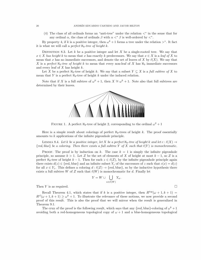
Note that if X is a full subtree of ωk + 1, then X ∼= ωk + 1. Note also that full subtrees aredetermined by their leaves.
Figure 1. A perfect ℵ0-tree of height 2, corresponding to the ordinal ω2 + 1
Here is a simple result about colorings of perfect ℵ0-trees of height k. The proof essentiallyamounts to k applications of the infinite pigeonhole principle.
Lemma 8.4. Let k be a positive integer, let X be a perfect ℵ0-tree of height k and let c : `(X)→{red, blue} be a coloring. Then there exists a full subtree Y of X such that `(Y ) is monochromatic.
Proof. The proof is by induction on k. The case k = 1 is simply the infinite pigeonholeprinciple, so assume k > 1. Let Z be the set of elements of X of height at most k − 1, so Z is aperfect ℵ0-tree of height k − 1. Then for each z ∈ `(Z), by the infinite pigeonhole principle againthere exists d(z) ∈ {red,blue} and an infinite subset Yz of the successors of z such that c(x) = d(z)for all x ∈ Yz. This defines a coloring d : `(Z) → {red,blue}, so by the inductive hypothesis thereexists a full subtree W of Z such that `(W ) is monochromatic for d. Finally let
Y = W ∪⋃
w∈`(W )
Yw.
Then Y is as required. �
Recall Theorem 4.1, which states that if k is a positive integer, then Rtop(ω + 1, k + 1) =Rcl(ω + 1, k + 1) ≥ ωk + 1. To illustrate the relevance of these notions, we now provide a secondproof of this result. This is also the proof that we will mirror when the result is generalized inTheorem 9.1.
The crux of the proof is the following result, which says that any {red,blue}-coloring of ωk + 1avoiding both a red-homogeneous topological copy of ω + 1 and a blue-homogeneous topological

TOPOLOGICAL RAMSEY NUMBERS 21
copy of ω is in some sense similar to the k+1-partite {red,blue}-coloring that falls out of the proofsof Propositions 3.1 and 3.4.
Lemma 8.5. Let k be a positive integer and let c : [ωk+1]2 → {red, blue} be a coloring. Supposethat
(a) there is no red-homogeneous topological copy of ω + 1, and(b) there is no blue-homogeneous topological copy of ω.
Under these assumptions, there is a full subtree X of ωk + 1 such that for all x, y, z ∈ X:
(1) if xC∗ z and y C∗ z then c({x, y}) = red; and(2) if x <∗ y then c({x, y}) = blue.
The proof makes use of Lemma 8.4.
Proof. The proof is by induction on k.For the base case, suppose k = 1. By the infinite Ramsey theorem there exists an infinite
homogeneous subset Y ⊆ ω. By condition (b) this must be red-homogeneous. Now by the infinitepigeonhole principle there must exist i ∈ {red,blue} and an infinite subset Z ⊆ Y such thatc({x, ω}) = i for all x ∈ Z. By condition (a) we must have i = blue. Then Z ∪{ω} is a full subtreeof ω + 1 with the required properties.
For the inductive step, suppose k > 1. First apply the inductive hypothesis to obtain a fullsubtree Ym of
[ωk ·m+ 1, ωk · (m+ 1)
] ∼= ωk−1 + 1 for each m ∈ ω, and let Y =⋃m∈ω Ym ∪ {ωk}.
Then use the inductive hypothesis again to obtain a full subtree Z of Y \ `(Y ) ∼= ωk−1 + 1, and let
W = Z ∪ {y ∈ `(Y ) | y C∗ z for some z ∈ Z}.By our uses of the inductive hypothesis, conditions (1) and (2) hold whenever x, y, z ∈ Ym for somem ∈ ω or x, y, z ∈ Z. Thus it is sufficient to find a full subtree X of W such that c({x, ωk}) = bluefor all x ∈ `(X). To do this, define a coloring c : `(W ) → {red,blue} by c(x) = c({x, ωk}). Thenapply Lemma 8.4 to obtain i ∈ {red,blue} and a full subtree X of W such that c({x, ωk}) = ifor all x ∈ `(X). Now let V be a cofinal subset of `(X) of order type ω. By the infinite Ramseytheorem there exists an infinite homogeneous subset U ⊆ V , which by condition (b) must be red-homogeneous. But then U ∪ {ωk} is a topological copy of ω + 1, so by condition (a) we must havei = blue, and we are done. �
Theorem 4.1 now follows easily.
Second proof of Theorem 4.1. As in the first proof, Rtop(ω+1, k+1) = Rcl(ω+1, k+1) ≥ωk + 1.
To see that ωk + 1→top (ω + 1, k+ 1)2, let c : [ωk + 1]2 → {red,blue} be a coloring. If there isa red-homogeneous topological copy of ω+ 1 or a blue-homogeneous topological copy of ω, then weare done. Otherwise, choose X ⊆ ωk + 1 as in Lemma 8.5. Then any branch (i.e., maximal chainunder >∗) of X forms a blue-homogeneous set of k + 1 points. �
We conclude this section by proving our bounds on Rtop(ω · 2, 3). Before doing this, we remarkthat it is crucial that we consider here the topological rather than the closed Ramsey number. Sinceω+n ∼= ω+1 for every positive integer n, from a topological perspective, ω ·2 is the simplest ordinalspace larger than ω + 1. Moreover, there are sets of ordinals containing a topological copy of ω · 2but not even a closed copy of ω+2, such as (ω ·2+1)\{ω}. Accordingly, we have only been able toapply the technique we present here to this simplest of cases. Nonetheless, it may still be possibleto adapt this technique to obtain upper bounds on closed (as well as topological) Ramsey numbers.
22 ANDRES EDUARDO CAICEDO AND JACOB HILTON
We begin by proving the lower bound. Recall from Fact 3.3 that P top(ω · 2)2 = ω2 · 2. Thus wehave indeed improved upon the lower bound given by Proposition 3.1. As with the lower bound ofLemma 5.3, we provide a simple coloring based on a small finite graph.
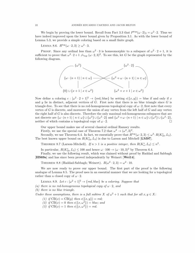
Lemma 8.6. Rtop(ω · 2, 3) ≥ ω2 · 3.
Proof. Since any ordinal less than ω2 · 3 is homeomorphic to a subspace of ω2 · 2 + 1, it issufficient to prove that ω2 · 2 + 1 6→top (ω · 2, 3)2. To see this, let G be the graph represented by thefollowing diagram.
{0} ∪ {x+ 1 | x ∈ ω2}
{ω · (n+ 1) | n ∈ ω}
{ω2}
{ω2 + x+ 1 | x ∈ ω2}
{ω2 + ω · (n+ 1) | n ∈ ω}
{ω2 · 2}
Now define a coloring c : [ω2 · 2 + 1]2 → {red,blue} by setting c({x, y}) = blue if and only if xand y lie in distinct, adjacent vertices of G. First note that there is no blue triangle since G istriangle-free. To see that there is no red-homogeneous topological copy of ω ·2, first note that everyvertex of G is discrete, and moreover the union of any vertex from the left half of G and any vertexthe right half of G is also discrete. Therefore the only maximal red-homogeneous subspaces that arenot discrete are {ω · (n+ 1) | n ∈ ω}∪{ω2}∪{ω2 ·2} and {ω2 +ω · (n+ 1) | n ∈ ω}∪{ω2}∪{ω2 ·2},neither of which contains a topological copy of ω · 2. �
Our upper bound makes use of several classical ordinal Ramsey results.Firstly, we use the special case of Theorem 7.2 that ω2 → (ω2, 3)2.Secondly, we use Theorem 6.4. In fact, we essentially prove that Rtop(ω ·2, 3) ≤ ω3 ·R(K∗10, L3).
The best known upper bound on R(K∗10, L3) is due to Larson and Mitchell [LM97].
Theorem 8.7 (Larson-Mitchell). If n > 1 is a positive integer, then R(K∗n, L3) ≤ n2.
In particular, R(K∗10, L3) ≤ 100 and hence ω · 100→ (ω · 10, 3)2 by Theorem 6.4.Finally, we use the following result, which was claimed without proof by Haddad and Sabbagh
[HS69a] and has since been proved independently by Weinert [Wei14].
Theorem 8.8 (Haddad-Sabbagh; Weinert). R(ω2 · 2, 3) = ω2 · 10.
We are now ready to prove our upper bound. The first part of the proof is the followinganalogue of Lemma 8.5. The proof uses in an essential manner that we are looking for a topologicalrather than a closed copy of ω · 2.
Lemma 8.9. Let c : [ω2 + 1]2 → {red, blue} be a coloring. Suppose that
(a) there is no red-homogeneous topological copy of ω · 2, and(b) there is no blue triangle.
Under these assumptions, there is a full subtree X of ω2 + 1 such that for all x, y ∈ X:
(1) if CB(x) = CB(y) then c({x, y}) = red;(2) if CB(x) = 0 then c({x, ω2}) = blue; and(3) if CB(x) = 1 then c({x, ω2}) = red.
TOPOLOGICAL RAMSEY NUMBERS 23
Proof. First note that (ω2 + 1) \ (ω2 + 1)′ has order type ω2, so by condition (b) it has ared-homogeneous subset W of order type ω2, since ω2 → (ω2, 3)2. Let Y0 be a full subtree of ω2 + 1
with `(Y0) ⊆ W . By applying the infinite Ramsey theorem to Y ′0 \ Y(2)0 , we may similarly pass to
a full subtree Y1 of Y0 such that Y ′1 \ Y(2)1 is red-homogeneous. Thus Y1 satisfies condition (1).
Next apply Lemma 8.4 to obtain i ∈ {red,blue} and a full subtree Z of Y1 such that c({x, ω2}) =i for all x ∈ `(Z). If i = red, then `(Z) ∪ {ω2} would be red-homogeneous, so by condition (a),i = blue and Z satisfies condition (2).
Finally apply the infinite pigeonhole principle to Z ′ \ Z(2) to obtain j ∈ {red,blue} and afull subtree X of Z such that c({x, ω2}) = j for all x ∈ X with CB(x) = 1. If j = blue, then bycondition (b) we would have c({x, y}) = red for all x, y ∈ X with CB(x) = 0 and CB(y) = 1, whenceX \ {ω2} would be red-homogeneous. Hence by condition (a), j = red and X is as required. �
We can now complete the proof of our upper bound and hence of Theorem 8.1.
Proof of Theorem 8.1. By Lemma 8.6, it remains only to prove that Rtop(ω·2, 3) ≤ ω3 ·100.Let X = ω3 · 100, let c : [X]2 → {red,blue} be a coloring and suppose by contradiction that
there is no red-homogeneous topological copy of ω · 2 and no blue triangle.First note that X(2) \ X(3) has order type ω · 100, so it has a red-homogeneous subset U of
order type ω · 10, since ω · 100→ (ω · 10, 3)2. Next let V = {x ∈ X | xC∗ y for some y ∈ U}. Notethat V has order type ω2 · 10, and so V has a red-homogeneous subset W of order type ω2 · 2, sinceω2 · 10→ (ω2 · 2, 3)2 by Theorem 8.8. Finally, let
Y = cl(W ) ∪ {x ∈ X | xC∗ y for some y ∈W},
where cl denotes the topological closure operation. Replacing Y with Y \ {maxY } if necessary,we may then assume that Y ∼= ω3 · 2, and by construction both Y (2) \ Y (3) and Y ′ \ Y (2) arered-homogeneous.
Assume for notational convenience that Y = ω3 · 2. By applying Lemma 8.9 to the interval[ω2 · α+ 1, ω2 · (α+ 1)
]for each α ∈ ω · 2, we may assume that
c({ω2 · α+ ω · (n+ 1), ω2 · (α+ 1)}) = red
for all n ∈ ω. By applying Lemma 8.9 to (ω3+1)′, we may then assume that c({ω2·(α+1), ω3}) = redand c({ω2 · α+ ω · (n+ 1), ω3}) = blue for all α, n ∈ ω.
Finally by applying the infinite pigeonhole principle to {ω2 · (α + 1) | α ∈ [ω, ω · 2)}, we mayassume that
c({ω3, ω2 · (α+ 1)}) = i
for all α ∈ [ω, ω · 2), where i ∈ {red,blue}, and then by applying the infinite pigeonhole principleto {ω · (n+ 1) | n ∈ ω}, we may assume that
c({ω · (n+ 1), ω3 + ω2}) = j,
where j ∈ {red,blue}. Now if i = red, then (ω3 ·2)(2) would be a red-homogeneous topological copyof ω · 2, and if j = red, then
{ω · (n+ 1) | n ∈ ω} ∪ {ω3 + ω · (n+ 1) | n ∈ ω} ∪ {ω3 + ω2}
would be a red-homogeneous topological copy of ω · 2. So i = j = blue. But then {ω, ω3, ω3 + ω2}is a blue triangle. �
24 ANDRES EDUARDO CAICEDO AND JACOB HILTON
Remark 8.10. Contrast this upper bound with Rcl(ω · 2, 3) ≤ ω4 · 2 (see Proposition 6.6).Very recently, Omer Mermelstein has produced a draft [Mer17] where, using a careful topologicalanalysis building in part on the ideas from this section, he obtains that Rcl(ω · 2, 3) = ω3 · 2, inparticular improving our upper bounds in both the topological and the closed case.
9. The ordinal ω2 + 1
We now use our earlier result on ω2 together with some of the ideas from the previous sectionto obtain upper bounds for ω2 + 1. We deduce these from Theorem 7.1 and the following generalresult.
Theorem 9.1. Let α and β be countable ordinals with β > 0, let k be a positive integer, andsuppose they satisfy a “cofinal version” of
ωωα
→cl (ωβ , k + 2)2.
Then
ωωα·(k+1) + 1→cl (ωβ + 1, k + 2)2.
Moreover, if ωωα
> ωβ, then in fact
ωωα·k + 1→cl (ωβ + 1, k + 2)2.
The cofinal version of the partition relation requires that for every coloring c :[ωω
α]2 → {red, blue},• there is a blue-homogeneous set of k + 2 points, or• there is a red-homogeneous closed copy of ωβ that is cofinal in ωω
α
, or• there is already a red-homogeneous closed copy of ωβ + 1.
Before providing the proof, we first deduce our upper bounds for ω2 + 1. Since ω2 + 1 isorder-reinforcing, it follows that Rtop(ω2 + 1, k + 2) = Rcl(ω2 + 1, k + 2) ≤ ωω·k + 1.
Corollary 9.2. If k is a positive integer, then ωω·k + 1→cl (ω2 + 1, k + 2)2.
Proof. By Theorem 9.1, since ωω > ω2 it is enough to prove the cofinal version of ωω →cl
(ω2, k + 2)2. The usual version is precisely Theorem 7.1, and the cofinal version is easily obtainedfrom the same proof, as indicated in Remark 7.3. �
Observe that by applying Ramsey’s theorem instead of Theorem 7.1, one obtains yet anotherproof of Theorem 4.1 from the case α = 0. Indeed, our proof of Theorem 9.1 is similar to oursecond proof of that result, though we do not explicitly use any of our results on the anti-treepartial ordering.
The bulk of the proof of Theorem 9.1 is in the following result, which is our analogue of Lemma8.5. The proof makes detailed use of the topological structure of countable ordinals. In particular,we use two arguments due to Weiss from the proof of [Bau86, Theorem 2.3]. It may be helpful forthe reader to first study that proof.
Lemma 9.3. Let α, β and k be as in Theorem 9.1. Let l be a positive integer and let c :[ωω
α·l + 1]2 → {red, blue} be a coloring. Suppose that
(1) there is no red-homogeneous closed copy of ωβ + 1, and(2) there is no blue-homogeneous set of k + 2 points.
Under these assumptions, there exists a cofinal subset X ⊆ ωωα·l such that X is a closed copy of
ωωα·l and c({x, ωωα·l}) = blue for all x ∈ X.

TOPOLOGICAL RAMSEY NUMBERS 25
Proof. The proof is by induction on l.For the case l = 1, since ωω
α →cl (ωωα
)12, there exists X ⊆ ωω
α
and i ∈ {red,blue} such thatX is a closed copy of ωω
α
(and therefore X is cofinal in ωωα
) and c({x, ωωα}) = i for all x ∈ X.Suppose for contradiction that i = red. By our assumptions together with the definition of thecofinal version of the partition relation, there exists a cofinal subset Y ⊆ X such that Y is a closedcopy of ωβ and [Y ]2 ⊆ c−1({red}). But then Y ∪{ωωα} is a red-homogeneous closed copy of ωβ +1,contrary to assumption 1. Hence i = blue and we are done.
For the inductive step, suppose l > 1. Let
Z ={ωω
α
· γ | γ ∈ ωωα·(l−1) \ {0}
},
so Z is a closed copy of ωωα·(l−1). By the inductive hypothesis, there exists a cofinal subset
Y ⊆ Z such that Y is a closed copy of ωωα·(l−1) and c({x, ωωα·l}) = blue for all x ∈ Y . Write
Y = {yδ | δ ∈ ωωα·(l−1)} in increasing order. Then by Weiss’s lemma [Bau86, Lemma 2.6], for
each δ ∈ ωωα·(l−1) there exists a cofinal subset Zδ ⊆ (yδ, yδ+1) such that Zδ is a closed copy of ωωα
.Now since ωω
α →cl (ωωα
)12, for each δ ∈ ωωα·(l−1) there exists Xδ ⊆ Zδ and iδ ∈ {red,blue}
such that Xδ is a closed copy of ωωα
(and therefore Xδ is cofinal in Zδ) and c({x, ωωα·l}) = iδ forall x ∈ Xδ. Recall now that ωω
α·(l−1) → (ωωα·(l−1))1
2 since ωωα·(l−1) is a power of ω. It follows that
there exists S ⊆ ωωα·(l−1) of order type ωωα·(l−1) and i ∈ {red,blue} such that iδ = i for all δ ∈ S.
Suppose for contradiction that i = red. We now use an argument from the proof of [Bau86,Theorem 2.3]. Let (δm)m∈ω be a strictly increasing cofinal sequence from S, and let (ηm)m∈ω bea strictly increasing cofinal sequence from ωα (or let ηm = 0 for all m ∈ ω if α = 0). For eachm ∈ ω, pick Wm ⊆ Xδm such that Wm is a closed copy of ωηm + 1, and let W =
⋃m∈ωWm. Note
that W is cofinal in ωωα·l, W is a closed copy of ωω
α
and c({x, ωωα·l}) = red for all x ∈ W . Byour assumptions together with the definition of the cofinal version of the partition relation, thereexists a cofinal subset V ⊆W such that V is a closed copy of ωβ and [V ]2 ⊆ c−1({red}). But thenV ∪ {ωωα·l} is a red-homogeneous closed copy of ωβ + 1, contrary to assumption 1.
Therefore i = blue. Finally, let
X =⋃δ∈S
Xδ ∪ cl({yδ+1 | δ ∈ S}),
where cl denotes the topological closure operation. Then the set X is as required. �
We may now deduce Theorem 9.1 in the much same way that we deduced Theorem 4.1 fromLemma 8.5.
Proof of Theorem 9.1. First assume that ωωα
> ωβ . We prove by induction on l that forall l ∈ {1, 2, . . . , k},
ωωα·l + 1→cl (ωβ + 1, l + 2)2.
In every case, if either of the assumptions in Lemma 9.3 does not hold, then we are done sincel ≤ k. We may therefore choose X as in Lemma 9.3.
For the base case l = 1, to avoid a blue triangle, X must be red-homogeneous. But X containsa closed copy of ωβ + 1 since ωω
α ≥ ωβ + 1, and so we are done.For the inductive step, suppose l ≥ 2. Then X has a closed copy Y of ωω
α·(l−1) + 1. By theinductive hypothesis, either Y contains a red-homogeneous closed copy of ωβ + 1, in which case weare done, or Y contains a blue-homogeneous set Z of l + 1 points. But in that case Z ∪ {ωωα·l} isa blue-homogeneous set of l + 2 points, and we are done.

26 ANDRES EDUARDO CAICEDO AND JACOB HILTON
Finally, if we cannot assume that ωωα
> ωβ , then the base case breaks down. However, wemay instead use the base case ωω
α
+ 1→cl (ωβ + 1, 2)2, which follows from the fact that ωωα ≥ ωβ .
The inductive step is then identical. �
10. The weak topological Erdos-Milner theorem
Finally we reach our main result, which demonstrates that Rtop(α, k) and Rcl(α, k) are count-able for all countable α and all finite k.
This is a topological version of a classical result due to Erdos and Milner [EM72]. Beforestating it, we first provide a simplified proof of the classical version.
Theorem 10.1 (Weak Erdos-Milner). Let α and β be countable nonzero ordinals, and let k > 1be a positive integer. If
ωα → (ω1+β , k)2,
thenωα+β → (ω1+β , k + 1)2.
Since trivially ω1+α → (ω1+α, 2)2, it follows by induction on k that R(ω1+α, k + 1) ≤ ω1+α·k
for all countable α and finite k. In fact, Erdos and Milner proved a stronger version of the abovetheorem, in which k+ 1 is replaced by 2k, implying that R(ω1+α, 2k) ≤ ω1+α·k. This is why we usethe adjective weak here.
Our proof is essentially a simplified version of the original, which can be found in [Wil77,Theorem 7.2.10]. The basic idea is to write ωα+β as a sequence of ωβ intervals, each of order typeωα, to list these intervals in type ω, and to recursively build up a red-homogeneous copy of ωβ
consisting of one element from each interval. This would achieve the above theorem with 1 + βweakened to β. To obtain a copy of ω1+β , we simply choose infinitely many elements from eachinterval instead of just one. In the proof we use the fact that ωα → (ωα)1
m for all finite m.
Proof. Let c :[ωα+β
]2 → {red,blue} be a coloring.
For each x ∈ ωβ , letIx = [ωα · x, ωα · (x+ 1)) ,
so Ix has order type ωα. Let (xn)n∈ω be a sequence of points from ωβ in which every memberof ωβ appears infinitely many times. We attempt to inductively build a red-homogeneous setA = {an | n ∈ ω} of order-type ω1+β with an ∈ Ixn for every n ∈ ω.
Suppose that we have chosen a1, a2, . . . , am−1 for some m ∈ ω. Let
P = {an | n ∈ {1, 2, . . . ,m− 1}, an ∈ Ixm},and let
J =
{Ixm , if P = ∅Ixm \ [0,maxP ], if P 6= ∅,
so J has order type ωα. For each n ∈ {1, 2, . . . ,m− 1} let
Jn = {a ∈ J | c({an, a}) = blue}.
If⋃m−1n=1 Jn = J , then since ωα → (ωα)1
m−1, Jn has order type ωα for some n ∈ {1, 2, . . . ,m − 1}.Then since ωα → (ω1+β , k)2, Jn either has a red-homogeneous subset of order type ω1+β , in whichcase we are done, or a blue-homogeneous subset B of k points, in which case B ∪ {an} is a blue-
homogeneous set of k + 1 points, and we are done. Thus we may assume that J \⋃m−1n=1 Jn 6= ∅,
and choose am to be any member of this set.

TOPOLOGICAL RAMSEY NUMBERS 27
Clearly the resulting set A is red-homogeneous. To see that it has order type ω1+β , simplyobserve that by choice of (xn)n∈ω, A ∩ Ix is infinite for all x ∈ ωβ , and that by choice of J , A ∩ Ixin fact has order type ω for all x ∈ ωβ . �
Here is our topological version of the weak Erdos-Milner theorem.
Theorem 10.2 (The weak topological Erdos-Milner theorem). Let α and β be countable nonzeroordinals, and let k > 1 be a positive integer. If
ωωα
→top (ωβ , k)2,
then
ωωα·β →top (ωβ , k + 1)2.
In particular, as we shall deduce in Corollary 10.5, Rtop(α, k) and Rcl(α, k) are countablewhenever α is a countable ordinal and k is a positive integer.
Our proof follows the same outline as our proof of the classical version, except that we useintervals in the sense of the anti-tree partial ordering rather than in the usual sense. Furthermore,rather than constructing a closed copy of ωβ directly, we instead construct a larger set and thenthin it out. As in the previous section, we make detailed use of the structure of countable ordinals,including an argument from the proof of [Bau86, Lemma 2.6]. Note that the proof does not directlyuse any of our previous results.
Proof. Let c :[ωω
α·β]2 → {red,blue} be a coloring.
First of all, fix a strictly increasing cofinal sequence (γn)n∈ω from ωωα
.Define an indexing set of pairs
S ={
(x, y) | x ∈ β, ωωα·(x+1) · y ∈ ωω
α·β},
and for each (x, y) ∈ S, let
X(x,y) ={ωω
α·(x+1) · y + ωωα·x · z | z ∈ ωω
α
\ {0}},
so X(x,y) is a closed copy of ωωα
. Let (xn, yn)n∈ω be a sequence of pairs from S in which everymember of S appears infinitely many times. We attempt to inductively build a red-homogeneousset A = {an | n ∈ ω}, which will contain a closed copy of ωβ , with an ∈ X(xn,yn) for every n ∈ ω.
Suppose that we have chosen a1, a2, . . . , am−1 for some m ∈ ω. Let
P ={an | n ∈ {1, 2, . . . ,m− 1}, an ∈ X(xm,ym)
},
let
Q = P ∪{ωω
α·(xm+1) · ym + ωωα·xm · γ|P |
},
and let
Y = X(xm,ym) \ [0,maxQ],
so Y is a closed copy of ωωα
. For each n ∈ {1, 2, . . . ,m− 1} let
Yn = {a ∈ Y | c({an, a}) = 1}.
If⋃m−1n=1 Yn = Y , then since ωω
α →cl (ωωα
)1m−1, Yn contains a closed copy of ωω
α
for some
n ∈ {1, 2, . . . ,m − 1}. Then since ωωα →cl (ωβ , k)2, Yn either contains a red-homogeneous closed
copy of ωβ , in which case we are done, or a blue-homogeneous set B of k points, in which case

28 ANDRES EDUARDO CAICEDO AND JACOB HILTON
B ∪ {an} is a blue-homogeneous set of k + 1 points, and we are done. Thus we may assume that
Y \⋃m−1n=1 Yn 6= ∅, and choose am to be any member of this set.
Clearly the resulting set A is red-homogeneous. To complete the proof, observe that by choiceof (xn, yn)n∈ω, A∩X(x,y) is infinite for all (x, y) ∈ S, and that by choice of Q, A∩X(x,y) is a cofinalsubset of X(x,y) of order type ω for all (x, y) ∈ S. We claim that this property is enough to ensure
that A contains a closed copy of ωβ .To prove the claim, for each δ ∈ [1, β] and each ordinal y with ωω
α·δ · y ∈ ωωα·β we find a
cofinal subset Cδ,y ⊆[ωω
α·δ · y + 1, ωωα·δ · (y + 1)
)such that Cδ,y ⊆ A and Cδ,y is a closed copy of
ωδ; then Cβ,0 ⊆ A is a closed copy of ωβ , as required. We do this by induction on δ.
First suppose δ ∈ [1, β] is a successor ordinal, say δ = x+ 1. Fix an ordinal y with ωωα·δ · y ∈
ωωα·β , and observe that (x, y) ∈ S and that X(x,y) is a cofinal subset of the interval[
ωωα·δ · y + 1, ωω
α·δ · (y + 1)).
Recall now that A ∩ X(x,y) is a cofinal subset of X(x,y) of order type ω. Thus if δ = 1 then wemay simply take C1,y = A ∩ X(0,y), so assume δ > 1, and write A ∩ X(x,y) = {bn | n ∈ ω} inincreasing order. For each n ∈ ω \ {0} we find a cofinal subset Dn ⊆ (bn−1, bn) such that Dn ⊆ Aand Dn is a closed copy of ωx; then we may take Cδ,y =
⋃n∈ω\{0}Dn ∪ {bn}. We do this using
an argument essentially taken from the proof of [Bau86, Lemma 2.6]. Fix n ∈ ω \ {0} and writebn = ωω
α·(x+1) · y+ωωα·x · z with z ∈ ωωα \ {0}. Let v = ωω
α · y+ z so that bn = ωωα·x · v. If v is a
successor ordinal, say v = u+ 1, then by the inductive hypothesis we may take Dn = Cx,u. If v is a
limit ordinal, then let (um)m∈ω be a strictly increasing cofinal sequence from v with ωωα·x ·u0 ≥ bn−1
and let (ηm)m∈ω be a strictly increasing cofinal sequence from ωx. By the inductive hypothesis, foreach m ∈ ω we may choose a subset Em ⊆ Cx,um such that Em is a closed copy of ηm + 1. Thentake Dn =
⋃m∈ω Em.
Suppose instead δ ∈ [1, β] is a limit ordinal. Fix an ordinal y with ωωα·δ · y ∈ ωω
α·β . Let(xn)n∈ω be a strictly increasing cofinal sequence from δ. For each n ∈ ω, let ζn be the ordinal suchthat δ = xn + 1 + ζn and let yn = ωω
α·ζn · y + 1. Then ωωα·(xn+1) · yn = ωω
α·δ · y + ωωα·(xn+1) and
so Cxn+1,yn ⊆[ωω
α·δ · y + ωωα·(xn+1) + 1, ωω
α·δ · y + ωωα·(xn+1) · 2
). By the inductive hypothesis,
for each n ∈ ω we may choose a subset Dn ⊆ Cxn+1,yn such that Dn is a closed copy of ωxn + 1.Then take Cδ,y =
⋃n∈ωDn. �
Remark 10.3. We expect that as in the original Erdos-Milner theorem, it should be possibleto improve k+ 1 to 2k in Theorem 10.2. Indeed, the basic argument from [Wil77, Theorem 7.2.10]works in the topological setting. The key technical difficulty appears to be in formulating andproving an appropriate topological version of statement (1) in that account.
The weak topological Erdos-Milner theorem allows us to obtain upper bounds for countableindecomposable ordinals. Before describing some of these, we first observe that by very slightlyadapting our argument, we may obtain improved bounds for other ordinals. Here is a version forordinals of the form ωβ ·m+ 1.
Theorem 10.4. Let α and β be countable nonzero ordinals, and let k > 1 be a positive integer.If
ωωα
→cl (ωβ ·m+ 1, k)2,
then
ωωα·β ·R(m, k + 1) + 1→top (ωβ ·m+ 1, k + 1)2.
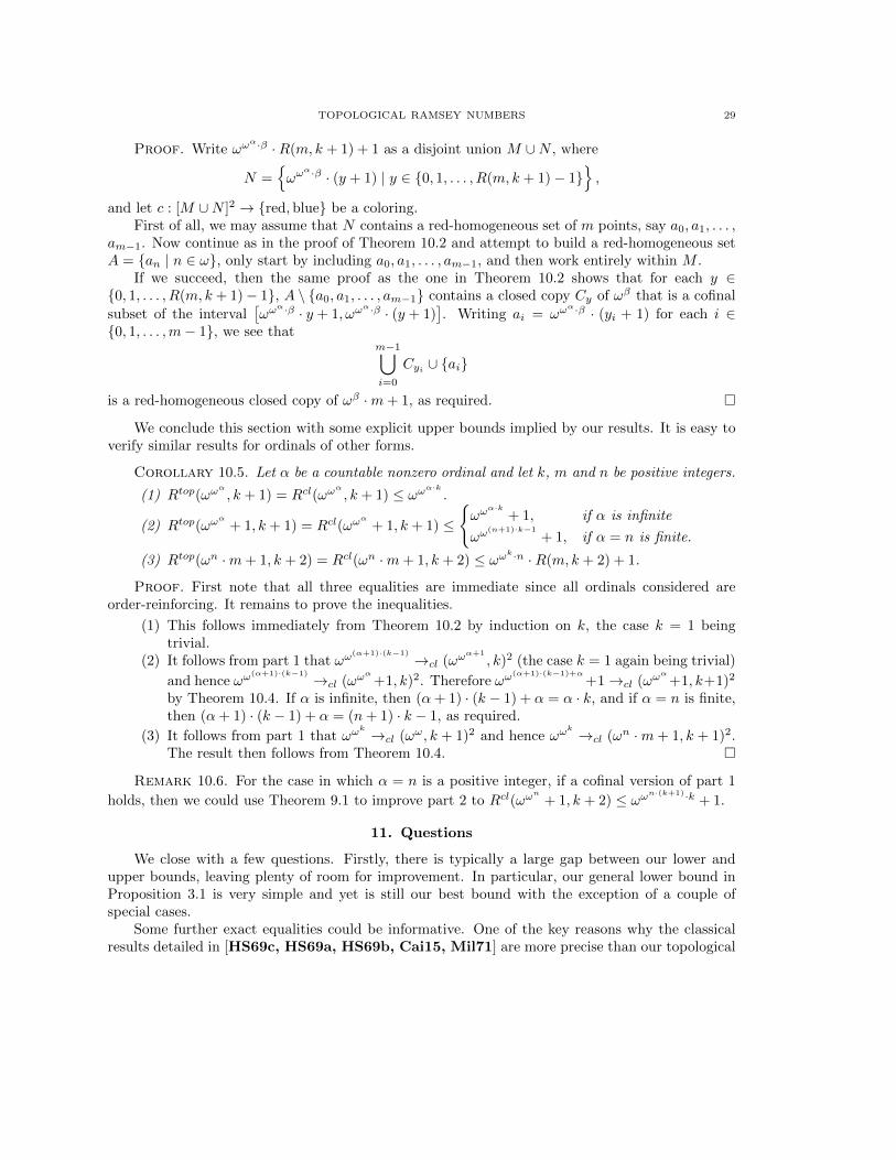
TOPOLOGICAL RAMSEY NUMBERS 29
Proof. Write ωωα·β ·R(m, k + 1) + 1 as a disjoint union M ∪N , where
N ={ωω
α·β · (y + 1) | y ∈ {0, 1, . . . , R(m, k + 1)− 1}},
and let c : [M ∪N ]2 → {red,blue} be a coloring.First of all, we may assume that N contains a red-homogeneous set of m points, say a0, a1, . . . ,
am−1. Now continue as in the proof of Theorem 10.2 and attempt to build a red-homogeneous setA = {an | n ∈ ω}, only start by including a0, a1, . . . , am−1, and then work entirely within M .
If we succeed, then the same proof as the one in Theorem 10.2 shows that for each y ∈{0, 1, . . . , R(m, k + 1)− 1}, A \ {a0, a1, . . . , am−1} contains a closed copy Cy of ωβ that is a cofinal
subset of the interval[ωω
α·β · y + 1, ωωα·β · (y + 1)
]. Writing ai = ωω
α·β · (yi + 1) for each i ∈{0, 1, . . . ,m− 1}, we see that
m−1⋃i=0
Cyi ∪ {ai}
is a red-homogeneous closed copy of ωβ ·m+ 1, as required. �
We conclude this section with some explicit upper bounds implied by our results. It is easy toverify similar results for ordinals of other forms.
Corollary 10.5. Let α be a countable nonzero ordinal and let k, m and n be positive integers.
(1) Rtop(ωωα
, k + 1) = Rcl(ωωα
, k + 1) ≤ ωωα·k.
(2) Rtop(ωωα
+ 1, k + 1) = Rcl(ωωα
+ 1, k + 1) ≤
{ωω
α·k+ 1, if α is infinite
ωω(n+1)·k−1
+ 1, if α = n is finite.
(3) Rtop(ωn ·m+ 1, k + 2) = Rcl(ωn ·m+ 1, k + 2) ≤ ωωk·n ·R(m, k + 2) + 1.
Proof. First note that all three equalities are immediate since all ordinals considered areorder-reinforcing. It remains to prove the inequalities.
(1) This follows immediately from Theorem 10.2 by induction on k, the case k = 1 beingtrivial.
(2) It follows from part 1 that ωω(α+1)·(k−1) →cl (ωω
α+1
, k)2 (the case k = 1 again being trivial)
and hence ωω(α+1)·(k−1) →cl (ωω
α
+1, k)2. Therefore ωω(α+1)·(k−1)+α
+1→cl (ωωα
+1, k+1)2
by Theorem 10.4. If α is infinite, then (α+ 1) · (k − 1) + α = α · k, and if α = n is finite,then (α+ 1) · (k − 1) + α = (n+ 1) · k − 1, as required.
(3) It follows from part 1 that ωωk →cl (ωω, k + 1)2 and hence ωω
k →cl (ωn ·m+ 1, k + 1)2.The result then follows from Theorem 10.4. �
Remark 10.6. For the case in which α = n is a positive integer, if a cofinal version of part 1
holds, then we could use Theorem 9.1 to improve part 2 to Rcl(ωωn
+ 1, k + 2) ≤ ωωn·(k+1)·k + 1.
11. Questions
We close with a few questions. Firstly, there is typically a large gap between our lower andupper bounds, leaving plenty of room for improvement. In particular, our general lower bound inProposition 3.1 is very simple and yet is still our best bound with the exception of a couple ofspecial cases.
Some further exact equalities could be informative. One of the key reasons why the classicalresults detailed in [HS69c, HS69a, HS69b, Cai15, Mil71] are more precise than our topological

30 ANDRES EDUARDO CAICEDO AND JACOB HILTON
results in Sections 5–9 is that for various α < ωω, the computation of R(α, k) reduces to a problemin finite combinatorics. Some hint of a topological version of this appears in the proof of the lowerbounds of Lemmas 5.3 and 8.6, though it is far from clear how to obtain an exact equality.
Question 11.1. Is it possible to reduce the computation of Rtop(α, k) or Rcl(α, k) to finitecombinatorial problems, even for α < ω2?
A partition ordinal is an ordinal α satisfying α → (α, 3)2. As we have seen, ω and ω2 are
partition ordinals. Other than these, every countable partition ordinal has the form ωωβ
, and in
the other direction, ωωβ
is a partition ordinal if β has the form ωγ or ωγ + ωδ [Sch10].
Question 11.2. Are there any countable “topological partition” ordinals, satisfying α →top
(α, 3)2, other than ω?
By our lower bound (Proposition 3.1), these must all have the form ωωβ
. Since every powerof ω is order-reinforcing, this question is equivalent to the version resulting from replacing thetopological partition relation by the closed partition relation.
We expect that a strong version of the topological Erdos-Milner theorem should hold, that is,we expect that in Theorem 10.2 it should be possible to improve k + 1 to 2k.
Question 11.3. Let α and β be countable nonzero ordinals, and let k > 1 be a positive integer.Is it the case that if
ωωα
→top (ω1+β , k)2,
then
ωωα·β →top (ω1+β , 2k)2?
See Remark 10.3 for further details.Finally, it would be nice to determine whether the existing conjecture ω1 → (α, k)3 holds, and
also to discover something about the topological or closed version of this relation.
Question 11.4. Is it the case that for all countable ordinals α and all finite k, ω1 →top (α, k)3?
Again, since every power of ω is order-reinforcing, this question is equivalent if we replace thetopological partition relation by the closed partition relation. If the answer to this question is yes,then the classical and closed relations are in fact equivalent whenever the ordinal on the left-handside is ω1 and the ordinals on the right-hand side are countable.
References
[Bau86] James E. Baumgartner. Partition relations for countable topological spaces. J. Combin. Theory Ser. A,43(2):178–195, 1986. 2, 3, 4, 5, 6, 10, 24, 25, 27, 28
[Cai14] Andres E. Caicedo. Teorıa de Ramsey de ordinales contables muy pequenos. Submitted. Available athttps://andrescaicedo.wordpress.com/papers/, 2014. 4
[Cai15] Andres E. Caicedo. Partition calculus of small countable ordinals. A survey of results of Haddad andSabbagh. Preprint, 2015. 2, 17, 29
[EM72] Paul Erdos and Eric C. Milner. A theorem in the partition calculus. Canad. Math. Bull., 15:501–505, 1972.2, 26
[ER53] Paul Erdos and Richard Rado. A problem on ordered sets. J. London Math. Soc., 28:426–438, 1953. 2[ER56] Paul Erdos and Richard Rado. A partition calculus in set theory. Bull. Amer. Math. Soc., 62:427–489,
1956. 2, 3, 15
[ER67] Paul Erdos and Richard Rado. Partition relations and transitivity domains of binary relations. J. London
Math. Soc., 42:624–633, 1967. 15

TOPOLOGICAL RAMSEY NUMBERS 31
[FM88] Jorg Flum and Juan Carlos Martınez. On topological spaces equivalent to ordinals. J. Symbolic Logic,53(3):785–795, 1988. 7
[Fri74] Harvey Friedman. On closed sets of ordinals. Proc. Amer. Math. Soc., 43:190–192, 1974. 3
[Haj60] Andras Hajnal. Some results and problems on set theory. Acta Math. Acad. Sci. Hungar., 11:277–298,1960. 3
[Haj64] Andras Hajnal. Remarks on the theorem of W. P. Hanf. Fund. Math., 54:109–113, 1964. 3[Hil16] Jacob Hilton. The topological pigeonhole principle for ordinals. J. Symb. Log., 81(2):662–686, 2016. 3, 4,
6, 7, 8, 9, 10, 18
[HJW90] Andras Hajnal, Istvan Juhasz, and William Weiss. Partitioning the pairs and triples of topological spaces.Topology Appl., 35(2-3):177–184, 1990. 3
[HL10] Andras Hajnal and Jean A. Larson. Partition relations. In Handbook of set theory. Vols. 1, 2, 3, pages
129–213. Springer, Dordrecht, 2010. 2[HS69a] Labib Haddad and Gabriel Sabbagh. Calcul de certains nombres de Ramsey generalises. C. R. Acad. Sci.
Paris Ser. A-B, 268:A1233–A1234, 1969. 2, 17, 18, 22, 29
[HS69b] Labib Haddad and Gabriel Sabbagh. Nouveaux resultats sur les nombres de Ramsey generalises. C. R.Acad. Sci. Paris Ser. A-B, 268:A1516–A1518, 1969. 2, 29
[HS69c] Labib Haddad and Gabriel Sabbagh. Sur une extension des nombres de Ramsey aux ordinaux. C. R. Acad.
Sci. Paris Ser. A-B, 268:A1165–A1167, 1969. 2, 17, 29[Jon00] Albin L. Jones. A short proof of a partition relation for triples. Electron. J. Combin., 7:Research Paper
24, 9, 2000. 3
[Jon17] Albin L. Jones. Even more on partitioning triples of countable ordinals. Proc. Amer. Math. Soc., 2017. Toappear. 3
[KL06] Vincent Kieftenbeld and Benedikt Lowe. A classification of ordinal topologies. Unpublished. Available athttps://www.illc.uva.nl/Research/Publications/PP-2006-57.text.pdf, 2006. 7
[Kru65] Arthur H. Kruse. A note on the partition calculus of P. Erdos and R. Rado. J. London Math. Soc.,
40:137–148, 1965. 3[Lav75] Richard J. Laver. Partition relations for uncountable cardinals ≤ 2ℵ0 . In Infinite and finite sets (Colloq.,
Keszthely, 1973; dedicated to P. Erdos on his 60th birthday), Vol. II, pages 1029–1042. Colloq. Math. Soc.
Janos Bolyai, Vol. 10. North-Holland, Amsterdam, 1975. 3[LM97] Jean A. Larson and William J. Mitchell. On a problem of Erdos and Rado. Ann. Comb., 1(3):245–252,
1997. 22
[Mer17] Omer Mermelstein. Calculating the closed ordinal Ramsey number Rcl(ω · 2, 3)2. Preprint. Available athttps://arxiv.org/abs/1702.03878, 2017. 24
[Mil71] Eric C. Milner. A finite algorithm for the partition calculus. In Proceedings of the Twenty-Fifth Summer
Meeting of the Canadian Mathematical Congress (Lakehead Univ., Thunder Bay, Ont., 1971), pages117–128. Lakehead Univ., Thunder Bay, Ont., 1971. 2, 29
[Pn15] Claribet Pina. A topological Ramsey classification of countable ordinals. Acta Math. Hungar., 147(2):477–
509, 2015. 5, 19[Ros15] Shai Rosenberg. Infinite closed monochromatic subsets of a metric space. Preprint. Available at
https://arxiv.org/abs/1508.02366, 2015. 3[Sch10] Rene Schipperus. Countable partition ordinals. Ann. Pure Appl. Logic, 161(10):1195–1215, 2010. 2, 30
[Sch12] Rene Schipperus. The topological Baumgartner-Hajnal theorem. Trans. Amer. Math. Soc., 364(8):3903–
3914, 2012. 3[Sie33] Waclaw Sierpinski. Sur un probleme de la theorie des relations. Ann. Scuola Norm. Sup. Pisa Cl. Sci. (2),
2(3):285–287, 1933. 2[Spe57] Ernst Specker. Teilmengen von Mengen mit Relationen. Comment. Math. Helv., 31:302–314, 1957. 2, 18[Tod83] Stevo Todorcevic. Forcing positive partition relations. Trans. Amer. Math. Soc., 280(2):703–720, 1983. 3
[Tod96] Stevo Todorcevic. A partition property of spaces with point-countable bases. Unpublished. 1 pg., June
1996. 4[Wei90] William Weiss. Partitioning topological spaces. In Mathematics of Ramsey theory, volume 5 of Algorithms
Combin., pages 154–171. Springer, Berlin, 1990. 3, 4[Wei14] Thilo V. Weinert. Idiosynchromatic poetry. Combinatorica, 34(6):707–742, 2014. 2, 22[Wil77] Neil H. Williams. Combinatorial set theory, volume 91 of Studies in Logic and the Foundations of Mathe-
matics. North-Holland Publishing Co., Amsterdam, 1977. 2, 26, 28

32 ANDRES EDUARDO CAICEDO AND JACOB HILTON
Andres Eduardo Caicedo, Boise State University, Department of Mathematics, 1910 UniversityDrive, Boise, ID 83725-1555, USA
Current address: Mathematical Reviews, 416 Fourth Street, Ann Arbor, MI 48103-4820, USA
E-mail address: [email protected]
URL: http://www-personal.umich.edu/∼caicedo/
Jacob Hilton, School of Mathematics, University of Leeds, Leeds LS2 9JT, UKE-mail address: [email protected]