Topological Properties of Skeletal · PDF fileTopological Properties ... Truss structures are...
46
CHAPTER 2 Topological Properties of Skeletal Structures 2.1 INTRODUCTION In the analysis of skeletal structures, three different properties are encountered, which can be classified as topological, geometrical and material. Separate study of these properties results in a considerable simplification in the analysis and leads to a clear understanding of the structural behaviour. This chapter is confined to partial study of the topological properties of skeletal structures, since both displacement and force methods require such a study at the beginning of the analysis. The number of equations to be solved in the two methods may differ widely for the same structure. This number depends on the size of flexibility and stiffness matrices, which are the same as the degree of statical indeterminacy (DSI) and the degree of kinematical indeterminacy (DKI) of a structure, respectively. Obviously, the method which leads to the required results with the least amount of effort, should be used for the analysis of a given structure. Thus, the comparison of the numbers of DSI and DKI may be the main deciding criterion for selecting the method of analysis. For determining the DSI and DKI of structures, numerous formulae, depending on the kinds of member or types of joint, have been given, e.g. Refs [38,200,236]. The use of these classical formulae, in general, requires counting the number of members and joints, which becomes a tedious process for multi-member and/or complex pattern structures. This counting process provides no additional information about their connectivity properties. Henderson and Bickley [77] related the DSI of a rigid-jointed frame to the first Betti number (cyclomatic number) of its graph model S. This was an important
Transcript of Topological Properties of Skeletal · PDF fileTopological Properties ... Truss structures are...
CHAPTER 2
Topological Properties of Skeletal Structures
2.1 INTRODUCTION
In the analysis of skeletal structures, three different properties are encountered, which can be classified as topological, geometrical and material. Separate study of these properties results in a considerable simplification in the analysis and leads to a clear understanding of the structural behaviour. This chapter is confined to partial study of the topological properties of skeletal structures, since both displacement and force methods require such a study at the beginning of the analysis. The number of equations to be solved in the two methods may differ widely for the same structure. This number depends on the size of flexibility and stiffness matrices, which are the same as the degree of statical indeterminacy (DSI) and the degree of kinematical indeterminacy (DKI) of a structure, respectively. Obviously, the method which leads to the required results with the least amount of effort, should be used for the analysis of a given structure. Thus, the comparison of the numbers of DSI and DKI may be the main deciding criterion for selecting the method of analysis.
For determining the DSI and DKI of structures, numerous formulae, depending on the kinds of member or types of joint, have been given, e.g. Refs [38,200,236]. The use of these classical formulae, in general, requires counting the number of members and joints, which becomes a tedious process for multi-member and/or complex pattern structures. This counting process provides no additional information about their connectivity properties.
Henderson and Bickley [77] related the DSI of a rigid-jointed frame to the first Betti number (cyclomatic number) of its graph model S. This was an important
40 Structural Mechanics: Graph and Matrix Methods
achievement, since a topological invariant of a graph was related to an essential mechanical property of the corresponding structure. Generalizing the Betti´s number to a linear function and using an expansion process, Kaveh [89] developed a general method for determining the DSI and DKI of all types of skeletal structures. Special methods have also been developed to transform the topological properties of space structures to those of their planar drawings to simplify the calculation of their DSI, Refs [90,91,109].
In this chapter, general and simple methods are presented for calculating the DSI and DKI of different types of skeletal structures, such as rigid-jointed planar and space frames, pin-jointed planar trusses and ball-jointed space trusses. Euler´s polyhedra formula is then used to develop very efficient special methods for determining the DSI of different types of structures. An automatic algorithm is presented for efficient planar embedding of structural models.
2.2 MATHEMATICAL MODEL OF A SKELETAL STRUCTURE
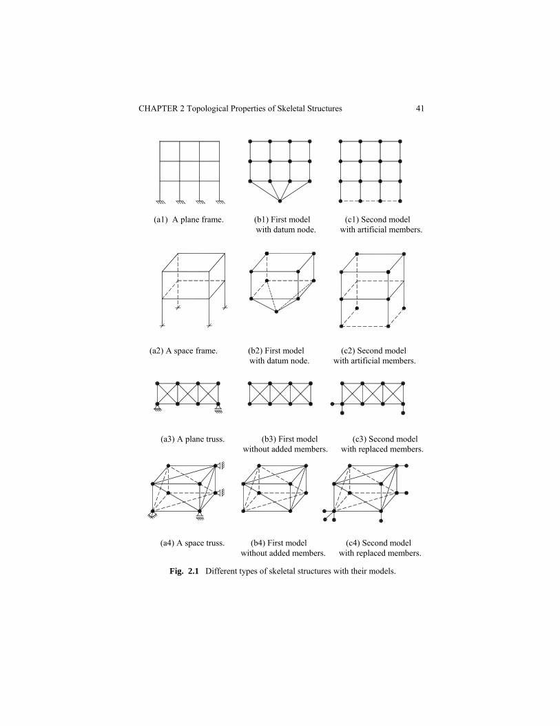
The mathematical model S of a structure is considered to be a finite, connected graph. There is a one-to-one correspondence between the elements of the structure and the members of S. There is also a one-to-one correspondence between the joints and the nodes of S, except for the support joints. Two different groups of modelling are considered. The first group is suitable for calculating the DSI and DKI of structures, and the second group is more appropriate for analysis. These models are illustrated in Figure 2.1.
For a frame structure, all the support joints are identified as a datum (ground) node in the first group of model, Figures 2.1(b1) and (b2). In the second group, all such joints are connected by an artificial tree, Figures 2.1 (c1) and (c2).
Truss structures are assumed to be supported in a statically determinate fashion (Figures 2.1 (b3) and (b4)), and the effect of additional supports can easily be included in calculating the DSI and DKI of the corresponding structures. In the second group of models, artificial members are added as shown in Figures 2.1 (c3) and (c4). For a fixed support, two members and three members are considered for planar and space trusses, respectively, and one member is used for representing a roller.
The skeletal structures are considered to be in perfect condition; i.e. planar and space trusses have pin and ball joints only. Obviously the effect of extra constraints or releases can easily be taken into account in determining their DSI and DKI, and also in their analysis, Mauch and Fenves [168].
CHAPTER 2 Topological Properties of Skeletal Structures 41
(a1) A plane frame. (b1) First model (c1) Second model with datum node. with artificial members.
(a2) A space frame. (b2) First model (c2) Second model with datum node. with artificial members.
(a3) A plane truss. (b3) First model (c3) Second model without added members. with replaced members.
(a4) A space truss. (b4) First model (c4) Second model without added members. with replaced members.
Fig. 2.1 Different types of skeletal structures with their models.
42 Structural Mechanics: Graph and Matrix Methods
2.3 UNION-INTERSECTION METHOD
The degree of kinematical indeterminacy of a structure is the number of independent displacement components (translations and rotations) required for describing a general deformation state of the structure. The DKI is also referred to as the total degrees of freedom of the structure. On the other hand, the degree of statical indeterminacy (redundancy) of a structure is the number of independent force components (forces and moments) required for describing a general equilibrium state of the structure. The DSI of a structure can be obtained by reducing the number of independent equilibrium equations from the number of its unknown forces.
Formulae for calculating the DKI and DSI of various skeletal structures can be found in text books on structural mechanics, e.g. for planar trusses each joint of which has two degrees of freedom, the DKI, denoted by η(S), is given as,
η(S) = 2N(S) − 3, (2-1)
where S is supported in a statically determinate fashion. For extra support, η(S) will further be reduced by one for each additional constraint.
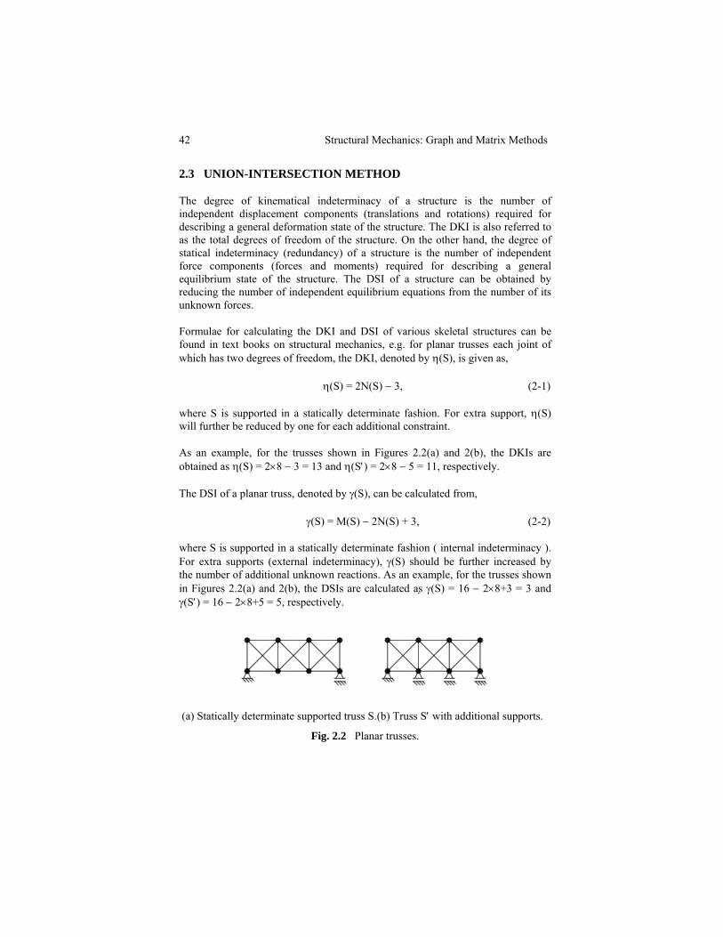
As an example, for the trusses shown in Figures 2.2(a) and 2(b), the DKIs are obtained as η(S) = 2×8 − 3 = 13 and η(S′) = 2×8 − 5 = 11, respectively.
The DSI of a planar truss, denoted by γ(S), can be calculated from,
γ(S) = M(S) − 2N(S) + 3, (2-2)
where S is supported in a statically determinate fashion ( internal indeterminacy ). For extra supports (external indeterminacy), γ(S) should be further increased by the number of additional unknown reactions. As an example, for the trusses shown in Figures 2.2(a) and 2(b), the DSIs are calculated as γ(S) = 16 − 2×8+3 = 3 and γ(S′) = 16 − 2×8+5 = 5, respectively.
(a) Statically determinate supported truss S.(b) Truss S′ with additional supports.
Fig. 2.2 Planar trusses.
CHAPTER 2 Topological Properties of Skeletal Structures 43
Similar formulae are derived for space trusses:
η(S) = 3N(S) − 6, (2-3)
γ(S) = M(S) − 3N(S) + 6. (2-4)
For the space truss of Figure 2.1(a4), these values are η(S) = 3×8 − 6 =18 and γ(S) = 18 − 3×8+6 = 0.
For planar and space frames, the classical formulae are given as,
η(S) = α[ N(S) − 1 ], (2-5)
γ(S) = α[ M(S) − N(S) + 1 ], (2-6)
where all supports are modelled as a datum (ground) node, and α = 3 or 6 for planar and space frames, respectively. As an example, η(S) and γ(S) are calculated for the planar and space frames shown in Figures 2.1(b1) and (b2). For the planar frame η(S) = 3(13 − 1) = 36 and γ(S) = 3(21 − 13+1) = 27, and for the space frame η(S) = 6(9 − 1) = 48 and γ(S) = 6(16 − 9+1) = 48.
All these formulae require counting a great number of members and nodes, which makes their application impractical for multi-member and complex pattern structures.
2.3.1 A UNIFYING FUNCTION
All the existing formulae for determining the DKI and DSI have a common property, which is their linearity with respect to M(S) and N(S). Therefore, a general unifying function is,
ν(S) = aM(S) + bN(S) + cν0(S), (2-7)
where M(S), N(S) and ν0(S) are the numbers of members, nodes and components of S, respectively. The coefficients a, b and c are integer numbers depending on both the type of the corresponding structure and the property which the function is expected to represent. For example, ν(S) with appropriate values for a, b and c may describe the DKI or DSI of certain types of skeletal structures, Table 2.1. For a = 1, b = − 1 and c = 1, ν(S) becomes the first Betti number b1(S) of S.
44 Structural Mechanics: Graph and Matrix Methods
Table 2.1 The coefficient for the classical formulae.
Type of structure ν(S) a b c
Plane frame DKI DSI
0 +3
+3 −3
−3 +3
Space frame DKI DSI
0 +6
+6 −6
−6 +6
Plane truss DKI DSI
0 +1
+2 −2
−3 +3
Space truss DKI DSI
0 +1
+3 −3
−6 +6
It should be noted the ν(S) can further be generalized to include the effect of higher order elements. As an example, when a skeletal structure contains shear panels then one may use,
ν(S) = dV(S) + aM(S) + bN(S) + cν0(S),
where V(S) is the number of shear panels of the structure, and d is an integer.
2.3.2 AN EXPANSION PROCESS
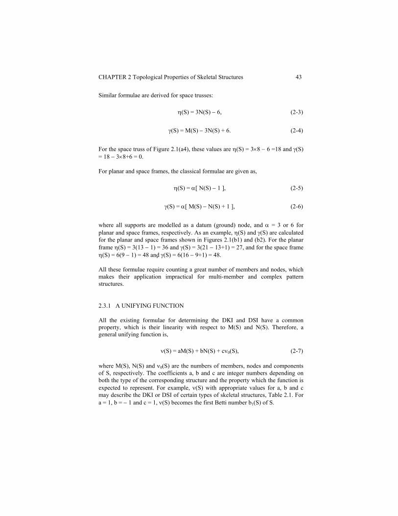
An expansion process in its simplest form has been used for re-forming structural models such as simple planar and space trusses, Müller-Breslau [176]. A simple planar truss can be formed by the following expansion process:
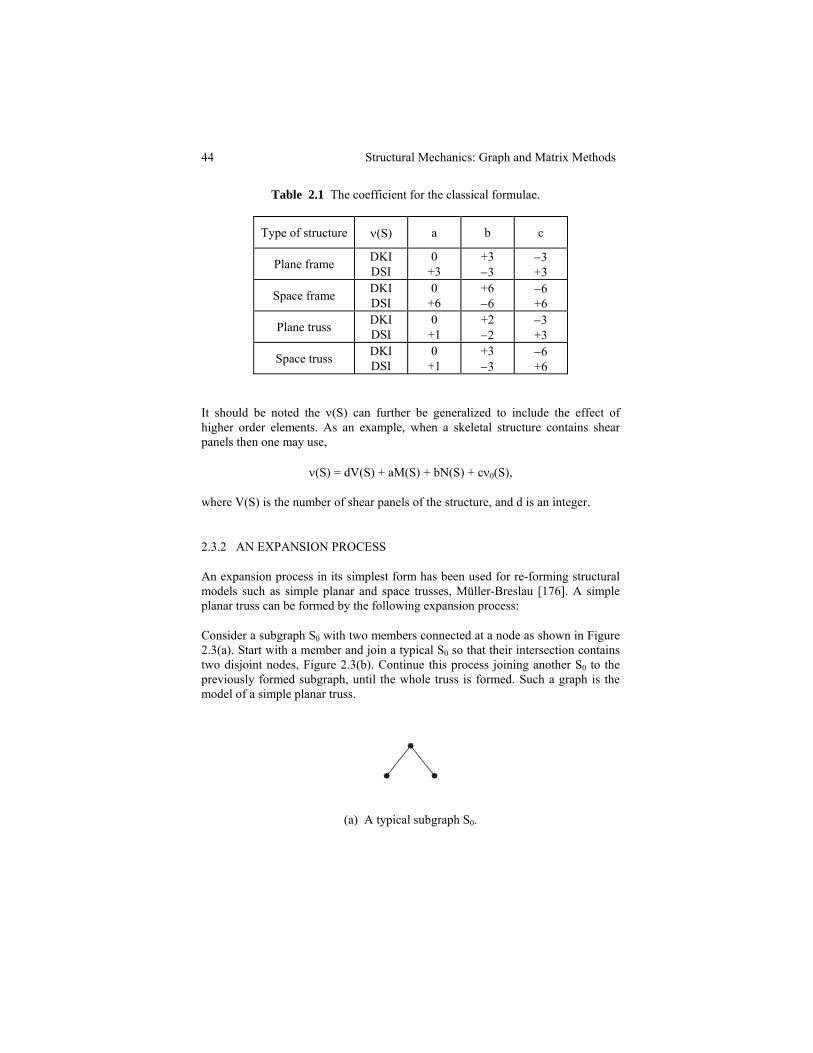
Consider a subgraph S0 with two members connected at a node as shown in Figure 2.3(a). Start with a member and join a typical S0 so that their intersection contains two disjoint nodes, Figure 2.3(b). Continue this process joining another S0 to the previously formed subgraph, until the whole truss is formed. Such a graph is the model of a simple planar truss.
(a) A typical subgraph S0.
CHAPTER 2 Topological Properties of Skeletal Structures 45
S1=S1 → S2=S1 ∪ S0 → S3=S2 ∪ S0 → S4=S3 ∪ S0 → S5=S4 ∪ S0
(b) An expansion process.
Fig. 2.3 Formation of a planar simple truss.
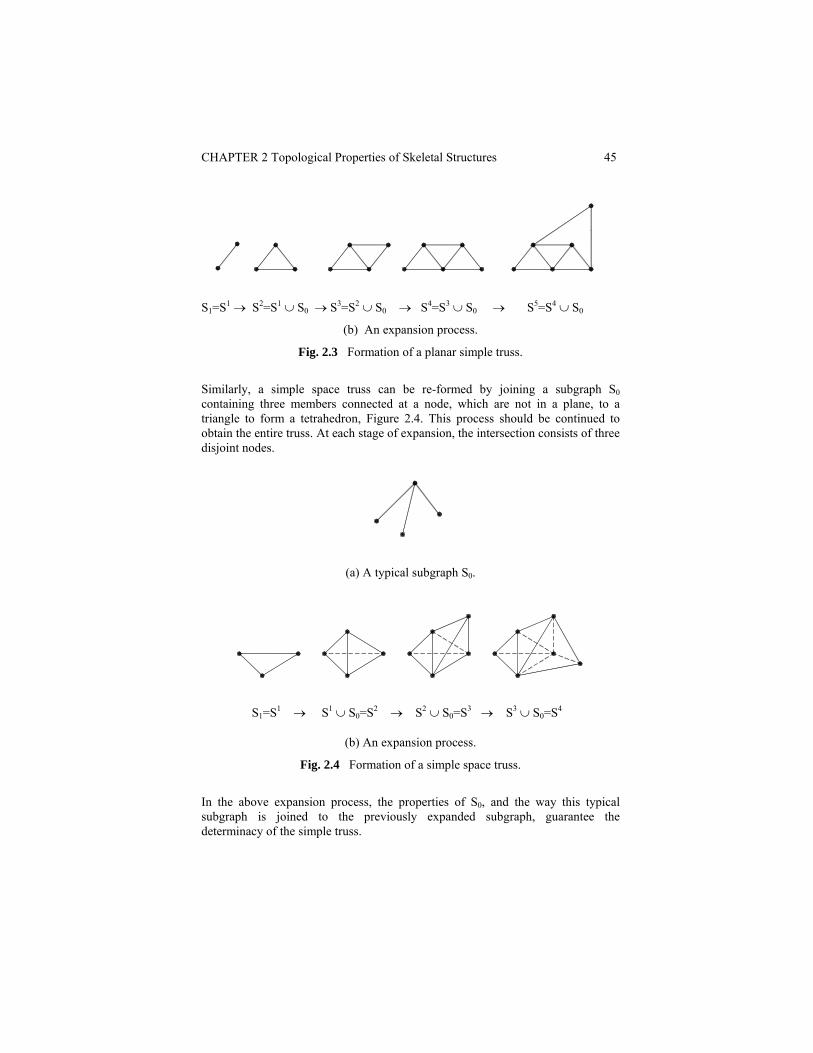
Similarly, a simple space truss can be re-formed by joining a subgraph S0 containing three members connected at a node, which are not in a plane, to a triangle to form a tetrahedron, Figure 2.4. This process should be continued to obtain the entire truss. At each stage of expansion, the intersection consists of three disjoint nodes.
(a) A typical subgraph S0.
S1=S1 → S1 ∪ S0=S2 → S2 ∪ S0=S3 → S3 ∪ S0=S4
(b) An expansion process.
Fig. 2.4 Formation of a simple space truss.
In the above expansion process, the properties of S0, and the way this typical subgraph is joined to the previously expanded subgraph, guarantee the determinacy of the simple truss.
46 Structural Mechanics: Graph and Matrix Methods
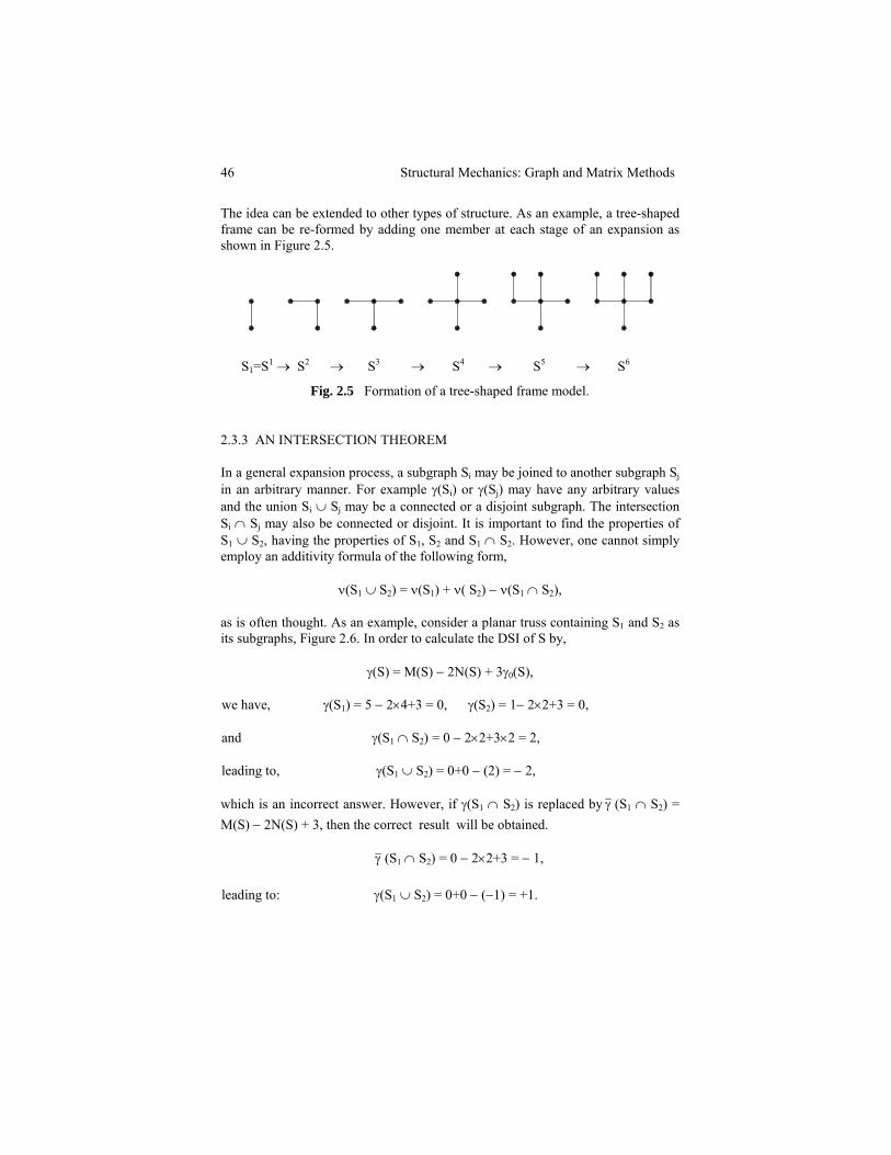
The idea can be extended to other types of structure. As an example, a tree-shaped frame can be re-formed by adding one member at each stage of an expansion as shown in Figure 2.5.
S1=S1 → S2 → S3 → S4 → S5 → S6
Fig. 2.5 Formation of a tree-shaped frame model.
2.3.3 AN INTERSECTION THEOREM
In a general expansion process, a subgraph Si may be joined to another subgraph Sj in an arbitrary manner. For example γ(Si) or γ(Sj) may have any arbitrary values and the union Si ∪ Sj may be a connected or a disjoint subgraph. The intersection Si ∩ Sj may also be connected or disjoint. It is important to find the properties of S1 ∪ S2, having the properties of S1, S2 and S1 ∩ S2. However, one cannot simply employ an additivity formula of the following form,
ν(S1 ∪ S2) = ν(S1) + ν( S2) − ν(S1 ∩ S2),
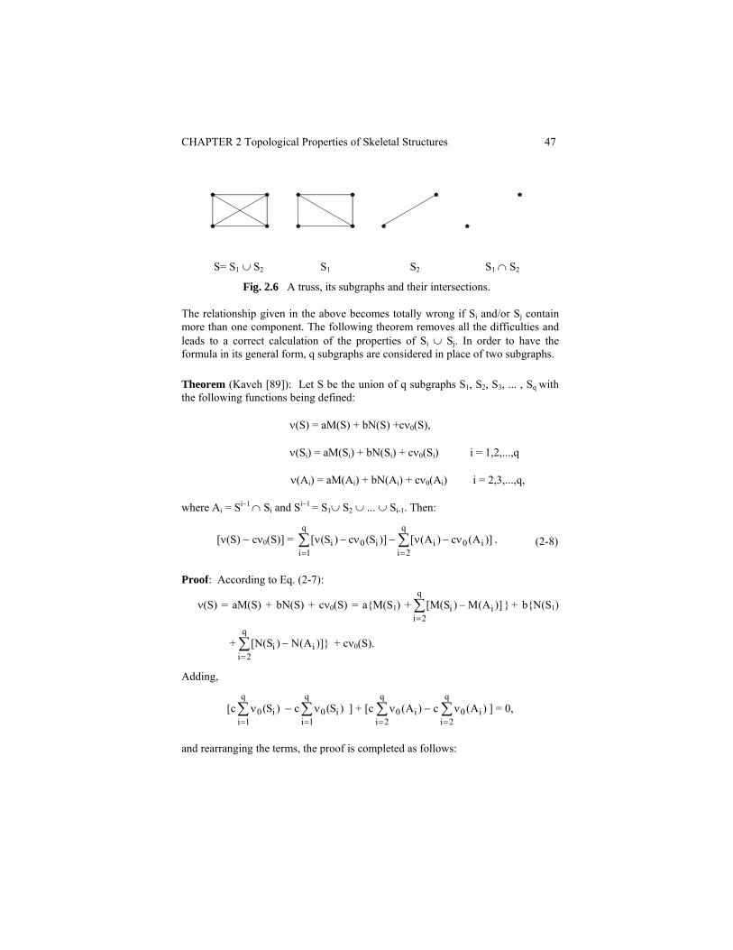
as is often thought. As an example, consider a planar truss containing S1 and S2 as its subgraphs, Figure 2.6. In order to calculate the DSI of S by,
γ(S) = M(S) − 2N(S) + 3γ0(S),
we have, γ(S1) = 5 − 2×4+3 = 0, γ(S2) = 1− 2×2+3 = 0,
and γ(S1 ∩ S2) = 0 − 2×2+3×2 = 2,
leading to, γ(S1 ∪ S2) = 0+0 − (2) = − 2,
which is an incorrect answer. However, if γ(S1 ∩ S2) is replaced by γ (S1 ∩ S2) = M(S) − 2N(S) + 3, then the correct result will be obtained.
γ (S1 ∩ S2) = 0 − 2×2+3 = − 1,
leading to: γ(S1 ∪ S2) = 0+0 − (−1) = +1.
CHAPTER 2 Topological Properties of Skeletal Structures 47
S= S1 ∪ S2 S1 S2 S1 ∩ S2
Fig. 2.6 A truss, its subgraphs and their intersections.
The relationship given in the above becomes totally wrong if Si and/or Sj contain more than one component. The following theorem removes all the difficulties and leads to a correct calculation of the properties of Si ∪ Sj. In order to have the formula in its general form, q subgraphs are considered in place of two subgraphs.
Theorem (Kaveh [89]): Let S be the union of q subgraphs S1, S2, S3, ... , Sq with the following functions being defined:
ν(S) = aM(S) + bN(S) +cν0(S),
ν(Si) = aM(Si) + bN(Si) + cν0(Si) i = 1,2,...,q
ν(Ai) = aM(Ai) + bN(Ai) + cν0(Ai) i = 2,3,...,q,
where Ai = Si−1 ∩ Si and Si−1 = S1∪ S2 ∪ ... ∪ Si-1. Then:
[ν(S) − cν0(S)] = ∑
=ν−ν
q
1ii0i )]S(c)S([ − ∑
=ν−ν
q
2ii0i )]A(c)A([ . (2-8)
Proof: According to Eq. (2-7):
ν(S) = aM(S) + bN(S) + cν0(S) = a{M(S1) + } ])A(M )[M(Sq
2iii∑
=− + b{N(S1)
+ ∑=
−q
2iii ]})A(N )[N(S + cν0(S).
Adding,
[c ∑=
νq
1ii0 )S( − c ∑
= ν
q
1ii0 )S( ] + [c ∑
=ν
q
2ii0 )A( − c ∑
=ν
q
2ii0 )A( ] = 0,
and rearranging the terms, the proof is completed as follows:
48 Structural Mechanics: Graph and Matrix Methods
[ν(S) − cν0(S)] = ∑=
ν++q
1ii0ii )]S(c)S(bN)S(aM[
− ∑=
ν++q
2ii0ii )]A(c)A(bN)A(aM[ − c ∑
= ν
q
1ii0 )S( + c ∑
=ν
q
2ii0 )A(
= ])S(cv)S([q
1ii0i∑
=−ν − ∑
=ν−ν
q
2ii0i )]A(c)A([ .
Special Case: If S and each of its subgraphs considered for expansion (Si for i = 1,...,q) are non-disjoint (connected), then Eq. (2-8) can be simplified as,
ν(S) = ∑=
νq
1ii )S( − ∑
=ν
q
2ii )(A , (2-9)
where: ν (Ai) = aM(Ai) +bN(Ai) + c.
For calculating the DKI and DSI of a complex structure or a structure with a large number of members, one normally selects a repeated unit of the structure and joins these units sequentially in a connected form. Thus, Eq. (2-9) can be applied in place of Eq. (2-8) to obtain the overall property of the structure.
2.3.4 A METHOD FOR DETERMINING THE DKI AND DSI OF STRUCTURES
Let S be the union of its repeated and/or simple pattern subgraphs Si (i=1,...,q). Calculate the DKI or DSI of each subgraph using the appropriate coefficients from Table 2.1. Now perform the following steps:
Step 1. Join S1 to S2 to form S2 = S1 ∪ S2, and calculate the DKI or DSI of their intersection A2 = S1 ∩ S2. The value of ν(S2) can be found using Eq. (2-8) or Eq. (2-9), as appropriate.
Step 2. Join S3 to S2 to obtain S3 = S2 ∪ S3, and determine the DKI or DSI of A3 = S2 ∩ S3. Similarly to Step 1, calculate ν(S3).
Step k. Subsequently join Sk+1 to Sk, calculating the DKI or DSI of Ak+1 = Sk ∩
Sk+1 and evaluating the magnitude of ν(Sk+1).
CHAPTER 2 Topological Properties of Skeletal Structures 49
Repeat Step k until the entire structural model iq
1iSS
=∪= is reformed and its DKI or
DSI is determined.
In the above expansion process, the value of q depends on the properties of the substructures (subgraphs) which are considered for reforming S. These subgraphs have either simple patterns for which ν(Si) can easily be calculated, or the value of their DKI or DSI are already known.
In the process of expansion, if an intersection Ai itself has a complex pattern, further refinement is also possible; i.e. the intersection can be considered as the union of simpler subgraphs.
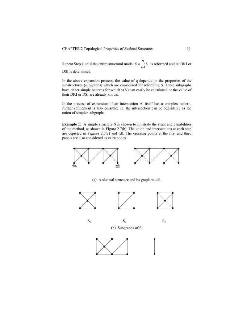
Example 1: A simple structure S is chosen to illustrate the steps and capabilities of the method, as shown in Figure 2.7(b). The union and intersections at each step are depicted in Figures 2.7(c) and (d). The crossing points at the first and third panels are also considered as extra nodes.
(a) A skeletal structure and its graph model.
S1 S2 S3
(b) Subgraphs of S.
50 Structural Mechanics: Graph and Matrix Methods
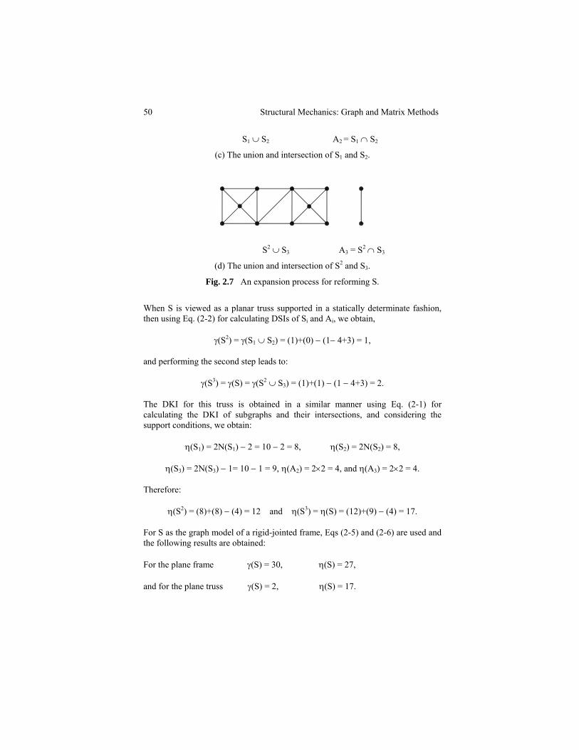
S1 ∪ S2 A2 = S1 ∩ S2
(c) The union and intersection of S1 and S2.
S2 ∪ S3 A3 = S2
∩ S3
(d) The union and intersection of S2 and S3.
Fig. 2.7 An expansion process for reforming S.
When S is viewed as a planar truss supported in a statically determinate fashion, then using Eq. (2-2) for calculating DSIs of Si and Ai, we obtain,
γ(S2) = γ(S1 ∪ S2) = (1)+(0) − (1− 4+3) = 1,
and performing the second step leads to:
γ(S3) = γ(S) = γ(S2 ∪ S3) = (1)+(1) − (1 − 4+3) = 2.
The DKI for this truss is obtained in a similar manner using Eq. (2-1) for calculating the DKI of subgraphs and their intersections, and considering the support conditions, we obtain:
η(S1) = 2N(S1) − 2 = 10 − 2 = 8, η(S2) = 2N(S2) = 8,
η(S3) = 2N(S3) − 1= 10 − 1 = 9, η(A2) = 2×2 = 4, and η(A3) = 2×2 = 4.
Therefore:
η(S2) = (8)+(8) − (4) = 12 and η(S3) = η(S) = (12)+(9) − (4) = 17.
For S as the graph model of a rigid-jointed frame, Eqs (2-5) and (2-6) are used and the following results are obtained:
For the plane frame γ(S) = 30, η(S) = 27,
and for the plane truss γ(S) = 2, η(S) = 17.
CHAPTER 2 Topological Properties of Skeletal Structures 51
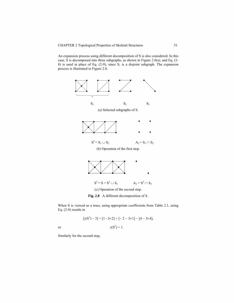
An expansion process using different decomposition of S is also considered. In this case, S is decomposed into three subgraphs, as shown in Figure 2.8(a), and Eq. (2-8) is used in place of Eq. (2-9), since S1 is a disjoint subgraph. The expansion process is illustrated in Figure 2.8.
S1 S2 S3
(a) Selected subgraphs of S.
S2 = S1 ∪ S2 A2 = S1 ∩ S2
(b) Operation of the first step.
S3 = S = S2 ∪ S3 A3 = S2
∩ S3 (c) Operation of the second step.
Fig. 2.8 A different decomposition of S.
When S is viewed as a truss, using appropriate coefficients from Table 2.1, using Eq. (2-8) results in
[γ(S2) − 3] = [1 −3×2] + [− 2 − 3×1] − [4 − 3×4],
or γ(S2) = 1.
Similarly for the second step,
52 Structural Mechanics: Graph and Matrix Methods
[γ(S3) − 3] = [1 − 3×1] + [0 − 3×1] − [− 4+6 − 3×2],
or γ(S3) = γ(S) = 2.
In order to calculate the DKI, Eq. (2-7) is used for determining the DKIs of the subgraphs and intersections (with appropriate coefficients from Table 2.1), and the same results as the previous ones are obtained.
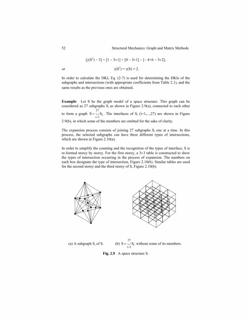
Example: Let S be the graph model of a space structure. This graph can be considered as 27 subgraphs Si as shown in Figure 2.9(a), connected to each other
to form a graph i27
1iSS
=∪= . The interfaces of Si (i=1,...,27) are shown in Figure
2.9(b), in which some of the members are omitted for the sake of clarity.
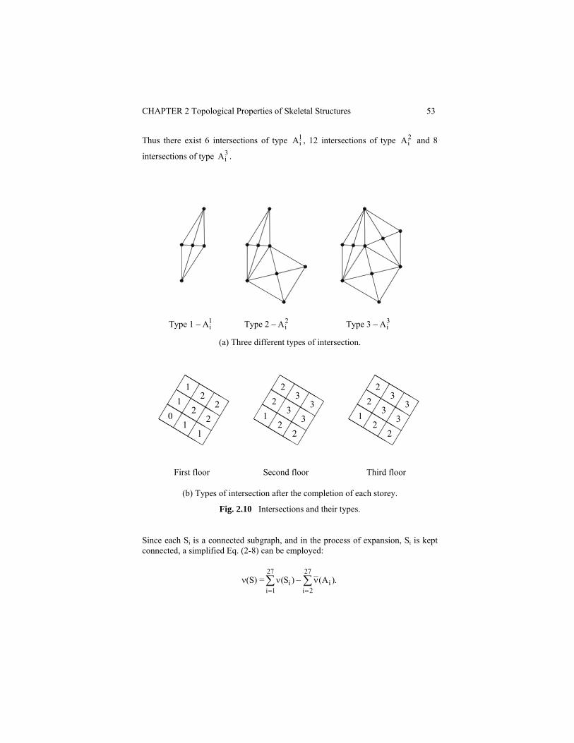
The expansion process consists of joining 27 subgraphs Si one at a time. In this process, the selected subgraphs can have three different types of intersections, which are shown in Figure 2.10(a).
In order to simplify the counting and the recognition of the types of interface, S is re-formed storey by storey. For the first storey, a 3×3 table is constructed to show the types of intersection occurring in the process of expansion. The numbers on each box designate the type of intersection, Figure 2.10(b). Similar tables are used for the second storey and the third storey of S, Figure 2.10(b).
(a) A subgraph Si of S. (b) i27
1iSS
=∪= without some of its members.
Fig. 2.9 A space structure S.
CHAPTER 2 Topological Properties of Skeletal Structures 53
Thus there exist 6 intersections of type 1
iA , 12 intersections of type 2iA and 8
intersections of type 3iA .
Type 1 − 1iA Type 2 − 2
iA Type 3 − 3iA
(a) Three different types of intersection.
01
12
21
12
21
22
33
22
33
22
1 33
22
33
First floor Second floor Third floor
(b) Types of intersection after the completion of each storey.
Fig. 2.10 Intersections and their types.
Since each Si is a connected subgraph, and in the process of expansion, Si is kept connected, a simplified Eq. (2-8) can be employed:
ν(S) = ∑=
ν27
1ii )S( − .)A(
27
2ii∑
=ν
54 Structural Mechanics: Graph and Matrix Methods
As has been shown:
∑=
ν27
2ii )A( = .)A()A()A(
27
20i
3i
19
8i
2i
7
2i
1i ∑∑∑
===ν+ν+ν
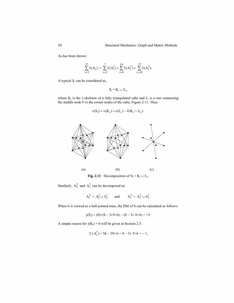
A typical Si can be considered as,
Si = Ki ∪ Li,
where Ki is the 1-skeleton of a fully triangulated cube and Li is a star connecting the middle node F to the corner nodes of the cube, Figure 2.11. Thus:
)LK()L()K()S( iiiii ∩ν−ν+ν=ν .
(a) (b) (c)
Fig. 2.11 Decomposition of Si = Ki ∪ Li.
Similarly, 2iA and 3
iA can be decomposed as:
2iA = 1
iA ∪ 1iA and 3
iA = 2iA ∪ 1
iA .
When S is viewed as a ball-jointed truss, the DSI of S can be calculated as follows:
γ(Si) = (0)+(8 − 3×9+6) − (0 − 3× 8+6) = +5.
A simple reason for γ(Ki) = 0 will be given in Section 2.5.
γ ( 1iA ) = M − 3N+6 = 8 − 3× 5+6 = − 1,
CHAPTER 2 Topological Properties of Skeletal Structures 55
γ ( 2
iA ) = (−1)+( −1) − (1−3×2+6) = − 3,
γ ( 3iA ) = (−1)+( −3) − (2−3×3+6) = − 3.
Hence: γ(S) = 27(5) − [6(−1)+12(−3)+8(−3)] = 201.
When S is taken as a space rigid-jointed frame, then γ(S) = 3564 is obtained.
Similar calculations are performed for determining the DKI of S, and η(S) = 591 and η(S) = 1188 are obtained for ball-jointed truss and space frame, respectively.
The union-intersection method becomes very efficient for structures with repeated patterns. Counting is reduced considerably by this method. As an example, the use of the classical formula for finding the DSI of S in the above example requires counting 792 members and 199 nodes, which is not an easy task with a probable mistake in the process of counting.
2.3.5 MODIFICATIONS ON A STRUCTURE
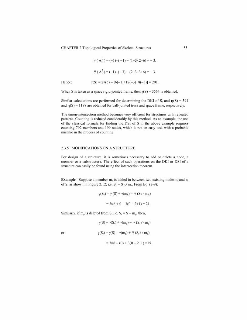
For design of a structure, it is sometimes necessary to add or delete a node, a member or a substructure. The effect of such operations on the DKI or DSI of a structure can easily be found using the intersection theorem.
Example: Suppose a member mk is added in between two existing nodes ni and nj of S, as shown in Figure 2.12; i.e. Sc = S ∪ mk. From Eq. (2-9):
γ(Sc) = γ (S) + γ(mk) − γ (S ∩ mk)
= 3×6 + 0 − 3(0 − 2+1) = 21.
Similarly, if mp is deleted from S, i.e. Sr = S − mp, then,
γ(S) = γ(Sr) + γ(mp) − γ (Sr ∩ mp)
or γ(Sr) = γ(S) − γ(mp) + γ (Sr ∩ mp)
= 3×6 − (0) + 3(0 − 2+1) =15.
56 Structural Mechanics: Graph and Matrix Methods
m p
n i
jn
m k
(a) S (b) Sc (c) Sr
Fig. 2.12 Modifications on a planar frame.
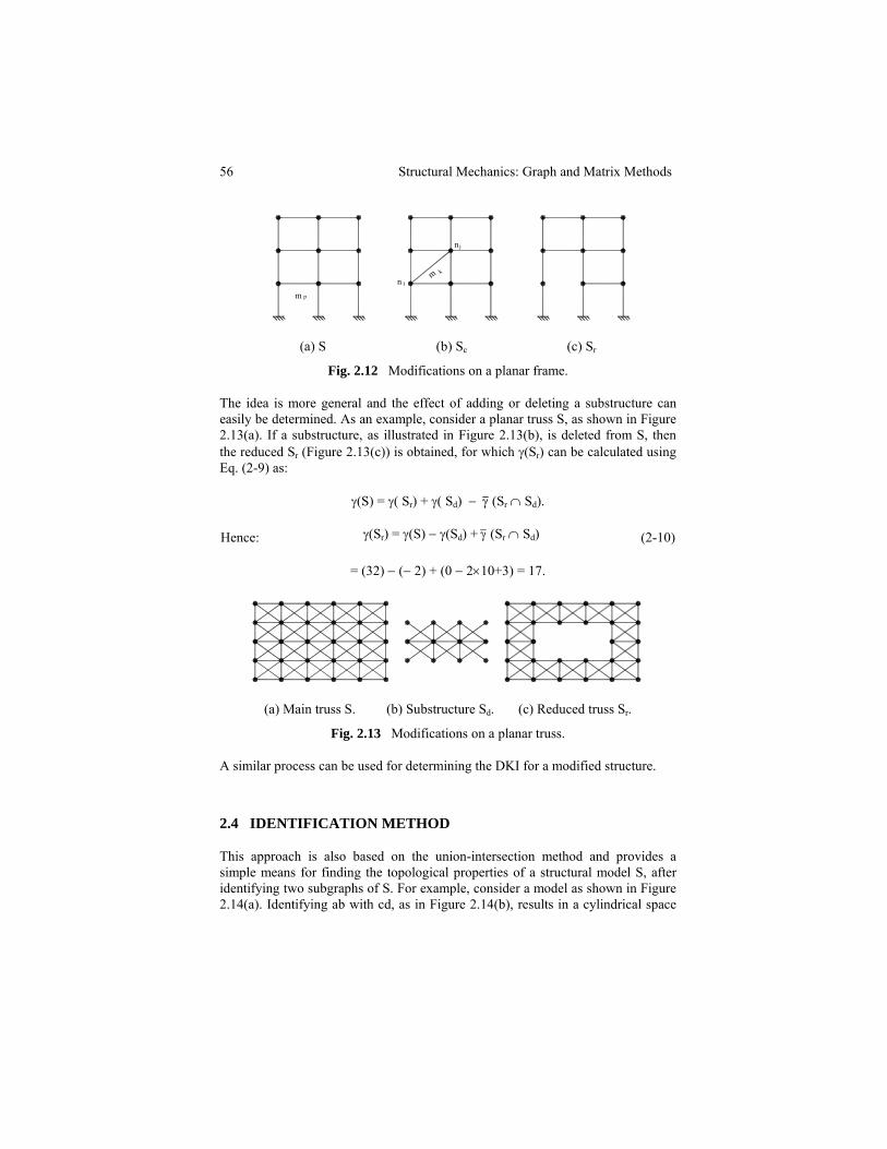
The idea is more general and the effect of adding or deleting a substructure can easily be determined. As an example, consider a planar truss S, as shown in Figure 2.13(a). If a substructure, as illustrated in Figure 2.13(b), is deleted from S, then the reduced Sr (Figure 2.13(c)) is obtained, for which γ(Sr) can be calculated using Eq. (2-9) as:
γ(S) = γ( Sr) + γ( Sd) − γ (Sr ∩ Sd).
Hence: γ(Sr) = γ(S) − γ(Sd) + γ (Sr ∩ Sd) (2-10)
= (32) − (− 2) + (0 − 2×10+3) = 17.
(a) Main truss S. (b) Substructure Sd. (c) Reduced truss Sr.
Fig. 2.13 Modifications on a planar truss.
A similar process can be used for determining the DKI for a modified structure.
2.4 IDENTIFICATION METHOD
This approach is also based on the union-intersection method and provides a simple means for finding the topological properties of a structural model S, after identifying two subgraphs of S. For example, consider a model as shown in Figure 2.14(a). Identifying ab with cd, as in Figure 2.14(b), results in a cylindrical space
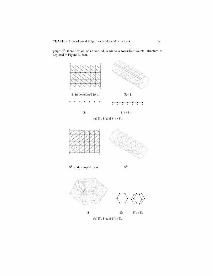
CHAPTER 2 Topological Properties of Skeletal Structures 57
graph S2. Identification of ac and bd, leads to a torus-like skeletal structure as depicted in Figure 2.14(c).
a b
c d S1 in developed form S1= S1
S2 S1 ∩ S2
(a) S1, S2 and S1 ∩ S2.
a b
a b
S2 in developed form S2
S2 S3 S2 ∩ S3
(b) S2, S3 and S2 ∩ S3.
58 Structural Mechanics: Graph and Matrix Methods
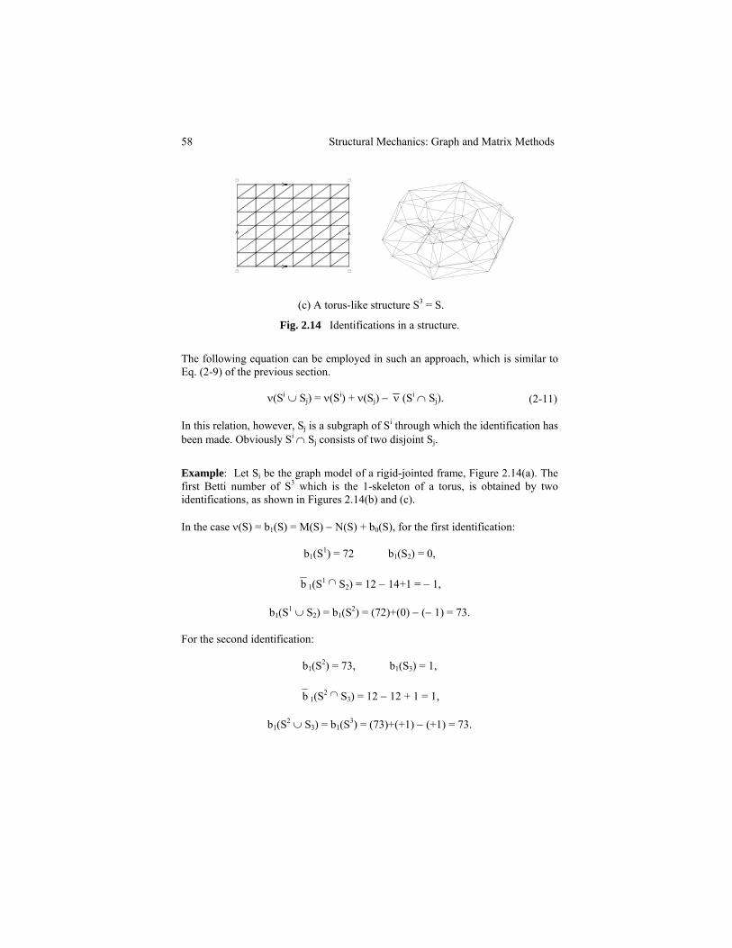
(c) A torus-like structure S3 = S.
Fig. 2.14 Identifications in a structure.
The following equation can be employed in such an approach, which is similar to Eq. (2-9) of the previous section.
ν(Si ∪ Sj) = ν(Si) + ν(Sj) − ν (Si ∩ Sj). (2-11)
In this relation, however, Sj is a subgraph of Si through which the identification has been made. Obviously Si ∩ Sj consists of two disjoint Sj.
Example: Let Si be the graph model of a rigid-jointed frame, Figure 2.14(a). The first Betti number of S3 which is the 1-skeleton of a torus, is obtained by two identifications, as shown in Figures 2.14(b) and (c).
In the case ν(S) = b1(S) = M(S) − N(S) + b0(S), for the first identification:
b1(S1) = 72 b1(S2) = 0,
b 1(S1 ∩ S2) = 12 − 14+1 = − 1,
b1(S1 ∪ S2) = b1(S2) = (72)+(0) − (− 1) = 73.
For the second identification:
b1(S2) = 73, b1(S3) = 1,
b 1(S2 ∩ S3) = 12 − 12 + 1 = 1,
b1(S2 ∪ S3) = b1(S3) = (73)+(+1) − (+1) = 73.
CHAPTER 2 Topological Properties of Skeletal Structures 59
When S is viewed as a space frame, the DSI can easily be found as γ(S) = 6b1(S) = 6×73 = 438. For S viewed as a ball-jointed truss, the DSI can be determined as follows:
For the first identification:
γ(S1) = M − 3N+6 = 120 − 3×49+6 = − 21,
γ(S2) = 6 − 3×7+6 = − 9,
γ (S1 ∩ S2) = 12 − 3×14+6 = −24,
γ(S1 ∪ S2) = γ(S2) = (− 21)+( − 9) − (− 24) = − 6.
For the second identification:
γ(S2) = − 6, γ(S3) = 6 − 3×6+6 = − 6,
γ (S2 ∩ S3) = 12 − 3×12+6 = − 18,
γ(S2 ∪ S3) = γ(S3) = (− 6)+( − 6) − (− 18) = 6.
2.5 THE DSI OF STRUCTURES: SPECIAL METHODS
In this section, using Euler´s polyhedra formula (Section 1.8.1), some useful theorems are proven, which provide simple means for calculating the DSI of various types of skeletal structures.
Theorem 1: For a fully triangulated planar truss (except the exterior boundary), the internal DSI is the same as the number of its internal nodes:
γ(S) = Ni(S). (2-12)
Proof: Draw S in the plane. According to Euler´s formula,
R(S) − M(S) + N(S) = 2, (2-13)
where R(S) = Ri(S) + 1 is the total number of regions and Ri(S) is the number of triangles. Since all the internal regions are triangles,
3Ri(S) = 2M(S) − Me(S), (2-14)
60 Structural Mechanics: Graph and Matrix Methods
Me(S) being the number of members in the exterior boundary of S which may be any polygon. Substituting,
Me(S) = Ne(S) = N(S) − Ni(S), (2-15)
in Eq. (2-14) leads to:
3Ri(S) = 2M(S) − Ne(S) = 2M(S) − N(S) + Ni(S). (2-16)
From Eq. (2-13), we have:
Ri(S) = M(S) − N(S) + 1. (2-17)
Substituting from Eq. (2-17) in Eq. (2-16) yields:
M(S) − 2N(S) + 3 = Ni(S).
Thus: γ(S) = Ni(S).
For trusses with non-triangulated internal regions (Figure 2.15(a)), let Mci(S) be the number of members required for completion of the triangulation of the internal regions of S, then:
γ(S) = Ni(S) − Mci(S). (2-18)
The number of members required for triangulation of a polygon is constant and independent of the way it is triangulated. This is why Eq. (2-18) can easily be established.
Once the internal DSI of a structure is found, the external DSI resulting from the additional supports can easily be added, to obtain the total DSI.
Example: For the truss shown in Figure 2.13(a), the application of Eq. (2-12) results in:
γ(S) = Ni(S) = 32.
The use of the classical formula (Eq. (2-2)) leads to the same result,
γ(S) = 129 − 2×50 + 3 = 32,
but it necessitates counting 129 members and 50 nodes, compared with counting 32 internal nodes.
CHAPTER 2 Topological Properties of Skeletal Structures 61
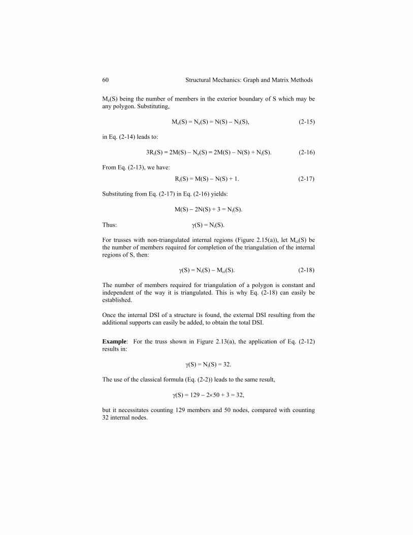
Example: Let S be a planar truss as shown in Figure 2.15. Triangulation of the internal region in an arbitrary manner requires 9 members, shown as dashed lines. Thus γ(S) = Ni(S) − Mci(S) = 16 − 9 = 7.
(a) A planar truss S. (b) Triangulated S.
Fig. 2.15 A general planar truss and its triangulation.
Theorem 2: The DSI of a planar rigid-jointed frame S is equal to three times the number of its internal regions,
γ(S) = 3Ri(S). (2-19)
Proof: A tree structure is statically determinate. For each addition of a chord the indeterminacy of the structure increases by 3, and therefore:
γ(S) = 3[M(S) − N(S) + 1].
Using Eq. (2-17) completes the proof, i.e.
γ(S) = 3Ri(S).
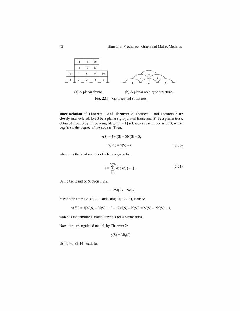
Example: The DSI of the rigid-jointed plane frame shown in Figure 2.16(a) is obtained as,
γ(S) = 3Ri(S) = 3×16 = 48,
and for the rigid-jointed arch-type structure of Figure 2.16(b), we have:
γ(S) = 3×6 = 18.
Obviously, the classical formula (Eq. (2-6)) requires more counting than the above method.
62 Structural Mechanics: Graph and Matrix Methods
1 2 3 4 5
109876
11 12 13
161514
64 5
1 2 3
(a) A planar frame. (b) A planar arch-type structure.
Fig. 2.16 Rigid-jointed structures.
Inter-Relation of Theorem 1 and Theorem 2: Theorem 1 and Theorem 2 are closely inter-related. Let S be a planar rigid-jointed frame and S′ be a planar truss, obtained from S by introducing [deg (ni) − 1] releases in each node ni of S, where deg (ni) is the degree of the node ni. Then,
γ(S) = 3M(S) − 3N(S) + 3,
γ( S′ ) = γ(S) − r, (2-20)
where r is the total number of releases given by:
r = ∑=
−N(S)
1ii 1])(n [deg . (2-21)
Using the result of Section 1.2.2,
r = 2M(S) − N(S).
Substituting r in Eq. (2-20), and using Eq. (2-19), leads to,
γ( S′ ) = 3[M(S) − N(S) + 1] − [2M(S) − N(S)] = M(S) − 2N(S) + 3,
which is the familiar classical formula for a planar truss.
Now, for a triangulated model, by Theorem 2:
γ(S) = 3Ri(S).
Using Eq. (2-14) leads to:
CHAPTER 2 Topological Properties of Skeletal Structures 63
γ(S) = 2M(S) − Me(S).
On the other hand,
γ( S′ ) = γ(S) − [2M(S) − N(S)] = [2M(S) − Me(S)] − [2M(S) − N(S)]
= N(S) − Me(S) = N(S) − Ne(S) = Ni(S),
which is the same result as that of Theorem 1.
Using a reverse process, by introducing constraints in place of releases, a truss model S′ can be changed to a frame model S, and Eq. (2-19) can be derived from Eq. (2-12).
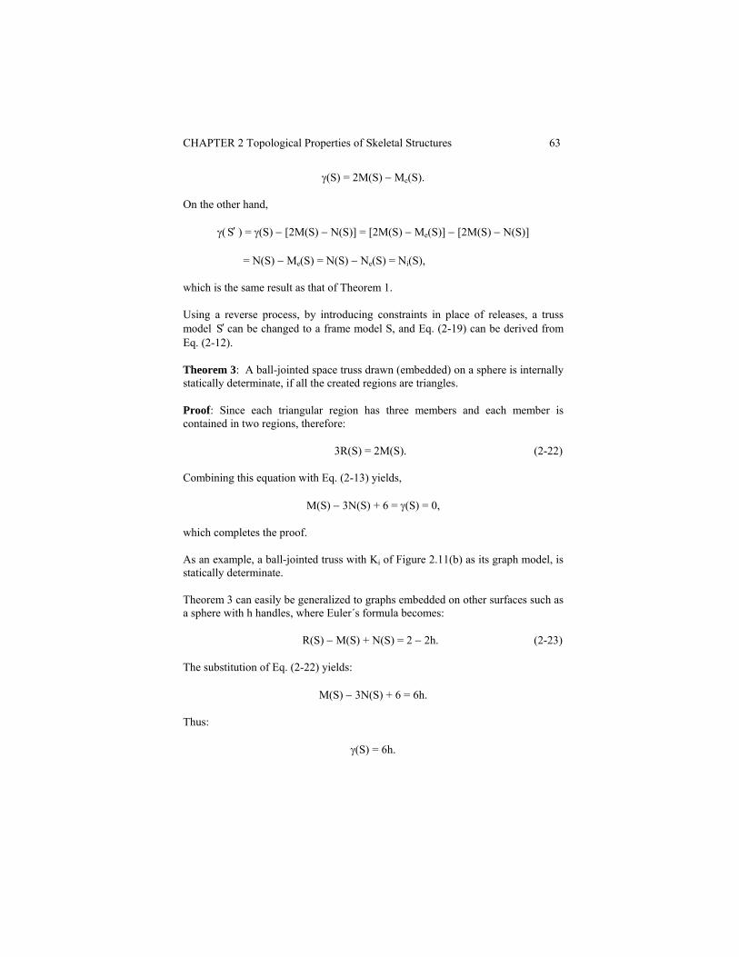
Theorem 3: A ball-jointed space truss drawn (embedded) on a sphere is internally statically determinate, if all the created regions are triangles.
Proof: Since each triangular region has three members and each member is contained in two regions, therefore:
3R(S) = 2M(S). (2-22)
Combining this equation with Eq. (2-13) yields,
M(S) − 3N(S) + 6 = γ(S) = 0,
which completes the proof.
As an example, a ball-jointed truss with Ki of Figure 2.11(b) as its graph model, is statically determinate.
Theorem 3 can easily be generalized to graphs embedded on other surfaces such as a sphere with h handles, where Euler´s formula becomes:
R(S) − M(S) + N(S) = 2 − 2h. (2-23)
The substitution of Eq. (2-22) yields:
M(S) − 3N(S) + 6 = 6h.
Thus:
γ(S) = 6h.
64 Structural Mechanics: Graph and Matrix Methods
As an example, the DSI of a triangulated space truss in the form of a torus (sphere with one handle), shown in Figure 2.17, becomes γ(S) = 6×1 = 6.
Fig. 2.17 The 1-skeleton of a triangulated torus.
2.6 SPACE STRUCTURES AND THEIR PLANAR DRAWINGS
In this section methods are developed for transforming the topological properties of space structures into those of their planar drawings, thus simplifying the counting process for the calculation of the DSI for space structures.
2.6.1 ADMISSIBLE DRAWING OF A SPACE STRUCTURE
A drawing Sp of a graph S in the plane is a mapping of the nodes of S to distinct points of Sp, and the members of S to open arcs of Sp such that:
(i) the image of no member contains that of any node;
(ii) the image of a member (ni,nj) joins the points corresponding to ni and nj.
A drawing is called admissible (good) if the members are such that:
(iii) no two arcs with a common end point meet;
(iv) no two arcs meet in more than one point;
(v) no three arcs meet in a common point.
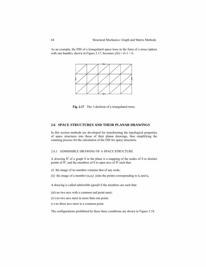
The configurations prohibited by these three conditions are shown in Figure 2.18.
CHAPTER 2 Topological Properties of Skeletal Structures 65
Fig. 2.18 The prohibited configurations.
A point of intersection of two members in a drawing is called a crossing, and the crossing number c(Sp) of a graph S is the number of crossings in any admissible drawing of S in the plane. An optimal drawing in a given surface is one which exhibits the least possible crossings. In this book we will use only admissible drawings in the plane, but not necessarily optimal.
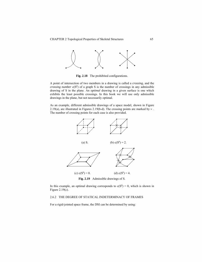
As an example, different admissible drawings of a space model, shown in Figure 2.19(a), are illustrated in Figures 2.19(b-d). The crossing points are marked by × . The number of crossing points for each case is also provided.
(a) S. (b) c(Sp) = 2.
(c) c(Sp) = 0. (d) c(Sp) = 4.
Fig. 2.19 Admissible drawings of S.
In this example, an optimal drawing corresponds to c(Sp) = 0, which is shown in Figure 2.19(c).
2.6.2 THE DEGREE OF STATICAL INDETERMINACY OF FRAMES
For a rigid-jointed space frame, the DSI can be determined by using:
66 Structural Mechanics: Graph and Matrix Methods
γ(S) = 6[M(S) − N(S) +1]. (2-24)
Counting the nodes in a drawing of S on the plane produces no problem, however, recognition and counting the members can be very cumbersome. The following theorem transforms this procedure to counting the crossing nodes and regions of Sp, in place of members and nodes of S.
Theorem: For a space rigid-jointed frame, the DSI is given by:
γ(S) = 6[Ri(Sp) − c(Sp)]. (2-25)
Proof: Once a space structure is drawn in the plane, the following relationships can be established between the numbers of members and nodes of S and Sp:
M(Sp) = M(S) + 2c(Sp) and N(Sp) = N(S) + c(Sp). (2-26)
Substituting the above equations in Eq. (2-24) yields:
γ(S) = 6[M(Sp) − 2c(Sp) − N(Sp) + c(Sp) + 1]
= 6[M(Sp) − N(Sp) + 1 − c(Sp)].
However, for a planar drawing:
M(Sp) − N(Sp) + 1 = Ri(Sp).
Hence:
γ(S) = 6[Ri(Sp) − c(Sp)].
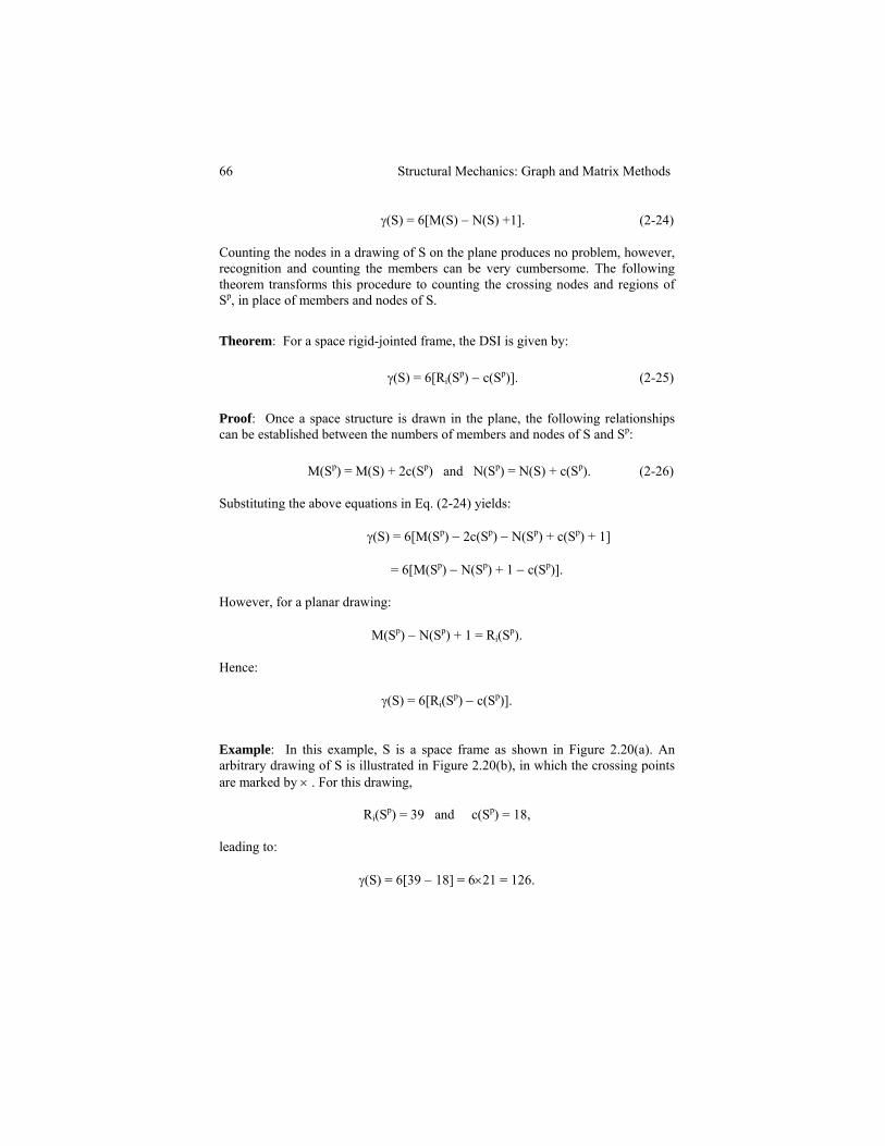
Example: In this example, S is a space frame as shown in Figure 2.20(a). An arbitrary drawing of S is illustrated in Figure 2.20(b), in which the crossing points are marked by × . For this drawing,
Ri(Sp) = 39 and c(Sp) = 18,
leading to:
γ(S) = 6[39 − 18] = 6×21 = 126.
CHAPTER 2 Topological Properties of Skeletal Structures 67
1 2 3
39
(a) A space frame S. (b) An arbitrary drawing of S.
21
20
19
18
1
2
3
4
5
6
7
8
9
10
1213
1411
15
1617
(c) An optimal drawing of S.
Fig. 2.20 A space frame and its drawings.
From Eq. (2-24) one can also calculate the DSI as,
γ(S) = 6[44 − 24+1] = 126,
which requires 44+24=68 countings in comparison to 39+18=57 countings in the present method. This number can further be improved by constructing a drawing with a smaller number of crossings. The ideal situation corresponds to an optimal drawing. For this example, an optimal drawing is shown in Figure 2.20(c), for which,
Ri(Sp) = 21 and c(Sp) = 0,
leading to: γ(S) = 6(21− 0) = 126.
In this case the number of countings is reduced to 21.
68 Structural Mechanics: Graph and Matrix Methods
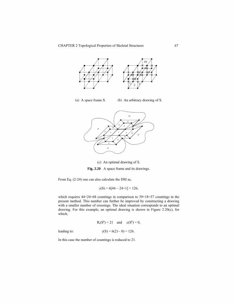
Example: Let S be the graph model of a space frame as shown in Figure 2.21(a). A drawing Sp of S is shown in Figure 2.21(b) for which c(Sp) = 8 and Ri(Sp) = 41, resulting in γ(S) = 6[41 − 8] = 198.
(a) A space frame S. (b) A drawing of S.
Fig. 2.21 A space frame and its drawing.
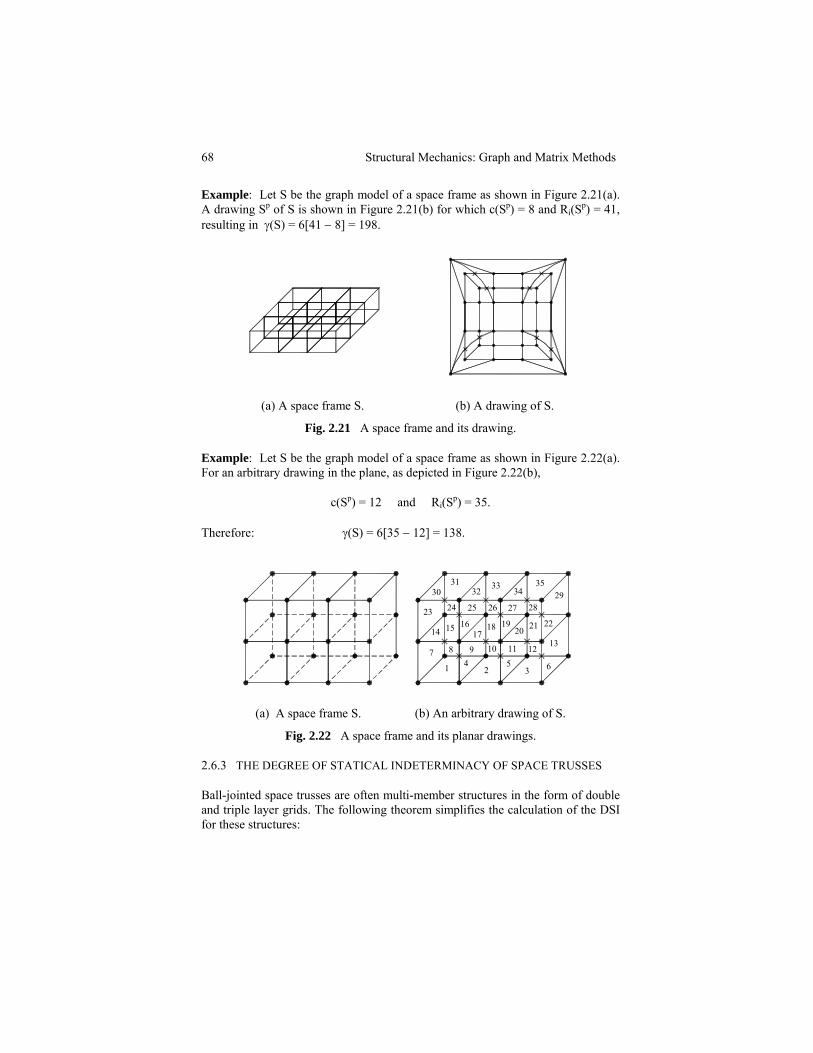
Example: Let S be the graph model of a space frame as shown in Figure 2.22(a). For an arbitrary drawing in the plane, as depicted in Figure 2.22(b),
c(Sp) = 12 and Ri(Sp) = 35.
Therefore: γ(S) = 6[35 − 12] = 138.
3031 33 35
2932 34
282726252423
14 15 1617
18 1920 21 22
13
63
125
241
7 8 9 10 11
(a) A space frame S. (b) An arbitrary drawing of S.
Fig. 2.22 A space frame and its planar drawings.
2.6.3 THE DEGREE OF STATICAL INDETERMINACY OF SPACE TRUSSES
Ball-jointed space trusses are often multi-member structures in the form of double and triple layer grids. The following theorem simplifies the calculation of the DSI for these structures:
CHAPTER 2 Topological Properties of Skeletal Structures 69
Theorem: For a space ball-jointed truss supported in a statically determinate fashion, the DSI is given by,
γ(S) = c(Sp) − Mc(Sp), (2-27)
where c(Sp) is the number of crossings, and Mc(Sp) is the number of members required for the full triangulation of Sp.
Proof: By adding an adequate number of members, Mc(Sp), the drawing S′ is obtained for which:
M( S′ ) = M(Sp) + Mc(Sp) = M(S) + 2c(Sp) + Mc(Sp),
and
N( S′ ) = N(Sp) = N(S) + c(Sp). (2-28)
Substituting these values in the following classical formula,
γ(S) = M(S) − 3 N(S) + 6,
leads to:
γ(S) = M( S′ ) − 2c(Sp) − Mc(Sp) − 3N(S´)+3c(Sp)+6
= M( S′ ) − 3N(S´) + 6 + c(Sp) − Mc(Sp).
By Theorem 3 of Section 2.5, for a fully triangulated graph pS′ :
γ( pS′ ) = M( S′ ) − 3N( S′ ) + 6 = 0.
Hence:
γ(S) = c(Sp) − Mc(Sp).
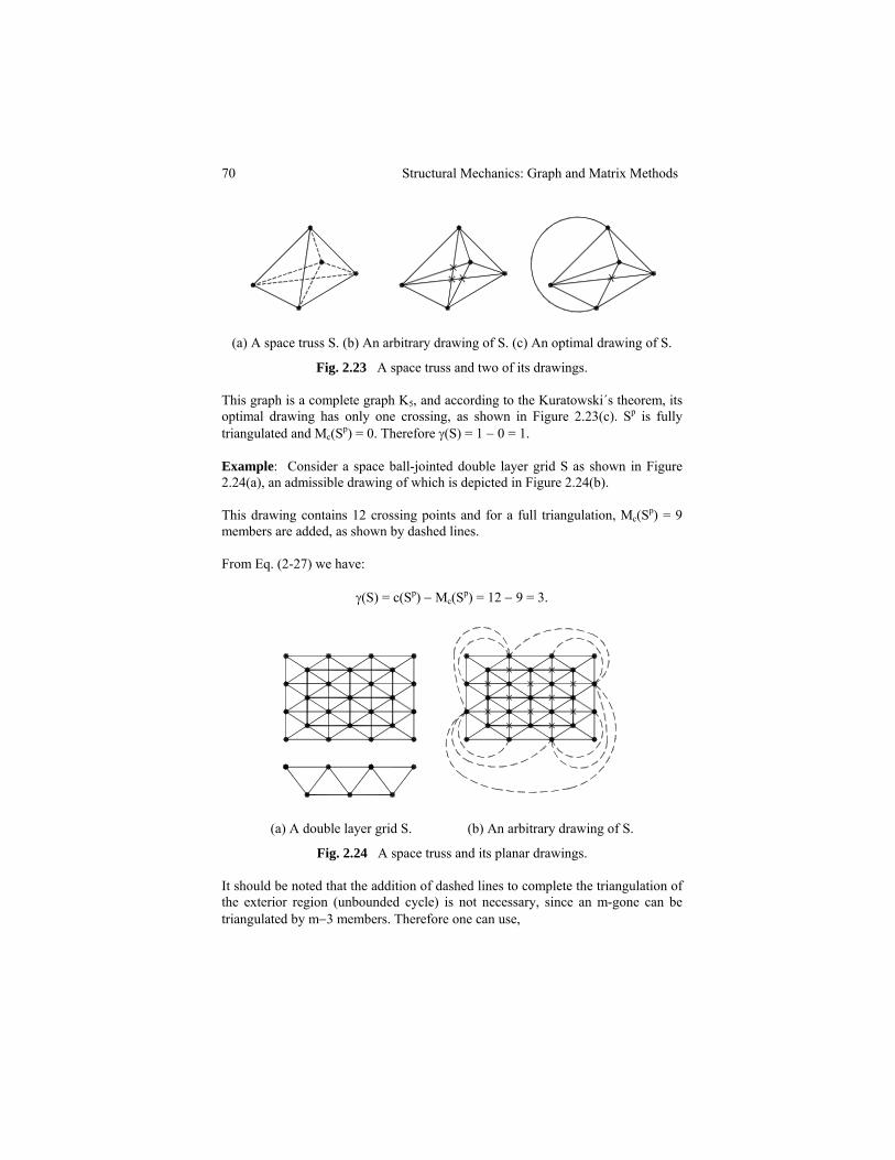
Example: S is a simple ball-jointed truss as shown in Figure 2.23(a) supported in a statically determinate fashion. An arbitrary drawing in Figure 2.23(b) has c(Sp) = 3 and for a full triangulation Mc(Sp) = 2 members are required. Therefore
γ(S) = 3 − 2 = 1.
70 Structural Mechanics: Graph and Matrix Methods
(a) A space truss S. (b) An arbitrary drawing of S. (c) An optimal drawing of S.
Fig. 2.23 A space truss and two of its drawings.
This graph is a complete graph K5, and according to the Kuratowski´s theorem, its optimal drawing has only one crossing, as shown in Figure 2.23(c). Sp is fully triangulated and Mc(Sp) = 0. Therefore γ(S) = 1 − 0 = 1.
Example: Consider a space ball-jointed double layer grid S as shown in Figure 2.24(a), an admissible drawing of which is depicted in Figure 2.24(b).
This drawing contains 12 crossing points and for a full triangulation, Mc(Sp) = 9 members are added, as shown by dashed lines.
From Eq. (2-27) we have:
γ(S) = c(Sp) − Mc(Sp) = 12 − 9 = 3.
(a) A double layer grid S. (b) An arbitrary drawing of S.
Fig. 2.24 A space truss and its planar drawings.
It should be noted that the addition of dashed lines to complete the triangulation of the exterior region (unbounded cycle) is not necessary, since an m-gone can be triangulated by m−3 members. Therefore one can use,
CHAPTER 2 Topological Properties of Skeletal Structures 71
γ(S) = c(Sp) − ,3m)(SM pc +− (2-29)
where )(SM pc is the number of members required for a full triangulation of
bounded regions.
2.6.4 COMPARISON OF CLASSICAL AND TOPOLOGICAL FORMULAE
In this section the classical and topological formulae for determining the DSI of skeletal structures are summarized as in Table 2.2. Though the classical formulae look more simple than the topological ones, the latter offer more information. Some of the advantages are as follows:
1. The number of counting for topological formulae is far less than those of the classical ones.
2. Topological formulae provide insight into the connectivity of structures and give additional information on the distribution of the indeterminacy in the vicinity of the structures.
3. The methods incorporated in the derivation of the topological formulae may be used in the study of other properties associated with graph models.
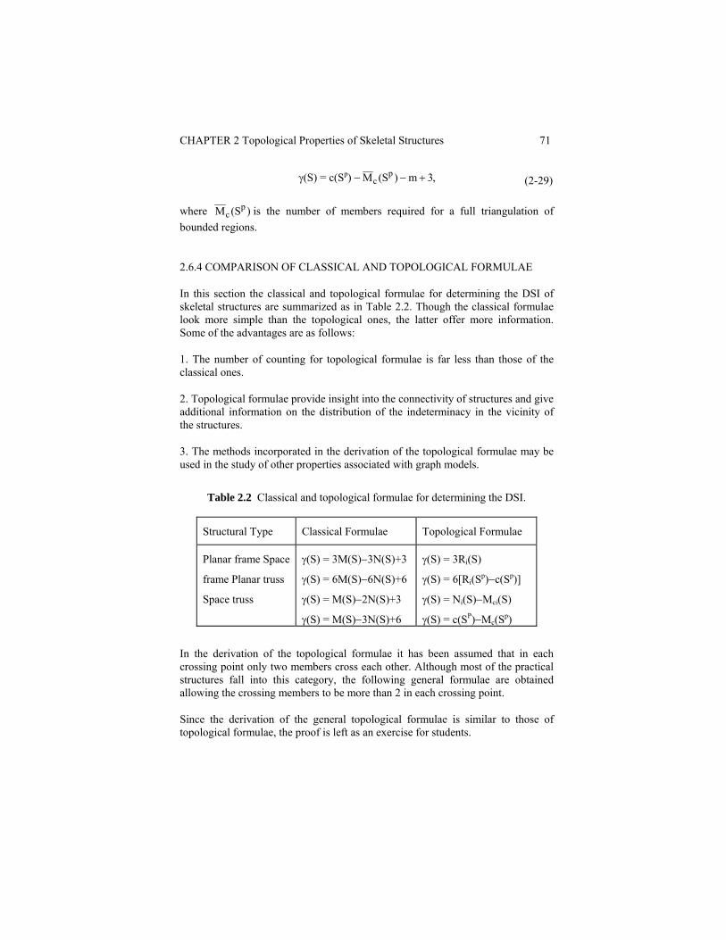
Table 2.2 Classical and topological formulae for determining the DSI.
Structural Type Classical Formulae Topological Formulae
Planar frame Space
frame Planar truss
Space truss
γ(S) = 3M(S)−3N(S)+3
γ(S) = 6M(S)−6N(S)+6
γ(S) = M(S)−2N(S)+3
γ(S) = M(S)−3N(S)+6
γ(S) = 3Ri(S)
γ(S) = 6[Ri(Sp)−c(Sp)]
γ(S) = Ni(S)−Mci(S)
γ(S) = c(SP)−Mc(Sp)
In the derivation of the topological formulae it has been assumed that in each crossing point only two members cross each other. Although most of the practical structures fall into this category, the following general formulae are obtained allowing the crossing members to be more than 2 in each crossing point.
Since the derivation of the general topological formulae is similar to those of topological formulae, the proof is left as an exercise for students.
72 Structural Mechanics: Graph and Matrix Methods
Three examples are given for illustrating the applications:
For planar frames: ])S(C)1j()S(R[ 3)S(k
2j
pjpi ∑
=−−=γ . (2-30)
For space frames: ])S(C)1j()S(R[ 6)S(k
2j
pjpi ∑
=−−=γ . (2-31)
For planar trusses: ∑=
−−−=γk
2j
pjpci
pi )S(C)2j()S(M)S(N)S( . (2-32)
For space trusses: )S(M)S(C)j3()S( pc
k
2j
pj −−=γ ∑=
. (2-33)
In the above formulae, Cj(Sp) is the number of points with j members crossing at these points.
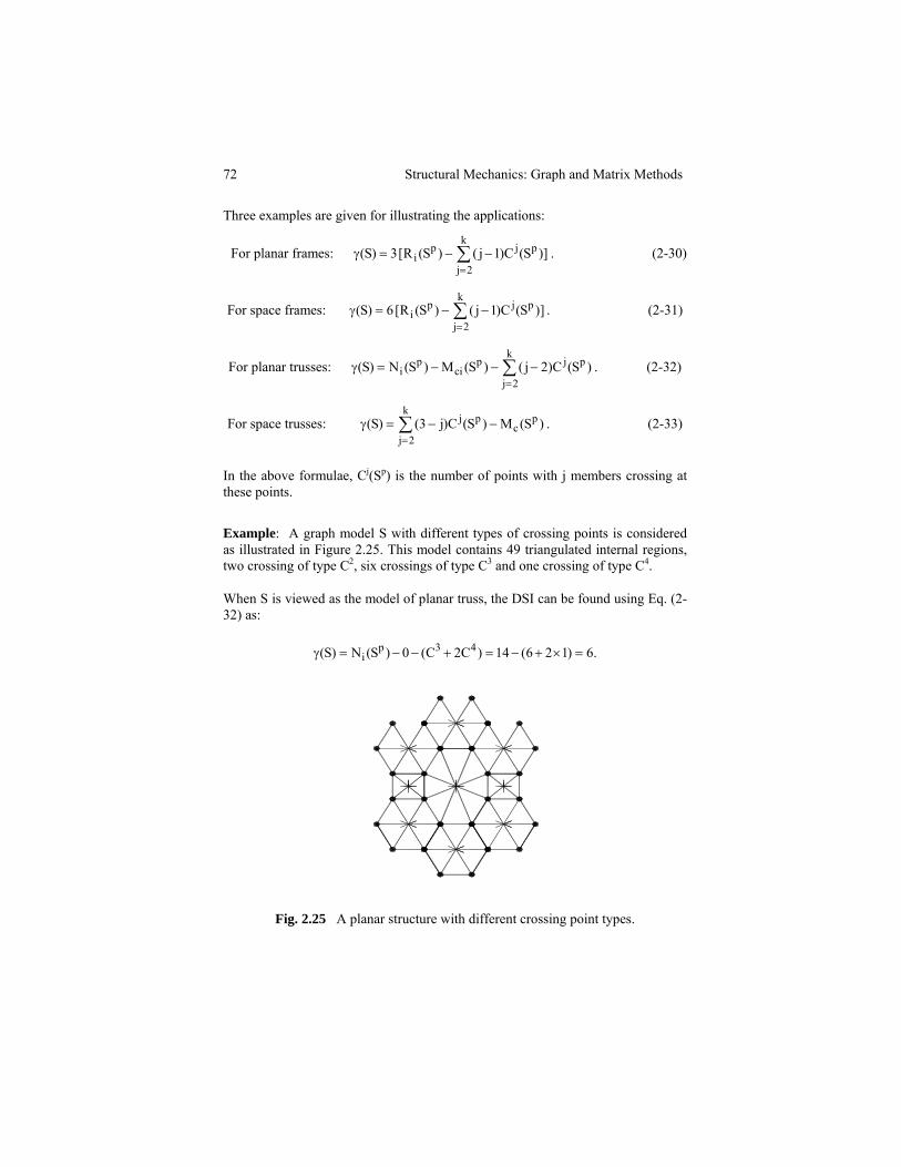
Example: A graph model S with different types of crossing points is considered as illustrated in Figure 2.25. This model contains 49 triangulated internal regions, two crossing of type C2, six crossings of type C3 and one crossing of type C4.
When S is viewed as the model of planar truss, the DSI can be found using Eq. (2-32) as:
.6)126(14)C2C(0)S(N)S( 43pi =×+−=+−−=γ
Fig. 2.25 A planar structure with different crossing point types.
CHAPTER 2 Topological Properties of Skeletal Structures 73
For S being a planar frame, the DSI is calculated using Eq. (2-30) as:
.96)]13622(49[3)]C3C2C()S(R[ 3)S( 432pi =×+×+−=++−=γ
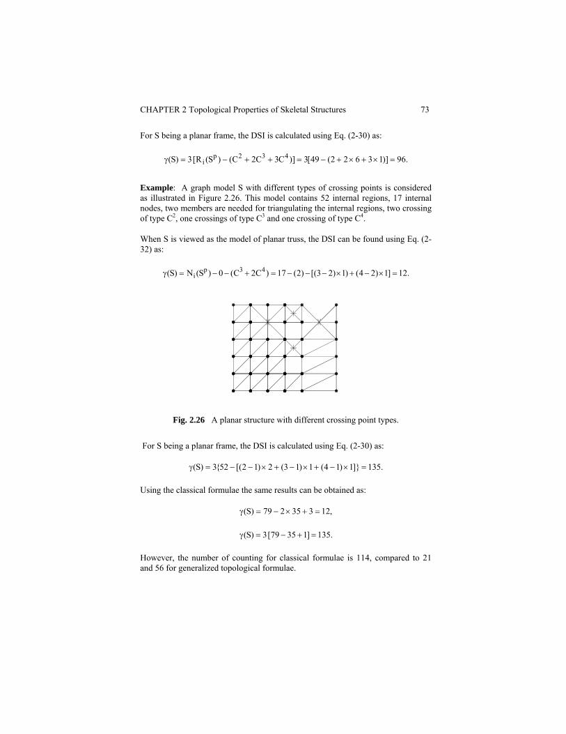
Example: A graph model S with different types of crossing points is considered as illustrated in Figure 2.26. This model contains 52 internal regions, 17 internal nodes, two members are needed for triangulating the internal regions, two crossing of type C2, one crossings of type C3 and one crossing of type C4.
When S is viewed as the model of planar truss, the DSI can be found using Eq. (2- 32) as:
.12]1)24()1)23[()2(17)C2C(0)S(N)S( 43pi =×−+×−−−=+−−=γ
Fig. 2.26 A planar structure with different crossing point types.
For S being a planar frame, the DSI is calculated using Eq. (2-30) as:
.135]}1)14(1)13(2)12[(52{3)S( =×−+×−+×−−=γ
Using the classical formulae the same results can be obtained as:
,12335279)S( =+×−=γ
.135]13579[ 3)S( =+−=γ
However, the number of counting for classical formulae is 114, compared to 21 and 56 for generalized topological formulae.
74 Structural Mechanics: Graph and Matrix Methods
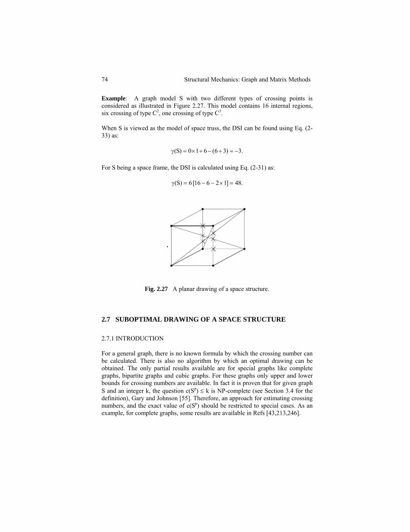
Example: A graph model S with two different types of crossing points is considered as illustrated in Figure 2.27. This model contains 16 internal regions, six crossing of type C2, one crossing of type C3.
When S is viewed as the model of space truss, the DSI can be found using Eq. (2-33) as:
.3)36(610)S( −=+−+×=γ
For S being a space frame, the DSI is calculated using Eq. (2-31) as:
.48]12616[ 6)S( =×−−=γ
Fig. 2.27 A planar drawing of a space structure.
2.7 SUBOPTIMAL DRAWING OF A SPACE STRUCTURE
2.7.1 INTRODUCTION
For a general graph, there is no known formula by which the crossing number can be calculated. There is also no algorithm by which an optimal drawing can be obtained. The only partial results available are for special graphs like complete graphs, bipartite graphs and cubic graphs. For these graphs only upper and lower bounds for crossing numbers are available. In fact it is proven that for given graph S and an integer k, the question c(Sp) ≤ k is NP-complete (see Section 3.4 for the definition), Gary and Johnson [55]. Therefore, an approach for estimating crossing numbers, and the exact value of c(Sp) should be restricted to special cases. As an example, for complete graphs, some results are available in Refs [43,213,246].
CHAPTER 2 Topological Properties of Skeletal Structures 75
Two theorems of the previous subsections provide useful lower bounds for the crossing number of space structures, and lead to the design of an efficient algorithm for suboptimal drawings of a general graph.
Corollary 1: The statical indeterminacy γ(S) of a ball-jointed space truss S, is a lower bound to the crossing number of S.
Consider Eq. (2-27) as,
γ(S) = c(Sp) − Mc(Sp),
and rearrange its terms as:
c(Sp) = γ(S) + Mc(Sp). (2-34)
Since Mc(Sp) ≥ 0, therefore:
c(Sp) ≥ γ(S).
Hence γ(S) is a lower bound for c(Sp).
From Eq. (2-34) it follows that:
Min c(Sp) ↔ Min Mc(Sp). (2-35)
Corollary 2: The crossing number of a graph is related to its Betti number by:
c(Sp) = Ri(Sp) − b1(S). (2-36)
This is obvious from Eq. (2-25) if its terms are rearranged. Therefore, to minimize c(Sp) one should minimize the number of internal regions of its planar drawing, i.e.
Min c(Sp) ↔ Min Ri(Sp). (2-37)
Based on the above results, an intuitive algorithm can be designed for suboptimal drawing. However, for an automatic drawing an algebraic graph theory method is developed [129] as presented in the following section.
2.7.2 AUTOMATIC DRAWING OF A SPACE STRUCTURE
Definitions: A graph can efficiently be represented by its member-node list, and the adjacency matrix of the graph can easily be constructed. Consider a graph with 10 nodes and 19 members, having the following adjacency matrix:
76 Structural Mechanics: Graph and Matrix Methods
,
111sym
11111
11111
111111
10987654321
10987654321
⎥⎥⎥⎥⎥⎥⎥⎥⎥⎥⎥⎥⎥⎥⎥⎥⎥
⎦
⎤
⎢⎢⎢⎢⎢⎢⎢⎢⎢⎢⎢⎢⎢⎢⎢⎢⎢
⎣
⎡
••
••
••
••
••
=A
(2-38)
where only non-zero entries are shown for clarity. When drawing this graph, the nodes are placed on a straight line and the members are placed at the top and bottom in a random manner. Members at the top and bottom of this line are identified by +1 and −1, respectively, resulting in a new matrix A*.
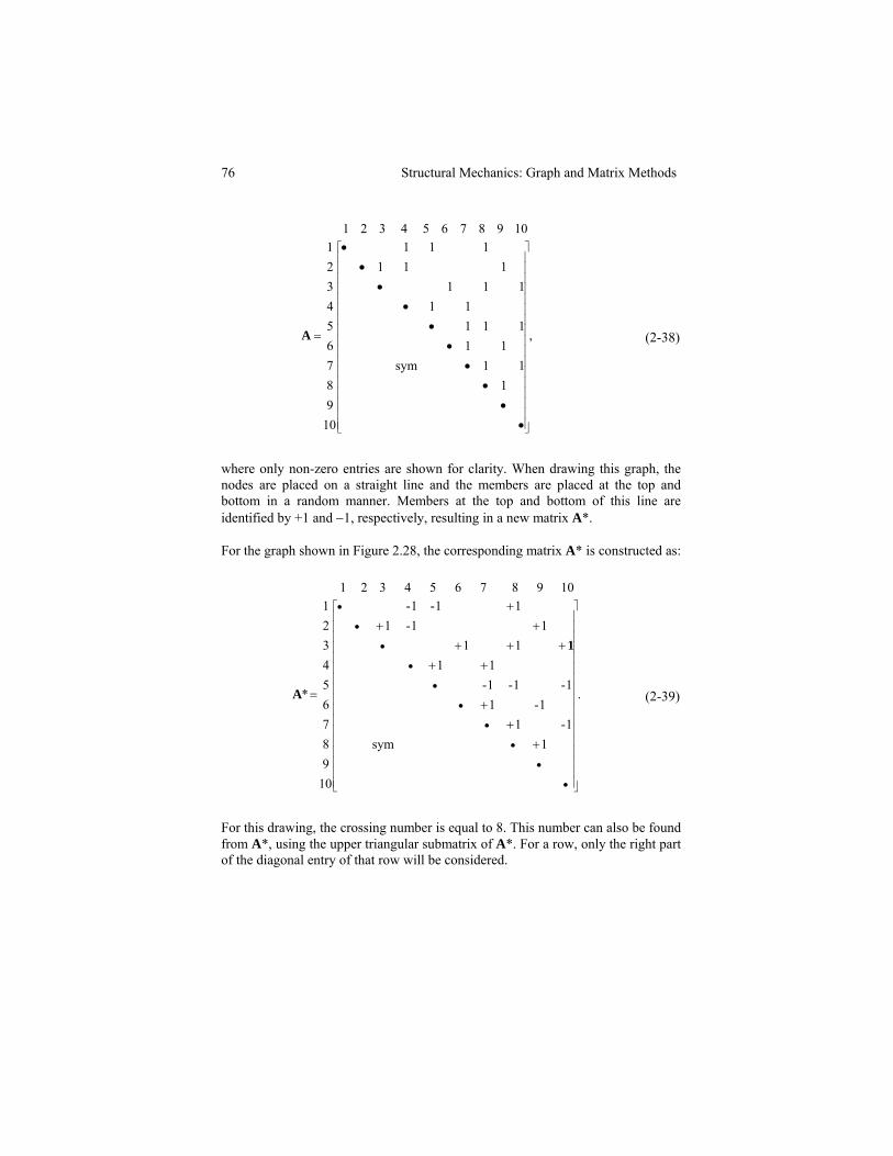
For the graph shown in Figure 2.28, the corresponding matrix A* is constructed as:
.
1sym1-1
1-11-1-1-
1111
11-111-1-
10987654321
*
10 9 8 7 6 5 4 32 1
⎥⎥⎥⎥⎥⎥⎥⎥⎥⎥⎥⎥⎥⎥⎥⎥⎥
⎦
⎤
⎢⎢⎢⎢⎢⎢⎢⎢⎢⎢⎢⎢⎢⎢⎢⎢⎢
⎣
⎡
•
•
•
•
•
•
•
•
•
•
++
+
+++++
+++
=
1
A
(2-39)
For this drawing, the crossing number is equal to 8. This number can also be found from A*, using the upper triangular submatrix of A*. For a row, only the right part of the diagonal entry of that row will be considered.
CHAPTER 2 Topological Properties of Skeletal Structures 77
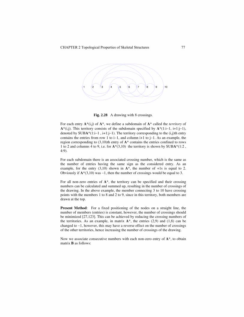
1 2 3 4 5 6 7 8 9 10
Fig. 2.28 A drawing with 8 crossings.
For each entry A*(i,j) of A*, we define a subdomain of A* called the territory of A*(i,j). This territory consists of the subdomain specified by A*(1:i−1, i+1:j−1), denoted by SUBA*(1:i−1 , i+1:j−1). The territory corresponding to the (i,j)th entry contains the entries from row 1 to i−1, and column i+1 to j−1. As an example, the region corresponding to (3,10)th entry of A* contains the entries confined to rows 1 to 2 and columns 4 to 9, i.e. for A*(3,10) the territory is shown by SUBA*(1:2 , 4:9).
For each subdomain there is an associated crossing number, which is the same as the number of entries having the same sign as the considered entry. As an example, for the entry (3,10) shown in A*, the number of +1s is equal to 2. Obviously if A*(3,10) was −1, then the number of crossings would be equal to 3.
For all non-zero entries of A*, the territory can be specified and their crossing numbers can be calculated and summed up, resulting in the number of crossings of the drawing. In the above example, the member connecting 3 to 10 have crossing points with the members 1 to 8 and 2 to 9, since in this territory, both members are drawn at the top.
Present Method: For a fixed positioning of the nodes on a straight line, the number of members (entries) is constant, however, the number of crossings should be minimized [27,123]. This can be achieved by reducing the crossing numbers of the territories. As an example, in matrix A*, the entries (2,9) and (1,8) can be changed to −1, however, this may have a reverse effect on the number of crossings of the other territories, hence increasing the number of crossings of the drawing.
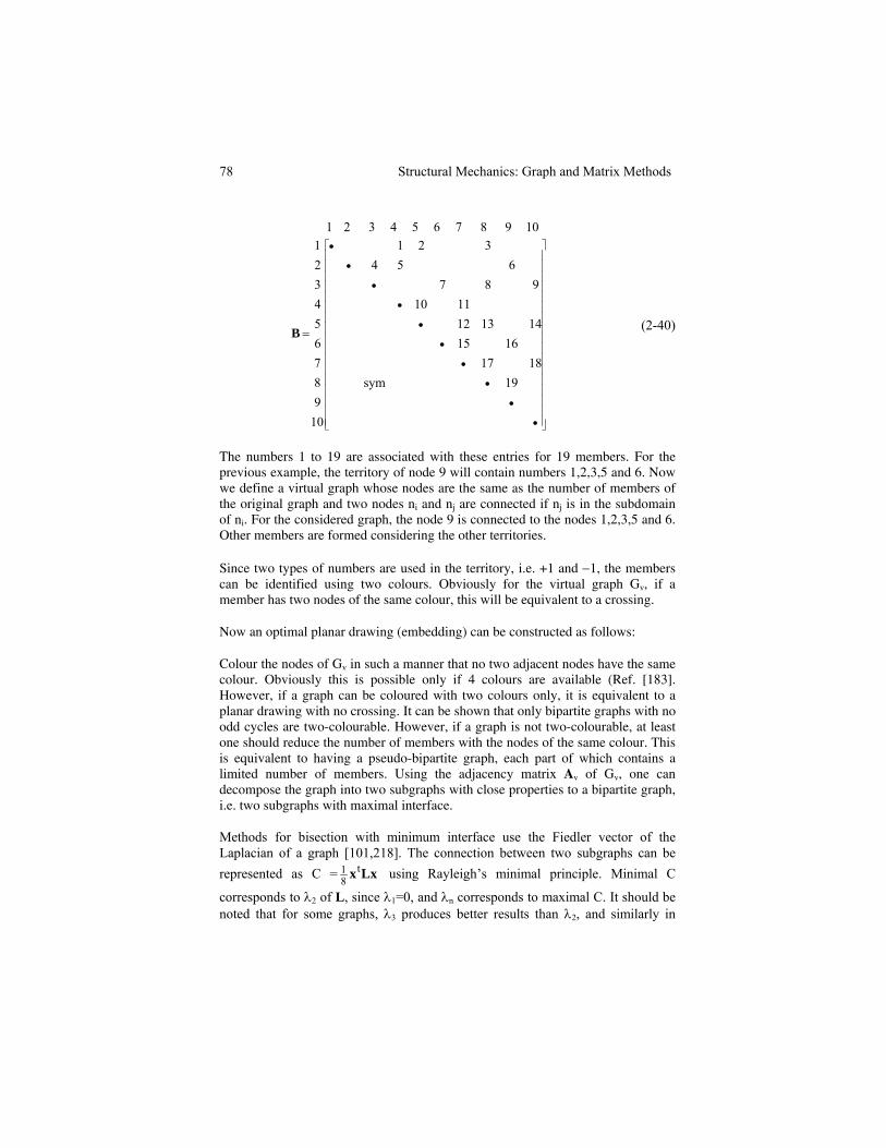
Now we associate consecutive numbers with each non-zero entry of A*, to obtain matrix B as follows:
78 Structural Mechanics: Graph and Matrix Methods
⎥⎥⎥⎥⎥⎥⎥⎥⎥⎥⎥⎥⎥⎥⎥⎥⎥
⎦
⎤
⎢⎢⎢⎢⎢⎢⎢⎢⎢⎢⎢⎢⎢⎢⎢⎢⎢
⎣
⎡
•
•
•
•
•
•
•
•
•
•
=
19sym1817
1615141312
1110987
654321
10987654321
109 8 76543 21
B
(2-40)
The numbers 1 to 19 are associated with these entries for 19 members. For the previous example, the territory of node 9 will contain numbers 1,2,3,5 and 6. Now we define a virtual graph whose nodes are the same as the number of members of the original graph and two nodes ni and nj are connected if nj is in the subdomain of ni. For the considered graph, the node 9 is connected to the nodes 1,2,3,5 and 6. Other members are formed considering the other territories.
Since two types of numbers are used in the territory, i.e. +1 and −1, the members can be identified using two colours. Obviously for the virtual graph Gv, if a member has two nodes of the same colour, this will be equivalent to a crossing.
Now an optimal planar drawing (embedding) can be constructed as follows:
Colour the nodes of Gv in such a manner that no two adjacent nodes have the same colour. Obviously this is possible only if 4 colours are available (Ref. [183]. However, if a graph can be coloured with two colours only, it is equivalent to a planar drawing with no crossing. It can be shown that only bipartite graphs with no odd cycles are two-colourable. However, if a graph is not two-colourable, at least one should reduce the number of members with the nodes of the same colour. This is equivalent to having a pseudo-bipartite graph, each part of which contains a limited number of members. Using the adjacency matrix Av of Gv, one can decompose the graph into two subgraphs with close properties to a bipartite graph, i.e. two subgraphs with maximal interface. Methods for bisection with minimum interface use the Fiedler vector of the Laplacian of a graph [101,218]. The connection between two subgraphs can be represented as C = Lxxt
81 using Rayleigh’s minimal principle. Minimal C
corresponds to λ2 of L, since λ1=0, and λn corresponds to maximal C. It should be noted that for some graphs, λ3 produces better results than λ2, and similarly in
CHAPTER 2 Topological Properties of Skeletal Structures 79
maximal case, λn-1 might perform better than λn. This is observed for planarization of K7.
After calculating λmax or λn, the corresponding eigenvectors can be found. Here instead of ordering and partitioning as in φ2, the positive or negative nature of φn is considered and replaced by +1 and −1. These values specify the members of graphs on the top and bottom of the straight line, respectively. Once A* is formed, the number of crossings can easily be evaluated.
The problem of bisection can be formulated in the form of a maximal-flow or Minimum-cut problem, Lawler [157,32], and there are other approximate algorithms concerning this problem, Ref. [73].
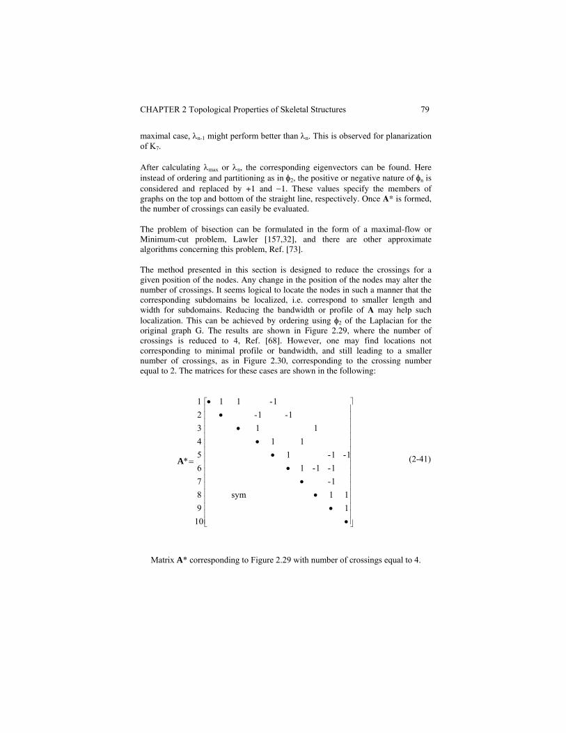
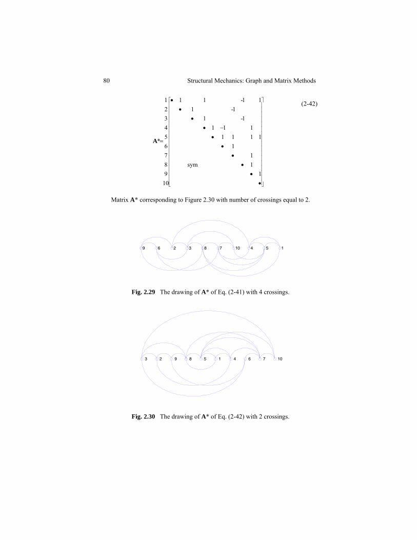
The method presented in this section is designed to reduce the crossings for a given position of the nodes. Any change in the position of the nodes may alter the number of crossings. It seems logical to locate the nodes in such a manner that the corresponding subdomains be localized, i.e. correspond to smaller length and width for subdomains. Reducing the bandwidth or profile of A may help such localization. This can be achieved by ordering using φ2 of the Laplacian for the original graph G. The results are shown in Figure 2.29, where the number of crossings is reduced to 4, Ref. [68]. However, one may find locations not corresponding to minimal profile or bandwidth, and still leading to a smaller number of crossings, as in Figure 2.30, corresponding to the crossing number equal to 2. The matrices for these cases are shown in the following:
⎥⎥⎥⎥⎥⎥⎥⎥⎥⎥⎥⎥⎥⎥⎥⎥⎥
⎦
⎤
⎢⎢⎢⎢⎢⎢⎢⎢⎢⎢⎢⎢⎢⎢⎢⎢⎢
⎣
⎡
••
••
••
••
••
=
111sym
1-1-1-1
1-1-111
111-1-
1-11
10987654321
*A
(2-41)
Matrix A* corresponding to Figure 2.29 with number of crossings equal to 4.
80 Structural Mechanics: Graph and Matrix Methods
⎥⎥⎥⎥⎥⎥⎥⎥⎥⎥⎥⎥⎥⎥⎥⎥⎥
⎦
⎤
⎢⎢⎢⎢⎢⎢⎢⎢⎢⎢⎢⎢⎢⎢⎢⎢⎢
⎣
⎡
••
••
••
−••
••
=
11sym1
11111
1111-1
1-111-11
10987654321
*A
(2-42)
Matrix A* corresponding to Figure 2.30 with number of crossings equal to 2.
9 6 2 3 8 7 10 4 5 1
Fig. 2.29 The drawing of A* of Eq. (2-41) with 4 crossings.
3 2 9 8 5 1 4 6 7 10
Fig. 2.30 The drawing of A* of Eq. (2-42) with 2 crossings.
CHAPTER 2 Topological Properties of Skeletal Structures 81
It can be seen that the matrix in Figure 2.30 is not well structured, however, the corresponding crossing number has the least magnitude.
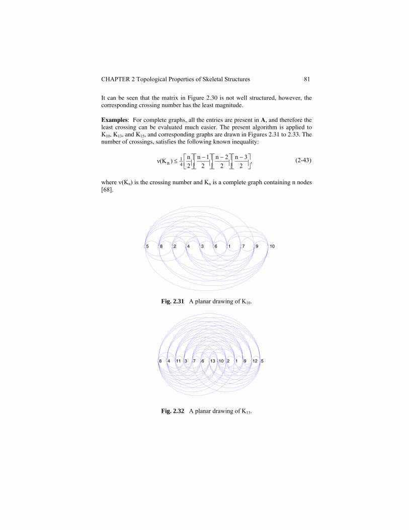
Examples: For complete graphs, all the entries are present in A, and therefore the least crossing can be evaluated much easier. The present algorithm is applied to K10, K13, and K15, and corresponding graphs are drawn in Figures 2.31 to 2.33. The number of crossings, satisfies the following known inequality:
,2
3n2
2n2
1n2n)ν(K 4
1n ⎥⎦
⎤⎢⎣⎡ −
⎥⎦⎤
⎢⎣⎡ −
⎥⎦⎤
⎢⎣⎡ −
⎥⎦⎤
⎢⎣⎡≤ (2-43)
where ν(Kn) is the crossing number and Kn is a complete graph containing n nodes [68].
5 8 2 4 3 6 1 7 9 10
Fig. 2.31 A planar drawing of K10.
8 4 11 3 7 6 13 10 2 1 9 12 5
Fig. 2.32 A planar drawing of K13.
82 Structural Mechanics: Graph and Matrix Methods
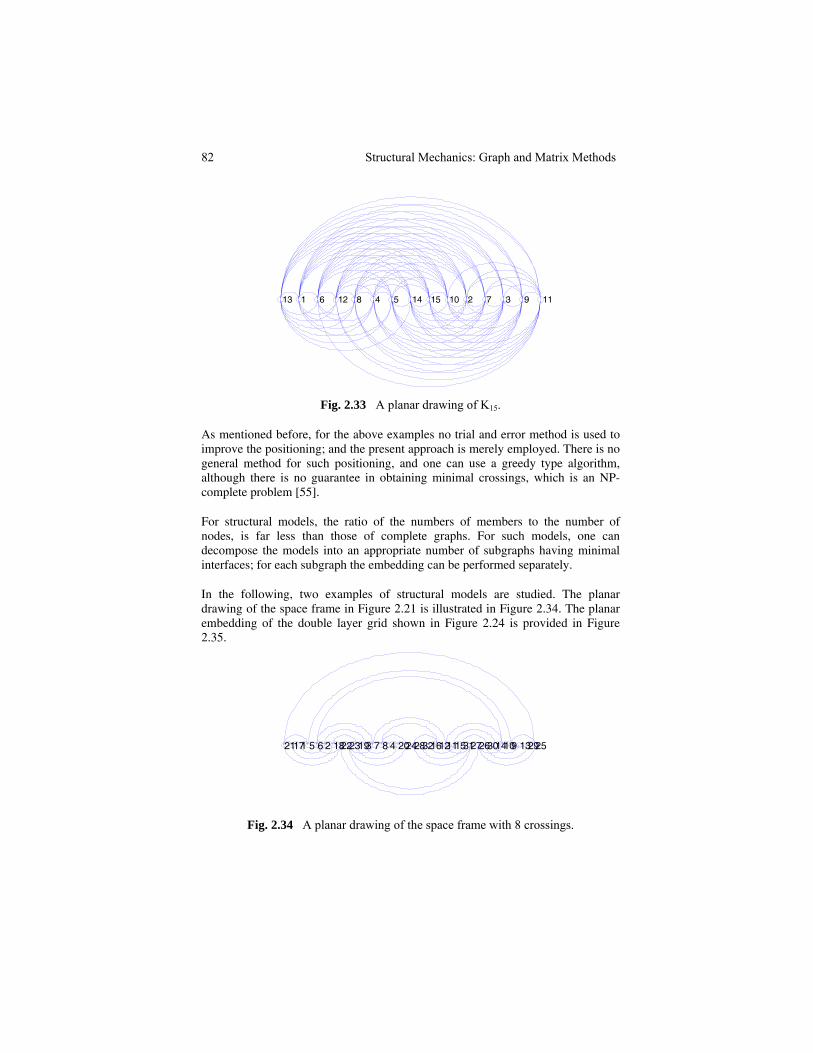
13 1 6 12 8 4 5 14 15 10 2 7 3 9 11
Fig. 2.33 A planar drawing of K15.
As mentioned before, for the above examples no trial and error method is used to improve the positioning; and the present approach is merely employed. There is no general method for such positioning, and one can use a greedy type algorithm, although there is no guarantee in obtaining minimal crossings, which is an NP-complete problem [55].
For structural models, the ratio of the numbers of members to the number of nodes, is far less than those of complete graphs. For such models, one can decompose the models into an appropriate number of subgraphs having minimal interfaces; for each subgraph the embedding can be performed separately.
In the following, two examples of structural models are studied. The planar drawing of the space frame in Figure 2.21 is illustrated in Figure 2.34. The planar embedding of the double layer grid shown in Figure 2.24 is provided in Figure 2.35.
21 17 1 5 6 2 182223193 7 8 4 20242832161211153127263014109 132925
Fig. 2.34 A planar drawing of the space frame with 8 crossings.
CHAPTER 2 Topological Properties of Skeletal Structures 83
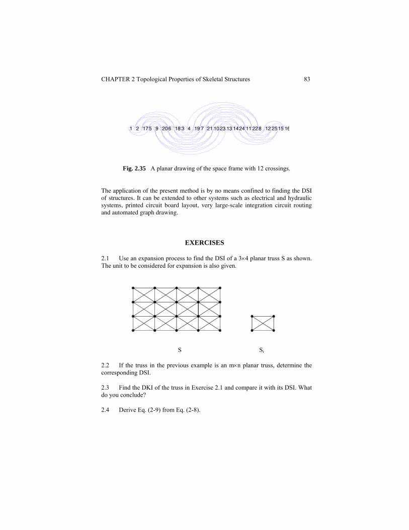
1 2 175 9 206 18 3 4 19 7 21 1023 13 1424 11 228 12 2515 16
Fig. 2.35 A planar drawing of the space frame with 12 crossings.
The application of the present method is by no means confined to finding the DSI of structures. It can be extended to other systems such as electrical and hydraulic systems, printed circuit board layout, very large-scale integration circuit routing and automated graph drawing.
EXERCISES
2.1 Use an expansion process to find the DSI of a 3×4 planar truss S as shown. The unit to be considered for expansion is also given.
S Si
2.2 If the truss in the previous example is an m×n planar truss, determine the corresponding DSI.
2.3 Find the DKI of the truss in Exercise 2.1 and compare it with its DSI. What do you conclude?
2.4 Derive Eq. (2-9) from Eq. (2-8).
84 Structural Mechanics: Graph and Matrix Methods
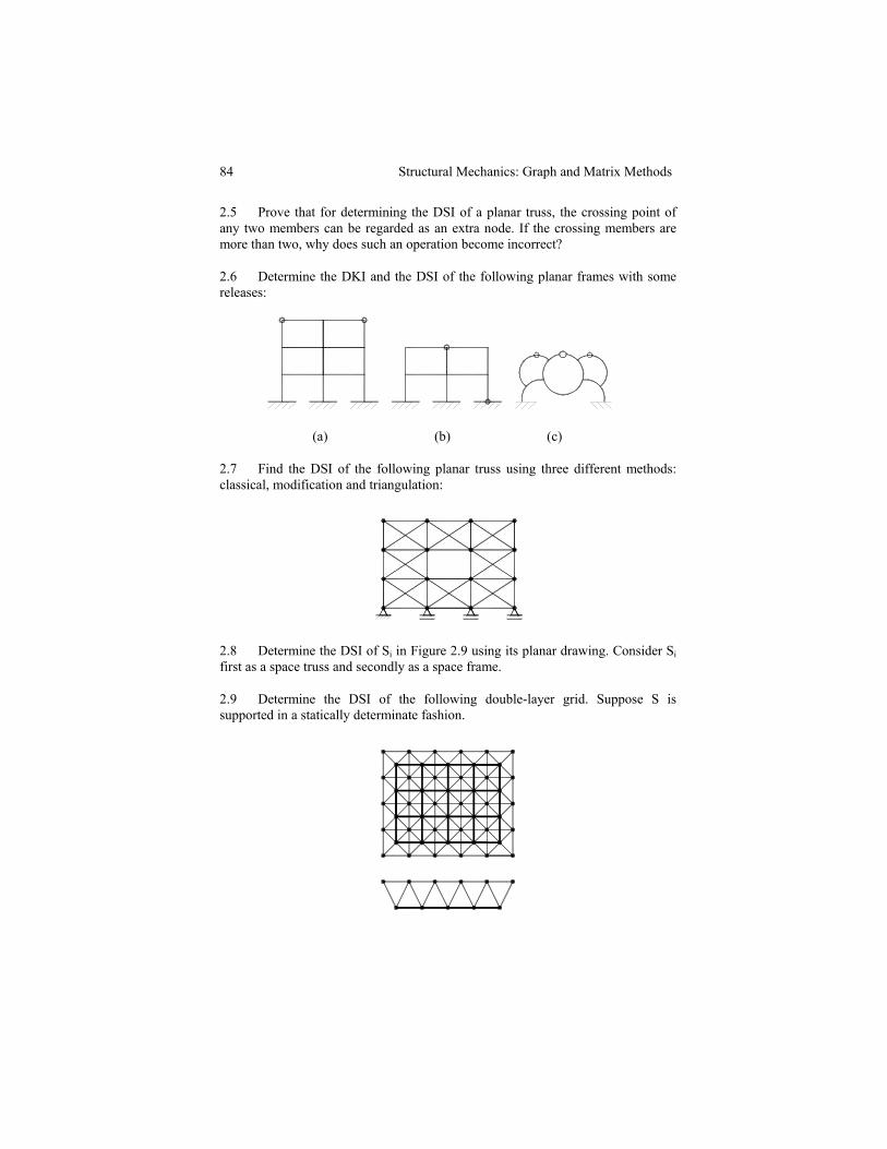
2.5 Prove that for determining the DSI of a planar truss, the crossing point of any two members can be regarded as an extra node. If the crossing members are more than two, why does such an operation become incorrect?
2.6 Determine the DKI and the DSI of the following planar frames with some releases:
(a) (b) (c)
2.7 Find the DSI of the following planar truss using three different methods: classical, modification and triangulation:
2.8 Determine the DSI of Si in Figure 2.9 using its planar drawing. Consider Si first as a space truss and secondly as a space frame.
2.9 Determine the DSI of the following double-layer grid. Suppose S is supported in a statically determinate fashion.