Topics on Beam Dynamics at SPring-8 Storage Ring

K. Soutome (JASRI/SPring-8)

on behalf of JASRI Accelerator Division

SSRF(Feb. 16, 2009)

Topics 1) Sextupole Optimization for the Ring with LSS 2) Short Bunch Generation by Low-Alpha Operation 3) What we are discussing on Machine Upgrading

SX Optimization for LSS

8GeV Electron Storage Ring Circumference: 1436m Beam Current: 100mA Lattice: Double-Bend with four 30m-LSSs Natural Emittance: 6.6nmrad　(Achromat) 3.4nmrad　(Non-Achromat)

SX Optimization for LSS

Ring with 48-Cell Structure

[ (Normal Cell) × 9 + (Matching Cell) + (Long Straight) + (Matching Cell) ] × 4

Cell Length: 30m

SX Optimization for LSS

We started beam commissioning with this optics. "24-Fold Symmetric"

0

10

20

30

40

0

0.5

1

1.5

2

0 20 40 60 80 100 120

Bet

atro

n Fu

nctio

n β

[m]

Dispersion Function η [m

]

Path Length [m]

βxβy

ηx

Hybrid Optics with 6.9nmrad1997/3 - 1999/7

Missing-B

4/48 of Ring

SX Optimization for LSS

HHLV: High-Horizontal and Low-Vertical beta "48-Fold Symmetric"

0

10

20

30

40

0

0.5

1

1.5

2

0 20 40 60 80 100 120

Bet

atro

n Fu

nctio

n β

[m]

Dispersion Function η [m

]

Path Length [m]

βxβy

ηx

HHLV Optics with 6.3nmrad1999/9 - 2000/74/48 of

Ring

SX Optimization for LSS

"4-Fold Symmetric" strictly, but owing to matching condition "36-Fold Symmetric" approximately (36=48-3×4)

4/48 of Ring

0

10

20

30

40

50

60

0

0.5

1

1.5

2

2.5

3

0 20 40 60 80 100 120

Bet

atro

n Fu

nctio

n β

[m]

Dispersion Function η [m

]

Path Length [m]

βxβy

ηx

Achromat Optics with 6.6nmrad2000/8 - 2002/112003/10 - 2005/9

LSS

SX Optimization for LSS

Emittance was reduced by dispersion leakage. "4-Fold Symmetric" approximately

4/48 of Ring

0

10

20

30

40

50

60

0

0.5

1

1.5

2

2.5

3

0 20 40 60 80 100 120

Bet

atro

n Fu

nctio

n β

[m]

Dispersion Function η [m

]

Path Length [m]

βxβy

ηx

Low-Emittance Optics with 3.4nmrad2002/11 - 2003/102005/9 -

LSS

SX Optimization for LSS Matching Condition

(1) Betatron Phase Matching Δψx=4π, Δψy=2π For on-momentum electrons this makes the matching section transparent and the dynamic aperture is kept large.

(2) Local Chromaticity Correction For off-momentum electrons the above condition does not hold due to non-zero chromaticity, and sextupoles (SFL) are weakly excited to correct local chromaticity in the horizontal direction.

0

10

20

30

40

50

60

0

0.1

0.2

0.3

0.4

0.5

0.6

0 30 60 90

β [m

] η[m]

s [m]

βx

βy

ηx

SFL SFL

Matching Section

Horizontal chromaticity is corrected to keep high injection efficiency and long Touschek beam lifetime.

H.Tanaka, et al., NIMA486(2002)521

Only SFL-sextupoles are used in matchign section.

SX Optimization for LSS Matching Condition + Counter-Sextupoles

(3) Counter-Sextupole Non-linear kick by SFL can be canceled by another sextupole located nπ apart from SFL.

We actually adopted triplet scheme where three sextupoles are used to take account of the vertical direction too.

K.Soutome, et al., Proc. EPAC08, p.3149

Δψ = π

Kick by SFL

s

SFL SCT

Counter-Kickby SCT

x

beam

SX Optimization for LSS

0

10

20

30

40

50

60

0

0.5

1

0 10 20 30 40

β[m

] Δψ/2π

s [m]

βx

βy

SFLS1L SCT

Δψx

Δψy

0

10

20

30

40

50

60

0

0.1

0.2

0.3

0.4

0.5

0.6

0 20 40 60 80

β[m

] η[m]

s [m]

βx

βy

ηx

SFL

Matching Section

SFLS1L SCT SCT S1L

Triplet Scheme

Betatron Phase Advance

SX Optimization for LSS

0

2

4

6

8

10

12

-20 -10 0 10

δ = -1%δ = 0δ = +1%

δ = -1%δ = 0δ = +1%

y [m

m]

x [mm]

with SCT without SCT

Dynamic Aperture (Cal.) Horizontal Aperture (Exp.)

Exp.: Store the beam, fire a pair of bump magnets and measure beam current after the kick.

0

0.2

0.4

0.6

0.8

1

-20 -15 -10 -5 0 5 10 15

with SCTwithout SCT

Surv

ival

Rat

e

x [mm]

Physical Aperture Limit

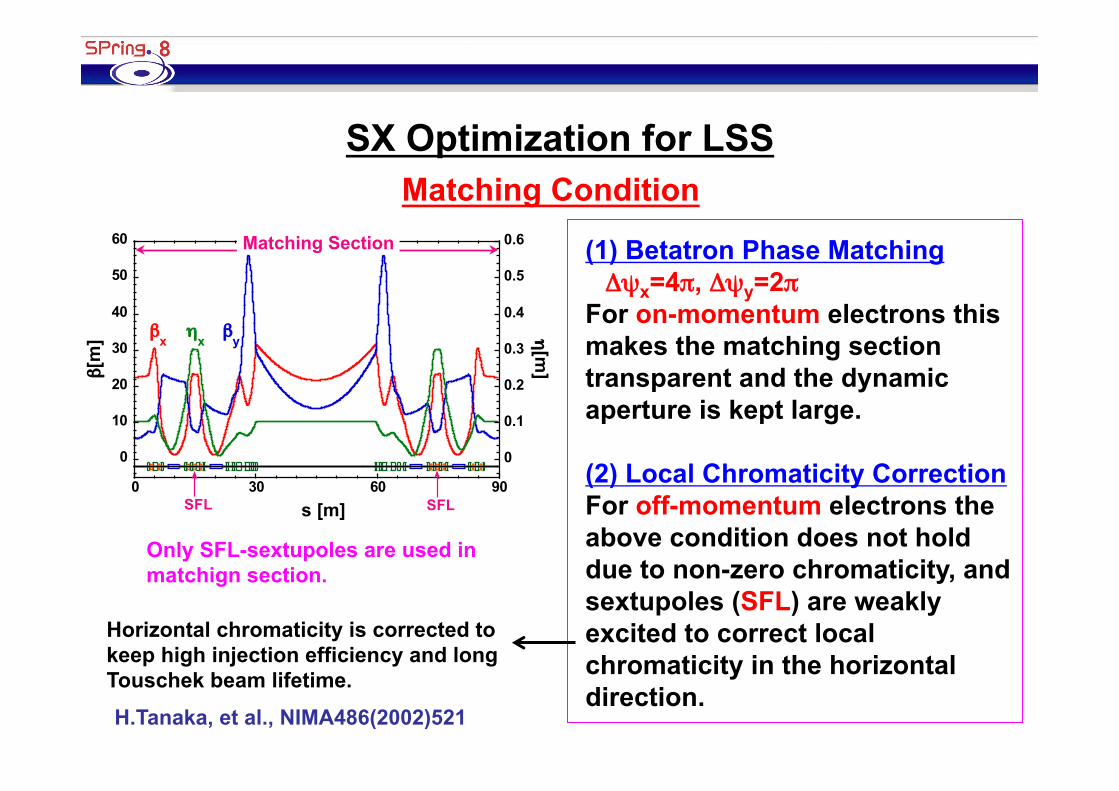
SX Optimization for LSS Non-linear behavior of betatron tune has been improved.

0.10

0.20

0.30

0.40

0.50

-0.04 -0.03 -0.02 -0.01 0 0.01 0.02 0.03

Horizontal (with SCT)Vertical (with SCT)Horizontal (w/o SCT)Vertical (w/o SCT)

Bet

atro

n Tu

ne

Δp/p

cal.

0.10

0.20

0.30

0.40

0.50

-0.04 -0.03 -0.02 -0.01 0 0.01 0.02 0.03

Horizontal (meas.)Vertical (meas.)Horizontal (cal.)Vertical (cal.)

Bet

atro

n Tu

ne

Δp/p

0

0.1

0.2

0.3

0.4

0.5

-20 -15 -10 -5 0 5 10 15

νx with SCTνy with SCTνx w/o SCTνy w/o SCT

Bet

atro

n Tu

ne

x [mm]

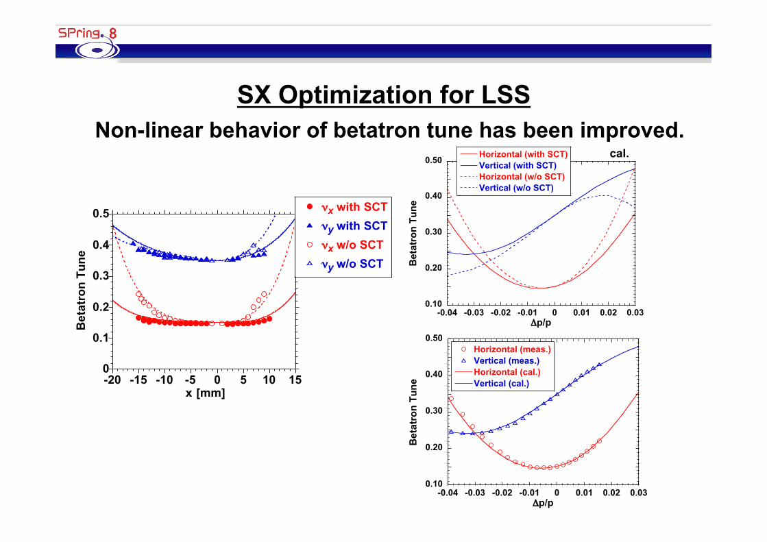
SX Optimization for LSS Non-linear dispersion has also been suppressed.

Δx = η0δ + η1δ2 + η2δ3 + ... with δ = Δp/p

-8

-6

-4

-2

0

2

4

6

8

0 200 400 600 800 1000 1200 1400

with SCTw/o SCT

η1 [m

]

s [m]

-400

-300

-200

-100

0

100

200

300

0 200 400 600 800 1000 1200 1400

η2 [m

]

s [m]

Calculation

Perturbative Formula: H.Tanaka, et al., NIM A431(1999)396; NIM A440(2000)259

SX Optimization for LSS

Comparison with experiments.

0

0.1

0.1

0.2

0.2

0.3

0.3

0.4

0 200 400 600 800 1000 1200 1400

cal.meas.

η0 [m

]

s [m]

-3

-2

-1

0

1

2

0 200 400 600 800 1000 1200 1400

η1 [m

]

s [m]

SX Optimization for LSS

-80

-60

-40

-20

0

20

40

60

0 200 400 600 800 1000 1200 1400

η2 [m

]

s [m]-800

-600

-400

-200

0

200

400

600

800

0 200 400 600 800 1000 1200 1400

η3 [m

]

s [m]

-60000

-40000

-20000

0

20000

40000

60000

0 200 400 600 800 1000 1200 1400

η4 [m

]

s [m]

SX Optimization for LSS Injection Efficiency (whit horizontal slit in transport line open)

65

70

75

80

85

90

95

100

-1 -0.5 0 0.5 1 1.5 2 2.5 3

Inje

ctio

n Ef

ficie

ncy

[%]

Δx [mm]

with SCT

w/o SCT

60

65

70

75

80

85

90

95

0 0.5 1 1.5 2

Inje

ctio

n Ef

ficie

ncy

[%]

Beam Position Δx [mm] at the End of BT Line

with SCT

w/o SCT

Exp. Cal.

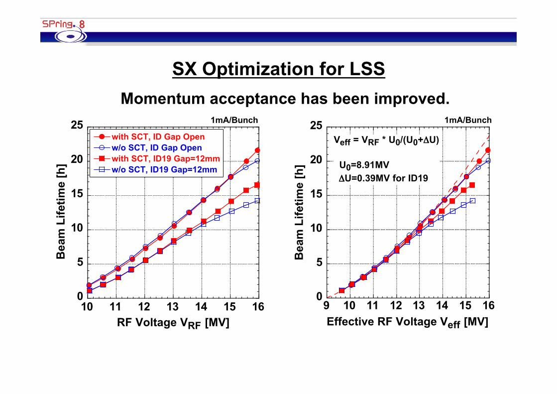
SX Optimization for LSS Momentum acceptance has been improved.

0

5

10

15

20

25

10 11 12 13 14 15 16

with SCT, ID Gap Openw/o SCT, ID Gap Openwith SCT, ID19 Gap=12mmw/o SCT, ID19 Gap=12mm

Bea

m L

ifetim

e [h

]

RF Voltage VRF [MV]

1mA/Bunch

0

5

10

15

20

25

9 10 11 12 13 14 15 16B

eam

Life

time

[h]

Effective RF Voltage Veff [MV]

Veff = VRF * U0/(U0+ΔU)

U0=8.91MV ΔU=0.39MV for ID19

1mA/Bunch

SX Optimization for LSS Application: Independent Tuning of LSS Optics It is planned to modify optics in one of four LSS's.

0

2

4

6

8

10

12

-20 -10 0 10

δ = -1%δ = 0δ = +1%

δ = -1%δ = 0δ = +1%

y [m

m]

x [mm]

with SCT w/o SCT

0

2

4

6

8

10

12

-20 -10 0 10

δ = -1%δ = 0δ = +1%

δ = -1%δ = 0δ = +1%

y [m

m]

x [mm]

with SCT w/o SCT

0

10

20

30

40

50

60

0

0.1

0.2

0.3

0.4

0.5

0.6

0 30 60 90

β [m

] η[m]

s [m]

βx βy

ηx

SCT

Matching Section

SCT SFL S1LSFLS1L

DA Before Modification

DA After Modification

After modification of LSS optics, enough DA is obtained by SCT.

SX Optimization for LSS

For local modification of optics (30m-LSS in the SPring-8 case), keeping symmetry is important, and we adopted the following:

[1] Betatron Phase Matching for on-momentum electrons to make transparent [2] Local Chromaticity Correction for off-momentum electrons to keep [1] [3] Counter-Sextupoles for cancellation of non-linear kicks due to [2]

Summary of First Topic

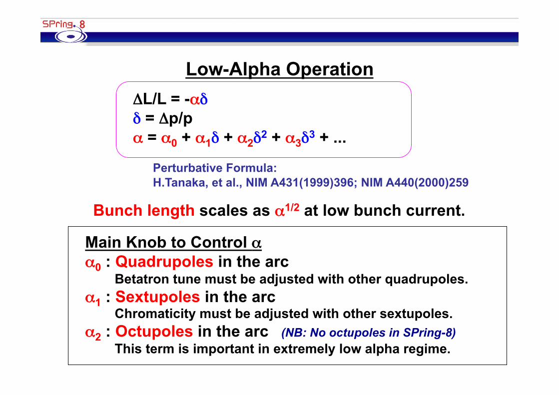
Low-Alpha Operation

Main Knob to Control α α0 : Quadrupoles in the arc Betatron tune must be adjusted with other quadrupoles. α1 : Sextupoles in the arc Chromaticity must be adjusted with other sextupoles. α2 : Octupoles in the arc (NB: No octupoles in SPring-8) This term is important in extremely low alpha regime.

ΔL/L = -αδ δ = Δp/p α = α0 + α1δ + α2δ2 + α3δ3 + ...

Perturbative Formula: H.Tanaka, et al., NIM A431(1999)396; NIM A440(2000)259

Bunch length scales as α1/2 at low bunch current.

Low-Alpha Operation

α0 = 1.68 e -4 ε = 3.4nmrad Tune: (40.15, 18.35)

1/11

Gradual Change, Tune Fixed

-100

10203040506070

-0.500.511.522.533.5

0 50 100 150 200 250 300 350

β [m

] η [m]

s [m]

βxβy

ηx

Low-Alpha Optics

-100

10203040506070

-0.500.511.522.533.5

0 50 100 150 200 250 300 350

β [m

] η [m]

s [m]

βxβy

ηx

User-Time

1/29

α0 = 1.58 e -5 ε = 24.8nmrad Tune: (39.15, 14.35)

α0 = 5.8 e -6

Ring/4 Ring/4

Low-Alpha Operation

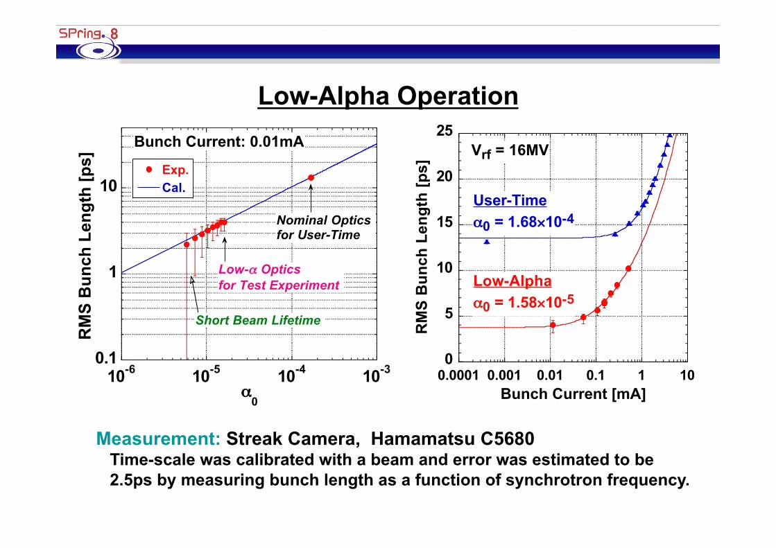
Measurement: Streak Camera, Hamamatsu C5680 Time-scale was calibrated with a beam and error was estimated to be 2.5ps by measuring bunch length as a function of synchrotron frequency.

0

5

10

15

20

25

0.0001 0.001 0.01 0.1 1 10

RM

S B

unch

Len

gth

[ps]

Bunch Current [mA]

User-Timeα0 = 1.68×10-4

Low-Alphaα0 = 1.58×10-5

Vrf = 16MV

0.1

1

10

10-6 10-5 10-4 10-3

Exp.Cal.

RM

S B

unch

Len

gth

[ps]

α0

Bunch Current: 0.01mA

Short Beam Lifetime

Nominal Opticsfor User-Time

Low-α Opticsfor Test Experiment

Low-Alpha Operation Suppression of α1 by Sextupoles for Stable Operation

0

200

400

600

800

1000

0

0.1

0.2

0.3

0.4

0.5

-50 0 50 100 150 200 250 300

RUN1

fs

νxν

y

f s [Hz]

Betatron Tune

Δfrf [Hz]

0

200

400

600

800

1000

0

0.1

0.2

0.3

0.4

0.5

-50 0 50 100 150 200 250 300

RUN2

fs

νxν

y

f s [Hz]

Betatron Tune

Δfrf [Hz]

0

200

400

600

800

1000

0

0.1

0.2

0.3

0.4

0.5

-100 -50 0 50 100 150 200 250 300

RUN3

fs

νxν

y

f s [Hz]

Betatron Tune

Δfrf [Hz]

α = α0 + α1δ

δ 0

-α0/α1

α0

Stable σδ << |α0 / α1| D.Robin, et al., Phys.Rev. E48 (1993) 2149

After setting sextupoles we can check this by observing dfsy / dfRF = 0.

Low-Alpha Operation Suppression of α2 by Octupoles (Simulation)

-3

-2

-1

0

1

2

3

-30 -20 -10 0 10 20 30 40

δ [%

]

φ - φs [deg]

-3

-2

-1

0

1

2

3

-30 -20 -10 0 10 20 30 40

δ [%

]

φ - φs [deg]

-4 10-5

-3 10-5

-2 10-5

-1 10-5

0

1 10-5

2 10-5

3 10-5

4 10-5

-0.04 -0.02 0 0.02 0.04

up to α1

up to α2

up to α4

α(δ

)

δ

α < 0 for large δ

α > 0 for small δ

α = α0 + α

1δ + α

2δ2 + ...

-4 10-5

-3 10-5

-2 10-5

-1 10-5

0

1 10-5

2 10-5

3 10-5

4 10-5

-0.04 -0.02 0 0.02 0.04

up to α1

up to α2

up to α4

α(δ

)

δ

with Octupoles

with Octupoles → calculation for temporary set of octupoles, not optimized

Alternative: operation with α0 < 0

Stable

Low-Alpha Operation

We lowered α0 down to 1/29 of nominal optics. The shortest bunch length achieved was 2ps(rms) but lifetime was short in this optics.

We carried out test experiments in the 25m-long undulator beamline under the following condition: Bunch Length: rms 4.2ps (FWHM 10ps) Bunch Current: 0.01mA Photon Intensity: 1/1000 of Nominal User-Time Filling: Several-Bunch Filling Data analysis is in progress...

Summary of Second Topic

0.1

1

10

100

0.0001 0.001 0.01 0.1 1 10

RM

S B

unch

Len

gth

[ps]

Bunch Current [mA]

α0 = 1.68×10-4

α0 = 1.58×10-5

Vrf = 16MV

α0 = 5.8×10-6

α0 = 1.3×10-6(plan)

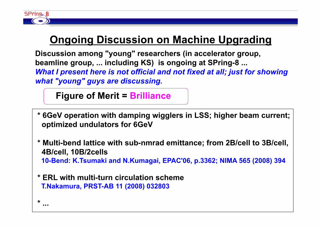
Ongoing Discussion on Machine Upgrading Discussion among "young" researchers (in accelerator group, beamline group, ... including KS) is ongoing at SPring-8 ... What I present here is not official and not fixed at all; just for showing what "young" guys are discussing.

* 6GeV operation with damping wigglers in LSS; higher beam current; optimized undulators for 6GeV

* Multi-bend lattice with sub-nmrad emittance; from 2B/cell to 3B/cell, 4B/cell, 10B/2cells 10-Bend: K.Tsumaki and N.Kumagai, EPAC'06, p.3362; NIMA 565 (2008) 394

* ERL with multi-turn circulation scheme T.Nakamura, PRST-AB 11 (2008) 032803

* ...

Figure of Merit = Brilliance

Ongoing Discussion on Machine Upgrading Example: QB Lattice with ε = 0.29nmrad (εeff = 0.33nmrad) at 8GeV

ISSUES: Emittance is calculated to be small, but ... strong quadrupoles, large chromaticity and small dispersion and hence strong sextupoles, narrow dynamic aperture, narrow momentum acceptance, short beam lifetime, no magnet-free LSS (difficult), small bore diameter, narrow chamber, limited space for BPMs and correctors, high sensitivity against errors, long dark time, cost, ...

0

10

20

30

40

0

0.05

0.1

0.15

0.2

0 5 10 15 20 25 30

βx

βy

ηx

β[m

] η [m]

s[m]

0

1

2

3

4

5

-20 -10 0 10 20

RING with44 QB-CELLs and4 FODO-STRAIGHTsw/o ERROR

+2.0%+1.0%0%-1.0%-2.0%

y[m

m]

x[mm]

0

1

2

3

4

5

-20 -10 0 10 20

Unit QB-CELLw/o ERROR

+2.0%+1.0%0%-1.0%-2.0%

y[m

m]

x[mm]