Download Pipe Flow Expert Quick Start Guide - Pipe Flow Software
Topics in Shear Flow Chapter 2 – Pipe Flow Donald Coles �
Professor of Aeronautics, Emeritus
California Institute of Technology Pasadena, California
Assembled and Edited by
�Kenneth S. Coles and Betsy Coles
Copyright 2017 by the heirs of Donald Coles
Except for figures noted as published elsewhere, this work is licensed under a Creative Commons Attribution-NonCommercial-ShareAlike 4.0 International License
DOI: 10.7907/Z90P0X7D
The current maintainers of this work are Kenneth S. Coles ([email protected]) and Betsy Coles ([email protected])
Version 1.0 December 2017


Chapter 2
PIPE FLOW
2.1 Generalities
On both historical and pedagogical grounds, fully developed flow ina smooth pipe of circular cross section is an ideal point of entry fortechnical fluid mechanics. The reason is that a crucial quantity, thefriction at the wall, is proportional to the axial pressure gradient,which is usually easily measured. More than a century ago, exper-iments by Hagen, Poiseuille, Couette and others used this propertyto confirm the hypothesis of Newton that the viscosity of ordinaryfluids, particularly water and air, is a real physical quantity thatdepends on the state of the fluid but not on the particular motion.These early experimenters encountered turbulence in larger facilitiesat higher speeds, and the issue quickly became the need for a betterqualitative and quantitative appreciation of turbulence. In fact, itwas an investigation of transition in pipe flow by Reynolds that ledto the discovery of the fundamental dimensionless number that bearshis name.
Study of turbulent flow in smooth round pipes led about 1930to development of the mixing-length model, which in some situa-tions still represents the best available approach to the problem ofturbulent flow near a wall. An important mechanism, just beginningto be understood, involves the effect of the no-slip condition at the
59

60 CHAPTER 2. PIPE FLOW
wall on turbulent fluctuations. Pipe flow is the vehicle of choice forexploring the effect of wall roughness and the effect of drag-reducingpolymers on turbulent flow. Pipe flow is also a useful vehicle for in-vestigating heat transfer, with numerous practical applications. Sec-ondary flow in non-circular pipes exposes the non-Newtonian natureof the Reynolds stresses, unfortunately without exposing any plau-sible constitutive relations. Other variations on pipe flow, such asflow with curvature or flow with an abrupt change in cross section,reveal strong effects on mixing processes. Similarity laws originallydeveloped for pipe flow provide a point of contact with the boundarylayer and the wall jet.
The main experimental disadvantage of pipe flow is difficulty ofaccess for instrumentation, particularly optical instrumentation. Amajor source of experimental scatter in fundamental work is failureto provide sufficient length for the flow to become fully developed.
2.1.1 Equations of motion
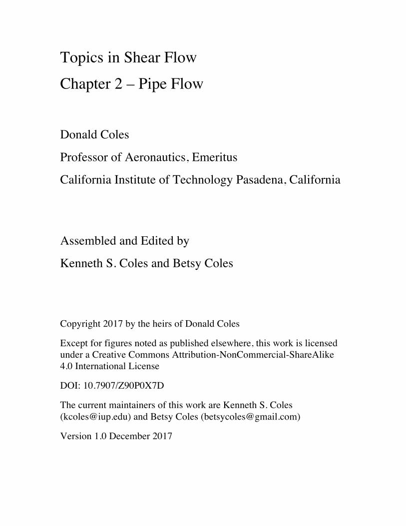
The Reynolds equations of mean motion were derived in SECTION1.3.4 for the cylindrical polar coordinates sketched in FIGURE 2.1.These equations are easily specialized for the case of steady flow ina round pipe of radius R. To make the notation consistent withthat for plane flow, take the axial, radial, and azimuthal coordinatesas (x, r, θ) and the corresponding velocity components as (u, v, w).Take the mean flow to be fully developed, which is to say rectilinear.Thus v = w = 0, and u 6= 0. All derivatives of mean quantitieswith respect to θ are zero, as are all derivatives with respect to xexcept ∂p/∂x, this term being the engine that drives the flow. Thecontinuity equation is moot. For simplicity, the overbar indicatinga mean value will be suppressed hereafter except in the Reynoldsstresses. The three momentum equations are reduced to
0 = −∂p∂x
+1
r
d
drr
(µ
du
dr− ρu′v′
); (2.1)
0 = −∂p∂r
+1
r
(ρw′w′ − d
drr ρv′v′
); (2.2)
2.1. GENERALITIES 61
Figure 2.1: Cylindrical polar coordinate system and
notation for pipe flow.
0 = − 1
r2
d
drr2 ρv′w′ . (2.3)
The fluctuations u′, v′, w′ vanish at the wall. The three equations(2.1)–(2.3) are rigorously correct, and must be satisfied by the meanflow under the specified conditions. The equations are obviously notcomplete, since there are three equations for six unknown quanti-ties. Two of the Reynolds stresses, −ρu′u′ and −ρu′w′, fail to ap-pear. Of these, the absence of the mean product u′w′ is expectedif the turbulent motion is random. Given a sampled value for theaxial fluctuation u′, it is reasonable to suppose, in view of the axialsymmetry of the problem, that positive and negative values for theazimuthal fluctuation w′ are equally probable. That this argumentcan be dangerous will be demonstrated in SECTION 2.5.5, where itleads to a wrong conclusion for the viscous sublayer near a wall. Inthe case of −ρu′u′, the failure of the Reynolds equations even to con-tain this streamwise normal stress is embarrassing. It appears thatnothing can be learned about this stress from the laws of mechanicsin Reynolds-averaged form. At the same time, it is this Reynoldsstress −ρu′u′ that is most easily and most commonly measured.
62 CHAPTER 2. PIPE FLOW
Consider the three equations of motion (2.1)–(2.3). The thirdequation (2.3) has the integral r2ρv′w′ = constant, and the constantis zero whether evaluated on the axis or at the wall. The secondequation (2.2) is more instructive. Formal integration from r to R,with the boundary condition p = pw at the wall, gives
p+ ρv′v′ = pw − ρR∫r
(w′w′ − v′v′
)r
dr . (2.4)
When the lower limit is taken at the pipe axis, r = 0, the integraldiverges unless v′v′ = w′w′ on the axis. The equality is intuitivelyobvious. If two traverses are made along a diameter of the pipeto measure in one case the radial velocity fluctuation v′ along thetraverse direction and in the other case the azimuthal velocity fluc-tuation w′ normal to it, the two measurements must be statisticallyequivalent on the axis.
As the lower limit r in equation (2.4) approaches the upperlimit R, the definite integral is eventually small compared with theterm ρv′v′ on the left. In some vicinity of the wall, therefore, a usefulapproximation suggests itself;
p+ ρv′v′ = pw = constant . (2.5)
This approximation will be examined more closely in SECTION X1.
Finally, the quantity in parentheses in the first momentumequation (2.1) is evidently the total shearing stress τ , here definedwith a change in sign in the derivative and in v′ because y = R − ris a more natural independent variable for an observer viewing theflow from the wall;
τ = −(µ
du
dr− ρu′v′
). (2.6)
At the wall of the pipe, where all velocity fluctuations vanish, thecorresponding value is
τw = −µ(
du
dr
)w
. (2.7)
1Unclear reference, possibly 5.2.1
2.1. GENERALITIES 63
By assumption, the terms in parentheses in equations (2.1) and(2.2) do not depend on x, so that
∂2p
∂x2=
∂2p
∂r∂x= 0 . (2.8)
It follows that ∂p/∂x is a constant, independent of x and r, althoughp itself depends on x and also on r if the flow is turbulent, accordingto equation (2.4). Equation (2.1) in the form
0 = −∂p∂x− 1
r
drτ
dr(2.9)
can therefore be integrated from r to R, with the boundary conditionτ = τw when r = R, to obtain
Rτw − rτ = −(R2 − r2
)2
∂p
∂x. (2.10)
On putting r = 0, this becomes
τw = −D4
∂p
∂x, (2.11)
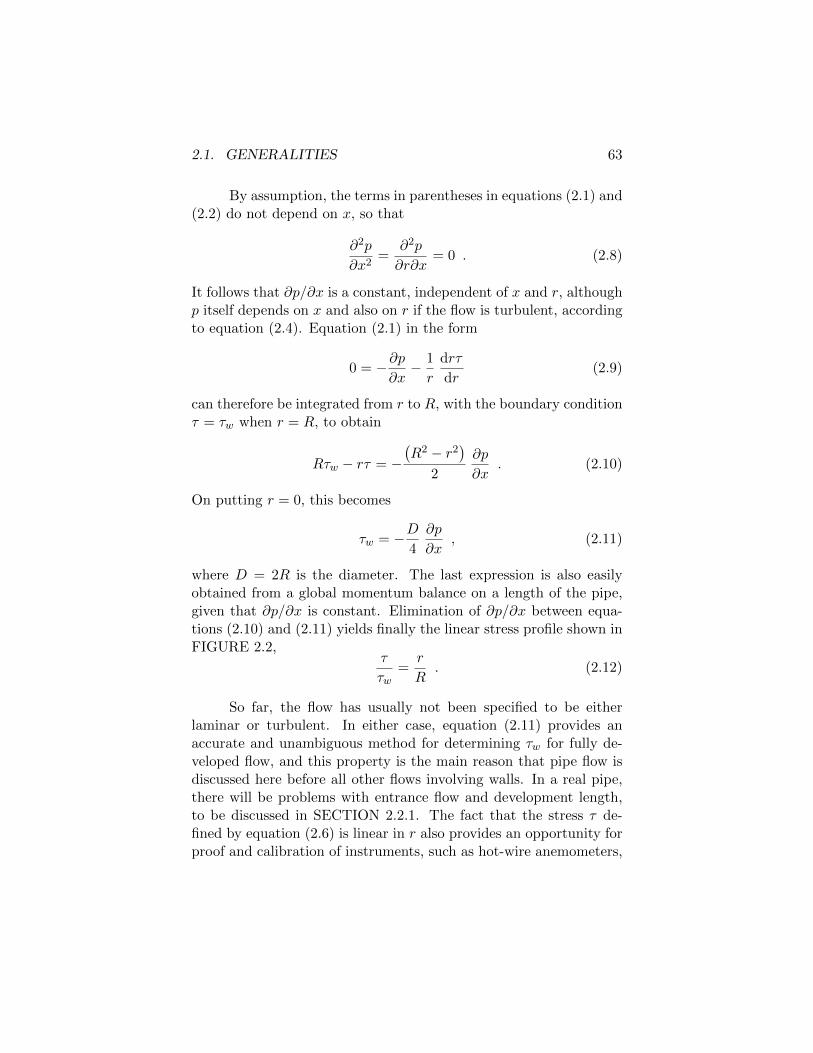
where D = 2R is the diameter. The last expression is also easilyobtained from a global momentum balance on a length of the pipe,given that ∂p/∂x is constant. Elimination of ∂p/∂x between equa-tions (2.10) and (2.11) yields finally the linear stress profile shown inFIGURE 2.2,
τ
τw=
r
R. (2.12)
So far, the flow has usually not been specified to be eitherlaminar or turbulent. In either case, equation (2.11) provides anaccurate and unambiguous method for determining τw for fully de-veloped flow, and this property is the main reason that pipe flow isdiscussed here before all other flows involving walls. In a real pipe,there will be problems with entrance flow and development length,to be discussed in SECTION 2.2.1. The fact that the stress τ de-fined by equation (2.6) is linear in r also provides an opportunity forproof and calibration of instruments, such as hot-wire anemometers,
64 CHAPTER 2. PIPE FLOW
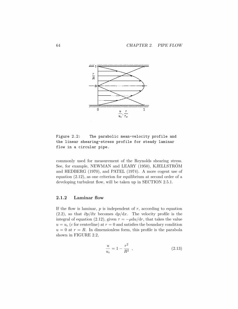
Figure 2.2: The parabolic mean-velocity profile and
the linear shearing-stress profile for steady laminar
flow in a circular pipe.
commonly used for measurement of the Reynolds shearing stress.See, for example, NEWMAN and LEARY (1950), KJELLSTROMand HEDBERG (1970), and PATEL (1974). A more cogent use ofequation (2.12), as one criterion for equilibrium at second order of adeveloping turbulent flow, will be taken up in SECTION 2.5.1.
2.1.2 Laminar flow
If the flow is laminar, p is independent of r, according to equation(2.2), so that ∂p/∂x becomes dp/dx. The velocity profile is theintegral of equation (2.12), given τ = −µdu/dr, that takes the valueu = uc (c for centerline) at r = 0 and satisfies the boundary conditionu = 0 at r = R. In dimensionless form, this profile is the parabolashown in FIGURE 2.2,
u
uc= 1− r2
R2, (2.13)
2.1. GENERALITIES 65
where the centerline velocity uc is related to the other parameters ofthe problem by
τw = 2µucR
. (2.14)
This solution (2.13) of the Navier-Stokes equations for laminar pipeflow, like solutions of the Stokes approximation for low Reynoldsnumbers, represents a balance between pressure forces and viscousforces. However, the transport terms vanish here because of thespecial geometry, not because the Reynolds number is necessarilysmall.
Finally, the volume flow Q in the pipe can be calculated, anda mean velocity u defined, from
Q =
R∫0
2πrudr = πR2u (2.15)
(the tilde, here and elsewhere, is intended as a mnemonic for anintegral mean value). Given equation (2.13) for u, it follows on inte-gration that
u =uc2
. (2.16)
Several of the earliest experiments with pipe flow and withflow between concentric rotating cylinders in the 19th century wereundertaken primarily for a reason that may now seem almost unnat-ural. The equations of NAVIER (1823) and STOKES (1849) inde-pendently incorporate a hypothesis first proposed by NEWTON inhis Principia Mathematica, published in 1687. According to STAN-TON and PANNELL (1914), the proper attribution to Newton wasfirst pointed out by Sir George Greenhill, who would presumablyhave been at home in both the subject and the Latin language. Therelevant passage introduces Section IX, “The circular motion of flu-ids,” in Book II, “The motion of bodies.” In the elegant prose of therevised translation by Cajori (1934):
Hypothesis: The resistance arising from the want of lu-bricity in the parts of a fluid is, other things being equal,
66 CHAPTER 2. PIPE FLOW
proportional to the velocity with which the parts of thefluid are separated from one another.
This hypothesis is explicit in the tensor relation τ = µ def ~uin the introduction. The scalar constant of proportionality, the vis-cosity, is assumed to be an intrinsic or state property of the fluid (itmay, for example, vary significantly with temperature), independentof the motion. In the case of pipe flow, the technique was and isused to show the existence of such a fluid property by showing thatthe quantity µ, expressed theoretically for the case of fully developedlaminar pipe flow by a combination of equations (2.11), (2.14), and(2.16),
µ = − D2
32u
dp
dx, (2.17)
is experimentally independent of particular choices for D and u, sincethese must be precisely compensated for by variations in dp/dx. Asa practical matter, it is usually not the mean velocity u that is mea-sured, but the volume flux Q defined by equation (2.15). Equation(2.17) is therefore better expressed as
µ = − πD4
128Q
dp
dx(2.18)
to emphasize that in capillary-tube viscometry the diameter D needsto be very accurately known. Many common fluids, including air andwater, possess the property of viscosity in the sense just defined andare therefore referred to as Newtonian fluids. A second important is-sue, the validity of the no-slip boundary condition at the wall, has forpractical purposes been resolved experimentally in favor of no slip.Residual doubts about this condition for the case of non-wettingcombinations, such as mercury on glass, or water on tetrafluoroethy-lene (teflon), have been mostly quieted by BINGHAM and THOMP-SON (1928) and by BROCKMAN (1956), respectively. Exceptionsto Newtonian behavior are known, and these present formidable dif-ficulties in formulating a constitutive relationship between the stressand rate-of-strain tensors. The relatively unstructured literature ofrheology and of turbulence modeling testifies, in a familiar idiom,that Newton is a hard act to follow.
2.1. GENERALITIES 67
The Reynolds number for both laminar and turbulent pipe flowis commonly defined in terms of the mean velocity u and the pipediameter D;
Re =uD
ν. (2.19)
Usage varies in defining a dimensionless friction coefficient (seeSECTION X).2 In mechanical and aeronautical engineering, wherethe boundary layer and its global momentum balance are in the fore-ground, the usual form for the dimensionless friction, and the onethat I will adopt here, is
Cf =τw
ρu 2/2. (2.20)
This quantity is also denoted by f and called the Fanning factorby mechanical engineers. For laminar flow, equations (2.14), (2.16),(2.19), and (2.20) imply
Cf =16
Re. (2.21)
To the extent that pipe flow can be viewed as a boundary layeron the inside of a cylindrical body, it might be more consistent touse uc and R instead of u and D in the definition (2.19) for theReynolds number, and u2
c instead of u 2 in the definition (2.20) forthe friction coefficient. Probably the usage described here has sur-vived because no value for uc is available for most of the existingpipe data. In practice, the definition of dimensionless coefficients tocharacterize pipe flow over a large range of Reynolds numbers hasbeen preempted by the turbulent case, for which the wall friction isonly weakly dependent on the viscosity, and the dynamic pressure isthe important reference quantity.
In principle, both τw and u are easily measured for fully de-veloped pipe flow, the former in terms of ∂p/∂x and the latter by avariety of methods. These include direct evaluation from the integraldefinition (2.15), if a velocity profile is available; or measurement ofvolume flow rate, by weighing or by use of a calibrated volume if
2Possibly section 2.4.1
68 CHAPTER 2. PIPE FLOW
the fluid is a liquid; or by blowdown techniques if the fluid is a gas.Other methods include use of a calibrated venturi, orifice plate, orother type of flow meter; or, for best regulation, use of a constant-displacement pump or even a piston-cylinder displacement mecha-nism.
2.1.3 An extremum principle
It was pointed out by LIN (1952), in a short paper whose rootslie in work by HELMHOLTZ (1868) and KORTEWEG (1883) onarbitrarily slow steady viscous motions, that the parabolic laminarprofile in a round pipe can be obtained from an extremum principle.Consider all possible axisymmetric rectilinear motions u(r) satisfyingthe no-slip condition at the wall, and minimize the total rate ofenergy dissipation,
Φ = µ
R∫0
2πr
(du
dr
)2
dr , (2.22)
subject to the constraint of a constant volume flux,
Q =
R∫0
2πrudr = πR2u = constant . (2.23)
The notation Φ means a volume integral of the local rate of dissi-pation over the pipe cross section and over unit length in the flowdirection.
The problem just formulated is an example of what COURANTand HILBERT (1953, Vol. 1, Chapter IV) call the simplest problemin the variational calculus. This is to find the function u(r) thatminimizes the integral
Φ =
R∫0
F (r, u, u′)dr , (2.24)

2.1. GENERALITIES 69
subject to the constraint
Q =
R∫0
G(r, u, u′)dr = constant . (2.25)
The prime here indicates differentiation with respect to r. The Eulerequation for the problem is(
u′′∂2
∂u′∂u′+ u′
∂2
∂u∂u′+
∂2
∂r∂u′− ∂
∂u
)(F + λG) = 0 , (2.26)
where λ is a Lagrange multiplier. In the present case, with
F = 2πµr(u′)2, G = 2πru , (2.27)
equation (2.26) becomes
2µd
dr
(r
du
dr
)− λr = 0 . (2.28)
The indefinite integral of this equation is
u =1
2µ
(λr2
4+A ln r +B
), (2.29)
where A and B are constants of integration. A logarithmic termappears in equation (2.29), but not in equation (2.13), because theearlier derivation already required τ (i.e., du/dr) to be linear in r.The logarithmic term is needed if the no-slip boundary condition isto be satisfied for the more general case of axial flow in an annulus.For flow in a pipe, the boundary conditions u = uc at r = 0 andu = 0 at r = R require A = 0 and B = 2µuc = −λR2/4. Equation(2.14) is recovered,
u
uc= 1− r2
R2, (2.30)
with now
λ = −8µucR2
. (2.31)
70 CHAPTER 2. PIPE FLOW
Use of the three equations (2.31), (2.14), and (2.11) implies
λ = 2dp
dx, (2.32)
as does a direct comparison of equation (2.28) with the laminar ver-sion of the momentum equation (2.1).
For the parabolic profile in a pipe, therefore, the rate of dissi-pation is an extremum. That the extremum is a minimum is easilyshown by adding to the parabolic profile an arbitrary axisymmetricperturbation that vanishes at the wall and does not contribute tothe volume flux. The result (2.32), derived here for a very specialmotion of an incompressible viscous fluid, should be read in the samesitting as SOMMERFELD’s argument (1950, pp. 89–92) that for anincompressible inviscid fluid the pressure p can be interpreted as aLagrange multiplier representing the constraint of incompressibility.
Finally, the pressure gradient and the rate of dissipation canbe related directly for fully developed pipe flow, whether laminar orturbulent. The general form for energy loss from the mean flow perunit time and per unit volume is (cite introduction) τ · grad ~u, sothat equation (2.22) can be written
Φ =
R∫0
2πrτdu
drdr . (2.33)
Integration by parts, with τ = 0 at r = 0 and u = 0 at r = R, gives
Φ = −2π
R∫0
udrτ
drdr . (2.34)
Use of equation (2.12) for τ , (2.15) for the volume flow Q, and (2.11)for τw then gives
Φ = −Q ∂p
∂x. (2.35)
The point of this exercise in the calculus of variations for lam-inar pipe flow is that a similar principle may hold for turbulent flow.If so, it would not be surprising if the resulting mean velocity profileturned out to be logarithmic.
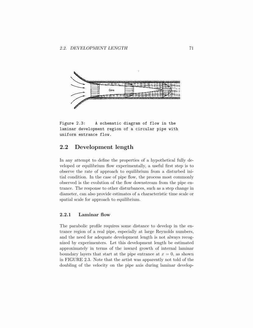
2.2. DEVELOPMENT LENGTH 71
Figure 2.3: A schematic diagram of flow in the
laminar development region of a circular pipe with
uniform entrance flow.
2.2 Development length
In any attempt to define the properties of a hypothetical fully de-veloped or equilibrium flow experimentally, a useful first step is toobserve the rate of approach to equilibrium from a disturbed ini-tial condition. In the case of pipe flow, the process most commonlyobserved is the evolution of the flow downstream from the pipe en-trance. The response to other disturbances, such as a step change indiameter, can also provide estimates of a characteristic time scale orspatial scale for approach to equilibrium.
2.2.1 Laminar flow
The parabolic profile requires some distance to develop in the en-trance region of a real pipe, especially at large Reynolds numbers,and the need for adequate development length is not always recog-nized by experimenters. Let this development length be estimatedapproximately in terms of the inward growth of internal laminarboundary layers that start at the pipe entrance at x = 0, as shownin FIGURE 2.3. Note that the artist was apparently not told of thedoubling of the velocity on the pipe axis during laminar develop-
72 CHAPTER 2. PIPE FLOW
ment. Global parameters available for making the estimate dimen-sionless are the kinematic viscosity ν, the pipe diameter D, and themean velocity u. That the latter quantity is independent of x in thedevelopment region can be shown by reinstating the axisymmetriccontinuity equation in the form
∂u
∂x+
1
r
∂rv
∂r= 0 (2.36)
and calculating the derivative of u from the definition (2.15); thus
πR2 du
dx=
R∫0
2πr∂u
∂xdr = −
R∫0
2π∂rv
∂rdr = 0 , (2.37)
since v vanishes at both limits.
A qualitative estimate of development length in terms of dif-fusion time and transport time can be obtained by using the deviceof a moving observer applied to a growing internal boundary layer.Assume that the entrance is cut square with the axis so that theorigin for x is well defined. Take the flow to be uniform at the pipeentrance; i.e., u = u at x = 0. Vorticity generated at the wall bythe axial pressure gradient diffuses inward through a distance δ in atime t ∼ δ2/ν (see the Rayleigh problem in the introduction).An observer following the mean flow travels a distance x in a timet = x/u. At equal times, x/δ ∼ uδ/ν. If the development length Xis defined as the value of x when δ = D/2, then X is proportional toDRe and x/X is proportional to x/DRe.
Since the first papers by BOUSSINESQ (1890a,b,c; 1891a,b),work on the problem of laminar flow development in a round pipehas become almost a cottage industry. Of more than forty exper-imental, analytical, or numerical papers on this topic, about halfaim at estimates of a particular constant m belonging to the artof capillary-tube viscometry (see the next SECTION 2.2.2). Theremainder view the problem as an exercise in classical fluid mechan-ics. The first analysis using boundary-layer theory was carried outby SCHILLER (1922). This paper was a natural application of theintegral method of Karman and Pohlhausen, published a year ear-lier. The model combined parabolic profiles near the wall with a
2.2. DEVELOPMENT LENGTH 73
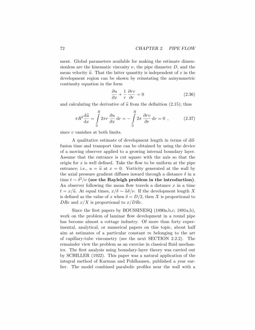
X/(R&)D
FIGURE 3.25. SOme analytical results for laminar flow development in a smooth pipe. The dependent variable uc/u has an asymptotic limit of 2
. -
Figure 2.4: Some analytical results for laminar flow
development in a smooth pipe. The dependent variable
uc/u has an asymptotic limit of 2.
flat profile near the centerline. The predicted evolution of the axialvelocity on the pipe axis is one of the curves shown in FIGURE 2.4.The analysis ignores the fact that a boundary-layer approach is com-plicated by effects of lateral curvature and by interaction betweenthe axial pressure gradient in the inviscid core flow and the grow-ing displacement thickness of the boundary layer, each affecting theother. Moreover, the boundary-layer approximation fails before theflow development is complete, and an asymptotic analysis is even-tually required. The growing power of computers now allows thelaminar problem to be treated by numerical integration of the fullNavier-Stokes equations for quite large Reynolds numbers.
The other data in FIGURE 2.4 are chosen from the work of
DORSEY (1926)MULLER (1936) figure 4ATKINSON and GOLDSTEIN (1938)LANGHAAR (1942) figure 1ASTHANA (1951)TATSUMI (1952)SIEGEL (1953)

74 CHAPTER 2. PIPE FLOW
RIVAS and SHAPIRO (1956)BOGUE (1959)TOMITA (1961)CAMPBELL and SLATTERY (1963)COLLINS and SCHOWALTER (1963)LUNDGREN et al. (1964)SPARROW et al. (1964) figure 3CHRISTIANSEN and LEMMON (1965) figures 2, 3HORNBECK (1965) figures 3, 6McCOMAS and ECKERT (1965)VRENTAS et al. (1966) figures 3–8McCOMAS (1967)FRIEDMANN et al. (1968) figures 1–4LEW and FUNG (1968) tablesSCHMIDT and ZELDIN (1969)FARGIE and MARTIN (1971) figure 4CHEN (1973) figure 1KESTIN et al. (1973) figure 8KANDA and OSHIMA (1986) figures 5–8
The main imperfection of these contributions lies in the fre-quent assumption of a flat velocity profile at the station x = 0, withan unphysical upstream flow that is often left undefined. However,there is general agreement that the independent variable x/DRe isa natural and appropriate one in the laminar development region,whether a boundary-layer model is used or not.
A few experiments include the work of
BOND (1921)RIEMAN (1928)ZUCROW (1929)KLINE and SHAPIRO (1953)SHAPIRO et al. (1954)KREITH and EISENSTADT (1957)WELTMANN and KELLER (1957)RESHOTKO (1958) figure 9PFENNINGER (1961) figure 12

2.2. DEVELOPMENT LENGTH 75
McCOMAS and ECKERT (1965) figure 3ATKINSON et al. (1967) figure 4DAVIS and FOX (1967) figure 11EMORY and CHEN (1968)BERMAN and SANTOS (1969) figures 3–7BURKE and BERMAN (1969) figures 3–6, 8FARGIE and MARTIN (1971) figure 4WYGNANSKI and CHAMPAGNE (1973)MESETH (1974)MOHANTY and ASTHANA (1979)
(Why does nobody plot τw? Mention honeycombs. No calcula-tions for square-cut entrance with bubble.)
From all of this work, the evidence is persuasive that develop-ment is complete for practical purposes when
1
Re
x
D≈ 0.07 ≈ 1
14, (2.38)
provided that the Reynolds number Re is not less than about 100.For a pipe of given diameter and length, the largest Reynolds numberfor which a parabolic profile can be established is about 14L/D. Fora given Reynolds number, the smallest L/D is about Re/14. Con-sequently, to identify the record holder for highest Reynolds numberwith fully developed laminar flow, it is necessary only to look forlarge values of L/D and to test the state of the exit flow. By thiscriterion, the record is about uD/ν = 13,000 and is held by LEITE(1958).
With sufficient care, it is possible to maintain laminar flowin relatively short pipes up to very large Reynolds numbers, 50,000or more. However, the parabolic profile is never fully developed insuch cases, and the decisive element for transition becomes the dis-turbance level outside the boundary layer in the early developmentregion. In any contest to establish the highest achievable laminarReynolds number in short pipes, the results are a measure of the de-gree of care taken to avoid such disturbances, rather than of any di-rectly useful physical quantity. For example, blowdown methods canreduce disturbance levels far below the best obtainable in flows driven
76 CHAPTER 2. PIPE FLOW
by an upstream pump or compressor, and a gas flow can be quietedby use of a sonic orifice to isolate the test section from a downstreampump. As far as I know, the record here is held by PFENNINGERand MEYER (1953), who used a long conical contraction fitted with13 screens, as well as elaborate vibration isolation, to obtain a flowfree of turbulence at a Reynolds number uD/ν = 88,000. The corre-sponding number ux/ν was about 50 × 106, an order of magnitudehigher than the number that can be obtained on flat plates in con-ventional wind tunnels. The boundary layer in Pfenninger’s pipeoccupied about 60 percent of the area at the pipe exit. To obtain afully developed parabolic profile in air under these conditions wouldneed a length of about 140 meters, together with heroic measuresto minimize disturbances in the flow and to account for changes indensity. Even if this could be done, I see no particular profit froman attempt.
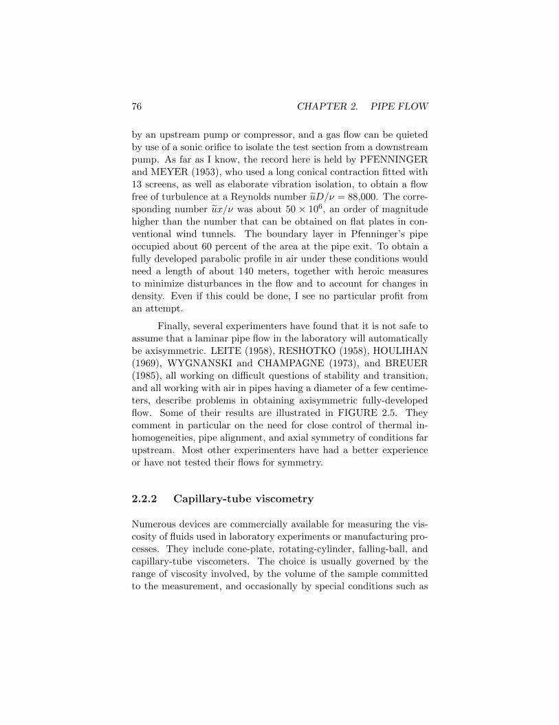
Finally, several experimenters have found that it is not safe toassume that a laminar pipe flow in the laboratory will automaticallybe axisymmetric. LEITE (1958), RESHOTKO (1958), HOULIHAN(1969), WYGNANSKI and CHAMPAGNE (1973), and BREUER(1985), all working on difficult questions of stability and transition,and all working with air in pipes having a diameter of a few centime-ters, describe problems in obtaining axisymmetric fully-developedflow. Some of their results are illustrated in FIGURE 2.5. Theycomment in particular on the need for close control of thermal in-homogeneities, pipe alignment, and axial symmetry of conditions farupstream. Most other experimenters have had a better experienceor have not tested their flows for symmetry.
2.2.2 Capillary-tube viscometry
Numerous devices are commercially available for measuring the vis-cosity of fluids used in laboratory experiments or manufacturing pro-cesses. They include cone-plate, rotating-cylinder, falling-ball, andcapillary-tube viscometers. The choice is usually governed by therange of viscosity involved, by the volume of the sample committedto the measurement, and occasionally by special conditions such as
2.2. DEVELOPMENT LENGTH 77
Figure 2.5: Several examples from the experimental
literature showing non-axisymmetric laminar flow in
circular pipes. The most likely cause is secondary flow
due to thermal inhomogeneity in a gravitational field or
asymmetry of the upstream channel.
78 CHAPTER 2. PIPE FLOW
a need in process work to immerse the device in the bulk fluid. Typ-ically, such viscometers are calibrated by the manufacturer or theuser, using fluids of known viscosity, to take into account variouseffects of finite geometry.
The question of how a known viscosity comes to be known isfar from trivial. This question is the business of standards labora-tories. For example, SWINDELLS, COE, and GODFREY (1952)describe a painstaking program in capillary-tube viscometry, carriedon from 1931 to 1941 and from 1947 to 1952 at the U.S. NationalBureau of Standards (now the U.S. National Institute of Standardsand Technology), whose singular result was to establish the valueµ = 0.010019± 0.000003 poise for pure water at 20 ◦C. This value isstill the cornerstone of viscosity tables for water that are constructedfrom more extensive but less accurate measurements. The geometryin capillary viscometry at the standards level is apparently stan-dardized, requiring a square-cut entrance and exit, although othergeometric details, such as the tube outer diameter, are usually leftopen. The need for close control of several variables is self-evident. Inorder to obtain four significant figures in the viscosity, according toequation (2.18), the absolute temperature, the volume flow rate, thetube length, the pressure difference, and especially the tube diametermust all be known to better accuracy, with a further allowance forerrors introduced by differentiation of experimental data. It may benecessary, for example, to represent the cross section of a real tubeby an ellipse rather than by a circle, with a corresponding adjust-ment in the theory. A long tube of small diameter provides an easilymeasurable pressure difference, although this pressure difference isnecessarily global rather than local if pressure taps cannot be pro-vided along the length of the tube. At the same time, the diametermust not be so small that it cannot be measured with the necessaryaccuracy. The length is also limited in practice by the need to main-tain the flow system at constant temperature in a bath of practicalsize without having to coil the tube and accept a much more complextheory.
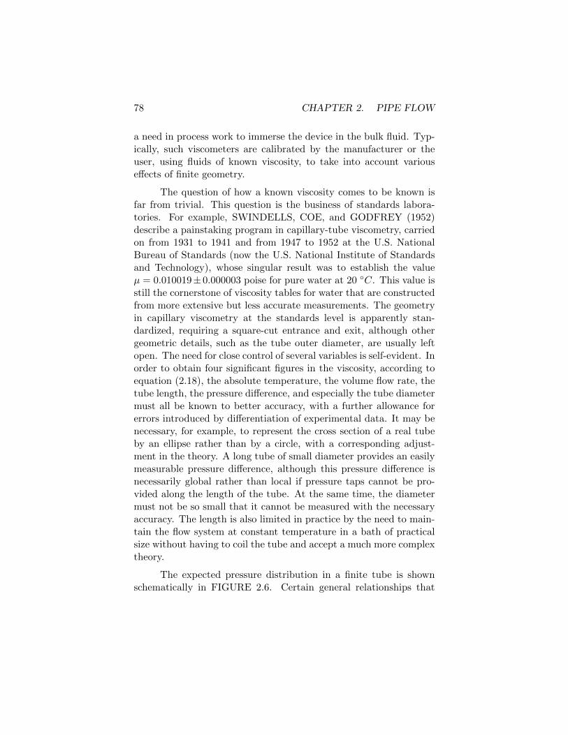
The expected pressure distribution in a finite tube is shownschematically in FIGURE 2.6. Certain general relationships that
2.2. DEVELOPMENT LENGTH 79
Figure 2.6: A schematic representation of the
pressure distribution along a tube of length L with
uniform entrance flow at x = 0. The flow may be laminar
or turbulent and the cross section need not be circular.
emerge from the figure do not depend on the shape of the tube crosssection or the shape of the tube entrance, as long as these are fixed.Suppose for convenience that entrance and exit are cut square, sothat L is well defined. The quantities p0 and p2 are the static pres-sures in the entrance and exit reservoirs. The quantity p′1 is thestatic entrance pressure associated with a fictitious fully developedflow over the full length of the tube. Anomalous pressure effects atboth entrance and exit are included in principle, although exit effectsare not treated explicitly. It is not necessary to distinguish betweenlaminar and turbulent flow, or even mixed flow at Reynolds numbersin the transition regime.
The strategy associated with FIGURE 2.6 is one of experi-mental differentiation. Suppose that the Reynolds number is heldconstant as the length of the tube is varied, and suppose that theshortest tube is long enough to achieve fully developed flow. Thena unit increment in the length of the tube will give rise to a unit
80 CHAPTER 2. PIPE FLOW
increment in total pressure drop. Begin with the identity
p0 − p2 = (p0 − p′1) + (p′1 − p2) . (2.39)
For the general case, define an ideal friction coefficient for fully de-veloped flow,
Cf =D (p′1 − p2)
2Lρu 2, (2.40)
where u = Q/A is again a mean velocity over the cross section A.For the special case of a circular tube, the definition (2.40) reducesthrough equation (2.11) to equation (2.20). Define also a globalfriction coefficient,
Cf =D (p0 − p2)
2Lρu 2, (2.41)
where the circumflex over Cf denotes a mean value over the entirelength of the tube, reservoir to reservoir. Equation (2.39) then takesthe form
CfL
D=
(p0 − p′1)
2ρu 2+ Cf
L
D. (2.42)
For fully developed flow at the exit, the first term on the right is aconstant that is characteristic of the complete development processfor particular entrance conditions and Reynolds number. Withoutthe factor of 2 in the denominator, this constant is usually denotedby m in the literature of capillary-tube viscometry;
m =(p0 − p′1)
ρu 2, (2.43)
so that
CfL
D=m
2+ Cf
L
D. (2.44)
Except possibly for a square-cut entrance, the development parame-ter m, defined graphically in figure 2.6, will depend on the entrancegeometry and flow conditions for a particular tube. A plot of CfL/Dagainst L/D is a straight line whose slope Cf and intercept m/2 arecharacteristic for the Reynolds number in question. In particular,
Cf =∂ (Cf L/D)
∂ (L/D). (2.45)
2.2. DEVELOPMENT LENGTH 81
A simple implementation of this differentiation scheme wasproposed and used by COUETTE (1890), but has since been usedonly rarely, and then mostly by professionals such as Swindells et al .The technique is to construct two capillary viscometers by connect-ing two tubes in series with a third reservoir inserted between them.The two tubes are assumed to be identical in diameter and all othergeometrical details except length. When in equilibrium, they havethe same flow rate. The two parameters Cf and m are then readilyevaluated from a single experiment.
Discuss m from p(x). Cite bibliography.
Equation (2.44) is usually cast in a more direct and more literalform for use in viscometry with a round tube. From equation (2.39),with p′1 − p2 = −Ldp/dx = 4Lτw/D = 8µuL/R2, and with u =Q/πR2, this form is
π2R4 (p0 − p2)
ρQ2= m+
8πµL
ρQ. (2.46)
For constant Q and R and variable L, a dimensional plot of (p0−p2)against L yields a straight line whose slope is proportional to µ andwhose intercept is proportional to m. Such a plot is a practicalrealization of FIGURE 2.6.
A different form, appropriate for a single tube with changingflow rate, is obtained on multiplying by Q and making the importantassumption that m is independent of Reynolds number;
π2R4 (p0 − p2)
ρQ= mQ+
8πµL
ρ. (2.47)
Now, for constant L and R and variable Q, a plot of (p0 − p2)/Qagainst Q yields a straight line whose slope is proportional to m andwhose intercept is proportional to µ. This formulation is the one usedby Swindells et al. Such a plot is sometimes called a Knibbs plot,after KNIBBS (1895). The assumption that the entrance parameterm defined by equation (2.44) is independent of Reynolds number insome range of Re needs verification for both smooth and square-cutentrances, since the parameters u, D, and ν define two lengths, Dand ν/u, together with their ratio Re.

82 CHAPTER 2. PIPE FLOW
Finally, still for a single tube, multiplication of equation (2.47)by ρQ yields
π2R4 (p0 − p2) = ρmQ2 + 8πµLQ . (2.48)
The conclusion that the overall pressure drop should be the sum ofa term in Q (or u) and a term in Q2 (or u2) was noted by HAGEN(but not by Poiseuille) and is probably the reason that the termcontaining m is often referred to, not quite correctly, as a kinetic-energy correction.
For the case of a circular tube, it is also possible to calculatep0 − p′1 in FIGURE 2.6 from first principles, given a suitable modelof the flow in the development region. By definition,
m =(p0 − p′1)
ρu 2=
(p0 − p1) + (p1 − p2)− (p′1 − p2)
ρu 2. (2.49)
Visualize an ideal entrance, for which the velocity profile at an initialstation x = 0 is uniform, with velocity u and pressure p1 that do notdepend on r. Assume frictionless acceleration from rest upstream ofthis station. The Bernoulli equation then determines the first termon the right in equation (2.49);
p0 − p1 =1
2ρu 2 . (2.50)
The middle term can be partially evaluated for laminar flow.For steady axisymmetric laminar flow in the development region,the equations of motion (see introduction) can be written, withno boundary-layer approximation, as
∂ru
∂x+∂rv
∂r= 0 ; (2.51)
ρ
(∂ruu
∂x+∂ruv
∂r
)= −r ∂p
∂x+ µr
(∂2u
∂x2+
1
r
∂
∂rr∂u
∂r
). (2.52)
When both equations are integrated over a cross section of a tube ofconstant diameter, the result can be reduced to a simple momentum
2.2. DEVELOPMENT LENGTH 83
integral,
d
dx
R∫0
(ρuu+ p)rdr +Rτd = 0 , (2.53)
where τd, the local viscous stress at the wall, is a function of x in thedevelopment region (d for development).
Now integrate equation (2.53) from x = 0 to x = L. At x = 0the flow is uniform, with velocity u and pressure p1. At x = L, theflow is fully developed. The static pressure p2 is then independent ofr, according to the laminar version of equation (2.2). The velocityprofile u(r) at x = L is the parabolic distribution (2.13), with ucreplaced by 2u. Integration of equation (2.53) gives
p1 − p2 =1
3ρu 2 +
2
R
L∫0
τd dx . (2.54)
Finally, consider a fictitious fully developed flow over the length L,for which
p′1 − p2 = −L dp
dx= 2
L
Rτw =
2
R
L∫0
τw dx . (2.55)
Substitution of equations (2.50), (2.54), and (2.55) in (2.49) yields
m =1
2+
1
3+
2
R
L∫0
(τd − τw)
ρu 2dx . (2.56)
This formula is not commonly quoted. I have encountered it only inthe textbook by WHITE (1974, p. 336).
The numerous calculations mentioned in the previous SEC-TION 2.2.1 almost invariably assume that the flow is uniform at theentrance station x = 0, so that equation (2.56) qualifies as a properdefinition for m. All that is then required from the calculation is thequantity τd in the development region, although most authors havechosen to report instead the pressure at the wall or the velocity on
84 CHAPTER 2. PIPE FLOW
the axis. In equation (2.56), flow adjustment near the tube exit hasbeen ignored. There is evidence (where; cite refs) that this ap-proximation is valid for Reynolds numbers greater than about 100,on the empirical ground that a jet from a sharp-edged orifice intoa large reservoir of the same fluid comes to rest without significantpressure recovery (ref). Some commercial capillary-tube viscome-ters have a flared or rounded exit, and the exit pressure recoverymay be finite and sensitive to Reynolds number.
An experimenter might not concede that direct calculation ofm from equation (2.56) or some equivalent equation is either neces-sary or desirable. For a given entrance geometry, fluid, and flow rate,m is a well-defined number. However, it is not necessarily the samenumber for a tube with a square-cut entrance, common in viscom-etry at the standards level, as for a tube with a rounded entrance,common in some commercial capillary-tube viscometers. The modelleading to equation (2.56) makes no distinction. It assumes that thewall friction τd begins abruptly at x = 0 with an integrable singu-larity. For a smooth entrance it is likely, and for a sharp entrance itis certain, that the boundary layer is not being described correctly.In effect, the pressure p1 and the length L are legislated rather thandefined unambiguously by the geometry. Mention Hagenbach,Wilberforce, Boussinesq, Swindells, Schiller on m.
Mickelson. There remains the empirical differentiation schemeof equation (2.45), which does not involve p1. Some nice measure-ments reported in the thesis by MICKELSON (1964) were designedto exploit the simple empirical approach represented by this equa-tion. Mickelson worked at a more than ordinary level of accuracy,although not at the level of a standards laboratory. He measuredthe total pressure drop between reservoirs for water flowing in tenglass tubes having the same nominal diameter of 0.1 cm but differentvalues of L/D ranging from 15 to 510. The tubes had a square-cutentrance and exit, so that L is well defined. The volume flow wasregulated by a positive-displacement gear pump whose noise leveland speed regulation are not described in detail. Most of the mea-surements described here were made at 30 ◦C, and I have takenthe viscosity of water at this temperature to be 0.007975 poise (ref)
2.2. DEVELOPMENT LENGTH 85
3}
10-2
10-3 '------'----''---'---'--'-...L.L..L-'------''--L-...I.--I-I.............'-'--_''--....................................
1cP 103 lOA 105
Re
Figure 2.7: The raw friction data of MICKELSON (1964)
for ten capillary tubes of fixed diameter and various
lengths ranging from L/D = 15 to L/D = 510. The
fluid is water at 30 ◦C. The curve for turbulent flow
at the right is faired through Nikuradse’s data. Note
that transition is slightly delayed for the two longest
tubes.
rather than the value 0.008007 used by Mickelson. The calculationsthat follow mostly reproduce Mickelson’s work, and my results arein very good agreement with his.
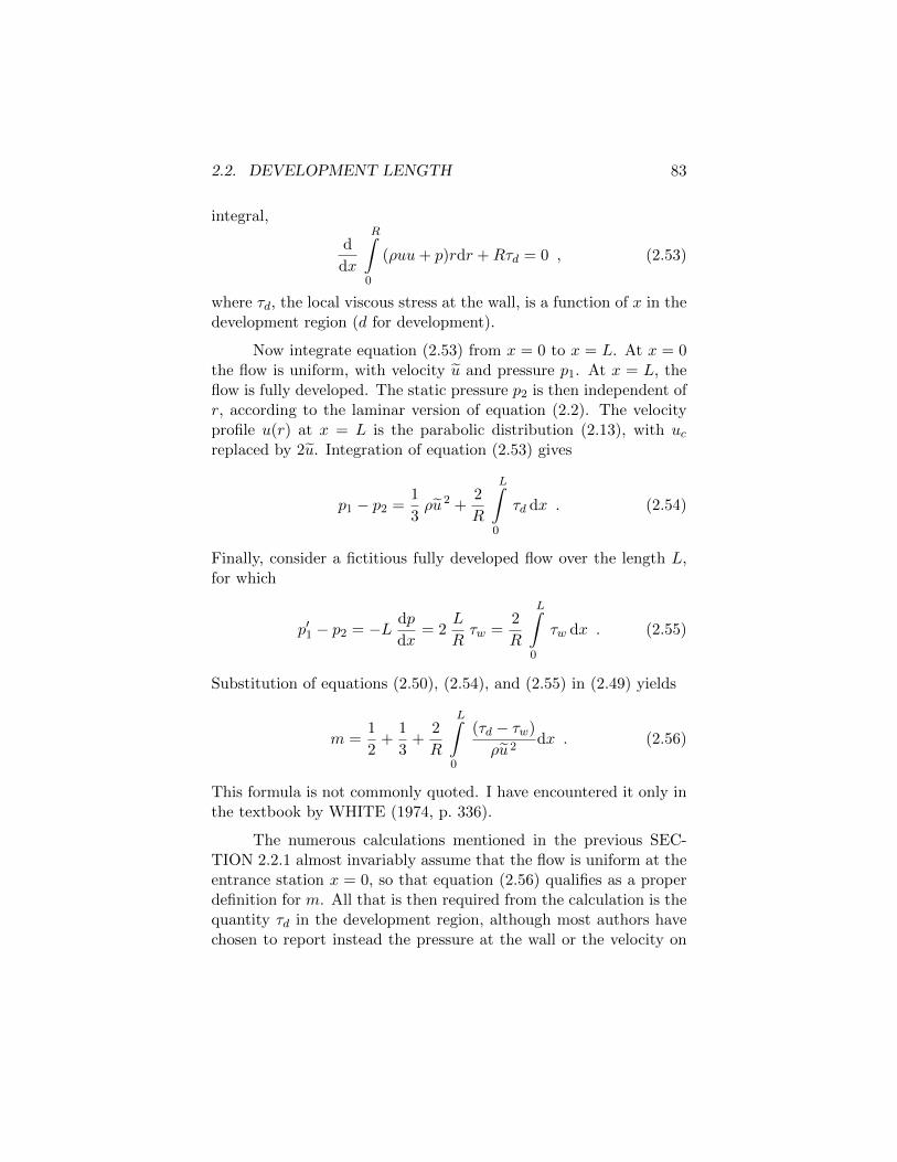
Mickelson tabulated the global pressure difference CfL/D, which
he called fm. His raw data for Cf as a function of Re, with L/Das parameter, are shown in FIGURE 2.7. Because Mickelson wasinterested in turbulent flow as a prototype problem for viscometricstudies of complex rheological fluids, he included measurements forturbulent flow of water. These measurements will be discussed in thenext SECTION 2.2.3.
The differentiation of experimental data according to equation
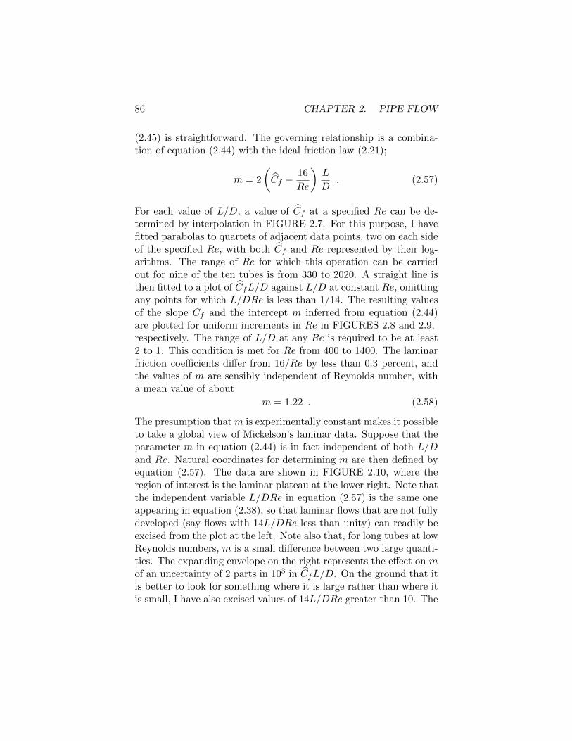
86 CHAPTER 2. PIPE FLOW
(2.45) is straightforward. The governing relationship is a combina-tion of equation (2.44) with the ideal friction law (2.21);
m = 2
(Cf −
16
Re
)L
D. (2.57)
For each value of L/D, a value of Cf at a specified Re can be de-termined by interpolation in FIGURE 2.7. For this purpose, I havefitted parabolas to quartets of adjacent data points, two on each sideof the specified Re, with both Cf and Re represented by their log-arithms. The range of Re for which this operation can be carriedout for nine of the ten tubes is from 330 to 2020. A straight line isthen fitted to a plot of CfL/D against L/D at constant Re, omittingany points for which L/DRe is less than 1/14. The resulting valuesof the slope Cf and the intercept m inferred from equation (2.44)are plotted for uniform increments in Re in FIGURES 2.8 and 2.9,respectively. The range of L/D at any Re is required to be at least2 to 1. This condition is met for Re from 400 to 1400. The laminarfriction coefficients differ from 16/Re by less than 0.3 percent, andthe values of m are sensibly independent of Reynolds number, witha mean value of about
m = 1.22 . (2.58)
The presumption that m is experimentally constant makes it possibleto take a global view of Mickelson’s laminar data. Suppose that theparameter m in equation (2.44) is in fact independent of both L/Dand Re. Natural coordinates for determining m are then defined byequation (2.57). The data are shown in FIGURE 2.10, where theregion of interest is the laminar plateau at the lower right. Note thatthe independent variable L/DRe in equation (2.57) is the same oneappearing in equation (2.38), so that laminar flows that are not fullydeveloped (say flows with 14L/DRe less than unity) can readily beexcised from the plot at the left. Note also that, for long tubes at lowReynolds numbers, m is a small difference between two large quanti-ties. The expanding envelope on the right represents the effect on mof an uncertainty of 2 parts in 103 in CfL/D. On the ground that itis better to look for something where it is large rather than where itis small, I have also excised values of 14L/DRe greater than 10. The
2.2. DEVELOPMENT LENGTH 87
10-2
10-3 L...-----l_.L-1.-L...Jc...LLLL-_-'---....l...-.L....L...L...Lw..L_--'---'--'-.L..J....JL...L.J..J
1~ 1~ 1~ 1~ Re
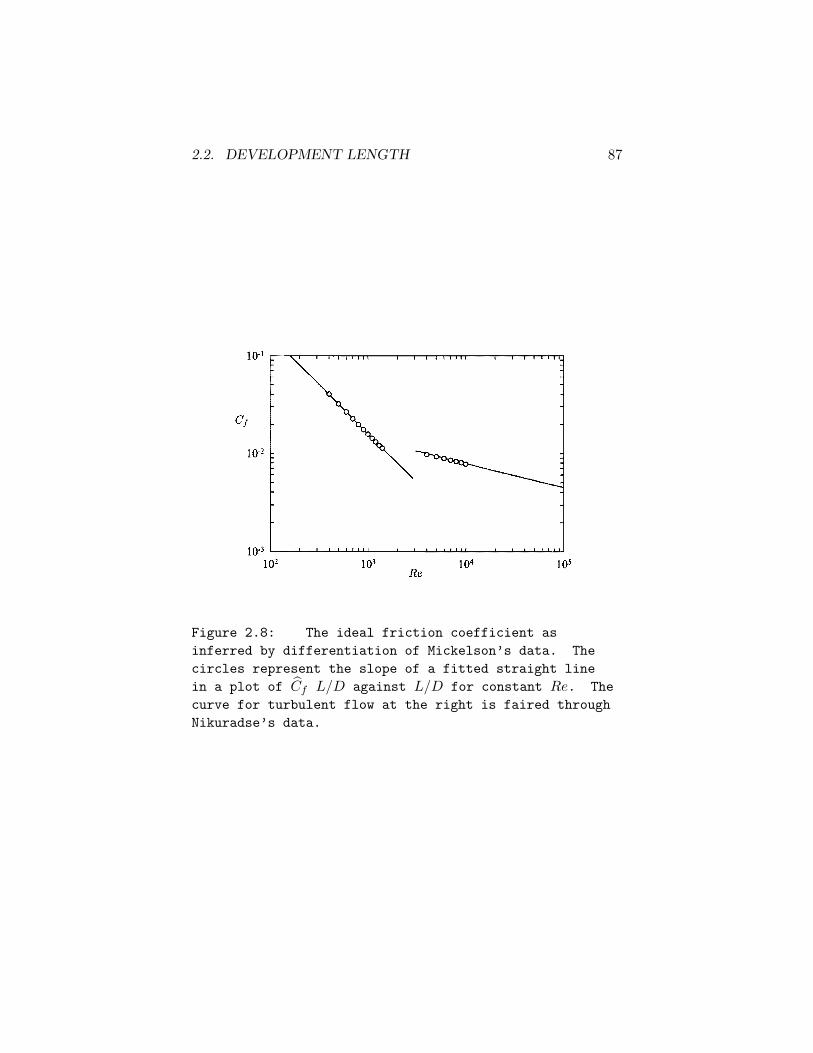
Figure 2.8: The ideal friction coefficient as
inferred by differentiation of Mickelson’s data. The
circles represent the slope of a fitted straight line
in a plot of Cf L/D against L/D for constant Re. The
curve for turbulent flow at the right is faired through
Nikuradse’s data.

88 CHAPTER 2. PIPE FLOW
0.80
o~~~~~~U-__~~~~~__~~~~~
l~ 1~ 1~ 1~ Re
Figure 2.9: The laminar flow-development parameter mas a function of Re for a square-cut entrance according
to Mickelson’s data. The open circles show twice the
intercept of a fitted straight line in a plot of Cf L/Dagainst L/D for constant Re. In the laminar range, the
small filled circles are from equation (2.57).
2.2. DEVELOPMENT LENGTH 89
~. j
2 (OJ _~) L Re D
16 L
ReD
•
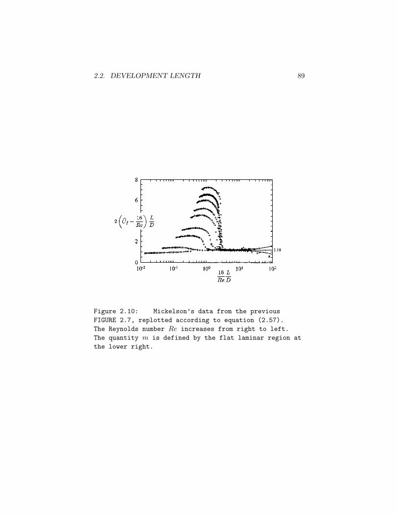
Figure 2.10: Mickelson’s data from the previous
FIGURE 2.7, replotted according to equation (2.57).
The Reynolds number Re increases from right to left.
The quantity m is defined by the flat laminar region at
the lower right.
90 CHAPTER 2. PIPE FLOW
surviving data are plotted as small solid circles in FIGURE 2.9. Inprinciple, a single observation would suffice to determine m by thismethod. In practice, the mean of 110 values is
m = 1.19 , (2.59)
with a dispersion of a few percent. There is no clear indication ofany dependence of m on Reynolds number.
One anomaly in these experiments was pointed out by Mickel-son and is visible in FIGURE 2.7. The tubes of intermediate lengthshow essentially normal behavior in the transition regime, which liesas expected in the range 2000 < Re < 2800 (see SECTION 2.3.1).The two longest tubes do not. The reason is unknown.
The data in FIGURE 2.10 are consistent with the previousestimate for the minimum length required to achieve a fully devel-oped laminar flow in a pipe with a square-cut entrance; namely,L/D = Re/14. At this condition the penalty paid for entry lossesamounts to about a third of the overall pressure drop. This topic isdeveloped further in SECTION X3, where the subject is the use ofhoneycombs for flow control and for measurement of flow rate.
This discussion of Mickelson’s work is out of chronological or-der, but is presented first because I consider this work to be the bestavailable evidence for the value of the laminar (or turbulent) param-eter m. Theory must yield to experiment, at least for the case of asquare-cut entrance. In this context, two important papers from the19th century are more typical in showing the early evolution of theconcept of viscosity and capillary viscometry.
Poiseuille. A paper on pipe flow of water by POISEUILLE(1846) belongs on any short list of fundamental contributions to theart of experimental fluid mechanics. This work was first reportedin three short notes in Comptes Rendus (1840a, 1840b, 1841). Thenovelty and importance of the research caused the French academyto appoint a committee to verify the methods and results and judgetheir suitability for publication in full. The favorable report of thiscommittee was published twice in French and once in German (see
3Reference unclear, possibly a section that was not completed.

2.2. DEVELOPMENT LENGTH 91
ARAGO et al. 1842, 1843a, 1843b), and Poiseuille’s full paper fol-lowed in due course in Memoires Presentes par Divers Savants. Aftera lapse of almost a century, the latter paper was translated into En-glish at the instance of a distinguished rheologist, E.C. Bingham,who added some critical notes. The tabulated data had earlier beenreprinted by BINGHAM as Appendix D of his monograph Fluidityand Plasticity (1922), and some typographical errors in this appendixwere later corrected by BINGHAM (1930).
A short account of Poiseuille’s life and work, with emphasis onthe paper of 1846, can be found in a recent appreciation by SUTERAand SKALAK (1993). Poiseuille was a physician interested in theflow of blood, especially in vessels of capillary dimension. He at-tempted some measurements in vivo, but concluded that controlledexperiments would be required to formulate the laws governing bloodflow, and turned to experiments with water in glass tubing of verysmall inside diameter, as small as 14µm.
Poiseuille attacked the problem with an admirable combina-tion of skill and luck. Knowing nothing of the concept of streamlineflow, he was comfortable with a square-cut entrance. Consequently,the length of his tubes, except for the shortest ones, was well de-fined. Moreover, the method of construction of his glass apparatusrequired him to decrease the length of his tubes by removing succes-sive downstream portions, leaving the entrance geometry unchanged.An experimenter today might well adopt the same strategy by design.
Poiseuille determined systematically that the flow rate in manyof his tubes was directly proportional to the pressure drop and tothe fourth power of the diameter, and inversely proportional to thelength; thus
Q = K ′′hD4
L. (2.60)
The units of Q in equation (2.60) are mm3/ sec. The overall pressuredrop h (called P by Poiseuille) is in mm Hg, and L and D are in mm.The units of K ′′ are then (sec ·mm Hg)−1. For a fixed temperatureof 10 ◦C, Poiseuille reported the average value of the dimensional
92 CHAPTER 2. PIPE FLOW
constant K ′′ for a variety of experiments as
K ′′ = 2495.224 , (2.61)
in which the first four digits may be significant. When the lengthsin Q, h, L, and D are all expressed in cm, and the pressure dropis written as 4p = ρmgh, where ρm is the density of the manome-ter fluid and g is the acceleration of gravity, Poiseuille’s empiricalequation (2.60) becomes (clear up signs)
Q = 10K ′′D4
ρmg
4pL
. (2.62)
Comparison with the theoretical equation (2.18) derived in SEC-TION 2.1.2,
Q =πD4
128µ
dp
dx, (2.63)
shows that Poiseuille was dealing with the combination
K ′′ =πρmg
1280µ, (2.64)
under the implicit assumption that entrance effects were negligible;i.e., that ∆p/L could be identified with dp/dx. The values quoted byPoiseuille for g and ρm are g = 980.8 cm/sec2 at the latitude of Parisand ρm = 13.57 gm/cm3 for mercury at a manometer temperatureof 11.5 ◦C. Consequently, his numerical result (2.61) is equivalent to
µ = 0.01309gm
cm sec. (2.65)
The unit used for this quantity in the CGS system has come tobe called the poise, following a suggestion by DEELEY and PARR(1913). The accepted value today for water at 10 ◦C is 0.01307 poise.Poiseuille also obtained data for viscosity at other temperatures be-tween 0 ◦C and 45 ◦C, with errors never larger than one percent.
Poiseuille was intuitively aware of the entrance effect, althoughhe had no way to define it quantitatively. The main sequence of hisexperiments consists of 34 tables for six tubes of different diameters,each of which was progressively shortened as the work proceeded. He
2.2. DEVELOPMENT LENGTH 93
separated these results into a first series, for which the pressure dropwas found to be very nearly inversely proportional to flow time fora fixed flow volume, as in equation (2.60), and a second series thatshowed a more complex behavior. The two series are plotted sepa-rately in the two upper curves in FIGURE 2.11. Poiseuille did notattempt to explain the difference in behavior, although he did notethat most of the data of the second series were associated with shorttubes at high flow rates. A brief inspection of the tables confirmsthat development of the parabolic profile in these tubes probably didin fact occupy a large fraction, up to and exceeding the whole, of thetube length.
Recall the entrance parameter m defined by equation (2.57)above, for which a numerical value m = 1.19 (assumed to be inde-pendent of Reynolds number) was extracted from Mickelson’s datain FIGURE 2.9 of SECTION 2.2.2. For a square-cut entrance,
m = 2
(Cf −
16
Re
)L
D, (2.66)
where Cf is an empirical friction coefficient that distributes the totalpressure drop uniformly over the length of the pipe. The ideal frictioncoefficient Cf has been replaced by 16/Re. Rearrangement of thisequation gives
Cf Re = 16 + 8m
(Re
16
D
L
). (2.67)
This form applies as long as the quantity in parenthesis is less thanunity; i.e., as long as the parabolic profile is established somewherewithin the pipe.4 One is use of the precise theoretical laminar fric-tion law, Cf Re = 16. The other is use of the approximate empiricalcondition L/ReD ≥ 0.06, which I take as L/ReD ≥ 1/14, for theparabolic profile to be fully developed. With this proviso, the cor-
4A sentence at this point in the 1997 draft read, ”Note that the number 16 ap-pears in these formulas, by deliberate coincidence, in two different ways.” Authorevidently removed the sentence after recalculating equation 2.38 in Section 2.2.1and revising the approximate value from 1/16 (0.06) to 1/14 (0.07). He revisedthe result where he employed it in the discussion after equation (2.57), but nothere. We leave it to the reader to revise what follows.

94 CHAPTER 2. PIPE FLOW
101
10-3
10-1 102
Re
Figure 2.11: A modern representation of POISEUILLE’s
data (1846) for flow in capillary tubes. Note the
displaced scales. The first series is suitable for
determining the viscosity. The second series in
uncorrected form is not. The lowest display shows the
second series after a correction for flow development.
The residual scatter here may be caused by inaccurate
measurement of tube length.
2.2. DEVELOPMENT LENGTH 95
rection (2.44) for entrance effect is accurate as long as
Cf Re ≤ 16 + 8m . (2.68)
For m = 1.19, this isCf Re ≤ 25.5 . (2.69)
The equality in this equation defines the dotted line near the middlecurve in FIGURE 2.11. Below this line, the original data of thesecond series are shown by open circles; above the line, by filledcircles. The ideal or corrected value of the friction coefficient forfixed L/D is obtained by subtracting a constant from Cf ;
Cf = Cf −m
2
D
L. (2.70)
When this correction with m = 1.19 is applied to all of the dataof the middle curve in FIGURE 2.11, the result is as shown in thebottom curve. The symbols are the same.
Poiseuille’s data show no obvious effect of transition, and leaveopen the question of the possible dependence of m on Re. Each of histables for the first series and the (corrected) second series generates aline with the proper slope of −1 in logarithmic coordinates, but witha constant that varies more or less randomly from the ideal value of16 for the product Cf Re, sometimes by several percent or more. Thisobservation implies that one of the two fixed parameters for such aline (L, D) must have been incorrectly measured. My candidate is L,mostly because the problem worsens in the second series, where L issmall. The extreme case is a run with very small and uncertain lengthand moderate Reynolds numbers, a run that another author mighthave discarded. My comments are consistent with the conclusionby several authors that Poiseuille’s data are not sharp enough todetermine m accurately, although they are sharp enough to benefitfrom a correction. At the other extreme of accuracy, the evidenceshows that Poiseuille succeeded in measuring the diameter of histubes to an accuracy comparable to the wave length of visible light.He refers to the instrument he used as a camera lucida. After findinga description of this device in an old encyclopedia, I understand whythe French committee was impressed.
96 CHAPTER 2. PIPE FLOW
I have a mild reservation about the lack of scatter in the tablein Poiseuille’s section 130. The seven numbers listed for K ′′ are eachtraceable to a single measurement, whose flow volume was recalcu-lated to correspond to standard values for pressure drop (775 mm Hg),tube length (25 mm), and flow duration (500 sec). The adjustmentwas carried out in terms of proportionalities, which Poiseuille re-ferred to as laws. Constants of proportionality did not appear, andno statistical measures were used except in the final average for K ′′.A different choice for the selected single measurements out of thedozens available would almost certainly increase the scatter in K ′′.
This criticism aside, I think that the skill and insight demon-strated by Poiseuille transcend his exaggerations as to accuracy. Theexecution and interpretation of the measurements are remarkable,considering the state of the fluid-mechanical art at the time. In 1840there was no precedent for expecting or requiring integer exponentsin what amounts to a dimensional statement. In fact, there was noprecedent for dimensional statements. Even a name for the hypo-thetical fluid property at issue, the viscosity, was lacking. Moreover,Poiseuille worked completely outside the small establishment dedi-cated to the activity that we now call basic research.
Finally, one remark is needed about priority for the empiricalequation (2.62) and the theoretical equation (2.63). In the litera-ture, the theoretical equation is sometimes erroneously attributedto Poiseuille. In fact, this integral of the equations of motion waspublished some years later by at least six authors, (check Hagen),
WIEDEMANN (1856) JACOBSON (1860)HAGENBACH (1860) STEFAN (1862)HELMHOLTZ (1860) MATHIEU (1863)
among whom Jacobson attributes the result to unpublished notesby Neumann. Together, these writers probably hold the record fornumber of authors arriving independently and almost simultaneouslyat a single theoretical result.
Both NAVIER (1823) and STOKES (1849) in their originalpapers considered pipe flow as a problem suitable for applicationof the new equations of motion for a viscous fluid. Navier’s result
2.2. DEVELOPMENT LENGTH 97
contained a wrong exponent, with Q varying like D3 rather than likeD4. This discrepancy was noted by Poiseuille, who did not attemptto revise Navier’s analysis. Stokes derived the parabolic profile, butdid not calculate the flow rate because at the time he had reservationsabout the no-slip condition. If he had known of Poiseuille’s work,published in final form three years earlier, these reservations surelywould never have arisen.
(DISCUSS HAGEN 1839, 1854)
Need paragraphs on pipe flow of air with something aboutMillikan oil-drop experiment, Maxwell’s result.
As L/D → 0, a tube with square-cut entrance and exit be-comes an orifice, and it can be expected that the flow will becomeindependent of L/D provided that the reservoirs are very large, withflat walls and thin boundary layers near the orifice (not pipe flow).Data in the transition region for L/D were published by Kreith andEisenstadt. These data are very ragged, and I think that the orificediameters were not under good control. The data for their test rigs1, 2, 3, nominally identical, differ by 30 percent. The quantity calledCfL/D becomes a pressure coefficient Cp.
For other data see
BOND (1921)ZUCROW (1929)LINDEN and OTHMER (1949)KLINE and SHAPIRO (1953)SHAPIRO et al. (1954)IVERSON (1956)CAMPBELL and SLATTERY (1963)MICKELSON (1964)EMORY and CHEN (1968)LEW and FUNG (1968)BENDER (1969)FARGIE and MARTIN (1971)MOHANTY and ASTHANA (1979)
As the tube becomes shorter, the first observable effect is that
98 CHAPTER 2. PIPE FLOW
the parabolic profile is not achieved, and the pressure gradient is ev-erywhere larger than the fully developed value. For short enoughtubes, the reattachment region becomes involved with the exit flow.(This is not a practical problem, except that it prevents getting thebubble length from the pressure drop.) Finally, reattachment doesnot occur at all, and the flow shows a vena contracta, unless Re isof order unity or less. (Include drag of perforated plate?)
2.2.3 Turbulent flow
Mickelson also observed turbulent flow in his tubes, as already shownin FIGURE 2.7. The empirical differentiation scheme leading toequation (2.45) is equally useful for the case of developed turbulentflow, although the ideal friction law is not known a priori . Mickel-son’s data for turbulent flow are included in FIGURE 2.9 and FIG-URE 2.8 for 4000 < Re < 10000. The value of m appears to beclose to 0.80 for a square-cut entrance. (Check other sources;see Bingham p 18.) The accuracy imputed to Mickelson’s datafor laminar flow is a fraction of one percent. If the same accuracycan be imputed to the data for turbulent flow, and I believe thatit can, in spite of the small diameters involved, these measurementscan be taken as definitive for fully developed turbulent pipe flow inthe specified Reynolds-number range.
Estimates of required development length for turbulent pipeflow play an important part in the design of test facilities in whichthe flow is intended to achieve classical turbulent equilibrium. If in-termittent turbulence is to be avoided (see SECTION 2.3.1), theReynolds numbers of interest are larger than about 3000. FIG-URES 2.12 and 2.13 show, in terms of evolution of centerline velocity,two modes of development. On the one hand, in FIGURE 2.12 theentrance flow is moderately quiet, and laminar boundary layers de-velop in the normal way. However, disturbances, although small,are large enough to cause transition in the boundary layer, whichthen grows rapidly because of enhanced mixing. The centerline ve-locity can decrease locally near transition because the displacementthickness decreases while the momentum thickness continues to in-

2.2. DEVELOPMENT LENGTH 99
Figure 2.12: Typical experimental results for
turbulent flow development in a smooth pipe when
transition occurs in the boundary layer well downstream,
near the peak in the curve of uc against x. The
turbulent asymptotic limit for uc/u depends on Reynolds
number and is here approached from above.

100 CHAPTER 2. PIPE FLOW
Figure 2.13: Typical experimental results for
turbulent flow development in a smooth pipe when
transition occurs in the boundary layer very close to
the entry. The turbulent asymptotic limit for uc/udepends on Reynolds number and is approached from below.

2.2. DEVELOPMENT LENGTH 101
crease. On the other hand, in FIGURE 2.13 the entrance flow isdeliberately made noisy, by one means or another. The boundarylayer becomes turbulent quickly, and the centerline velocity then ap-proaches an equilibrium value from below, as in laminar flow. AtRe = 100, 000, for example, the boundary layer can be turbulent onediameter from the entrance. In either figure, the equilibrium value ofuc/u depends on Reynolds number, according to experience reviewedin SECTION X.5
Studies of turbulent flow development include
BROOKS et al. (1943)DEISSLER (1950)BARNES (1952)BRENKERT (1954)BARBIN and JONES (1963)WILLIAMS (1969)RICHMAN and AZAD (1973)SHARAN (1974)WANG and TULLIS (1974)WEIR et al. (1974)REICHERT and AZAD (1976)UEMURA and IMAICHI (1977, 3G)LAWS et al. (1979)KLEIN (1981)
Variables on the axis include uc and u′u′. Variables at thewall include Cf and p.
Finally, there is the obvious advantage of a square-cut entranceas a standard tripping device. The flow near a square-cut entrancewill be marked by a separation bubble and by Kelvin-Helmholz insta-bility of the associated inflected profile. (Cite Schiller.) Radial pres-sure gradients near the reattachment point may mean for very shortpipes that flow adjustment near the exit should not be neglected.
For data, see
5Unclear reference, possibly a section not completed.
102 CHAPTER 2. PIPE FLOW
SCHILLER (1922)KIRSTEN (1927)DEISSLER (1950)BARBIN and JONES (1963)BRIGHTON (1965)SHARAN (1972)WANG and TULLIS (1974)POZZORINI (1976)REICHERT and AZAD (1976)HANKS et al. (1979)LAWS et al. (1979)KLEIN (1981)
Protocol for estimating required development length for turbu-lent pipe flow. Produce two log-log plots of x/D against Re, one eachfor quiet and noisy entrance flow. Use different symbols for flows thatpass or fail.
(1) If τ is linear in r, flow passes. See Kjellstrom and Hedberg,Brighton, Bourke et al, Barbin and Jones, Patel, Sharan, Wygnanskiand Champagne, Wichner, Gessner, Bremhorst and Walker, Chenand Robertson, Brookshire, Powe and Townes, Schildknecht et al.
(2) If uc/u is normal, flow passes. See Weir et al, Reichert andAzad, Deissler, Wang and Tullis, Laws et al, Brenkert. For normalvalues, see Rotta, Senecal and Rothfus, Patel and Head, Morrow,Clark, Nikuradse, and all profile data.
(3) If u′/u on centerline is normal, flow passes. See Pennellet al and all data on Reynolds stresses.
(4) If uc/uτ is normal, flow passes. Similar to (2), but requiresCf to be normal also. See discussion in section on friction coefficientand value of Karman’s κ.

2.3. TRANSITION 103
2.3 Transition
2.3.1 Intermittency
All classical flows pass through a transition from laminar to tur-bulent flow as the Reynolds number increases. However, transitionprocesses, like similarity rules, are very different from one classicalflow to another. In most cases, nature does not provide a continuumof flow states that evolve gradually from a recognizably laminar flowat one transition boundary to a recognizably turbulent flow at theother. It is more common to find autonomous regions of laminarand turbulent flow that are separated by irregular but well definedinterfaces. The local state of such flows at any point in space andtime is usually described by a binary number γ(t), called the inter-mittency, that takes the values γ = 0 if the flow is laminar and γ = 1if the flow is turbulent. Methods for classifying the state as laminaror turbulent will be taken up in the next section. The mean value γ,usually averaged over time or ensemble, will be called the intermit-tency factor. For the purposes of this monograph, the intermittencyfactor can be interpreted as the fraction of time that the flow at afixed point spends in the turbulent state.
There is ample experimental, analytical, and numerical evi-dence that fully developed laminar pipe flow is unconditionally sta-ble for Reynolds numbers Re = uD/ν below about 2000. No matterhow disturbed the initial state of the flow may be, the state fardownstream relaxes to the laminar parabolic profile. For Reynoldsnumbers above about 2800, an initial disturbed state leads eventuallyto continuous turbulence that is usually assumed to be homogeneousin the flow direction, although this assumption may not have beensufficiently tested. In an intermediate range of Reynolds numbers,2000 < Re < 2800, transition far downstream from a noisy entrancetakes the form of alternating regions of laminar and turbulent fluidmoving down the pipe.
Experimental observations of intermittency in pipe flow beganvery early. REYNOLDS (1883), using a dye filament for flow visual-ization, described intermittent dispersion of the dye filament by rapid
104 CHAPTER 2. PIPE FLOW
local mixing. HAGEN (1854) and COUETTE (1890) independentlynoted large fluctuations in the trajectory of a water jet emerginghorizontally from a square-cut pipe exit into air. These fluctuationsoccurred only for a small range of flow rates and were accompaniedby changes in the appearance of the jet surface (“glassy,” “frosty”).The explanation is easier today than it was a century ago. Underthe action of gravity, the trajectory of the exit jet in free fall froma horizontal pipe is very nearly a parabola. For a fixed volume flux,the momentum flux is greater by a factor 4/3 when the exit velocityprofile is parabolic than when the exit velocity profile is uniform (asan approximation to a turbulent exit profile). The experiment is bestcarried out with a long pipe of small enough diameter so that surfacetension forces are relatively large, although not large enough to causeearly breakup of the jet. Otherwise, slow fluid near the outside of theinitial free jet may fall away before it can be accelerated by internalviscous forces. This latter phenomenon is visible in some scenes inthe educational motion picture by STEWART (1969).
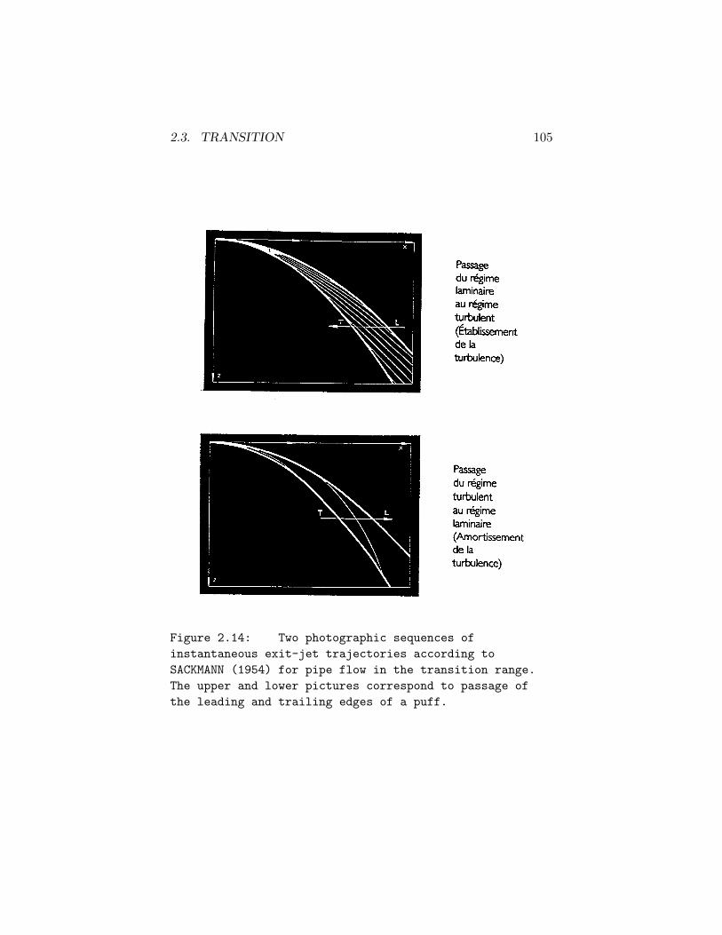
After an interval during which the range of Reynolds numbersfor transition was well established by measurements of mean flowrate and mean pressure drop, the behavior of the exit jet in transi-tion was revisited by SACKMANN (1947–1954) in a series of shortpapers in Comptes Rendus. These papers have little structure or con-tent beyond the content of FIGURE 2.14, which is taken from thepaper of 1954. I believe that the images are analytical versions of jettrajectories derived from motion-picture frames for the transitionslaminar → turbulent and turbulent → laminar. There is a dramaticdifference between the slow transition at the leading or downstreamedge of a turbulent region and the rapid transition at the trailing orupstream edge.
Two major contributions to the subject of transition in pipeflow were published almost simultaneously by ROTTA (1956) andLINDGREN (1957). Lindgren worked in water; Rotta worked inboth water and air. Both investigators used a highly disturbed entry.Both analyzed recorded analog signals manually to observe the re-laxation of the flow to an intermittent state. Two quantities that arerelatively easily measured by ignoring details of shape are the global
2.3. TRANSITION 105
Figure 2.14: Two photographic sequences of
instantaneous exit-jet trajectories according to
SACKMANN (1954) for pipe flow in the transition range.
The upper and lower pictures correspond to passage of
the leading and trailing edges of a puff.
106 CHAPTER 2. PIPE FLOW
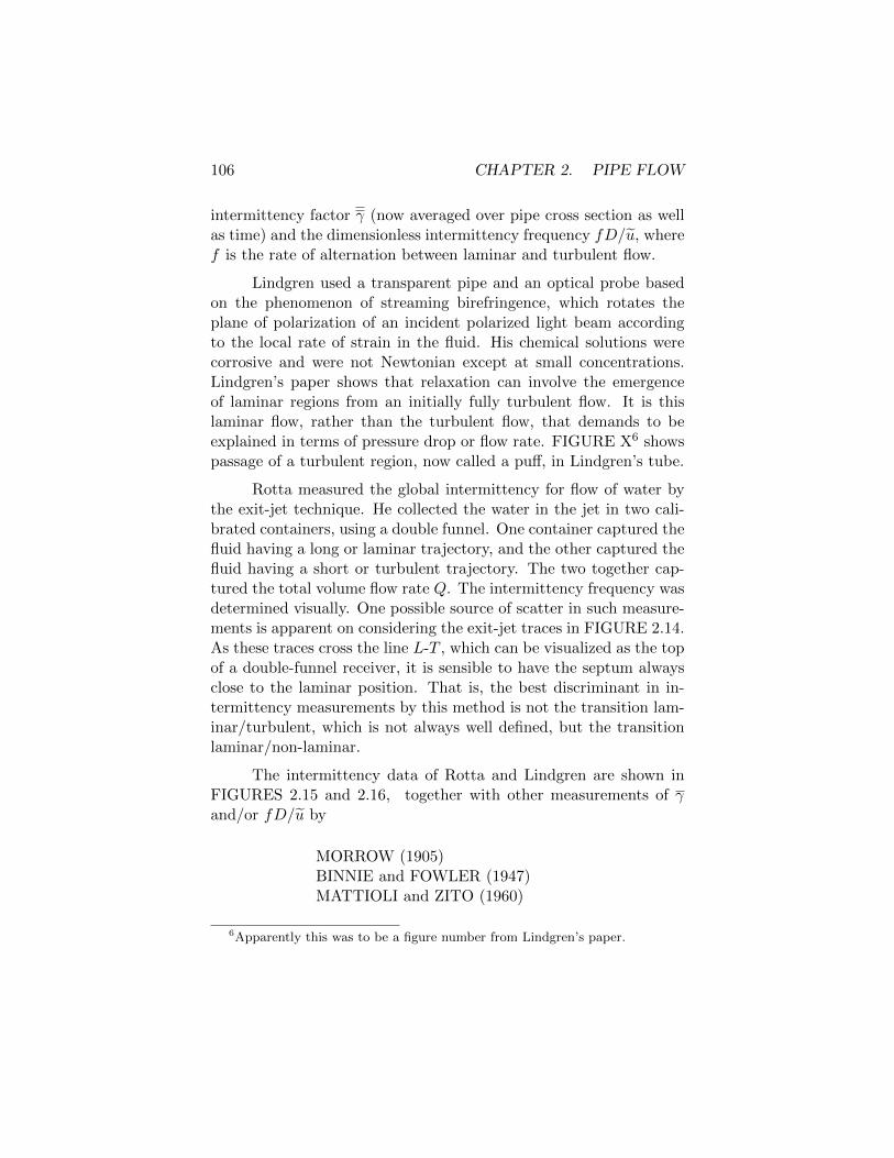
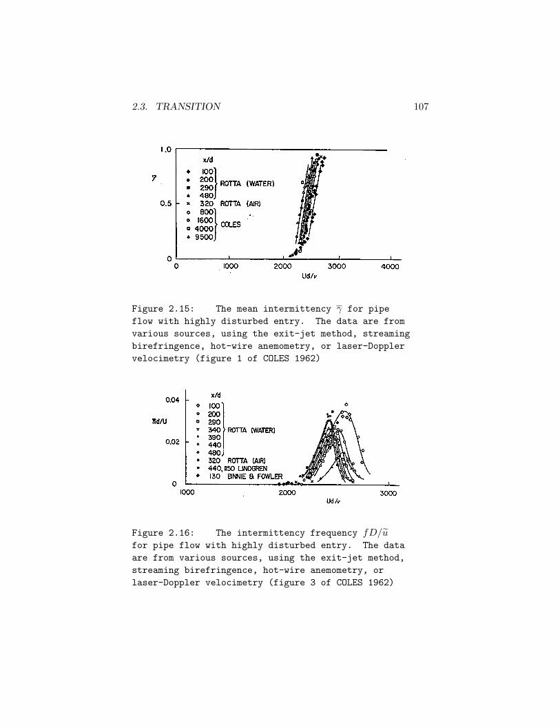
intermittency factor γ (now averaged over pipe cross section as wellas time) and the dimensionless intermittency frequency fD/u, wheref is the rate of alternation between laminar and turbulent flow.
Lindgren used a transparent pipe and an optical probe basedon the phenomenon of streaming birefringence, which rotates theplane of polarization of an incident polarized light beam accordingto the local rate of strain in the fluid. His chemical solutions werecorrosive and were not Newtonian except at small concentrations.Lindgren’s paper shows that relaxation can involve the emergenceof laminar regions from an initially fully turbulent flow. It is thislaminar flow, rather than the turbulent flow, that demands to beexplained in terms of pressure drop or flow rate. FIGURE X6 showspassage of a turbulent region, now called a puff, in Lindgren’s tube.
Rotta measured the global intermittency for flow of water bythe exit-jet technique. He collected the water in the jet in two cali-brated containers, using a double funnel. One container captured thefluid having a long or laminar trajectory, and the other captured thefluid having a short or turbulent trajectory. The two together cap-tured the total volume flow rate Q. The intermittency frequency wasdetermined visually. One possible source of scatter in such measure-ments is apparent on considering the exit-jet traces in FIGURE 2.14.As these traces cross the line L-T , which can be visualized as the topof a double-funnel receiver, it is sensible to have the septum alwaysclose to the laminar position. That is, the best discriminant in in-termittency measurements by this method is not the transition lam-inar/turbulent, which is not always well defined, but the transitionlaminar/non-laminar.
The intermittency data of Rotta and Lindgren are shown inFIGURES 2.15 and 2.16, together with other measurements of γand/or fD/u by
MORROW (1905)BINNIE and FOWLER (1947)MATTIOLI and ZITO (1960)
6Apparently this was to be a figure number from Lindgren’s paper.
2.3. TRANSITION 107
Figure 2.15: The mean intermittency γ for pipe
flow with highly disturbed entry. The data are from
various sources, using the exit-jet method, streaming
birefringence, hot-wire anemometry, or laser-Doppler
velocimetry (figure 1 of COLES 1962)
Figure 2.16: The intermittency frequency fD/ufor pipe flow with highly disturbed entry. The data
are from various sources, using the exit-jet method,
streaming birefringence, hot-wire anemometry, or
laser-Doppler velocimetry (figure 3 of COLES 1962)

108 CHAPTER 2. PIPE FLOW
COLES (1962)VALLERANI (1964)GILBRECH and HALE (1965)YELLIN (1966)CASTRO and SQUIRE (1967)OHARA (1968)PATEL and HEAD (1969)STERN (1970)WYGNANSKI and CHAMPAGNE (1973)CLAMEN and MINTON (1977)RAMAPRIAN and TU (1979)STETTLER and HUSSAIN (1986)
The transition range 2000 < Re < 2800 can be picked out clearly.Some of the scatter in these figures may be traceable to insufficientpipe length or to poor control of temperature. With better control,it is conceivable that such measurements could provide an acceptablemeans for measuring viscosity.
The terms “noisy entrance flow” and “far downstream” mayneed clarification. The work of several investigators (refer to Schil-ler, Prandtl) suggests that flow separation at a square-cut entranceis a sufficient but not excessive disturbance, capable of causing tran-sition in the range of Re just defined. If stronger initial turbulence isdesired, various axisymmetric geometries can be used as variationson the square-cut entry. These include an orifice plate, a step in-crease in diameter, and a bluff central body. All of these geometriesinvolve separated flow and free shear layers that rapidly undergotransition, filling the pipe with turbulence near the entrance if it isnot already full. The first measurements of the distance requiredfor such a noisy flow to relax to an equilibrium intermittent statewere made by Rotta. This distance can be 500 diameters or more,depending on the Reynolds number. It is important, for the sakeof statistical security, to have a large number of alternations withinthe pipe. If the flow rate is independently regulated, then a givenpipe is longest at about Re = 2400. Rotta was not certain about thefinal state of his flows far downstream, and may have supposed thatthis state would always be either fully laminar or fully turbulent.
2.3. TRANSITION 109
To test this point, I once caused some double-funnel measurementsto be made for water in a pipe 9500 diameters long (D = 0.2 cm,L = 1900 cm). The data were obtained by students as a laboratoryproject, and the students were a little careless about temperatureand thus Reynolds number. The original data have been lent andlost. However, the results were reported in a survey paper (COLES1962) and showed γ increasing from 0 to 1 in the standard rangeof Re from 2000 to 2800. The data are included in FIGURE 2.15.For practical purposes, I consider 9500 diameters to be infinity, andI am quite satisfied that the final equilibrium state in the transitionregime is a statistically steady state of intermittent turbulence.
2.3.2 Methods of measurement
The exit-jet phenomenon is peculiar to pipe flow and perhaps tochannel flow. Other experimental techniques for measuring inter-mittency have been developed for other shear flows, and a shortdigression to describe these techniques is in order. (Cite Hedleyand Keffer 1974 and Narasimha 1985.) The classification of aflow as locally laminar or turbulent is always somewhat subjective,but different observers using different signals and different methodstend to obtain similar results. In my experience, the most useful andreliable criterion for classifying a flow as turbulent is the presenceof fluctuations at high frequencies, since such fluctuations will decayand disappear if they are not being continuously supplied with freshenergy through a hypothetical cascade mechanism. This observationexplains why intermittency measurements did not become routineuntil after the development of instruments capable of detecting andrecording turbulent fluctuations.
The property of intermittency near free edges of turbulentshear flows was first noted explicitly by CORRSIN (1943) for thecase of a round jet, although it has always been an obvious featureof clouds and of smoke plumes from chimneys and open fires, andalso appears in photographs of projectile wakes going back to thework of MACH (18xx) (check). I have consulted several colleaguesin an effort to determine why the phenomenon of intermittency was
110 CHAPTER 2. PIPE FLOW
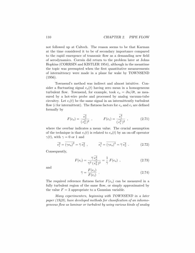
not followed up at Caltech. The reason seems to be that Karmanat the time considered it to be of secondary importance comparedto the rapid emergence of transonic flow as a demanding new fieldof aerodynamics. Corrsin did return to the problem later at JohnsHopkins (CORRSIN and KISTLER 1954), although in the meantimethe topic was preempted when the first quantitative measurementsof intermittency were made in a plane far wake by TOWNSEND(1956).
Townsend’s method was indirect and almost intuitive. Con-sider a fluctuating signal eo(t) having zero mean in a homogeneousturbulent flow. Townsend, for example, took eo = ∂u/∂t, as mea-sured by a hot-wire probe and processed by analog vacuum-tubecircuitry. Let ei(t) be the same signal in an intermittently turbulentflow (i for intermittent). The flatness factors for eo and ei are definedformally by
F (eo) =e4o
( e2o )2
, F (ei) =e4i
( e2i )2
, (2.71)
where the overbar indicates a mean value. The crucial assumptionof the technique is that ei(t) is related to eo(t) by an on-off operatorγ(t), with γ = 0 or 1 and
e2i = (γeo)
2 = γ e2o , e4
i = (γeo)4 = γ e4
o . (2.72)
Consequently,
F (ei) =γ e4
o
γ2 ( e2o )2
=1
γF (eo) , (2.73)
and
γ =F (eo)
F (ei). (2.74)
The required reference flatness factor F (eo) can be measured in afully turbulent region of the same flow, or simply approximated bythe value F = 3 appropriate to a Gaussian variable.
Many experimenters, beginning with TOWNSEND in a laterpaper (1949), have developed methods for classification of an inhomo-geneous flow as laminar or turbulent by using various kinds of analog
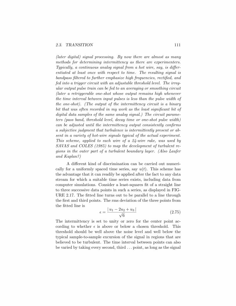
2.3. TRANSITION 111
(later digital) signal processing. By now there are almost as manymethods for determining intermittency as there are experimenters.Typically, a continuous analog signal from a hot wire, say, is differ-entiated at least once with respect to time. The resulting signal isbandpass filtered to further emphasize high frequencies, rectified, andfed into a trigger circuit with an adjustable threshold level. The irreg-ular output pulse train can be fed to an averaging or smoothing circuit(later a retriggerable one-shot whose output remains high wheneverthe time interval between input pulses is less than the pulse width ofthe one-shot). (The output of the intermittency circuit is a binarybit that was often recorded in my work as the least significant bit ofdigital data samples of the same analog signal.) The circuit parame-ters (pass band, threshold level, decay time or one-shot pulse width)can be adjusted until the intermittency output consistently confirmsa subjective judgment that turbulence is intermittently present or ab-sent in a variety of hot-wire signals typical of the actual experiment.This scheme, applied to each wire of a 24-wire rake, was used bySAVAS and COLES (1985) to map the development of turbulent re-gions in the outer part of a turbulent boundary layer. (Also Lauferand Kaplan?)
A different kind of discrimination can be carried out numeri-cally for a uniformly spaced time series, say u(t). This scheme hasthe advantage that it can readily be applied after the fact to any datastream for which a suitable time series exists, including data fromcomputer simulations. Consider a least-squares fit of a straight lineto three successive data points in such a series, as displayed in FIG-URE 2.17. The fitted line turns out to be parallel to a line throughthe first and third points. The rms deviation of the three points fromthe fitted line is
ε =|u1 − 2u2 + u3 |√
6(2.75)
The intermittency is set to unity or zero for the center point ac-cording to whether ε is above or below a chosen threshold. Thisthreshold should be well above the noise level and well below thetypical sample-to-sample excursion of the signal in regions that arebelieved to be turbulent. The time interval between points can alsobe varied by taking every second, third . . . point, as long as the signal

112 CHAPTER 2. PIPE FLOW
Figure 2.17: A least-squares fit to three successive
points of a uniformly spaced time series for a variable
u(t).
contains appreciable turbulent energy. In my experience it has usu-ally been possible to choose the two parameters of the method, thesampling frequency and the threshold level, so that γ is not sensitiveto either. The resulting time series of ones and zeros can be edited asmany times as desired by assigning to each point the value belongingto a majority of points in a group of 3, 5, . . . symmetrically placedpoints.
Several writers since Townsend have proposed as a first ap-proximation an on-off transition model. That is, intermittent pipeflow should be viewed as a quite literal alternation between fully de-veloped laminar and turbulent regimes. By observing the DC andlow-frequency components of a hot-wire signal in a flow of air atR = 2550, ROTTA (1956) found that the axial velocity at a fixedpoint fluctuated between two values characteristic of laminar andturbulent flow respectively. These values are shown in FIGURE 2.18together with the mean profile indicated in the same flow by a heav-ily damped pitot tube. Although neither of the momentary profilesyields the correct mass flow, which was independently measured bymeans of a downstream sonic orifice, the momentary state of the flowseems always to be close to one limiting profile or the other. Support-
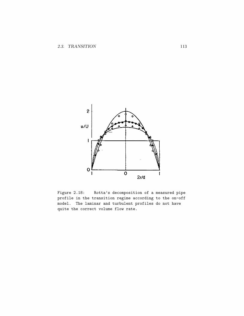
2.3. TRANSITION 113
Figure 2.18: Rotta’s decomposition of a measured pipe
profile in the transition regime according to the on-off
model. The laminar and turbulent profiles do not have
quite the correct volume flow rate.
114 CHAPTER 2. PIPE FLOW
ing evidence for this conclusion can also be drawn from Lindgren’swork. The pressure records in figures 5.9 and 5.10 of his 1957 pa-per allow an estimate of the local axial pressure gradient inside arelatively long turbulent plug. At both Reynolds numbers studied(3180 and 3480), this pressure gradient is about 1.9 times that in theintervening laminar intervals, while the ratio of commonly acceptedfriction coefficients for fully developed turbulent and laminar flow atthese Reynolds numbers is about 2.0. However, a strong objection tothe on-off model can be made on the ground that the model requiresthe properties of a fully turbulent flow to be defined under conditionswhere a fully turbulent flow cannot be observed experimentally, andso I do not recommend it.
The concept of intermittency need not be limited to flows withvisible interfaces. It can also be invoked in flows that are approxi-mately homogeneous, since these flows may consist internally of re-gions where the energy at high frequencies is widely variable. Suchregions were first detected experimentally in the turbulent boundarylayer, using analog pass-band methods, in a neglected study by SAND-BORN (19xx). A related generalization by KOLMOGOROV (1962)of his 1941 inertial theory of turbulence took into account intermit-tent internal dissipation. These developments may also be connectedto the experimental distinction made by BRADSHAW (19xx) (andothers) between active and passive regions in turbulent flow. Theconnection, if any, with coherent structure has so far not been estab-lished. Internal intermittency, like many other topics in turbulence,is an answer for which the question is not known.
2.3.3 The puff and the plug
The consensus of the frequency measurements in FIGURE 2.16 isthat the frequency fD/u in pipe flow has a maximum value of about0.025 at about Re = 2400, where the celerity is about 0.9 u (seeFIGURE 2.24 below). The average interval between turbulent re-gions is thus about 35 diameters. Given an intermittency factor of0.45, this interval can be divided into lengths of about 20D and15D, respectively, for laminar and turbulent regions. According to
2.3. TRANSITION 115
measurements by ROTTA (1956) and VALLERANI (1964), shownin FIGURE 2.19, the flow at the exit of a very long pipe for Rebetween 2000 and 2400 tends to consist of standard regions of turbu-lent flow about 15 diameters long, separated by non-standard regionsof laminar flow ranging upward in length from about 20 diameters.For Re between 2400 and 2800, the flow tends to consist of standardregions of laminar flow about 10 diameters long, separated by non-standard regions of turbulent flow ranging upward in length fromabout 15 diameters.
A colorful collection of names has been proposed for the twokinds of turbulence; flash, plug, spot, puff, slug (I do not know theusage in other languages than English). WYGNANSKI and CHAM-PAGNE (1973) call the turbulent structure within the transitionrange a puff, and the structure above the transition range a slug.They make the distinction strictly in terms of origin; disturbed en-try for the puff, boundary-layer instability for the slug. A distinctionis certainly desirable, but I do not think it ought to involve the con-ditions of origin. I prefer a distinction in terms of the operationalproperties of the two kinds of structures, taking into account the well-documented change in behaviour near Re = 2400. I propose to callthe structures puff and plug, respectively, partly for the sake of (a)alliteration and (b) ease of translation. The term puff always meansthe structure that is at home in the range of Reynolds numbers from2000 to 2400. The term plug refers to higher Reynolds numbers. Theterm slug includes both. The only new feature in equilibrium flow athigher Reynolds numbers is the disappearance of laminar regions byabout Re = 2800, a disappearance that probably occurs graduallyand may mean only that relatively quiet regions are being classifiedas turbulent rather than laminar. To resolve this question, it wouldbe useful to have flatness factors for turbulent fluctuations on thepipe axis through the transition range and beyond. In all of theseestimates, the most uncertain quantity is the intermittency factoritself, because the leading interface is not well defined in the lowertransition region, and in any event the interfaces are not plane. Theterm “length” is therefore used very loosely.
The puff has a characteristic velocity signature, apparently first
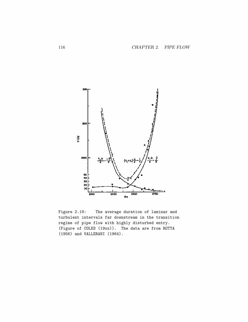
116 CHAPTER 2. PIPE FLOW
Figure 2.19: The average duration of laminar and
turbulent intervals far downstream in the transition
regime of pipe flow with highly disturbed entry.
(Figure of COLES (19xx)). The data are from ROTTA
(1956) and VALLERANI (1964).
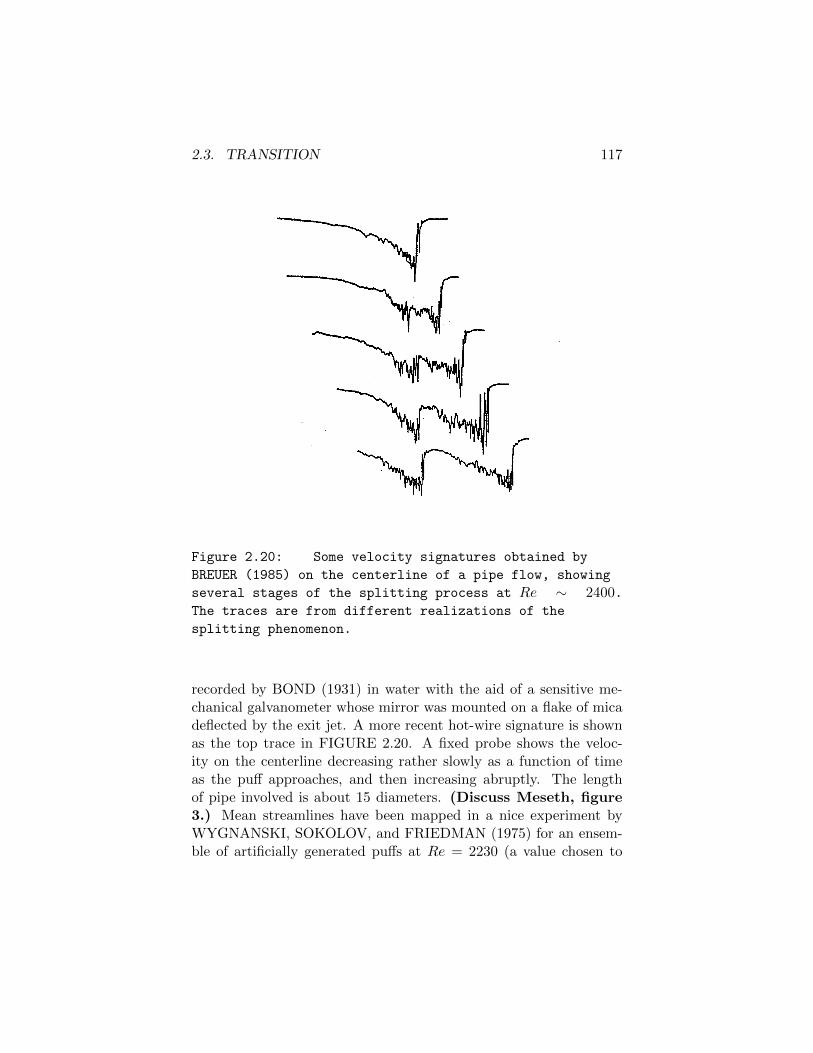
2.3. TRANSITION 117
Figure 2.20: Some velocity signatures obtained by
BREUER (1985) on the centerline of a pipe flow, showing
several stages of the splitting process at Re ∼ 2400.The traces are from different realizations of the
splitting phenomenon.
recorded by BOND (1931) in water with the aid of a sensitive me-chanical galvanometer whose mirror was mounted on a flake of micadeflected by the exit jet. A more recent hot-wire signature is shownas the top trace in FIGURE 2.20. A fixed probe shows the veloc-ity on the centerline decreasing rather slowly as a function of timeas the puff approaches, and then increasing abruptly. The lengthof pipe involved is about 15 diameters. (Discuss Meseth, figure3.) Mean streamlines have been mapped in a nice experiment byWYGNANSKI, SOKOLOV, and FRIEDMAN (1975) for an ensem-ble of artificially generated puffs at Re = 2230 (a value chosen to
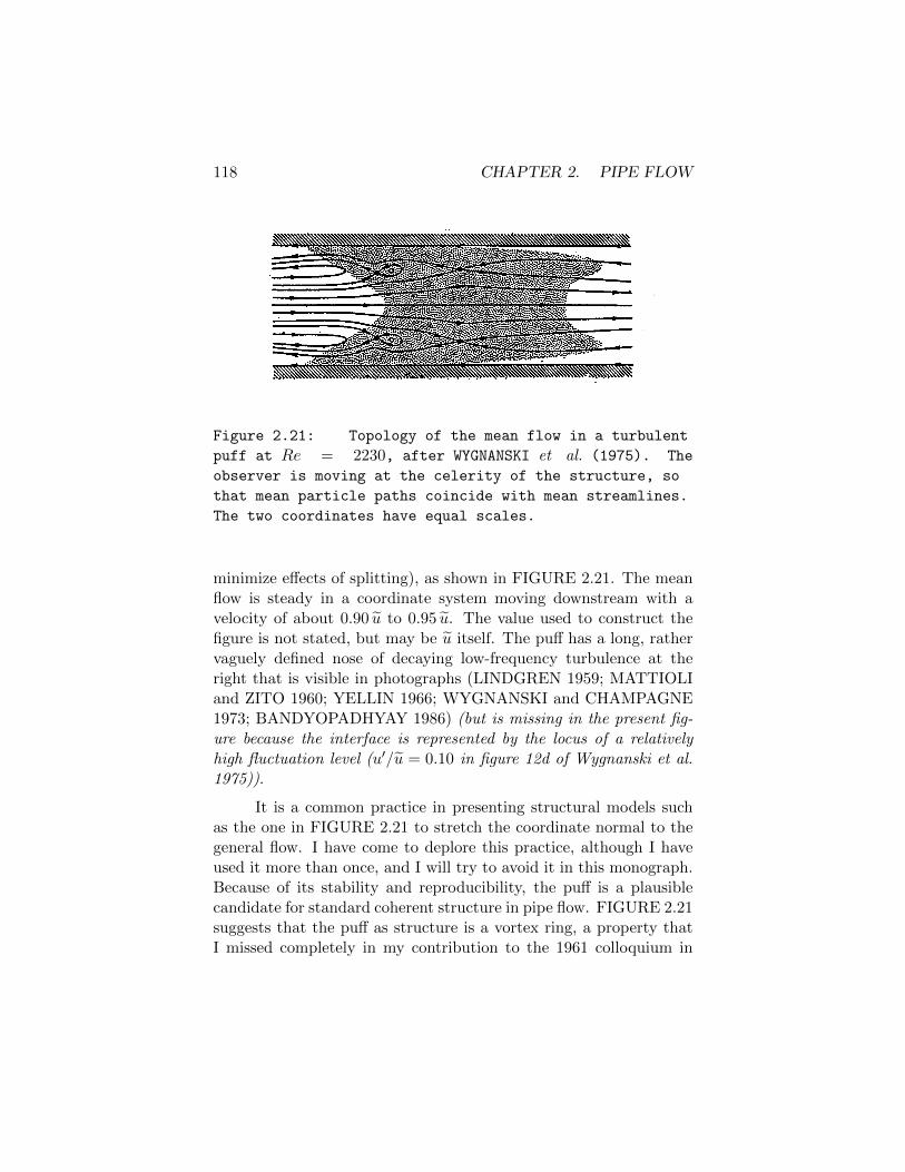
118 CHAPTER 2. PIPE FLOW
Figure 2.21: Topology of the mean flow in a turbulent
puff at Re = 2230, after WYGNANSKI et al. (1975). The
observer is moving at the celerity of the structure, so
that mean particle paths coincide with mean streamlines.
The two coordinates have equal scales.
minimize effects of splitting), as shown in FIGURE 2.21. The meanflow is steady in a coordinate system moving downstream with avelocity of about 0.90 u to 0.95 u. The value used to construct thefigure is not stated, but may be u itself. The puff has a long, rathervaguely defined nose of decaying low-frequency turbulence at theright that is visible in photographs (LINDGREN 1959; MATTIOLIand ZITO 1960; YELLIN 1966; WYGNANSKI and CHAMPAGNE1973; BANDYOPADHYAY 1986) (but is missing in the present fig-ure because the interface is represented by the locus of a relativelyhigh fluctuation level (u′/u = 0.10 in figure 12d of Wygnanski et al.1975)).
It is a common practice in presenting structural models suchas the one in FIGURE 2.21 to stretch the coordinate normal to thegeneral flow. I have come to deplore this practice, although I haveused it more than once, and I will try to avoid it in this monograph.Because of its stability and reproducibility, the puff is a plausiblecandidate for standard coherent structure in pipe flow. FIGURE 2.21suggests that the puff as structure is a vortex ring, a property thatI missed completely in my contribution to the 1961 colloquium in
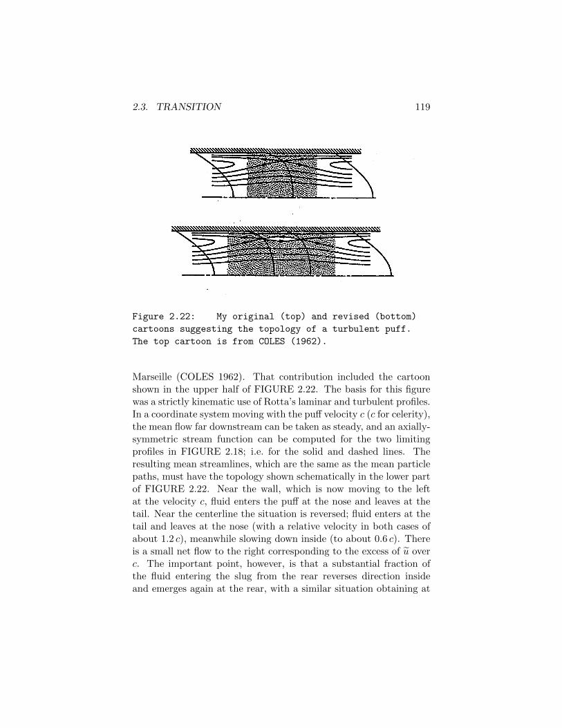
2.3. TRANSITION 119
Figure 2.22: My original (top) and revised (bottom)
cartoons suggesting the topology of a turbulent puff.
The top cartoon is from COLES (1962).
Marseille (COLES 1962). That contribution included the cartoonshown in the upper half of FIGURE 2.22. The basis for this figurewas a strictly kinematic use of Rotta’s laminar and turbulent profiles.In a coordinate system moving with the puff velocity c (c for celerity),the mean flow far downstream can be taken as steady, and an axially-symmetric stream function can be computed for the two limitingprofiles in FIGURE 2.18; i.e. for the solid and dashed lines. Theresulting mean streamlines, which are the same as the mean particlepaths, must have the topology shown schematically in the lower partof FIGURE 2.22. Near the wall, which is now moving to the leftat the velocity c, fluid enters the puff at the nose and leaves at thetail. Near the centerline the situation is reversed; fluid enters at thetail and leaves at the nose (with a relative velocity in both cases ofabout 1.2 c), meanwhile slowing down inside (to about 0.6 c). Thereis a small net flow to the right corresponding to the excess of u overc. The important point, however, is that a substantial fraction ofthe fluid entering the slug from the rear reverses direction insideand emerges again at the rear, with a similar situation obtaining at
120 CHAPTER 2. PIPE FLOW
the front. After the publication of the paper by Wygnanski et al.,it became obvious that the cartoon should be dynamic, and shouldlook like the lower half of FIGURE 2.22, this being topologicallyequivalent to FIGURE 2.21. The term vortex implies here (as itdoes in the case of the inviscid Hill spherical vortex, say) only theexistence of closed mean streamlines in a suitable moving coordinatesystem, and not necessarily the existence of a local peak in meanvorticity.
Given the present view, an explanation also presents itself forthe strong stabilizing effect of curvature noted by TAYLOR (1929).Puffs survive in a straight pipe for Re greater than about 2000, butpuffs survive in a pipe coiled to a diameter of 100D, say, only forRe greater than about 5000. I believe that in a puff the vortexring is the engine that makes the structure run. The secondary flowin the curved pipe presumably disables this engine by interferingwith the geometric and dynamic equilibrium between the puff andits environment. Note that I am answering G.I.’s question (giveref) nearly 50 years later.
2.3.4 Short account of flow in coiled pipes
Bits and pieces of circumstantial evidence can be found to suggestthat the vortex ring is (or is not) the prototype large eddy in fullydeveloped turbulent pipe flow. LINDGREN (1969) thought he rec-ognized puffs in flow at Reynolds numbers near 6000. Champagne(private communication) has verified the emergence of puffs when aninitially turbulent flow was reduced in Reynolds number from 11300to 2260 in a long diffuser, but no hard numbers are available. RU-BIN, WYGNANSKI, and HARITONIDIS (1980) suggested that thelength of plugs might be quantized in multiples of 25D, but I do notfind their evidence to be completely persuasive.
Both flow-visualization studies and data on fluctuations indi-cate that the turbulence level is relatively high at the rear of a puff,and that the transition from a laminar to a turbulent state for fluidentering the puff from the rear occurs abruptly. The fluid leaving thepuff at the front, on the other hand, undergoes a slow acceleration
2.3. TRANSITION 121
requiring at least several pipe diameters for completion, while at thesame time the turbulence becomes progressively coarser and weakeruntil it is no longer detectable. The most mysterious and challengingaspect of these observations is the fact that fluid is flowing throughthe turbulent region, entering and leaving. Another confirmed in-stance of this behavior is spiral turbulence in circular Couette flow(COLES 1965). The possibility arises of an unnatural phenomenonthat might be called anti-transition, perhaps with negative turbu-lence production, in which fluid crosses a laminar/turbulent inter-face from the turbulent to the laminar side. After some ambitiousmeasurements in spiral turbulence by C. VAN ATTA (1964) wereanalyzed to a point where the three-dimensional mean flow was ad-equately defined, as in FIGURE 2.23, it became apparent that themean flow near an anti-transition interface was in fact nearly paral-lel to the interface, and thus that the dynamical process in this flowwas a dissipative process of the conventional kind. It is therefore notconstructive to say that fluid leaves the turbulence. It is more accu-rate to say that turbulence leaves the fluid, through viscous decay,until the state can only be described as laminar. The flow in the longdownstream nose of a puff meets this condition.
2.3.5 Splitting
Another striking phenomenon discovered by Lindgren is splitting ofindividual turbulent puffs at Reynolds numbers in the lower transi-tion region (see the records in LINDGREN 1957, figures 4.7, 4.19,5.4). For x/D greater than about 200, the dimensionless frequencyfD/u has a maximum value at a Reynolds number of about 2400, asalready shown in FIGURE 2.16. On either side of the maximum theplug frequency decreases sharply, because the plug population nearthe entrance is reduced at lower Reynolds numbers by the demise,and at higher Reynolds numbers by the consolidation, of individualplugs. Rotta apparently doubted the accuracy of his data for in-termittency frequency at the lower Reynolds numbers and the moredownstream stations, because the data showed the frequency increas-ing with increasing x/D at fixed Re. He speculated that vibration
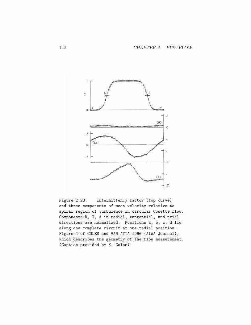
122 CHAPTER 2. PIPE FLOW
1970 D. COLES A~D C. YAi\ ATTA AIAA JOURNAL
Fig. 2 C ross section s howing mean shape of turbulent region at midlength (,•iew looking south in laboratory); radial coordinate s ljgbtly distorted for clarity. Rey nold:> number are Ro = 50,000, R ; = -5,600. i'iot e tha t a n g ular velocity of turbule n ce is mean of Wo and w; . Da!'hed line
i locus of measurements in Figs. 4-6.
ponent in the second plane is obtained, and o on. This calculation alternates between the two r array. until the velocity components no longer change (3 to 5 iteration;;) . The wire coefficients then are reviEed to correspond to the computer flow direction. and the program loop is repeated (4 to iterations).
The final im·ersion program was perfected only after more than three years of de1·elopment. It wa~ checked by processing calibration data in laminar flo"·, in which c~"C the known velocity magnitudes were reco1·ered within a fraction of 1% and the known flow angle- IYithin a fraction of 1°. A a1r plied to am pled tape data, the main program I ) Yerifie the input data format; 2) compute Xu elt numbers from voltages, 3) computes a nondin1ensional 1·ector velocity by the method already described, 4) flags each 1·ector w laminar or turbulent by a digital discrimination scheme, 5) edits the flag data for local incon ist.encies, 6) write the velocity data and flag;; on an output tape. 7) computes for each point in the pattern the ensemble mean of each 1·elocity component (with standard de,·iation, skewness. and flatness), ) compute the
L\: component of Reynolds stre-s, and 9) repeat · the lll.'!t two step after hifting the 1·elocity data forward or backward "'ithin each cycle o as to sharpen one or the other interface pojtion to a statistical discontinuity.
I ~
I
Fig. 3 Probe configuration of four hot wi r·es in double V ar-r·ay.
.I
0
- .1
.2
Fig. 4 Inte rmitleucy fa c tor (top c un·e); three components of mean veloci ty rei a ti' e t o turbule nt region (lower three cu r ves ) . Population for each point is 1667 samples . Corn ponents R. T , A in radial, tangential , a nd axial directions, r·espec~i\'ely, a r·e normalized , so that s urface ,·cloci t ies (\'iewed from turhulent region) are essen-
tinily + ).
Data ha1·e now been complete!~· proces:::cd for one radial position, ,;hown by the dashed cin:le in Fig. 2 (tape J-/0 ; r = 16. 75 in.). The intermitt{'ncy factor. mean velocities,t and Reynolds stre&"C are plotted in Figs. 4 and 5. In Fig. 6 the flow at thi radius i unwrapped , or de1·eloped, in order to
00!0
Fig. 5 Reynold;; s lt·e,.,.e,.. corre;oponding to mean flo w o f Fig!". 2, ·Land 6. Population fo•· each point is 1667 samples .
t The geometric configuration of the probe (a double 1· array rather than a double X arruy ) i:< ~uc·h that the computed radiul (axial ) velocity includes a ,;mall contribut ion from the rudial (axial) gradient of tangential veloeity. A correction in the mean for this effect can evidently be made a..: :50on as the digital data have all been proce;-:;ed to the present stage.
Figure 2.23: Intermittency factor (top curve)
and three components of mean velocity relative to
spiral region of turbulence in circular Couette flow.
Components R, T, A in radial, tangential, and axial
directions are normalized. Positions a, b, c, d lie
along one complete circuit at one radial position.
Figure 4 of COLES and VAN ATTA 1966 (AIAA Journal),
which describes the geometry of the flow measurement.
(Caption provided by K. Coles)

2.3. TRANSITION 123
and capillary forces may have caused the exit jet to break up forthe longer tubes. Rotta smoothed his original data in an effort toremove the observed increase in f . He thus missed the most remark-able transition phenomenon of all, the phenomenon of splitting ofturbulent regions of flow.
Some puff signatures observed in a flow subject to splitting areincluded in FIGURE 2.20. The data are from the master’s thesis byBREUER (1985) and were obtained in air using a hot wire on thepipe axis. The five traces are from five different events that havebeen selected from a larger population to represent various stagesof the splitting process. There is a strong impression that splittingoccurs near the trailing edge of the puff, in the region where turbu-lent fluctuations are large and may extend to include momentarilylaminar behavior.
Splitting introduces complications in any study of celerity inthe lower transition regime. One turbulent region can become two,three, four . . . regions as puffs move downstream, provided that spaceis available in the pressure field. Different observers do not agreeabout the site of this splitting. LINDGREN (1957) seems to placethe site at the front, while WYGNANSKI, SOKOLOV, and FRIED-MAN (1975) seem to place it at the rear. Quantitative informationabout splitting is rare and inconsistent. Wygnanski et al. reportup to four turbulent regions in train at a station 450D downstreamfrom a single disturbance. VALLERANI (1964) reports the samenumber at a station almost an order of magnitude farther down-stream in an apparatus having a better-developed laminar profilebut poor flow regulation. The difference may be partly a matter ofReynolds number and partly a matter of flow regulation. Valleranialso noted some variations in the length of laminar regions createdby splitting, depending on Reynolds number and on the number ofturbulent regions in train. There are evidently several importantunresolved issues involving the mechanisms that promote splittingand prevent coalescence of turbulent regions in pipe transition. Theexperiments are technically simple, and more study will probably befruitful if the right questions are asked.

124 CHAPTER 2. PIPE FLOW
Figure 2.24: Leading-edge and trailing-edge
celerities for puffs and plugs in pipe flow as measured
by several authors.
2.3.6 Celerity
Much of Lindgren’s work is concerned with the evolution of individualturbulent regions relatively near the pipe entrance, rather than withasymptotic conditions far downstream. One quantity that seems tobe quite insensitive to the details of the flow is the trailing-edge ve-locity. Lindgren obtained data in various tubes with various fluidsand entry conditions, using both optical and pressure instrumenta-tion. The measurements by various authors, shown in FIGURE 2.24,extend beyond the real transition range in both directions, so thatthe flows in questions cannot be statistically stationary in x. On theone hand, Lindgren’s observations at low values of Re confirm thatturbulence originating near the entrance tends to decay far down-stream. Consequently, his measurements of interface velocity in thisrange refer to puffs that have survived long enough to be detected attwo successive stations along the pipe (see the oscillographic recordsin Lindgren’s figures 4.6, 4.7, 4.19, 4.20, as well as his table 2.5; also
2.3. TRANSITION 125
LINDGREN 1960, figure 5). For the measurements at values of Reabove the transition range, on the other hand, a low level of inlet tur-bulence was necessary in order to observe intermittency at all. Plugsfirst appeared somewhere downstream of the entrance, probably inthe manner described by REYNOLDS (1883), and grew rapidly (seethe oscillographic records in Lindgren’s figures 4.14, 5.9, 5.10; alsoLINDGREN 1960, figures 6, 7). Provided that these plugs had notyet merged, Lindgren was also able to measure the leading-edge ve-locity shown in FIGURE 2.24. He does not comment on these datain terms of the implied rate of approach to a fully turbulent state, nordoes he provide any information about flow at quite low Reynoldsnumbers, where the relative magnitude of the two velocities shouldin principle be reversed as evidence of decay.
Leading-edge and trailing-edge velocities for puffs and plugshave been measured as a function of Reynolds number by severalinvestigators;
LINDGREN (1957)VALLERANI (1964)SARPKAYA (1966)STERN (1970)PATERSON and ABERNATHY (1972)WYGNANSKI and CHAMPAGNE (1973)MESETH (1974)TEITGEN (1980)ZALZAL et al. (1994)
with the results recorded in FIGURE 2.24. The quantities plotted inthe figure are essentially phase velocities, or more accurately veloci-ties at constant phase. Early experimenters, particularly Favre (ref)and Kovasznay (ref), tried to give such velocities a special meaningby choosing the French word celerite, rather than the more con-ventional word vitesse. In this monograph, I will consistently usethe word celerity to refer to velocities associated with structure andphase. The figure leaves no doubt that different processes are oc-curring in the upper and lower parts of the transition regime, witha divide at about Re = 2400. Below this divide, turbulent regions
126 CHAPTER 2. PIPE FLOW
have approximately constant length and therefore essentially a sin-gle celerity, which is most easily measured at the trailing interface.The measurement may be hampered by splitting. Above the divide,the leading interface moves faster than the trailing one if space isavailable, as first noted by Lindgren. Hence celerity at these higherReynolds numbers is usually measured in a different mode. Laminarflow is set up in a pipe with smooth entry, and the time interval ismeasured between a local artificial disturbance and the associatedresponse at one or more downstream stations.
The measurements in FIGURE 2.24 suffer from deficienciesthat raise the question of reproducibility among the various exper-iments. In part this is because of different detection schemes forthe interfaces. More generally, however, the data may be subject toambiguity coming from at least four sources.
First, the entry flow should be smooth and quiet, and the lam-inar flow in the test region should have a fully developed parabolicprofile, with x/D at least equal to Re/16 at the site of any pro-grammed disturbance. When this condition is not met, the shape ofthe laminar-turbulent interfaces will imitate the shape of the laminarprofile and will depend on x/D (WYGNANSKI 1970; WYGNANSKIand CHAMPAGNE 1973; TEITGEN 1975). Moreover, the properreference velocity for celerity is no longer the theoretical maximumvelocity 2 u for the parabolic profile, but rather the actual maximumvelocity at a given station (WYGNANSKI and CHAMPAGNE 1973).In a short pipe, this velocity may be closer to u than to 2 u, and mayvary over the observation distance. Measurements of celerity at highReynolds numbers have a particularly ad hoc quality in short pipeswhen transition occurs spontaneously or is triggered artificially inthe developing laminar boundary layer (LINDGREN 1957; WYG-NANSKI 1970; WYGNANSKI and CHAMPAGNE 1973). In suchcases it is relevant that the boundary layer in the pipe has thicknessδ ∼ (νx/u∞)1/2. In any event, far downstream the concept of celerityeventually has no meaning outside the transition range of Reynoldsnumbers. I therefore have serious doubts about the usefulness of themeasurements in FIGURE 2.24.
Second, the formation time should be excluded from measure-
2.3. TRANSITION 127
ments of celerity by making observations at two stations, each ofwhich is sufficiently far downstream for the structure of the turbulentregion to become independent of details of the formation process. Insome cases (VALLERANI 1964, MESETH 1974), the response wasobserved at only one downstream station so that the formation pro-cess for the turbulent region was not excluded from the measuredtime intervals.
Third, the disturbance should be of short duration, especiallyin the lower transition regime, where a puff passes a fixed station in atime 15D/u. In some cases (Gilbrech & Hale 1965, Sarpkaya 1966),the duration of the disturbance was probably too long, at least at lowReynolds numbers, where an almost impulsive disturbance is calledfor.
Finally, close attention must be paid to flow regulation. If themean velocity is not regulated by the experimenter, say by use ofa sonic orifice, a positive-displacement pump, or a massive flow re-striction, it will be regulated by the experiment, and will vary withthe relative fractions of laminar and turbulent flow at each instant.This transient effect is probably less important for intermittent flowwith disturbed entry at low Reynolds numbers than for intermittentflow with smooth entry at higher Reynolds numbers. In cases whereenough information is available to judge the matter, poor flow reg-ulation is more the rule than the exception. Lindgren, for example,recognized that his flow circuit was unstable and that a limit cyclecould occur in his apparatus.
PRANDTL and TIETJENS (19xx, pp. x) give a glimpse ofsome data for such an oscillation from experiments at Gottingen.They cite Couette’s experience as a precedent, although I believethat Couette was describing intermittency of the normal kind. Otherevidence in the literature (Brockmann, Mickelson) suggests thatthe oscillation is not unusual. I am surprised that there are no hardnumbers, although the conditions must be quite special and mayinclude restricted ranges for Re and L/D as well as a delicate controlof disturbances at the pipe entry. (Pantulu, Jenkinson.) There iseven a standard for this relaxation process. Suppose that the flowstate in a pipe is fully turbulent, and let the flow be subjected to
128 CHAPTER 2. PIPE FLOW
a gradual or abrupt increase in pipe diameter from D1 to D2. TheReynolds number will decrease from Re1 to Re2 = (D1/D2)Re1.Laufer (ref) and Sibulkin (ref) studied such flows for the case of agradual area change, with Re1 > 3000 and Re2 < 2000.
Transition in pipe flow is intermittent. Pipe or channel flow,like the round wake (check), is special in that the Reynolds numberis constant in the flow direction. A higher Reynolds number doesnot refer to a more downstream location in a given flow, but toa physically different flow in parameter space. This fact in turnmakes the length-to-diameter ratio L/D an important dimensionlessparameter.
2.4 Turbulent flow in a smooth pipe
2.4.1 Early work
Fundamental research on turbulent pipe flow goes back to the period1840–1860 and the work of Hagen, Hagenbach, and Darcy. The con-tributions by early civil engineers are well summarized in the shorthistory by ROUSE and INCE (1957). This work often involved theeffect of roughness in commercial pipes, especially after long use, andthe problem of roughness was very slow in coming under control.Fundamental research on pipe flow also requires an understanding ofthe effects of entrance conditions, especially for short pipes. Someof these effects are known, and others can be inferred by examiningdiscrepancies among available measurements of friction and otherquantities in turbulent flow. The issue once again is whether or notturbulent pipe flow tends far downstream to a unique state, as itmust if pipe flow is to be a fit subject for fundamental research onthe mechanisms of turbulence.
For flow in a smooth pipe far downstream from a noisy en-trance, the empirical evidence, even in the transition regime, appearsto be that the wall friction (i.e., the pressure gradient) is determineduniquely by the fluid properties, the pipe diameter, and the flow rate(i.e., the mean velocity). Engineers today understand that the ex-
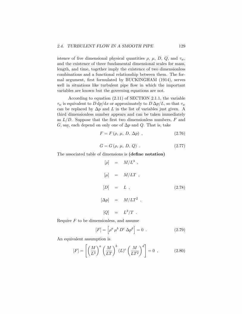
2.4. TURBULENT FLOW IN A SMOOTH PIPE 129
istence of five dimensional physical quantities ρ, µ, D, Q, and τw,and the existence of three fundamental dimensional scales for mass,length, and time, together imply the existence of two dimensionlesscombinations and a functional relationship between them. The for-mal argument, first formulated by BUCKINGHAM (1914), serveswell in situations like turbulent pipe flow in which the importantvariables are known but the governing equations are not.
According to equation (2.11) of SECTION 2.1.1, the variableτw is equivalent to D dp/dx or approximately to D∆p/L, so that τwcan be replaced by ∆p and L in the list of variables just given. Athird dimensionless number appears and can be taken immediatelyas L/D. Suppose that the first two dimensionless numbers, F andG, say, each depend on only one of ∆p and Q. That is, take
F = F (ρ, µ, D, ∆p) , (2.76)
G = G (ρ, µ, D, Q) . (2.77)
The associated table of dimensions is (define notation)
[ρ] = M/L3 ,
[µ] = M/LT ,
[D] = L , (2.78)
[∆p] = M/LT 2 ,
[Q] = L3/T .
Require F to be dimensionless, and assume
[F ] =[ρa µb Dc ∆pd
]= 0 . (2.79)
An equivalent assumption is
[F ] =
[(M
L3
)a (MLT
)b(L)c
(M
LT 2
)d]= 0 , (2.80)
130 CHAPTER 2. PIPE FLOW
or [Ma+b+d L−3a−b+c−d T−b−2d
]= 0 . (2.81)
Three simultaneous algebraic equations are obtained for the fourexponents;
a+ b + d = 0 ,
−3a− b+ c − d = 0 , (2.82)
b + 2d = 0 .
Let one exponent, say d, be treated as given. These equations thenhave the one-parameter solution
a = d ,
b = −2d , (2.83)
c = 2d .
(Comment that the Π theorem involves the matrix prop-erties of systems like equations (2.82).) Consequently, equa-tion (2.79) must have the form
[F ] =
[(ρD2∆p
µ2
)d]= 0 , (2.84)
in which the value of d is immaterial, since any ratio or product ofdimensionless combinations or their powers is also dimensionless. Asimilar treatment of equation (2.77) for G leads to
[G] =
[(ρQ
µD
)b]= 0 . (2.85)
The exponents d and b, since they are associated with dimensionlessscales and not with physical variables, can play no physical role. Thethree dimensionless parameters for pipe flow therefore emerge fromBuckingham’s analysis as
L
D,
ρQ
µD,
ρD2∆p
µ2. (2.86)
2.4. TURBULENT FLOW IN A SMOOTH PIPE 131
The second of these is equivalent to the Reynolds number Re,according to equations (2.15) and (2.19), and the third is equivalentto the product Re2Cf . It is possible, and may even be useful, tothink of pipe flow as a nonlinear fluid operator whose primary inputvariable is a flow rate Q or u and whose primary output variableis a pressure difference ∆p or τw, or conversely. It is no accidentthat these input and output variables were deliberately isolated byReynolds in the original definitions (2.76) and (2.77). This choicealso amounts to defining three characteristic velocities u, (τw/ρ)1/2,and ν/D, whose ratios can be taken as uD/ν and τwD
2/ρν2.
By common consent, the standard combinations have by nowbecome Cf and Re, where
Cf =τw
ρu2/2(2.87)
and
Re =uD
ν. (2.88)
The implied functional relationship Cf = Cf (Re) is capable of col-lapsing information from numerous sources into a clear and widelyaccepted system of description. For laminar flow, this system is theequation Cf = 16/Re already derived in SECTION 2.1.2. The nextseveral sections describe one possible system for turbulent flow. Forboth laminar and turbulent regimes of flow, however, the existenceof any system was recognized only after the major conceptual ad-vance that underlies the previous discussion of this section; namely,development of the art of dimensional analysis.
Reynolds. A classical paper by REYNOLDS (1883) is fre-quently cited in this context but, I suspect, not frequently read. Inone part of his paper, Reynolds used some imaginative flow visual-ization in water to observe and describe intermittent transition in acircular pipe in terms of the properties of the internal flow, ratherthan the properties of a liquid jet at the exit (see SECTION 2.3.1).By observing the behavior of filaments of dye, he found that the on-set of transition within the pipe was local and sudden and occurredat essentially the same value of uD/ν for three glass pipes of different

132 CHAPTER 2. PIPE FLOW
diameters. The pipes had a faired inlet and a quiet entrance flow.When inlet disturbances were reduced to a practical limit, the con-stant value of uD/ν in question was about 12,800. Because the pipeswere far too short to provide a fully developed parabolic profile, itis clear that Reynolds was observing the effects of boundary-layerinstability in the development region, and that no special mean-ing ought to be attached to the value quoted for uD/ν. In fact,EKMAN (1911) repeated some of Reynolds’ work, using Reynolds’original apparatus, and verified a strong sensitivity of transition toupstream disturbance level. What is of permanent value in this partof Reynolds’ paper is his observation that both of the primary exper-imental variables, the flow rate and the pressure gradient, could beexpressed in dimensionless form, at least for the limited purpose ofdescribing the onset of transition. It is not at all clear that Reynoldsintended this observation to apply for more general purposes.
In the remainder of his paper, Reynolds reported new data onfriction for water flowing in two drawn lead pipes. He avoided thedevelopment problem by carefully tapping his pipes for local pres-sure measurements well downstream. The entrance flow was delib-erately made noisy, because his objective in this part of his studywas to establish conditions for which all disturbances would decayand laminar pipe flow could be described as unconditionally stable.FIGURE 2.25 reproduces Reynolds’ results, as displayed in his dia-gram 2. The abscissa i = (dp/dx)/ρg is the quantity tabulated byReynolds and is inadvertently dimensionless. If the local static pres-sure p is measured by observing the height h reached by the workingliquid in a manometer tube connected to a hole in the pipe wall, thenp = ρgh and dp/dx = ρgdh/dx = ρgi. The quantity i is commonlycalled the hydraulic grade, hydraulic slope, or hydraulic gradient bycivil engineers.
In presenting his data, Reynolds twice displayed a generic for-mula relating pressure drop to flow rate. This formula is essentiallythe form Re2Cf = g(Re) already mentioned. However, Reynolds’version of the formula is not strictly dimensionless and as writtenis valid only for water. Where I have Re, Reynolds has ν0Re, andwhere I have Re2Cf , Reynolds has (2ν2
0/g)Re2Cf , with ν0 the kine-

2.4. TURBULENT FLOW IN A SMOOTH PIPE 133
10-4 10-3 10-2 10-1 100 101100
101
102
103
+
++
+ ++++++++++++
i
v
Figure 2.25: Diagram 2 of the paper by REYNOLDS
(1883), reproduced with the aid of his tables III--V.
The abscissa i = dh/dx = (dp/dx)/ρg is the dimensionless
local pressure gradient. The ordinate v is the mean
velocity in cm/sec.

134 CHAPTER 2. PIPE FLOW
103 104 105 106 107 108102
103
104
105
R e2C f
R e
Figure 2.26: The previous FIGURE 2.25 made
dimensionless by following Reynolds’ instructions.
Reynolds described this figure but did not display it.
matic viscosity of water at 0 ◦C and g the acceleration of gravity.Reynolds commented more than once that the dimensional data forhis two pipes, as well as data obtained by other investigators, couldbe superposed by a suitable displacement in logarithmic coordinates,and he gave explicit rules for calculating the necessary displacements.For example, log u should be replaced by log u+logD− log ν+log ν0.I have applied these rules to the data in FIGURE 2.25, omitting theconstant dimensional factors ν0 and g, to obtain FIGURE 2.26. Iconsider it truly remarkable that Reynolds did not himself carry outthe calculations, and thus did not arrive at FIGURE 2.26, whichwould have revealed at one stroke the power of dimensional analysisand the importance of what is now called the Reynolds number.
The consequences of this omission were profound. Reynolds’paper had no real impact on his contemporaries. Thirty years passed,and more than fifty papers on turbulent pipe flow, before the last step
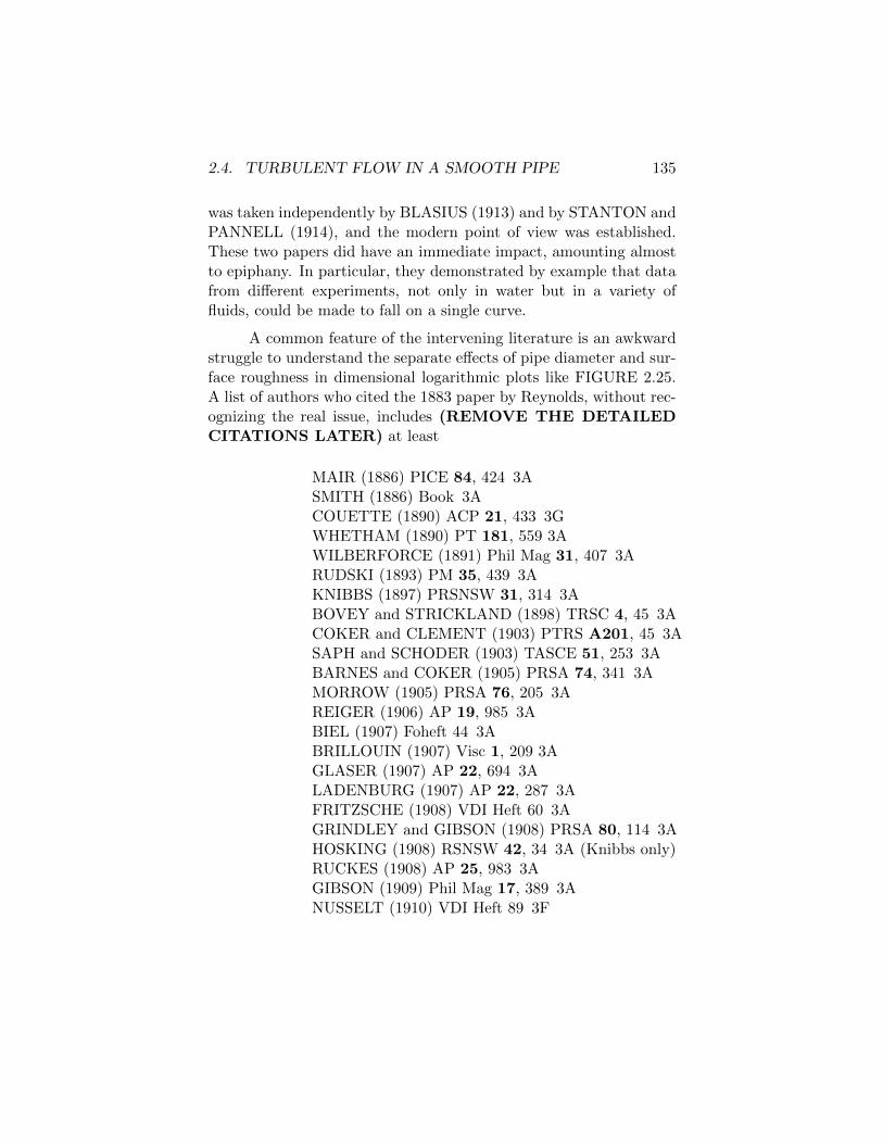
2.4. TURBULENT FLOW IN A SMOOTH PIPE 135
was taken independently by BLASIUS (1913) and by STANTON andPANNELL (1914), and the modern point of view was established.These two papers did have an immediate impact, amounting almostto epiphany. In particular, they demonstrated by example that datafrom different experiments, not only in water but in a variety offluids, could be made to fall on a single curve.
A common feature of the intervening literature is an awkwardstruggle to understand the separate effects of pipe diameter and sur-face roughness in dimensional logarithmic plots like FIGURE 2.25.A list of authors who cited the 1883 paper by Reynolds, without rec-ognizing the real issue, includes (REMOVE THE DETAILEDCITATIONS LATER) at least
MAIR (1886) PICE 84, 424 3ASMITH (1886) Book 3ACOUETTE (1890) ACP 21, 433 3GWHETHAM (1890) PT 181, 559 3AWILBERFORCE (1891) Phil Mag 31, 407 3ARUDSKI (1893) PM 35, 439 3AKNIBBS (1897) PRSNSW 31, 314 3ABOVEY and STRICKLAND (1898) TRSC 4, 45 3ACOKER and CLEMENT (1903) PTRS A201, 45 3ASAPH and SCHODER (1903) TASCE 51, 253 3ABARNES and COKER (1905) PRSA 74, 341 3AMORROW (1905) PRSA 76, 205 3AREIGER (1906) AP 19, 985 3ABIEL (1907) Foheft 44 3ABRILLOUIN (1907) Visc 1, 209 3AGLASER (1907) AP 22, 694 3ALADENBURG (1907) AP 22, 287 3AFRITZSCHE (1908) VDI Heft 60 3AGRINDLEY and GIBSON (1908) PRSA 80, 114 3AHOSKING (1908) RSNSW 42, 34 3A (Knibbs only)RUCKES (1908) AP 25, 983 3AGIBSON (1909) Phil Mag 17, 389 3ANUSSELT (1910) VDI Heft 89 3F
136 CHAPTER 2. PIPE FLOW
UNWIN (1910) Enc Brit 3BOSE and BOSE (1911) PZ 12, 126 3AEKMAN (1911) AMAF 6, 1 3GRONCERAY (1911) Ann CP 22, 107 3ASOENNECKEN (1911) Foheft 108, 109 3FCAROTHERS (1912) PRSA 87, 154 3ALECHNER (1913) AP 42, 614 3AGIBSON (1914) PIME 201, 201 3AKOHLRAUSCH (1914) AP 44, 297 3ARAPP (1914) Phys Rev 2, 363 3A
A similar list can be constructed of authors who wrote aboutpipe flow in this period 1883–1913 but did not cite the 1883 paperby Reynolds. It is probably not a coincidence that this second listcontains almost all of the papers that report measurements withair or some other gas as a working fluid (check). Apparently theperception of Reynolds’ ideas by his contemporaries, and perhapsby Reynolds himself, notwithstanding the remarks in his sections36 and 37, was the one already stated; namely, that these ideasapply only for water, and that the combination uD/ν plays a roleonly in connection with the onset of transition, and not as a genericdimensionless variable.
Several of these early papers will be mentioned again in SEC-TION 2.4.3, where the available measurements of friction will bereviewed for the classical case of fully developed turbulent flow ina smooth circular pipe. The Encyclopaedia Britannica article byUnwin, in particular, is a good account of the shapeless empiricismpracticed by civil and mechanical engineers of the time. References toother early work can be found in the papers by Biels, Fritzsche, andBlasius, and in surveys by OMBECK (1914), DAVIES and WHITE(1929), DREW, KOO and McADAMS (1932), and KEMLER (1933).(Check GUMBEL 1913, SCHILLER 1925). The paper by NUSSELT(1910) approaches, but does not quite achieve, dimensional comple-tion.
Karman. The paper by BOSE and BOSE (1911; for completedata, see BOSE and RAVERT 1909) deserves particular attention foranother reason. These authors determined the time T required for
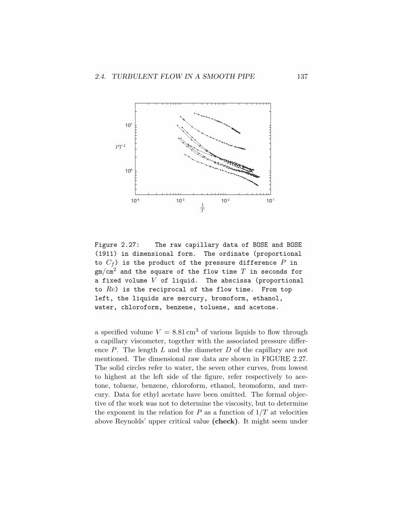
2.4. TURBULENT FLOW IN A SMOOTH PIPE 137
10-4 10-3 10-2 10-1
106
107
P T 2
1T
Figure 2.27: The raw capillary data of BOSE and BOSE
(1911) in dimensional form. The ordinate (proportional
to Cf) is the product of the pressure difference P in
gm/cm2 and the square of the flow time T in seconds for
a fixed volume V of liquid. The abscissa (proportional
to Re) is the reciprocal of the flow time. From top
left, the liquids are mercury, bromoform, ethanol,
water, chloroform, benzene, toluene, and acetone.
a specified volume V = 8.81 cm3 of various liquids to flow througha capillary viscometer, together with the associated pressure differ-ence P . The length L and the diameter D of the capillary are notmentioned. The dimensional raw data are shown in FIGURE 2.27.The solid circles refer to water, the seven other curves, from lowestto highest at the left side of the figure, refer respectively to ace-tone, toluene, benzene, chloroform, ethanol, bromoform, and mer-cury. Data for ethyl acetate have been omitted. The formal objec-tive of the work was not to determine the viscosity, but to determinethe exponent in the relation for P as a function of 1/T at velocitiesabove Reynolds’ upper critical value (check). It might seem under
138 CHAPTER 2. PIPE FLOW
the given conditions that there is no presentation that will collapsethe Bose data to a single curve. However, KARMAN, while stillat Gottingen, pointed out such a presentation (1911). His originalshort paper lacks figures and is otherwise opaque, and apparentlyattracted no attention. The matter is more clearly presented in apassage in his tutorial volume Aerodynamics (1954), where both theproblem and its solution are illustrated by figures.
Recall the friction coefficient Cf and Reynolds number Re de-fined by equations (2.20) and (2.19) respectively. Three auxiliaryequations, (2.15) for u, (2.11) for τw, and the definition of the flowrate Q,
Q =V
T, (2.89)
are needed. From these, it is easy to verify the identities (define Cf )
ρV 2/3
µT=π
4
(D
V 1/3
)Re (2.90)
andgPT 2
ρV 2/3=
32
π2
(LV 4/3
D5
)Cf , (2.91)
together with their product
gPT
µ=
8
π
(LV
D4
)Cf Re . (2.92)
In each of these equations, the quantities on the left are known ex-perimentally. The dimensionless combinations in parentheses on theright are not known, but are not needed to make Karman’s point.Note that the last equation makes the product PT constant for ideallaminar flow, as stated by Poiseuille in the first of his laws.
Karman worked out the variables on the left in these dimen-sionless relationships by an argument based on proportional scalingof various terms in the momentum equation. A length scale wasneeded for this argument. There are three obvious candidates, L,D, and V 1/3, all of which are constant for the whole course of theexperiments. Karman used V 1/3, since this is the only length that

2.4. TURBULENT FLOW IN A SMOOTH PIPE 139
gPT2
pV2/3
10-1
pV2/3
µT
101 102
FIGURE 3.35 The data of Figure 3.34 after reduction to dimensionless form by KARMAN (1911). Handbook values have been used for density and viscosity. The capillary tube was apparently quite short, with L/ D perhaps about 15, and the apparatus is therefore usable only for relative viscometry.
Figure 2.28: The data of the previous FIGURE 2.27
after reduction to dimensionless form following KARMAN
(1911). Handbook values have been used for density
and viscosity. The capillary tube was apparently quite
short, with L/D perhaps about 60, and the data are
therefore usable only for relative viscometry.
is specified numerically. He showed that the data for different flu-ids then defined a single curve, as displayed in FIGURE 2.28. Sucha display is not quite viscometry, because it cannot be reduced tostandard dimensionless variables Cf and Re as long as L and D areunknown. However, if µ is known for any one liquid, such as water,the tabulated data can be used to infer µ for each of the other liquids.
This contribution by Karman required little in the way of equa-tions or models except for overall mass and momentum balance. Itdoes not involve empirical constants and makes no distinction be-tween laminar and turbulent flow. It is therefore an impressive earlyillustration of the power and beauty of the dimensional art. More-over, later developments in modeling applied to capillary-tube vis-
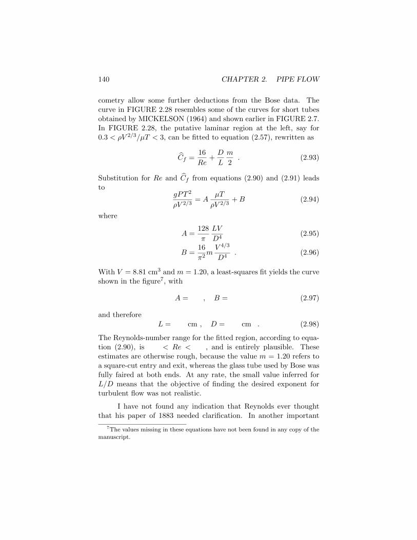
140 CHAPTER 2. PIPE FLOW
cometry allow some further deductions from the Bose data. Thecurve in FIGURE 2.28 resembles some of the curves for short tubesobtained by MICKELSON (1964) and shown earlier in FIGURE 2.7.In FIGURE 2.28, the putative laminar region at the left, say for0.3 < ρV 2/3/µT < 3, can be fitted to equation (2.57), rewritten as
Cf =16
Re+D
L
m
2. (2.93)
Substitution for Re and Cf from equations (2.90) and (2.91) leadsto
gPT 2
ρV 2/3= A
µT
ρV 2/3+B (2.94)
where
A =128
π
LV
D4(2.95)
B =16
π2mV 4/3
D4. (2.96)
With V = 8.81 cm3 and m = 1.20, a least-squares fit yields the curveshown in the figure7, with
A = , B = (2.97)
and therefore
L = cm , D = cm . (2.98)
The Reynolds-number range for the fitted region, according to equa-tion (2.90), is < Re < , and is entirely plausible. Theseestimates are otherwise rough, because the value m = 1.20 refers toa square-cut entry and exit, whereas the glass tube used by Bose wasfully faired at both ends. At any rate, the small value inferred forL/D means that the objective of finding the desired exponent forturbulent flow was not realistic.
I have not found any indication that Reynolds ever thoughtthat his paper of 1883 needed clarification. In another important
7The values missing in these equations have not been found in any copy of themanuscript.

2.4. TURBULENT FLOW IN A SMOOTH PIPE 141
paper on turbulent flow (REYNOLDS 1895), he did no more thanremove the dimensional factor ν0 in Re and propose a value of 1900–2000 as an upper limit for unconditional stability of laminar pipeflow. Reynolds also let pass opportunities to influence the presen-tation of data in the papers by Coker and Clements and by Barnesand Coker, both of which deal only with dimensional data, and bothof which bear a note “communicated by O. Reynolds.” I am told byPhilip Saffman that communication of a paper to a journal of theRoyal Society through a fellow (a requirement now abolished) meantonly that the paper was believed by the fellow to be written in En-glish, and did not imply any judgment about the scientific merit ofthe work.
This evidence presented so far does not mean that the engi-neering community in 1883, and for three decades thereafter, wasunready for the concept of dimension. The published record on thereception of Reynolds’ ideas has been explored by ROUSE and INCE(1934) and by ROTT (1990, 1992). These authors point out thatRAYLEIGH, in several short publications between 1892 and 1915,showed with professional facility that dimensional analysis, which hecalled dynamical similarity, could be applied to a great variety ofphysical problems. The first of these papers dealt specifically withReynolds’ formula for pipe flow. Reynolds himself made skillful useof modeling laws in his paper of 18xx on lifeboats, where he citedFroude as a pioneer, and in his paper of 18xx on flow in estuaries.He may not have thought of models in connection with pipe flow,although one such flow can certainly be taken as a model for an-other. The contribution by Karman has already been described atlength. PRANDTL (1905) used dimensional reasoning as a tool in hisboundary-layer theory, and a later paper by PRANDTL (1910) cer-tainly influenced the work of Blasius, just as the papers by Rayleighcertainly influenced the work of Stanton. (Mention Froude?) Itwas SOMMERFELD (1908) who proposed using the term Reynoldsnumber (Reynolds’sche Zahl) for the quantity uD/ν, thus estab-lishing a practice of naming dimensionless numbers that has sinceevolved in unpredictable directions. The method of dimensions waseventually provided with an axiomatic foundation, in Rott’s phrase,

142 CHAPTER 2. PIPE FLOW
102 103 104 105 10610-3
10-2
10-1
C f
Re
Figure 2.29: Reynolds’ pipe data in standard
dimensionless variables. The curve at the right is
faired through Nikuradse’s data. The low values of
Cf for turbulent flow may be caused by imperfect
calibration of the flowmeter.
in the definitive paper by BUCKINGHAM (1914). I think that thesematters are important enough to deserve the attention of analyticalhistorians of science who have the resources to reach the unpublishedrecord. The evolution of the Reynolds number is also worth studyas part of a larger development of the time, which was the slow anddifficult emergence of applied mathematics from pure mathematicsas a separate and eventually homologous discipline.
Finally, to close this discussion, the friction measurements byReynolds are plotted in standard form as Cf (Re) in FIGURE 2.29.The scatter is probably caused mainly by difficulties in manual reg-ulation of supply pressure in a flow system connected directly to thebuilding water supply some of the values of Cf for turbulent flow arelow by 15 to 25 percent, perhaps because of imperfect calibration of
2.4. TURBULENT FLOW IN A SMOOTH PIPE 143
the flowmeter.
By contrast with the case of the Reynolds number, dimen-sionless combinations equivalent to the definition (2.87) for the fric-tion coefficient in pipe flow were introduced very early (look upChezy). The rationale was and is mainly philosophical. Experi-ence shows that the pressure drop for turbulent flow in large pipesis roughly proportional to the square of the velocity, so that the ra-tio (dp/dx)
/ρu2 is nearly a constant. The reduction of empirical
knowledge to a constant is of itself valuable evidence of order. How-ever, notation has varied widely, and still does. Several authors haveused −Ddp/dx or −Rdp/dx as numerator in equation (2.87) ratherthan −(D/4)dp/dx = τw, denoting the resulting dimensionless com-bination by λ or ψ. The factor 1/2 in the denominator was alsosometimes omitted. In defining the Reynolds number, some authorsused R rather than D, and at least one author substituted uc for u.UNWIN (1910), in his Encyclopaedia Brittanica article, used the def-inition (2.87) but the symbol ζ. It is common to see in the literatureof mechanical and civil engineering the symbol f , known as the Fan-ning friction factor, for what is here called Cf (Fanning himself usedthe symbol m). It is worth noting that the quantity D/4 in equation(2.11) coincides, by accident or otherwise, with the hydraulic radius,if this is defined as the ratio of wetted cross-sectional area to wettedcircumference for non-circular channels, closed or open. I have notbeen able to discover why this definition was originally formulatedso that the hydraulic radius for a circular pipe is not the same as thegeometric radius. (See Prandtl and Tietjens.)
Turbulent flow in pipes has been studied from two points ofview, beginning about 1850. Civil engineers of the time were oftenconcerned with hydraulic aspects of the problem and with design ofefficient conduits for water distribution, sewage or storm-water col-lection, and chemical process engineering? Their field installationstend to be large, with rough surfaces and with numerous joints,bends, elbows, and tees. Such conduits may not always run full.Direct field measurements of friction in such conduits are a betterguide to performance than estimates derived by extrapolation froma remote classical base. Technical data of this kind have been col-

144 CHAPTER 2. PIPE FLOW
lected by (refs.). In general, however, civil engineers tend not to beproducers of basic information. One exception was DARCY (1858),who was a half century or more ahead of his time. He made carefulmeasurements of the mean-velocity profile in large conduits havingvarious degrees of roughness and invented the defect law. This lawwas also proposed independently by (refs.). It was finally establishedfirmly by systematic profile measurements by NIKURADSE (1933)in rough pipes.
2.4.2 The Nikuradse problem
The measurements that for 60 years have been taken to be definitivefor turbulent flow in smooth and rough pipes were published in 1932and 1933 in a remarkable pair of papers by J. Nikuradse. The workwas done at Gottingen under the direction of Prandtl, as was anearlier thesis (1926) that is seldom cited. The issue in the thesis wassecondary flow in uniform ducts having various cross sections; rectan-gular, trapezoidal, triangular; circular shaft with keyway. The dataconsisted mostly of contours of constant axial velocity. Nikuradseapparently also worked on smaller problems, such as laminar flowdevelopment in the entrance region of a circular tube (see figure xof PRANDTL and TIETJENS 19xx), but none of this work waspublished in usable form. (What about Tollmien-Schlichtinginstability?)
The important contribution by Nikuradse in the 1932 paperwas a systematic study of the mean-velocity profile in smooth pipesover a large range of Reynolds number. These measurements are arefreshing counter-example to a description of the scientific methodsometimes given to beginning students: form a hypothesis; test thehypothesis; accept, revise or reject the hypothesis. Prandtl had nohypothesis; or, if he did, it was overtaken by the events describedin SECTION X.8 I think that Prandtl simply believed that prop-erly constructed experiments could not fail to lead to new and im-portant conclusions about turbulent flow. This belief was certainlycorrect, because it led directly to the logarithmic profile. An im-
8Unclear reference, possibly to a section not completed.
2.4. TURBULENT FLOW IN A SMOOTH PIPE 145
portant question about the measurements, first raised publicly byMILLER (1949), concerns an unexplained discrepancy between themean-velocity profiles as plotted in figure 15 of Nikuradse’s prelimi-nary paper of 1930 and in figure 24 of his final paper of 1932. Thediscrepancy is also apparent from an examination of tables 2 and 3of the latter paper. Miller was concerned with the need to describethe profile accurately in and near the sublayer in studies of heat andmass transfer (see SECTIONS X and Y).9
Miller in 1946 unsuccessfully sought an explanation of the dis-crepancy from Nikuradse, Prandtl, and von Karman. A secondeffort, which travelled the route Miller-Rouse-Prandtl-Wieghardt-Nikuradse and back, established that Nikuradse had in fact alteredhis data for the mean velocity profile by adding 7 units to the dimen-sionless abscissa y+. The effect was to portray the viscous sublayermore realistically by ensuring that the measured velocity never fellabove the linear line inferred from the wall friction. Prandtl remarkedlater that the correction was justified, but the failure to describe itwas not. Nevertheless, Miller maintained in his 1949 paper that therewas in fact no evidence for the existence of a sublayer, although am-ple evidence was provided a little later by several other sources.
The discrepancy is sometimes described as a crude correctionfor probe–wall interference. It amounted to deletion of the two pointsnearest the wall in each profile, which scatter badly, and an increaseof seven units in the coordinate yuτ/ν for the remaining data. Thisshift is in fact obvious from a comparison of the tabulated dimen-sional and dimensionless data, as is a dislocation in the first threeentries for ϕ in Nikuradse’s table 3 for the case Re = 1.11 × 10⁶.The profiles were measured in a plane 0.01 to 0.02 cm downstreamfrom the square-cut pipe exit, where a cylindrical water jet emergedinto a confined water-filled chamber. This technique may be a relictof the thesis research. Nikuradse’s 1932 paper describes some dataobtained near the pipe wall with probes of different diameters, butdoes not justify or apply the implied correction, and I have not beenable to make any sense of his description.
9Sections evidently not completed.
146 CHAPTER 2. PIPE FLOW
The reason for Miller’s initial difficulty was that Prandtl in1946 no longer recognized Nikuradse, for a reason not related tothe pipe measurements. In 1934, Nikuradse, perhaps driven to anuncommon level of hubris by compliments about his research onpipe flow, and inspired by Hitler’s assumption of power in Germany,attempted through a putsch to replace Prandtl as director of theKaiser-Wilhelm-Institute at Gottingen. There was a brief confronta-tion, which rapidly became a test of strength between other partiesin the German political structure. At the end of a “mad and dan-gerous brawl,” as Wieghardt puts it, Prandtl was confirmed in hisposition and Nikuradse was exiled to a post as dozent at the Technis-che Hochschule at Breslau. These events are described very briefly inthe historical article by OSWATITSCH and WIEGHARDT (1988).This history is not complete, and further information is obtainedonly with great difficulty. Witnesses are few and becoming fewer,and the career of Nikuradse at the Kaiser-Wilhelm Institute is stilla source of embarrassment there.
In 1942, Nikuradse published two monographs for the Germanair force, neither of which can be taken at face value. The first,on laminar boundary layers, claims to be a publication of data ob-tained by Nikuradse at Prandtl’s institute at Gottingen in 1933. Fivevelocity profiles are tabulated in his table 6 and plotted in my FIG-URE X.10 This figure has appeared without comment in all seveneditions of the text Boundary Layer Theory by Schlichting. I amsupported in my skepticism by H.W. Liepmann, whose first assign-ment at GALCIT by Karman was to measure once more the Blasiusprofile. The paper by Nikuradse gives no information about the tun-nel, the instrumentation, or other experimental circumstances thatled to the remarkably low scatter. In particular, there was apparentlyno need to shift the data to a displaced origin in x. If the measure-ments were actually made (and they left no trace at Gottingen) theywere made by a believer in Miller’s inference from his study of thesmooth-pipe data, which I paraphrase slightly; “Having more faithin the theory than in his experimental results, Nikuradse adjusted
10This and later references to Figure X in this section are to a figure that hasnot been found.
2.4. TURBULENT FLOW IN A SMOOTH PIPE 147
the results to make them seem to be in accord with the theory.” Iwould undertake to produce such a figure by measurement of manydata points, most of which I would discard on the ground that theydid not agree with the theory and were therefore in error. (Millikanoil-drop?) There still remains at Gottingen a sour joke based ona phrase attributed to Nikuradse, “das passt sich nicht,” which be-comes roughly in English “that does not conform.” The meaning isdifferent from “das passt nicht,” meaning “that does not pass.”
The second 1942 paper dealt with the turbulent boundary layerat constant pressure. The experiments were carried out in two windtunnels on two flat plates. The work in a small KWI tunnel atGottingen is dated 1932–1933, and the work in a small DVL tunnelat Berlin-Adlershof is dated 1939. There is no useful descriptionof the experimental facilities, models, or instrumentation in eithercase. Altogether, 50 mean-velocity profiles were measured. Eight ofthese, four from each tunnel, are plotted in Nikuradse’s figures 22and 39 and in my FIGURE X. The text claims that the profiles areaccurately described by the formula
u
u∞= f
( yδ∗
), (2.99)
and the plots confirm this statement precisely. Moreover, the profileformula is eventually restated as a power law,
u
u∞= 0.723
( yδ∗
)0.130. (2.100)
This formula is also shown in FIGURE X, but is never reconciled withthe data or with any competent analysis. The Reynolds numbersbased on x have a range of about one decade. I have included in thefigure the two profiles calculated from the model in SECTION X forthe highest and lowest Reynolds numbers. The differences are toolarge to ignore. I do not know how I would ever obtain such profiles.
The formula (2.100) implies
1 =
∞∫0
(1− f) dη (2.101)

148 CHAPTER 2. PIPE FLOW
and
θ
δ∗=
∞∫0
f (1− f) dη (2.102)
where η = y/δ∗. It follows that the shape factor δ∗/θ is a number,which Nikuradse evaluates for the experimental profile f ;
δ∗
θ= 1.304 . (2.103)
The values of δ∗/θ implied by Nikuradse’s table 2 are plotted inFIGURE X, along with some data obtained by the rest of the world.I cannot imagine how I would obtain such data, and therefore I donot accept these measurements.
Finally, there is the episode of the slippery paint, which oc-curred about 1956 (SKFK was a student). I am indebted to F. Clauserand S.K.F. Karlsson for the information that follows. About 1956,Johann Nikuradse and his younger brother Alexander attempted tointerest various naval and industrial representatives in a coating thatwas claimed to produce substantial decreases in skin friction in bothair and water. The chemistry of the coating was a secret. An execu-tive of a major American chemical company spent a large amount ofmoney in attempting to confirm the claims of the inventors, withoutany conclusive result. Finally, recognizing that his company had noexpertise in fluid mechanics, particularly in boundary-layer flow, theexecutive retained Clauser as a consultant.
The proof of drag reduction was based on measurements ofmomentum thickness near the trailing edge of one or another flat-plate model. Clauser and Karlsson at Johns Hopkins first carriedout a series of measurements in air on their own plates, coated bythe Nikuradse brothers or uncoated, and found no effect whateverof the coating on drag. The Nikuradses disparaged these results asirrelevant and inapplicable.
Further tests were therefore carried out in a small, primitiveclosed water channel maintained by the Nikuradse brothers near Mu-nich. Clauser and Karlsson observed these tests, which duplicatedearlier favorable results in the same channel. The antic aspects of
2.4. TURBULENT FLOW IN A SMOOTH PIPE 149
these events are illustrated by the fact that Clauser, knowing some-thing of J. Nikuradse’s reputation at Gottingen, took his own pitot-static tube along on his trip to Germany. Clauser was allowed tomake his own tests on one plate. The plate was not coated, but themeasured drag was lower than the drag of any coated plate. Clauser,however, deliberately installed his plate at a slight angle, so as toplace the stagnation line firmly on the working surface and providea negative pressure gradient. Both conditions are known to delaytransition. J. Nikuradse was incensed by Clauser’s result, which heclaimed was impossible. The situation deteriorated to one of sense-less confrontation, and this particular contest came rapidly to aninconclusive end. Clauser believes that other agencies, perhaps mil-itary, may have pursued the same elusive goal and fared no better.
Clauser came away from this experience with two strong im-pressions. One was that the Nikuradse brothers believed in the powerof their coating. Since Johann knew no chemistry and Alexanderknew no fluid mechanics, they may have been misleading each otherout of the best intentions. Clauser’s second impression was that Jo-hann had no understanding of the effect of pressure gradient andleading-edge shape on transition and boundary-layer development,and did not even grasp the purpose and usefulness of the momentum-integral equation, despite his 10-year tenure at Prandtl’s institute. Ifind this conclusion to be quite consistent with the text of the two1942 papers.
This part of the history of Gottingen has very little to do withscience, but it has a great deal to do with the degree of insightand credibility that should be attributed to Johann Nikuradse. Itis part of the reason that I think Nikuradse and his published workshould be examined at much higher magnification than are usual forcontributions to the subject.
Nikuradse’s data for friction coefficient in smooth pipes areincluded in figure x and repeated as reference for the other measure-ments. In the meantime, I will try in the next sections to establishthe main properties of pipe flow without using Nikuradse’s data as astandard. More on this subject, including a critique, is in section x.
150 CHAPTER 2. PIPE FLOW
This issue, and rumors of other anomalies in Nikuradse’s work,have been part of the unwritten record of the subject for years. I feelthat I have to inform myself as far as I can at this remove in timeand to record what I have learned about the Nikuradse problem.
There is also a discrepancy for Re < 105 between the values ofuc/u measured as part of the profile study and as measured in moredetail in separate tests (show plot?). Some of the measurementspublished in 1930 may have been replaced by new data, since theReynolds numbers listed in the two figures are different for abouthalf of the data.
The need for these comments arises because Nikuradse’s dataare widely accepted as definitive. My own opinion, after carefulstudy, is that the measurements of 1926-1932 in smooth and roughpipes can be accepted at face value. I have not found any evidencethat Nikuradse possessed the imagination required to manipulatedata so expertly that sixty years of close examination have not re-vealed any serious inconsistencies.
2.4.3 A consensus on friction
Accurate experimental definition of the classical smooth-pipe flowhad to wait for the appearance of pipe or tubing of uniform diame-ter, particularly tubing made of drawn brass, and for appreciation ofthe need for adequate development length. The classical pipe flow isby assumption unique and reproducible to an accuracy determinedprimarily by quality of instrumentation. Some early pre-1932 dataare collected in FIGURE 2.30. The solid line is faired through thedata of Nikuradse without benefit of any formula. Nikuradse’s mea-surements evidently added little to knowledge of surface friction, ex-cept for a modest extension of the Reynolds-number range. Reynolds(1883) was the first (Darcy?) to measure pressure drop between ori-fices drilled in the pipe rather than between reservoirs. Hagen (18xx)used the latter scheme in some very careful measurements included inFIGURE 2.30. Hagen’s pipes had a square-cut entrance, and I haveused Mickelson’s data to correct for flow development. I am alsograteful for a section in Prandtl and Tietjens (19xx) that explains

2.4. TURBULENT FLOW IN A SMOOTH PIPE 151
Re
FIGURE 3.29. Some measurements before 1932 of frict!on in smooth pipes. The solid line for turbulent flow is faired through the data of NIKURADSE ( 1932). A few obviously sour points have been discarded.
GIVE SOURCES.
Figure 2.30: Some measurements before 1932 of
friction in smooth pipes. The solid line for turbulent
flow is faired through the data of NIKURADSE (1932). A
few obviously sour points have been discarded.

152 CHAPTER 2. PIPE FLOW
the system of units used by Hagen. Some valuable measurementsby Freeman (1892) were published only after a lapse of fifty yearsand even now are not well known. This neglected monograph alsocontains useful data on pressure loss due to pipe elbows and area dis-continuities. Most of the investigators represented in figure x werenot aware of the bulk of previous work, and the same can be said ofmany investigators today. Need a figure for post-1932 data.
Some more recent friction results for turbulent pipe flow arecollected in FIGURE X. 11 (Why are Ombeck’s data skewed; air ver-sus water.) Post-Nikuradse data for Cf are often concerned mainlywith polymers, roughness, and non-steadiness. Discussion should in-clude question of fully developed flow and try to account for anyremaining discrepancies.
Pre-Nikuradse friction data
FREEMAN (1892) 3ACOKER and CLEMENT (1903) 3ASAPH and SCHODER (1903) 3ABLASIUS (1913) 3AKOHLRAUSCH (1914) 3AOMBECK (1914) 3ASTANTON and PANNELL (1914) 3ASTANTON et al. (1920) 3AHERSCHEL (1921) 3AFROMM (1923) 3DJAKOB and ERK (1924) 3ARICHTER (1932) 3ANIKURADSE (1932) 3A
Post-Nikuradse friction data
NIKURADSE (1932) 3AFAGE (1936) 3ALING (1937) 3AROHONCZI (1939) 3F
11This figure appears never to have been created.
2.4. TURBULENT FLOW IN A SMOOTH PIPE 153
HUMBLE et al. (1951) 3FSAMS (1952) 3DSENECAL and ROTHFUS (1953) 3GBROCKMAN (1956) 3ANUNNER (1956) 3DSLATER et al. (1957) 3ASACKS (1958) 3DBOGUE (1963) 3EHUANG and LAURSEN (1963) 3DSAVINS (1964) 3EELATA and TIROSH (1965) 3EWELLS (1965) 3EGOREN and NORBURY (1967) 3EGUPTA et al. (1967) 3EHERSHEY and ZAKIN (1967) 3EMIH and PARKER (1967) 3ESEYER and METZNER (1967) 3EVIRK et al. (1967) 3EHAHNEMANN (1968) 3EOHARA (1968) 3GWELLS et al. (1968) 3EFORESTER et al. (1969) 3EPATEL and HEAD (1969) 3GSIRKAR (1969) 3ASPANGLER (1969) 3EWHITE (1969) 3EPATERSON and ABERNATHY (1970) 3ETOMITA (1970) 3EVAN DRIEST (1970) 3EVIRK and BAHER (1970) 3EWHITE and McELIGOT (1970) 3ELAWN (1971) 3AVIRK (1971) 3ECHUNG and GRAEBEL (1972) 3EROLLIN and SEYER (1972) 3EWANG (1972) 3ESYLVESTER and KUMOR (1973) 3E
154 CHAPTER 2. PIPE FLOW
THOMAS and GREENE (1973) 3EMIZUSHINA et al. (1974) 3EGUSTAVSSON (1977) 3EDE LOOF et al. (1977) 3EMIZUSHINA and USUI (1977) 3EPERRY and ABELL (1977) 3DVIRK and SURAIYA (1977) 3EKUBO (1979) 3ESEDOV et al. (1979) 3EGEE and WEBB (1980) 3DWALSTROM et al. (1988) 3A
Some contributions to the technical literature have missed themark for reasons worth recording. A brave effort was made by Burke(19xx) to extend the range of Reynolds number by an order of magni-tude by profile measurements in a penstock pipe of 160-cm diameter.The pipe was tar-coated and was arguably smooth, although the dif-ficulty of obtaining a smooth surface increases with the Reynoldsnumber (see SECTION X). In Burke’s experiments, the dynamicloads were large and were carried by a substantial cruciform probe-support structure, which probably subjected the local flow to thedisplacement called drift by Lighthill (ref.). (Continue.)
2.5 Similarity Laws
2.5.1 The mixing length and the law of the wall
The mixing-length model was developed in the years from 1925 to1932 by Prandtl and Karman, who were assisted by some seminalprofile measurements in smooth pipes by Nikuradse. (Look up Tay-lor 1915.) PRANDTL (1925, 1926) began an exchange by invokingan analogy with the kinetic theory of gases (explain) and by suppos-ing that the shearing stress and the mean-velocity field for a generalturbulent flow are related by
τ = ρ`2∂u
∂y
∣∣∣∣∂u∂y∣∣∣∣ . (2.104)
2.5. SIMILARITY LAWS 155
In effect, ignorance about the mechanisms of turbulent flow wasshifted from the shearing stress τ to the mixing length `, with thehope that ` might have a more regular and perhaps a more universalbehavior. Numerous rationalizations of equation (2.104) have beenpublished; the most detailed one by Prandtl is in (ref Durand,Betz). For free shear flows like the jet or wake, Prandtl proposed totake ` as constant in the direction normal to the plane of the flow,and proportional to the layer thickness; thus ` ∼ δ. Calculations forseveral such flows were made according to this model by TOLLMIEN(1926). PRANDTL (1926) also noted in passing that the linear stressprofile (2.12) for pipe flow, with the assumption ` = constant, leadsfrom equation (2.104) to a formula for mean velocity away from thepipe wall that can be written
uc − u(τw/ρ)1/2
=2
3
R
`
( rR
)3/2. (2.105)
Apparently Prandtl was not aware that this same velocity-defectformula, with an empirical constant of proportionality on the right-hand side, had been proposed more than 60 years earlier by DARCY(1858). (Who else in the meantime?) Darcy’s experiments, latermemorialized by BAZIN (1902), were carried out with sound meth-ods in pipes that had various degrees of commercial roughness, butwere probably in no case smooth. His prescient use of a defect lawanticipated today’s practice (see SECTION 2.6.1), which explicitlyassumes that the velocity profile in defect form is independent ofReynolds number and roughness. (Stanton?)
After a pause of a few years to await more rigorous measure-ments, events moved rapidly. Karman in early 1930 had the advan-tage of access to Nikuradse’s then unpublished smooth-pipe data,which were innocently supplied to him by Prandtl. (How about1926 data?) The account in KARMAN’s biography (1967, pp. 134–140) about the course of subsequent events is illuminating, althoughthe description of the streetcar episode should perhaps be taken witha little salt. In any case, Karman discovered, by one means or an-other, that the data showed u behaving like log y. The issue thenbecame the development of a hypothesis for ` that would be consis-tent with this behavior.
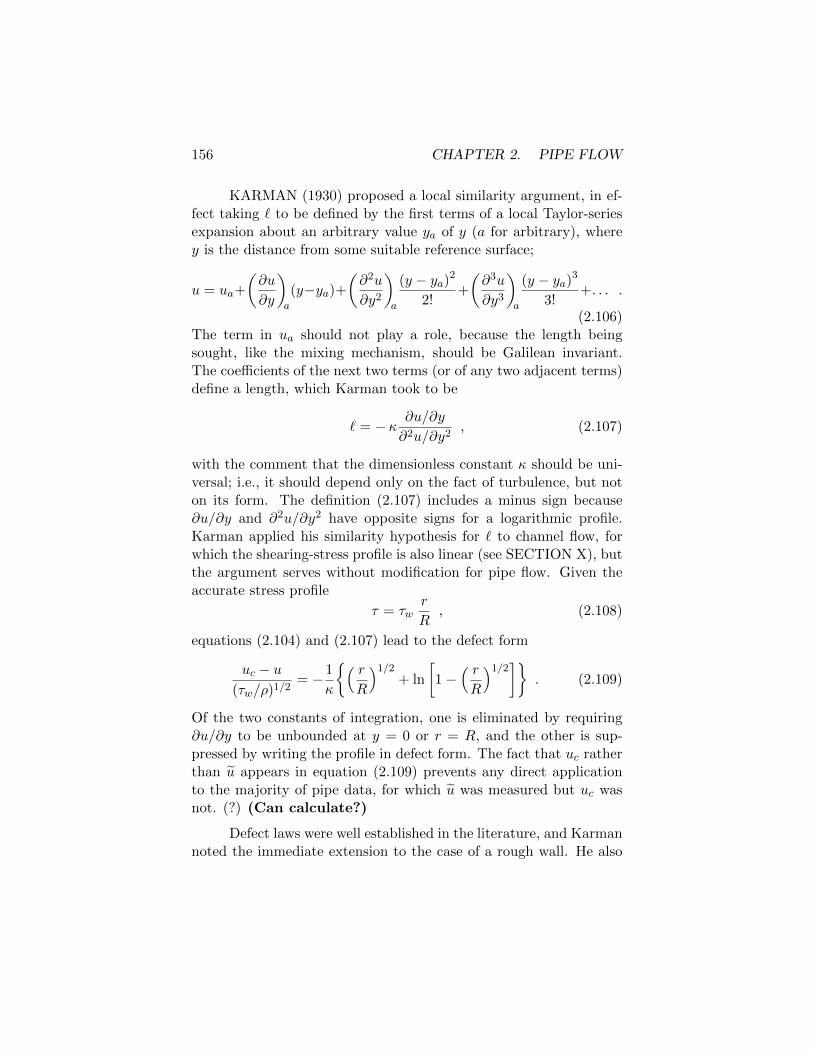
156 CHAPTER 2. PIPE FLOW
KARMAN (1930) proposed a local similarity argument, in ef-fect taking ` to be defined by the first terms of a local Taylor-seriesexpansion about an arbitrary value ya of y (a for arbitrary), wherey is the distance from some suitable reference surface;
u = ua+
(∂u
∂y
)a
(y−ya)+(∂2u
∂y2
)a
(y − ya)2
2!+
(∂3u
∂y3
)a
(y − ya)3
3!+. . . .
(2.106)The term in ua should not play a role, because the length beingsought, like the mixing mechanism, should be Galilean invariant.The coefficients of the next two terms (or of any two adjacent terms)define a length, which Karman took to be
` = −κ ∂u/∂y
∂2u/∂y2, (2.107)
with the comment that the dimensionless constant κ should be uni-versal; i.e., it should depend only on the fact of turbulence, but noton its form. The definition (2.107) includes a minus sign because∂u/∂y and ∂2u/∂y2 have opposite signs for a logarithmic profile.Karman applied his similarity hypothesis for ` to channel flow, forwhich the shearing-stress profile is also linear (see SECTION X), butthe argument serves without modification for pipe flow. Given theaccurate stress profile
τ = τwr
R, (2.108)
equations (2.104) and (2.107) lead to the defect form
uc − u(τw/ρ)1/2
= −1
κ
{( rR
)1/2+ ln
[1−
( rR
)1/2]}
. (2.109)
Of the two constants of integration, one is eliminated by requiring∂u/∂y to be unbounded at y = 0 or r = R, and the other is sup-pressed by writing the profile in defect form. The fact that uc ratherthan u appears in equation (2.109) prevents any direct applicationto the majority of pipe data, for which u was measured but uc wasnot. (?) (Can calculate?)
Defect laws were well established in the literature, and Karmannoted the immediate extension to the case of a rough wall. He also
2.5. SIMILARITY LAWS 157
noted (where?) that in the limit y/R → 0, with τ = τw andy = R− r, his profile formula is reduced to
u
uτ=
1
κln
y
y0, (2.110)
where y0 is a constant of integration. The definition for ` is reducedto (who?)
` = κy , (2.111)
although ` = κy cannot then be distinguished from ` = −κ(∂u/∂y) /(∂2u/∂y2). The notion that ` is proportional to y allows an attractiveinterpretation of ` as the range of a moving fluid element, a rangelimited in one direction by the presence of a wall, and thus varying ina sensible way with the position or perhaps the size of the turbulenteddies.
If in Prandtl’s formula (2.104) the shearing stress is taken asconstant,
τ = τw , (2.112)
then equation (2.110) becomes an exact integral of equation (2.104),with either form for `, when ∂u/∂y is taken to be unbounded fory → 0. (Need sublayer.) The defect form is
uc − u(τw/ρ)1/2
=1
κln(
1− r
R
). (2.113)
It remains to consider the combination of equation (2.111) for ` withequation (2.108) for τ . The corresponding defect form is
uc − u(τw/ρ)1/2
= −1
κ
{2( rR
)1/2+ ln
[1− (r/R)1/2
1 + (r/R)1/2
]}. (2.114)
To recapitulate, two hypotheses (2.107) and (2.111) were pro-posed for `(u, y) and two relationships (2.108) and (2.112) for τ(r).The four combinations are listed in the adjacent TABLE 2.1, togetherwith the associated profile formulas. (Mention values for κ.) Theformula proposed by Darcy is included mainly for completeness. Thefirst profile equation was displayed by KARMAN (1930); the third
158 CHAPTER 2. PIPE FLOW
TABLE 2.1
Mixing-length profiles
mixing shearing defectlength stress profile
equation
` τuc − uuτ
constant τwr
R(2.105)
2
3
R
`
( rR
)3/2
− κ du/dy
d2u/dy2τw
r
R(2.109) − 1
κ
{( rR
)1/2+ ln
[1−
( rR
)1/2]}
− κ du/dy
d2u/dy2τw (2.113) − 1
κln(
1− r
R
)
κy τwr
R(2.114) − 1
κ
{2( rR
)1/2+ ln
[1− (r/R)1/2
1 + (r/R)1/2
]}
κy τw (2.113) − 1
κln(
1− r
R
)
2.5. SIMILARITY LAWS 159
by NIKURADSE (1930); and the second and fourth by KARMAN(1930, 1932), NIKURADSE (1932), and PRANDTL (1932). Appar-ently by 1932 all parties to these developments had accepted the for-mulas (2.110) and (2.113), together with their primitive antecedents,(2.111) and (2.112), as fundamental.
The important parameter (τw/ρ)1/2 was eventually given thename friction velocity (Reibungsgeschwindigkeit) by KARMAN (1932)and denoted by uτ ;
u2τ =
τwρ
. (2.115)
PRANDTL (1927) originally included a factor 1/2 on the left in thedefinition (2.115), in parallel with the definition of dynamic pressure,but later (1932) endorsed the form (2.115) as it stands. One conse-quence is that a factor of 2 survives in the formula Cf = 2τw/ρu
2 =2(uτ/u)2, but a factor of 2 is avoided in several other places, particu-larly in the definition of Newtonian friction at a smooth wall, whichin the limit requires ∂u/∂y = τw/µ = u2
τ/ν ≈ u/y, and therefore
u
uτ=yuτν
. (2.116)
The dimensionless variables u/uτ and especially yuτ/ν both takeon values much larger than unity in the turbulent part of the flow.However, the reference velocity uτ serves another purpose as theproper quantity for making the Reynolds stresses dimensionless, atleast near a wall. Given that these stresses are of comparable mag-nitude and that −ρu′v′ ≈ τ ≈ τw = ρu2
τ , the dimensionless Reynoldsstresses near a wall are necessarily of order unity. Boundary-layerflows that are jet-like or wake-like require different treatment (seeSECTION Y).
At least two serious flaws are contained in equation (2.110).The first is that the formula is a fragment. Within the mixing-lengthmodel, there is no communication with the wall, and no boundarycondition to define the constant y0. (This property is, however, use-ful in dealing with roughness, although a dimensional argument isbetter. Log law implies y0 = 0.49ν/uτ in (2.110)?) For a smoothwall, there is the independent linear limit (2.116). If the complete

160 CHAPTER 2. PIPE FLOW
profile equation is to apply everywhere from the wall to the vicin-ity of the pipe axis, the independent variable must be yuτ/ν, andequation (2.110) should be written
u
uτ=
1
κln
yuτν
+ c (2.117)
outside a transition region first miscalled the laminar sublayer andnow commonly called the viscous sublayer. It is then necessary toexplain why the viscosity is needed to describe the flow in a regionwhere essentially all of the transport is by a turbulent mechanism. Ina dimensional argument first used by KARMAN (1921) in connectionwith the power-law profile (2.131) (see SECTION 2.5.3), the meanvelocity profile is assumed not to depend explicitly on R. It followsthat
u
uτ= f
(yuτν
). (2.118)
This dimensional argument was repeated in this new context byNIKURADSE (1930) in what must have been a hastily prepared pa-per on his experiments, and can probably be attributed to Prandtl.The relationship (2.118), with its linear and logarithmic limits, is nowviewed as fundamental and is commonly referred to as Prandtl’s lawof the wall. The constant κ is known as Karman’s constant. I con-sider these assignments to be fair. Perhaps the best evidence forequation (2.117), if not equation (2.118), is that it fits the experi-mental data. How well it fits, and the best values for the constantsκ and c, will be taken up in SECTION 2.5.7. (How did u makeits way into Nikuradse’s friction law?)
The second and more serious flaw in equation (2.110) is that ithonors the momentum equation in the breach. The shearing stressτ in a pipe is assumed to be constant in a region where it is knownto vary substantially. Nevertheless, the logarithmic formula is foundto fit the data. More extreme cases having the same property, par-ticularly the sink-flow boundary layer and the wall jet, are cited inSECTIONS X and Y below. In any case, the logarithmic profile hasno certain connection with the laws of mechanics as these laws arepresently understood for turbulent flow.

2.5. SIMILARITY LAWS 161
To make this same point in another way for the case of pipeflow, the three distinct formulas in the table are plotted in defect formin FIGURE X, 12 together with an experimental profile from the workof LAUFER (1953) that uses an approximate value Ruτ/ν = xxxx.The best agreement is seen for the logarithmic profile based on thecondition τ = τw. This fact may or may not justify the concept of aconstant-stress layer (amplify). The discrepancy between formulaand data is larger when the momentum equation and the exact for-mula τ = τwr/R are used, rather than the approximation τ = τw.The discrepancy near the center of the pipe is real (see SECTION X),so that this observation may not be central. However, it illustratesa problem common to many mixing-length methods for modelingturbulent flow, in that attempts to increase the level of rigor or therange of application often lead to a worse result.
Thus the provenance of the logarithmic law of the wall. Themixing length is an exasperating concept. It survives because itpoints easily to a logarithmic dependence of the mean velocity onthe distance from a wall. There is no doubt that this observationwas a huge step forward at the time. A cynic might say that it res-cued engineers from the tyranny of log-log paper and delivered themto the greater tyranny of semi-log paper. A romantic would say thatit led to important real advances, because the whole episode of themixing-length analogy raised the consciousness of engineers and sci-entists by revealing an intrinsic order in the subject and by suggestingthat there might be other equally simple phenomenological relation-ships waiting to be discovered. There is still no better formalism fororganizing the effects of mass transfer at a wall, of lateral curvature,or of compressibility. Nevertheless, the ideas that could be classifiedas insight in 1930 must by now be reclassified as peripheral vision,in the terminology of the introduction.
My position is that the mixing-length model does not explainthe logarithmic profile. Neither does either of two alternative argu-ments (section x, Millikan, and section y, singular perturbation), orany other argument known to me. (Work on extremum principle.)For the present, I accept the logarithmic profile as an empirical fact,
12This figure appears never to have been created.
162 CHAPTER 2. PIPE FLOW
and will turn in SECTION 2.5.7 to the practical question of deter-mining values for the constants κ and c in equation (2.117). Somevaluable inferences from the law of the wall in the more general form(2.118) will be presented in section x of the chapter on boundarylayers.
2.5.2 The Izakson-Millikan argument
An important contribution to the subject was made by IZAKSON(1937) and repeated by MILLIKAN (1938). The logarithmic formula(2.117) was originally proposed to describe nearly the whole flow in apipe, for which departures from the formula outside the sublayer areexperimentally small and were not emphasized at the time. Thesedepartures are more conspicuous in a boundary layer, and are dis-cussed at length in SECTION X. For the moment, it is enough tonote that equation (2.117) becomes at the center of the pipe
ucuτ
=1
κln
Ruτν
+ c , (2.119)
where uc is the mean velocity on the axis and R is the pipe radius.The viscosity can be eliminated by subtraction to obtain a formulafirst proposed by Karman (ref),
uc − uuτ
= −1
κln
y
R. (2.120)
This formula is experimentally incomplete, and needs another term,now commonly called the wake component, that also depends onlyon y/R. Thus, more generally, equation (2.117) can be written, inMillikan’s notation,
u
uτ=
1
κln
yuτν
+ c+ h( yR
), (2.121)
from which
uc − uuτ
= −1
κln
y
R+ h(1)− h
( yR
)= F
( yR
). (2.122)
2.5. SIMILARITY LAWS 163
This expression is usually called Karman’s velocity-defect law. It isat least plausible that the mean-velocity defect should depend onlyon the stress level τw and not on µ.
The Izakson-Millikan argument assumes that there is a finiteregion where both equation (2.118) and equation (2.122) are valid.In this region,
∂u
∂y=u2τ
νf ′ = −uτ
RF ′ , (2.123)
or, in an obvious notation,
zf ′(z) = −ζF ′(ζ) . (2.124)
Since the Reynolds number Ruτ/ν, which is the ratio z/ζ of the twoarguments, is arbitrary, the two sides of equation (2.124) must beseparately constant. Call this constant 1/κ. Integrate to obtain
f(z) =1
κln z + constant , (2.125)
or, in physical variables,
u
uτ=
1
κln
yuτν
+ c . (2.126)
Thus the mean-velocity profile in the common region is logarithmic.The terms of the derivation just given imply that the constant κ isindependent of Reynolds number. (Note fashions, timing, andmany examples of papers being ignored.) This argument waspublished in 1937-1938, when the major activity in the subject wasdevelopment of the mixing-length model. It languished for more than15 years until Hans Liepmann called it to my attention about 1950when I was searching for an alternative argument for the logarithmicbehavior of the profile in terms of similarity laws rather than mixing-length ideas.
2.5.3 The power-law profile
A proper chronology requires a short summary here of the power-law velocity profile, which was first proposed publicly by KARMAN
164 CHAPTER 2. PIPE FLOW
(1921) in a powerful paper that is notable for other reasons; namelythat it contains the boundary-layer approximation as a formal innerlimit of the Navier-Stokes equations for small ν, as well as the essenceof the singular-perturbation method, including inner and outer ex-pansions, the matching condition, and the composite expansion. Italso introduces the momentum-integral equation for the boundarylayer, an equation that is exploited for the case of laminar flow in thefollowing paper by POHLHAUSEN (1921). These practical develop-ments finally forced the acceptance of the boundary-layer concept,with all of its associated advances, by the rest of the world fluid-mechanics community. In fact, Karman discussed pipe flow and thepower-law profile primarily as a device to model the boundary layer.He derived a formula for flat-plate friction that agreed reasonablywell with early towing-tank measurements of total drag. Note thatthere were, for practical purposes, no profile measurements in bound-ary layers in 1921, and precious few profile measurements in classicalpipe flow (check work on roughness).
Part of the reason for this was lack of proper instrumentationas well as the poor quality of existing wind tunnels, as made evidentby a paper by Prandtl (1924; check). (Did the British have goodtunnels? See Prandtl and Tietjens.) This lack probably inspiredwork in 1924 by van der Hegge Zijnen under Burgers, taken up insection x. It probably also inspired in part the profile measurementsin smooth pipes by Nikuradse (1930, 1932), following Nikuradse’sthesis on secondary flow in non-circular pipes.
Karman based the relevant section of his 1921 paper on theobservation by BLASIUS (1913) that the friction coefficient for tur-bulent pipe flow at Reynolds numbers from 5,000 to 100,000 couldbe well fitted by a power law,
Cf = constant Re−1/4 . (2.127)
In dimensional form this is
τw = ρu2τ = constant ρu7/4(ν/D)1/4 . (2.128)
This relationship emerges from a pursuit of straight lines on log-log paper. Karman noted that the systematic dependence of Cf
2.5. SIMILARITY LAWS 165
on Re implied a systematic variation of the mean-velocity profile.He assumed that the profile in some region, eventually taken to bethe whole of a pipe flow except for a thin layer very near the wall,depended on a restricted set of variables,
u = u(ρ, µ, τw, y) (2.129)
where the radius R is omitted and y = R − r is measured from thewall toward the axis. The pressure gradient dp/dx need not be con-sidered because it is interchangeable with τw according to equation(2.11). (What about D?) The mean velocity u need not be con-sidered because it is an integral of the profile u according to equation(2.15). Equation (2.129) in dimensionless form implies the relation-ship known as the law of the wall (see SECTION 2.5.4),
u
uτ= g(yuτν
). (2.130)
In the present context, this relationship is taken to be a power law,
u
uτ= B
(yuτν
)n(2.131)
Then
u = Bun+1τ (y/ν)n (2.132)
and, if the formula extends to the axis,
uc = Bun+1τ (R/ν)n (2.133)
so that u/uc depends only on y/R, independent of Reynolds number.
Finally, the mean velocity u is obtained by putting the profile(2.132) in the definition (2.15),
u =2B
(n+ 1)(n+ 2)un+1τ (R/ν)n (2.134)
from which (need constants)
ρuτ2 = constant ρu2/(n+1)(ν/D)2n/(n+1) . (2.135)
166 CHAPTER 2. PIPE FLOW
Comparison with equation (2.128) yields immediately n = 1/7 fromeither exponent. This is a local and empirical result that applies atbest only in a restricted range of Reynolds numbers. It has sincebeen overtaken by events, as will be explained in the next section.Nevertheless, it may occasionally be useful for making rapid esti-mates.
KARMAN (1921, 1930) noted that Prandtl had already ob-tained these results in 1920 by a somewhat different argument, andPRANDTL eventually published his own version some years later(1927, III Lieferung). The main difference is the means used to passfrom the mean velocity u, used in the friction equation, to the cen-terline velocity uc, used in the profile equation. (check).
2.5.4 The dimensional argument
The preceding section moves the empirical content of the mean-velocity profile in turbulent pipe flow from the mixing length to thesimilarity laws (2.118) and (2.122). These laws can be rationalized,although not explained, by a dimensional argument. First, supposethat the velocity as observed from the wall depends on the parame-ters according to (this needs work)
u = f(y, ρ, ν, τw, R, uc) , (2.136)
where the mean velocity u is not displayed because it is implicit whenf is known, and dp/dx is not displayed because it is determined fora pipe by τw and R (redundant). Suppose that u is found not todepend on R or uc. (Mention atmosphere; no δ or uc.) Theonly dimensionally correct form for u(y) is then equation (2.118).Suppose further that the velocity observed from the pipe center,
uc − u = F (y, ρ, ν, τw, R) , (2.137)
is found not to depend on ν. The only dimensionally correct formfor [uc − u(y)] is then equation (2.122), and the Izakson-Millikanargument follows. The weakness of this argument becomes clear onlywhen there is another parameter with the dimensions of a velocity or
2.5. SIMILARITY LAWS 167
a length, such as a suction or blowing velocity vw, or a roughness scalek at the wall, or a body diameter D in the case of boundary-layerflow on the outside of a cylindrical body. The nature and role of thenew dimensionless parameter have to be determined in each case bya fresh empirical assault on the problem. Effects of compressibilityand effects of suction or blowing at the wall, in particular, are stillbest described in terms of the mixing-length model (van Driest), andare therefore not under control.
(Straighten out the question of an analogy with Kolmogorov’sargument for the spectrum; see the introduction. See Narasimha.Mention separation of variables and singular perturbations.) (Intro-duce u+, y+ notation.) 13
2.5.5 Interpolation formulas for the sublayer
The linear and logarithmic versions of the law of the wall, equations(2.116) and (2.117), intersect at a point near u+ = y+ = 11, depend-ing on the values chosen for the constants κ and c. (Another inter-section, at a free outer boundary of flow near a wall, is discussed inSECTION X of Chapter 4 on boundary layers.) For some purposes,the idea of a sharp intersection can be valuable, because it serves asa primitive definition of sublayer scale. For example, DONALDSON(1952) used a model with a linear sublayer and a power-law outerprofile to argue that the main effect of compressibility in boundary-layer flow is to increase the relative thickness of the sublayer. For thepresent purpose, what matters is that the discontinuity in ∂u/∂y atthe linear-logarithmic intersection implies a corresponding disconti-nuity in both components of the total shearing stress. Let this totalstress be taken as constant; thus
τ = µ∂u
∂y− ρu′v′ = τw , (2.138)
or, in dimensionless wall units,
τ
τw=
du+
dy+− u′v′
uτ 2= 1 . (2.139)
13This notation is explained in section 2.5.6
168 CHAPTER 2. PIPE FLOW
Equation (2.139) is exact for plane Couette flow (SECTION X) andis otherwise an approximation in and near the sublayer for largeReynolds numbers. This equation is the point of departure for themodeling that follows. The discussion will neglect any effects of lat-eral curvature, pressure gradient, or low Reynolds number on the lawof the wall, since it is not certain that these effects are experimentallydetectable (see SECTION X).
When the law of the wall is expressed in Prandtl’s form, u+ =f(y+), the implication is that the sublayer intersection has beenrounded off by recourse to some formula based on experimental data.A corresponding rounding is needed for the laminar and turbulentshearing stresses in equation (2.138). These stresses have a constantsum, with the laminar stress µ∂u/∂y rapidly decreasing and the tur-bulent stress −ρu′v′ rapidly increasing in a close neighborhood of thewall. In fact, it is the region in which the exchange of mechanismstakes place that is properly called the sublayer. Because the laminarshearing stress is known if the function u+ = f(y+) is known, the keyto the problem lies in the turbulent shearing stress, and specificallyin the fact that the quantity u′v′ behaves like y3 very near the wall.I will argue this property in detail, I hope persuasively, in SECTION
X. For the present, it is sufficient to stipulate that (u′u′)1/2
behaves
like y and that (v′v′)1/2
behaves like y2, according to the continu-ity equation. The result u′v′ ∼ y3 then follows, as was first argued,somewhat tentatively, by REICHARDT (1951).
The need for an interpolation formula is most apparent in prob-lems of heat transfer, especially at high Prandtl numbers (see SEC-TION X). MURPHREE (1932) and KARMAN (1939) introduced aprimitive buffer layer for such problems (look up Murphree, others;Reynolds’ analogy). Since then, more than 50 papers have been pub-lished on the interpolation problem. The literature up to about 1965is thoroughly surveyed in the thesis by COANTIC (1966), and themore recent literature can be traced through papers by LEWKOW-ICZ (1982) and by NARAYANA and RAMANA (1988). Many ofthese papers patch various sublayer profiles to the logarithmic pro-file. A few papers provide a single continuous analytic formula forthe entire region; i.e., an explicit formula u+ = f(y+), or its inverse.
2.5. SIMILARITY LAWS 169
I will discuss three such formulas and recommend one of them.
Van Driest. A formula based on the mixing-length model andthe approximation τ = τw was proposed by VAN DRIEST (1956).Van Driest explains his approach by writing
− u′v′ = r(u′u′)1/2
(v′v′)1/2
, (2.140)
where r is a dimensionless correlation coefficient that is known exper-imentally to be the most nearly universal number in all of turbulence,having a value near 0.4 or 0.5 in large regions of many different shearflows. (Give phase argument?) The universality of r can be inter-preted as evidence that various active Reynolds stresses tend to beproportional to each other in fully developed turbulent flow, or moreconstructively as a statement about a common phase relationship
between the fluctuations u′ and v′. Van Driest writes (u′u′)1/2
and
(v′v′)1/2
as `′ ∂u/∂y and `′′ ∂u/∂y. The two mixing lengths `′ and`′′ and the coefficient r are then combined as `2 to obtain Prandtl’sequation,
− ρu′v′ = ρ`2(∂u
∂y
)2
. (2.141)
To model the effect of damping by the wall, Van Driest invokesthe STOKES solution (1851) for a wall oscillating harmonically inits own plane in a stationary viscous fluid. For this flow, the fluc-tuations away from the wall are exponentially damped, like e−y/L,where the damping scale L = (2ν/ω)1/2 depends on frequency. VanDriest assumes that for a fixed wall and an oscillating fluid the corre-sponding damping factor is (1−e−y/λ), although the solution derivedby LAMB (1932, p. 622) behaves differently. This assumed dampingfactor is applied twice, together with ` = κy, to obtain
− ρu′v′ = ρκ2y2(
1− e−y/λ)2(∂u
∂y
)2
. (2.142)
Unfortunately, this equation has u′v′ behaving like y4 near the wall.CHAPMAN and KUHN (1986) argue that the correct behavior canbe obtained if the damping factor is associated with u′u′, as suggested
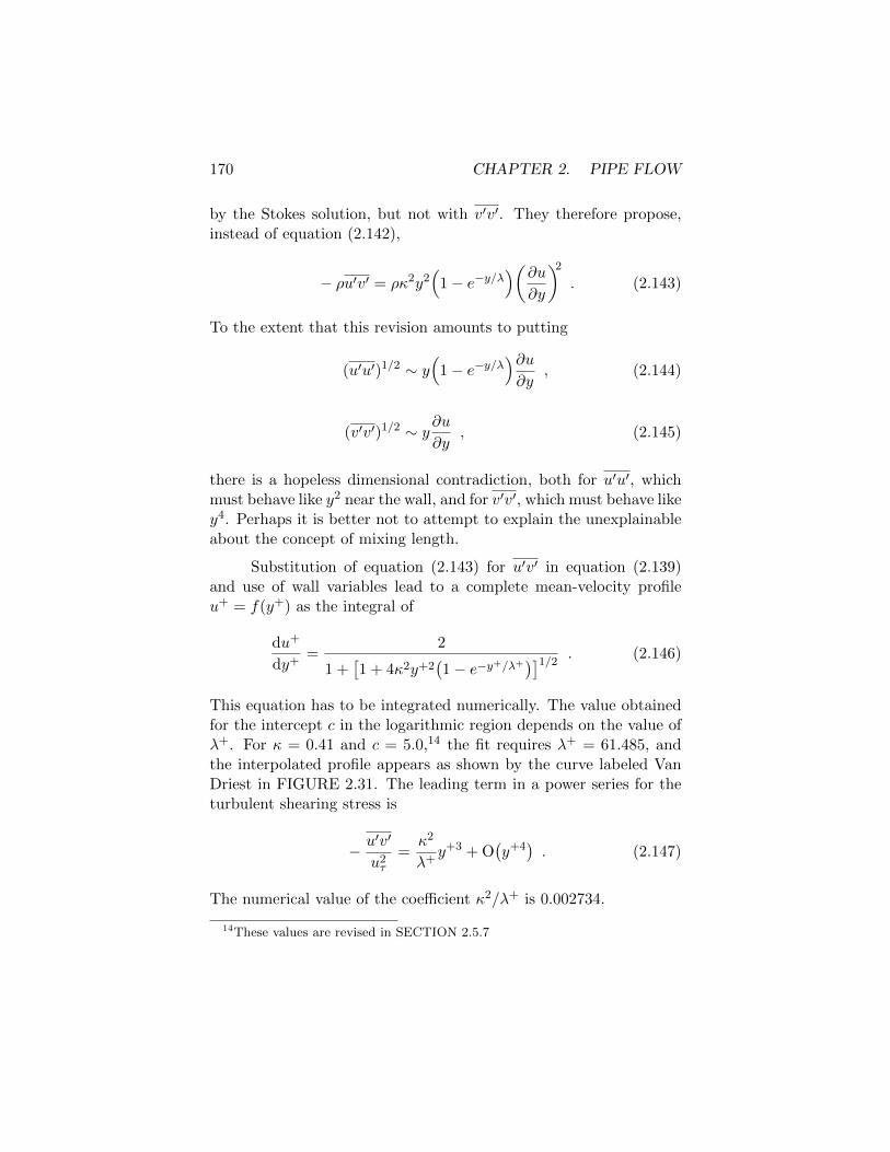
170 CHAPTER 2. PIPE FLOW
by the Stokes solution, but not with v′v′. They therefore propose,instead of equation (2.142),
− ρu′v′ = ρκ2y2(
1− e−y/λ)(∂u
∂y
)2
. (2.143)
To the extent that this revision amounts to putting
(u′u′)1/2 ∼ y(
1− e−y/λ)∂u∂y
, (2.144)
(v′v′)1/2 ∼ y∂u∂y
, (2.145)
there is a hopeless dimensional contradiction, both for u′u′, whichmust behave like y2 near the wall, and for v′v′, which must behave likey4. Perhaps it is better not to attempt to explain the unexplainableabout the concept of mixing length.
Substitution of equation (2.143) for u′v′ in equation (2.139)and use of wall variables lead to a complete mean-velocity profileu+ = f(y+) as the integral of
du+
dy+=
2
1 +[1 + 4κ2y+2
(1− e−y+/λ+
)]1/2 . (2.146)
This equation has to be integrated numerically. The value obtainedfor the intercept c in the logarithmic region depends on the value ofλ+. For κ = 0.41 and c = 5.0,14 the fit requires λ+ = 61.485, andthe interpolated profile appears as shown by the curve labeled VanDriest in FIGURE 2.31. The leading term in a power series for theturbulent shearing stress is
− u′v′
u2τ
=κ2
λ+y+3 + O
(y+4). (2.147)
The numerical value of the coefficient κ2/λ+ is 0.002734.
14These values are revised in SECTION 2.5.7

2.5. SIMILARITY LAWS 171
100 101 102 103 104
0
10
20
30
0
0
0
0
Musker (1979)Spalding (1961)Van Driest (1956)
u+
y+
Figure 2.31: Three interpolation formulas for the
transition region between the linear and logarithmic
forms of the law of the wall. Note the displaced
scales. The top display is a superposition of the other
three. I recommend the formula proposed by Musker.
172 CHAPTER 2. PIPE FLOW
Equation (2.147) defines a family of profiles, with λ+ or c asparameter. Check these for suitability for showing effects of rough-ness or polymers. Van Driest has a more general scheme that doesnot inspire confidence. What value of ω goes with the specified λ?
Spalding. A quite different proposal was put forward bySPALDING (1961) and independently by KLEINSTEIN (1967). Thedifficulty that u(y) does not have a power-series expansion valid intothe log region can be avoided if y(u) is examined instead. The loga-rithmic law,
u+ =1
κln y+ + c , (2.148)
has the inversey+ = e−κceκu
+. (2.149)
This expression does have a power-series expansion about u+ = 0,namely
y+ = e−κc[1 + (κu+) +
(κu+)2
2+
(κu+)3
6+
(κu+)4
24+
(κu+)5
120+ · · ·
],
(2.150)with an infinite radius of convergence. If a valid expansion is to beginwith a term in u+ and continue with a term in (u+)4, on the premisethat u+ begins with a term in y+ and continues with a term in (y+)4
(see SECTION X), it is sufficient to cancel the first four terms of theseries and append a term in u+; thus
y+ = u+ + e−κc
[eκu
+ − 1− (κu+)− (κu+)2
2− (κu+)3
6
]. (2.151)
This manufactured interpolation formula incorporates the two limit-ing forms (2.116) and (2.117) of the wall law, as shown by the curvelabeled Spalding in FIGURE 2.31. However, convergence to the log-arithm is relatively slow, and there are no disposable parameters.The leading term in an expansion of u′v′ is found to be
− u′v′
u2τ
=e−κcκ4
6y+3 + O(y+4) . (2.152)
For κ = 0.41 and c = 5.0, the coefficient of y+3has the numerical
value 0.000606.
2.5. SIMILARITY LAWS 173
Musker. It remains to put in evidence MUSKER’s proposal(1979), which emerges from the concept of eddy viscosity. Withequation (2.138) in mind, define an eddy viscosity µt by
− ρu′v′ = µt∂u
∂y(2.153)
and a kinematic eddy viscosity νt = µt/ρ by (cite Boussinesq)
− u′v′
u2τ
=νtν
du+
dy+. (2.154)
Equation (2.139) can now be written
τ
τw=(
1 +νtν
) du+
dy+= 1 . (2.155)
Very close to the wall, where u′v′ behaves like y3, the left side ofequation (2.154) is O(y+3), and du+/dy+ is O(1). Consequently, put
νtν
= sy+3 forνtν� 1 , (2.156)
where s (for shearing stress) is an empirical constant.
(Note that equation (??) in section x is an exact consequenceof the law of the wall in the form u+ = f(y+). By coincidence, theleading term in an expansion of the integral in this equation is alsoa term in y3. However, this term is normally orders of magnitudesmaller than the estimate (2.156) because of the factor λ+ in thedenominator.) (λ twice).
In the logarithmic region, where du+/dy+ = 1/κy+, take theshearing stress to be constant and put
νtν
= κy+ forνtν� 1 . (2.157)
Musker’s proposal is to satisfy the two limiting conditions (2.156)and (2.157) on νt/ν simultaneously by using what I call the lensformula,
1
νt/ν=
1
sy+3 +1
κy+=κy+ + sy+3
sκy+4. (2.158)

174 CHAPTER 2. PIPE FLOW
Consequently, from equation (2.155),
du+
dy+=
y+2
κ+
1
s
y+3 +y+2
κ+
1
s
. (2.159)
This equation can be expanded in a power series about y+ = 0 toobtain
− u′v′
u2τ
= 1− du+
dy+= sy+3 − s2
κy+5 + O
(y+6). (2.160)
Term-by-term integration gives
u+ = y+ − s
4y+4 +
s2
6κy+6 + O
(y+7). (2.161)
To lowest order, the turbulent shearing stress is half of the total wheny+ is about 7.7, in keeping with traditional ideas about the scale ofthe sublayer. (Cite Spalart’s calculations for the boundary layer atconstant pressure, which indicate that the first two terms for u′v′
are terms in y3 and y5. Coincidence? Mention consequences for fullexpansion in chapter 7.)
Musker’s analytical integration of equation (2.159) is worthstudy. Let the denominator be expressed as (y+−a)(y+−b)(y+−c).One of the three roots is real and negative, and the other two arecomplex conjugates, as shown in FIGURE 2.32. Write
a < 0, b = α+ iβ, c = α− iβ . (2.162)
The three roots satisfy the identities
a+ b+ c = a+ 2α = −1
κ, (2.163)
ab+ ac+ bc = 2aα+R2 = 0 , (2.164)
abc = aR2 = −1
s, (2.165)
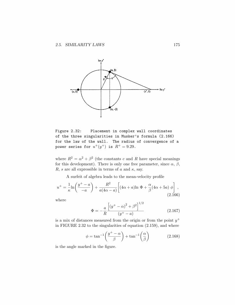
2.5. SIMILARITY LAWS 175
Figure 2.32: Placement in complex wall coordinates
of the three singularities in Musker’s formula (2.166)
for the law of the wall. The radius of convergence of a
power series for u+(y+) is R+ = 9.29.
where R2 = α2 + β2 (the constants c and R have special meaningsfor this development). There is only one free parameter, since α, β,R, s are all expressible in terms of a and κ, say.
A surfeit of algebra leads to the mean-velocity profile
u+ =1
κln
(y+ − a−a
)+
R2
a(4α− a)
[(4α+ a)ln Φ +
α
β(4α+ 5a) φ
],
(2.166)where
Φ = − aR
[(y+ − α)
2+ β2
]1/2
(y+ − a)(2.167)
is a mix of distances measured from the origin or from the point y+
in FIGURE 2.32 to the singularities of equation (2.159), and where
φ = tan−1
(y+ − αβ
)+ tan−1
(α
β
)(2.168)
is the angle marked in the figure.
176 CHAPTER 2. PIPE FLOW
The boundary condition u+ = 0 at y+ = 0 is evidently satis-fied by equation (2.166). Passage in either direction to verify thatthis equation is the integral of equation (2.159) is aided by the iden-tities (2.163)–(2.165). Because equations (2.163) and (2.164) implyR2/a2 < 1, the complex roots determine the radius of convergenceR of the power series expansions (2.160) and (2.161).
For sufficiently large values of y+, the profile equation takesthe form
u+ =1
κln y+ + c , (2.169)
where c is now the constant of integration first defined in equation(2.117);
c = −1
κln(−a) +
R2
a(4α− a)
{(4α+ a)ln
(− aR
)+α
β(4α+ 5a)[
π
2+ tan−1
(α
β
)]}. (2.170)
Since c and s can both be expressed parametrically in terms of a,they are uniquely related to each other. Given κ = 0.41, the valuesthat correspond to c = 5.015 are a = −10.593, α = 4.077, β = 8.352,R = 9.294, and s = 0.001093. These constants in equation (2.166)produce the lowest labeled curve in FIGURE 2.31.
Musker’s profile slightly overshoots the log profile, by a max-imum of about 0.02 in u+ near y+ = 150. This minor defect couldprobably be removed by slightly increasing the coefficient of the mid-dle term in the denominator of (2.159), to decrease the derivativedu+/dy+ locally without disturbing the two limiting conditions, butI prefer to rest my case.
Although the profile equation (2.166) is untidy, Musker’s inter-polation scheme works so well that its use amounts to making a neces-sity out of virtue. First, the leading terms in the power series for u′v′
agree with the leading terms extracted from SPALART’S numericalresults (1988) for the turbulent boundary layer at constant pressure,as shown in FIGURE X.16 (Check this. Get channel numbers
15Values of κ and c are revised in SECTION 2.5.716This figure has not been found.
2.5. SIMILARITY LAWS 177
from Moin.) Second, there is an encouraging resemblance betweenthe pattern of singularities in FIGURE 2.32 and the correspondingpattern for the Blasius boundary layer (see SECTION X), thus pro-viding another point of contact in the power-series approach to bothlaminar and turbulent regimes of flow near a wall. Finally, Musker’sscheme, although it has only one disposable constant, is capable ofgenerating a plausible family of profiles for fixed κ and arbitrary c,and I will use it for this purpose when I take up some effects of surfaceroughness and long-chain polymers in SECTIONS 2.6 and 2.7.
2.5.6 Fully developed flow
One test for fully developed pipe flow can be based on the propertiesof the mean velocity profile, provided that an accurate analyticaldescription of the profile is available. Such a description is given inpart by the empirical formula
u
uτ= f
(yuτν
)+
Π
κw( yR
), (2.171)
where uτ and Π are parameters. The function f outside the sublayeris a logarithm, and w is an antisymmetric function that is adequatelyrepresented by sin2 (πy/2R). The distance y is measured from thewall toward the axis and beyond.
One defect in the formula (2.171) is the presence of a corner, ordiscontinuity in slope, on the pipe axis. The equivalent defect at theedge of a boundary layer is discussed at length in SECTION 4.9.3below. In the present section, the need is to develop a quantitativemeasure of the degree of rounding of the experimental velocity profilenear the pipe axis, thus creating a new and sensitive criterion forjudging the approach to full developments. The notation refers topipe flow, but the physical meaning may be clearer if the calculationsare associated with channel flow.
The discontinuity in slope appears when the wall law outsidethe sublayer is written as
u
uτ=
1
κln
yuτν
+ c (2.172)

178 CHAPTER 2. PIPE FLOW
1:0
u+
-10115
20
25
r
R
0.20.5
1:0
n = 0:1
Figure 2.33: Use of the single-parameter equations
(2.176) and (2.180) to round the logarithmic
mean-velocity profile near the pipe axis for the case
R+ = Ruτ/ν = 2000.
and this law is assumed to hold to the pipe axis at y = R. Recallthe analytical device that I called the lens formula in the previoussection. (check) The objective there was to interpolate betweenthe linear and logarithmic parts of the mean-velocity profile in thesublayer. The same device will be used here. The notation is shownin FIGURE 2.33. For the left half of the figure, the law of the wallhas the form (2.172). For the right half of the figure, write
u
uτ=
1
κln
(2R− y)uτν
+ c , (2.173)
where y in both formulas is measured from the left wall. For brevity,introduce the + notation, with u+ = u/uτ , y+ = yuτ/ν, and R+ =Ruτ/ν. Close to the left wall in FIGURE 2.33, define a new variable
2.5. SIMILARITY LAWS 179
Y + by the identity
Y + = y+ . (2.174)
Close to the right wall, define the same variable by
Y + = 2R+ − y+ , (2.175)
so that the single formula
u+ =1
κln Y + + c (2.176)
applies close to both walls. Near the axis, the two definitions for Y +
can be joined smoothly with the aid of the lens formula,
1
(Y +)1/n=
1
(y+)1/n+
1
(2R+ − y+)1/n; (2.177)
or
Y + =
[(2R+ − y+)
1/n(y+)1/n
(2R+ − y+)1/n + (y+)1/n
]n, (2.178)
where the parameter n determines the amount of rounding near theaxis. Finally, replace the distance y, measured from the left wall, bythe distance r, measured from the axis of the pipe;
y+ = R+ − r+ . (2.179)
Given that y+ is always positive, the radius r+ must be interpreted aspositive (negative) in the left (right) half of FIGURE 2.33. Equation(2.178) becomes
Y + =
[ (R+2 − r+2
)1/n(R+ + r+)1/n + (R+ − r+)1/n
]n. (2.180)
This form shows explicitly the desired symmetry about the pipe axis,with Y +(r+) = Y +(−r+) everywhere. Some typical rounded profilesdefined by equations (2.176) and (2.180) are shown in the figure forseveral values of n. On the axis, where r+ = 0, Y + = R+/2n. If amore physical interpretation of the parameter n is wanted, it can be

180 CHAPTER 2. PIPE FLOW
had by calculating the radius of curvature of the function u+ (r+) atr+ = 0, most simply by way of power-series expansions. (Do this.)
(Two paragraphs out of order.) A few remarks are inorder about the conceptual nature of the variables just considered.The quantities called the Reynolds stresses are part of the Reynolds-averaged momentum equations, and so must answer to the laws ofmechanics. My view is that at least the Reynolds shearing stresscan be intrepreted as a real physical variable. Within the boundary-layer approximation, a numerical value can be assigned to −ρu′v′in at least two ways. The first defines this quantity as an apparentforce required to balance other forces and accelerations that can beevaluated independently. The second measures the fluctuations u′
and v′ and the mean value of their product. The two quantities sodetermined will be compared for a variety of flows in different sectionsof this monograph. If the two values do not agree, the difference isordinarily blamed on failure of the boundary-layer approximationor on experimental error. This view may survive the assumptionτ = τw, although the laws of mechanics are then abandoned, asalready pointed out in SECTION X.
The mixing length and the eddy viscosity are conceptually dif-ferent from the Reynolds stresses and from each other. A numericalvalue can be asssigned to ` or to µt in only one way, through the def-inition (2.141), in the case of `, or the definition (2.153), in the caseof µt. These definitions lie outside the laws of mechanics, being partof turbulence modeling. They are inventions that are intended tosupply an additional equation to be used with momentum equationslike (2.1), but in practice are often used alone. The eddy viscosity isthe kinder concept, being a direct surrogate for the velocity field.
My plan is to fit turbulent profiles and determine Π and n.Plot Π and n vs R+. Plot Π vs n. Look for evidence of lack ofdevelopment or lack of symmetry.
Suitable profiles are in papers by
COSTRELL processFOWLES
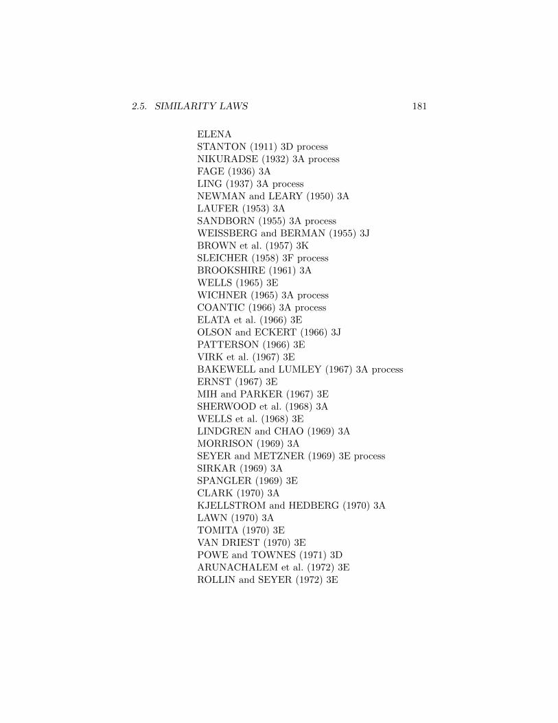
2.5. SIMILARITY LAWS 181
ELENASTANTON (1911) 3D processNIKURADSE (1932) 3A processFAGE (1936) 3ALING (1937) 3A processNEWMAN and LEARY (1950) 3ALAUFER (1953) 3ASANDBORN (1955) 3A processWEISSBERG and BERMAN (1955) 3JBROWN et al. (1957) 3KSLEICHER (1958) 3F processBROOKSHIRE (1961) 3AWELLS (1965) 3EWICHNER (1965) 3A processCOANTIC (1966) 3A processELATA et al. (1966) 3EOLSON and ECKERT (1966) 3JPATTERSON (1966) 3EVIRK et al. (1967) 3EBAKEWELL and LUMLEY (1967) 3A processERNST (1967) 3EMIH and PARKER (1967) 3ESHERWOOD et al. (1968) 3AWELLS et al. (1968) 3ELINDGREN and CHAO (1969) 3AMORRISON (1969) 3ASEYER and METZNER (1969) 3E processSIRKAR (1969) 3ASPANGLER (1969) 3ECLARK (1970) 3AKJELLSTROM and HEDBERG (1970) 3ALAWN (1970) 3ATOMITA (1970) 3EVAN DRIEST (1970) 3EPOWE and TOWNES (1971) 3DARUNACHALEM et al. (1972) 3EROLLIN and SEYER (1972) 3E
182 CHAPTER 2. PIPE FLOW
TOWNES et al. (1972) 3DCARPENTER (1973) 3DLU et al. (1973) 3HBERTELRUD (1974) 3A processCHEN and ROBERTSON (1974) 3DDURST and KELLER (1974) 3EPATEL (1974) 3A processSCRIVENER (1974) 3EAQUINO and LAMONTAGNE (1975) 3EPERRY and ABELL (1975) 3A processSABOT and COMTE-BELLOT (1976) 3AMIZUSHINA and USUI (1977) 3EHISHIDA and NAGANO (1979) 3AKUBO (1979) 3ESCHILDKNECHT et al. (1979) 3JRAMAPRIAN and TU (1980) 3HHASSAN (1980) 3ADURST et al. (1981) 3ELANGEHEINEKEN (1981) 3ATU and RAMAPRIAN (1983) 3HBEWERSDORFF (1985) 3EBULLOCK et al. (1990) 3D
2.5.7 Karman’s constants κ and c
NOTE: The first four paragraphs in this section were includedin the draft of this chapter. A separate file dated 1 April 1999 withnew conclusions of the author on the same topic has been added atthe label ’Revision of values.’ –K. Coles
The values of Karman’s constants κ and c in the logarith-mic profile are usually thought to be determined from Nikuradse’ssmooth pipe data, whether or not the wake component is clearlyrecognized. The universal parameter κ originates in the heuristicdefinition du/dy = uτ/κy in Prandtl’s equation (2.104) with ` = κyand τ = τw, although sometimes κ is inferred after one or more stagesof manipulation. Numerous other measurements of pipe profiles have
2.5. SIMILARITY LAWS 183
been made, and should also be considered as evidence. A preliminarystep is to ensure from other evidence that the flow is fully developed.A suitable test is to obtain the strength of the wake component andlook for a universal behavior. I take figure x as the best evidence forthe value of these constants.
A second major source of systematic data on the mean-velocityprofile in a smooth pipe at large Reynolds numbers is the thesis byLING (1939), who studied under Schoder at Cornell University. Thisthesis has some anomalous properties. The experimental apparatus isnot described in convincing detail. There is no attempt to comparethe results with the results of other experimenters. Finally, thereis little evidence in some sections of the thesis that the work wasproperly supervised. It is not possible sixty years later to accountfor these anomalies, or even to determine why the research was doneat all. Nevertheless, I am willing to accept Ling’s results, and theyare shown in figure x.
(Select possible experiments from DATA3A. Evaluate two con-stants by plotting the wall law in the range y+ > 50 (or 100) andy/R < 0.25, to isolate the logarithmic region. Look at uc/u to findpoor data. Look at uc/uτ or friction coefficient for the same purpose.Can anything be done with Burke’s data? Emphasize that κ and care defined in terms of the mean-velocity profile, equation (2.117).Collect data; there are at least 50 sources. (Data are available forNikuradse, Stanton, Bertelrud, Ramaprian and Tu, Deissler, Wich-ner, Brookshire, Coantic, Ling, Patel, Hettler, Fowles, Sirkar, Shaverand Merrill, Bogue and Metzner, Hershey, Virk et al, Seyer andMetzner, Wang. Data are needed for Chen and Robertson, Laufer,Langeheineken, Hishida and Nagano, Hassan, Morrison, Fage, Clark,Bakewell and Lumley, Sherwood et al, Durst et al, Durst and Keller,Patterson et al, Wells, Perry and Abell, Sleicher, Olson and Eck-ert, Lu et al, Lawn, Lindgren and Chao.) Segregate fully developedflows. Use x/D, uc/uτ as criteria. Accept authors’ values for Cf .Look hard at lower Reynolds numbers. Come up with slope andintercept. Say something about errors in sublayer, wake component.
(Move somewhere) Despite these objections, the mixing-lengthformulation for turbulence near a wall defined the state of the art
184 CHAPTER 2. PIPE FLOW
for a generation, until the first Stanford contest in 1968 (ref). Myown preference is for strict adherence to the principles of similarity. Iconsider the log law to be an empirical result, an answer for which thequestion is unknown. Perhaps a substantial prize should be awardedfor a new and persuasive question. (endmove).
Revision of values of κ and c. Various values can be foundin the literature for the constants κ and c. From the beginning, Ihave taken these constants to be the [reciprocal of the] slope andthe intercept of a straight line fitted in semi-log coordinates to afragment of the mean-velocity profile near a smooth wall;
u
uτ=
1
κln
yuτν
+ c . (2.181)
The fragment begins at the edge of the sublayer and ends before thewake component becomes appreciable. Some authors have chosento take a defining agency for these constants other than the profilefragment (2.181), or alternatively its derivative,
∂u
∂y=uτκy
. (2.182)
Instead, they choose some derived quantity that modifies the defini-tion (2.181) by introducing further approximations and assumptionsthat vary from author to author. An example is use of a friction co-efficient formula derived by Karman in his 19xx paper. In my 1956survey I assigned to κ and c the values 0.40 and 5.1. In 1962, onthe uncertain ground of a hypothetical mapping of floating-elementfriction data in supersonic boundary layers onto like data at Machnumber zero, I revised these values to 0.41 and 5.0. I retained thelatter values in my 1968 survey for the first Stanford contest.
The measurements in smooth pipes by NIKURADSE (1930,1932) have always had a central place in this part of the turbulencepicture, primarily because of their relatively large range of Reynoldsnumber. However, there has been for decades a growing mistrustof Niduradse’s data. In fact, I have felt obliged to include here andelsewhere in this monograph a critique of the man and his methodsbased on whatever evidence I have been able to find. From time to
2.5. SIMILARITY LAWS 185
time, there have been attempts to obtain new data in pipes at largeReynolds numbers, in part because of the mistrust just mentioned,but also in part because of suggestions from work in boundary layersat high Reynolds numbers that the concept of a defect law is notfirmly supported by the available evidence. (Mention Burke, vanSciver).
Efforts to increase the Reynolds number by increasing the ve-locity eventually encounter compressibility for a gas and cavitationfor a liquid. Modest decreases in viscosity can be realized in gasesby cooling, and in liquids by heating, as was demonstrated by Niku-radse. Large physical scales usually mean a large test facility andexposure to field conditions, which anyone with previous field expe-rience would try to avoid if the context is fundamental research.
There remains the possibility of an increase in density for agas as working fluid. (Look for examples) In 1996, in time tohave a profound effect on this monograph, ZAGAROLA at Prince-ton completed a thesis reporting new profile measurements in pipeflow at pressures to about 200 atmospheres. FIGURE 2.34 is es-sentially raw data, presented as a replica of a figure in Zagarola’sthesis. (Check) To avoid crowding, only half of his 26 profiles areincluded. The remarkable regularity of these data leaves no doubtwhatever about the validity for pipe flow of the logarithmic law ofthe wall and the wake-like (here jet-like) momentum-defect law. Inmy opinion, the paradigm represented by these and other similaritylaws is completely safe. Except that I might wish to see the mea-surements in the lower range of Reynolds number repeated with atripping device, and also to see some rigorous quantitative evidenceon surface roughness, I accept Zagarola’s data as definitive, and Itherefore accept the conclusion that the two constants in the law ofthe wall have to be revised once more.
Let new values of κ and c be defined by FIGURE 2.35 whichshows by 26 open circles Zagarola’s experimental values for the di-mensionless velocity on the pipe centerline. Also shown by smallfilled circles are uncorrected velocity measurements (as tabulated inthe thesis) in the region near the wall (i.e., for y+ > 200, y/R < 0.1),where the profile is expected to be logarithmic. The latter data are
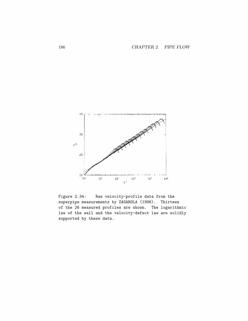
186 CHAPTER 2. PIPE FLOW
Figure 2.34: Raw velocity-profile data from the
superpipe measurements by ZAGAROLA (1996). Thirteen
of the 26 measured profiles are shown. The logarithmic
law of the wall and the velocity-defect law are solidly
supported by these data.
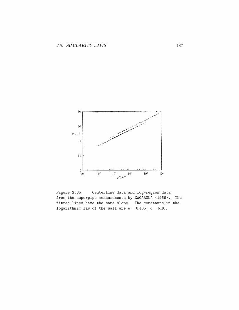
2.5. SIMILARITY LAWS 187
Figure 2.35: Centerline data and log-region data
from the superpipe measurements by ZAGAROLA (1966). The
fitted lines have the same slope. The constants in the
logarithmic law of the wall are κ = 0.435, c = 6.10.
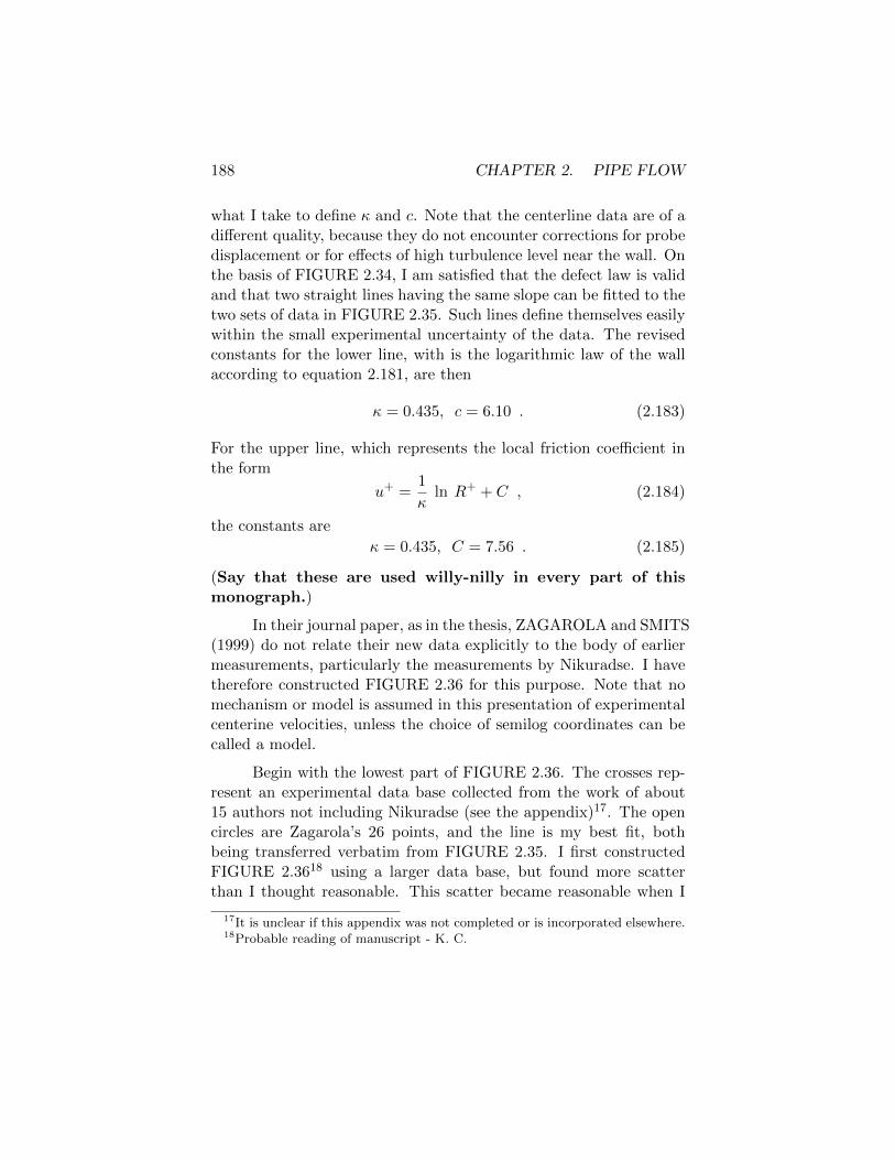
188 CHAPTER 2. PIPE FLOW
what I take to define κ and c. Note that the centerline data are of adifferent quality, because they do not encounter corrections for probedisplacement or for effects of high turbulence level near the wall. Onthe basis of FIGURE 2.34, I am satisfied that the defect law is validand that two straight lines having the same slope can be fitted to thetwo sets of data in FIGURE 2.35. Such lines define themselves easilywithin the small experimental uncertainty of the data. The revisedconstants for the lower line, with is the logarithmic law of the wallaccording to equation 2.181, are then
κ = 0.435, c = 6.10 . (2.183)
For the upper line, which represents the local friction coefficient inthe form
u+ =1
κln R+ + C , (2.184)
the constants are
κ = 0.435, C = 7.56 . (2.185)
(Say that these are used willy-nilly in every part of thismonograph.)
In their journal paper, as in the thesis, ZAGAROLA and SMITS(1999) do not relate their new data explicitly to the body of earliermeasurements, particularly the measurements by Nikuradse. I havetherefore constructed FIGURE 2.36 for this purpose. Note that nomechanism or model is assumed in this presentation of experimentalcenterine velocities, unless the choice of semilog coordinates can becalled a model.
Begin with the lowest part of FIGURE 2.36. The crosses rep-resent an experimental data base collected from the work of about15 authors not including Nikuradse (see the appendix)17. The opencircles are Zagarola’s 26 points, and the line is my best fit, bothbeing transferred verbatim from FIGURE 2.35. I first constructedFIGURE 2.3618 using a larger data base, but found more scatterthan I thought reasonable. This scatter became reasonable when I
17It is unclear if this appendix was not completed or is incorporated elsewhere.18Probable reading of manuscript - K. C.
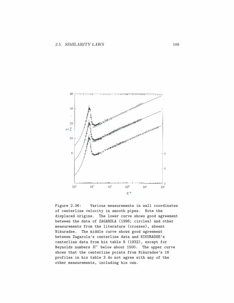
2.5. SIMILARITY LAWS 189
Figure 2.36: Various measurements in wall coordinates
of centerline velocity in smooth pipes. Note the
displaced origins. The lower curve shows good agreement
between the data of ZAGAROLA (1996; circles) and other
measurements from the literature (crosses), absent
Nikuradse. The middle curve shows good agreement
between Zagarola’s centerline data and NIKURADSE’s
centerline data from his table 8 (1932), except for
Reynolds numbers R+ below about 1500. The upper curve
shows that the centerline points from Nikuradse’s 16
profiles in his table 3 do not agree with any of the
other measurements, including his own.

190 CHAPTER 2. PIPE FLOW
discarded all data for which the necessary measurements of pressureor velocity were made closer to the pipe entrance than 100 diameters.
In passing, observe that the transition range is well defined bythe work of SENECAL (1953) and PATEL and HEAD (1969). Asquare-cut entrance appears to be an adequate tripping device at allReynolds numbers. (check) The beginning of transition is abrupt,at about R+ = 60, or Re = 2100, but the end of transition is not sowell defined, probably because of a slow approach to equilibrium. Asa test for final equilibrium, it would be useful to have flatness-factordata for velocity fluctuations on the pipe axis far downstream overa range of Re from 2000 to perhaps 10,000, to verify the disappear-ance of the bimodal laminar/turbulent probability-density functionassociated with intermittency. (See SECTION X on transition).
In the lowest part of FIGURE 2.36, where the old and newdata overlap, there is good agreement, although the straight line inthe figure may not be the best overall representation in the early partof the turbulent regime, below R+ = 103.
The central part of FIGURE 2.36 repeats part of the database and repeats the fitted line, but replaces Zagarola’s centerlinedata by Nikuradse’s centerline data from table 8 of his 1932 paper.At least for R+ greater than about 2000, there is no appreciabledifference between the two sets of measurements, despite the lowerlength/diameter ratio for Nikuradse’s pipes. However, for the low-est Reynolds numbers Nikuradse’s values seem low, indicating thattransition may have been over-tripped in this region.
Finally, the upper part of FIGURE 2.36 shows Nikuradse’scenterline points from the profiles in his table 3, together with thebase data and Zagarola’s straight line. There is a discrepancy inslope that (give value) is evidently internal to Nikuradse’s workand cannot be ignored. I have found nothing in his 1932 paper toexplain his difficulty with the rule that an experimenter must be ableto repreat his own measurements, and I suspect that the values of uτfor the profiles have been adjusted. There is more on this questionin SECTION X. (Check profiles of 1930 against 1932.)

2.5. SIMILARITY LAWS 191
2.5.8 The defect law
(Discuss as outer component in a singular-perturbation argument.Combine with next section? Validity depends on smoothness of uc/uτagainst ln Ruτ/ν.)
2.5.9 The limit Re→∞
A philosophical question about turbulent pipe flow concerns the limitof infinite Reynolds number. The defect law in the limit representsa square profile with a boundary layer at the wall (what about thewake component?). The turbulence is mixing so effectively that thereis no gradient in mean velocity. The problem looks like a classicalsingular perturbation problem, except that the equations are notknown. Several people have tried this problem. A reasonable test isto ask how the logarithm gets into the analysis, and the answer sofar is that the authors put it in, by one device or another. I thinkthis is an important exercise, and should be done correctly from thebeginning. Plot uτ/uc against 1/ln (Ruc/ν) and argue Cf → 0 asRe→∞?
The atmosphere is a boundary layer at very large Reynoldsnumber. There is only a wall component, since there is no way todefine a thickness or a free-stream velocity. One problem is that theflow should be neutrally stable. Another is that the effect of theearth’s rotation on the flow near the surface should be negligible.Another is that the surface should be smooth, and in practice thismeans smoother than smooth concrete. A last problem is that theapproaching flow should have a long fetch. (Look at meteorologicalliterature.)
2.5.10 The formal friction law
Karman (ref) noted the local friction law obtained by evaluatingthe profile formula (2.117) on the pipe axis, with a slightly different
192 CHAPTER 2. PIPE FLOW
constant,ucuτ
=1
κlnRuτν
+A . (2.186)
He applied this formula to estimate κ = 0.38 from Nikuradse’s datafor uc, uτ , and R in a smooth pipe. The fact that uc rather thanu appears here prevents any direct connection with the bulk of pipedata. (Use profile formula for uc/uτ . Document behavior at low Re.Try Burke again. How to replace uc by u?)
2.5.11 The Reynolds stresses
(Plot fluctuations in sublayer for y+ = 15, 50; also centerline values.See Lehigh paper.) Perry and Abell are looking for evidence that theturbulent fluctuations obey a wall/wake decomposition like the meanvelocity.
(Two topics so far are sudden area change; see Krall, Bogerand Halmos, and Khezzar et al, and effect of coiling, especially ontransition; see Taylor, White, Sreenivasan. Another is non-steadypipe-flow. Mention that roughness and polymers are treated sepa-rately.)
2.6 Roughness
2.6.1 Friction
Most of the early data on flow in pipes, from about 1860 to about1900, were obtained by civil engineers in pipes characteristic of waterdistribution systems, long vehicular tunnels and even sewers. Thesepipes were typically made of wood, riveted iron (sometimes corru-gated), cast iron or cast concrete, or excavated rock, and they oftendeteriorated over time because of accumulating corrosion or otherdeposits. Thus engineers lived with rough surfaces, and they tendedto carry out their experiments in the same circumstances where theinformation was to be applied. In the absence of any formalism for

2.6. ROUGHNESS 193
organizing their knowledge, they were simply good engineers. Col-lections of some of these early measurements can be found in papersby Blasius, Ombeck, and others. (Mention others.)
The Reynolds numbers in the early work were often large, andthe evidence showed that the pressure drop in a given pipe tended tovary as the square of the flow velocity, although exponents closer to7/4 were sometimes reported for especially smooth and clean pipes.Work on pipe flow as a classical problem in turbulent shear flowbegan near the end of the 19th century, and some of this work is citedin SECTION X. Work on the effects of roughness lagged, there beingno systematic studies taking into account geometric similarity andother questions of good experimental definition until the appearanceof a remarkable contribution by Nikuradse in 1933. This paper byNikuradse is still considered to be the seminal work on the problemof surface roughness, although there are several open questions to betaken later.
The discussion here begins where the subject ends, with thesubject of the fully rough regime. The main effect of large wallroughness is to replace the condition τw = µ(∂u/∂y)w by a dragcondition that treats three-dimensional roughness elements as bluffbodies, with a local pressure drag that is quadratic in some charac-teristic velocity u and independent of viscosity. If N is the numberof such elements and F is the total drag force, both per unit area,write approximately
F = CDρu2
2Nk2 = ρu2
τ , (2.187)
where CD is a drag coefficient and k is a roughness scale, to be definedlater.
For packed roughness, Nk2 is of order unity. If CD is also oforder unity, as it is for a sphere, say, at a Reynolds number uk/νgreater than about 1000, then u should be of order uτ (check thiswith real data). Moreover, if CD is independent of Reynolds num-ber, so is
Cf =F
12ρu
2≈ CD
(u
u
)2
, (2.188)
194 CHAPTER 2. PIPE FLOW
where u is a suitable external or reference velocity. This propertydefines the fully rough regime.
(If roughness is not packed, try a linear combination of the twoforms for F? 2D vs 3D? Who first understood roughness?)
A more elegant approach is in terms of similarity laws for themean-velocity profile, as these laws developed in connection with flowin smooth pipes. A useful point of attack is the defect law outsidethe sublayer,
uc − uuτ
= g( yR
), (2.189)
which does not involve the viscosity and was in fact proposed inde-pendently by several authors, beginning with DARCY (1858). Thisempirical law does not depend on the mechanism by which the re-tarding force F acts at the wall.
Now consider the law of the wall as a product of the mixing-length argument. This law emerged first in the form
u
uτ=
1
κln
y
y0, (2.190)
without giving any information about the nature of the constant ofintegration y0. If this constant depends only on conditions at thewall, then for a smooth wall the only possible form is
y0 =1
A
ν
uτ, (2.191)
where A is a constant. Equation (2.190) becomes
u
uτ=
1
κlnyuτν
+1
κlnA . (2.192)
For a fully rough wall, on the premise that the viscosity isirrelevant, the most obvious choice is
y0 =1
Bk , (2.193)
where B is another constant. Instead of equation (2.192), there isobtained
u
uτ=
1
κlny
k+
1
κln B . (2.194)
2.6. ROUGHNESS 195
Let the last expression be rewritten in the customary wall variablesas
u
uτ=
1
κlnyuτν− 1
κlnkuτν
+1
κlnB . (2.195)
Each of the four relationships so far given for u/uτ , if it is valid tothe pipe center, is consistent with the defect law (2.189).
Finally, consider the difference between equations (2.192) and(2.195). The vertical displacement of the logarithmic profile at afixed value of yuτ/ν, on subtraction of equation (2.192) from equa-tion (2.195), is
∆
(u
uτ
)= −1
κlnkuτν
+1
κlnB − 1
κlnA . (2.196)
Nikuradse’s data are central to all of these relationships. Onefigure corresponds to equation (2.194) and gives a value (1/κ) lnB =8.5, where data in smooth pipes according to equation (2.192) gave(1/κ) lnA = 5.0 (see SECTION X). The expectation is therefore thatthe profile shift in the fully rough regime should be described by
∆
(u
uτ
)= −1
κlnkuτν
+ 3.5 . (2.197)
Nikuradse gives this result in a different and less universal form. Therepresentation (2.197) has become standard since it was first plottedby (who?).
FIGURE X19 shows Cf as a function of Re for Nikuradse’s ex-periments. What is obvious and impressive is that the roughnessesused by Nikuradse have no effect on laminar flow or on transition, oreven on turbulent flow, until a critical roughness (which depends onReynolds number) is exceeded. Then there is a departure from thesmooth curve and an eventual quadratic drag behavior above anothercritical Reynolds number (note that Cf and u/u or uτ/u are inde-pendent of Re here). In terms of the vertical displacement of the ve-locity profile, the same behavior is shown in FIGURE X. The effectsof roughness are first felt at roughly kuτ/ν = 5, where the roughness
19Figures cited in this paragraph are missing.
196 CHAPTER 2. PIPE FLOW
elements begin to project beyond the linear part of the smooth-wallprofile, and the fully rough behavior occurs for kuτ/ν > 70, whichis, by coincidence or otherwise, approximately the thickness of thesublayer for a smooth wall. The slope is 1/κ as it should be.
All of this is conventional wisdom and appears in numerousbooks. A number of questions need discussion in the light of thewhole literature of the subject.
(1) What is meant by “mean velocity”? How is it to be de-fined below the top of the roughness? By a mean over a planey = constant? There are no data in what used to be the sublayer.
(2) What happens to maintain the velocity at the center of thepipe, uc/uτ , when the profile displacement becomes very large? Isthere a limiting behavior?
(3) How should k be defined, and also R, for the roughness?How does B in equation (27.13) depend on k? Where should the ori-gin be taken for y? Is a volume criterion generally useful, as proposedby Nikuradse? See Clauser. What about rib and slot roughness?
These issues are attached to the mixing-length argument, whichis implausible. However, it is an occasional success like this one thatkeeps the mixing length alive. It is astonishing that roughness isunder such good control. The defect law is a clue.
(Comment on Nikuradse problem and cite paper on boundarylayers. The man who wrote that paper was not bright enough toinvent the roughness data, which have been tested and accepted asreal by dozens of investigators, including me.)
(Pipeline people are consumers of information, not producers.The cost of making and maintaining smooth pipe is probably greaterthat the cost of pumping through a commercially rough pipe.)

2.7. POLYMERS 197
2.7 Polymers
2.7.1 Friction
Two problems that seem at least superficially to be related are theeffects of surface roughness and the effects of high-molecular-weightpolymers on flow of liquids past a smooth wall. Most of the workwith polymers has been carried out in pipe flow, because the surfacefriction can be unambiguously determined from the pressure gradi-ent.
It was discovered independently by two groups about 1945 thata very dilute solution of a long-chain polymer in a suitable solventhas remarkable properties in reducing the pressure loss in pipe flow.Important names include Metzner and Virk for the period 1965-1975when most of the work was done.
Difficulties include degradation by pumps, so that the mostsystematic data have been obtained in one-pass systems. Temper-ature matters; so does pH. There are problems with probes, eitherhot-film or pitot-static probes. Mixing of solutions requires care.The LDV is hard to use in a circular pipe.
Taylor’s four-roller apparatus is sometimes used to generate astrain field for studying the question of a critical velocity or a criticalstrain rate.
A characteristic dimensionless number is the Deborah number,
De = ετ (2.198)
where ε is strain rate and τ is some characteristic physical or chemicaltime for the polymer. A packed bed of particles can be used for thesame purpose.
The effect of a polymer is to raise the logarithmic part of themean velocity profile, as if there exists a concept of negative rough-ness. The effect on the friction coefficient is to cause a decrease,toward but never to the curve for laminar flow. Virk has a speciallimit curve.
198 CHAPTER 2. PIPE FLOW
It is very difficult to make this association plausible, exept thatroughness and polymer both affect primarily the flow in the sublayer.
Remarks on handout.
Most experiments use gravity-fed pipe flow.
Tomita. This is the same pipe and same polymer. Figure 5 showscritical shear rate constant but R changing? Figure 6 shows limitindependent of polymer (see Virk).
Huang. Used cone-plate viscometer to measure ν independently.Tubes tend to be very small, to fit in a bath, and involve very largepressure drops. Solutions remain Newtonian at concentrations used.Figure 9: note ∆u/uτ is proportional to square root of concentration.
Janberg. Nice velocity profiles; also temperature.
Van Driest. Neglected paper. Note high concentrations. Guar gumis not Newtonian for concentrations above one percent. Note thattransition is independent of concentration. Note Fig. 21 for asbestosfibers.
White. Used smooth and rough pipes. Figures 5 and 6 show reversalof effect. Soap also reverses (Fig. 7).
Mizushina and Usui. LDV data do not check asymptotic sublayer.
Rollin and Seyer. Used particle tracing to get profiles. See particu-larly sublayer profile.
Spangler. Profiles look strange. Derive coordinates in Fig. 6. In Fig.7b, slope is wrong for polymer.
Virk. Friction asymptote is purely empirical. It has an effect on theprofile also. There is some kind of saturation.
2.7.2 Mean velocity
2.7.3 Re Stresses
2.8. HEAT TRANSFER 199
2.8 Heat transfer
2.8.1 Friction
2.8.2 Mean temperature
2.8.3 Consensus on heat transfer
2.9 Variations on classical pipe flow
2.9.1 Odd shapes
2.9.2 Coiled pipes
2.9.3 Area change
2.9.4 Non-steady flow
2.9.5 Swirl
2.9.6 Wall suction, blowing