Topics in Health and Education Economics –...
38
1 Topics in Health and Education Economics – class2 Matilde P. Machado [email protected] Matilde Pinto Machado 2.2. Adverse Selection/Risk Selection Rothschild & Stiglitz (QJE,1976) Summary: Shows the impact of imperfect information on the equilibrium outcome of a competitive insurance market. Insurance companies offer insurance contracts that rely on a self-selection mechanism High risk individuals cause an externality on low risk individuals Everyone would be better off (or as well off) if risks were revealed ex-ante.
Transcript of Topics in Health and Education Economics –...

1
Topics in Health and Education Economics – class2
Matilde P. [email protected]
Matilde Pinto Machado
2.2. Adverse Selection/Risk SelectionRothschild & Stiglitz (QJE,1976)
Summary:
� Shows the impact of imperfect information on the equilibrium outcome of a competitive insurance market.
� Insurance companies offer insurance contracts that rely on a self-selection mechanism
� High risk individuals cause an externality on low risk individuals
� Everyone would be better off (or as well off) if risks were revealed ex-ante.

2
Matilde Pinto Machado
2.2. Adverse Selection/Risk Selection Rothschild & Stiglitz (QJE,1976)
Model I – the case of a single type of consumer:
� There are two states of nature {no accident, accident}.
� No insurance: wealth = {W,W-d}
� p ≡ probability of accident occurring
� α=(α1,α2) is the insurance vector where α1 is the premium paid by the consumer and α2 is the net compensation in case of accident, i.e. α2 = q-α1 where q is the insurance coverage.
� With insurance: wealth = {W-α1,W-d+ α2}
Matilde Pinto Machado
2.2. Adverse Selection/Risk Selection Rothschild & Stiglitz (QJE,1976)
1. Supply side of the insurance market:
� Insurers are risk-neutral, they maximize expected profits
� Perfect competition ⇒ Expected profit = 0
(A) 1
0)1(),( 1221 αααααπp
pppp
−=⇔=−−=
Expected profit of selling contract α to individuals with probability of accident = p
Competitive relation between the net compensation and the premium
3
Matilde Pinto Machado
2.2. Adverse Selection/Risk Selection Rothschild & Stiglitz (QJE,1976)
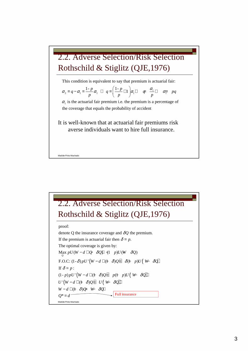
It is well-known that at actuarial fair premiums risk averse individuals want to hire full insurance.
12 1 1 1 1
1
This condition is equivalent to say that premium is actuarial fair:
1 1 1
is the actuarial fair premium i.e. the premium is a percentage of
the coverage that e
- p - pq q q pq
p p p
αα α α α α
α
= − = ⇔ = + ⇔ = ⇔ =
quals the probability of accident
Matilde Pinto Machado
2.2. Adverse Selection/Risk Selection Rothschild & Stiglitz (QJE,1976)
( ) ( )
proof:
denote Q the insurance coverage and the premium.
If the premium is actuarial fair then .
The optimal coverage is given by:
Max ( ) (1 ) ( )
F.O.C: (1- ) ' (1 ) (1 ) '
Q
Q
p
pU W d Q Q p U W Q
pU W d Q p U W Q
δδ
δ δ
δ δ δ δ
=
− + − + − −
− + − = − −
( ) ( )( ) ( )
If :
(1- ) ' (1 ) (1 ) '
' (1 ) '
(1 )
*
p
p pU W d Q p p U W Q
U W d Q U W Q
W d Q W Q
Q d
δδ δ
δ δδ δ
=− + − = − − ⇔
− + − = − ⇔− + − = − ⇔= Full insurance

4
Matilde Pinto Machado
2.2. Adverse Selection/Risk Selection Rothschild & Stiglitz (QJE,1976)
W2
Wealth after accident
45º
W1>W2
W2>W1
W1 Wealth with no accident
W1=W2 Full insurance combinations
relevant
Matilde Pinto Machado
2.2. Adverse Selection/Risk Selection Rothschild & Stiglitz (QJE,1976)� All wealth combinations along EF are feasible (i.e. Expected profit=0). F
is the feasible point of Complete insurance
W1
No accident
45º
W2=W1 (Completely insured)
W1>W2
W2>W1
W2
(with accident)
E
Wealth without insurance
Possible wealth combinations with competitive insurance, slope= - (1-p)/p
W-d
W
F

5
Matilde Pinto Machado
2.2. Adverse Selection/Risk Selection Rothschild & Stiglitz (QJE,1976)
Derivation of EF line:
1 1 1 1
2 2 1 1
2 1
1 2
22 2 2 1
Wealth with NO accident :
1 1With accident: ( )
1 1 EF line, slope =
Therefore when
1
α α
α α
= − ⇔ = −− −= − + = − + = − + −
− −= − − ⇔ −
=−= − − ⇔ = − ⇔ = − =
W W W W
p pW W d W d W d W W
p p
W p pW d W
p p p
W W
WW p WW d W d W W pd W
p p p p
Matilde Pinto Machado
2.2. Adverse Selection/Risk Selection Rothschild & Stiglitz (QJE,1976)Definition of Equilibrium: The equilibrium in a
competitive insurance markets is a set of contracts such that:
(i) No contract in the equilibrium set makes negative profits
(ii) There is no contract outside the set that, if offered, would make no-negative profits.
We know that when the premium is actuarial fair, risk averse prefer F to the rest of the possible wealth combinations, i.e. complete insurance.

6
Matilde Pinto Machado
2.2. Adverse Selection/Risk Selection Rothschild & Stiglitz (QJE,1976)2. Demand Side of the Insurance Market
� Individuals maximize their expected utility that depends only on their wealth
� Individuals know p
� Their utility function is state independent
� Their expected utility function is:
2 1( ) (1 ) ( )pU W p U W+ −
Matilde Pinto Machado
2.2. Adverse Selection/Risk Selection Rothschild & Stiglitz (QJE,1976)The slope of the indifference curve at F equals the slope of
EF line. F is therefore the optimum point (highest i.c.) in EF.
[ ]
( )
1 2
1 2
2 11 1 2 2
1 2
1 2
2
1
0 (1 ) ( ) ( )
( )11 ( ) ( ) 0
( )
At F, (complete coverage) Thus:
1
W W
dUE d p U W pU W
dW U Wpp U W dW pU W dW
dW p U W
W W
dW p
dW p=
= = − + =′−′ ′− + = ⇔ = −′
=
−= −The slope of the indifference curve at W1=W2 is independent of U(.) and the same as the EF line. The tangency of the indifference curve to EF shows that individuals maximize their expected utility at F.

7
Matilde Pinto Machado
2.2. Adverse Selection/Risk Selection Rothschild & Stiglitz (QJE,1976)The equilibrium:
W1
45º
W2=W1 (total insurance)W2
E
F
Optimal premium=α∗1
α*2
W-d
W
Optimal net compensation
Matilde Pinto Machado
2.2. Adverse Selection/Risk Selection Rothschild & Stiglitz (QJE,1976)For α*=(α* 1, α* 2) to be an equilibrium we need to
check that it satisfies the two previous conditions which amount to:
� BE=0 (The wealth combination must be along the EF line)
� Any other insurance contract (a1,a2) that consumers may prefer has negative benefits <0. Those would be contracts that lead to wealth combinations in higher indifference curves and obviously those are lower premium for the same (or higher) compensation or higher compensations for the same (or lower) premium which yield negative expected profits.

8
Matilde Pinto Machado
2.2. Adverse Selection/Risk Selection Rothschild & Stiglitz (QJE,1976)Model II – the case of two types of consumers:- Low Risk – probability of accident = pL
- High Risk – probability of accident = pH
- pH > pL
− λ ≡ proportion of high risks 0<λ<1
- Individuals know their types and their probability of accident
- Individuals only differ in their risk, the insurance company cannot distinguish them ex-ante, however the insurer knows the values of pH , pL and λ.
(1 ) average prob. of accidentH Lp p pλ λ= + − ≡
Matilde Pinto Machado
2.2. Adverse Selection/Risk Selection Rothschild & Stiglitz (QJE,1976)- The insurance company knows that for the same
premium, high risks would like to hire more coverage. It will use this information to devise self-selection mechanisms.
- Individuals cannot buy more than one insurance contract
- There can only be two types of equilibrium:- Pooling – both types buy the same contract
- Separating – Each type buys a different contract
It can be shown that a Pooling Equilibrium never exists.

9
Matilde Pinto Machado
2.2. Adverse Selection/Risk Selection Rothschild & Stiglitz (QJE,1976)
Proof that a Pooling Equilibrium never exists.By contradiction, suppose α=(α1, α2) is a pooling
equilibrium, in that case, it can be shown that Exp. Profits are a function of the average prob. of accident:
[ ] [ ][ ]( ) ( )
1 2 1 2
1 2 2
1 2
1 2
( , ) (1 ) (1 ) (1 )
(1 ) (1 )(1 ) (1 )
(1 ) (1 ) (1 )
(1 )
H H L L
H L H L
H L H L
p p p p p
p p p p
p p p p
p p
π α λ α α λ α αλ λ α λ α λ αλ λ λ λ α λ λ α
α α
= − − + − − − =
= − + − − − − −
= − + − − − − + −= − −
Matilde Pinto Machado
2.2. Adverse Selection/Risk Selection Rothschild & Stiglitz (QJE,1976)
The rate of substitution between the two states of nature can be derived for the high risks:
And similarly for the low risks:
( )( )
)´(
)´()1(
)´(
)´()1(
0)´()´(10
)()(1
2
1
2
1
1
2
2211
21
αα
α +−−−−=−−=⇔
=+−⇔=
+−=
dWUp
WUp
WUp
WUp
dW
dW
dWWUpdWWUpdUE
WUpWUpUE
H
H
H
H
H
HHH
HHH
)´(
)´()1(
)´(
)´()1(
2
1
2
1
1
2
αα
α +−−−−=−−=
dWUp
WUp
WUp
WUp
dW
dW
L
L
L
L
L

10
Matilde Pinto Machado
2.2. Adverse Selection/Risk Selection Rothschild & Stiglitz (QJE,1976)
So the difference of the rate of substitution for high and risks only depends on the probabilities:
2 2
1 1
1 1
and
1 1
1 1 1 11 and
H LH L
H L
H L H L
H L H L
H L
p pp p
p p
p p p pp
p p p p p
dW dW
dW dWα α
> ⇒ <
− < −− − − −−
⇒ < < <
<The indifference curve of the Low risks (for the equilibrium contract α) is steeper in absolute terms.
Matilde Pinto Machado
2.2. Adverse Selection/Risk Selection Rothschild & Stiglitz (QJE,1976)
W1
45º
W2=W1W2
W-d
W
UH
UL
Note that EF has now a slope that depends on the average prob. of accident
Fα
Note that α must be in the EF curve so that the expected profit is =0

11
Matilde Pinto Machado
2.2. Adverse Selection/Risk Selection Rothschild & Stiglitz (QJE,1976)
The existence of a contract β shows that α is not an eq.
W1
45º
W2=W1W2
W-d
W
UH
UL
β is preferred to α by the low risk and since it is in EF or even slightly above can be offered in the market (because only low risks would buy it).
F
0),(),(),( =>≈ απαπβπ ppp LL
α
Matilde Pinto Machado
2.2. Adverse Selection/Risk Selection Rothschild & Stiglitz (QJE,1976)If an equilibrium exists it MUST be separating. They
assume that there is no cross-subsidization, i.e. competition forces the insurance company to break even for every contract. The zero expected profit conditions are now given by:
Which imply two different wealth combination lines from the initial E point.
1 2 2 1
1 2 2 1
1( , ) (1 ) 0 (B1)
1( , ) (1 ) 0 (B2)
LL L L L L L L L
L
HH H H H H H H H
H
pp p p
p
pp p p
p
π α α α α α
π α α α α α
−= − − = ⇔ =
−= − − = ⇔ =

12
Matilde Pinto Machado
2.2. Adverse Selection/Risk Selection Rothschild & Stiglitz (QJE,1976)For the same premium the insurance company could offer a much higher net compensation to the low risks.
1 L
L
p
p
−−
W1
45º
W2=W1W2
H
L
E
Premium =a
Slope EL:
Slope EH:1 H
H
p
p
−−Measures competitive net compensation for high and low risks for a premium = a
Matilde Pinto Machado
2.2. Adverse Selection/Risk Selection Rothschild & Stiglitz (QJE,1976)However H and L do not constitute an equilibrium
45º
W2
H
LUH
αH E
θ
0),( ;0),( == θπαπ LHH pp
Of all wealth combinations along EH, αH is the preferred one by the high risks. And of all those along EL, θ is the preferred by the low risks. We know that Eπ=0 if αH is sold to the high risks and θ to the low risks. The problem is that θis also preferred to αHby the high risks since it means higher wealth in both states of nature.
U’H

13
Matilde Pinto Machado
2.2. Adverse Selection/Risk Selection Rothschild & Stiglitz (QJE,1976)And the insurer will have negative expected profits if it sells θ to everyone. That is if all individuals buy the contract θ then:
45º
W2
αH
LUH
E
θ
U’H
0),(),( =< θπθπ Lpp
Matilde Pinto Machado
2.2. Adverse Selection/Risk Selection Rothschild & Stiglitz (QJE,1976)The segment between EαL shows the set of wealth combinations that could be offered to the low risks at zero expected profit and are NOT preferred to αH by the high risks (incentive compatibility constraint)
The set of candidates to an equilibrium is αΗ and contracts along EαL . Of all those along EαL , αL is the preferred by the low risk. So we will check under which conditions {αΗ ,αL} is an equilibrium.
45º
W2
αH
LUH
E
θ
αL
UL

14
Matilde Pinto Machado
2.2. Adverse Selection/Risk Selection Rothschild & Stiglitz (QJE,1976)
To prove that {αH, αL} is indeed an equilibrium: The first condition is satisfied because the insurer has expected zero profit in both contracts. The second condition is the difficult one. The existence of equilibrium depends on the percentage of high risks, λ. It turns out that if λis high enough there is an equilibrium, otherwise there isn’t.
Matilde Pinto Machado
2.2. Adverse Selection/Risk Selection Rothschild & Stiglitz (QJE,1976)Suppose γ is also offered. Then all individuals would prefer γ to the eq. candidate. The question is can γ be offered in the market? For {αH,αL} to be an equilibrium, the exp. profit from γ should be <0.
45º
W2
UL
H
LUH
αH E
θ
γαL
The expected profit from is given by: (, )pγ π γ

15
Matilde Pinto Machado
2.2. Adverse Selection/Risk Selection Rothschild & Stiglitz (QJE,1976)For a low level of λ, the line of possible wealth combinations achieved with contracts that are sold to both types and breakeven is near EL for example EF2. If λ is high then the line is somewhere close to EH e.g. EF1.
45º
W2
UL
UH
αH
E
θ
γ
F2
F1
For the high value of λ (EF1) γ cannot be offered at a profit so {αH,αL} is an equilibrium. For a low of λ (EF2) there is no equilibrium in this competitive market.
Matilde Pinto Machado
2.2. Adverse Selection/Risk Selection Rothschild & Stiglitz (QJE,1976)Conclusions:� the incomplete information may cause a
competitive market to have no equilibrium� The high risks are a negative externality on
the low risks� Everyone would be at least as well off if
everyone revealed their type

16
Matilde Pinto Machado
2.2. Adverse Selection/Risk Selection Olivella, Vera-Hernández (WP06/02)This paper is nice because:
� It is an application of R&S
� It uses data!! (The British Household Panel Survey)
� It tests adverse selection in a market where there are private health insurers on top of a National Health Service (NHS).
� They find evidence of adverse selection in the private insurance market
Matilde Pinto Machado
2.2. Adverse Selection/Risk Selection Olivella, Vera-Hernández (WP06/02)Setting: The British Private Health Insurance Market.� What’s especial?
� There is a public system that covers all expenditures(no copayments with few exceptions e.g. dental) and everyone.
� If people want to they can hire a private insurance. Private and Public are then substitutes for care. Everyone contributes to the public system through taxes.
� Other systems such as most of the American is purely private (except for Medicare/Medicaid)
� In other systems, the private is supplementary, people hire the private to cover for copayments and services not covered by the public (Belgium, France).

17
Matilde Pinto Machado
2.2. Adverse Selection/Risk Selection Olivella, Vera-Hernández (WP06/02)� Model:
� Individuals decide whether to take private insurance after observing their type and before becoming ill.
� Individuals when become ill must choose where they want to be treated (private/public) and private and public services cannot be combined.
� If an individual chooses the private service, the private insurer must cover the full cost.
� Everyone contributes to the financing of the public health service regardless of whether he/she uses the public health services (PUB).
� There are a large set of insurers (similar to R&S)� Individuals can be of one of two types {L,H}, 1>PH>PL>0 and they
know their type� γ≡ (1-λ) proportion of low risks, 0< γ<1
Matilde Pinto Machado
2.2. Adverse Selection/Risk Selection Olivella, Vera-Hernández (WP06/02)
� Model (timing):
Health authority chooses package
Private insurers simultaneously make their packages conditional on the package of the HA
Individuals decide whether or not to take private insurance, and which insurer, conditional on the packages of all providers and their type
18
Matilde Pinto Machado
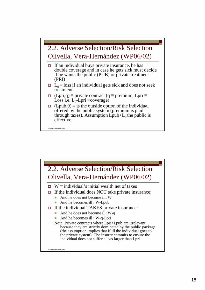
2.2. Adverse Selection/Risk Selection Olivella, Vera-Hernández (WP06/02)� If an individual buys private insurance, he has
double coverage and in case he gets sick must decide if he wants the public (PUB) or private treatment (PRI)
� L0 ≡ loss if an individual gets sick and does not seek treatment
� (Lpri,q) ≡ private contract (q ≡ premium, Lpri ≡ Loss i.e. L0-Lpri ≡coverage)
� (Lpub,0) ≡ is the outside option of the individual offered by the public system (premium is paid through taxes). Assumption Lpub<L0 the public is effective.
Matilde Pinto Machado
2.2. Adverse Selection/Risk Selection Olivella, Vera-Hernández (WP06/02)� W ≡ individual’s initial wealth net of taxes� If the individual does NOT take private insurance:
� And he does not become ill: W� And he becomes ill : W-Lpub
� If the individual TAKES private insurance:� And he does not become ill: W-q� And he becomes ill : W-q-Lpri Note: Private contracts where Lpri>Lpub are irrelevant
because they are strictly dominated by the public package (the assumption implies that if ill the individual goes to the private system). The insurer commits to ensure the individual does not suffer a loss larger than Lpri
19
Matilde Pinto Machado
2.2. Adverse Selection/Risk Selection Olivella, Vera-Hernández (WP06/02)
� If the individual does NOT take private insurance:� Expected utility for probability p is:
� If the individual TAKES private insurance:� Expected utility for probability p is:
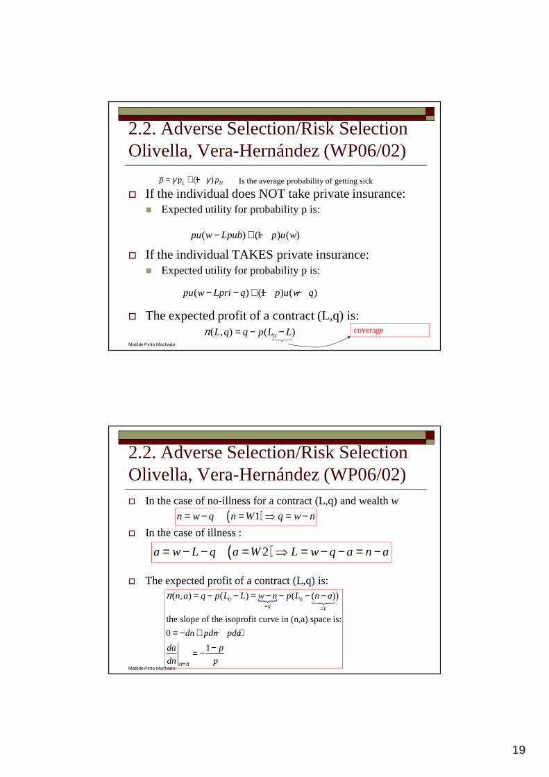
� The expected profit of a contract (L,q) is:
(1 )L Hp p pγ γ= + − Is the average probability of getting sick
( ) (1 ) ( )pu w Lpub p u w− + −
( ) (1 ) ( )pu w Lpri q p u w q− − + − −
0( , ) ( )L q q p L Lπ = − − coverage
Matilde Pinto Machado
2.2. Adverse Selection/Risk Selection Olivella, Vera-Hernández (WP06/02)� In the case of no-illness for a contract (L,q) and wealth w
� In the case of illness :
� The expected profit of a contract (L,q) is:
( ) 1n w q n W q w n= − = ⇒ = −
( ) 2a w L q a W L w q a n a= − − = ⇒ = − − = −
�0 0( , ) ( ) ( ( ))
the slope of the isoprofit curve in (n,a) space is:
0
1
q L
n a q p L L w n p L n a
dn pdn pda
da p
dn pπ π
π= =
=
= − − = − − − −
= − + − ⇔−= −
���

20
Matilde Pinto Machado
2.2. Adverse Selection/Risk Selection Olivella, Vera-Hernández (WP06/02)� We have 2 zero-isoprofit curves depending on the
individual’s type, with slopes:
� The zero-isoprofit curves go through point E = (w,w-L0) (i.e. no insurance)
0 0
1 1;
H L
H L
H L
p pda da
dn p dn pπ π= =
− −= − = −
�
0
0 00
( , ) ( ( )) 0L
n w a w L w n p L n aπ= =
= = − = − − − − =���
Matilde Pinto Machado
2.2. Adverse Selection/Risk Selection Olivella, Vera-Hernández (WP06/02)3.1. Symmetric Information
� If there is NO public system, then the equilibrium would be just as in R&S with symmetric information, i.e. efficient contracts or complete coverage to both types i.e. {α* L,α*H} i.e. for J=H,L
0
0 0
( , ) 0 ( ( )) 0
0
actuarial fair contracts.
J J
J J
n a w n p L n a n a
w n p L n w p L a
Π = ⇔ − − − − = ∧ =⇒ − − = ⇔ = − =

21
Matilde Pinto Machado
2.2. Adverse Selection/Risk Selection Olivella, Vera-Hernández (WP06/02)� In the presence of a public system the status-quo is
not E=(w,w-L0) but P=(w,w-Lpub)
45º
W2=a
α∗H
LUH
E
α∗L
W-L0
W-pHL0
W-pHL0
W-pLL0
W-pLL0
Possible positions of the public package.
If Lpub=L0
then E is the status quo with public coverage (i.e. it is as if the public system did not existed)
W1=nW
Matilde Pinto Machado
2.2. Adverse Selection/Risk Selection Olivella, Vera-Hernández (WP06/02)� Assumption 1: If all individuals of type J are
indifferent between the public package P and the best private contract for them, all these individuals choose the public package.

22
Matilde Pinto Machado
2.2. Adverse Selection/Risk Selection Olivella, Vera-Hernández (WP06/02)
In the presence of P=(w,w-Lpub) some private contracts (in the symmetric information eq.) may not be attractive any more
45º
a
α∗H
LUH
E
α∗L
W-L0
W-pHL0
W-pHL0
W-pLL0
W-pLL0
P1
P2
P3
If P=P1 then private market not affected, the public contract is NOT ACTIVE; If P=P2 α*H not attractive anymore; If P=P3 no private contract is attractive, the private market is NOT ACTIVE
n
a=n
Matilde Pinto Machado
2.2. Adverse Selection/Risk Selection Olivella, Vera-Hernández (WP06/02)� The equilibrium will depend on P
45º
W2
α∗H
LUH
E
α∗L
W-L0
W-pHL0
W-pHL0
W-pLL0
W-pLL0
H0
L0
Proposition 1: In case P is between E-H0 the equilibrium is {α*H,α*L}; if P lies between H0 and L0 the equilibrium is {P,α*L}, in case P lies strictly above L0 then only P exists

23
Matilde Pinto Machado
2.2. Adverse Selection/Risk Selection Olivella, Vera-Hernández (WP06/02)So if both sectors are active (i.e. P is between H0 and
L0) and there is no adverse selection the probability of illness among the ones with a private insurance ispL i.e. the low risk, lower than the average probability of illness.
Matilde Pinto Machado
2.2. Adverse Selection/Risk Selection Olivella, Vera-Hernández (WP06/02)3.2. Asymmetric Information� If there is NO public system, then the equilibrium
would be just as in R&S with asymmetric information, i.e. efficient contracts or complete coverage to the high risks and less than full coverage to the low risks
� We know that in R&S we need the proportion of high risks to be high enough so that there is equilibrium i.e. γ≤γ*
� Assumption 2: assume γ≤γ*
{ }*ˆ ,L Hα α

24
Matilde Pinto Machado
2.2. Adverse Selection/Risk Selection Olivella, Vera-Hernández (WP06/02)� The equilibrium will depend on P:
ˆLα
45º
W2
α∗H
LUH
EW-L0
W-pHL0
W-pHL0
W-pLL0
W-pLL0
H0
L1
Again H0 is the public contract such that a high risk is indifferent between the public contract and the private contract α*H. L1 is the public contract such that the low-risk is indifferent between P and . Note that H0 is above L1 (Lemma 2)ˆ
Lα
Matilde Pinto Machado
2.2. Adverse Selection/Risk Selection Olivella, Vera-Hernández (WP06/02)Case 1: P lies below L1 ⇒ eq is P is not active
Case 2-3: P coincides with L1 or is between L1 and H0 the equilibrium is {α*H,P} (assumption 2 is no longer necessary for the existence of the equilibrium.) Both Public and Private are ACTIVE.
Case 4-5: P coincides with H0 or is above H0, in the equilibrium only the public system exists.
If both sectors are active under adverse selection then the probability of illness of those who purchase private insurance is pH which is larger than the average probability of illness.
{ }*ˆ ,L Hα α

25
Matilde Pinto Machado
2.2. Adverse Selection/Risk Selection Olivella, Vera-Hernández (WP06/02)� Their Main Theoretical Result:
� When both markets are active i.e. the private and the public then, with perfect information (i.e. no adverse selection) only the low risk would buy private insurance
� When both markets are active i.e. the private and the public then, with asymmetric information and therefore adverse selection only the high risks would buy private insurance.
� i.e. the sign of the correlation between the probability of buying private insurance and individuals’ risk depends on whether there is adverse selection. This prediction can be tested.
Matilde Pinto Machado
2.2. Adverse Selection/Risk Selection Olivella, Vera-Hernández (WP06/02)
Empirical Test:
� In the UK the private system is substitute to the public one.
� Everyone is entitled to the public system, and people pay it through taxes regardless of utilization
� The private system offers better access, in particular negligible waiting times, in the model’s notation it is true that Lpub>Lpri
� Data: Bristish Household Panel Survey (BHPS)

26
Matilde Pinto Machado
2.2. Adverse Selection/Risk Selection Olivella, Vera-Hernández (WP06/02)Empirical Test (cont.): � In the UK, Private and Public systems are active so the
model tells us that:� In the absence of adverse selection (perfect information) only the
low risks buy private insurance� In the presence of adverse selection only the high risks buy private
insurance.� We could therefore design a test by comparing the risk of requiring
medical care of those that decide to buy medical insurance to those that decide not to buy it. However this would have problems:1. One does not observe whether people require medical care, only
observes whether people get medical care2. Access conditions are better in the private insurance so we could
observe more people getting medical care under private insurance and wrongly conclude they were more needy of care.
Matilde Pinto Machado
2.2. Adverse Selection/Risk Selection Olivella, Vera-Hernández (WP06/02)Empirical Test (cont.): � To avoid the bias that may be introduced because of
differences in access to care between private and public, they restrict the sample to individuals that have the same access to hospitalizations: restrict to individuals that have private insuranceand distinguish between:� Individuals who buy private insurance on their own� Individuals who have private insurance as a fringe benefit from their
employer (i.e. they get it for free)
� The test compares the probability of hospitalization of those who purchase private insurance to those who get it as a fringe benefit.
Note: as we mention in the previous class hospitalizations are likely to be free of moral hazard.

27
Matilde Pinto Machado
2.2. Adverse Selection/Risk Selection Olivella, Vera-Hernández (WP06/02)� They restrict the sample to England and to
employees employed on a permanent basis.
� The identification assumption is that the individuals that get private insurance as a fringe benefit (conditional on covariates) are of the same risk, on average as the population of english permanently employed, i.e. the health insurance is orthogonal to health status conditional on covariates such as age, education, gender and income.
Matilde Pinto Machado
2.2. Adverse Selection/Risk Selection Olivella, Vera-Hernández (WP06/02)� Potential bias:
� Employer driven: some jobs are more likely to offer employer-paid health insurance then others. If health of individuals in these different jobs differ (conditional on covariates) then we may be biasing the results. For example, in agriculture the % of employed paid individuals is only 15% while in the banking, finance, insurance, business sector is of 66%. By occupation, the % of managers with employer-paid private insurance is of 63% while for operators of plants and machines it is only 38%. To control for this possibility they include in the regressions industry and occupation among the covariates. This means that conditional on being of a certain occupation we compare the effect of buying private insurance.

28
Matilde Pinto Machado
2.2. Adverse Selection/Risk Selection Olivella, Vera-Hernández (WP06/02)
� Potential bias (cont.):� Employee driven: If less healthy people search
for jobs that offer private insurance. � Some evidence (no proof): Most people that changed
jobs offer reasons other than private insurance, for example, more money or better chances of promotion.
� In any case, this would imply a smaller difference in risks between the two groups (downwards bias) ⇒the true adverse selection would be even higher than what they find.
Matilde Pinto Machado
2.2. Adverse Selection/Risk Selection Olivella, Vera-Hernández (WP06/02)
� The idea is:
Pool of permanently employed
Get insurance as Fringe Benefit
Do not Get insurance as Fringe Benefit
Conditional on X, same average prob of Hospitalization, pbar
Buy insurance Don’t Buy
Different risksComparison in the data
29
Matilde Pinto Machado
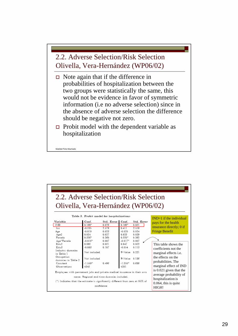
2.2. Adverse Selection/Risk Selection Olivella, Vera-Hernández (WP06/02)
� Note again that if the difference in probabilities of hospitalization between the two groups were statistically the same, this would not be evidence in favor of symmetric information (i.e no adverse selection) since in the absence of adverse selection the difference should be negative not zero.
� Probit model with the dependent variable as hospitalization
Matilde Pinto Machado
2.2. Adverse Selection/Risk Selection Olivella, Vera-Hernández (WP06/02)
IND=1 if the individual pays for the health insurance directly; 0 if Fringe Benefit
This table shows the coefficients not the marginal effects i.e. the effects on the probabilities. The marginal effect of IND is 0.021 given that the average probability of hospitalization is 0.064, this is quite HIGH!

30
Matilde Pinto Machado
2.2. Adverse Selection/Risk Selection Olivella, Vera-Hernández (WP06/02)Probit model – review:
1 if 0 where ~ (0,1) (the variance cannot be identified)
0 otherwise
Pr( 1) Pr( ) ( ) ( )
( ) 1 Pr( 1) 0 (1 Pr( 1)) Pr( 1) ( )
Therefore the marginal
i
i i i i
i
x
i i i i
i i i i
y x N
y
y x t dt x
E y y y y x
β
β ε ε
ε β φ β
β
′
−∞
′= + >=
′ ′= = > − = = Φ
′= × = + × − = = = = Φ
∫
effects for the probit are:
( )( ) - usually evaluated at the average value of in the samplei
i
E yx x
xφ β β β∂ ′ ′=
∂
Matilde Pinto Machado
2.2. Adverse Selection/Risk Selection Olivella, Vera-Hernández (WP06/02)
� Their test of adverse selection concludes that individuals that purchase private insurance have a higher probability of hospitalizations (are higher risk) than individuals that have private insurance as a fringe benefit. This constitutes evidence of adverse selection in the British private medical insurance market.

31
Matilde Pinto Machado
2.2. Adverse Selection/Risk Selection Olivella, Vera-Hernández (WP06/02)
� Robustness:� What if what they are finding is just the result of the fact
that individual purchased policies are more generous than firm purchased policies and this is what makes us observe more hospitalizations? They argue that if individual policies were more generous then the probability that conditional on being hospitalize individuals choose the public service (NHS) should be smaller for those having individual purchased policies. They run a probit (dependent variable is choose NHS, conditional on hospitalization) and find that the coefficient of IND is not statistically significantly different from zero.
Matilde Pinto Machado
Review: Discrete choice Models – Random Utility framework (Train, chap2)
� A decision maker n faces J alternatives
� The decision maker chooses the alternative that gives him/her the greatest utility:
� The researcher does not know U, it observes the decision and some attributes of the alternative j xnj and some attributes of the decision maker sn.
� Rewrite the utility function as a function of observables and an additive unobservable:
choose i iff: ni njU U j i> ∀ ≠
1, the joint density of ( ,....., ) is ( )nj nj nj n nJU V fε ε ε ε= +

32
Matilde Pinto Machado
Review: Discrete choice Models – Random Utility framework (Train, chap2)
� The probability of choosing alternative i can be written as:
( )( )( )( )
Pr ,
Pr ,
Pr ,
, ( )
ni ni nj
ni ni nj nj
nj ni ni nj
nj ni ni nj n n
P U U j i
V V j i
V V j i
I V V j i f dε
ε ε
ε ε
ε ε ε ε
= > ∀ ≠ =
= + > + ∀ ≠ =
= − < − ∀ ≠ =
= − < − ∀ ≠∫
This integral is of dimension J (i.e. the number of alternatives)
This integral has a closed form for certain distributions of ε i.e f(.). For example if f() is iid extreme value than it converts to logit. Or when f() is generalized extreme value we obtain nested logit.
Matilde Pinto Machado
Review: Discrete choice Models – Random Utility framework (Train, chap2)
There are several things one must know about these models:
1. Only differences in utilities matter, its absolute value does not matter – add a constant to the utility of every alternative and the decision maker keeps choosing the same alternative:
alternatively notice that the decision only depends on the difference of utilities:
( ) ( )if , ,ni nj ni njU U j i U k U k j i> ∀ ≠ ⇒ + > + ∀ ≠
Pr( 0, )
Pr( , )ni ni nj
nj ni ni nj
P U U i j
V V i jε ε= − > ∀ ≠ =
= − < − ∀ ≠

33
Matilde Pinto Machado
Review: Discrete choice Models – Random Utility framework (Train, chap2)
There are several things one must know about these models:
2. When adding an alternative-specific constant, one must normalize one of them, i.e. they are identified up to a constant since all ki, kj for which the difference=d are possible estimates.
This is equivalent to normalize for example ki=0 and estimate kj=-d
( )Pr Prni i ni nj j nj nj ni ni nj i j
d
V k V k V V k kε ε ε ε=
+ + > + + ⇒ − < − + −
���
Matilde Pinto Machado
Review: Discrete choice Models – Random Utility framework (Train, chap2)
3. Notice that the model cannot incorporate attributes of the decision maker because they do not vary by alternative, i.e. they cancel out. Imagine we could, take wn to be individual n’s income. Then:
4. Only if income has a different impact on the different alternative utilities:
( ) ( )Pr Prni x w n ni nj x w n nj nj ni ni x nj xX w X w X Xβ β ε β β ε ε ε β β+ + > + + ⇒ − < −
( )( )( )
( )
0 1
0 1
0 1
Pr
Pr
but only the difference can be identified.
ni x n ni nj x n nj
nj ni ni x nj x n
X w X w
X X w
β β ε β β ε
ε ε β β β β
β β
+ + > + + ⇒
− < − + −
−

34
Matilde Pinto Machado
Review: Discrete choice Models – Random Utility framework (Train, chap2)5. Another way to include socio-demographic characteristics of
the individual is to interact them with the alternative’s characteristics
6. The scale of utility is irrelevant, that is if alternative i is preferred to alternative j then we can scale up or down utility that the result still holds true:
Normalizing the scale of utility means normalizing the variance of the error term. The coefficients should be interpreted accordingly, suppose var(ε)=σ2
( ) ( ) ( )if , , ,ni nj ni nj ni ni nj njU U j i U U j i V V j iλ λ λ λε λ λε> ∀ ≠ ⇒ > ∀ ≠ = + > + ∀ ≠
1 1; var( ) 1nj njnj njU x
β ε εσ ′= + =
Matilde Pinto Machado
Review: Discrete choice Models – Random Utility framework (Train, chap2)
Property 6 is important when comparing the results of the same model estimated in different samples. For example the model:
Was estimate for Chicago and Boston:
utility from commuting by car
utility from commuting by busc c c c
b b b b
U T M
U T M
α β εα β ε
= + += + +
Boston sample estimates: Chicago sample estimates
ˆ ˆ0.81 0.55
ˆ 2.69
α αβ
= − = −
= − ˆ 1.78
ˆ ˆ0.301 0.309
ˆ ˆ
βα αβ β
= −
= =
Which imply a lower variance of the error term in Boston, Time and Cost explain more in Boston than in Chicago, i.e. unobservable factors are less important in Boston

35
Matilde Pinto Machado
Review: Discrete choice Models – Random Utility framework (Train, chap3)
The Logit Model is derived by assuming that the error terms are independently and identically distributed extreme value (var=π2/6):
The probability of choosing alternative i is given by:
for J alternatives where: ( ) , ( )nj nj
nj e enj nj nj nj njU V f e e F e
ε εεε ε ε− −− − −= + = =
if then ni ni
nj nj
V x
ni ni ni niV x
j j
e eP V x P
e e
β
ββ′
′′= = =∑ ∑
Matilde Pinto Machado
Review: Discrete choice Models – Random Utility framework (Train, chap3)
The IIA (Independence of Irrelevant alternatives) – for any two alternatives i and k the ratio of probabilities is given by:
i.e. independent of the rest of alternatives which is quite restrictive. No matter if there are 2 or 10 alternatives the odds ratio is exactly the same.
= =
ni
nj
ni
ni nk
nk nk
nj
V
V
Vj V Vni
V Vnk
V
j
e
eP e
eeP e
e
−=∑
∑

36
Matilde Pinto Machado
Review: Discrete choice Models – Random Utility framework (Train, chap4)
GEV- Generalized Extreme Value
Because IIA is so restrictive other models emerged to avoid or minimize its impact. The one that interests us now is the Nested Logit. The choice set is partitioned into subsets, called nests. The nested Logit does not completely relax the IIA assumption:
1. IIA holds within the nest- i.e. for any two alternatives within a nest the odds ratio does not depend on any other alternatives.
2. IIA does not hold across nests- the odds ratio between two alternatives of different nests depend on all alternatives in those nests.
Matilde Pinto Machado
Review: Discrete choice Models – Random Utility framework (Train, chap4)
Example, commuting to work, I may consider:
•car, car pooling within the same nest
•Bus, train in a separate nest
•Therefore, suppose that our car breaks down, then the probability of all the other alternatives should rise BUT NOT proportionately i.e. the probability of car pooling should rise by more than the probability of train/bus.

37
Matilde Pinto Machado
Review: Discrete choice Models – Random Utility framework (Train, chap4)Suppose we have K nests, B1,….BK then the εn=(εn1,…εnJ) has the following distribution:
The parameters λk measure the independence within each nest k. If λk =1 there is NO correlation in nest k, if this is so for all k we are back to LOGIT; If λk <1then the error terms are correlated within nest k. Still the model assumes no correlation between the ε’s across nests.
1
expk
nj k
k
K
k j B
e
λε λ−
= ∈
− ∑ ∑
Matilde Pinto Machado
Review: Discrete choice Models – Random Utility framework (Train, chap4)
The probabilities are given by:1
1
1
1
if i and m belong to nest k
if i belong to nest k and m to nest l
k
nj kni k
k
l
nj l
l
ni k
nm k
k
nj kni k
k
l
nj lnm l
l
VV
j B
niK
V
k j B
Vni
Vnm
VV
j Bni
nm VV
j B
e e
P
e
P e
P e
e eP
Pe e
λλλ
λλ
λ
λ
λλλ
λλλ
−
∈
= ∈
−
∈−
∈
=
=
=
∑
∑ ∑
∑
∑
IIA holds within the nest
IIA does not hold but the odds ratio only depends on alternatives in nests k and l. Independence of irrelevant nests (IIN)

38
Matilde Pinto Machado
Review: Discrete choice Models – Random Utility framework (Train, chap4)
The meaning of these lambdas. Suppose there are only 2 nests (nest1=Portugal and nest2=abroad) then we can understand the difference in the lambdas as a strictly preference for one of the nests:
( )( )
( ) ( )( ) ( )
( ) ( )
1
1 11 1 11 1 1
1 1 2 1 2
2 2 2 22 2 2
2 2
2
1 2 1 2
1
1 1
1 1
1 1 1
2 2
Suppose and N =N =N then:
= =
if i belong to nest 1 and m to nest 2
n n
V VV V V V
j BniVV V V
nm V V
j B
V V V
e ee N e e NP e
N NP ee N e e N
e e
λλ λ
λ λ λλ λ λλ λ λ λ
λ λ λ λλ λ λλ λ
−
− −∈ − −
− − −
∈
= =
= = =
∑
∑
.