(Topics in English Linguistics 84) Péter Rácz-Salience in Sociolinguistics_ a Quantitative...
185
-
Upload
tiburcio-pedunfacto -
Category
Documents
-
view
16 -
download
2
description
(Topics in English Linguistics 84) Péter Rácz-Salience in Sociolinguistics_ a Quantitative Approach-De Gruyter Mouton (2013)(Topics in English Linguistics 84) Péter Rácz-Salience in Sociolinguistics_ a Quantitative Approach-De Gruyter Mouton (2013)(Topics in English Linguistics 84) Péter Rácz-Salience in Sociolinguistics_ a Quantitative Approach-De Gruyter Mouton (2013)(Topics in English Linguistics 84) Péter Rácz-Salience in Sociolinguistics_ a Quantitative Approach-De Gruyter Mouton (2013)
Transcript of (Topics in English Linguistics 84) Péter Rácz-Salience in Sociolinguistics_ a Quantitative...


Péter RáczSalience in Sociolinguistics
13-08-13 09:12:37 TITEL4 U212 Format:Metaserver2 (PKW) Release 19.00x SOLAR 31May13.1609 on Fri May 31 17:09:48 BST 2013

Topics in English Linguistics
EditorsElizabeth Closs TraugottBernd Kortmann
Volume 84
13-08-13 09:12:37 TITEL4 U212 Format:Metaserver2 (PKW) Release 19.00x SOLAR 31May13.1609 on Fri May 31 17:09:48 BST 2013

Péter Rácz
Salience inSociolinguistics
A Quantitative Approach
DE GRUYTERMOUTON
13-08-13 09:12:38 TITEL4 U212 Format:Metaserver2 (PKW) Release 19.00x SOLAR 31May13.1609 on Fri May 31 17:09:48 BST 2013

ISBN 978-3-11-030432-9e-ISBN 978-3-11-030539-5ISSN 1434-3452
Library of Congress Cataloging-in-Publication DataA CIP catalog record for this book has been applied for at the Library of Congress.
Bibliografische Information der Deutschen NationalbibliothekThe Deutsche Nationalbibliothek lists this publication in the Deutsche Nationalbibliografie;detailed bibliographic data are available in the Internet at http://dnb.dnb.de.
© 2013 Walter de Gruyter GmbH, Berlin/BostonTypesetting: le-tex publishing services GmbH, LeipzigPrinting and binding: Hubert & Co. GmbH & Co. KG, Göttingen♾ Gedruckt auf säurefreiem PapierPrinted in Germany
www.degruyter.com
13-08-13 09:12:38 TITEL4 U212 Format:Metaserver2 (PKW) Release 19.00x SOLAR 31May13.1609 on Fri May 31 17:09:48 BST 2013

|to my parents

Indem wir vomWahrscheinlichen sprechen, ist ja das Unwahrscheinliche immer schon inbegriffen und zwar als Grenzfall desMöglichen, und wenn es einmal eintritt, das Unwahrschein-liche, so besteht für unsereinen keinerlei Grund zur Verwunderung, zur Erschütterung, zur Mystifikation.
[The term ‘probability’ includes improbability at the extremelimits of probability, and when the improbable does occur thisis no cause for surprise, bewilderment, or mystification.]
Frisch: Homo Faber(Translated by Michael Bullock)


AcknowledgementsA legion of colleagues, friends, and family members deserve my gratitude for beingconducive to this modest 2 × 2 block in the Lego Eiffel tower of human knowledge. Itis impossible to mention them all with any attempt at brevity.
The following linguists contributed the most: My PhD supervisors, Bernd Kortmann, Christian Mair, and Christian Langstrof, each of them having the patience ofa saint to read the same thing over and over and over again. The excellent professorsaffiliated with or related to research on frequency effects at the University of Freiburg,Peter Auer, Stefan Pfänder, Heike Behrens, Guido Seiler, and Lars Konieczny, amongstothers. The ear-splittingly lovely co-ordinators of my research group, who made surethe server was online and the printer was never out of ink, Oliver Ehmer, Daniel AlcónLópez, and Monika Schulz.
My stupendous colleagues at the University and at the research group DFG GRK1624, especially the suave Daniel Müller, the staunch Michael Schäfer, the tirelessKarinMadlener, and the mathematical SaschaWolfer. Linguists whose oeuvre or spirits were a never abating source of inspiration, Rebrus Péter, Siptár Péter, the amazingPatrick Honeybone, Paul Kerswill, Dan Silverman, Gareth Roberts, the mind-bogglingAndy Wedel, Jim Scobbie, Jane Stuart-Smith, Sven Grawunder, the wondrous PaulFoulkes, the scintillating Papp Vica and Andrew Euan MacFarlane. The most beautiful phonologists in Europe, Sóskuthy Márton and Szeredi Dániel (in alphabetical order). Feyér Bálint, the effervescent Patrycja Strycharczuk, Koen Sebregts, Dinah Baer-Henney, and Sylvia Blaho.
Thanks are due to the Research training group GRK DFG 1624/1 ‘Frequency effectsin language’ for the grant that made this book possible, and for the workshops andcolloquia. This I would like to extend to the Hermann Paul School at Uni Freiburg andUni Basel, and to these universities in general. Special thanks go to Szántai ‘the Dude’István for his help with heavy machinery.
Finally, I would like to mention three very important persons – Rohan Guyot-Sutherland, who taught me German, Horváth Flóra, who instilled in me a senseof pride in Baden-Württemberg, and Naomi Richner, who gave me books on trains,lamps, and inner city architecture, amongst many other things. All faults remainmineand only mine.


ContentsAcknowledgements| ixList of figures| xivList of tables| xv
1 Preliminaries | 11.1 Salience and linguistic variation| 21.1.1 Lexical reference and social indexation| 21.1.2 Concepts and notations| 81.1.3 Salience as low probability| 81.2 Structure of the book | 111.2.1 Methodology| 111.2.2 Chapter structure| 131.2.3 The case studies| 161.3 Concluding remarks | 22
2 Defining Salience | 232.1 Salience as a general term| 232.1.1 Salience in sociolinguistics | 252.1.2 Salience in visual cognition | 312.1.3 Selective attention in hearing | 352.2 Operationalising sociolinguistic salience | 362.2.1 Preliminaries| 362.2.2 Defining salience| 372.2.3 Exemplars and transitional probabilities | 392.3 Concluding remarks| 43
3 Methodology | 453.1 Cognitive salience: main assumptions and considerations | 453.2 Cognitive salience: further assumptions | 473.3 Step-by-step corpus editing | 493.4 Calculating transitional probabilities| 52
4 Definite Article Reduction | 554.1 Background | 564.1.1 Details of the process| 564.1.2 DAR as a salient variable | 594.2 Analysis | 594.2.1 Methods | 594.2.2 Salience from token frequency | 60
xii | Contents
4.2.3 Salience from transitional probability | 624.2.4 Further arguments for phonotactic distinctiveness | 644.3 Concluding remarks| 68
5 Glottalisation in the South of England | 715.1 Background | 725.1.1 Two recent studies| 725.1.2 Salience and glottalisation | 765.2 Analysis | 775.2.1 Methods| 785.2.2 The London-Lund Corpus| 795.2.3 The Spoken Corpus of Adolescent London English| 815.2.4 Modelling results | 835.3 Concluding remarks | 87
6 Hiatus resolution in Hungarian | 896.1 Background | 896.1.1 The perception of hiatus resolution: Methods| 926.1.2 The perception of hiatus resolution: Results| 936.1.3 Hiatus resolution and naïve linguistic awareness| 966.2 Analysis | 976.2.1 Corpus results| 976.2.2 Main points| 996.3 Concluding remarks | 100
7 Derhoticisation in Glasgow | 1017.1 Background| 1017.1.1 Social stratification and social awareness | 1027.1.2 Derhoticisation in Glasgow | 1047.1.3 /r/ in Glasgow| 1057.1.4 Studies on coda /r/| 1147.1.5 Interim Summary | 1197.2 Analysis | 1217.2.1 The FRED study | 1217.2.2 Transitional probabilities in coda /r/ realisation| 1237.3 Concluding remarks | 1267.4 The operationalisation and relevance of salience| 128
8 Salience and models of the lexicon | 1298.1 The relevance of salience| 1298.2 The duality of patterning | 131
Contents | xiii
8.3 Modelling, phonetic variation and indexation | 1328.4 Summary | 135
9 Salience and language change | 1379.1 Speaker indexation in sound change | 1389.1.1 Approaches to speaker indexation | 1389.1.2 Simulations on the role of indexation | 1409.2 Salience in the propagation of a change | 1459.2.1 Glottalisation in England| 1459.2.2 Derhoticisation in Scotland| 1479.3 Concluding remarks | 148
10 Conclusions | 14910.1 The source of salience| 14910.1.1 From cognitive properties to language use| 14910.1.2 Consequences for phonological modelling| 15110.2 The predictability of salience| 15210.2.1 Types of phonological change| 15310.2.2 Consonants and vowels| 15410.2.3 Overview| 15510.3 Concluding remarks| 155
Bibliography| 157Index| 165
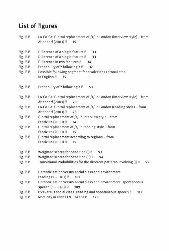
List of figuresFig. 1.1 Lo-Co-Ca: Glottal replacement of /t/ in London (interview style) – from
Altendorf (2003)| 19
Fig. 2.1 Difference of a single feature| 33Fig. 2.2 Difference of a single feature| 33Fig. 2.3 Difference in two features| 34Fig. 2.4 Probability of Y following X| 37Fig. 2.5 Possible following segment for a voiceless coronal stop
in English| 39
Fig. 3.1 Probability of Y following X| 53
Fig. 5.1 Lo-Co-Ca: Glottal replacement of /t/ in London (interview style) – fromAltendorf (2003)| 73
Fig. 5.2 Lo-Co-Ca: Glottal replacement of /t/ in London (reading style) – fromAltendorf (2003)| 73
Fig. 5.3 Glottal replacement of /t/ in interview style – fromFabricius (2000)| 74
Fig. 5.4 Glottal replacement of /t/ in reading style – fromFabricius (2000)| 75
Fig. 5.5 Glottal replacement according to regions – fromFabricius (2000)| 75
Fig. 6.1 Weighted scores for condition (i)| 93Fig. 6.2 Weighted scores for condition (ii)| 94Fig. 6.3 Transitional Probabilities for the different patterns involving [j]| 99
Fig. 7.1 Derhoticisation versus social class and environment:reading (n = 1103)| 107
Fig. 7.2 Derhoticisation versus social class and environment: spontaneousspeech (n = 8170)| 109
Fig. 7.3 (rV) versus social class: reading and spontaneous speech| 113Fig. 7.4 Rhoticity in Fred ELN: Tokens| 123
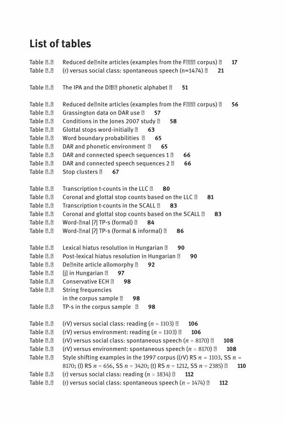
List of tablesTable 1.1 Reduced definite articles (examples from the Fred corpus)| 17Table 1.2 (r) versus social class: spontaneous speech (n=1474)| 21
Table 3.1 The IPA and the Disc phonetic alphabet| 51
Table 4.1 Reduced definite articles (examples from the Fred corpus)| 56Table 4.2 Grassington data on DAR use| 57Table 4.3 Conditions in the Jones 2007 study| 58Table 4.4 Glottal stops word-initially| 63Table 4.5 Word boundary probabilities | 65Table 4.6 DAR and phonetic environment | 65Table 4.7 DAR and connected speech sequences 1| 66Table 4.8 DAR and connected speech sequences 2| 66Table 4.9 Stop clusters| 67
Table 5.1 Transcription t-counts in the LLC| 80Table 5.2 Coronal and glottal stop counts based on the LLC| 81Table 5.3 Transcription t-counts in the SCALL| 83Table 5.4 Coronal and glottal stop counts based on the SCALL| 83Table 5.5 Word-final [ʔ] TP-s (formal)| 84Table 5.6 Word-final [ʔ] TP-s (formal & informal)| 86
Table 6.1 Lexical hiatus resolution in Hungarian| 90Table 6.2 Post-lexical hiatus resolution in Hungarian| 90Table 6.3 Definite article allomorphy| 92Table 6.4 [j] in Hungarian| 97Table 6.5 Conservative ECH| 98Table 6.6 String frequencies
in the corpus sample| 98Table 6.7 TP-s in the corpus sample | 98
Table 7.1 (rV) versus social class: reading (n = 1103)| 106Table 7.2 (rV) versus environment: reading (n = 1103)| 106Table 7.3 (rV) versus social class: spontaneous speech (n = 8170)| 108Table 7.4 (rV) versus environment: spontaneous speech (n = 8170)| 108Table 7.5 Style shifting examples in the 1997 corpus ((rV) RS n = 1103, SS n =
8170; (l) RS n = 656, SS n = 3420; (t) RS n = 1212, SS n = 2385)| 110Table 7.6 (r) versus social class: reading (n = 1834)| 112Table 7.7 (r) versus social class: spontaneous speech (n = 1474)| 112

xvi | List of tables
Table 7.8 Style shifting examples in the 1997 corpus: (r) (RS n = 1834, SS n = 1474)| 114
Table 7.9 Mean auditory rhoticity scores in Lawson et al. (2011)| 116Table 7.10 Rhoticity in Fred ELN: Tokens| 122Table 7.11 Rhoticity in Fred ELN: Ratios| 122Table 7.12 Coda [r] transitional probabilities in Fred East Lothian| 124Table 7.13 Coda [r] transitional probabilities in Fred East Lothian and Glasgow
working-class youth conversations data| 124Table 7.14 Variation in coda /r/ vocalisation| 125

1 PreliminariesSalientadjective1. Of material things: Standing above or beyond the general surface or outline; jutting out;
prominent among a number of objects.2. Of immaterial things, qualities, etc.: Standing out from the rest; prominent, conspicuous;
often in phr. salient point. Also Psychol. standing out or prominent in consciousness.The Oxford English Dictionary
This work is written with two aims. The first is to give a general discussion of saliencein sociolinguistics. This includes a focus on the use of the term in sociolinguistic discourse and in related sciences, especially cognitive psychology, since sociolinguistscan certainly benefit from the insights of researchers who approached salience from avery different angle. We will also look into the relevance of salience in sociolinguisticsfor theoretical linguistics as a whole.
The second aim is to put forward a particular method to operationalise saliencein sociolinguistics. This method will not be able to define salience in such a way as tocover all the uses of the term in sociolinguistics. It will, however, allow us to handle itas a theoretical construct – empirically testable and applicable to particular instancesof linguistic variation.
This work can be of interest to sociolinguists and students of linguistic variation,or indeed anyone who wants to become acquainted with salience as a theme in linguistics and sociolinguistics. It can also provide a starting point for researchers whohave an experimental approach to measuring and modelling linguistic variation.
In order to promote salience from being an umbrella term – applied by sociolinguists to a wide range of phenomena, including phonetic prominence, morphologicalcomplexity, or linguistic stereotypes – to the status of a rigid theoretical construct, wehave to tackle two questions. First, what types of linguistic variation are salient forthe language user? Second, how are these differences utilised by the language community? The first question requires us to talk in clear terms about linguistic variationand the way the language user relates to it. The second question connects to larger issues in linguistics, such as the mechanics of the propagation of linguistic change andthe architecture of linguisticmodelling.
After reviewing the use of the term salience in the sociolinguistic literature, thiswork makes a distinction between cognitive and social salience and offers a definitionfor both. Cognitive salience is the objective property of linguistic variation that makesit noticable to the speaker. Social salience is the whole bundle of the variation alongwith the attitudes, cultural stereotypes, and social values associated with it.
This is followed by case studies which show how cognitive salience can emergefrom the patterns of linguistic variation and how cognitive salience inputs socialsalience, which we observe through the attitudes displayed by the language commu

2 | 1 Preliminaries
nity. If a type of variation has cognitive salience, it can become socially salient. In thiscase, its objective qualities (standing out) are extended to carry a social meaning aswell.
Finally, Imakenote of the relevance of salience both to linguisticmodelling and totheories of language change. I will show that a clearly bounded notion of salience canplay a vital role both in the architecture and the theoretical foundations of languagemodels.
Sound patterns lie in the focus of this work. As we will see, the way I propose toformalise cognitive salience largely relies on evidence from the perception and acquisition of phonological patterns, and the case studies I discuss also involve variationat the sound level. While the theory of salience covered here can be extended to otherlevels of linguistic description, this work remains confined to sounds, especially sincethe phonological level dominates sociolinguistic discussions of salience.
This chapter establishes the setting of the rather complex task outlined above. Itgives a cursory introduction to the idea of salience in sociolinguistics and providesan outline for the argumentation to follow. We will have a look at linguistic variationand its consequences to social language use to see how the former is exploited – or,even more interestingly so, not exploited – by the latter. We will then go after the possible reasons why variation can be put to use by language users in different ways. Thisprobably has to do with both the properties of variation and the social dynamics ofthe language community in which variation takes place. After proposing a relationship between the properties of variation and its salience to the language users, thischapter gives a brief overview of the case studies supporting this proposition, alongwith the argumentation that is built on it: Section 1.1 introduces the main topic of thebook, Section 1.2 looks at how we will go after this problem, and Section 1.3 sums upthe chapter.
1.1 Salience and linguistic variationThis section introduces the notion of salience as a property of linguistic variation.First, salience is described in general terms, then I will discuss one particular operationalisation of the term, based on a cognitive premise.
1.1.1 Lexical reference and social indexation
Salience, as we will see, is usually regarded as a property of a speech difference. Systematically occurring speech differences come in two kinds: they can have lexical reference or a social index, or, indeed, both. Lexical reference is, quite simply, the difference in terms of the signified – elephant means something else than cake. Social

1.1 Salience and linguistic variation | 3
index here refers to a social meaning, a signal of the speaker’s background, identity,or intention, whichwe can treat as separate from a difference in the signified. Thoughthis split is, to some extent, artificial – apart from basic vocabulary, almost all wordshave at least some stylistic connotations, and some types of phonological variationare capable of neutralising lexical contrasts, so that pen sounds like pin, so lexicalreference and social index can never be completely separated – it still serves as theunderlying idea of the sociolinguistic variable. Weinreich et al. (1968), in an articlethat set the scene for a large bulk of variationist research to follow, define a linguistic variable as alternative ways of saying the same thing, adding that these ways havesocial significance.
This definition takes no note of words that mean different things and, instead,focusses on how variants of the same word that aremore or less synonymous are usedto express different social meanings.
A simple example to demonstrate lexical reference and social index comes fromthe Australian language Djirbal (Dixon, 1980). Djirbal has two vocabulary sets, onefor general use, and one to use in the presence of a particular kinship relation, whichDixon dubs mother-in-law. Though the mother-in-law set is more restricted, commonwords exist in two forms, one for each vocabulary set. Independent of the speech context, the Djirbal speaker has to use themother-in-law set in presence of such a kinshiprelation. What follows is that a Djirbal word has two functions: a meaning, that is, aparticular lexical reference, and a social index, namely, the presence versus absenceof the mother-in-law.
This is a categorical example: all words either belong to one set or the other, andspeakers are able to classify them upon inquiry (Silverstein, 2001/2009). (The waysocial index is used in this book is more generic than the term as defined by Silverstein. Here, it is essentially interpreted as a mark that the listeners use to associatethe speaker with a given social category, such as a social class or a coming from aparticular area.) We have reasons to believe, however, that social indexation is usually not that robust. While different words usually signify different concepts (exceptfor interjections, homonyms, etc.), not all dialectal differences index different groupalignments to the layperson. This is especially true for lower levels of linguistic description – language users are usually very much aware of particular words or intonation patterns other people use (though they are much worse in explicitly discussingthe latter than the former), but are much less attentive to phonetic differences. Thatis, there are consistent dialectal differences which are never recognised as such.
One can look at any known language for a fitting example. To take amore popularone, German has a Northern-Southern dialectal divide, which is reflected in quite anumber of variables. A difference speakers are usually aware of is that Southern German uses a definite article with proper names (at least in certain cases), so one cantalk about die Flora or der Peter, and so on. This is not present in Northern dialects –the same way it is not present in another Germanic language, English. At the sametime, Southern German dialects have a long [ɛː] where Northern ones have a long [eː],
4 | 1 Preliminaries
as in Schäfer ‘shepherd’ ([ˈʃeːfɐ]/[ˈʃɛːfɐ]). Speakers are much less likely to mention thisdifference when discussing the peculiarities of the Northern-Southern divide in Germany – they might not be able to recognise it as a difference at all.
The Southern German variant of the proper namewith the article is salient for theNorthern speaker. Northern speakers are much worse in telling the Southern variantof [ɛː] from their own variant of [eː], suggesting that the (e) variable is less salient forthem.
To recapitulate on all this once again, two dialects can differ in n variables, butonly a subset of these variables, k, is recognised by the speakers (not necessarily consciously). The way a speaker recognises a variable is that he or she recognises a variant – one that he or she would never use, or one that he or she would not use in thatparticular setting (and so on).
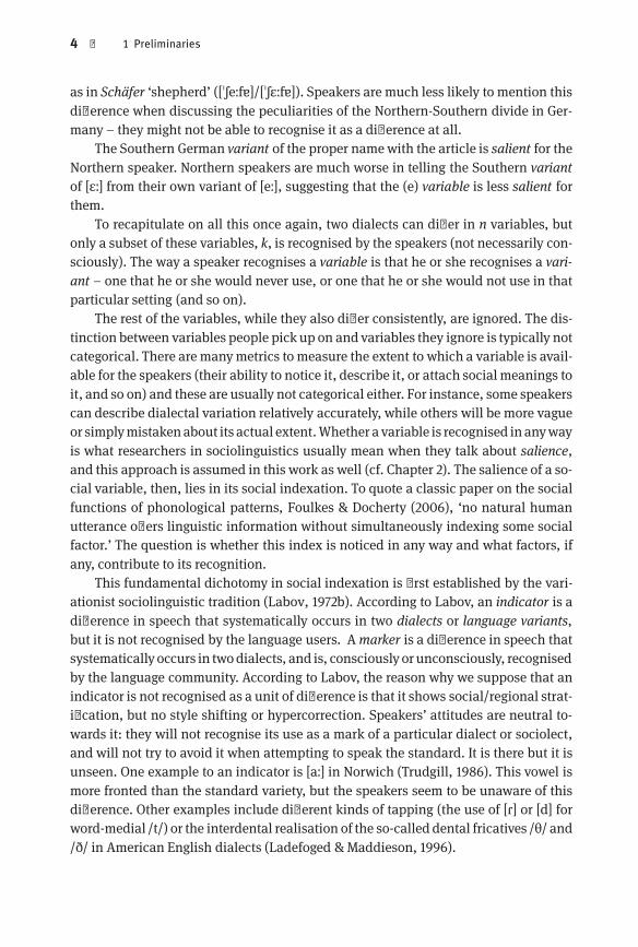
The rest of the variables, while they also differ consistently, are ignored. The distinction between variables people pick up on and variables they ignore is typically notcategorical. There are manymetrics to measure the extent to which a variable is available for the speakers (their ability to notice it, describe it, or attach social meanings toit, and so on) and these are usually not categorical either. For instance, some speakerscan describe dialectal variation relatively accurately, while others will be more vagueor simplymistakenabout its actual extent.Whether a variable is recognised inanywayis what researchers in sociolinguistics usually mean when they talk about salience,and this approach is assumed in this work as well (cf. Chapter 2). The salience of a social variable, then, lies in its social indexation. To quote a classic paper on the socialfunctions of phonological patterns, Foulkes & Docherty (2006), ‘no natural humanutterance offers linguistic information without simultaneously indexing some socialfactor.’ The question is whether this index is noticed in any way and what factors, ifany, contribute to its recognition.
This fundamental dichotomy in social indexation is first established by the variationist sociolinguistic tradition (Labov, 1972b). According to Labov, an indicator is adifference in speech that systematically occurs in two dialects or language variants,but it is not recognised by the language users. Amarker is a difference in speech thatsystematically occurs in twodialects, and is, consciously or unconsciously, recognisedby the language community. According to Labov, the reason why we suppose that anindicator is not recognised as a unit of difference is that it shows social/regional stratification, but no style shifting or hypercorrection. Speakers’ attitudes are neutral towards it: they will not recognise its use as a mark of a particular dialect or sociolect,and will not try to avoid it when attempting to speak the standard. It is there but it isunseen. One example to an indicator is [aː] in Norwich (Trudgill, 1986). This vowel ismore fronted than the standard variety, but the speakers seem to be unaware of thisdifference. Other examples include different kinds of tapping (the use of [ɾ] or [d] forword-medial /t/) or the interdental realisation of the so-called dental fricatives /θ/ and/ð/ in American English dialects (Ladefoged & Maddieson, 1996).
1.1 Salience and linguistic variation | 5
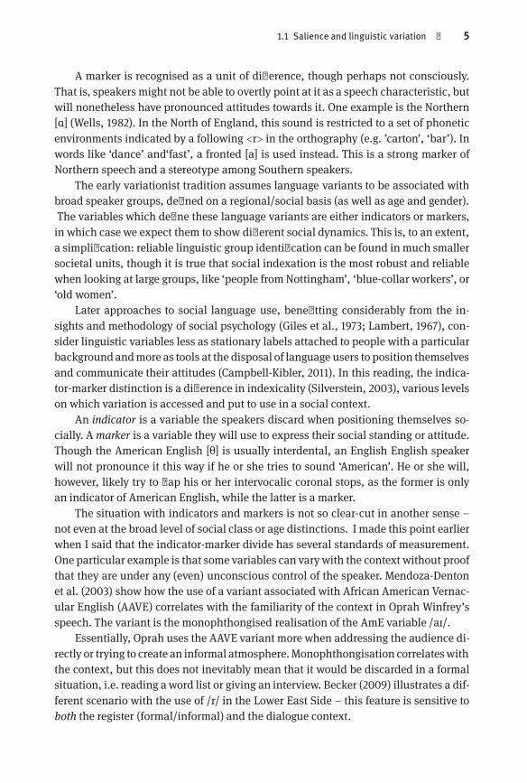
A marker is recognised as a unit of difference, though perhaps not consciously.That is, speakers might not be able to overtly point at it as a speech characteristic, butwill nonetheless have pronounced attitudes towards it. One example is the Northern[ɑ] (Wells, 1982). In the North of England, this sound is restricted to a set of phoneticenvironments indicated by a following <r> in the orthography (e.g. ’carton’, ‘bar’). Inwords like ‘dance’ and‘fast’, a fronted [a] is used instead. This is a strong marker ofNorthern speech and a stereotype among Southern speakers.
The early variationist tradition assumes language variants to be associated withbroad speaker groups, defined on a regional/social basis (as well as age and gender).The variables which define these language variants are either indicators or markers,in which case we expect them to show different social dynamics. This is, to an extent,a simplification: reliable linguistic group identification can be found inmuch smallersocietal units, though it is true that social indexation is the most robust and reliablewhen looking at large groups, like ‘people fromNottingham’, ‘blue-collar workers’, or‘old women’.
Later approaches to social language use, benefitting considerably from the insights and methodology of social psychology (Giles et al., 1973; Lambert, 1967), consider linguistic variables less as stationary labels attached to people with a particularbackgroundandmore as tools at the disposal of language users to position themselvesand communicate their attitudes (Campbell-Kibler, 2011). In this reading, the indicator-marker distinction is a difference in indexicality (Silverstein, 2003), various levelson which variation is accessed and put to use in a social context.
An indicator is a variable the speakers discard when positioning themselves socially. Amarker is a variable they will use to express their social standing or attitude.Though the American English [θ] is usually interdental, an English English speakerwill not pronounce it this way if he or she tries to sound ‘American’. He or she will,however, likely try to flap his or her intervocalic coronal stops, as the former is onlyan indicator of American English, while the latter is a marker.
The situation with indicators and markers is not so clear-cut in another sense –not even at the broad level of social class or age distinctions. I made this point earlierwhen I said that the indicator-marker divide has several standards of measurement.One particular example is that some variables can varywith the context without proofthat they are under any (even) unconscious control of the speaker. Mendoza-Dentonet al. (2003) show how the use of a variant associated with African American Vernacular English (AAVE) correlates with the familiarity of the context in Oprah Winfrey’sspeech. The variant is the monophthongised realisation of the AmE variable /aɪ/.
Essentially, Oprah uses the AAVE variant more when addressing the audience directly or trying to create an informal atmosphere.Monophthongisation correlateswiththe context, but this does not inevitably mean that it would be discarded in a formalsituation, i.e. reading aword list or giving an interview. Becker (2009) illustrates a different scenario with the use of /r/ in the Lower East Side – this feature is sensitive toboth the register (formal/informal) and the dialogue context.
6 | 1 Preliminaries
The problem with /r/ and /aɪ/ is that an indicator variable’s main characteristicis supposed to be that it does not carry social indexation and it is not available tothe speakers. In this case, such a variable is not expected to correlate with any factorbeyond the age, gender, and social background of the speaker.
Chopping up the linguistic variable set into indicators and markers is, then, dangerous in the sense that it implies a complete absence of gradience. It has to be notedthis early that the binary approach is only one of the possible operationalisations. AsPreston (1996) shows, linguistic awareness has many levels, very few categorical. Thelayperson’s grasp of dialect differences can differ in availability, accuracy, and detail:one can comment on an accent without being able to describe its characteristics, onecanpoint at a particular variant but define it inaccurately, and onemight not be awareof a recurring difference at all. What is more, a variable can have a large scope of realisations showing rampant variation and fine-tuned phonetic differences, making thelistener’s job evenmoredifficult. The concept ofmarker herewill refer to a variable thataffects speaker attitudes and behaviour. It shows style shifting and invokes positive ornegative attitudes, even if the language users are absolutely unable to pin it down. Theterm social saliencewill be used in a similarmanner: a variable has no social salienceif its realisations are stratified according to speaker background or context, but carryno social indexation.
Indicators and markers are discussed in Chapter 2, and we return to this issuein Chapters 8 and 9. This work, for the most part, can recur to the use of the markerconcept, as long as the theoretical background is always taken into consideration,along with the available evidence in each case we discuss.
Salience is, then, interpreted here as a property that allows a linguistic variable tobe amarker. In the case studies, attitude tests are used to determine whether it is usedin the speech community for indexing purposes. As the review of the literature on thisconceptwill show, this is a rather narrowdefinition–but a very goodone for a researchmethodology. To go back to the extremely simplified German example above, the useof definite articleswith proper names is then amarker of the difference betweenNorthern and Southern dialects, whereas the realisation of the mid-front unrounded vowel([eː]/[ɛː]) is not. Whether this is the case we can test by looking at listener attitudes tospeaker voices that show variation of either of these variables.
We expect that if we ask people whether they hear any differences between voicesusing variants of both variables, they will recognise and comment on definite articles much more successfully. (Of course, the situation is easier when a variable is anextremely strong stereotype, as is the use of definite articleswith proper names in German, witnessed by overt social commentary.)
Establishing that sociolinguistic salience is a property of a linguistic variableleads to two further questions. The first is whether the salience of a variable can belinked to a structural or an extra-linguistic property which would allow us to predictwhether a particular variable will be used for social indexation. This is one of the
1.1 Salience and linguistic variation | 7
main aims of this book, and it is discussed in some detail in the next section. Thesecond question concerns the theoretical relevance of salient variables.
Sociolinguistic salience as a theoretical building block of language models is relevant in two particular ways. First, an operationalisation of salience allows a modelto separate salient and non-salient (or less salient) variables in an empirical way. Second, if sociolinguistic salience is a property of variables, we expect it to play a role inthe propagation of language change, that is, the way novel variants are transmitted inthe speaker community .
Sorting out variables according to the extent to which they are subject to speakerawareness (or are available to carry social indexation) is a central issue in modellingthe individual’s linguistic competence. As discussed in the next section, early variationist research had a relatively straightforward way of separating indicators frommarkers, based on the stage of language change and, alongwith it, the extent of variation present in the speech community. Themore people use a variant, themore salientvariation becomes.
If we argue that salience is not a deterministic function of the stage of languagechange, and not just a word that sociolinguists use when they find a variable conspicuous either, wehave to find an independentmeasure to account for this property. Sucha measure is important because it allows us to separate types of structured phoneticvariation which carry social indexation from types that do not – with some empiricalgrounding at least. Salience and language modelling is one of the questions exploredin detail in the second half of this book, and the subject of Chapter 8.
Another relevant issue is whether salience – here loosely interpreted as the extent to which the variable carries social indexation – is involved in the modellingof language change at all. An ongoing debate in sociolinguistics, surveyed in Chapter 9, focusses on whether personal preferences should be involved in adopting newlinguistic variants, that is, whether the propagation of a variant is dependent on theconnotations it carries. Simply put, this question is quite close to the issue of the indicator-marker continuum introduced above. In a model that regards all variables asindicators, their propagation entirely depends on the number and participants of interactions in the speaker community (irrespective of whether variables are subject tospeaker awareness in any other way not taken into consideration by the model). Ifsalience plays a role in the adoption of new variants, we expect that it affects the waychange is propagated. Non-salient variants will then spread dependent only on thefrequency of interactions, while salient ones will be subject to speaker preferences –their use might be advocated or avoided, depending on the social indices they carry.
Consequently, salience, however we define it, is relevant to the question of thepropagation of a sound change, though not to its actuation. This problem is exploredin detail in Chapter 9.
There is a lot of talk on social indexation throughout this book. While the termowes much to Silverstein (2003), in whose work it partly originates, it is used moreloosely here. In this work, social indexation refers to any sort of social information
8 | 1 Preliminaries
attached to structured variation in the language community, whether it be a grouplabel, a set of attitudes, or a general stigma or prestige. Treating the social indexationof a linguistic variable this way, along with the focus on individual variables, gives upmost of the insights of second and third wave sociolinguistics (cf. Chapter 9). This is,however, done in such a way that these insights are not lost and, at the same time,the focus is kept on linguistic variation, considering the social reflexes in the moststreamlined way possible.
1.1.2 Concepts and notations
Throughout this book, oblique parenthesising marks an abstract segment type andsimpleparentheses a sociolinguistic variable. Squarebrackets refer to aparticular segmental realisation and chevrons to an orthographic form of either an abstract type ora variable. For example, in Chapter 7, I talk about /r/,which is a contrastive segment inScottish English. It can be realised in variousways, such as [r], a central approximant,[ʁ], a retroflex approximant, or [ɾ], an alveolar tap.
If we posit a variable on /r/ realisation, we can call it (r). We can then posit all theabove realisations as variants of (r), alongwith the vocalised, deleted variant [V]word-finally. (Note that this one variant is more abstract and not directly interpretable.) Wecan posit another variant, (rV), which only includes word-final variation in /r/ realisation, andwe can distinguish other realisation variants for it in the vocalised variantgroup. Needless to say, all these units will be written as <r>, because English orthography is insensitive to the subtleties of rhotic variation. Finally, small caps are usedto refer to lexical sets (Wells, 1982).
The system of notations acknowledges three broad types of linguistic variation: alanguage variety differs from other varieties in certain ways. These differences can beseen as linguistic variables –multiple ways of saying the same thing. The realisationsof a variable are its variants. A variable, then, is an abstract unit with social indicesand even strong stereotypes attached to it. A variant is a concrete unit, which can havedistributions in the speech stream or in a corpus. The notations express no commitments on the ontological status of these segments, but it is important to keep themapart.
1.1.3 Salience as low probability
As noted in Section 1.1.1, the salience of a variable in the speech community can be determined by independent measures. The best tools are attitude studies, which clearlyshow whether listeners associate the presence versus absence of a variant with a particular geographical location or social stratum. Style shifting, hypercorrection, and, ofcourse, non-linguist comments all strongly suggest that a particular variable is a soci
1.1 Salience and linguistic variation | 9
olinguistic marker. A questionwhich usually receives less attention is which variablesbecome social markers.
Originally, Labov (1972b) proposes that all variables start their life spans as indicators, and later, as the particular language change gains momentum, propellingthem further, they becomemarkers for the language users. In subsequentwork, Labov(2001) discards this hypothesis, noticing that some variables never reach marker status. If we are to maintain that salience is an objective property of a linguistic variable,we need to find a basis on which we can ascertain whether a variable is salient.
This is one of the most important questions of this book. Is there a reason that,for example, the place of articulation of English fricatives receives less attention thanthe manner of articulation of English stops? Is it just an accidental consequence ofthe social dynamics of English speakers, is it, as Labov once suggested, an outcomeof language change, or does variation have defining characteristics that determinewhether language users become aware of it?
As we will see in Chapter 2, an intuitive way to ground salience in sociolinguistics is to look at the way the term is used elsewhere. Salience, as a concept, is usedstraightforwardly in the cognitive sciences, as in discussions of visual perception, oreven in specific, practical sub-domains, such as advertising (Itti, 2005). It is usuallyseen as a bottom-up notion, connected to a principal part of human perception, surprise. An entity is surprising if its presence has a high information value compared toits surroundings – that is, when its presence is not probable, but unexpected.
The hypothesis assumed here is that salience in sociolinguistics also derives (atleast partly) from low probability of occurrence. An unexpected, surprising variantcan be utilised to index social differences – though not necessarily. The merits of thishypothesis are that it can be operationalised easily and that it provides an empiricalfoundation for the concept of salience in sociolinguistics. It also has its limitations.For example, ongoing, socially stratified vowel shifts have a strong social significance,but this does not trivially follow from any difference in distributions – vowel qualitieschange, but quantities stay the same. I will return to the issue in Chapter 10.
One example of the correlation between low probability and salience is the process of definite article reduction, which has been described as occurring in the Northof England (Lodge, 2010; Jones, 1999). To put it very simply, the process entails thevariable reduction of the definite article into a glottal stop. This reduction pattern isconfined to the North of England and it is not particularly frequent, most surveys giving figures of ten to fourteen per cent of all definite articles reduced. The pattern varieswith age and gender, and shows style shifting. What is more, it is an overt stereotypeof Northern speech, making it an exemplary salient marker.
If we look at the distribution of glottal stops in the norm dialect (such as Northernvarieties of RP or indeed any English English dialect without definite article reduction) we see that glottal stops havemuch larger transitional probabilities in particularpositions in the reducing dialects vis à vis the standard. For example, we find a glottalstop followedbya stressed vowelmuch less often in the standard than ina reducingdi
10 | 1 Preliminaries
alect (where definite articles standing before vowel-initial words stand a chance to bereduced). What follows is that the reduced articles are in conspicuous positions whencompared to their distributions in the standard dialect, which leads to their salience.
While article reduction is relatively frequent as a morphological variable (definite articles being one of the most frequent words in corpora), it is nowhere near therobustness of phonological variables, rendering its status as a social marker not entirely intuitive. A surprisal-based argument explains why reduced articles stand outeven when compared to other phonological patterns.
This was a simplified discussion, and I return to definite article reduction in Chapter 4. The principal reason of bringing it up here is to illustrate the concept of salienceas as a function of low probability. It serves as a good illustration of the kind of patternwhich is easily testable under our assumptions. It also helps to clarify the relationshipof the concept surprising, salient, andmarker. The variable’s salience follows from thevariants’ low transitional probability or surprisal, which, in this case, is clearly measurable. The property of salience is essential for the variable to become amarker, thatis, to acquire social indexation.
In this interpretation, salience is a property of a sociolinguistic variable, emergentduring language use. It stems from the perceived difference between the transitionalprobability patterns of the realisation of the variable in one dialect as opposed to others. This difference is the source of the variable’s surprisal,which leads to its cognitiveand sociolinguistic salience. In a simplified scenario, the surprisal of a variable comesinto view during a series of interactions between speakers of different dialects. The listener, who has a different dialect and therefore a different distribution of the variable,picks up on this difference when listening to the speaker. This is the source of the cognitive salience of the variable. If the variable is then used to carry social indexation,wecan call it socially salient. This is obviously very much a black and white way of looking at the problem, and still does not trivially explain how the surprisal of a variantcan be calculated – and the way surprisal is measured is crucial to the argumentationin this work. I talk about modelling the salience of a variable at length in Chapter 3.
As stated above, the locus of discussion throughout this work is phonology, onlypartly becausemost of the literature on salience explores this domain. Phonology alsooffers clearcut ways of abstraction and segmentation, allowing us to make comparisons of the above kind relatively easily. Last but not least, phonological variation isa central level of socially relevant linguistic variation. This is no surprise, as slightchanges in pronunciation are excellent tools to mark social indexation while preserving distinctions in semantic reference. (That is, it is easy to say a word in two slightlydifferent ways where the difference is big enough to be noticed but small enough toleave lexical referents unaffected.)
The programme developed in this work offers an operationalisation of saliencebased on cognitive grounds and a corpus-linguistic methodology. Through a seriesof case studies, I show how this operationalisation can be used in various ways as a
1.2 Structure of the book | 11
valid source of sociolinguistic salience. After the case studies, I go on to discuss therelevance of a testable notion of salience to linguistic modelling.
This programme makes a distinction between cognitive and sociolinguistic sa-lience. A variable attains cognitive salience if its realisations have a high enough surprisal value when compared to each other. This is argued to be the case above withdefinite article reduction – the dialect variants with reduced allomorphs of the articlehave different distributions of the realisation of the variable, such as the glottal stop,when compared to the dialect variants with the regular allomorphs. A variable thathas cognitive salience can carry social indexation, in which case it becomes sociallysalient for the speaker community. Socially more salient variables (both cognitive andsocial salience are taken to be gradient attributes) behave differently in social language use – they might be adopted or avoided more readily, for instance.
1.2 Structure of the book
1.2.1 Methodology
After establishing the sociolinguistic and phonetic-phonological correlates of sa-lience, the procedure is the following: we take a look at different phonological variables that arguably have the former and see if they also share the latter. That is, for avariable V, we have evidence that V is used for indexation, and are curious whetherthere is a significant case of jutting out in V’s variants’ transitional probabilities (inan inter-dialectal comparison).
This is based on the assumption that a variable has to be surprising in order to besocially salient, but not all surprising variables will be necessarily socially salient.
The reasons for this assumption are twofold. First, low probability is not the solefactor in salience. A variable’s promotion to marker status depends on its position inthe language community and the attitudes present in this community in general. Thesocial evaluation of a variable (or lack thereof) is necessarily entangled with externalfactors such as the structure of the language community and the thorough consideration of these factors in each case is beyond our scope. In the cases under scrutinywe are safe to say that cognitively salient variables took up social indexation, and thenon-linguistic forces behind them are more or less taken for granted. Second, a lowprobability variant can be so unlikely to occur that it does not reach the threshold ofconsciousness at all, in which case it is ignored completely – low probability of occurrence needs to be paired up with a certain amount of robustness in the speech signal.Putting it differently, a sequence has to be frequent enough for people to notice howrare it is.
With this in mind, research is exclusively concentrated on socially salient phonological variables, mostly from the segmental domain. Constructing a line of argumen

12 | 1 Preliminaries
tation in favour of the causation between low probability of occurrence and socialsalience then proceeds as follows.1. Identification of a variable: A dialectal variable is picked and defined narrowly.
The latter step is quite useful inasmuch as the use of different terms in the literature can be rather fuzzy. For instance, glottalisation might refer to the glottalreinforcement of fortis stops attested in dialects in England (as in [khæʔpthən]ʻcaptain’), the glottal replacement of /t/ in some subsets of these dialects (as in[bæʔmæn] ‘Batman’), or even solely to the glottal replacement of /t/ in a numberof very specific environments, such as word-medially before a vowel ([lɛʔə] ‘letter’) or before a syllabic sonorant ([bʌʔl
ˈ] ‘bottle’). Similarly, the term rhotic comes
up both in the sense of a rhotic/non-rhotic distinction (as in Scottish Standard English versus Southern English English) or speaking of rhoticised vowels in American English, and so on.
2. Background check: The literature on the particular variable is partly surveyed.This is not only crucial to the understanding of themechanics of the feature itself,but also necessary to confirm its salience. A marker shows style shifting and hypercorrection and itmight be the subject of overt commentary and ridicule, whichmakes it even easier to argue that it carries social indexation. Fundamentally, itshould trigger changes in attitude, if it is – even covertly – associated with a particular region or social register. These attitudes can be caught in the act by sociolinguistic interviews and attitude studies (cf. e.g. Labov et al. (2006)).
3. Choice of corpora: In order to find out about difference in transitional probabilities between the dialect featuring the marker and the respective standard, onemust find corpora of both to work with. As written registers force standardisation,spoken material is preferred. In case the spoken material is only available in atranscribed form, but without recordings, the ratios of the marker can be extrapolated using the transcription and relevant studies on the extent of the marker’suse. One corpus to use when working on variation in England is the Fred corpus(Kortmann et al., 2005), a collection of sociolinguistic interviews covering all major English dialect areas. Themainmerit of this corpus is that data were collectedconsistently and in a similar fashion from all major dialect areas, allowing for astraightforward comparison. It contains recordings and transcriptions, which renders it even more suitable for any investigation of phonological variation. In casemore data are needed from a particular dialect area, auxiliary corpora can be putto use – to give two examples, Cheshire et al. (2008) have a large corpus of adolescent speech in London, and there are similar projects for other dialect areas,like the Newcastle Electronic Corpus of Tyneside English (Allen et al., 2007) forNewcastle and the Tyneside.
4. Computing probabilities: Differences in transitional probabilities for the dialectwith the vernacular variant versus a standard or norm dialect (with the standardvariant) are calculated. In the case of Northern English, for instance, the looming presence of the Received Pronunciation (RP) as the national standard gives
1.2 Structure of the book | 13
us enough reason to compare a dialectal variation pattern with it. The internalspeaker norm can be, however, inferred in most cases from attitude studies andthe sociolinguisticmakeupof thearea. Thefinal result is amodel of thedialect anda model of the norm, but these models are reliable enough for us to make meaningful statements about them. If there is a high enough difference in probabilitiesbetween the dialect and the norm, we are safe to say that this gives the variableits unexpected, surprising quality, and, indirectly, its salience. Salience does notnecessarily emerge in a standard-vernacular relationship, but our examples willmostly belong to this common type.
Apart from relying on the literature of the different variables in particular and ofsalience and psycholinguistics in general, this research method employs two sets oftools: corpora and computing transitional probabilities. The choice of corpora has tobe carefully made, and backed up with independent studies on the reliability of thecorpus, as well as the behaviour of the feature in the dialect. The use of transitionalprobabilities in linguistics has a long tradition dating back to Harris (1955) and thestructuralists, but since the methodology used in this work is novel in a number of respects, it warrants an extent of caution. Both the question of corpora and themethodsof computation are elaborated in more detail later.
Two premises have to be spelt out in connection with this methodology, both connected to the fact that, in this programme, corpora are taken to be representative ofdialects in contact. First, even a comparison of spoken corpora of particular dialectsdoes not directly match the interaction of the speakers of these dialects, or even theimplicit knowledge that a speaker of one dialect has about another dialect. Since, especially in the case of phonological variables, the size of the corpora makes up inredundancy for this level of abstraction, and since a direct model of speaker interaction is much more difficult to model (and more prone to error), corpora are used inlieu. Second, if we compare local dialects with a supra-local dialect or a standard, wehave to be careful in our choiceswhen defining the latter. For instance, above I arguedthat Northern English local dialects can be compared to RP as the supra-local dialectof Britain, but this is not the case, at least not trivially so. In order to have a meaningful comparison of dialect corpora, the choice of corpora has to be grounded in ourknowledge of the social dynamics of language use in the region we focus on.
1.2.2 Chapter structure
This work consists of three parts. The first part, the introduction, considers the notionof sociolinguistic salience as used in the literature, and proposes an operationalisation of this concept. The second part contains a series of case studies in which themethod of operationalising salience is used, building on various types of available

14 | 1 Preliminaries
data. The third part argues for the relevance of salience to linguistic theory, using theexample of models of language competence and language change.
Chapter 2, a review of the literature on salience, follows this introductory chapter.I have a brief look into how the concept is used in the cognitive sciences, especiallywith respect to visual cognition. The similarities and differences between cognitivesalience and the way sociolinguistic salience are interpreted are going to provide auseful starting point for any further discussion.
The more substantial part of the chapter deals with salience in sociolinguistics.As I wrote above, my definition of the term is rather narrow. Sociolinguists regard theconcept of salience as having a wide range of properties, frommerely equating it withhigh token frequency to attributing an extra-linguistic property to it. A partial surveyof the available studies working with this concept provides a feasible background forthe use of the term here. It is also a starting point for our discussion – no matter hownarrow and exclusive a definition we give to sociolinguistic salience, this definitionhas to be put in the context of previous studies which referred to the concept.
We also have to be careful when taking into consideration all the possible sourcesof sociolinguistic salience. For instance, salience should not be equated with token frequency. Another potential hazard is basing its definition on other, similarlyvaguely-defined concepts, such as markedness. Markedness is, in principle, the theory of sound segment complexity. According to markedness theory, some sounds aremore complex than others, and this shows in their phonetic properties, acquisition,and behaviour in sound changes. One could then simply say that the salience of asound segment increases proportionally as a function of its markedness. Markednesstheory, however, has a huge amount of problems on its own (Harris, 2005; Ohala,1971; Blevins, 2004), and its relationship to salience is vague to say the least, despiteattempts to relate the two with each other (cf. Chapter 2).
To cite one issue, a frequent example of markedness – as a principle operatingin language – is the case of consonants with two places of articulation. You wouldnot expect to find a language with a labio-velar stop [⁀kp] but without a labial and avelar stop. Similarly, one would think that a labio-velar stop will be more salient forthe listeners than a labial or a velar stop on its own. That might very well be the case,but this system easily breaks downwithmore complicated examples. For instance, theSouthern English English /t/ has two usual realisations, a slightly affricated one ([ts])before (stressed) vowels and a debuccalised one ([ʔ]) everywhere else. The affricatedrealisation is far more complex and should be deemed more marked in any case (asthe [ʔ] results from lenition) Yet, listeners seem to be sensitive to the glottal stop, ifanything, and, on the whole, ignore extents of affrication, which should be at oddswith a markedness-based account. Similar examples are not hard to come by.
Finally, Chapter 2 elaborates on a theory of salience as low probability of occurrence. This starts with a review of the literature on transitional probabilities. If I amto argue that probabilities extracted from the speech signal are largely to blame forthe selection of markers, I have to prove that listeners are sensitive to this type of in

1.2 Structure of the book | 15
formation. This is far from self-evident: Zeilig Harris originally proposed reliance ontransitional probabilities as a method for the field linguist.
His idea was that since word-medial segmental sequences are subject to phonotactic restrictions, while word-internal ones are not, the transitional probability of asegment X following Y(X∣Y) will be higher word-medially. Consequently, low transitional probabilities suggest word boundaries. For example, English [t] can be onlyfollowedby liquids andglides in anonset, but bypractically anything if it stands at theend of the word. If the field linguist is unable to segment an unknown language, theycan use transitional probabilities between the segments to determine word boundaries.
The distribution of sounds in the signal (or, as we see it, in a larger corpus) belongs crucially to the parole, as it follows entirely from the phoneme inventory andmorpheme structure constraints of the language, as well as from the way words areconcatenated – so syntax and word order also play a minor role.
The structuralist assumption, then, is that the structure of the langue affects theshape of the parole, and the observant field linguist can exploit this to arrive at generalisations on the former. This path is shut off for the language user, however, as parolehas noway to have an effect on langue directly. Consequently, since probabilities of occurrence are only available from the latter, they do not count as linguistic information.The psycholinguistic tradition, however, clearly supports that listeners are sensitiveto transitional probabilities from a very early age, as they provide a vital cue for wordsegmentation (precisely the task Harris had in mind). If we look at cases where theonly reliable cues of word segmentation are transitional probabilities, and word segmentation is better than chance-level (Saffran et al., 1996b), we have to accept thatlisteners somehow keep count of this part of performance. Psycholinguistic researchprovides the necessary empirical grounds for invoking sensitivity to distributions insociolinguistics proper.
Chapter 3 is a detailed walkthrough of modelling dialects with the purpose of discerning variant transitional probabilities in them. The aim of the chapter is to makethe reader familiar with the method advocated in this work of building dialect modelsbased on studies and corpora, and to make this method transparent and repeatable.
After the theory is established, it is tested in the case studieswhich follow in chapters 4–7. As stated before, the case studies provide phenomena which are certainly regarded as salient by the language community, and this salience can be aligned withtheir low probability of occurrence in a cross-dialectal setting. Essentially, the twofactors are established independently. It is first proved that the pattern in questionbehaves like amarker, and then, that it has a low probability of occurrence in comparisonwith a norm dialect. The nature of the norm dialect is carefully discussed in all ofthe cases, as this answers the central question of salience: to whom is a dialectal feature salient – the speakers who use the salient, non-standard variant, speakers of thestandard, or both? In the usual case, all members of the language community have anotion of the standard, and, consequently, are able to identify instances of structured
16 | 1 Preliminaries
variation that differ from it saliently. The case studies are drawn from the literature onEnglish variation. Due to the extensive work on English dialects, they provide a widepool of data and analysis which both can be relied on in these investigations.
The case studies all differ in their methodology and results. They illustrate atrade-off between robustness and abstraction when using corpora in the study ofsalience in sociolinguistics, where the use of spoken corpora allows an argumentation that is more directly related to the data, while the use of larger, written corporaallows for more robust generalisations, albeit achieved at the cost of higher abstraction.
In chapters 8-9, a general discussion follows the case studies, where, once again, Idraw conclusions, and consider themerits and faults of the theory. Themerits are that,ideally, it provides an empirically falsifiable structural ground for salience, one thatit hitherto lacked. Furthermore, it might provide a new insight on the forces behindphonological patterning. The faults are mostly that it is limited in certain ways, andnot universally applicable to all known dialectal variables. The final chapter providesbrief conclusions.
Chapter 8 puts forward a further argument to support an approach to socialsalience based on relative frequencies, namely, that such an approach can be directlyaccommodated into models of linguistic variationwhile considerably improving theirdescriptive adequacy.
Chapter 9 also puts the theory of salience into a broader context, and looks at itsimplications for a theory of language change. Chapter 10, while providing the general conclusions, also returns to an issue left in Chapter 2. Not mistakenly identifyingsalience with something else, like markedness, is a good start, but we have to takeheed not to draw inviting parallels between salience and any phonological or socialaspect either.
For example, one could argue that the phonological patterns that typically become salient are the categorical ones, where the distinction is coded at some higherlevel, such as front/back or lax-tense. One could also find evidence that the typicallysalient patterns are the low level, gradient ones, including distinction such as vowelheight or consonant VOT. We will see that salience cannot be associated with anylarger level of description, however.
1.2.3 The case studies
1.2.3.1 Definite article reduction
Definite article reduction is a dialectal phenomenon attested in the North of England,predominantly in Yorkshire and Lancashire. It is a salient feature par excellence, as ithas been one of the strongest stereotypes associated with Northern speech since theWuthering Heights (Jones, 2007; Lodge, 2010). This might be surprising given the fact

1.2 Structure of the book | 17
Table 1.1. Reduced definite articles (examples from the Fred corpus)
the day [ʔdeɪ] the inn [ʔin]the pub [ʔpʊb] the apple [ʔæpl
ˈ]
the cooker [ʔkʊkə] the order [ʔodə]
that the reduced article is relatively rare. Most surveys on the subject put reduced realisations between 10 and 14 per cent of all articles. Nonetheless, it is a viable pattern,which is further corroborated by the increase in its use in the city of York (Tagliamonte& Roeder, 2009). It seems that younger York males use the reduced variant more extensively in order to mark their social and regional identity.
The basic pattern of the reduction is that the definite article can be realised asa glottal stop before consonants and vowels, or, to a lesser extent, a voiceless dentalfricativebefore vowels (Table 1.1, cited fromChapter 4). This is a simplifieddescription,but, to a large, extent, accurate. It is also important to note that the reduced variant,despite the name, cannot be directly linked to the standard article. Neither its historynor its phonetic properties suggest that it is a phonetically reduced variant. Rather, itis a full-fledged allomorph in itself.What is curious about this dialectal pattern is that its frequency does not provide a sufficient explanation for its salience. It is true that definite articles are among the mostfrequentwords inEnglish, so even tenper cent of these articles is quite anumber. Froma phonological perspective, however, this number is less convincing. Since phonological features are more robustly present in the speech signal, the reduced article is inno way excessively frequent in this context. The phonetic properties of the reducedarticle are no cause for concern, either. The glottal stop, the overwhelmingly commonrealisation of this dialectal feature, is a common feature of dialects in England, resulting from the variable reduction of the fortis stops, typically [t], in word-final and pre-consonantal environments.
The theory of salience proposed in this work, however, explicitly states that theinteresting part is not the what, but the where. The glottal stop realisations of thereduced article can show up in environments where one would not commonly expecta glottal stop otherwise, such as between vowels, or before a stressed vowel. Whileit is possible for glottal stops to occur in these positions even without definite articlereduction, it is not usual, and this is precisely what makes these articles salient.
As the case study shows, the transitional probability of definite articles realisedas glottal stops is always smaller than the same probability of ‘regular’ glottal stops ina dialect lacking this feature. This means that both speakers of the standard (indeed,any standard, as long as this feature is absent from it) and dialectal speakers aware ofa standard will regard this feature as extremely salient.
This feature is very salient, goes the argument, no wonder it is used as a marker,for instance in the city of York. The young York males can rely on definite article re

18 | 1 Preliminaries
duction to support their Northern identity, since it is quite visible in the sense that itcan be picked up easily. Since we have no other reasons for the feature’s salience, theprobability-based explanation sounds quite plausible.
1.2.3.2 Southern English /t/ glottalisation
Glottalisation, or the realisation of /t/ as a glottal stop, is a classic feature of SouthernEnglish. Itwas first noticed in London in the early twentieth century. Daniel Jones himself first mentions the debuccalisation of /t/ in a footnote in 1923 (Jones & Trofimov,1923), postponing a sizeable discussion to 1932. Jones and his circle gradually recognised /t/ debuccalisation first before a syllabic nasal, including environments beforeliquids and glides later. During the course of the century, glottalisation gained morehold, appearing before all consonantsword-medially, before consonantsword-finally,and later before vowels in the same position. The present patterns include variableglottalisation in all positions, except word-initially and before stressed vowels. (Formore details on the spreading of the pattern, cf. Hudson & Holloway 1977; Williams &Kerswill 1999.)
One survey exploring the distributions of /t/ glottalisation in detail is Altendorf(2003), who distinguishes three social strata (working class, middle class, upper-middle class), two registers (written and spoken) and six environments, (word-mediallybefore a consonant, word-finally before a consonant, utterance-finally, word-mediallybefore a vowel, before a syllabic consonant, and word-medially before an unstressedvowel).
Her main findings are that in the spoken register, and especially in working classuse, [ʔ] almost categorically replaced [t]. Themiddle class and uppermiddle class use,however, shows that it is quite strongly avoided in formal registers and in certain environments, most notably before a vowel – both word-finally and word-medially (Figure 1.1).
The avoidance of /t/ glottalisation before a vowel canbepaired upwith an attitudetest performed by Fabricius (2000). She found that her upper-middle class speakershave significantly different judgements onword-final pre-consonantal andpre-vocalicglottalisation – simply put, while word-final pre-consonantal glottalisation (as in ‘getby’ [ɡɛʔbaɪ]) is more acceptable, word-final pre-vocalic glottalisation (as in ‘get away’[ɡɛʔəweɪ]), according to the listeners, should be avoided. This attitude study, alongwith the avoidance of /t/ glottalisation in precisely this environment, strongly suggestthat pre-vocalic /t/ glottalisation is a low prestige marker. (This is corroborated byRosewarne (1984), who explicitly mentions word-medial pre-vocalic /t/ glottalisation,the ‘letter’ or ‘butter’ type, as a social stereotype.)
Pronounced listener attitudes are not the sole proofs of salience. To give a moreloosely related example, Foulkes & Docherty (2006) show that in their Newcastle dataon child directed speech, mothers use more glottal stops when talking to their sons

1.2 Structure of the book | 19
C #C ## #V L/N V_V
Environments
Ratio
0.0
0.2
0.4
0.6
0.8
1.0
Fig. 1.1. Lo-Co-Ca: Glottal replacement of /t/ in London (interview style) – from Altendorf (2003)
than when talking to their daughters (it has to be noted, however, that the variantthey investigated is a different type of a glottal stricture very much stereotypical ofGeordie). Men use more glottal stops than women in Newcastle, which is in line withthe general observation that women are usually closer to the norm (Labov, 1994). Thefact that this is projected to child directed speech strongly suggests that glottalisationis a salient feature in this dialect, as mothers – implicitly – try to meet the standardthat women should speak more ‘properly’ to their female children.
Again, if we look at the distribution of the glottal stops, we can find good reasons for the salience of the pre-vocalic pattern. In an ‘untainted’ upper middle-classdialect, which allows no glottalisation before a vowel, any glottal stop in this environment is highly unexpected, as they have a transitional probability which is practicallyzero. Even though such a dialect probably never existed, the fact remains, that if pre-vocalic glottalisation is relatively new, its transitional probability will be extremelylow. It is important to note at this point that this is not the glottal stop’s fault per se.There are no pronounced attitudes agains glottalisation pre-consonantally, where it isa phonetically natural phenomenon, and where it probably has been occurring for awhile now. In sum, this feature developed salience as it spread to a new environment.
The salience of glottal stops that precede vowels as opposed to the ‘commonplace’quality of glottal stops preceding consonants is another curious case of phonologisation pairing up with social indexation. As long as glottalisation is restricted to positions where it is phonetically motivated, it stays below the threshold of listener sen
20 | 1 Preliminaries
sitivity to sociolinguistic variables. As soon as the pattern is generalised to new environments, where its appearance is phonetically ungrounded, it becomes perceptibleand prone to incite listener judgements. The reason, however, is not phonologisationitself, but the phonetic sequences created as its result.
1.2.3.3 Hungarian hiatus resolution
The aimof the only non-English example is to illustrate the general applicability of thetheory of salienceproposed in thiswork.Hungarianhiatus resolution is another example of a partly phonologised pattern. Alongside lexical hiatus resolution we also findpost-lexical, phonetic hiatus filling with the high/mid unrounded vowels [i] and [e].In innovative language variants, this pattern is extended to the open mid unroundedvowel [ɛ]. Hiatus resolution – always involving the glide [j] – is obligatory and unnoticed with [i]. It is variable to a certain extent with [e], but this is not subject to anylinguistic awareness either. It is, however, salient, and strongly stigmatised in vowelclusters involving [ɛ] (but not [i] or [e]).
The chapter consists of two major parts. The first part is the discussion of a perception experiment aimed at establishing the salience of hiatus resolution with [ɛ]as opposed to the other patterns. Results show that listeners are more judgementalwhen it comes the absence or presence of hiatus-filling [j] in vowel clusters involving[ɛ], which clear effect is notably absent with the other front unrounded vowels. Thesecond part of the chapter is a corpus study which models the conservative standarddialect without the salient hiatus resolution pattern in order to show that the difference in salience is supported by a relative frequency difference in the Hungarian caseas well. That is, while clusters of [ɛ] plus [j] are allowed in Hungarian, they are vastlyoutnumbered by sequences of [i] plus [j], which explains while the occurrence of theformer is noted by listeners, while the occurrence of the latter is not.
1.2.3.4 Rhoticity in Scotland
The distribution of /r/ is one of the most widely researched sociolinguistic features.Labov (1966/2006), in a groundbreaking study, reports on the social stratification ofrhoticity in New York City. His general results are that the absence of [r] in coda position is generally associated with lower social prestige and informal registers.
Labov argues that rhoticity is a marker of New York City speech, since it showsstyle-shifting and hypercorrection. This would not be the case if New Yorkers were notaware of this difference, even unconsciously. The marker status of rhoticity is furthersupported by Becker (2009), a study conducted on rhoticity in the Lower East Sideforty years later. As she notes, ‘There is much evidence that both New Yorkers andnon-New Yorkers alike do identify non-rhoticity as a salient feature of NYCE, one that
1.2 Structure of the book | 21
(in combination with other NYCE features or even alone) can index a New York persona’ (Becker, 2009, p644.).
Rhoticity is a salient feature in other English dialects as well. One other example is New Zealand. New Zealand English is a special case, since there we have alarge amount of direct evidence on the de-rhoticisation of English (Hay & Sudbury,2005). Furthermore, attitude studies on listener judgements on different dialects ofNew Zealand English are also available (Nielsen & Hay, 2006).
The loss of coda /r/ in Glasgow, Scotland, stands in a curious contrast with thesituation observed in New York City. Though numerous studies report on the decreaseof coda /r/ realisation in the city (and in the South of Scotland in general, e.g. Stuart-Smith et al. 2007; Timmins et al. 2004), it is far from evident that this would entailany social indexation.
It is true that the process in the two language areas is different: in New York, weobserve an increase of rhoticity, mainly due to an external norm imposed on the language community. In Scotland, the gradual loss of [r] is probably due to a phoneticreduction process, and this is further complicated by the fact that the English Englishstandard is non-rhotic, while the Scottish Standard is rhotic. If Scottish speakers wereto follow the English English standard, we would expect upper-class speech to derhoticise, whereas the loss of coda [r] is more observed in working-class speech.
The state of affairs in Glasgow still mirrors New York City, with the working-classspeakers using less coda [r] than the upper-middle class speakers. However, awareness of rhoticity is much less pronounced in Glasgow, which is all the more surprisinggiven that other variables are clear class markers in the city.
In my study of rhoticity I will argue that it is a phonetically fine-grained process,and the extent of variation prevents speakers from picking up on coda /r/ as a reliablecarrier of social indexation. In order to prove this point, I first look at studies on English in Glasgow and other areas in the South of Scotland in detail, and then proposea corpus-based model of rhoticity to illustrate the extent of the variation.
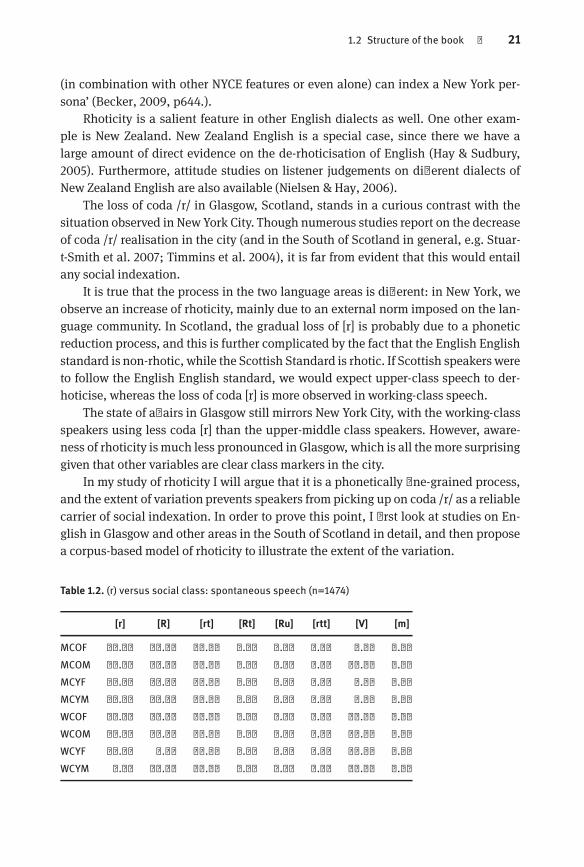
Table 1.2. (r) versus social class: spontaneous speech (n=1474)
[r] [R] [rt] [Rt] [Ru] [rtt] [V] [m]
MCOF 23.10 52.71 21.66 0.00 0.00 0.00 2.53 0.00MCOM 12.37 64.21 10.37 0.00 0.00 0.00 13.04 0.00MCYF 13.71 60.48 22.58 0.00 0.00 0.00 3.23 0.00MCYM 14.71 52.21 28.68 0.00 0.00 0.00 4.41 0.00WCOF 11.00 39.23 26.79 2.39 0.00 0.00 20.57 0.00WCOM 18.39 44.44 23.75 0.00 0.00 1.15 11.88 0.38WCYF 14.84 4.52 20.00 0.00 0.00 0.00 60.00 0.65WCYM 2.17 19.57 28.26 0.00 2.17 0.00 45.65 2.17

22 | 1 Preliminaries
Table 1.2, cited from Chapter 7, demonstrates the case in point. It shows the extentof variation in the realisation of coda /r/ (that is, in cases where it is not deleted)in Glasgow in a study of Timmins et al. (2004), using the variants they propose tocover (r) variation. What we observe is a wide extent of variation, with eight differentcategories, strongly dissimilar to the New York City case, where the realisation of /r/is less variable.
Rhoticity in Scotland, then, provides an example of a variable not being salientdue to the phonetic properties of its realisations, and also shows the potential risks ofthe probability-based method of assessing variable salience.
1.3 Concluding remarks
The aim of this chapter was to give a general introduction to the notion of sociolinguistic salience, interpreted as an attribute of a linguistic variable, which allows thevariable to carry social indexation. In an outline of the rest of this work, the chapternoted that there is a difference in the social salience of variables that has to be accounted for and put forward a possible way of doing so, namely, invoking the notionof cognitive salience, based on relative frequency differences in language data.
Itwent on to showhow this notion canbeput to test using a corpus-basedmethodology, and then discussed the case studies contained in this work which are attemptsat doing so. We also noted that social salience plays a relevant role in linguistic modelling, giving us a further argument to grant it a solid, theoretical status.
2 Defining SalienceThe first chapter outlined the research programme explored in this work, which is theoperationalisation of sociolinguistic salience and the investigation of its relevance tolinguistic theory. This chapter focusses on the history of the term both in sociolinguistics and in related fields and proposes a working definition for the rest of thebook. First, in section 2.1.1, I have a look at previous sociolinguistic studies of salience.Though the term is widely used, there is no concord with respect to its exact meaning.It is established that salience singles out certain dialectal variables to carry social indexation, however, it is uncertain whether this difference is simply typological or ifthere is an external grounding to it. In the first case, the term is not much more thana useful heuristic for sociolinguists, and certainly does not deserve an entire book ofits own. I will side with the authors who believe that there is an external grounding tosalience as a property. I also follow these authors by looking for this grounding in thecognitive domain.
Therefore, in section 2.1.2, I go on to survey the term’s use in visual cognition,not only because it is the cognitive field where salience is best established, but alsobecause visual and linguistic salience work similarly. They assign a property to a visual/linguistic unit that renders it perceptually more prominent in an arrayof competingunits, which is crucial in caseswhere selective attention is useful or necessary. Section 2.1.3 has a cursory look at selective attention in hearing. In section 2.2, I attemptto give a solid definition of salience in sociolinguistics. Sincemy operationalisation ofsalience heavily relies on theories of categorisation and human learning capacities,the respective theoretical frameworks –most notably the exemplar theory of categorisation – and the relevant psycholinguistic evidence is surveyed in section 2.2.3.
I will argue that sociolinguistic salience is based on the information-theoretic notion of surprisal: a unit is salient if it shows up with a high degree of unexpectedness,that is, a low probability of transition, in the speech signal. This definition is in tunewith the ways the concept is defined and used in the cognitive sciences. It also splitsthe concept into two. We can talk about the cognitive salience of a variable, which directly follows from its surprisal, and its social salience, whichmeans that it is amarkerof social variation, salient to the members of the language community.
2.1 Salience as a general term
Linguists often talk about salient properties or entities. The usual interpretation of theterm in phonology is quite literal: a salient feature is more visible or noticeable bothfor the linguist and the languageuser. In this sense, salient is notmore than a synonymfor conspicuous or standing out. One can find examples for such interpretations of thisterm in Vihman’s work on the acquisition of phonology. Vihman & Croft (2007) talk

24 | 2 Defining Salience
about salient segmental positions and rhythmic patterns, which are acquired earlierby the child learner. These patterns are structurally more regular, occur consistently,and are easily noticeable, so the learner canprocure them faster. Salience is also a tangible property of phonetic segments: a palatal glide is more salient between two lowvowels than between two high vowels, since the formant transitions cueing the glideare much more visible between low vowels, these having markedly different spectra.In comparison, such an intrusive glide between two similarly high vowels will have nostrong formant cues, and differs only in the lack of syllabicity. So, wemight say that itis less salient.
Salience has a similar sense in morphology. Chapman (1994, 1995) establishes adistinction between morphological categories based on perceptual salience. According to Chapman, perceptually salient patterns are more likely to serve as bases of generalisations – they are, in a way, more productive. Her example is analogical vowellengthening in Swiss German. The core of her argument is that vowel lengthening regularly occurs with suffixation patterns that are salient, i.e. semantically and formallytransparent, and that this preference cuts across the distinction between inflectionaland derivational suffixes. That is to say, vowel lengthening will tend to occur with aconsistent pattern, which pairs a single formwith a single function. This transparencyis more important than any other property of the suffix, such as whether it is inflectional or derivational.
In this interpretation, a morphological pattern is more salient if it is less markedfrom the point of view of complexity. The preference for less marked structures isalso the central tenet of NaturalMorphology (Dressler, 1999). Natural Morphology approaches morphological processes from an information-theoretical point of view: amorphological structure is optimal or maximally natural if it is iconic, uniform, andtransparent. Here, salience is interpreted within the frame of morphology: the moreregular the pattern, themore it adheres to the structure, themore salient itwill be. Thisis slightly at odds with the phonetic interpretation of salience, where the maximallyunlikely or out-of-place pattern gets more attention.
The common ground of the two approaches is that they donot regard salience as aspecial, inherent property. In phonetics, the term solely refers to the physical properties that a segment displays in a certain environment. Inmorphology, this comes downto regularity. That is, it is a characteristic which follows from the unit’s placement ina larger structure.
In the common linguistic usage, salience is either to be interpreted as a simple segmental property, as in phonetics, or a descriptive term to cover a set of phenomena, asin the morphology example. It can also be associated with a general attribute that follows from themodel architecture. The present example of this is Natural Morphology,where salience is associated with a more or less clearly defined notion ofmarkedness.As noted in Chapter 1, such an approachmight be problematic in its own way.
What unites all these interpretations, at least from our point of view, is thatsalience is seen as a blank term, either involving a straightforward stand-alone inter
2.1 Salience as a general term | 25
pretation, or gaining interpretation through its connection with the rest of the modelstructure.
The difference in sociolinguistics, as we will see, is that the term salience aspiresfor a status as a stand-alone theoretical concept. The problem is that often the theoretical status is taken for granted, without any attempt to give the term an explicitdefinition. The evasive nature of the term is illustrated by the fact that, though thereexist a number of definitions of salience in the surveyed literature, none of them covers all the phenomena that are regarded as salient by other authors.
2.1.1 Salience in sociolinguistics
The starting point in discussions of sociolinguistic salience is the two possible behaviours typically associatedwith adialectal variable. Certain variablesmightbecometargets of various processes, such as analogical levelling, dialectal borrowing, stigmatisation, style shifting, and so on. It is hard to establish, however, why some variablesare prone to be targeted by such processes whilst others stay exempt. The distinctionbetween the two types of variables is stated by Labov (1972b), who establishes twomain categories to cover it.
Indicators vary with social stratification, but have no social interpretation. If wehave a standard and a non-standard dialect, an indicator variable will be different inthe two. Yet, non-standard speakers will not try to use the standard indicator variable when speaking the standard dialect, and this will not be noticed by the standardspeakers. Indicators do not show style-shifting, and their use by speakers does notinvoke value judgements from the members of the language community. They are notsubjects of naïve linguistic awareness either.
An example is /aː/ in Norwich, mentioned in the previous chapter. Another couldbe the use of the velar approximant in words like what, where in Northern versusSouthern American English – while some Southern dialects have it, it does not seemto be associated with Southern speech in general (Dennis Preston, p.c.). One problemwith indicators is their sometimes nebulous status with respect to speaker behaviour.Ideally, an indicator does not show style shifting – it is not used less in a formal setting or when reading word lists. It does not trigger negative listener attitudes either:people will not consider its use non-standard, even if it is actually typical of a non-standard dialect. There are, however, features, which are avoided in more formal settings, but have no social stigma attached to them: listeners will not regard using themas less formal or proper, not even implicitly. Another, more serious problem is that itis sometimes hard to tell why a certain feature is an indicator rather than a marker.
Markers correlate with a sociolinguistic identity. If a marker attaches to a non-standard dialect, speakers will try to avoid it in more formal style settings and will regard its use as base or erroneous. I already cited Northern vs Southern English English/ɑ/ as an example. Another classic one is rhoticity in New York City, a marker heavily
26 | 2 Defining Salience
associated with social class and formal style settings (Labov, 1972b). Markers do notneed to be explicit subjects of linguistic awareness. One can regard a speech variety asimproper without being aware of the marker which provoked this attitude – yet, whenyou remove the marker, the attitude disappears along with it.
There is one case where the marker status of a variable is indisputable. This iswhen it becomes so strongly associated with a particular dialect or sociolect that itturns into a subject of naïve linguistic awareness. The only rough criterion for a linguistic stereotype is overt commentary. As Rosewarne (1984) shows, Southern EnglishEnglish speakers are able to point at word-medial glottalisation (in words like ‘butter’), and often attribute it to slackness or carelessness, ‘having a lazy tongue’.
Preston (1996) drafts a typology of folk linguistic awareness, with a focus on itscomplexity. Language users can be wholly able to remark on specific features, whilethey only become aware of others if these are identified for them. Some differencesare not available for a conscious discussion at all. The accuracy and detail of naïveawareness can also vary. (This has been illustrated by the African American Vernacular realisation of /aɪ/ in Chapter 1.)
Labov’s distinctions, to an extent, match Silverstein’s (2003) notion of indexicality. Indexicality is put to use in the analysis of the local dialect of Pittsburgh by Johnstone et al. (2006). Linguistic units of the first, second, and third order of indexicalityroughly correspond to indicators, markers, and stereotypes. These concepts are moreabstract, however, due toSilverstein’s emphasis onhow linguistic formsacquire socialmeaning.
This summary gives the impression that a marker is something that ‘switches on’a particular dialect image in a binary, deterministic fashion. To give an example, extensive word-medial glottalisation in ‘butter’-type words will cause the listener to categorise the speaker as ‘naff’: lower-middle class or working-class, uneducated, andsocially immobile. We could conveniently skip this level of abstraction and say thatword-medial glottalisation in English English is ‘naff’ in itself, since it always reliablytriggers the same kind of social profiling. The problem with this, of course, is that theinterpretation of a marker can change as a function of time and space: it can carry different indices dependent on the region, the social class of the listener, and whether itis the start- or the end-phase of an ongoing sound change (more on this in Chapter 9).
Furthermore, our notion that a variable carries social indexation is based on listener reactions to it. These reactions, however, can be mixed and complex (as shownby the work of Preston), turning the indicator/marker distinction into a gradient andmulti-dimensional continuum.
If we accept that interpretation is relative, we could still argue that recognition isnot. That is to say, in overall similar dialects, the same variants are prone to becomemarkers and the presence of a type of variationwill inevitably carry social indexationin any other similar dialect.
Campbell-Kibler (2011) shows how the interpretation of markers is – contrary tothe above assumption – also dynamic. She looks at gay speech stereotypes in US En
2.1 Salience as a general term | 27
glish and notices that some variants do invoke particular stereotype personas, butonly in conjunction with certain other variants. If this conjunction is not present, avariant might invoke a completely different persona or remain unnoticed.
This is corroborated by a study of Copenhagen Danish /s/, by Kristiansen et al.(2011). They investigate the way differences in /s/ realisation are perceived by Danishlisteners. They find that the way fronted variants are interpreted strongly dependson which area of the city the speaker is assumed to come from, which, in turn, isconnected to social class – a fronted [s] can be associated with certain types of richupper-middle class Danish speakers living in one part of the town, or immigrantsliving in another part. As one of their participants notes, ‘if this person comes from[rich part of the town], he must be gay, if he comes from [immigrant area], he isa foreigner.’
Newer studies constantly question – not to mention the interpretation – the mereexistence of linguistic variables earlier researchers have taken for granted. A good example to this is the research on the perception of assumed gay stereotypes in EnglishEnglish by Levon (2006).
The present discussion necessarily simplifies this issue and talks about the perception of individual markers. This is not a necessarily flawed approach – some sociolinguistic variables, like (ing) realisation, are reliable markers by themselves, anda model proposed for single types of variation can be always extended to cover morecomplex (and more life-like) types of speaker interaction.
What seems to be certain is that, oneway or another, sociolinguistic variables canbe grouped along the indicator/marker dimension, that is, with respect to whetherthey carry social indexation. The question remains how a variable is selected (or promoted) to be a marker, and what the exact differences are between the two variabletypes.
Trudgill (1986), taking Labov’s dichotomy as a starting point, lists a number ofproperties that linguistic markers have (as opposed to indicators). His context is thatof dialect contact situations. These properties include:1. having an overtly stigmatised variant,2. having a high-prestige variant (indicated in the orthography),3. undergoing change,4. comprising a large phonetic difference,5. being contrastive.
He adds salience as an additional factor, with an external psycholinguistic grounding, lying in perceptual distinctiveness and speaker attitudes. A marker might haveextra strong salience (sic.) when the language users regard it as a particularly strongfeature of the target dialect. In this view, then, salience is neither the source of thedistinction between indicators and markers, nor between different types of linguistic variables in general, but rather, it is an additional property with an external basis. Pointing to perceptual distinctiveness and speaker behaviour implies cognitive

28 | 2 Defining Salience
roots: salience, then, is a trait a variable acquires based on its perception by individual speakers.
Kerswill & Williams (2002) examine Trudgill’s features and point to two generalproblems: the first is that while these features might serve as guidelines in establishing the marker status of a dialectal variable, they are not particularly helpful in deciding whether the variable, as a marker, will be accepted or rejected by language users.Their second objection is that bringing forward stigmatisation as a source of markerstatus – which in turn leads to stigmatisation – is circular. Kerswill and Williams addthat the only property they find unproblematic is the notion of contrast. This propertyimplies, however, that the variation of a marker has to affect a phonological contrast.Nonetheless, language users can be extremely conscious of dialectal variables whichdo not potentially entail neutralisation, as in the case of /t/ glottalisation in the Southof England (Fabricius, 2000). This suggests that the correlation between contrastiveness and marker status is not that clear-cut – a conclusion we ought to bear in minddespite the fact that the concept of phonetic distance, to an extent, covers contrastiveness as well.
As noted above, salience, in Trudgill’s interpretation, comes on top of all this,contributing to the marker status of a sociolinguistic variable. If we accept that, wehave to look for the origins of salience in the basic phonetic/structural properties,while it also remains rather imprecise how salience promotes a variable. While wecould also take a view of salience as a sum of these properties (and/or others), i.e.those that differentiate a marker from an indicator, this approach is problematic inits own particular way. It bereaves salience of any theoretical status, and reduces itto an alternative for marker. What is more, the inherent circularity remains, as theproperties of a salient variable, in this view, are precisely the ones that follow from itssalience.
Kerswill and Williams, partly following Trudgill, give a provisional definition ofsalience as perceptual and cognitive prominence. This is a point to which I will later return. They go on to illustrate that the term is far from being unequivocally established.Kerswill (1985) argues that themain prerequisite is phonetic discreteness, particularlyif it comes from the lexicalisation of a phonetic difference, his example being /l/ vocalisation in the South of England.
Auer et al. (1998) also start with the assumption that lexicalisation has a prominent role in the salience of a dialectal feature. In their study of East German immigrants’ adaptation of the local standard in West Germany, however, they find nostrong correlation between the lexicalisation of a feature and its adoption by language users. Their starting criteria are similar to Trudgill’s, but are in fact taken fromSchirmunski’s 1930 pioneering work on dialect contact situations in German speaking dialect enclaves in Russia. Schirmunski established a main difference betweenprimary (or salient) and secondary variables in dialect contact, resembling Labov’smarker/indicatordistinction. Schirmunski assumed six criteria that a salient dialectalvariable will typically meet:
2.1 Salience as a general term | 29
1. Articulatory/perceptual distance: The physical distance between two differing dialectal variants.
2. Lexicalisation: Whether the change affecting the dialectal variable proceeds in agradual or a categorical manner (see above).
3. Categoriality: Whether the variable constitutes a categorical or continuous phonetic difference.
4. Awareness: The extent of naïve linguistic awareness of the variable.5. Writing: The non-standard variant’s occurrence in writing, informal or formal.6. Comprehension: Whether a variable is intelligible between two dialects.
Auer and his colleagues note that while the first three of these criteria are objective, the latter three are subjective, and depend largely on the speaker or the speakercommunity. Applied to their study of East German immigrants in the West, they findthat lexicalisation can override all these criteria, and that, most notably, the subjective criteria do not prove to have large predictive powers at all. This leads themto question the general usefulness of subjective salience, and, indeed, salience ingeneral.
Kerswill & Williams (2002) note that understanding salience requires the consideration of a wide array of possible properties (including lexicalisation). They dismissattempts to write it off as a positive correlate of high frequency (cf. Bardovi-Harlig1987). Defining salience in such a way is also unfortunate as it goes directly againstthemost general interpretation, discussed at the beginning of this chapter: a phoneticfeature which is salient in its environment will remain so irrespective of its frequencyin a given chunk of speech.
Another strong argument against blaming salience on high frequency is deliveredby the studyof Labov et al. (2006),who show that if listeners associate a dialectmarkerwith low prestige, this will in turn take an effect on their judgement of speech inputeven when the marker is relatively rare in the input. Their case is the variable (ing),the varying velar/coronal pronunciation of the progressive suffix <-ing> (-[əŋ]/-[ən])in US English. In their study, the coronal variant of (ing) has ten possible repetitions inan attitude test, and the results showed that listeners pick up on it after around threerepetitions, and their attitudes do not change remarkably after that, irrespective of thenumber of further repetitions. The presence of such a threshold seems to contradict asimple matching of salience and high frequency.
This is by no means an exhaustive list of the properties associated with salience.For instance, Kerswill (2002), in the context of dialect contact, adds regional restrictedness to phonetic distinctiveness as a requirement.
Going back to Kerswill & Williams (2002), their conclusion is that salience is auseful term in sociolinguistics, despite the apparent haze surrounding its definition.They establish three components that any operationalisation of salience has to incorporate:
30 | 2 Defining Salience
The presence of a linguistic phenomenon whose explanation we suspect may be due to thesalience of the linguistic feature or features involved. Typically, the phenomenon will be aparticular pattern observed in language change, language variation, the variable behaviour ofindividual speakers, or the acquisition of a linguistic feature. In cases of language change andvariation, the linguistic features are items being transferred from one language variety to another through diffusion; however, diffusion-type mechanisms may hold for the other types ofphenomena as well.Language-internal explanations, such as the presence of phonological contrast, great phoneticdistance, internally-defined naturalness, semantic transparency, or a particular syntactic orprosodic environment.Language-external cognitive, pragmatic, interactional, social psychological, and sociodemographic factors. Some have a natural link with the linguistic features being adopted (e.g. thatbetween a syntactic feature and its pragmatic function), while others have an arbitrary relationship (e.g. the favouring of one vowel quality over another).
(Kerswill & Williams, 2002, p.91)
They stress that the language-external factors are essential in giving a circularity-freeexplanation to salience. They make several references to a link to a possible cognitivebackground; this further reinforces their earlier, provisional definition of salience ascognitive or perceptual prominence.
To sum things up, sociolinguistic salience, according to the literature, can be interpreted in two ways. First, it can be a tag applied to variables that carry social indexation, and subsequently behave differently in code switching and language contactsituations. In this view, salience is nomore than another term for the indicator/markerdistinction.
The other possibility is to find an external basis for salience. In this case, theterm is derived fromproperties outside sociolinguistics proper, irrespective ofwhethersalience selects only markers, a subset thereof, or an entire cross-cut of variables,which is independent of the indicator/marker distinction. If we try to find an externalsource, it can either come from speaker dynamics, that is, the social setting in whichlanguage is used, or the basic cognitive capacities of the individual speaker.
Opting for thefirst possibility, speaker dynamics,means thatwegiveuponfindinga universal definition of salience. That is, any linguistic variable could theoreticallybe chosen by the community to mark social indexation, independent of the variable’sproperties. This is the view embraced by Labov (1972b): he argues that all variablesstart out as indicators, and later become markers, when the linguistic change gainsenoughmomentum to be noticed by the community and, as a result, they become vessels of social indexation. This view of the social life of variables can be inferred fromhis Martha’s Vineyard study. According to the study, the local residents at Martha’sVineyard picked up on a shift of the realisations of the diphthongs /aw/ and /ay/ toseparate themselves from the summer residents. The small difference between the local and the New England dialect became amplified to mark social identity. At the be

2.1 Salience as a general term | 31
ginning of this phase, the diphthongs are only indicators of this difference, later, asthey start to be used for the assertion of the local identity, they become markers.
Labov (1994) discards this simple explanation on the relationship of indicatorsand markers, pointing to the fact that some variables never seem to become markersat all. This brings us back to the original question: if salience has an external basis,and it is not only social dynamics, one ought to find a general, perceptual groundfor it, a frame, that prefers some features to others. Both Trudgill (1986) and Kerswill& Williams (2002) point to general cognitive capacities as a source of sociolinguisticsalience. The supposition is reasonable, as some variablesmight be pickedupbecausethey are more highlighted in the course of acquisition or auditory perception.
If we accept that sociolinguistic salience has cognitive grounds, we might wantto turn to cognitive science to look at the term’s history there. Such a comparison between sociolinguistic and cognitive salience is helpful in two ways: a look at cognitivesalience can render defining sociolinguistic salience easier, while comparing the twofields can tell us more about the general properties of salience in perception. The firstfield to be covered is visual cognition, with a brief look at auditory cognition as well.
2.1.2 Salience in visual cognition
Salience, as a concept, is best established in visual cognition. This section discussesthe interpretation and use of the term in this domain. The next section tries to operationalise this notion in sociolinguistic research relying on the cognitive background.Besides seeing, I also talk about listening in section 2.1.3, though I will contend thatvisual cognition is a much more useful parallel, despite the fact that our topic isphonology, an undoubtedly auditory field. (The gesture patterns of sign languagesalso belong to the phonological domain, but sign languages remain unaddressed inthis book.) The overview is not a complete one. The contributions of Gestalt psychology and, more importantly, figure-and-ground literature (cf. e.g. Rubin 2001) remainunaddressed.
Wolfe & Horowitz (2004) argue that sensory information is an ‘embarrassment ofriches’ that the brain could hardly process all at once. This is even more germane invisual attention deployment, since visual perception is responsible for most of thesensory information we obtain. The role of visual attention, then, is to filter out therelevant information and ease the processing burden. This is where salience becomesrelevant: a salient object bulges out of its surroundings, and, consequently, it can become a focus of attention much easier.
Salience in visual cognition is usually interpreted as the property of objects in ourvisual field. Its relevance as such comes from the fact that the brain is incapable ofprocessing the visual input in its entirety, and, therefore, is forced to select. Attention deployment, the preference of certain parts of the visual input to others, can be

32 | 2 Defining Salience
regarded as a spotlight, focussing on different parts of the input scene (Treisman &Gelade, 1980; Crick, 1984).
There is no complete agreement on the spotlight view of attention deployment (cf.Desimone & Duncan 1995). What seems certain is the existence of an informationalbottleneck: since visual input cannot be handled as a whole, most of the informationis filtered out initially, and this filtering is guided by attention. Attention gating, theselection and filtering of ‘interesting’ bits, has two broad aspects. First of all, it takesplace in two steps: there is a quick, automatic sweep controlled by target detection,concentrating on the highly salient items in the input. This is followed by a slower,effortful, controlled sweep. The latency of the latter, but not the former, depends onpractice aswell as task difficulty (Weichselgartner & Sperling, 1987). The two separateprocesses of attention gating are in a strict correspondence with the two main sets ofinfluences, the bottom-up and the top-down ones.
Bottom-up effects are largely automatic anddepend on the stimuli. Salience, computed across the whole visual field, plays a weighty role here. Top-down attention deployment is volitional, task-driven, and is affected by aspects such as reward or motivation (Itti et al., 2002). In comparison with bottom-up effects, top-down ones arerelatively complex. For instance, Itti & Baldi (2009) argue that surprisal has a hugepart in the latter, though probably not the former. Their interpretation of surprisal,however, is not simply a mechanical one. They assume an object to be most surprising if it causes the largest change in the observer’s prior beliefs about the world, whichis something far more intricate than the surprisal of a red object projecting in a blackfield. In this connotation, the salience of a given object is a sum of possible motivations, the given task, the observer’s mental state, and so on.
In comparison, bottom-up effects are relatively straightforward.Wolfe &Horowitz(2004) give a list of attributes thatmight render an object salient in a visual field. Theirlist shows that these are very basic visual properties, such as luminescence or shape.They strongly debate whether more complex objects, even if they are frequently occurring, such as the human face, would be able to have an effect on bottom-up attentiongating. Furthermore, this type of attention is overtly sensitive to the relative complexity of the visual field. The search for a salient object is easy if it differs from the rest inonly one feature.
It is not very difficult to find the black pawn between the white ones in Figure 2.1,since it only differs from the rest in colour. The same is true for Figure 2.2. Here the difference is in a different feature, the shape, not the colour. Figure 2.3 is another matter.Here we have a difference of two independent features, colour and shape, so it mighttake a while to find the black queen. These three figures not only illustrate the roleof feature complexity in visual search, but also that salience is a property calculatedagainst the rest of the visual scene: the black pawn is not salient per se, but only incompanyof the white ones. As Itti et al. (2002) note, feature contrast ismore importantthan local feature strength. Parkhurst et al. (2002), in their bottom-upmodel of stimulus salience, go on to argue that the observer will prefer regions which are deemedto be more informative in the sense of Shannon (1948). The Shannonian notion of

2.1 Salience as a general term | 33
P P P P P P P PP P P P P P P PP P P P P P p PP P P P P P P PP P P P P P P PP P P P P P P PP P P P P P P PP P P P P P P PFig. 2.1. Difference of a single feature
p p p p p p p pp p p p p p p pp p p p p p p pp p p b p p p pp p p p p p p pp p p p p p p pp p p p p p p pp p p p p p p pFig. 2.2. Difference of a single feature
surprisal entails that informativeness is determined by the degree of uncertainty: themore unpredictable a point is, in comparison with its environment, the more salientit will be. To go back to our simple example, in Figure 8.2, a black pawn’s colour willbe unpredictable based on its environment, whereas this will not be true for a whitepawn. Consequently, a black pawnwill bemore interesting for the observer, and it willbe the first target of attention. This is an overarching property of salience, not only invisual cognition, but also in linguistics. Salience is a relative concept: it is always interpreted in a context.
Models of attention gating assumea saliencemap (Itti et al., 2002; Koch&Ullman,1985), which is used to locate points of interest in the visual field. To put it very simply,a saliencemap is calculated in the following way: an individual saliencemap is calcu

34 | 2 Defining Salience
k K Q k k k k QK k k k k Q k Kk k k k K k K kk K q Q k k k Kk k k k Q k k Kk k K K k k Q kk K k K Q k k kQ k k Q k K K kFig. 2.3. Difference in two features
lated for each of the relevant classificatory features (in our examples, these would becolour and shape), and then these are matched in order to find the most salient pointof the visual field.
There is no complete agreement on the top-down and bottom-up share of theworkload. What seems to be certain is that some properties of objects are salient inthe sense that they will jut out irrespective of the observers prior expectations or thesearch task. Itti et al. (2002) emphasise the importance of these properties: they arguethat the research on salience in visual cognition can be extremely relevant to fields ofapplication such as advertising. This is an interesting point, since the use of saliencein advertisements would mean the manufacturing of visual objects that divert attention. This is slightly closer to our general topic than discussions that limit themselveson the location of salient objects in a visual field.
In advertising, one would want – for instance – to design and place a banner thatsticks out and grasps the passer-by’s attention. Similarly, a language user needs linguistic units that they can use to express their social identity. These units also have tobe salient, so that the other language users notice them easily and are able to pick upon the social indexation they carry.
To sum it up, salience in visual cognition is a property of individual objects ina visual field. This property, however, is calculated on the basis of comparison withother objects. It ultimately derives from informativeness, degree of unexpectedness,or surprisal: the less predictable an object is, in comparisonwith its environment, themore salient it will be. Salience plays a prime role in bottom-up attention deployment,which is automatic, swift, and independent of the search task.

2.1 Salience as a general term | 35
2.1.3 Selective attention in hearing
Selective attention is also an issue in hearing. Auditory prominence belongs to a different level than sociolinguistic salience, and the two seem orthogonal. One examplethat is nonetheless relevant to this study is the cocktail party effect (Pollack & Pickett,1957). The term covers two related phenomena in auditory attention deployment: theability to filter out a single speaker in the noise coming from the chorus of other speakers and the background, and the capacity to monitor more voices simultaneously anddivert one’s attention to one of them if a prominent piece of information comes upin it. This is usually illustrated by our ability to take notice of somebody mentioningour name in a conversation at a cocktail party, even if we were paying attention to adifferent speaker – hence the name of the effect.
Arons (1992) gives an excellent summary of the phenomenon, from the point ofview of speech processing. The task of filtering out background noise from the inputof e.g. one person talking to us is trivial for humans, yet it always proposed a seriousdifficulty for computer-based speech processing. (This point is linked to the problemof speaker normalisation in speechperception. Exemplar-based approaches to speechperception, the advance of which in linguistics happened in the mid to late 1990s, tryto tackle the issue directly. This is touched upon in section 2.2.3 below.)
One seminal paper on selective attention is Cherry (1953). Cherry performs experiments where the test subject has to listen to two separate spoken messages. His mainobservations are that subjects are able to separate twomixedmessages – given enoughrepetitions – if these are distinct enough in vocabulary and content. The subjects’ ability to separate the messages deteriorates if they contain a large amount of ‘highly-probable phrases’ or prefabs, n-gramswhich occur together often in corpora (Bybee &Cacoullos, 2009). (Labelling these units as prefabs is somewhat anachronistic, sinceCherry’smethodology is different from that of Bybee and Cacoullos, for instance. Still,the general notion behind ‘highly-probable phrases’ and prefabs is the same.)
One of Cherry’s main conclusions is that listeners rely heavily on ‘transition-probabilities’ in the subject matter, voice dynamics, and syntax, when separatingtwo mixed messages, that is, deploying selective attention. His approach to attentiondeployment is information-theoretic (Shannon, 1948). He argues that listeners seemto keep track on transitional probabilities between units at various levels of speechand divert attention using these as banners. It is implicit in his argumentation thatselective attention relies on the Shannonian notion of surprisal, which is consonantwith the reasoning we find in visual cognition. Needless to say, it also supports, tosome extent, the theory of salience advocated here. The analogues of sociolinguisticand visual salience, such as the role of surprisal in both, will be elaborated in the nextsection.

36 | 2 Defining Salience
2.2 Operationalising sociolinguistic salience
2.2.1 Preliminaries
At a first glance, the meanings attributed to salience in visual cognition and sociolinguistics are completely unrelated. In the former, it is relevant to the selection of anobject in a single visual field. This problem does not even come forward in the latter,as we usually regard auditory processing as sequential. Even though there are highlighted domains in the auditory input as well, such as the spectral peaks (formants)of the sound spectrum of human voice, sociolinguistics, even sociophonetics, usuallytakes the first part of speech processing as granted.
The secondmain distinction follows from this one: in visual cognition, salience istypically interpreted over a given image, whereas in sociolinguistics, we look for entities (linguistic variables) that prove salient in the long run, in the sense that speakerscontinuously rely on them in social indexation. It is also important to note that whilevisual salience seems to affect the bottom-up processes of attention gating, so it is avery low-level factor in attention deployment, linguistic salience comes in at a muchhigher level. It is interpreted as a property of entities that have already been identifiedas segments of a given dialect spoken in a certain setting (by a specific agent, etc.).This computationally demanding frame of reference is missing in the selection of ared object in front of a black background.
These differences all follow from the sociolinguistic standpoint, which assumesthat salience is interpreted as a property of a dialectal variable in language change ora dialect contact situation. If we look at salience as a general characteristic, it is easyto find one main similarity. In both cases, an entity juts out due to its dissimilarityto the rest of the structure. Dissimilarity is not an inherent property. It is assessed incomparison with the rest of the structure: a red object is salient against a black background, but not against a red one. Similarly, a palatal glide is salient between openvowels, but not between closed ones.
This parallel is the strongest if we compare studies of visual salience with studieswhere the term is used to express phonetic prominence, since here the structure isthe environment of the entity: the visual background or the speech stream. As I willlater argue, a more general definition of salience in sociolinguistics needs us to takemore than just the ambient language into consideration – the observer’s (that is, thelistener’s) preconceptions play a central role.
Gauging the properties of a unit in relation to the whole structure of which it isa member is a fundamental structuralist tenet (de Saussure 1916/1995,Lévi-Strauss1955). According to structuralist reasoning, individual properties are not inherent;rather they are only interpretable within a larger system of reference. I will also rely
2.2 Operationalising sociolinguistic salience | 37
on this in my operationalisation, and establish the following link between the use ofsalience in visual cognitionand sociolinguistics: in the former, it is a property anentityassumes in relation to the rest of the visual field, whereas in the latter, it is a propertya variant assumes in relation to the language structure.
2.2.2 Defining salience
Relying on the various descriptions of salience in language and cognition, I am goingto define salience in sociolinguistics as follows: A segment is cognitively salient if ithas a large surprisal value when compared to an array of language input. A variablethat has cognitively salient realisations can, in turn, be a marker of social indexation,becoming socially salient for the members of the language community.
Surprisal here is an information-theoretic measure – the less likely the segmentis to occur in a particular sequence, the more surprising it is for the language user.The reasonwhy we can talk about surprisal is that the language input, the speech signal, is highly structured. This follows from two properties of the phonological system,namely, a restricted set of available segments and phonotactic patterns determiningthe succession of segments. It also follows from the less predictable dynamics of connected speech sequences.
Cognitive salience is, then, a separate term fromsocial salience. Cognitive salienceis an attribute of variation that allows language users to pick up on it, whereas social salience means that variation is already used to carry social indexation. Sociallysalient variables, I argue, are always cognitively salient (one way or another), whichmeans that the term salience can be used without a risk of confusion. Cognitivelysalient variables, however, are not argued here to be always socially salient – this is avery strong statement that needs more evidence to state and is quite likely also untruefor all cases.
My main unit of measure will be transitional probability (TP). The transitionalprobability of segments Y and X, p(Y ∣X), is the probability that, given segment X,the following one will be Y (Figure 2.4). It is calculated by dividing the occurrences ofXY with the occurrences of X in a given corpus. Its use in linguisticswas first suggestedby the eminent American structuralist, Zeilig S. Harris (1955).While this formulation implies that a completely unfamiliar segment will have thelargest surprisal value (as, based on prior knowledge, it will not be anticipated at all),
p(Y ∣X) = likelihood of pair XYlikelihood of X
Fig. 2.4. Probability of Y following X
38 | 2 Defining Salience
I restrict my observations to cases where surprisal is a combinatorialmeasure, that is,where we talk about the surprisal of segments that are regularly used in a language.The context of surprisal is always a comparison of two dialects of the same language,usually a standard variety S and a non-standard variety S′. The typical scenario lookslike this: the distribution of a segment X is different (usually less restricted) in S′ thanin S. What follows is that a speaker of S encounters X in positions in S′ where it ismuch less likely to occur in their own dialect. Consequently, X will be salient to theS speaker, and can carry social indexation. Mind that this correlation is not implied tobe symmetrical: while I will argue that, at least in a certain set of cases, salience is theprerequisite of being a social marker, not all salient features necessarily carry socialindexation. This is where social dynamics come in: salient variables constitute a poolfrom which language users can pick to assert social identity – but they need not useall of them.
Theother important effect of theuseof language in the community is that, throughinteractions with S speakers, the S′ speaker can also pick up the variable X and useit to assert social or geographical identity (cf. Silverstein 1998). As the sociolinguisticliterature shows, the two dialects do not need to be in a standard-non-standard relation. What is important, though, is that we relate two dialects of the same language toeach other. Since this will mostly be self-evident in the case studies, this was broughtup at this point only for the sake of completeness.
While the choice of words here (and, indeed, throughout the book) might implythe language user’s conscious participation, it has to be stressed that very few socialvariables become stereotypes, subjects of naïve linguistic awareness. Any talk of ‘jutting out’ and ‘pickingup’ of variables should be put in the context that these processesusually remain entirely out of any awareness or conscious control.
In order to clarify this interpretation of salience, we have to look at two aspects ofsegmental distribution in the speech stream. First, we have to see how the structure ofthe speech stream allows domains to be salient. Second, we have to find evidence thatlanguage users can rely on such information, e.g. information on transitional probabilities. This salience claim relies on speakers making vast generalisations based onthe statistical regularities available in the speech stream, which requires the speakersto extort and process these patterns. The following section elaborates on these twoaspects.
It is important to stress that this definition is usage-based. It assumes that language users rely on information extracted from the speech input. Even though abstract patterns, such as language-specific phonotactic constraints, have an influenceon transitional probabilities (TP-s), they can be only acquired from language in use.This has various implications for my theory which will be addressed in the next section.
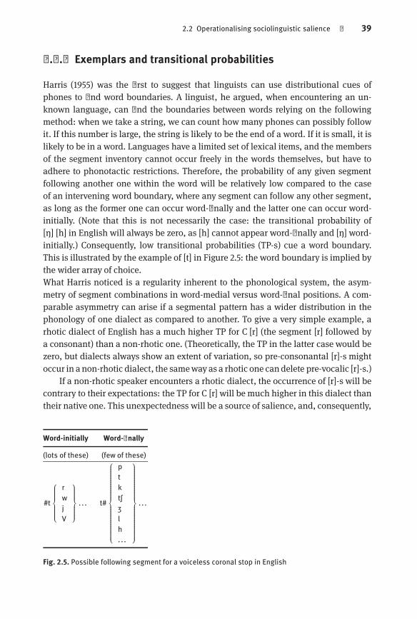
2.2 Operationalising sociolinguistic salience | 39
2.2.3 Exemplars and transitional probabilities
Harris (1955) was the first to suggest that linguists can use distributional cues ofphones to find word boundaries. A linguist, he argued, when encountering an unknown language, can find the boundaries between words relying on the followingmethod: when we take a string, we can count how many phones can possibly followit. If this number is large, the string is likely to be the end of a word. If it is small, it islikely to be in a word. Languages have a limited set of lexical items, and the membersof the segment inventory cannot occur freely in the words themselves, but have toadhere to phonotactic restrictions. Therefore, the probability of any given segmentfollowing another one within the word will be relatively low compared to the caseof an intervening word boundary, where any segment can follow any other segment,as long as the former one can occur word-finally and the latter one can occur word-initially. (Note that this is not necessarily the case: the transitional probability of[ŋ]∣[h] in English will always be zero, as [h] cannot appear word-finally and [ŋ] word-initially.) Consequently, low transitional probabilities (TP-s) cue a word boundary.This is illustrated by the example of [t] in Figure 2.5: the word boundary is implied bythe wider array of choice.What Harris noticed is a regularity inherent to the phonological system, the asymmetry of segment combinations in word-medial versus word-final positions. A comparable asymmetry can arise if a segmental pattern has a wider distribution in thephonology of one dialect as compared to another. To give a very simple example, arhotic dialect of English has a much higher TP for C∣[r] (the segment [r] followed bya consonant) than a non-rhotic one. (Theoretically, the TP in the latter case would bezero, but dialects always show an extent of variation, so pre-consonantal [r]-s mightoccur in a non-rhotic dialect, the sameway as a rhotic one candelete pre-vocalic [r]-s.)
If a non-rhotic speaker encounters a rhotic dialect, the occurrence of [r]-s will becontrary to their expectations: the TP for C∣[r] will be much higher in this dialect thantheir native one. This unexpectedness will be a source of salience, and, consequently,
Word-initially Word-finally
(lots of these) (few of these)
#t
⎧⎪⎪⎪⎪⎪⎪⎨⎪⎪⎪⎪⎪⎪⎩
rwjV
⎫⎪⎪⎪⎪⎪⎪⎬⎪⎪⎪⎪⎪⎪⎭
. . . t#
⎧⎪⎪⎪⎪⎪⎪⎪⎪⎪⎪⎪⎪⎪⎪⎪⎪⎪⎨⎪⎪⎪⎪⎪⎪⎪⎪⎪⎪⎪⎪⎪⎪⎪⎪⎪⎩
ptktʃʒlh.. .
⎫⎪⎪⎪⎪⎪⎪⎪⎪⎪⎪⎪⎪⎪⎪⎪⎪⎪⎬⎪⎪⎪⎪⎪⎪⎪⎪⎪⎪⎪⎪⎪⎪⎪⎪⎪⎭
. . .
Fig. 2.5. Possible following segment for a voiceless coronal stop in English
40 | 2 Defining Salience
rhoticity will be a possible candidate for social indexation. (As expected, rhoticity isa social marker on both sides of the Atlantic, as in New York City (Labov, 1972b) orBristol (Wells, 1982).) Before we get carried away with the possible applications, oneconcernmust be raised. Harris thought of TP-s as information available to the linguist,who, given a sizeable corpus, can compute it and use it to find the word boundaries.
There is abundant evidence, however, that language users are also able to rely onsuch information (Jusczyk et al., 1994, 1999; Saffran et al., 1996a,b; Cairns et al., 1997;Pierrehumbert, 2003; Hay, 2000). Psycholinguistic research concentrates especiallyon infants’ ability to segment speechbased ondistributional cues. Jusczyk et al. (1994)investigate 6 and 9month-old infants’ preference of high versus low frequency phonological patterns in the native language, which is, in this case, English. Theirmethod isto play lists of CVC shaped non-words to groups of infants. The hypothesis is that thesubjects will pay attention to familiar (that is, more frequent) patterns longer. Theyfind that the older age group shows a significant preference for patterns that occur inthe native language with a higher frequency. This remains true even if the input setsare matched for vowel quality. That is, even if the vowels are identical in the non-words with the different patterns, older infants still prefer the high frequency ones.This suggests that frequency is the only cue that the subjects rely on.
Saffran et al. (1996b) perform similar tests on adult learners. Their subjects have toacquire an artificial language consisting of noncewordswhichwere based on English,but are highly simplified. The input is a continuous stream of the nonce words readby a speech synthesiser. The only cues the subjects can use are the TP of nonce syllables, all of which have a CV form. The subjects are then tested using a list of words,some of whichwere built up from syllables which never occurred next to each other inthe input, i.e. their TP was zero, and some which were built up from syllables whichregularly occurred next to each other. The results are that performance is significantlyhigher than chance in the recognition of the ‘words’ of the input. These forms consistof syllables that occurred next to each other in the training input. This means that thesubjects could recall the TP-s of the input phase in the test phase.
Cairns et al. (1997) provide an overview of models of speech segmentation. Theynote that while top-down cues, such as the knowledge of the existent word forms ofthe language, have a large impact on segmentation, bottom-up cues, like TP-s, playan important role as well. They duly note that there are problems with approachesexclusively relying on TP-s in segmentation. For instance, even if we ignore top-downeffects, which makes sense if the subjects are acquiring the language, there are stillother strong factors in play, such as prosody: ninety per cent of English words haveinitial stress, which provides a reliable cue on word segmentation. Silverman (2006)argues against artificial language experiments (such as the two described above) onthe grounds that by excluding all noise (the effect of prosody and lexeme recognition,for instance) they create an unrealistic setting for language acquisition, which normally includes all possible cues, including the pragmatics and the setting. It is also

2.2 Operationalising sociolinguistic salience | 41
true that, according to certain studies, such as Yang (2004), frequency plays a verylittle role in language acquisition.
Bearing all this in mind, the argument holds that TP-s are available to the language user – even if the user does not depend exclusively on them. In order to put thisclaim in a broader context, and use it in operationalising salience, we need a theoryof reference which is able to accommodate information drawn from language use –like TPs – in speech perception. This is not a trivial problem, since the classic view ofspeech perception has no room for such information. The classic view of speech perception regards it as a de-coding process, which reconstructs the message containedin the input signal, after stripping it from everything except the bare essentials.
This happens in the following way: let us assume that a speaker directs an utterance towards the listener. This utterance is processed as speech (and not as howlingof the wind, for instance). Subsequently, it is normalised. This is necessary, since, forexample, the formant values of vowels, the main cues of vowel quality, can vary dependent on the speaker’s age and gender – and the corresponding difference in thesize of the vocal tract. The listener reconstructs the canonical vowel phones of theinput by, for instance, establishing normalised formant values by comparing the formants of the utterance to the general formant value ranges of the speaker (Gerstman,1968). This is called speaker normalisation. This way the listener recovers a detailedphonetic form from the highly variable input signal. This is then turned into an abstract phonemic representation by a phonological module (Chomsky & Halle, 1968).The phonemic representation is then interpreted bymatching it to the entries of wordsin the listener’s mental lexicon. The mental lexicon consists of similar abstract representations. In such a model, there is no toll taken of statistical patterns, since theincoming utterances are de-coded sequentially, one by one.
The view that speech perception involves speaker normalisation is challenged byJohnson (2005b). Johnson uses an exemplar-based model of speech perception. Insuch a model, all utterances are stored by the listener in rich phonetic detail. No abstract category prototypes or underlying forms are posited. The stored utterances, theexemplars, are categorised based on auditory properties, as well as external categorylabels, such as identity, age, or gender of speaker, context, and so on. Categorisationinvolves comparing the new exemplar with each of the remembered instances of thecategories, and the choice of category is based on the sum of similarity over each competing category. This leads to a self-organising behaviour in the mental lexicon, as exemplars will cluster up in distinct categories instead of spreading homogeneously inthe category space (Wedel, 2004).
Exemplar-based perception is not restricted to speech. Nosofsky (1988) showsthat an exemplar-based model fares better in predicting human subject behaviour incolour categorisation than alternative prototype-based models. An exemplar model’smain advantage is that they can model frequency effects better. Since categories areflexible and are able to shift under the influence of newmembers, the effects of different token frequencies readily follow from the model’s architecture.
42 | 2 Defining Salience
The usual argument against exemplar-based categorisation is that storing all theindividual instances takes up too much memory space, and is simply impossible.While exemplar-based theories involve a large amount of hierarchical structure andother measures to tackle this, Johnson (2005b; 2005a) also notes that human beingsseem to have a huge memory capacity, as suggested by experiments on identificationand recognition both for words and pictures (Goldinger, 1996; Standing et al., 1970).
Exemplar-based models give us a picture of speech perception that is radicallydifferent from the classic one. The input utterance is not de-coded, rather it is compared to already existing utterances to determine the category to which it belongs.An important consequence is that category selection is not only sensitive to the semantic content (what the speaker actually said), but also to minor details correlatingwith speaker age, gender, and identity. That is, there is a vast amount of informationavailable to the languageuser beyond the conveyed content. This is the reasonwhy exemplar theory enjoys widespread popularity in sociophonetics (Foulkes & Docherty,2006) – it is the only model of the mental lexicon capable of incorporating all the observed variation. One example of sensitivity to context and speaker identity is Glaswegian (Stuart-Smith, 2007a), which neatly illustrates how linguistic innovation in theworking class is closely connected to social dynamics and network structures.
As I wrote in Chapter 1, an utterance carries two indices, the actual meaning andsocial indexation. Exemplar theory allows us to refer to the latter, as it enables usto take sub-phonemic variation into account, which usually carries social indexationand which would not fit into an abstractionist model of the mental lexicon.
A standard objection to exemplar models is that they seem to leave too much leeway for variation, which can be problematic in category formation, and it poses a difficulty in sociolinguistics as well. If people are able to use detailed phonetic information, how come they are sensitive to certain linguistic variables, but not to others? Thisis where the present formalisation of salience comes into the picture again.
An exemplar-based model of the lexicon allows for the presupposition of transitional probabilities as active factors in speech perception, since a detailed, episodicword storage can contain frequency information (Pierrehumbert, 2001). It comes tomore than this, however, since an exemplar-basedmodel, in turn, needs our notion ofsalience to explain why people pick out certain variables, but not others, despite thefact that theoretically, all are available to carry social indexation.
In this view, salience follows from frequency: a unit with low relative frequency inthe structure becomes salient, and if this unit constitutes a part of a linguistic variable,the variable itself also becomes salient.
Linguistic variables which involve variants with low TP-s (in the context of comparing dialects) emerge as salient in an exemplar-based lexicon, since they constitute hotspots of attention in the range of information available to the language user.A variable with realisations that have a low TP, i.e. a high surprisal value, can be reliably used as a sociolinguistic marker since it is salient irrespective of the social indexation it carries. By relying on variables which already have variants with a lapsed

2.3 Concluding remarks | 43
distribution, i.e. behave erratically, the language users narrow down the set of possible carriers of social indexation, which makes both the deployment and recognitionof social markers easier. To put it simply, speakers will assert their social identity byusing features that are easily noticeable anyway. I will revisit this argument in detailin Chapter 8.
2.3 Concluding remarksThis chapter provided an operationalisation of sociolinguistic salience, couched in anexemplar-based model of perception, the dominant framework used in sociophonetics. Theargumentwas that linguistic variableswith ahighvalueof surprisal are salientfor the language user, and can be used for social indexation. This is in line with theresearch on the subject in sociolinguistics, where the difference between two types ofvariables, indicators, and markers, is widely acknowledged. Sociolinguists also tendto attribute this difference to a notion of perceptual salience, which has an external,cognitive grounding.
We looked at the general notion of salience, which covers the sum of properties which make an entity outstanding in a given context. The sociolinguistic sense,though rather vague, is somewhat similar: certain variables are more conspicuousthan others, which results in their marked use for social indexation, ranging fromunconscious patterns of context-dependent style shifting to being subjects of naïvelinguistic awareness. Since sociolinguists tend to look for a grounding of salience incognition, we also briefly surveyed the term as used in visual cognition. Here again,it is a property of elements of a visual array that are sufficiently different from theirbackground to divert attention.
Following up on all this, I established salience as low transitional probability (TP)in a given dialect, compared to a norm dialect. In this view, a variable is salient because its behaviour is different enough from the norm (or another dialect) to be surprising for the language user. Defining salience as dependent on TP-s was paired upwith psycholinguistic research on listeners’ sensitivity of such statistical informationand the overview of a framework, exemplar theory, which is able to accommodate thistype of knowledge.
In an exemplar-based framework, almost all linguistic variation is recorded. Anydifference between two dialects can be singled out to be a social marker. Salience narrows down the set of possible variables, rendering social marking more robust andreliable.
In the next chapter, I discuss my methodology of modelling variable saliencebased on spoken corpora. The following chapters will give examples of linguistic features which are used as social markers and which are also salient in the above sense.These case studies implement our hitherto heavily theoretical formulation of saliencein sociolinguistics.


3 MethodologyThis chapter outlines the methodology used in the case studies, first in terms of general principles, second, through an actual example to walk the reader through thenumbers.
Section 3.1 goes through the main assumptions of modelling salience in sociolinguistics. Section 3.2 gives a broad introduction to the use of corpora in the analysis ofsegmental distributions whichmight lead to the rise of sociolinguistic salience, whileSection 3.3 is a minute, technical description of the method itself, through a simplified example. Section 3.3 is not necessary to follow the argumentation in the rest ofthis work. It is a supplement for those readers who are interested in the engineering,not just the broad methodology and the results.
The case studies compare the salience of a variable to its speaker evaluation. Dataon the latter is indirect (except in one case) and the methods used to collect it arenot surveyed in detail. The focus is on cognitive salience and the distributions of thevariable’s realisations that underlie it.
3.1 Cognitive salience: main assumptions andconsiderations
The core idea of this work is that a variable is cognitively salient if its realisations aresurprising. That is, they have low transitional probabilities in the signal for a listener,who has dialect S, and who encounters them in dialect S′, the dialect of the speaker.Surprisal is measured through the comparison of the transitional probabilities (TP-s)of the segmental realisations of the variable in question. The speakers have to be partof one language community, which usually assumes mutual intelligibility (for mostspeakers at least) and a shared physical space, such as a country or a city. In mostcases, salience emerges in discussions of local versus supra-local dialects – this isillustrated by the discussion of Philadelphia English in Chapter 6 of Labov (2001),where Labov considers the social evaluation of local innovations in Philadelphia asopposed to their variants in standard East Coast General American.
Cognitive salience plays a role in the interactions of S speakers and S′ speakers,where the two dialects effectively only have to differ in the distributions of the realisations of a particular variable. This is in line with the canonical interpretation ofa language variant found both in the work of Wells (1982) and Labov (1972b) (for regional and social dialects, respectively): two language variants differ in at least onelinguistic variable – though the popular dialects investigated in these works are typi
46 | 3 Methodology
cally constituted by bundles of variants, like Irish English orUpper-middle class speechin NewYork City. Then, through a series of interactions, the cognitive salience of a variable is established in the language community. A cognitively salient variable can thenbecome socially salient and acquire a particular interpretation.
This interpretation of a language variant is overly simple. As the work of Campbell-Kibler (2011) shows, two (or more) variants can be interpreted differently when juxtaposed in a particular dialect as opposed to being present in the dialect alone. Whatis more, while Labov et al. (2006) report on listeners picking up on a language variantthat differs from the supra-local dialect in the United States in exactly one variable(the velar/coronal pronunciation of (ing)), Levon & Fox (2012), using the methodology of Labov et al. do not find such clear-cut listener reactions to one stereotypicallanguage variable in the United Kingdom, (th) fronting.
Another factor to take into consideration is that language users are not likely tobe equipped with a single dialect, but are, to varying extents, in command of morelanguage varieties and can identify even more – this is quite intuitive if we use theterm language variety rather broadly, including social registers and stylistic choicesas well, that is, all cases where structured linguistic variation can be observed.
Bearing that in mind, we ought to see that the complexity overlooked in such amodel does not undermine the interpretation of cognitive salience as stemming fromsurprisal. How social salience follows exactly from cognitive salience is a problem thatrelates to the general question of how variables gain social indexation, and this question is beyond the scope of the present work.
Preston (2001, 2011) focus on how and to what extent a linguistic variable canbecome subject to speaker awareness, providing a dynamic account of this problemfrom the recognition of the variable up to the point where it carries social indexationwhich is interpretable by at least a subset of the language community – that is, whenit becomes a social marker.
The notion of cognitive salience presented in this work is a static one. The ideais that a variable can be salient if there is a possible background that allows its realisations to jut out; a context in which its realisations have a surprising distribution,one that is characterised by notable differences in transitional probabilities. We assess surprisal through creating a language model that approximates distributions inspoken language to see whether these distributions are, in a given context, interestingin any way.
We will see that, while the ideal case is like that in Chapter 4.1, where detailedcorpora are available to study the distributions of the variable’s realisations, in mostcases the assessment of cognitive salience has to make use of more immediatemeans,which renders it a balancing act between robustness and abstraction.

3.2 Cognitive salience: further assumptions | 47
3.2 Cognitive salience: further assumptions
The source of a variable’s cognitive salience is a difference in distributions – interpreted as transitional probabilities (TP-s) – of the segmental realisations of a variablein two dialects. In most cases, the first dialect is geographically or socially restricted,and this is the dialect where the marked variant is characteristic. The second dialecthas a broader usage, and can be regarded as a supra-local or standard variety.
The use of a dialect corpus, such as the Fred corpus (Kortmann et al., 2005) cangive a very close approximation of the dialect in use, even if we consider the artificialities of speech collected by linguists. (Labov (1966/2006) examines this problem indetail.) It is more difficult to pin down the standard or supra-local part of the comparison: constraints on sounding mainstream are muchmore present in perception thanin production, especially in England, where the classic standard variety, Received Pronunciation, is spoken by a small minority of the population – and is certainly far frombeing unequivocally accepted as the standard to the same extent by everyone.
I take time todefendmychoice of corpora in the individual case studies. Theaim isalways to find a robust corpus for both dialects, which are roughly from the same timeperiod (to exclude the effect of large scale sound changes) andhave similar speakers inthem. I interpret the dialect-standard relation, the source of salience, in one speakergroup or societal unit. If this unit is the size of a city or even a country, one can berelatively flexible with the structure and temporal dimensions of the corpora used. Inany case, I rank size above anything else, because I think the amount of data is themost important factor in the significance of the results, and it can override the effectof other factors.
On the level of segmental phonology, the known processes which can interferewith the results can be accurately diagnosed. This means not taking your corpus datafor granted, but rather paying close attention to understanding how it is structured.
At this point, the task is to pick a corpus, measure transitional probabilities relevant for the variable under scrutiny, and compare itwith another corpus. Themain difficulty lies in the domain of study, phonology. Phonological variation is not marked inwritten transcriptions of speech (in corpora consisting of conversation or interviews)and is absent from written language, which is not true for morphological or syntacticvariation.
Large, phonetically transcribed corpora are rare, unsurprisingly, given the timeand effort. There are notable exceptions, like the Necte corpus (Allen et al., 2007), butthe usual case is that audio recordings and accompanying written transcriptions areavailable, as in the Fred corpus. If one does not want to give up the robustness offeredby available corpora, one has to use written transcriptions to approximate phonological patterns.
In sum, the best case scenario for a study of transitional probabilities is a huge,phonetically transcribed corpus. The second best case scenario is a written corpus in

48 | 3 Methodology
which the variant in question is marked, even though the corpus uses orthographictranscription. This is the way things stand with Definite Article Reduction (see Chapter 4.1) in the Fred corpus. It is consistently marked in the interview texts, and sincerecordings are available formost of the texts, one can sample the audiomaterial to seehow exact the transcribers were.
There is, however, no information on the other phonological characteristics of thegiven dialect in the text, and this is where one has to resort to approximation. Mymethod is to transcribe the material automatically, using a script which replaces thewords with their citation forms in phonetic transcription. This amounts to no morethan phonologising the English alphabet, as it disregards dialectal features and connected speech phenomena. But since information is available on the phonologicalcharacteristics of the dialect, the phonological patterns relevant to the type of variation in question can be accurately tracked.
In below, I use the example of the variable (ing) in a Lancashire interview of theFred corpus. This variable entails the realisation of the suffix -ing as [ən] (as opposedto standard [əŋ]), which is marked in the transcription. If I phonologise the transcription relying on citation forms, I will overlook all other Lancashire features, such as differences in vowel realisation. I can still operationalise how often I find the suffix [ən]before consonant- and vowel-initial words, since no known Lancashire phonologicalpattern would affect the word-initial distributions of these natural classes. (As a matter of fact, the only relatively common phonological variable that does so in Englishis /h/ dropping, the deletion of [h] in the onsets of stressed syllables – ([h] is typicallynot realised in unstressed syllables at all. <h>-initial words, however, are not frequentenough for /h/ dropping to interfere with any other process in terms of frequency.)
The outcome is a model of the Lancashire dialect. It is not capable of reflecting allthe properties of this variety of English, but it can give the TP-s for the variant we areinterested in.
The end results are reliable, even though they were reached through intermediatemeans, the use of a citation form-based automatic transcription.What the methodloses with the abstraction it gains with the size of the material we can work with, andsize is especially importantwhen oneworkswith probabilities – the larger the sample,the more calculated probabilities will approximate the ideal. (This is precisely analogouswith tossing a coin.Herewe know that the probability of heads is, all other thingsbeing equal, 0.5, and themore observationswehave, that is, themorewe toss the coin,themore the actual ratio of heads, based on these observations, will approximate 0.5.)
Things get considerably more difficult when the variant is not marked in the corpus. In this case, the corpus can serve as the basis for the general phonological distributions in a dialect – with the complication of automatic transcription. The extent
3.3 Step-by-step corpus editing | 49
of the use of a variant can be assessed using independent measures, such as studieson the variant in the dialect. Here, the corpus and the study complement each other:the corpus gives the general speech patterns that are typical to the dialect (such assentence length, word length, or vocabulary), while the study serves with details onthe variant’s behaviour: frequency, environments, realisation.
This approach requires even more caution, as it inserts another step of abstraction: not only is the corpus automatically transcribed, but the extent of variant usage,on which the TP-s are based, is established through an external source. Still, if onepays due attention to the properties of the corpus and the possible risks of the abstraction, it is a powerful tool in assessing segmental distributions and variable salience.
As I note above, this is just a general outline of themethodology of this work,withthe individual case studies addressing the details. The case studies give examples tothe trade-off between various levels of abstraction and robustness when relying oncorpora in investigating sociolinguistic salience – including cases where the methodyields a negative result. The next section does not elaborate this methodology further.Instead, it offers a detailed description of putting it into practice, of interest to readerswho would want to know more of the particulars.
3.3 Step-by-step corpus editingThis section gives a detailed walkthrough of the corpus-based methodology usedthroughout this work. It is a technical description, suggested only for those readerswho are dissatisfied with the depth of the methodology in any given chapter – in thiscase they can return here to have a complete view of the process.
As I write in the previous section, the main aim of the method is to get a sensible approximation of segmental transitional probabilities (TP-s) in real speech. Realspeech is approximated by the use of corpora, spoken corpora, when possible, andsegmental TP-s are gauged by transcribing the corpora automatically, replacingwordswith their citation forms. The example I will use in this section is one sociolinguisticinterview from the Fred corpus, coded LAN 001.
LAN 001 is an interview with a 76 year-old female from Barrow, Lancashire. Thewritten transcript is a txt, with a word count of 14,400. It has a header (enclosedin square brackets), which contains recording information and transcriber’s notes,such as that the subject tends to ‘drop final -g’. This is followed by main speaker andrecording data, and the interview itself. Lines 20–40 are repeated verbatim (exceptline breaks) below. (The first twenty lines are like ll 21–24, notes on the recording. Fordetails, the reader should consult the Fred documentation.)
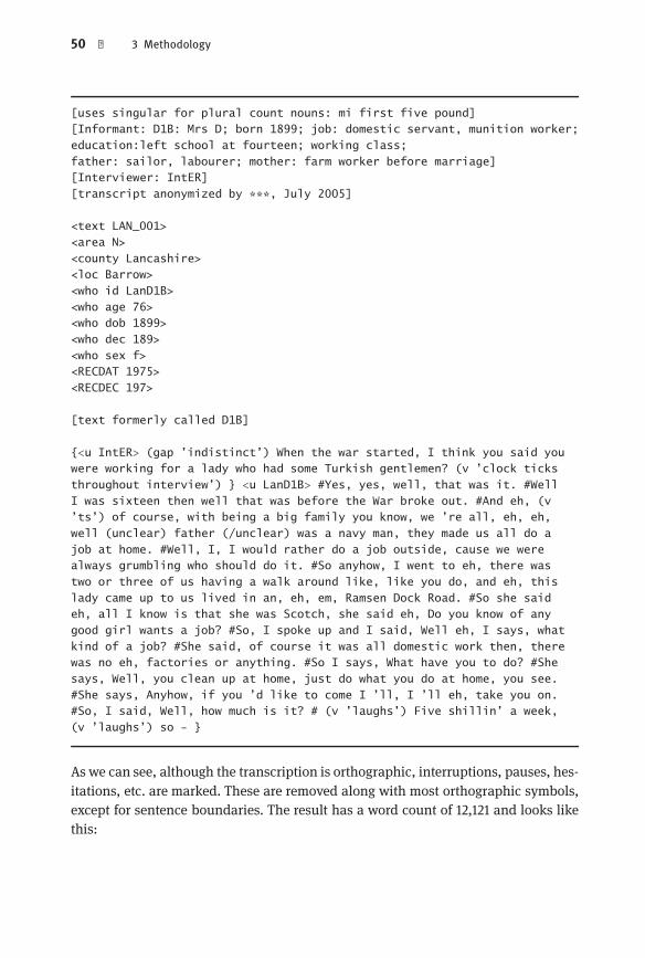
50 | 3 Methodology
[uses singular for plural count nouns: mi first five pound][Informant: D1B: Mrs D; born 1899; job: domestic servant, munition worker;
education:left school at fourteen; working class;
father: sailor, labourer; mother: farm worker before marriage][Interviewer: IntER]
[transcript anonymized by ***, July 2005]
<text LAN_001>
<area N>
<county Lancashire><loc Barrow>
<who id LanD1B>
<who age 76><who dob 1899>
<who dec 189>
<who sex f><RECDAT 1975>
<RECDEC 197>
[text formerly called D1B]
{<u IntER> (gap ’indistinct’) When the war started, I think you said youwere working for a lady who had some Turkish gentlemen? (v ’clock ticks
throughout interview’) } <u LanD1B> #Yes, yes, well, that was it. #Well
I was sixteen then well that was before the War broke out. #And eh, (v’ts’) of course, with being a big family you know, we ’re all, eh, eh,
well (unclear) father (/unclear) was a navy man, they made us all do a
job at home. #Well, I, I would rather do a job outside, cause we werealways grumbling who should do it. #So anyhow, I went to eh, there was
two or three of us having a walk around like, like you do, and eh, this
lady came up to us lived in an, eh, em, Ramsen Dock Road. #So she saideh, all I know is that she was Scotch, she said eh, Do you know of any
good girl wants a job? #So, I spoke up and I said, Well eh, I says, what
kind of a job? #She said, of course it was all domestic work then, therewas no eh, factories or anything. #So I says, What have you to do? #She
says, Well, you clean up at home, just do what you do at home, you see.
#She says, Anyhow, if you ’d like to come I ’ll, I ’ll eh, take you on.#So, I said, Well, how much is it? # (v ’laughs’) Five shillin’ a week,
(v ’laughs’) so - }
As we can see, although the transcription is orthographic, interruptions, pauses, hesitations, etc. are marked. These are removed along with most orthographic symbols,except for sentence boundaries. The result has a word count of 12,121 and looks likethis:
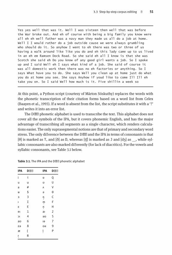
3.3 Step-by-step corpus editing | 51
Yes yes well that was it. Well I was sixteen then well that was beforethe War broke out. And eh of course with being a big family you know were
all eh eh well father was a navy man they made us all do a job at home.
Well I I would rather do a job outside cause we were always grumblingwho should do it. So anyhow I went to eh there was two or three of us
having a walk around like like you do and eh this lady came up to us lived
in an eh em Ramsen Dock Road. So she said eh all I know is that she wasScotch she said eh Do you know of any good girl wants a job. So I spoke
up and I said Well eh I says what kind of a job. She said of course it
was all domestic work then there was no eh factories or anything. So Isays What have you to do. She says Well you clean up at home just do what
you do at home you see. She says Anyhow if youd like to come Ill Ill eh
take you on. So I said Well how much is it. Five shillin a week so
At this point, a Python script (courtesy of Márton Sóskuthy) replaces the words withthe phonetic transcription of their citation forms based on a word list from Celex(Baayen et al., 1993). If a word is absent from the list, the script substitutes it with a ‘?’and writes it into an error list.
The Disc phonetic alphabet is used to transcribe the text. This alphabet does notcover all the symbols of the IPA, but it covers phonemic English, and has the majoradvantage of transcribing all segments as a single character, which renders calculations easier. The only suprasegmental notions are that of primary and secondarywordstress. The only difference between the Disc and the IPA in terms of consonants is that[θ] is marked as T, and [ð] as D, whereas [tʃ] is marked as J and [dʒ] as , while syllabic consonants are alsomarked differently (for lack of diacritics). For the vowels andsyllabic consonants, see Table 3.1 below.
Table 3.1. The IPA and the Disc phonetic alphabet
IPA Disc IPA Disc
i i ɒ Q
u u ʊ U
a # ʌ V
ʉ $ ə @
ɜ 3 ŋˈ
C
ɪ I mˈ
F
ɛ E nˈ
H
eɪ 1 aɪ 2
ɔɪ 4 əʊ 5
aʊ 6 ɪə 7
ɛə 8 ʊə 9
æ { lˈ
P
rˈ
R

52 | 3 Methodology
The end result is illustrated below:
’jEs ’jEs ’wEl ’D{t ’wQz ’It . ’wEl ’2 ’wQz "sIks’tin ’DEn ’wEl ’D{t ’wQz
bI’f$R ’Di ’w$R ’br5k ’6t .
This final output file has 11,522 words. This includes the 550 dots, which means thataround 1000 word tokens are missing after the conversion. Some of this difference issimply a residue of how word counts are calculated. Some missing words, however,are due to the conversion process: unknown words are transcribed as ‘?’, and theseare removed from the final output before TP-s are counted. As I note above, the scriptmakes a record of unknown words in a separate file. When working with larger corpora, I include words and transcriptions from the error list and transcribe the textagain. Infrequent proper names or idiosyncratic spellings are ignored.
In this example, the variant we are after is also spelled in an idiosyncratic way –where the informant realises a coronal variant of (ing), the original transcriber marksit with a dropped <g> in spelling, such as <shillin> for [ʃɪlɪn]. These are taken intoconsideration (cf. below).
In thepresent case, thefinal error list contains 197 tokens – this is the total numberof words missing from the output because they were not transcribed.
3.4 Calculating transitional probabilities
In the previous section, we arrived at the converted corpus text, the basis of comparisons. It is a useful basic tool, inasmuchas it is robust and it is basedonnatural speech.Its main weakness is that it consists of citation forms, so any dialectal phonologicalprocess that is present in the original has to be considered separately.
As I note at the beginning of this chapter, the easiest case is a corpus where thedialectal variant in question is alreadymarked, as in the case of DefiniteArticle Reduction. In thepresent case, one exampleof this couldbe thevariable (ing), the realisationof the suffix <-ing> ([əŋ]) as [ən]. The use of variants of (ing) is noted in the header ofLAN 001, and is marked throughout the text. The accuracy of the transcriber can beverified based on audio/visual inspection of the audio recording, or, if this would taketoo much time, parts of the recording.
To remain at the variable (ing), this is marked in the text by omitting the final ‘g’of the word (e.g. ‘shillin’ for ‘shilling’). Since these are not dictionary citation forms,they have to be included in the word list of the script separately. After the modificationof the word list, the script replaces these forms as having a coronal nasal ending. Thatis, ‘shillin’ will become [ʃɪlən] (or [’SIl@n] in the Disc alphabet). Similar systematicdeviations from standard spelling (such as <t’> for the reduced definite article) aretaken into consideration during transcription. After removing stress markers from the
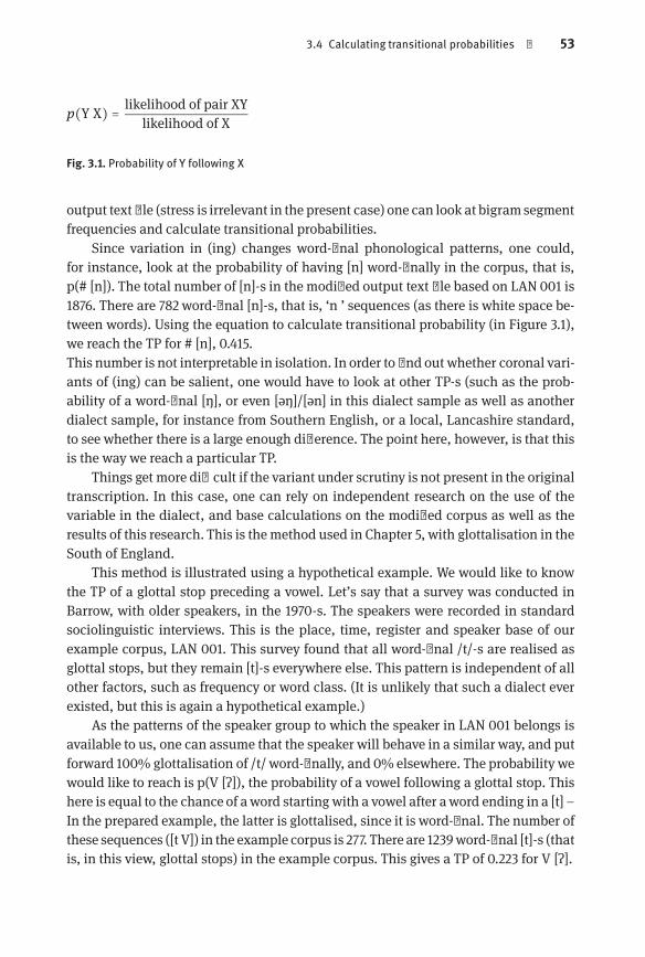
3.4 Calculating transitional probabilities | 53
p(Y∣X) = likelihood of pair XYlikelihood of X
Fig. 3.1. Probability of Y following X
output text file (stress is irrelevant in the present case) one can look at bigramsegmentfrequencies and calculate transitional probabilities.
Since variation in (ing) changes word-final phonological patterns, one could,for instance, look at the probability of having [n] word-finally in the corpus, that is,p(#∣[n]). The total number of [n]-s in the modified output text file based on LAN 001 is1876. There are 782 word-final [n]-s, that is, ‘n ’ sequences (as there is white space between words). Using the equation to calculate transitional probability (in Figure 3.1),we reach the TP for #∣[n], 0.415.This number is not interpretable in isolation. In order to find out whether coronal variants of (ing) can be salient, one would have to look at other TP-s (such as the probability of a word-final [ŋ], or even [əŋ]/[ən] in this dialect sample as well as anotherdialect sample, for instance from Southern English, or a local, Lancashire standard,to see whether there is a large enough difference. The point here, however, is that thisis the way we reach a particular TP.
Things get more difficult if the variant under scrutiny is not present in the originaltranscription. In this case, one can rely on independent research on the use of thevariable in the dialect, and base calculations on the modified corpus as well as theresults of this research. This is the method used in Chapter 5, with glottalisation in theSouth of England.
This method is illustrated using a hypothetical example. We would like to knowthe TP of a glottal stop preceding a vowel. Let’s say that a survey was conducted inBarrow, with older speakers, in the 1970-s. The speakers were recorded in standardsociolinguistic interviews. This is the place, time, register and speaker base of ourexample corpus, LAN 001. This survey found that all word-final /t/-s are realised asglottal stops, but they remain [t]-s everywhere else. This pattern is independent of allother factors, such as frequency or word class. (It is unlikely that such a dialect everexisted, but this is again a hypothetical example.)
As the patterns of the speaker group to which the speaker in LAN 001 belongs isavailable to us, one can assume that the speaker will behave in a similar way, and putforward 100% glottalisation of /t/ word-finally, and 0% elsewhere. The probability wewould like to reach is p(V∣[ʔ]), the probability of a vowel following a glottal stop. Thishere is equal to the chance of aword startingwith a vowel after aword ending in a [t] –In the prepared example, the latter is glottalised, since it is word-final. The number ofthese sequences ([t V]) in the example corpus is 277. There are 1239word-final [t]-s (thatis, in this view, glottal stops) in the example corpus. This gives a TP of 0.223 for V∣[ʔ].

54 | 3 Methodology
One important caveat of this method is that one has to pay attention to potentiallyintervening phonological patterns in the corpus dialect, because the results of theseprocesses are not marked in the transcribed corpus. As noted above, /h/ dropping canpotentially alter the amount of vowel-initial words, and therefore alter the TP above.One can assess whether a process is frequent enough (in terms of number of realisations) to have a strong effect.
This is the detailed outline of the basics of the method used in the case studies.In the case studies themselves, I elaborate on it and explain my choice of corpora,studies, and all the potential intervening factors.

4 Definite Article ReductionThe previous chapters introduced the notion of salience as a variable’s surprisal,which allows its use as a sociolinguistic marker. I also promised concrete examplessupporting this hypothesis. The first one of these, definite article reduction, is thesubject of this chapter. Though I defined salience as a general distinction in surprisalor novelty, in this chapter, I will argue that the variable in question is not only salientbecause of the different segmental distributions of its realisations, but also becausethese distributions enhance its role as a word boundary marker.
As wemight recall from Chapter 1, the original purpose of calculating transitionalprobabilities was finding word boundaries (Harris, 1955). Boundary markers and listener sensitivity to such elements in the speech string also feature prominently inTrubetzkoy (1939). Trubetzkoy, after looking through the taxonomy of boundarymarkers in various languages, comes to the conclusion that these are probably the mostconspicuous elements of the language input for any listener. Though my definition ofsociolinguistic salience is not necessarily connected to the boundary marking function of transitional probability differences, the variable examined in this chapter, definite article reduction, happens to be a casewhere the variable’s salience is reinforcedby the fact that the realisations of the variable are good word boundary markers.
Definite article reduction is an especially good case study of sociolinguisticsalience. In Chapter 3, I argue that, in order to assess the salience of a variable,one needs studies on the production and perception of its variants, as well as corporain which the patterning of its use can be directly observed. I also noted that the latter tends to be the weaker point of the exercise, because, even in a language as welldescribed as English, machine-readable corpus material of sociolinguistic variationis relatively scarce. The present case is an exception, because machine-readable material is available on the distributions of the realisations of the variable in naturalspeech.
This means that if the approximation of a salience model, as argued in Chapters 1and 3, is largely a trade-off between robustness (size of availablematerial thatwe basecalculations on) and abstractness (the proximity of the results to the ideal distributionof the variants’ use in spoken language), this study is the least abstract onepossible, asit is based on spoken language corpora that are available in sufficient size and detail.
The following chapters give examples where sociolinguistic salience has to be assessed in a more abstract manner. We will see that though the size of the availablematerial in these case studies is larger than in the present case, this comes at the costof an increase in the distance of the approximated distributions from ideal ones – oneswe would observe in natural speech.
Section 4.1 goes through the properties of the variable, as well as its literature,while section 4.2 explores its salience as a consequence of its probability distributions,with an emphasis on how these probabilities lead to the variants’ status as good word

56 | 4 Definite Article Reduction
boundarymarkers. Section 4.3 gives a summary and discusses the possible caveats ofthe analysis.
4.1 BackgroundThe term definite article reduction (DAR) refers to a dialectal variable in the North ofEngland, where the definite article has non-standard realisations. The variable appears everywhere with the exception of Northumberland, but is generally associatedwith the historic counties of Yorkshire and Lancashire. Contrary to what the term implies, DAR forms are not commonly regarded as reduced variants of the standard definite article.
4.1.1 Details of the process
The process itself is outlined by Wright (1905) who argues that the reduced definitearticle is a single voiceless stop before consonant-initial words and a voiceless dentalfricative before vowel-initial ones. Jones (1999) says that this view is oversimplified,pointing to the Survey of English Dialects (Upton et al., 1994), which lists 16 differentvariants. The most common ones are [t] (commonly with an extent of pre-glottalisation) and especially [ʔ], which suggests that the reduced article is a constriction, usually a glottal one. Some of the variants, like the dental fricative, only occur in certaindialect areas (from those that feature article reduction). Lodge (2010) gives the realisation of the definite article in parts of Lancashire and Yorkshire as the glottal stopboth before voiced and voiceless stops (cf. Table 4.1 for examples).
Various types of reduced articles can occur, along with the standard variant, inthe production of one speaker. This is illustrated by an excerpt from the Fred corpusbelow. The speaker is an 80 year-old male from Yorkshire, the reduced article is transcribed as <t’> or <th’>. This transcription here refers to a [ʔ] and a [θ] realisation.
And, the handyman that lived here, S(. . . ), they went into t’ s-, in that stable, with flames goingout ten foot high above t’ stable, all full length, because we ’d put, we had a loft full of hay, we’d just put two loads of hay up i’ t’ loft and flames coming out o’ t’ top, and all their manes, theracks was full of hay, and they were on fire, it burnt all the fringes, their fringes off, and th’ frontoff th’ horses.
Table 4.1. Reduced definite articles (examples from the Fred corpus)
the day [ʔdeɪ] the inn [ʔin]the pub [ʔpʊb] the apple [ʔæpl
ˈ]
the cooker [ʔkʊkə] the order [ʔodə]

4.1 Background | 57
Table 4.2. Grassington data on DAR use
broad polite totalt’ the t’ the t’ the
J 250 19 105 31 355 50B 72 5 648 41 720 46M 113 6 35 12 146 18total 435 30 788 84 1223 114
Not only does definite article reduction show considerable variation, it also alternateswith the standard variant of the article, the, with the latter occurring in certain contexts, such as in careful speech or in idioms.
The precise extent of the use of DAR is debated. On the one hand, it does not occurfrequently in corpora. Tagliamonte & Roeder (2009) find 13.7 per cent in their analysisof the York Corpus, and I also found a ratio of 13.8 per cent in the Yorkshire part of theFred corpus. On the other hand, Jones (2007) notes a much larger extent of DAR usein certain studies. His observation is corroborated by Glauser’s excellent descriptionof the dialect of Grassington, North Yorkshire (Glauser, 1984). He reports the directopposite of the Fred results (for instance), by putting the use of the standard form to8.5 per cent in the speech of three interviewees (cf. Table 4.2).
The findings of Jones and Glauser hint at a larger extent of DAR use in a more familiar setting. Glauser’s data have to be handled with care, though, as the reportednumbers are surprisingly low. In comparison, the average amount of definite articlesin the Fred interviews is much higher, around four thousand per interview (For instance, it is 5900 for the second Yorkshire interview and 3200 for the third one.)
Rupp & Page-Verhoeff (2005) point out that DAR forms seem to be favoured overstandard forms in case of familiar referents, connecting the use of DAR with information structure. In the York study of Tagliamonte&Roeder (2009), youngmale speakersuse DAR to an unexpectedly large extent, which hints at its role as an identity marker.This would also suggest that speakers use DAR to a larger extent with a familiar interviewer and suppress it with a standard speaker, which would explain the variationbetween the attested numbers in different studies.
Rupp (2007) and Jones (2002) agree that, in spite of the name of the process, thereduced variants do not come from the phonetic reduction of the standard definitearticle. The actual diachronic process giving birth to DAR is rather unclear, but wascertainly entangled with the reduction of Middle English determiners, and involvedanalogical levelling in favour of the [ʔ] forms.
In sum, DAR seems to be sensitive to the phonetic environment (the followingsegment and maybe even the preceding one), as well as the discourse structure. It isaffected by the social dynamics in the dialect areas, and has a large range of variants,some occurring only in restricted dialectal areas, others in overlapping larger ones.

58 | 4 Definite Article Reduction
Table 4.3. Conditions in the Jones 2007 study
they see t’sacks after. . . [ðe siː ʔ saks aftə]they seat sacks after. . . [ðe siːʔ saks aftə]they see sacks after. . . [ðe siː saks aftə]
These aspects interact: for instance, if there is a fricative variant, it can consistentlyoccur before vowel-initial words, confining the plosive variant to pre-consonantal environment, even though in another dialect, which lacks the fricative form, the plosiveoccurs everywhere. In general, the plosive is a glottal stop, but it can showupas a glottalised coronal stop, or only as creaky voice, which is possibly the auditory correlateof a non-complete constriction of the glottis.
The reduced articles vary with the standard ones, even in the production of onespeaker – largely, but perhaps not exclusively, depending on the formality of the register. Jones (2007) adds yet another aspect: glottal stops occur in standard English, aspre-consonantal and word-final voiceless stops, especially /t/, often debuccalise andbecome glottal stops. These glottal stops, however, differ from the segmental realisation of the reduced article. As he concludes from a three-speaker study, the latter areshorter and more variable than the glottal stops coming from consonantal lenition.
Jones links this difference to the presence or absence of a morphological boundary. His examples can be seen in Table 4.3. In the first example, there are twomorphological boundaries around the glottal stop (indicated by a <t> in the orthography):#they#see#t#sacks#. In the second example, the glottal stop belongs to the previous word: #they#seat#sacks#, so there is only one flanking the glottal stop. Thisadds yet another aspect to definite article reduction, that of word boundaries.
Jones’ other main finding is that DAR segments systematically differ from caseswhere there is no article at all. In the DAR case, there is always an extent of laryngeal activity, which strongly suggests that equating DAR realisations with nullarticles (which are also possible in the Northern dialects) would be misleading. Heclaims that there are systematic differences between the DAR glottal stop realisationand glottal stops that are allophonic realisations of [t], the latter being longer andmore prominent. The debuccalisation of /t/ is not the only possible source of glottalstops in standard (i.e. DAR-less) English English. Post-vocalic fortis stops are usually pre-glottalised (Wells, 1982), and vowel-initial words can have an initial glottalclosure (very much like in German), especially if they stand at the head of an intonation phrase (Dilley et al., 1996). How these different glottal stops behave from aperceptual-phonological point of view is a question to which I will later return.

4.2 Analysis | 59
4.1.2 DAR as a salient variable
There is a difference of opinion in the DAR literature, both on the different realisationsof the reduced article and on the extent to which these are used by the speakers. Whatcan be safely said is that in Yorkshire and Lancashire, the standard definite articledisplays non-standard allomorphy, occurring in 10-14 per cent of the cases, at least incertain registers, usually in the form of a glottal constriction, though fricative realisations are also possible.
DAR seems to fit most requirements of being a marker. It fits Trudgill’s extra-strong salience or Labov’s stereotype, though the two are not, strictly speaking, synonymous (cf. Chapter 1). As Jones (1999) notes, it has long been a tool of illustratingtypical Northerner speech and, based on their data, Tagliamonte & Roeder (2009)reach the conclusion that it plays an important role in establishing identity in the cityof York. (I have spoken to more than one people living in or coming from Yorkshirewho lamented on the local custom of ‘dropping your articles’.)
Considering all this, one can safely say that DAR is a dialectal marker, used to express social or regional differences. It is a feature that distinguishes DAR dialects fromthe standard spoken both in the North and the South. This leads us to the question ofsalience: if it is amarker, it must be salient. The critical question is where this saliencecomes from. In section 4.2, I will try to find a possible source of the salience of definitearticle reduction.
4.2 Analysis
This section investigates the connection between the salience of DAR and its transitional probabilities. I will argue that the main source of the variable’s salience is negative frequency, that is, low transitional probabilities in the signal. In the case of DAR,however, it is not self-evident that this is the only way salience can be linked to frequency. Consequently, I go through the possible other links between salience and frequency, to reach the conclusion that the most satisfactory account points to the roleof transitional probabilities, and, specifically, word boundary marking.
Section 4.2.1 discusses the methodology, section 4.2.2 enumerates the possiblelinks between frequency and salience, section 4.2.3 introduces an alternative approach, further explored by section 4.2.4, and section 4.3 provides an interim summary.
4.2.1 Methods
My main data source in this section is the Freiburg Corpus of English Dialects (Fred,Kortmann et al. 2005). It is a monolingual spoken-language dialect corpus which con

60 | 4 Definite Article Reduction
tains full-length sociolinguistic interviews with native speakers from the British Isles.It reflects the traditional varieties found there during the second half of the 20th century. It contains 2.5millionwords and 200 hours of recorded speech. The Northern English part of the corpus, used in this paper, contains approximately five hundred thousandwords. Themajority of the interviewswere recorded in the 1970s and 1980s. Sincethe corpus aims at regional rather than social variation, the majority of the speakersare NORMs – non-mobile old rural males. (65 per cent of the speakers are male and 74per cent are over 60.) The raw (pre-editing) word count is 11,821 for the Yorkshire part(eleven interviews) and 14,801 for the Lancashire part (twenty-three interviews).
The interviews of the corpuswere recorded by native speakers, and transcriptionswere performed by trained phoneticians, which means that Fred is a fairly reliablesource on dialectalmorpho-phonological phenomena. Nevertheless, any data onDARuse were double-checked using both the transcribers’ notes (available for each interview) and the recordings.
Other corpus-based results on DAR are also used as a reference. My main sourceon word frequency data is the Celex corpus (Baayen et al., 1993), which is essentiallya frequency list based on 17.9 million items. The reason why I do not quote word frequencies from the Fred corpus directly is that the difference in sizemakes Celexmorerobust and reliable as a data source. It does not have anything to say on connectedspeech sequences or definite article reduction, so generalisations on these come either from Fred or other studies.
4.2.2 Salience from token frequency
Going back to the original question, that is, why DAR is a salient variable, a simpleanswer would be that there is plenty of it. This assumption is, however, problematicin two ways. First, as we have seen in Chapter 1, the link between salience and hightoken frequency is debated. Second, the ratio of DAR in corpora is relatively low. Inthe Yorkshire part of the Fred corpus, reduced forms make up 13.8 per cent of all thedefinite articles. This ratio is 9.2 per cent in the Lancashire part. This is, however, nota trivial issue. I have already touched upon other surveys, such as Glauser (1984) onGrassington, reporting higher extents of DAR use.
On the one hand, one can stress that lower DAR use appears to be typical of contact situations (where dialect speakers are in interactionwith a non-local interviewer).This is the reason for the lower numbers in the corpus studies. Salience is assessed inprecisely such situations, which could justify using the lower ratios in a discussionof the variable’s salience. On the other hand, as I note above, the direct link betweentoken frequency and salience is empirically debated, which means the differences inDAR ratios could be, in this case, ignored altogether.
One could argue that around ten per cent of all definite articles, the numbers wesee in corpora, is still quite a lot. This is true on the lexical level, but definite article

4.2 Analysis | 61
reduction is amorpho-phonological pattern. As such, it shouldbe compared tophonological variables to see whether its frequency amounts to anything. One possible parallel is the debuccalisation of /t/ before obstruents (as in Gatwick, butler), a variablewhich entails the almost complete substitution of /t/ with a glottal stop in these positions, and which carries no social indexation, at least in the South of England (Fabricius, 2000). In a sample of the South-East part of the Fred corpus (wc.: 80,000), thereare 3290 [t] plus obstruent sequences, both word-medially and across word boundaries. In comparison, the number of definite articles in this sample is 3100. Ten percent of this number is 310, which is much smaller than the number of [t] plus obstruent sequences. Yet, the former is salient, while the latter is not. (The South-East partwas chosen because it contains no definite article reduction.) It is interesting to notethat the odds do not change in DAR’s favour even if we assume its widespread use –if all definite articles are realised as reduced articles, they still cannot outweigh thenon-salient /t/ glottalisation pattern.
Another hypothesis would be to assume that DAR is not salient by virtue of itslarge numbers, but rather because it prefers to co-occurwithmore frequent (precedingor following) collocates. If we assume an exemplar-theoretic lexical representation,all tokens are registered in the memory. Consequently, types with larger frequency ofoccurrence have stronger representations, which are easier to access. When, in turn,DAR goes more often with types that have strong representations in the lexicon, it willbe accessed more easily and therefore it will be more salient.
Siewerska&Hollmann (2011) lookat the frequencyof the collocates of the reducedarticle and find a tendency of DAR occurring with more frequent collocates on its left.DAR tends to prefer preceding prepositions, which are usually frequent in themselves.They admit, however, that this correlation is not clear-cut, as the standard articleoccurs often in prepositional phrases as well, and suggest that a better explanationwould be to link the preference of DAR to the prepositional schema.
I found no correlation between DAR and the frequency of the right hand collocate in the Yorkshire part of the Fred corpus. This right hand collocate is overwhelmingly the noun of the determiner phrase. The methodology was as follows: 134 DARcollocate types and 676 standard definite article collocate types were extracted fromthe Yorkshire part of the corpus (wc.: 80,000). Their frequency was gained from theCelex corpus, and a t-test was performed on the two sets, with the hypothesis that theDAR collocates are, on the whole, more frequent. The results refute this hypothesis, asthere is no significant difference between the frequency of the DAR collocates versusthe standard definite article collocates (t = −1.5509, df = 595, p-value = 0.9393). Thisresult can be accepted with two provisos: first, types, not tokens were used – sincethe token frequencies are given in Celex, no detail was lost, except for cases were onetype occurs both with DAR and the standard article, yet with overwhelmingly different proportions. The effect of this difference in variations, however, seems negligible.Second, frequencies come fromCelex, not the Fred corpus, and, as Siewerska &Hollmann (2011) also note, somewords are usedmuchmore often in the Northern dialects

62 | 4 Definite Article Reduction
than in general. Then again, frequency data from the former is still more reliable thanfrom the latter, due to the relatively small size of the Fred corpus.
4.2.3 Salience from transitional probability
After looking at other possible frequency effects, I return tomy original claim, namely,thatDAR’s salient status comes generally from its transitional probabilities and specifically from its status as a good word boundary marker. For the sake of simplicity, Iwill assume the segmental realisation of DAR to be a glottal stop. This move is warranted by the available data. For example, only 2.4 per cent of the reduced articles aretranscribed as fricatives in the Lancashire part of the Fred corpus. This ratio is belowone per cent in the Yorkshire part. However, assuming that all glottal DAR allomorphsare facsimile glottal stops is severely abstracting, and I will provide additional detailwherever possible.
The quirk in the analysis is that we do not look at the probabilities of DAR at wordboundaries. This would not lead very far for two reasons. On the one hand, if DAR isregarded as a separate segment, absent from the standard, itwill always be surprising,simply because the standard lacks it completely. On the other hand, it will be an excellent boundary marker, since it will always stand at a boundary, as articles are wont todo. (Though it is useful to stress the absence of article reduction in the standard, thestatement is something of a tautology, as the term standard in this paper is usuallyemployed to refer to a DAR-less dialect, even though it will be elaborated below.)
The assumption behind the use of TP-s in grounding the salience of DAR is that itis similar to segments already present in the standard, namely, glottal stops that resultfrom various phonetic-phonological processes, detailed below. DAR as phonologicalsegment, then, will not be totally surprising for the listener; the major difference liesin its distributions, not in its existence.
As stated above, salience comes forth in a dialect contact context, when a speakerof the standard encounters the speaker of a DAR dialect. This leads us to the questionof defining the standard in the context of definite article reduction. A trivial choicein England would be the Received Pronunciation (RP), or at least a regional varietythereof (Wells, 1982). While RP does not necessarily havemuch respect in the North ofEngland, its use canbe justified as it is a dialectwithout definite article reduction, andstandard, in the DAR case, refers precisely to such a dialect. That is to say, the qualityof the Strut vowel, for instance, is immaterial to the perception of DAR – though, ofcourse, not to the perception of the Northern dialect that contains it.
On the face of it, assuming RP as a starting point makes the job very easy: if theDARallomorph is regarded as a glottal stop, it will be a perfect boundarymarkerword-initially, as RP has no word-initial glottal stops. Therefore, if a standard speaker encounters a word-initial glottal stop, it will have perceptual prominence, as it certainlymarks a word boundary.

4.2 Analysis | 63
Table 4.4. Glottal stops word-initially
Segment DAR dialect Standard
[ɪ] 0.04 0.04[ə] 0.03 0.03[ʔ] 0.007 0.006
This claim has to be elaborated, however, as word-initial glottal stops do occur inEnglish, even if not phonemically. Vowel-initial words can have an initial glottal stop,much like in German. Dilley et al. (1996), in a study of five American English speakersin a radio speech corpus, puts the extent of initial glottal stops in vowel-initial wordsbetween 13 and 44 per cent. If our hypothetical standard speaker displays even thelower end of this variation (around 10 per cent), word-initial glottal stops ‘cease to beinteresting’.
The main point of comparison is the standard definite article. Its part adjacent tothe word is either [ə] before consonant-initial words or [ɪ] before vowel-initial ones.DAR can outperform the standard article as a boundary marker if it is less likely toappear in this position in the standard dialect as opposed to the DAR dialect. This isthe case ifweassumenoword-initial glottalisation for the standard, but this differencewanes if we put it around ten per cent, as seen in Table 4.4.
The numbers in this table come from the Fred corpus. They are probabilities forthe occurrence of the segments in the first column, word-initially. The DAR numbersreflect a dialectwith definite article reduction,while the Standardnumbers come fromthe South-East part of the corpus, which has no DAR (the use of this part is justifiedfurther below). As can be seen, in the DAR dialect, the probability that a word startswith [ɪ] or [ə] is 0.07, which is one order of magnitude greater than the probability ofa word starting with a glottal stop. This means that DAR is a good boundary markerword-initially, both in the dialect itself and in comparison with a DAR-less standard,where the vowel probabilities are roughly the same, but there are no (phonemic) glottal stops word-initially.
The situation drastically changes, however, if we assume word-initial glottalisation for even as little as ten per cent of the vowel-initial words in the standard (columnthree): now there is no strong difference between the DAR dialect and the standard,and, therefore, the status of DAR as a boundary marker diminishes.
Even so, by looking at both Dilley et al. (1996) and Jones’ study on DAR glottalstops and glottal stops resulting from [t]-glottalisation, we can assume that the threeglottal stop realisations are different. This could mean that word-initial DAR glottalstops remain prominent for a standard speaker irrespective of the extent of word-initial glottalisation in the speaker’s own output, simply due to its differing phoneticcharacteristics.
64 | 4 Definite Article Reduction
The only other process giving rise to glottal stops (or, at least, glottal constrictions)in English is the pre-glottalisation of fortis stops (Giegerich, 1992). Since this processis confined to the syllable coda (or, at most, to ambi-syllabic positions), it is irrelevantwhen it comes to the word-initial distributions. The situation is different word-finally:debuccalisation, the loss of placeof pre-glottalised fortis consonants, is fairly commonword-finally, so the occurrence of a glottal stop would not be unusual in this position.
This is, of course, a simplified account. Word-initial glottalisation only occurswith vowel-initial words, so DAR could remain a good boundary marker beforeconsonant-initial ones despite extensive glottalisation of vowel-initial words. In thesame way, word-final debuccalisation is, at least in higher registers, avoided before afollowing vowel-initial word (Fabricius, 2000), whichwould, again, render DARmoreprominent word-finally if a vowel-initial word follows.
4.2.4 Further arguments for phonotactic distinctiveness
So far I looked at phonological arguments for and against the prominence of DARword-initially and word-finally. As we could see, its status as a boundary markerlargely depends on the extent of other processes in the standard, namely, word-initialand word-final glottalisation, as these create similar sequences. Now I turn to thebehaviour of connected speech sequences involving DAR, to see, if these can provesalient in comparison with a standard. This section relies less on phonological arguments and more on statistical methods. DAR is still assumed to be a glottal stop,which, again, is phonetically interpreted as a glottal constriction of a varying extent.
Depending on the previous and the following word, the connected speech sequences involving DAR can come in four forms:C[ʔ]C (preceding consonant-final and following consonant-initial word)C[ʔ]V (preceding consonant-final and following vowel-initial word)V[ʔ]C (preceding vowel-final and following consonant-initial word)V[ʔ]V (preceding vowel-final and following vowel-initial word)
The two aspects of the markedness of these clusters come from (i) the likelihood thatthe above clusters might occur in the speech stream if the speaker’s dialect has DARand (ii) their general phonotactic markedness (low probability or outright non-existence). The first question can be answered by looking at the general probability ofwords ending or starting in vowels or consonants. I used the ratios extracted from theYorkshire part of the Fred corpus to get the probabilities of DAR occurring with thedifferent environments (cf. Table 4.5).
The way to find out the probability of DAR in a particular environment is to calculate the probability of that environment in the first place. In the case of _C∣C_, thelikelihood of finding this sequence is 0.65×0.66. Theprobability of a consonant-initialword following a consonant-final one is, then, 0.43, so given the null-hypothesis that

4.2 Analysis | 65
Table 4.5.Word boundary probabilities
Environment Fred-based (Yks)
_C 0.65_V 0.35V_ 0.34C_ 0.66
DAR has the same chance to occur anywhere, these sequences will be the most abundant. Needless to say, a cluster of three consonants with a glottal stop in the middleis extremely marked in phonotactic terms. It rarely occurs word-internally, and if theconsonants in question are stops, it does not occur at all, which also increases thesalience of such sequences existing by virtue of DAR.
It has to be immediately added, though, that the null-hypothesis of DAR equallyoccurring anywhere is refuted by the results of the multivariate analysis performed byTagliamonte & Roeder (2009) on parts of their York Corpus. They show that DAR hasa larger probability to occur after vowels (cf. Table 4.6). One aspect of the multivariate analysis is that DAR is more easily distinguishable when standing before a vowel-initial word. This might lead to a bias in the data collection, which, in turn, comes upin the results, which might lead to the preference of the pre-vocalic position being anartefact of the analysis. Still, even if we take these findings into account, the weight ofC[ʔ]C clusters does not becomemuch smaller in comparisonwith the others. AlthoughDAR – supposedly – occurs more after vowel-final words, these words are relativelyrare, and consonant-initial words are as preferred as vowel-initial ones (treating ap
Table 4.6. DAR and phonetic environment
Environment factor weights
After vowel 0.65After liquid 0.63After nasal 0.58After stop 0.25After fricative/affricate 0.10Before vowel 0.38Before approximant 0.50Before liquid 0.56Before nasal 0.58Before stop 0.51Before fricative/affricate 0.53

66 | 4 Definite Article Reduction
Table 4.7. DAR and connected speech sequences 1
Environment DAR Probability Markedness (example)
C[ʔ]C 0.43 very high feed ʔ catC[ʔ]V 0.22 high eat ʔ appleV[ʔ]C 0.22 low free ʔ dolphinV[ʔ]V 0.12 low throw ʔ orange
Table 4.8. DAR and connected speech sequences 2
Environment DAR Probability Ref: tc Ref: w-med c
C[ʔ]C 0.43 1234 300C[ʔ]V 0.22 4088 1305V[ʔ]C 0.22 4950 612V[ʔ]V 0.12 3860 927
proximants as vowels), if not more. Going back to the original question of connectedspeech sequences, the possible environments are listed in Table 4.7. The first columnlists the environments, the second one their probabilities to occur in a DAR dialect.The third lists phonological markedness levels. Column four gives examples. Markedness is interpreted here as the probability of these sequences in a standard dialect.
Table 4.8 supplements the previous one with reference data on the frequency ofsuch sequences in adialectwithout reduceddefinite articles, therebygiving substanceto claims onmarkedness. I used the South-East part of the Fred corpus (wc.: 80,000).The South-East was chosen because it is probably the closest to the linguistic normin England, and mainly because it is a dialect area without definite article reduction.What the numbers actually say, is, in fact, the number of the given sequences withan intervening [t], rather than a glottal stop. The reason for this is that /t/ is the mostliable to lenite into a glottal stop. It is especially prone to do so pre-consonantally, butalso to an extent intervocalically. (For the extent of /t/ glottalisation in the linguisticstandard, cf. Fabricius 2000.)
Here, column three gives the overall counts of the sequences in the corpus, whilecolumn four gives the word-medial counts. The former give a hint on the general surprisal levels: a C[t]C sequence is considerably rarer than a V[t]C one (we expect /t/glottalisation in both of these environments), while the former is more likely to occurthrough DAR than the latter. This, again, means, that definite article reduction will bethe most salient for a standard speaker in the environment where it is most frequent.
Column four connects DAR probabilities with word boundary marking. Since,again, C[t]C (practically, C[ʔ]C) is the least likely sequence within a word, it is themost likely one to mark a word boundary. Glauser (1984) discusses the phonetic reali
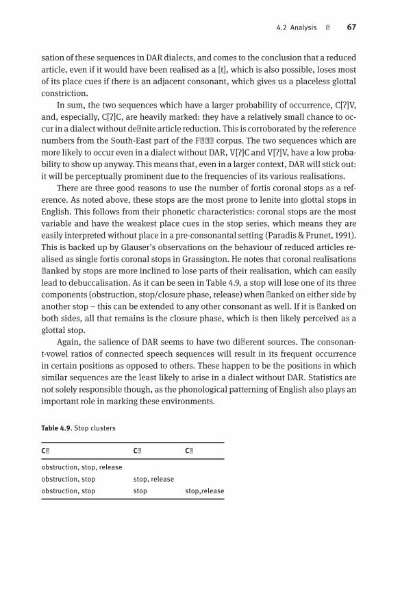
4.2 Analysis | 67
sation of these sequences in DAR dialects, and comes to the conclusion that a reducedarticle, even if it would have been realised as a [t], which is also possible, loses mostof its place cues if there is an adjacent consonant, which gives us a placeless glottalconstriction.
In sum, the two sequences which have a larger probability of occurrence, C[ʔ]V,and, especially, C[ʔ]C, are heavily marked: they have a relatively small chance to occur in a dialect without definite article reduction. This is corroborated by the referencenumbers from the South-East part of the Fred corpus. The two sequences which aremore likely to occur even in a dialect without DAR, V[ʔ]C and V[ʔ]V, have a low probability to show up anyway. Thismeans that, even in a larger context, DARwill stick out:it will be perceptually prominent due to the frequencies of its various realisations.
There are three good reasons to use the number of fortis coronal stops as a reference. As noted above, these stops are the most prone to lenite into glottal stops inEnglish. This follows from their phonetic characteristics: coronal stops are the mostvariable and have the weakest place cues in the stop series, which means they areeasily interpreted without place in a pre-consonantal setting (Paradis & Prunet, 1991).This is backed up by Glauser’s observations on the behaviour of reduced articles realised as single fortis coronal stops in Grassington. He notes that coronal realisationsflanked by stops are more inclined to lose parts of their realisation, which can easilylead to debuccalisation. As it can be seen in Table 4.9, a stop will lose one of its threecomponents (obstruction, stop/closure phase, release) when flanked on either side byanother stop – this can be extended to any other consonant as well. If it is flanked onboth sides, all that remains is the closure phase, which is then likely perceived as aglottal stop.
Again, the salience of DAR seems to have two different sources. The consonant-vowel ratios of connected speech sequences will result in its frequent occurrencein certain positions as opposed to others. These happen to be the positions in whichsimilar sequences are the least likely to arise in a dialect without DAR. Statistics arenot solely responsible though, as the phonological patterning of English also plays animportant role in marking these environments.
Table 4.9. Stop clusters
C1 C2 C3
obstruction, stop, releaseobstruction, stop stop, releaseobstruction, stop stop stop,release

68 | 4 Definite Article Reduction
4.3 Concluding remarks
In the previous sections I proposed that the reason behind the salience of definitearticle reduction is its unlikelihood in particular positions in the speech string. Thereduced allomorph is typically a glottal stop, and glottal stops have extremely lowprobability of occurrence word-initially. The same is true for clusters that might result from the insertion of a reduced article. As low transitional probability is exploitedby the listeners when processing the speech signal, reduced articles are perceptuallymore prominent and therefore more salient. What is more, they can enhance the discovery of word boundaries, which adds to this prominence.
The argumentationwas supported bymodels of Northern speech and the comparison of probabilities –which canbe seen as surprisal values for the listeners – betweendialects with and without DAR.
We ought to bear in mind a number of caveats. First, there is the problem of frequency. If we follow descriptions like Glauser (1984), and assumemuch larger extentsof DAR use, the argument for DAR’s position as a good word boundary marker stillstands. As a matter of fact, it is strengthened, since the more reduced articles are attested, the more robustly they can mark boundaries. The problem is, then, that thesalience of DAR could stem simply from its token frequency. There are two argumentsagainst this: first, at least in certain registers, DAR seems to have a low frequency –again, around ten per cent of all articles. Second, the seemingly intuitive connectionbetween high token frequency and salience is far from unequivocally established. Ifone insists on the role of the high frequency of the variants in the variable’s salience,it remains true that such a view is compatible with the analysis presented here.
Second, this account – and the whole book – takes a segmental phonological approach, which necessarily entails abstracting away from large amounts of phoneticdetail. Abstraction is a good thing, because it allows establishing wider generalisations on the data, without getting lost in the particulars. Still, whenever it felt needed,I explored the phonetic details of the environments involved, so as not to be ignorantof characteristics that would have otherwise been below the level of abstraction.
Third, low transitional probabilities are certainly not the only source of languageuser attention on the variable. Other possible reasons include the phonetic prominence of the reduced articles, as well as their possible interpretation as a null article.Null articles, though they feature in the Northern dialects, were consciously omittedfrom this discussion. It is possible, however, that a standard speaker, on encountering the reduced articles, would not regard them as articles at all, and, in turn, parsethe speech stream without definite articles. The resulting input string would lack definite articles, resulting in syntactic sequences that are ill-formed in the standard. Thiswould certainly be conspicuous and contribute to the salience of the variable in general.
4.3 Concluding remarks | 69
Fourth,while Imonopolised the concept of transitional probability for the segmental level, and talked exclusively about transitionsbetween segmental units, it certainlytakes hold supra-segmentally as well. The use of the reduced variant creates differentrhythmic patterns, which can lead to the increased salience of the variable. This remains true despite the fact that transitional probabilities, from Harris (1955) on, havebeen usually discussed in a segmental context. Then again, all of these factors arecompatible with the segmental probability-based analysis explored above.
The fifth and main caveat, in my view, is that the salience of the variable can bederived from the status of its realisations as good word boundary markers. One mightargue that the role of TP-s is, in this case, indirect, since the primary source of listenerattention is enhanced boundary marking. Indeed, this was my first suspicion whenapproaching article reduction.
Though boundary marking certainly adds to the variable’s salience, I believe itsmain source is still the difference in TP-s – in comparisonwith a standard dialect, lacking definite article reduction. Since the issue of boundaries and transitional probabilities is intermingled in the DAR case, a possible refutation of the argument connectingsalience to boundary marking would be to take an example where word boundariesclearly play a lesser role. In the following chapter, I turn to glottalisation in the Southof England, which is such a phenomenon. Though the question of salience, as we willsee, comes forward at a word boundary, this example is more about transitional probabilities, especially since themost stereotypical glottalisation environment, the word-medial pre-vocalic one, has nothing to do with word boundaries at all.


5 Glottalisation in the South of EnglandThe previous chapter introduced the method to establish a link between a variable’ssocial salience and the relative frequency distributions of its realisations using corpusdata. The case study in this chapter differs from thepreviousone inan importantway–it investigates a phenomenon in the case of which data on the distributions is notdirectly available. Rather, it has to be approximated through intermediate means. Inthis sense, approaching the social salience of glottalisation in the South of Englandfavours robustness to directness, involving a larger extent of abstraction.
The glottalisation of /t/ is awell-studied sociolinguistic pattern that occurs almosteverywhere in England and Scotland. In this chapter I look at its behaviour with anemphasis on its sociolinguistic salience. The scope of this discussion is the South ofEngland, and the glottalisation of /t/ word-finally. For the sake of simplicity, I ignoreutterance-final environments (which, in any case, occur with a small frequency) andthe glottalisation of other fortis stops.
Section 5.1 gives a brief overview of the development and distributions of the pattern in the South of England and argues for its sociolinguistic salience on the basisof external evidence. Section 5.2 describes the methods of the analysis, Section 5.2.4gives the analysis itself, while Section 5.3 provides a short summary.
I use the term /t/ glottalisation to refer to the glottal replacement, or loss of place,of the fortis coronal stop /t/ in the South of England. Glottalisation variably occursin all environments with the exception of a following word-medial stressed vowel orbefore a vowel word-initially. The process is phonetically motivated pre-consonantally. The phonetic ground is the glottal reinforcement of stops in English English(Giegerich, 1992) – in coda positions, the oral closure is reinforced by an accompanying glottal one. When we pair this up with the lack or release typical of pre-consonantal positions (Ladefoged &Maddieson, 1996), we end up with a stop that lost mostof its place cues, such as the formant transitions into and out of the closure phase.The result is the audible gesture of glottal replacement – a glottal stop. Coronal stops,being shorter and more variable in duration, are more prone to fall victim to glottalreplacement (Paradis & Prunet, 1991). Stops, however, can be subject to glottalisationbefore a vowel as well, a phenomenon both phonetically unmotivated and, as arguedbelow, salient. (John Harris (p.c.) points out that the place cues of a pre-glottalisedstop will be impaired even before a vowel, which can also lead to loss of place of articulation. What is certainly true is that this impairment is much smaller in extent thanin the case of a pre-consonantal stop.)
While /t/ glottalisation is a phonetically gradient phenomenon, stretching fromglottally reinforced coronal stops to complete loss of the coronal place of articulation(or debuccalisation), I will allow for the abstraction of regarding it as categorical, withword-final coronal stops realised either as coronal or as glottal. This is in line with theexisting studies (discussed below), which also operate with this level of abstraction,and still allows for a valid conclusion on the pattern’s salience.

72 | 5 Glottalisation in the South of England
5.1 Background
Glottal replacement is first reported in the South of England by Daniel Jones (Jones &Trofimov, 1923). It started out before a syllabic/vocalised sonorant (as in [bʌʔn
ˈ] ‘but
ton’, [bɔʔlˈ] ‘bottle’), and later spread to pre-consonantal, word-final, and pre-vocalic
environments (as in [fʊʔbɒːl] ‘football’, [tɑɡəʔ] ‘target’, [lɛʔə] ‘letter’, respectively).There are a number of older and more recent surveys on the pattern in the South.
An earlier example isHudson&Holloway (1977), a study of LondonEnglish conductedin 1977. The subjects wereworking class ormiddle class and between 14 and 15 years ofage. The results are that while Cockney, the traditional working class variant spokenin London, glottalised in all of the above environments (in 40 per cent of the casesin the intervocalic one), Popular London – spoken mainly by the middle classes inLondon – scarcely had signs of intervocalic debuccalisation, while the suburban accents had none at all. What is more, these accents shunned pre-syllabic liquid/nasalenvironments as well, only showing utterance-final and word-final pre-consonantaldebuccalisation in 20 per cent of the cases. (Near-RP and other high registers onlyglottalised word-finally, before a consonant, as in [ɡɛʔredɪ] ‘get ready’.)
The differences between the social groups remain in Tollfree’s study (1999),recorded between 1990-94, but there is a spectacular difference in numbers. Tollfree worked with two age groups (15-30 and 54-89) and two accent classes, roughlycorresponding to a middle class and a working class register. Unsurprisingly, theworking class idiolect has more debuccalisation, while the intervocalic environmentis still absent from the middle class variant. There is a great disparity between the1977 and the 1999 study, however, in the case of word-final pre-vocalic and pre-pauseenvironments. Tollfree’s numbers give five times more frequent debuccalisation inthese environments in the speech of the younger age group than in the data of theHudson & Holloway study.
The studies I am going to mainly rely on are Fabricius’ survey of upper-middleclass speech (2000) and Altendorf’s work on London English (2003). These are themost recent comprehensive studies on /t/ glottalisation in England.
5.1.1 Two recent studies
Altendorf’s scope is London and the Home Counties. In London, she looks at threedifferent school types, Comprehensive School, Grammar School, and Public School,which she roughly matches with working class, middle class, and upper-middle classlanguage use. Her results show that /t/ glottalisation happens across-the-board insome environments, while it shows variation, heavily related to speaker social classand register, in others. When it comes to the word-final environments, on the onehand, we can clearly see that working class speech glottalises almost all final coro

5.1 Background | 73
C #C ## #V L/N V_V
Environments
Ratio
0.0
0.2
0.4
0.6
0.8
1.0
Fig. 5.1. Lo-Co-Ca: Glottal replacement of /t/ in London (interview style) – from Altendorf (2003)
C #C ## #V L/N V_V
Environments
Ratio
0.0
0.2
0.4
0.6
0.8
1.0
Fig. 5.2. Lo-Co-Ca: Glottal replacement of /t/ in London (reading style) – from Altendorf (2003)

74 | 5 Glottalisation in the South of England
nal stops irrespective of whether it is recorded in a formal or an informal setting, whileupper-middle class speech avoids pre-vocalic glottalisation, especially in a formal setting. On the other hand, both classes glottalise almost every /t/ word-finally, beforea consonant. (Cf. Figures 5.1 and 5.2 – the columns indicate Comprehensive School,Grammar School, and Public School, respectively.) Another pattern Altendorf notes isthat glottalisation generally seems to be more extended in London than elsewhere inthe South, which is expected if we regard London as a source of linguistic innovationfor the area (and for England in general).Fabricius, in her dissertation, concentrates on upper-middle class speakers chieflyfrom London and the South (the Home Counties) to investigate the extent to which/t/ glottalisation is accepted in the speech of a younger generation of RP speakers.Her results corroborate the findings of Altendorf in two main aspects: first, /t/ glottalisation is more frequent in London than elsewhere in the South, second, it is commonpre-consonantally (independent of the register), while it is strongly avoided pre-vocalically, especially in a formal setting (cf. Figures 5.3, 5.4, and 5.5).
What both studies show is that /t/ glottalisation exhibits variation to the largestextent word-finally before a pause or a vowel, as well as word-medially. Variationseems to be sensitive on both the social background of the speaker (working classspeakers realising more glottal stops than middle or especially upper-middle classspeakers) and the register (all speakers realising more glottal stops in the interviewsetting than when reading a word list).
Stops Fricative Liq/Semiv Vowel Pause
Environments
Rat
io
0.0
0.2
0.4
0.6
0.8
Fig. 5.3. Glottal replacement of /t/ in interview style – from Fabricius (2000)

5.1 Background | 75
Stops Fricative Liq/Semiv Vowel Pause
Environments
Rat
io
0.0
0.1
0.2
0.3
0.4
0.5
0.6
Fig. 5.4. Glottal replacement of /t/ in reading style – from Fabricius (2000)
Stops Fricative Liq/Semiv Vowel Pause
Environments
Rat
io
0.0
0.2
0.4
0.6
0.8 London
Home CountiesRest
LondonHome CountiesRest
Fig. 5.5. Glottal replacement according to regions – from Fabricius (2000)
76 | 5 Glottalisation in the South of England
Altendorf’s results serve–amongwith the corpusdata–as abasis for calculationsin my analysis. As can be seen, her data are fairly congruous with Fabricius’ findingson upper-middle class speech. The extent of word-final glottalisation in working classspeech in her data are supported by previous studies and the observation of Paul Kerswill [p.c.] that /t/ glottalisation was not included as a variable in the analysis of theSpoken Corpus of Adolescent London English precisely because it was ubiquitous inall affected environments.
5.1.2 Salience and glottalisation
As seen in the previous chapter, from all the possible environments, word-final pre-vocalic /t/ glottalisation is subject to most variation. Three pieces of evidence suggest that it is salient for the language users. First, both the upper-middle class andthe middle class speakers glottalise less in the #V and ## environments in a formal setting; the feature shows style shifting. Though I restrict myself to the word-final environment (for now), all environments which display variation seem to showstyle shifting, which is strong evidence for the salience of glottalisation in general.Second, glottalisation, at least in certain positions, is subject to overt commentary. AsRosewarne (1984) notes in his seminal article on Estuary English, especially the word-medial glottalised realisations are regarded as base or erroneous by native speakers.The third piece of evidence comes from a discrimination study performed by Fabricius(2000). Fabricius tried to explore the attitudes of upper-middle class English speakerstowards /t/ glottalisation. Her input set consisted of 24 test sentences, recorded witha word-final glottal/coronal pronunciation. The nature of the following environment( #C or #V) was one of the variables. It was presented to 16 participants, 8 male,8 female.
The interviewees were asked to judge each pair according to which pronunciation they considered to be standard, good, correct. They were also told that theycould choose the first or second pronunciation, both, or reply that they didn’t know.An ANOVA analysis of the responses reveals a strong bias on the environment, i.e.whether the following word starts with a consonant or a vowel (p < 0.0001). The upper-middle class participants strongly favoured the coronal pronunciation before avowel, but significantly less so before a consonant.
Style shifting, stigmatisation, and negative listener attitudes all hint at #V glottalisation being salient for speakers of a conservative dialect (the one used by theupper-middle class speakers of the above studies). In contrast, we do not find styleshifting, or pronounced or unpronounced listener attitudes concerning #C glottalisation. This, again, indicates that glottalisation is not salient in this environment.
This gives us two variables to compare, word-final pre-vocalic andword-final pre-consonantal /t/ glottalisation. My hypothesis is that salience is based on differentprobability distributions in the conservative and in the innovative dialect. The former

5.2 Analysis | 77
will be modelled as spoken by the upper-middle class, the latter by the working class.The prediction, then, is that we observe different probability distributions across dialects in the case of the former, but not the latter environment: the salience of the #Vrealisation corresponds to a probability difference.
While the fact that /t/ glottalisation is overtly stigmatised in some cases is an argument for its status as a marker, salience is not necessarily connected to a threshold ofconsciousness. A variable, such as /t/ glottalisation, can, to all intents and purposes,behave like amarkerwithout any extent of naïve linguistic awareness. I amnoting thisin a continuing effort to keep the concepts of salience andmarker separate.
If we accept that #V glottalisation is different, we have to ask which aspectsmake it different from #C glottalisation. In both cases we are dealing with the sameprocess (loss of place), which only leaves the segmental environment as a potentialculprit. In the next section I propose an explanation for why the presence of a following vowel triggers a different perception of glottalisation.
5.2 AnalysisThere is no recent study which would be sufficiently large and encompassing for thepurposes of researching the salience of glottalisation. Consequently, my model isbased on two sources, transcriptions of spoken corpora collected in England on theone hand, and studies and descriptions of glottalisation in the South on the other.The corpora were used to get an approximation of upper-middle class and workingclass speech patterns. I relied on the studies to establish the extent of glottalisation,both because the corpora are not directly comparable, and because using the studiesleads to statistically more robust generalisations.
The aim was to establish transitional probabilities (TP-s) for the glottal stop inword-final position, depending on speech register, following environment, and socialclass. The hypothesis is that the salience of word-final pre-vocalic /t/ glottalisation(as opposed to the absence thereof in the word-final pre-consonantal environment)is directly related to the difference in TP-s between upper-middle class and workingclass use in the pre-V case, a difference not present in the pre-C case.
A crucial element of the argumentation is that word-final glottal stop variants isnot related directly and exclusively to word-final TP-s. This argumentation would be,in any case, circular: word-final pre-vocalic glottalisation is almost absent in upper-middle class speech, while fairly common in working-class speech, no wonder it issalient in the latter – from the perspective of the former. The present line of reasoninggoes one step beyond that: we start with the observation that glottalisation is presentin both dialects, and go on to note that, according to the model discussed below, theword-final distributions affect its general distributions in the two dialects. It is precisely this difference in general distributions that leads to the variable’s salience.
78 | 5 Glottalisation in the South of England
Word-final pre-vocalic glottalisation is, then, salient exactly because pre-vocalicglottalisation is salient in general. This claim predicts that all pre-vocalic incidents ofglottalisation should be noted by listeners – as we will see, this is indeed the case. Below, I look at the TP-s of glottal stops being followed by consonants and vowels in theword-final environment in particular, and in all environments in general. First, however, the transitional probabilities have to be established for the two assumeddialects,the upper-middle class and the working-class one.
5.2.1 Methods
In order to establish these probabilities, I used two corpora, the London-Lund Corpusof Spoken English for upper-middle class speech, and the Spoken Corpus of Adolescent London English for working class speech. Note that the two compared dialectsneed not be strictly tied to social class. One could regard the first dialect as the conservative, educated, non-local English accent – an approximation of the Received Pronunciation – and the second one as the local, innovative one, used by young peoplein London and in the South.
One issuewith using the two corpora is that one is simply older than the other: theLondon-Lund corpus, as discussed below, containsmaterial collected since the 1950s,while the Spoken Corpus of Adolescent London English was collected in a shorter period, in the mid-2000s. Given the alacrity andmomentum of glottalisation in England,one ought to be very considerate in comparing corpora (and studies) fromdifferent periods.
This, in my view, is still less of a problem: first, the older corpus is based on conservative registers and more formal settings, which tend to change less in the firstplace, second, in terms of the environments relevant for glottalisation in the presentstudy, the two corpora are fairly similar, despite the expected differences. This suggests that, when it comes to the word-final distribution of /t/, class differences areless pronounced in England. In any case, the fact that genuine samples of upper-middle class and lower class speech are available to compare is more important than thedifferences in the time of the data collection.
Since both corpora are fairly large – the London-Lund corpus has a size of roughly600,000 words, while the Spoken Corpus of Adolescent London English has a size ofroughly 1,000,000 – and /t/ glottalisation is not indicated in them, they were transcribed automatically, and both available information on the corpora themselves andadditional studies of /t/ glottalisation (most notably Altendorf 2003) were used to estimate its extent in the texts. (The corpora are described in detail below.)
While the size of the corpora would make transcription by hand very difficult, itgives very robust distributions of [t], so the TP-s of the [ʔ] realisation can be estimatedwith high accuracy. In comparison, the use of a smaller corpus, like parts of the corpora above, or the South-East part of Fred (Kortmann et al., 2005), would allow for
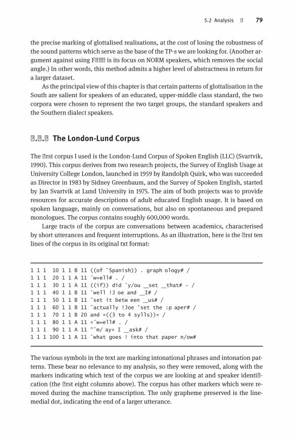
5.2 Analysis | 79
the precise marking of glottalised realisations, at the cost of losing the robustness ofthe sound patterns which serve as the base of the TP-s we are looking for. (Another argument against using Fred is its focus on NORM speakers, which removes the socialangle.) In other words, this method admits a higher level of abstractness in return fora larger dataset.
As the principal view of this chapter is that certain patterns of glottalisation in theSouth are salient for speakers of an educated, upper-middle class standard, the twocorpora were chosen to represent the two target groups, the standard speakers andthe Southern dialect speakers.
5.2.2 The London-Lund Corpus
The first corpus I used is the London-Lund Corpus of Spoken English (LLC) (Svartvik,1990). This corpus derives from two research projects, the Survey of English Usage atUniversity College London, launched in 1959 by Randolph Quirk, who was succeededas Director in 1983 by Sidney Greenbaum, and the Survey of Spoken English, startedby Jan Svartvik at Lund University in 1975. The aim of both projects was to provideresources for accurate descriptions of adult educated English usage. It is based onspoken language, mainly on conversations, but also on spontaneous and preparedmonologues. The corpus contains roughly 600,000 words.
Large tracts of the corpus are conversations between academics, characterisedby short utterances and frequent interruptions. As an illustration, here is the first tenlines of the corpus in its original txt format:
1 1 1 10 1 1 B 11 ((of ˆSpanish)) . graph/ology# /
1 1 1 20 1 1 A 11 ˆw=ell# . /
1 1 1 30 1 1 A 11 ((if)) did ˆy/ou set that# - /1 1 1 40 1 1 B 11 ˆwell !J/oe and I# /
1 1 1 50 1 1 B 11 ˆset it betw/een us# /
1 1 1 60 1 1 B 11 ˆactually !Joe ’set the :p/aper# /1 1 1 70 1 1 B 20 and *((3 to 4 sylls))* /
1 1 1 80 1 1 A 11 *ˆw=ell# . /
1 1 1 90 1 1 A 11 "ˆm//ay* I ask# /1 1 1 100 1 1 A 11 ˆwhat goes !/into that paper n/ow#
The various symbols in the text are marking intonational phrases and intonation patterns. These bear no relevance to my analysis, so they were removed, along with themarkers indicating which text of the corpus we are looking at and speaker identification (the first eight columns above). The corpus has other markers which were removed during the machine transcription. The only grapheme preserved is the line-medial dot, indicating the end of a larger utterance.

80 | 5 Glottalisation in the South of England
The texts were transcribed replacing words with their citation forms in Celex(Baayen et al., 1993) (for details, cf. Chapter 3). The extent of glottalisation was established using independent measures, namely, the available studies on glottalisation (more on this below). While other possible deviations from the standard are alsoabsent from the transcription, the effect of these is assumed to be minimal. This is especially true for the LLC, as it displays standard upper class speech. The resulting textlooks like this (for the ten-line excerpt above):
’Qv ’sp{nIS . ’wEl ’If ’dId ’ju ’sEt ’D{t ’wEl ’2 ’sEt ’It bI’twin ’Vs
’{kJ9lI ’Di ’p1p@R ’{nd ’tu ’wEl ’m1 ’2 ’#sk ’wQt ’g5z ’Intu ’D{t ’p1p@R
’n6
As we can see, the transcription is not perfect, for instance, it misses the proper name‘Joe’. It also removes line breaks, but since we are not interested in the utterance-final environment, and since this environment is not that frequent compared to otherones featuring [t], this is less of a problem. Citation forms have stressmarked on them.Clearly, not all words are equally stressed in fluent speech. However, word stress limits the extent of /t/ glottalisation (such as that /t/ is never glottalised before stressedvowels), so it is very useful as additional information. (A separate chapter discussesall the basic details of this corpus based method.)
The raw text of the corpus has 733,000 ‘words’ (including various annotationmarkers), of which 407,000 were successfully transcribed in the above fashion. Thistranscribed corpus is the basis for the model of upper-middle class speech. The distributions of [t]-s are given in Table 5.1.
Table 5.1. Transcription t-counts in the LLC
Environment Count
Pre-consonantal 13,500Word-final pre-consontantal 25,000Word-final pre-vocalic 11,875Utterance-final 1400Before syllabic sonorant 1400Intervocalic, before unstressed vowel 5700Intervocalic, before stressed vowel 800Other 37,925Total 97,600

5.2 Analysis | 81
Table 5.2. Coronal and glottal stop counts based on the LLC
Environment Count[t] [ʔ]
Pre-consonantal 0 13,500Word-final pre-consontantal 2250 23,750Word-final pre-vocalic 11,250 625Utterance-final 1400 0Before syllabic sonorant 1400 0Intervocalic, before unstressed vowel 5700 0Intervocalic, before stressed vowel 800 0Other 37,925 0Total 59,725 37,875
Table 5.2 shows the distributions of coronal and glottal stops in these environments,based on the formal (reading) data of Altendorf for London public school students.Note that, as opposed to the previous Table, these are estimated counts. The numbersare extrapolated from the Altendorf study, the ratios of whichwere applied to this corpus. What this Table shows, then, is an approximation on the extent of glottalisationin a conservative dialect of Southern English. The two sources of this approximationare a corpus of upper class language use and a study on upper class glottalisation –which study is corroborated by others of the similar kind, such as Fabricius (2000).These are the estimated that will allow establishing the transitional probabilities ofthe glottal stop in various positions – to reach its suspected salience as a variant inthese positions.
Bearing in mind the results here, we can turn to the second corpus, which is usedto model innovative, working class speech patterns.
5.2.3 The Spoken Corpus of Adolescent London English
The second corpus is the Spoken Corpus of Adolescent London English (SCALL) collected by Paul Kerswill, Jenny Cheshire, and their colleagues (Cheshire et al., 2008).The corpus contains interviews with adolescents (age 17-19) sampled from two London boroughs, between 2004 and 2007. The aim was to get a coherent picture of thelinguistic innovation present in adolescent speech in London, hence the focus onyoungworking class speakers. The corpus contains roughly 1,015,000words, of which1,005,000were successfully transcribed. Transcription followeda course similar to thecase of the LLC. One notable difference is that the SCALL focusses on working classspeech. It which might substantially differ from the citation forms used in the tran

82 | 5 Glottalisation in the South of England
scription process. These citation forms, taken from Celex, reflect RP. However, theeffects of these differences are assumed to be minimal.
To take one example, vowel qualities will be different in popular London speech,but that is outside this discussion. To take another example, some differences in theconsonant system might affect the loci of interest – word-final pre-vocalic and pre-consonantal positions. In particular, H-dropping could change the ratio of consonant-initial words, thereby affecting the distributions, but this is a small scale problem: inthe London English corpus, 305 tokens have an initial [h] – out of 1,005,000.
The SCALL has a different format from that of the LCC, consisting of standardsociolinguistic interviews with one or more participants, transcribed orthographically. Interjections, pauses, and hesitations are marked. Here is an example from thebeginning of the rawmaterial:
S(...): OK that should be it yeah erm I came over the week before last
I think it was [A(...): yeah] and you’d just gone out of the room forfor something [A(...): can’t remember] yeah no I don’t know where you
were so but erm
A(...): how long was I gone for?
S(...): I don’t know cos I only popped in there [A(...): ah] to findpeople and when I couldn’t find them I just came out again so [A(...):
oh] I was in there for about ten minutes or so <sniff> but er <throat
clearing> yeah erm the two that I spoke to before erm they..they werein the middle of assessment everybody 1 seems to be
After the removal of all the annotations and the machine transcription, the resultingtext looks like this (S(. . . )’s first utterance):
"5’k1 ’D{t ’SUd ’bi ’It ’j8 ’3m ’2 ’k1m ’5v@R ’Di ’wik bI’f$R ’l#st ’2
’TINk ’It ’wQz ’j8 ’n5 ’2 ’d5nt ’n5 ’w8R ’ju ’w3R ’s5 ’bVt ’3m
A few errors are obvious here as well. For example, the part between A(. . . )’s two interjections got lost along the way. Still, as noted above, the vast majority of the corpuswas transcribed successfully. The distributions ofword-final [t]-s are given in Table 5.3.
Table 5.4 shows the estimation based on the corpus and Altendorf’s reading datafor Comprehensive School. Note that in this case, we observe a much larger extent ofglottalisation than in the Table based on the LLC. This Table shows an approximationof glottalisation in the innovative, working class dialect of Southern English.
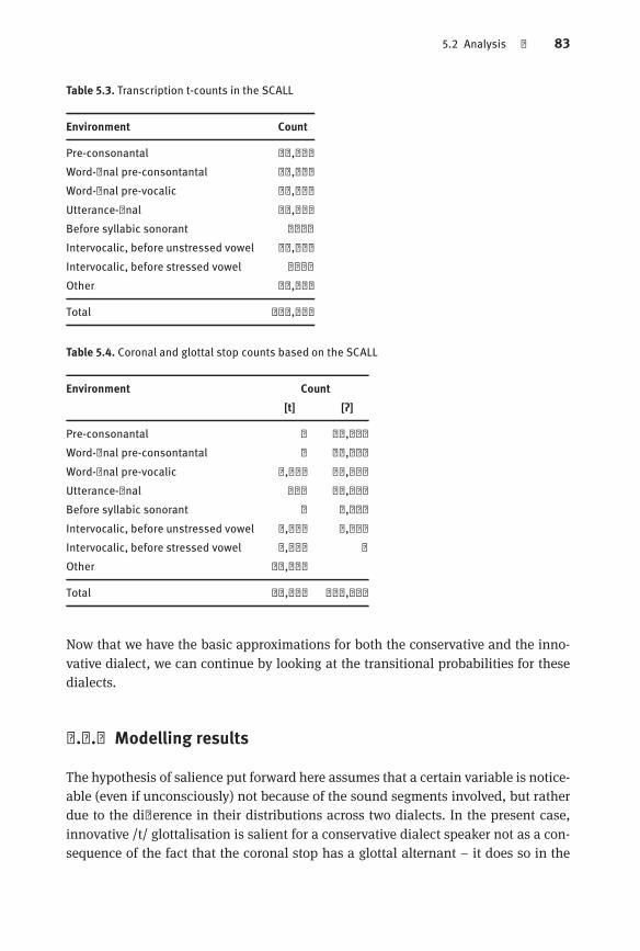
5.2 Analysis | 83
Table 5.3. Transcription t-counts in the SCALL
Environment Count
Pre-consonantal 29,900Word-final pre-consontantal 86,600Word-final pre-vocalic 36,000Utterance-final 15,500Before syllabic sonorant 2400Intervocalic, before unstressed vowel 12,700Intervocalic, before stressed vowel 1200Other 56,400
Total 239,300
Table 5.4. Coronal and glottal stop counts based on the SCALL
Environment Count[t] [ʔ]
Pre-consonantal 0 29,900Word-final pre-consontantal 0 86,600Word-final pre-vocalic 4,513 31,487Utterance-final 700 14,800Before syllabic sonorant 0 2,400Intervocalic, before unstressed vowel 9,271 3,429Intervocalic, before stressed vowel 1,200 0Other 56,400
Total 61,100 178,200
Now that we have the basic approximations for both the conservative and the innovative dialect, we can continue by looking at the transitional probabilities for thesedialects.
5.2.4 Modelling results
The hypothesis of salience put forward here assumes that a certain variable is noticeable (even if unconsciously) not because of the sound segments involved, but ratherdue to the difference in their distributions across two dialects. In the present case,innovative /t/ glottalisation is salient for a conservative dialect speaker not as a consequence of the fact that the coronal stop has a glottal alternant – it does so in the

84 | 5 Glottalisation in the South of England
Table 5.5.Word-final [ʔ] TP-s (formal)
Environment Conservative Innovative
p(#C∣ʔ) 0.627 0.486p(#V∣ʔ) 0.017 0.202
conservative dialect as well. It is the contrast in the glottal alternant’s distributionsthat makes a difference.
In this section I expand on the dialect models of /t/ glottalisation in various waysin order to compare estimated transitional probabilities in various environments.
The transitional probabilities of glottal stops and following consonant and vowel-initial words in the conservative and innovative dialects are given in Table 5.5. Thesenumbers are based on the models discussed in the previous section. As we can see,glottal stops aremore expected in both environments in the innovative dialect. This isnot really surprising given the fact that this dialect has a larger general extent of glottalisation. What is more noteworthy, however, is the extent of the difference in TP-sbetween the conservative and the innovative dialects. Pre-consonantally, the conservative TP is slightly higher. Pre-vocalically, the innovative TP is higher, and here, thedifference is much wider, one order of magnitude.What Table 5.5 shows, then, is a difference of TP-s in the twoword-final environments.Pre-consonantally, the [ʔ] TP-s are slightly different. Pre-vocalically, however, the difference is one order of magnitude between the two dialects, and the TP of [ʔ] in theinnovative dialect is much larger.
This is where TP-s and salience meet: since the pre-V distributions of the glottalstop are so different in the two dialects, this difference becomes a salient marker ofinnovative versus conservativedialect usage,which is reflectedbyavoidance in formalsettings, social indexation, and even overt commentary. Pre-consonantally, this splitis much smaller, therefore we do not expect salient behaviour from this realisation ofthe variable (cf. Section 5.1.2).
The higher TP of a consonant following a glottal stop in the conservative dialectmight seem counter-intuitive first. It is, however, entirely logical. TP-s are based onthe ratio of glottal stops in this position versus glottal stops in other positions, not onthe total number of glottal stops. Glottal stop realisations pre-consonantally have ahigher probability in the conservative dialect than in the innovative one, since, whilethe general extent of glottalisation is smaller in the former, the extent of pre-consonantal glottalisation is roughly the same. Therefore, a glottal stop is more likely pre-consonantally in the conservative dialect, irrespective of the ratio of the total numberof glottal stop realisations between the two dialects. (To put the findings in context,the overall probability of an orthographic <t> to be realised as a glottal stop is 0.388in the conservative dialect and 0.744 in the innovative one.)

5.2 Analysis | 85
The salience of /t/ glottalisation can be evaluated in a larger context. So far, welooked at the word-final pre-vocalic environment. The investigation can be extendedto all pre-vocalic environments, including word-medial ones. This is a useful step, assuch a larger context involves a stereotypical, highly stigmatised environment of /t/glottalisation, the glottalisation of /t/ word-medially, preceding an unstressed vowel.Examples of this environment are [’siʔɪ], [’lɛʔə], [’bʌʔə] (‘city, letter, butter’).
In order to calculate TP-s for this environment, one has to take into account theestimated glottal realisations word-medially, before stressed and unstressed vowels.For the former environment, there are no estimated glottal realisations based on thestudies. This is not surprising, since glottalisation is widely reported as absent in thisposition, so much so that surveys usually do not include it as an environment for thevariable.
As seen in Section 5.1, /t/ glottalisation is absent in this position in the conservative dialect, based on upper class speech in a formal setting. It is, however, present inthe innovative one, based on working class speech in a formal setting. Going throughthe same procedures as in the case of the word-final environments, we get the following TP-s for vowels following glottal stops in general, without respect to word boundaries:p(V∣ʔ) in the conservative dialect: 0.017p(V∣ʔ) in the innovative dialect: 0.254
Again, we find a large difference between the TP-s of the sequence in the two dialects,and it is much more likely to occur in the innovative dialect. This result, again, establishes a connection between the probability distributions of the realisation of thevariable and its salience: word-medial pre-vocalic glottalisation is much less frequentin the conservative dialect, hence the conservative dialect speaker attitudes towardsits innovative dialect use.
The case of word-final versus all pre-vocalic environments is relevant in twoways.First, it shows that the proposed method of TP calculation works for other environments as well, and is not an arbitrary way of singling out positions which would support the hypothesis. Second, it gives an empirical ground to the salience of word-medial pre-vocalic /t/ glottalisation, another salient realisation of the variable.
Formal interview settings served as the basis of calculations throughout this chapter. If we regard Altendorf’s data collected in the formal and the informal setting as anapparent time study, we can make predictions on the change of salience during thevariable’s spreading.
Apparent time studies usually sample data from different age groups and assumethat the differences between the age groups reflect the differences between the generations (Labov, 1994) in the sense that the way 60 year-olds speak in the present is theway 30 year-olds spoke 30 years ago. The same assumption can bemade on the differencesbetween the formal and informal registers. The sources quoted inSection 5.1 givea picture of /t/ glottalisation as a change coming from below, affectingmore andmore
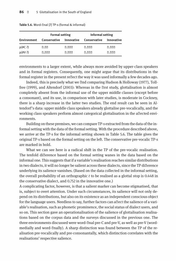
86 | 5 Glottalisation in the South of England
Table 5.6.Word-final [ʔ] TP-s (formal & informal)
Formal setting Informal settingEnvironment Conservative Innovative Conservative Innovative
p(#C∣ʔ) 0.66 0.486 0.572 0.486p(#V∣ʔ) 0.017 0.202 0.103 0.199
environments to a larger extent, while always more avoided by upper-class speakersand in formal registers. Consequently, one might argue that its distributions in theformal register in the present reflect the way it was used informally a few decades ago.
Indeed, this is precisely what we find comparing Hudson & Holloway (1977), Tollfree (1999), and Altendorf (2003): Whereas in the first study, glottalisation is almostcompletely absent from the informal use of the upper middle classes (except beforea consonant), and its use, in comparison with later studies, is moderate in Cockney,there is a sharp increase in the latter two studies. The end result can be seen in Altendorf’s data: upper middle class speakers already glottalise pre-vocalically, and theworking class speakers perform almost categorical glottalisation in the affected environments.
Buildingon thesepremises,we cancompareTP-s extracted from thedata of the informal settingwith the data of the formal setting. With the procedure described above,we arrive at the TP-s for the informal setting shown in Table 5.6. The table gives theoriginal TP-s based on the formal setting on the left. The conservative pre-vocalic TP-sare marked in bold.
What we can see here is a radical shift in the TP of the pre-vocalic realisation.The tenfold difference based on the formal setting wanes in the data based on theinformal one. This suggests that if a variable’s realisation reaches similar distributionsin two dialects, it will no longer be salient across these dialects, since the TP differenceunderlying its salience vanishes. (Based on the data collected in the informal setting,the overall probability of an orthographic t to be realised as a glottal stop is 0.448 inthe conservative dialect, and 0.752 in the innovative one.)A complicating factor, however, is that a salient marker can become stigmatised, thatis, subject to overt attention. Under such circumstances, its salience will not only depend on its distributions, but also on its existence as an independent conscious objectfor the language users. Needless to say, further factors can affect the salience of a variable’s realisation, such as phonetic prominence, the social status of dialect users, andso on. This section gave an operationalisation of the salience of glottalisation realisations based on the corpus data and the surveys discussed in the previous one. Thethree environments discussedwere word-final pre-C and pre-V, aswell as pre-V (word-medially and word-finally). A sharp distinction was found between the TP of the realisation pre-vocalically and pre-consonantally, which distinction correlates with therealisations’ respective salience.

5.3 Concluding remarks | 87
5.3 Concluding remarks
This section used a narrowperspective to look at a dialectal variable, /t/ glottalisationin the South of England. Concentrating on the pattern’s distribution and salience inthe word-final position, I argued that the salience of pre-vocalic glottalisation is dueto the different distributions in the conservative and innovative dialects. The pointof comparison was the pre-consonantal position, where the pattern seems to lacksalience. Salience and distributions were established based on previous studies onthe subject, including an attitude test by Fabricius, and a larger-scale study by Altendorf, as well as based on corpora of upper-middle class and working class speechin the South.
Using corpus data along with results of previous studies, I reached the conclusion that there is a large frequency difference in the salient environment, but not inthe non-salient one. This shows a correlation between the pattern’s transitional probabilities and the pattern’s salience. We can assume, then, that, at least in the word-final position, there is a relationship between probability distributions and the socialevaluation of the variable. Acknowledging the possible effects of the variable’s stigmatisation, we can predict that the same is true for other environments, and that thespread of glottalisation eventually eradicated the difference in distributions, and, consequently, the pattern’s salience. Indeed, this is partly supported by the inexorablespread of glottalisation with respect to environments, registers, and social classes, ascan be witnessed in studies on the phenomenon.
There is one question left unaddressed. I demonstrated that there is a relationship between the salience and the different distributions of the variable in workingclass and upper-middle class speech. I avoided, however, the discussion on the origins of these different distributions, that is, why upper-middle class speakers seemto glottalise to a much lesser extent word-finally before a vowel than their workingclass counterparts, while both speaker groups seem to realise the variable to a similarextent in the same position before a consonant.
This issue is inexorably related to salience itself. Speakers aiming at a higher register or style will avoid pre-vocalic glottalisation, even if inadvertently, because it isa lower prestige marker. Then again, such a statement is not very meaningful, as itonly amounts to an observation of inherent circularity: certain speakers avoid glottalisation in this position, hence we arrive at different distributions, hence it is salient,hence speakers avoid it.
Another factor in the emergence of the difference in distributions, one, that is –luckily for us – independent from the social evaluation of the variable, is the phonology of glottalisation. Pre-consonantal glottalisation is phonetically motivated, as theloss of place of the coronal stop can be a natural consequence of its flanking by thefollowing consonant. In that sense, pre-C glottalisation, if not expected, is hardly surprising. Pre-V glottalisation, however, is different. Its rise can not be motivated that

88 | 5 Glottalisation in the South of England
easily by the pure phonetics, and is likely influenced by the given presence of pre-Cin the language. This is, to an extent, true for word-final pre-V glottalisation, and canbe even more easily observed in the case of word-medial intervocalic glottalisation(the [lɛʔə] ‘letter’ type), where the phonetically motivated lenition pattern is flapping,not glottalisation. Therefore, the different distributions in the twoword-final positionshave something to do with the way glottalised alternants came into existence in thesepositions in the first place. Differences between the perception of various glottalisation patterns in English are noted in Chapter 9.
6 Hiatus resolution in HungarianThe two previous studies showed how one can provide a model of cognitive saliencefor a sociolinguistic variable, given that enough evidence is available on the phoneticrealisation, distribution, and social evaluation of the variants, alongwith informationon the dynamics of the speech community. We saw that there is a trade-off betweenthe amount of data used and the abstraction of the model, both contributing towardsthe validity of the operationalisation of the variable’s sociolinguistic salience in theideal case.
In this chapter, I turn to Hungarian in order to see whether cognitive salience canbe an explanatory factor in the case of phenomena where the available data are morescarce. Due to the time and effort going into the creation of a sociolinguistic corpusit is not surprising that large and encompassing ones are, for most languages, fewand far between. Zséder et al. (2012) propose an alternative to a ‘hand-crafted’ corpusas a possible tool of linguistic variation, namely, web corpora, linguistic resourcescompiled from the publicly available internet traffic in the given language (in our case,Hungarian), in a largely automated manner. The authors argue that the robustness ofsuch corpora, alongwith their accessibility – relying on already availablematerial andcomputationalmethods for the compilation of the corpus –make these excellent toolsin the study of language structure and linguistic variation.
A point relevant to sociolinguistic salience is, of course, that written corpora canbe used – to a certain extent – to assess segmental transitional probabilities as well,thereby allowing the researcher to approximate the distributions of a variant for a language where no corpora have been collected through fieldwork.
In what follows, I look at two patterns of variation in Hungarian. I will argue that,based on available data on speaker attitudes, one is socially salient to the languageusers, while the other one is not. I will use the Hungarian Webcorpus to approximatethe distributions of the respective variants in spoken Hungarian in order to show thatthe reason behind the difference in social salience is cognitive salience: One variableis cognitively salient, which is not true for the other one.
This is a relevant result in the sense that it suggests that the non-salient patternwill never gain social indexation. If the difference had lied exclusively in the extent ofspeaker awareness to the variables, that is, social salience, we could expect both toeventually become social markers.
6.1 BackgroundThe phenomenon under scrutiny, hiatus resolution in Hungarian, is relatively poorlyresearched from the sociolinguistic perspective. Essentially, Educated ColloquialHungarian (ECH), the standard dialect spoken in Budapest and the major cities, has two
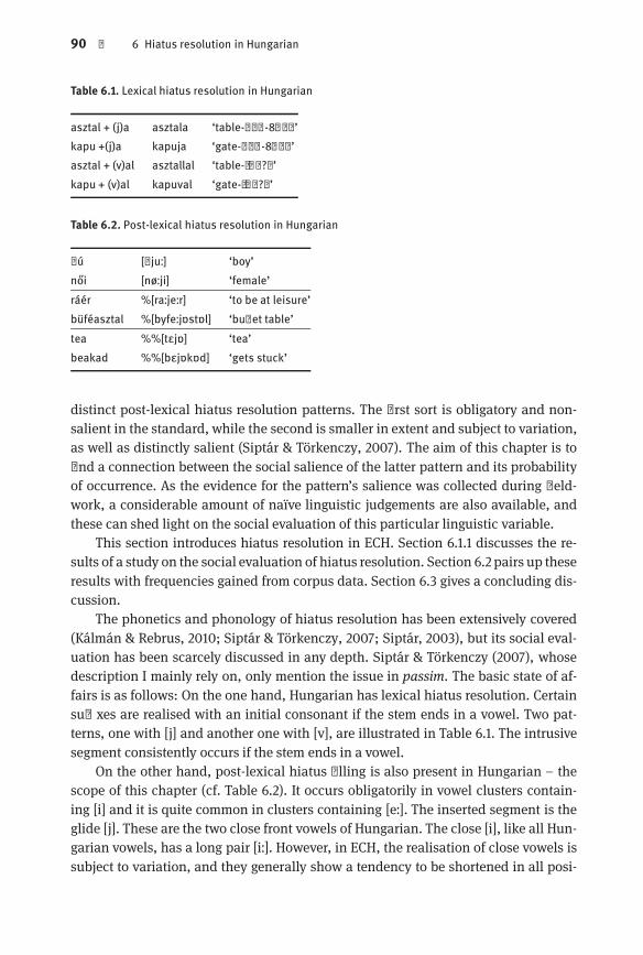
90 | 6 Hiatus resolution in Hungarian
Table 6.1. Lexical hiatus resolution in Hungarian
asztal + (j)a asztala ‘table-3sg-poss’kapu +(j)a kapuja ‘gate-3sg-poss’asztal + (v)al asztallal ‘table-instr’kapu + (v)al kapuval ‘gate-instr’
Table 6.2. Post-lexical hiatus resolution in Hungarian
fiú [fijuː] ‘boy’női [nøːji] ‘female’ráér %[raːjeːr] ‘to be at leisure’büféasztal %[byfeːjɒstɒl] ‘buffet table’tea %%[tɛjɒ] ‘tea’beakad %%[bɛjɒkɒd] ‘gets stuck’
distinct post-lexical hiatus resolution patterns. The first sort is obligatory and non-salient in the standard, while the second is smaller in extent and subject to variation,as well as distinctly salient (Siptár & Törkenczy, 2007). The aim of this chapter is tofind a connection between the social salience of the latter pattern and its probabilityof occurrence. As the evidence for the pattern’s salience was collected during fieldwork, a considerable amount of naïve linguistic judgements are also available, andthese can shed light on the social evaluation of this particular linguistic variable.
This section introduces hiatus resolution in ECH. Section 6.1.1 discusses the results of a study on the social evaluation of hiatus resolution. Section 6.2 pairs up theseresults with frequencies gained from corpus data. Section 6.3 gives a concluding discussion.
The phonetics and phonology of hiatus resolution has been extensively covered(Kálmán & Rebrus, 2010; Siptár & Törkenczy, 2007; Siptár, 2003), but its social evaluation has been scarcely discussed in any depth. Siptár & Törkenczy (2007), whosedescription I mainly rely on, only mention the issue in passim. The basic state of affairs is as follows: On the one hand, Hungarian has lexical hiatus resolution. Certainsuffixes are realised with an initial consonant if the stem ends in a vowel. Two patterns, one with [j] and another one with [v], are illustrated in Table 6.1. The intrusivesegment consistently occurs if the stem ends in a vowel.
On the other hand, post-lexical hiatus filling is also present in Hungarian – thescope of this chapter (cf. Table 6.2). It occurs obligatorily in vowel clusters containing [i] and it is quite common in clusters containing [eː]. The inserted segment is theglide [j]. These are the two close front vowels of Hungarian. The close [i], like all Hungarian vowels, has a long pair [iː]. However, in ECH, the realisation of close vowels issubject to variation, and they generally show a tendency to be shortened in all posi
6.1 Background | 91
tions except the initial syllable. This bears no importance on the present discussion.The short pair of [eː] differs not only quantitatively but also qualitatively, as it is realised as an open mid [ɛ].
Vowel clusters containing [ɛ] but not [i] or [eː] also show hiatus resolution, it is,however, realised less frequently, and, in any case, is subject to variation. There are nodata on the extent of hiatus resolution in the three environments, namely, in clustersinvolving [i], [eː], and [ɛ], respectively, but it is commonly assumed that, in Conservative ECH, hiatus resolution is obligatory in the first, variable in the second, and absentin the third environment. However, as Siptár and Törkenczy note, Innovative ECHdoeshave hiatus resolution in the third environment, although to a limited extent.
I will argue that, compared to the first two environments, hiatus resolution in thethird one is salient for the speakers of ECH. That is, while neither of the hiatus resolution processes in Conservative ECH create salient patterns, the sequences resultingfrom Innovative ECH hiatus resolution are noticeable for language users. We will seethat a simple phonetic explanation is insufficient for the salience of [ɛ] plus [j] patterns, because these are not noticed in any way unless when resulting from hiatusresolution.
I am going to underpin my argument using the results of an attitude test on theperception of the variants of this variable. The test provides empirical evidence onthe pattern’s salience. It is also a valuable resource of naïve linguistic judgements anddescriptionsof the variable. In order to allow the reader to interpret someof these comments in a larger context, we have to briefly overview other phenomena in Hungarianwhich involve j-insertion.
One phenomenon that is directly related to hiatus resolution is that the intensityand duration of the inserted glide can vary. Though again there are no exact data onthis variation, native speakers, to an extent, share a sentiment that an extended glideinserted into a cluster where hiatus resolution is obligatory is a strong substandardfeature. However, it is likely that there is no substantial phonetic difference betweeninserted [j]-s and phonemic [j]-s, a point to which we will return below.
Amore tangible pattern is displayed by the possessive. As noted above, possessiveallomorphy avoids hiatuses: if the stem ends in a vowel, the suffix is -je or -ja. If thestem ends in a sibilant/palatal consonant, however, the occurrence of the glide is subject to variation. This variation, coupled with the fact that the glide-initial allomorphis the productive one, added to recent loanwords, leads to hesitations in possessiveselection, as well as to a general sentiment that there is something going on with [j] inthe possessive (Rácz & Rebrus, 2012).
A third relevant variable is the realisation of the definite article. In standard ECH,it has two forms, a, az, depending on whether the following word starts with a consonant. In certain Transdanubiandialects, definite article allomorphy is also sensitive towhether the previous word ends with a consonant. If it ends with a vowel, the articlehas an initial glide. This is shown in Table 6.3.
92 | 6 Hiatus resolution in Hungarian
Table 6.3. Definite article allomorphy
Standard Dialectal Gloss
V# #V adja az ég adja jaz ég ‘Would to heaven!’V# #C számolja a pénzt számolja ja pénzt ‘she is counting money’C# #C lement a nap lement a nap ‘the sun went down’C# #V finom az alma finom az alma ‘apples are tasty’
As we can see, these processes all involve [j], but are otherwise entirely different:they relate to phonetic realisation of the hiatus filler, the selection of a suffix, and therealisation of the definite article. For the time being, we will go back to the salient andnon-salient forms of hiatus filling, discussed in this section above.
To recap things briefly, in conservative ECH, hiatus resolution is obligatory invowel clusters including [i], and it is variable in clusters with [eː]. In innovative dialects, it is also possible in clusters with [ɛ]. I claimed that the first two hiatus resolution patterns are not salient for ECH speakers, while the latter is. In order to evaluatethis claim, I performed an attitude study with native speakers of ECH.
6.1.1 The perception of hiatus resolution: Methods
The test included ten ECH speakers, five female, fivemale, with amean age of 22. Eightwere from Budapest, and two from the surrounding Pest country. The participantslistened to a recording of 30 sentence pairs, 10 with vowel plus [ɛ] clusters, 10 with[ɛ] plus vowel clusters, and ten control sentences, featuring V[i]/[i]V and V[eː]/[eː]Vequally. The recordings were mono audio waveform files, sampled at 44100Hz. Theparticipants were not paid for the experiment.
The test sentences were read by a trained phonetician, also a native speaker ofECH, oncewith a hiatus filler [j], oncewithout one. The control sentences were all readwitha realisedhiatusfiller. Thebackground informationgiven toparticipantswas thata Hungarian male in his twenties is looking for their help in general linguistic andstylistic issues, as he is going to a job interview in Budapest and is unsure about thequality of his Hungarian. The participants had to evaluate the sentence pairs (with theimplication that the sentences are different) on a Likert-scale from 1 to 10, dependingon whether they found the first or the second sentence better (or they were unsure,etc.). Theparticipants listened to thepairs in a randomorder, both in the sense that theorder of pairswas randomised and that the order of themarked sentence (the onewithhiatus resolution) and the unmarked sentence (the one without it) was randomised:half the pairs had themarked sentence first. The listening test was followed by a smalldiscussion with the participants.

6.1 Background | 93
The experiment has two conditions: (i) whether the marked sentence comes firstor second and (ii) whether the judgements on the test sentences differ from judgements on the control sentences. The hypothesis is that hiatus resolution with [ɛ] is asalient variable that will be rejected, whereas hiatus resolution with [i] and [eː] elicits no listener attitudes. This should show up in condition (i) as a larger score on thescale if the first sentence is marked in the pair and vice versa, and in (ii) as a scoremore divergent from the mean in the case of test sentences versus control sentences,as participants are not expected to show explicit preference for any sentence in a pairof control sentences.
6.1.2 The perception of hiatus resolution: Results
The results show a strong preference for the unmarked pattern in condition (i) andmore divergent scores in condition (ii), which confirms the hypothesis that hiatus resolution in [ɛ]+V clusters is rejected, hence, salient for ECH speakers.
The results were weighted between participants. For condition (i), the resultingscores were modified in such a way that a higher score means a preference for themarked pattern. Condition (ii) is needed in the first place because condition (i) relieson the order of sentences within the pairs. Therefore, the results can be influenced notonly by which sentence wasmarked, but also by the order itself: if the first sentence ismarked, chances are, people become more aware of it. Since condition (ii) comparesall the test sentences with the control sentences, the problem of ordering disappears.
The scores are shown in Figure 6.1 for the first condition and Figure 6.2 for thesecond one. In the Figure 6.1, the first column is the control, the second is where the
●
●●
●●
●
●
●
●
●
●
●
●
●
●
●
●●●●
n.a. no yes
−2−1
01
2
Condition: second sentence marked
Wei
ghte
d sc
ore,
rela
tive
Fig. 6.1.Weighted scores for condition (i)
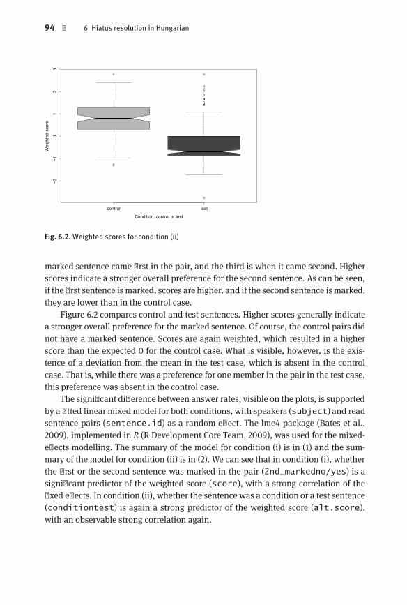
94 | 6 Hiatus resolution in Hungarian
●
●
●
●●
●●●
●
●
●
●
●
●●
●
control test
−2−1
01
23
Condition: control or test
Wei
ghte
d sc
ore
Fig. 6.2.Weighted scores for condition (ii)
marked sentence came first in the pair, and the third is when it came second. Higherscores indicate a stronger overall preference for the second sentence. As can be seen,if the first sentence ismarked, scores are higher, and if the second sentence ismarked,they are lower than in the control case.
Figure 6.2 compares control and test sentences. Higher scores generally indicatea stronger overall preference for the marked sentence. Of course, the control pairs didnot have a marked sentence. Scores are again weighted, which resulted in a higherscore than the expected 0 for the control case. What is visible, however, is the existence of a deviation from the mean in the test case, which is absent in the controlcase. That is, while there was a preference for one member in the pair in the test case,this preference was absent in the control case.
The significant difference between answer rates, visible on the plots, is supportedby a fitted linear mixedmodel for both conditions, with speakers (subject) and readsentence pairs (sentence.id) as a random effect. The lme4 package (Bates et al.,2009), implemented in R (R Development Core Team, 2009), was used for the mixed-effects modelling. The summary of the model for condition (i) is in (1) and the summary of the model for condition (ii) is in (2). We can see that in condition (i), whetherthe first or the second sentence was marked in the pair (2nd_markedno/yes) is asignificant predictor of the weighted score (score), with a strong correlation of thefixed effects. In condition (ii), whether the sentence was a condition or a test sentence(conditiontest) is again a strong predictor of the weighted score (alt.score),with an observable strong correlation again.

6.1 Background | 95
(1) Summary of the model for condition (i)
Linear mixed model fit by REML
Formula: score ~ 2nd_marked + (1 | subject) + (1 | sentence.id)
Data: datAIC BIC logLik deviance REMLdev
749.9 772.1 -368.9 730.1 737.9
Random effects:Groups Name Variance Std.Dev.
sentence.id (Intercept) 0.054274 0.23297
subject (Intercept) 0.000000 0.00000Residual 0.633746 0.79608
Number of obs: 300, groups: sentence.id, 30; subject, 10
Fixed effects:Estimate Std. Error t value
(Intercept) 0.7434 0.1085 6.854
2nd_markedno -0.9542 0.1576 -6.0552nd_markedyes -1.2466 0.1499 -8.318
Correlation of Fixed Effects:(Intr) X2nd_s_mrkdn
2nd_mrkdn -0.688
2nd_mrkdy -0.724 0.498
(2) Summary of the model for condition (ii)
Linear mixed model fit by REML
Formula: alt.score ~ condition + (1 | subject) + (1 | sentence.id)
Data: datAIC BIC logLik deviance REMLdev
749.5 768 -369.7 733.7 739.5
Random effects:Groups Name Variance Std.Dev.
sentence.id (Intercept) 0.065188 0.25532
subject (Intercept) 0.000000 0.00000Residual 0.633746 0.79608
Number of obs: 300, groups: sentence.id, 30; subject, 10
Fixed effects:Estimate Std. Error t value
(Intercept) 0.7434 0.1134 6.556
conditiontest -1.1151 0.1389 -8.030
Correlation of Fixed Effects:
(Intr)conditintst -0.816

96 | 6 Hiatus resolution in Hungarian
In sum, the results confirm speaker awareness of the Innovative hiatus resolution pattern vis-à-vis the Conservative pattern. For a Hungarian linguist, this is hardly surprising, as the pattern is overtly discussed, and some forms like teja are used playfully byspeakers who otherwise eschew Innovative hiatus resolution. It is, however, important to stress that, until now, the pattern’s social evaluation has not been empiricallytested.
6.1.3 Hiatus resolution and naïve linguistic awareness
Each listening session was followed by a short discussion where the participant wasasked to guess what the experiment was about. The comments gained during thesesessions cannot be assessed quantitatively, but shed light on the subjective evaluationof the variable.
First of all, most participants picked up on the fact that there is something goingonwith [j]. Contrary to expectations, not all of themwere able to pinpoint themain difference within the pairs: two participants put emphasis on the intonation differencesthey perceived alongside [j], even though the differences in intonation between thesentences was negligible. One participant did not name [j] at all, even though the participant also showed significant preference for the [j]-less realisation of vowel clusterscontaining [ɛ].
Participants who did mention [j] as a part of the perceived difference varied intheir precision in judging the nature of the difference. Some located the salient hiatuses, and one explicitlymentioned [tɛjɒ] ‘tea’ as an example. Others gave instances ofnon-salient hiatus resolution as an example of the perceived difference, but increasedthe duration and intensity of the intrusive glide. One participant mentioned the non-standard realisation of the definite article, with an initial [j] following V-final words,and another referred to possessive variation, also including [j] (these processes arediscussed in Section 6.1).
The comments show that language users are unable to pin down the variable, despite its salience. Even if they themselves notice the difference, they are not capableof reporting on it. It is generally (though not always) recognised that [j] is the culprit,but the comments invoke other, unrelated phonological, morpho-phonological, andmorphological phenomena, including the non-salient hiatus resolution pattern. Thereason for the latter, I suspect, is the orthography. Intrusive [j]-s are not indicated inthe orthography, whereas, for instance, the (post-vocalically) also predictable possessive suffix is.
To summarise the findings of the attitude study, it confirms the salience of theInnovative hiatus filling pattern, compared to the Conservative one. The participants’comments also show that while speakers are aware of the variable, they are unable todescribe its behaviour accurately.
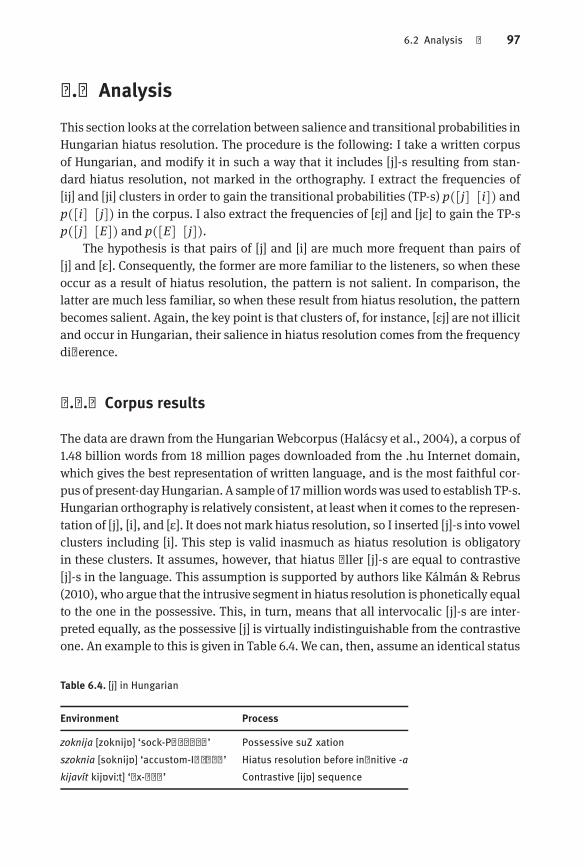
6.2 Analysis | 97
6.2 Analysis
This section looks at the correlation between salience and transitional probabilities inHungarian hiatus resolution. The procedure is the following: I take a written corpusof Hungarian, and modify it in such a way that it includes [j]-s resulting from standard hiatus resolution, not marked in the orthography. I extract the frequencies of[ij] and [ji] clusters in order to gain the transitional probabilities (TP-s) p([j] ∣ [i]) andp([i] ∣ [j]) in the corpus. I also extract the frequencies of [ɛj] and [jɛ] to gain the TP-sp([j] ∣ [E]) and p([E] ∣ [j]).
The hypothesis is that pairs of [j] and [i] are much more frequent than pairs of[j] and [ɛ]. Consequently, the former are more familiar to the listeners, so when theseoccur as a result of hiatus resolution, the pattern is not salient. In comparison, thelatter are much less familiar, so when these result from hiatus resolution, the patternbecomes salient. Again, the key point is that clusters of, for instance, [ɛj] are not illicitand occur in Hungarian, their salience in hiatus resolution comes from the frequencydifference.
6.2.1 Corpus results
The data are drawn from the HungarianWebcorpus (Halácsy et al., 2004), a corpus of1.48 billion words from 18 million pages downloaded from the .hu Internet domain,which gives the best representation of written language, and is the most faithful corpus of present-dayHungarian. A sample of 17millionwordswas used to establish TP-s.Hungarian orthography is relatively consistent, at least when it comes to the representation of [j], [i], and [ɛ]. It does not mark hiatus resolution, so I inserted [j]-s into vowelclusters including [i]. This step is valid inasmuch as hiatus resolution is obligatoryin these clusters. It assumes, however, that hiatus filler [j]-s are equal to contrastive[j]-s in the language. This assumption is supported by authors like Kálmán & Rebrus(2010), who argue that the intrusive segment in hiatus resolution is phonetically equalto the one in the possessive. This, in turn, means that all intervocalic [j]-s are interpreted equally, as the possessive [j] is virtually indistinguishable from the contrastiveone. An example to this is given in Table 6.4.We can, then, assume an identical status
Table 6.4. [j] in Hungarian
Environment Process
zoknija [zoknijɒ] ‘sock-Poss3sg’ Possessive suffixationszoknia [soknijɒ] ‘accustom-Inf3sg’ Hiatus resolution before infinitive -akijavít kijɒviːt] ‘fix-3sg’ Contrastive [ijɒ] sequence

98 | 6 Hiatus resolution in Hungarian
Table 6.5. Conservative ECH
Lexical sequence Hiatus
kijárat [kijaːrɒt] ‘exit’ kiárad [kijaːrɒd] ‘flow-3sg’Tejút [tɜjuːt] ‘Milky Way’ szemleút [sɛmlɛuːt] ‘field trip’
for the [j]-swhich are lexical or arise through hiatus resolution, an issue touched uponin this chapter.
Even if we take the ontology of [j] as granted, the analysis has to cope with another difficulty, the lack of reliable data on hiatus resolution. In Conservative ECH, itis agreed to be obligatory in vowel clusters with [i] and variable in clusters containing [eː]. There are no estimates on Innovative ECH. In order to tackle the scarcity ofthe data, I take up the approach of looking at transitional probabilities in one dialectinstead of comparing two.
This dialect, Conservative Educated Colloquial Hungarian, is assumed to be represented by the Webcorpus. It has obligatory hiatus resolution with [i], but has nonewith [ɛ] (since it is conservative). Nonetheless, it also has lexical instances of vowelclusters with [i]/[ɛ] and [j]. This is illustrated in Table 6.5.
With these presumptions, we can look at the frequency differences of non-salientand salient hiatus resolution in the corpus. The frequency of the relevant string in thecorpus is given in Table 6.6. (Bothword-internal clusters and clusters including awordboundary were included.) The TP-s are given in Table 6.7 (numbers are rounded to thethird decimal place).
The results show that there is a frequency difference of one order of magnitudebetween the TP of [j] following [i] versus that of [j] following [ɛ]. There is no difference,however, when we look at the pattern the other way around, that is, between the TP of[i] following [j] versus [ɛ] following [j]. This asymmetry can be probably blamed on thepossessive suffix, which is -jɛ after vowel-final front vowel stems. The ratios are shownin Table 6.7 and Figure 6.3.
Table 6.6. String frequenciesin the corpus sample
String Frequency
ɛj 103024jɛ 230857ij 480943ji 391069i 4424703j 2367677ɛ 10892098
Table 6.7. TP-s in the corpus sample
Segments Value
p(j∣ɛ) 0.009ɛ∣j 0.098p(j∣i) 0.109p(i∣j) 0.088
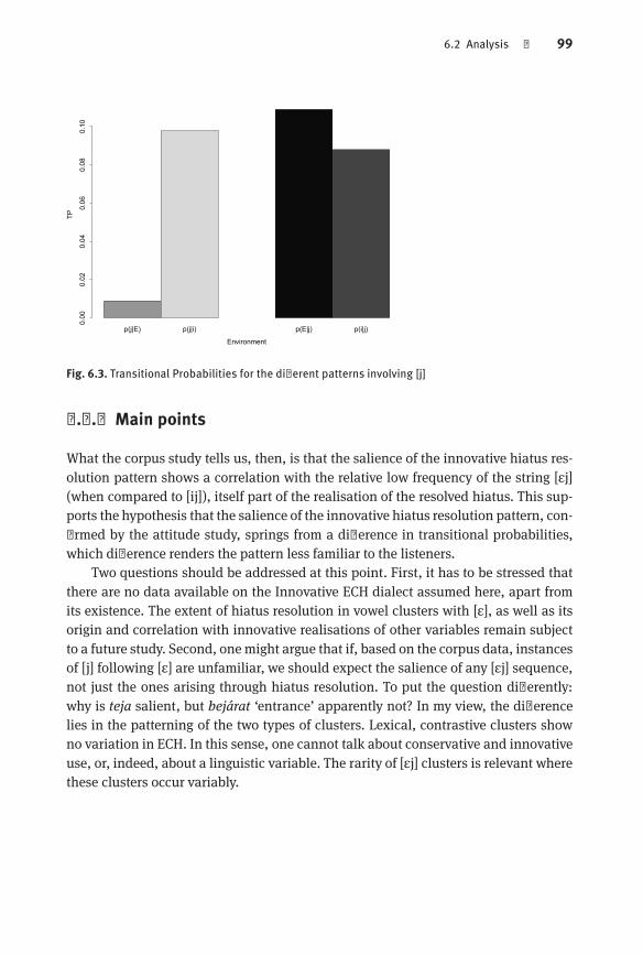
6.2 Analysis | 99
p(j|E) p(j|i) p(E|j) p(i|j)
Environment
TP
0.00
0.02
0.04
0.06
0.08
0.10
Fig. 6.3. Transitional Probabilities for the different patterns involving [j]
6.2.2 Main points
What the corpus study tells us, then, is that the salience of the innovative hiatus resolution pattern shows a correlation with the relative low frequency of the string [ɛj](when compared to [ij]), itself part of the realisation of the resolved hiatus. This supports the hypothesis that the salience of the innovative hiatus resolution pattern, confirmed by the attitude study, springs from a difference in transitional probabilities,which difference renders the pattern less familiar to the listeners.
Two questions should be addressed at this point. First, it has to be stressed thatthere are no data available on the Innovative ECH dialect assumed here, apart fromits existence. The extent of hiatus resolution in vowel clusters with [ɛ], as well as itsorigin and correlation with innovative realisations of other variables remain subjectto a future study. Second, onemight argue that if, based on the corpus data, instancesof [j] following [ɛ] are unfamiliar, we should expect the salience of any [ɛj] sequence,not just the ones arising through hiatus resolution. To put the question differently:why is teja salient, but bejárat ‘entrance’ apparently not? In my view, the differencelies in the patterning of the two types of clusters. Lexical, contrastive clusters showno variation in ECH. In this sense, one cannot talk about conservative and innovativeuse, or, indeed, about a linguistic variable. The rarity of [ɛj] clusters is relevant wherethese clusters occur variably.
100 | 6 Hiatus resolution in Hungarian
6.3 Concluding remarks
This chapter has shown that, in Educated Colloquial Hungarian, a possible reasonfor speaker awareness, or, at least, marked speaker attitudes towards one kind of hiatus resolution but not the other can be linked to the salience of the former, but notthe latter. This difference in being salient, in turn, can be linked up with the different probability of occurrence for the patterns which arise through one type of hiatusresolution as opposed to the other one. Consequently, Hungarian hiatus resolutionis another example of the relationship between salience (as expressed through, forinstance, speaker attitudes) and probability of occurrence.
This study is evidently different from the previous ones in one major respect:whereas, for example, in the case of /t/ glottalisation in the South of England, I compared two dialects in which the variable behaves differently, in the present case, Ilooked at only one dialect, because the amount of available data made a similar comparison impossible. The change in methodology, however, did not influence the mainargument. As shown, salience as a property becomes possible if the extent of useof a variable in one dialect is notably different from this extent in another dialect.If we look at the problem this way, we can say that any variability in a dialect is apossible ‘entry point’ of social evaluation, though not a necessary one. Indeed, thisonly amounts up to saying that linguistic variables carry social indexation, whichshould not come as a shock. What should be stressed, however, is that the interactionbetween salience and distributions can be meaningfully operationalised even whenwe build on data only from one dialect.
A shared trait with the glottalisation study, however, is the problem concerningthe origin of the difference in distributions in the two dialects. The reason why Conservative ECH speakers – as well as upper-middle class speakers from the South ofEngland – notice a variable is that it is realised to a different extent in a dialect dissimilar to their own. In the glottalisation chapter I hinted at a possible explanationfor the precedence of the non-salient variable over the salient one, namely, phoneticgrounding (or the absence thereof). Here, we can take a similar note.
The reasonwhy hiatus resolution in vowel clusters with [i] goes unnoticed inHungarian is that it exhibits no variation. The reason for the absence of variation, however,is probably the phonetic grounding of hiatus resolutionwith [j] in these environments,which grounding is absent in clusters with [ɛ]. What follows is that the latter is muchless susceptible of developing naturally. The consequent priority of the phoneticallygrounded hiatus resolution pattern over the ungrounded one paves the way for thelatter’s salience.

7 Derhoticisation in GlasgowIn the previous chapters, I argued for a straightforward, segmental approach to socialmarkers. If the difference in the realisations of a variable creates differences in thesegmental distributions in two related dialects – in the previous examples, a conservative normdialect and an innovative dialect – speakers become awareof the segmental difference, and, consequently, the social connotations of variable use. This view iscurbed in the sense that it can only apply in cases where we can posit abstract segmental units and differences in variable realisation resulting in differences in the segmental distributions, that is, the transitional probabilities of the segments. As such,the concept of salience only has a bearing on certain consonantal variables. We do expect these variables, however, to meet our expectations and to be sociolinguisticallysalient when the requirements for segmental distributions hold.
If a consonantal variable shows different transitional probabilities in two relateddialects, andyet fails to carry social indexation, the state of affairs becomesmore complicated. Certainly, difference in distributions is not the single and necessary requirement for sociolinguistic salience. Then again, such a case should not be brushed offthe table saying that it is an unfortunate, though legitimate, exception to the rule. It ismuchmore useful to look at the variable’s larger context and ask the questionwhetherthe language system in which the variable is defined has an effect on speaker awareness, and if so, how.
The last case study reverses the argument in a way and proposes that the lack ofsocial salience can be, in certain cases, linked to a lack of cognitive salience, that is,to a lack of surprisal in the distributions.
7.1 Background
This chapter has a look at derhoticisation, the vocalisation of coda /r/ in the UrbanScots dialects ofGlasgow. Iwill argue that, basedonavailabledata, this variable seemsto carry no social indexation, despite the fact that, at first glance it meets the requirements for sociolinguistic salience: It relates to differences in segmental distributionsand shows clear social stratification. I will go on to claim that the apparent absence ofspeaker awareness is due to the vast extent of variability inherent to derhoticisation,and the behaviour of /r/ in Glasgow Scots in general.
The first part of this chapter reviews available research on the pattern, along withthe conclusions previous researchers have drawn from the data. In the second part ofthe chapter, Section 7.2, I test whether we would expect the loss of coda /r/ as sociallysalient, and look at the possible explanations available if it proves not to be salient atall.

102 | 7 Derhoticisation in Glasgow
In Section 7.1.1, I discuss the general problem tackled in the chapter, namely, theexistence of indicators, cases where social stratification does not go with speakerawareness, and the consequences for a segmentally based definition of salience. Section 7.1.2 gives the concrete example, derhoticisation, or the loss of coda /r/ inGlasgowand other Scottish English dialects, and describes available data in detail to show thefullest scale of the variation and relevant factors of this change. Section 7.1.5 givesan interim summary. Based on the conclusions of this summary, Section 7.2.1 buildsa comparative scale of distributions based on data from the Fred corpus, in orderto show that phonetical gradience will lead to large variation, which, in turn, willbereave the variable of salience. Section 7.3 provides a general discussion.
7.1.1 Social stratification and social awareness
The viewmaintained throughout this book is that language change which affects segmental distributions in an unevenway in two related dialects will possibly come to theattention of speakers. Speaker attention does not necessarily involve stigmatisationand other forms of meta-awareness (such as the ability to imitate an accent). However, it goes together with style shifting, the preference of a conservative variant ina formal setting, and explicit attitudes towards speakers using a particular variant.Style shifting does not exclusively happen in this direction, and speaker attitudes cango beyond being simple negative or positive. That notwithstanding, the presence ofstyle shifting or contoured speaker attitudes can be relatively easily ascertained andare reliable indices of speaker awareness.
Social stratification and speaker awareness of a variable should go hand in hand,somuch so that, for socially stratifiedvariables, the absenceof sociolinguistic salienceis more the exception than the rule. One classic example is Labov’s New York Department Store study (Labov, 1972b), which goes so far as to conflate social stratificationand style shifting in collecting data from employees of stores favoured by a clientele of different social backgrounds. Labov’s implicit assumption is that, in case ofthe variable under his scrutiny, (rV), the vocalisation of coda /r/, both social stratification and sociolinguistic salience will be a factor: Any employee of a store of highstanding is both more likely to have a better social status and tend to speak in a more‘sophisticated’ manner with costumers. (During the course of this chapter we will beconfronted with another variable related to /r/, namely, (r), the variable realisation ofcoda /r/, i.e. the variation in its realisation, not whether it is there or not.)
His Lower East Side study (Labov, 1966/2006) shows that such behaviour is notlimited to department store employees: the variable (rV) shows the most fine-grainedcorrelation with social status in the community, and the responses to it betray clearattitudes towards its use in the matched guise tests: his subjects associate a largerextent of coda /r/ realisation with a higher socio-economic standing.
7.1 Background | 103
Such a response is expected if we accept the difference in segmental distributionsas a source of salience. As I will show in section 7.2.1, any shift in the realisation ofcoda /r/ causes considerable changes in the distributions of vowels followed by [r] aswell as [r] preceding consonants: to put it very simply, both of these are fairly rare innon-rhotic dialects of English, and relatively common in rhotic ones.
This approach is warranted when one considers Labov’s own explanation of thelanguage change resulting in the different coda [r] ratios in the Lower East Side, and inNew York City in general. He argues that an external norm, that of other rhotic AmericanEnglish dialects, had been introduced inNewYork City, whichwas adopted first bythe upper social classes, and is pervading the language system. Labov regards rhoticisation in New York City as a classic change from above, that is, a change that happensabove the threshold of consciousness. He admits that the term is somewhat unfortunate, even more so because, in this particular case, it coincides with another verticalmovement: the introduction of the norm by the upper social classes, and its movingdownwards to be adopted by the lower ones. To keep the two terms separate, I willrefer to a change that starts at the higher end of the social ladder, and is proceedingdownwards, as top-down. A change that starts in a social group other than the elite,and typically in the working class, I will call bottom-up.
Changes from above, that is, salient changes do not necessarily proceed top-down. The glottalisation of /t/, discussed in Chapter 5, is an excellent example. Inthe South-East of England it started as a substandard class feature (if we ignore, fora moment, its long and turbulent history). Bottom-up spreading is a characteristicof Labov’s change from below. According to Labov (1966/2006), changes from belowhappen below the threshold of speaker consciousness, and all his examples originatein a lower socio-economic class. One difference, then, between glottalisation and thisnotion of a change from below is that while a change from below is supposed to proceed without any speaker awareness, glottalisation quickly became a characteristicclass feature in England, leading some to claim it as a defining feature of the emergingstandard in the South, Estuary English (Rosewarne, 1984). In this sense, /t/ glottalisation is a bottom-up change, starting below and climbing the social ladder, but, inits later stages, certainly a change from above.
This leaves us with a fourfold typology. Changes from above proceed in away thatis conscious to the speakers, while changes from below remain unnoticed. Top-downchanges are linguistic innovations starting at the top of the social scale, and are heldas a norm for the rest of the community. In contrast, bottom-up changes start loweron the social scale. (One should note that this typology assumes a view of languagechange climbing up and down on a ladder. Details beyond classic class structure areevaded in this chapter, but are taken into consideration in Chapter 9.)
We can probably rest assured that a top-down adaption of a new linguistic normwill be a change from above, a salient change, resulting in style shifting as well as social stratification. Amuchmore interesting question is whether all bottom-up changesendupbeing salient like glottalisation did. Both Labov (1966/2006) and Trudgill (1974)
104 | 7 Derhoticisation in Glasgow
list variables which carry no social indexation, that is, are only indicators, not markers. Clearly, speaker awareness also depends on other factors, such as the extent andspeed of the change in question (as well as its relation to the local norm system). Thedecisive factor, as argued in this book, is salience, emergent from the different distributions of the realisations of the variable in question – the forms affected by languagechange. If, in two related dialects, the difference between the realisations entails differences in the segmental distributions of these dialects, the variable has a chance tobe picked up by listeners and become a social marker. What this means, in turn, isthat quite a number of consonantal variables should be able to carry social indexation, (rV), coda /r/ vocalisation, being a prime example.
The reader should note that this discussion builds on the premise that all linguistic variation is connected to language change, which is not true in all cases (cf. Chapter 9).
As long as it shows social stratification, coda /r/ vocalisation should be an excellent candidate for a linguistic marker – all the more awkward for a theory of salienceif it does not prove to be so in a particular case. The rest of the chapter discusses sucha case, the emergence of a new urban working-class dialect of Glaswegian. Coda /r/vocalisation seems to be an indicator of this dialect, as much as it shows clear socialstratification in Glasgow, but it looks as if speaker awareness were absent.
I argued previously that differences in segmental distributions do not necessarilylead to sociolinguistic salience. Yet, instead of filing Glasgow /r/ as an apparent counterexample, Iwill try to look into its general context to answer the questionwhy it doesnot carry social indexation, though it could – at least based on expectations couchedin this theory.
7.1.2 Derhoticisation in Glasgow
The vocalisation of coda /r/, or derhoticisation, is not a newphenomenon in Scotland.Scottish English (and Scots) are traditionally regarded as rhotic, that is, consistentlyrealising post-vocalic /r/ in words like car and card. The most conservative view on/r/ in Scottish English dialects is that it is realised as an alveolar trill, a sound realisedby vibrations between the tip of the tongue and the alveolar ridge of the palate. Thestandard realisation, however, is commonly regarded to be a retroflex approximant, asound realised by a narrow constriction of the tongue body or tongue tip behind thealveolar ridge (Wells, 1982). As wewill see, this traditionalmiddle-class variant is nowcontested by a new one, typical of working-classmale adolescents, andworking-classspeakers in general. This variant is the alveolar tap, a single constriction created bythe tip of the tongue and the alveolar ridge. These two are not the only possible, or,indeed, prevalent realisations of /r/ in Scotland, as both central approximants and, toan extent, uvular approximants and trills are to be found (Stuart-Smith, 2003).
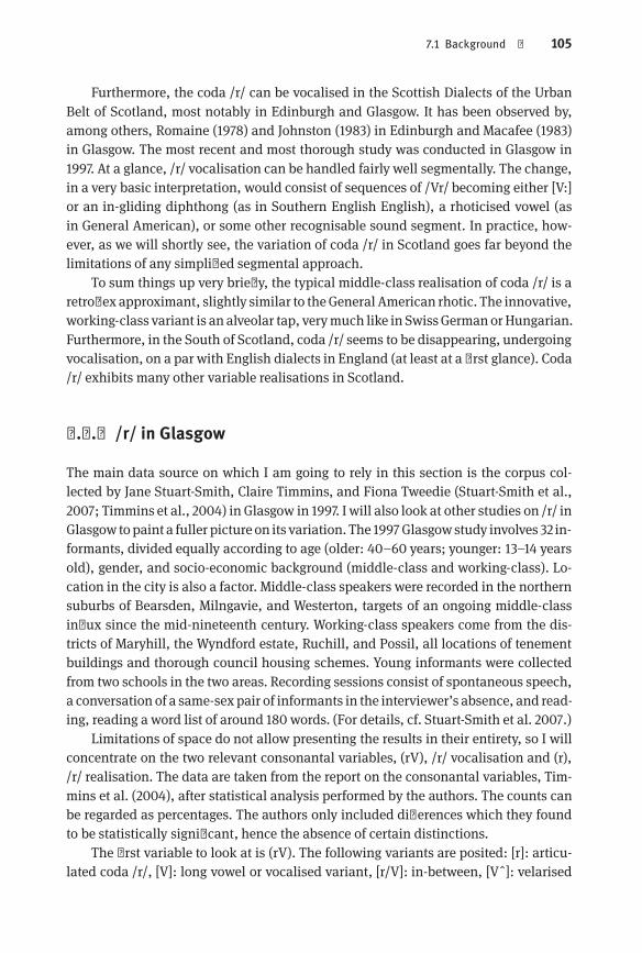
7.1 Background | 105
Furthermore, the coda /r/ can be vocalised in the Scottish Dialects of the UrbanBelt of Scotland, most notably in Edinburgh and Glasgow. It has been observed by,among others, Romaine (1978) and Johnston (1983) in Edinburgh and Macafee (1983)in Glasgow. The most recent and most thorough study was conducted in Glasgow in1997. At a glance, /r/ vocalisation can be handled fairly well segmentally. The change,in a very basic interpretation, would consist of sequences of /Vr/ becoming either [V:]or an in-gliding diphthong (as in Southern English English), a rhoticised vowel (asin General American), or some other recognisable sound segment. In practice, however, as we will shortly see, the variation of coda /r/ in Scotland goes far beyond thelimitations of any simplified segmental approach.
To sum things up very briefly, the typical middle-class realisation of coda /r/ is aretroflex approximant, slightly similar to theGeneral American rhotic. The innovative,working-class variant is an alveolar tap, verymuch like in SwissGermanorHungarian.Furthermore, in the South of Scotland, coda /r/ seems to be disappearing, undergoingvocalisation, on a par with English dialects in England (at least at a first glance). Coda/r/ exhibits many other variable realisations in Scotland.
7.1.3 /r/ in Glasgow
The main data source on which I am going to rely in this section is the corpus collected by Jane Stuart-Smith, Claire Timmins, and Fiona Tweedie (Stuart-Smith et al.,2007; Timmins et al., 2004) in Glasgow in 1997. I will also look at other studies on /r/ inGlasgow topaint a fuller picture on its variation. The 1997Glasgowstudy involves 32 informants, divided equally according to age (older: 40–60 years; younger: 13–14 yearsold), gender, and socio-economic background (middle-class and working-class). Location in the city is also a factor. Middle-class speakers were recorded in the northernsuburbs of Bearsden, Milngavie, and Westerton, targets of an ongoing middle-classinflux since the mid-nineteenth century. Working-class speakers come from the districts of Maryhill, the Wyndford estate, Ruchill, and Possil, all locations of tenementbuildings and thorough council housing schemes. Young informants were collectedfrom two schools in the two areas. Recording sessions consist of spontaneous speech,a conversation of a same-sex pair of informants in the interviewer’s absence, and reading, reading a word list of around 180 words. (For details, cf. Stuart-Smith et al. 2007.)
Limitations of space do not allow presenting the results in their entirety, so I willconcentrate on the two relevant consonantal variables, (rV), /r/ vocalisation and (r),/r/ realisation. The data are taken from the report on the consonantal variables, Timmins et al. (2004), after statistical analysis performed by the authors. The counts canbe regarded as percentages. The authors only included differences which they foundto be statistically significant, hence the absence of certain distinctions.
The first variable to look at is (rV). The following variants are posited: [r]: articulated coda /r/, [V]: long vowel or vocalised variant, [r/V]: in-between, [Vˆ]: velarised
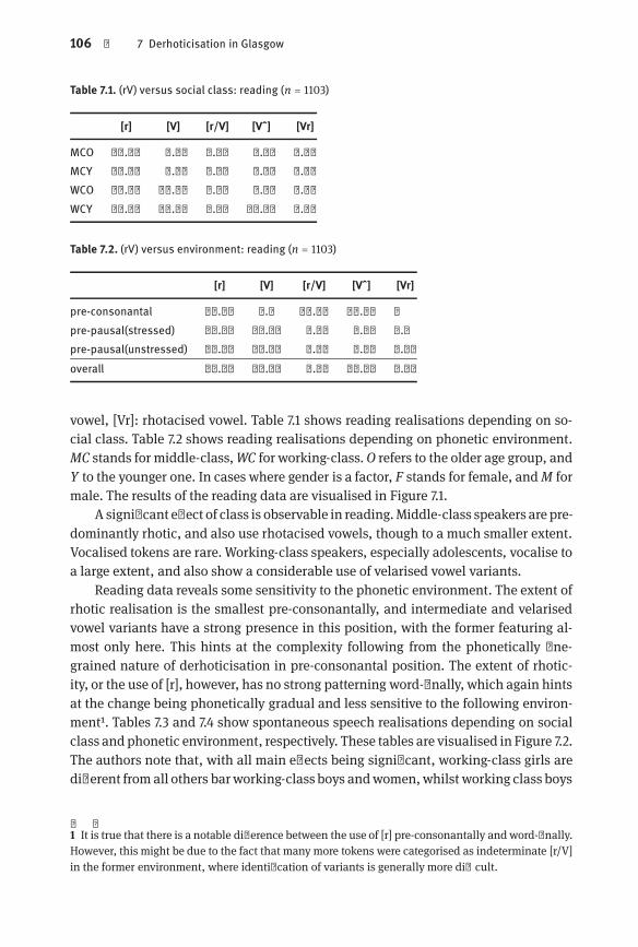
106 | 7 Derhoticisation in Glasgow
Table 7.1. (rV) versus social class: reading (n = 1103)
[r] [V] [r/V] [Vˆ] [Vr]
MCO 88.21 1.43 0.36 1.43 8.57MCY 81.41 6.32 0.00 5.58 6.69WCO 62.91 17.45 2.55 9.82 7.27WCY 17.56 50.54 2.15 25.81 3.94
Table 7.2. (rV) versus environment: reading (n = 1103)
[r] [V] [r/V] [Vˆ] [Vr]
pre-consonantal 51.57 9.1 19.08 20.24 0pre-pausal(stressed) 69.84 19.94 0.78 9.18 0.2pre-pausal(unstressed) 63.54 26.56 1.56 6.25 2.08overall 61.65 18.53 7.14 11.89 0.76
vowel, [Vr]: rhotacised vowel. Table 7.1 shows reading realisations depending on social class. Table 7.2 shows reading realisations depending on phonetic environment.MC stands for middle-class,WC for working-class.O refers to the older age group, andY to the younger one. In cases where gender is a factor, F stands for female, andM formale. The results of the reading data are visualised in Figure 7.1.
A significant effect of class is observable in reading.Middle-class speakers are predominantly rhotic, and also use rhotacised vowels, though to a much smaller extent.Vocalised tokens are rare. Working-class speakers, especially adolescents, vocalise toa large extent, and also show a considerable use of velarised vowel variants.
Reading data reveals some sensitivity to the phonetic environment. The extent ofrhotic realisation is the smallest pre-consonantally, and intermediate and velarisedvowel variants have a strong presence in this position, with the former featuring almost only here. This hints at the complexity following from the phonetically fine-grained nature of derhoticisation in pre-consonantal position. The extent of rhoticity, or the use of [r], however, has no strong patterning word-finally, which again hintsat the change being phonetically gradual and less sensitive to the following environment¹. Tables 7.3 and 7.4 show spontaneous speech realisations depending on socialclass andphonetic environment, respectively. These tables are visualised in Figure 7.2.The authors note that, with all main effects being significant, working-class girls aredifferent from all others barworking-class boys andwomen,whilst working class boys
||1 It is true that there is a notable difference between the use of [r] pre-consonantally and word-finally.However, this might be due to the fact that many more tokens were categorised as indeterminate [r/V]in the former environment, where identification of variants is generally more difficult.

7.1 Background | 107
MCO
MCY
WCO
WCY
Percentages
Clas
s
0 20 40 60 80 100
[r]
[V]
[r/V]
[V^]
[Vr]
pre−
Cpr
e−pa
use
(str)
pre−
paus
e (u
nstr)
Percentages
Envir
onm
ent
0 20 40 60 80 100
[r]
[V]
[r/V]
[V^]
[Vr]
Fig. 7.1. Derhoticisation versus social class and environment: reading (n = 1103)
are polarised frommiddle-classmenand girls.Wemight observe that readingpatternsare retained in the sense that middle-class speakers are mostly rhotic with working-class speakers and especially working-class adolescents vocalising much more. One
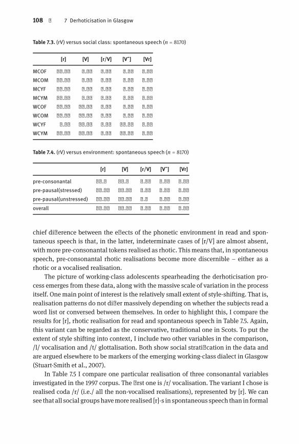
108 | 7 Derhoticisation in Glasgow
Table 7.3. (rV) versus social class: spontaneous speech (n = 8170)
[r] [V] [r/V] [Vˆ] [Vr]
MCOF 94.33 4.12 0.14 0.07 1.35MCOM 92.02 3.71 0.00 2.23 2.04MCYF 93.03 2.92 0.16 0.00 3.89MCYM 89.39 4.22 0.22 4.65 1.52WCOF 69.07 22.45 0.86 2.42 5.20WCOM 75.38 12.94 0.51 6.85 4.32WCYF 5.82 76.33 1.50 15.15 1.20WCYM 22.13 50.50 2.21 17.51 7.65
Table 7.4. (rV) versus environment: spontaneous speech (n = 8170)
[r] [V] [r/V] [Vˆ] [Vr]
pre-consonantal 64.6 19.5 0.56 7.69 7.65pre-pausal(stressed) 70.71 21.45 0.87 5.91 1.06pre-pausal(unstressed) 67.84 27.13 0.9 3.34 0.79overall 67.72 22.69 0.78 5.65 3.17
chief difference between the effects of the phonetic environment in read and spontaneous speech is that, in the latter, indeterminate cases of [r/V] are almost absent,withmore pre-consonantal tokens realised as rhotic. Thismeans that, in spontaneousspeech, pre-consonantal rhotic realisations become more discernible – either as arhotic or a vocalised realisation.
The picture of working-class adolescents spearheading the derhoticisation process emerges from these data, along with the massive scale of variation in the processitself. Onemain point of interest is the relatively small extent of style-shifting. That is,realisation patterns do not differ massively depending on whether the subjects read aword list or conversed between themselves. In order to highlight this, I compare theresults for [r], rhotic realisation for read and spontaneous speech in Table 7.5. Again,this variant can be regarded as the conservative, traditional one in Scots. To put theextent of style shifting into context, I include two other variables in the comparison,/l/ vocalisation and /t/ glottalisation. Both show social stratification in the data andare argued elsewhere to be markers of the emerging working-class dialect in Glasgow(Stuart-Smith et al., 2007).
In Table 7.5 I compare one particular realisation of three consonantal variablesinvestigated in the 1997 corpus. The first one is /r/ vocalisation. The variant I chose isrealised coda /r/ (i.e./ all the non-vocalised realisations), represented by [r]. We cansee that all social groupshavemore realised [r]-s in spontaneous speech than in formal
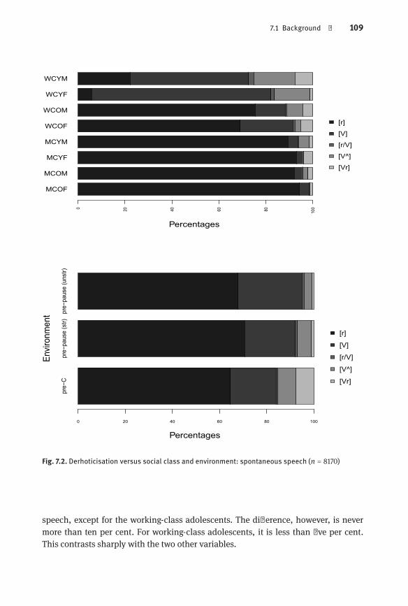
7.1 Background | 109
MCOF
MCOM
MCYF
MCYM
WCOF
WCOM
WCYF
WCYM
Percentages
0 20 40 60 80 100
[r]
[V]
[r/V]
[V^]
[Vr]
pre−
Cpr
e−pa
use
(str)
pre−
paus
e (u
nstr)
Percentages
Envir
onm
ent
0 20 40 60 80 100
[r]
[V]
[r/V]
[V^]
[Vr]
Fig. 7.2. Derhoticisation versus social class and environment: spontaneous speech (n = 8170)
speech, except for the working-class adolescents. The difference, however, is nevermore than ten per cent. For working-class adolescents, it is less than five per cent.This contrasts sharply with the two other variables.

110 | 7 Derhoticisation in Glasgow
Table 7.5. Style shifting examples in the 1997 corpus ((rV) RS n = 1103, SS n = 8170; (l) RS n = 656,SS n = 3420; (t) RS n = 1212, SS n = 2385)
(rvoc):[r] (l):[V] (t):[ʔ]Read S Spont S Read S Spont S Read S Spont S
MCO 88.21 93.17 13.69 0.10 0.7356.56
MCY 81.41 91.21 13.94 0.00 4.65WCO 62.91 72.23 12.05 0.42 6.91
92.47WCY 17.56 13.98 47.13 8.83 76.32
The second one is /l/ vocalisation. The variant shown here is [V], vocalised coda/l/. We can see that middle-class speakers and working-class adolescents do not useit to a large extent in reading in the first place, and completely avoid it in spontaneousspeech. The one exception is again the working-class adolescent group. They use thevocalised variant five times more often in reading than in spontaneous speech. Thismight come as a surprise given the fact that we expect the reverse: avoidance of theinnovative vocalised variant in the more formal reading setting. Stuart-Smith et al.(2007), however, make the point that, as a strongmarker of working-class identity, vocalised /l/ might be exaggerated in the reading list. In any case, the presence of styleshifting in any direction sharply indicates the marker status of this variable. With /t/glottalisation,we seemiddle-class andolderworking-class speakers strongly avoidingthe glottal stop variant [ʔ] in reading, even though the latter group uses it overwhelmingly in spontaneous speech. (The two data points in the last column indicate thatthere is no significant difference in age in the realisation of this variant.) Working-class adolescents also show style-shifting.
Even ifwe think that style shifting is insufficient evidence on social awareness to aparticular variable, it is still striking that coda /r/ realisation shows it much less thanthe other two, all the more since coda /r/ realisation is a textbook example of bothsocial stratification of and social awareness to linguistic variation. One could put forward that derhoticisation in Glasgow, as opposed to ’rhoticisation’ in New York City,evades speaker attention precisely because it fits Labov’s description of a change frombelow: it starts lower on the social scale and proceeds gradually, as an articulatorylenition dependent on the phonetic environment and showing massive variation. Incomparison, inNewYorkCity,wehave the caseof a change fromabove, the almost conscious adoption of an external norm by the upper-middle-classes. Therefore, thoughthe social stratification of coda /r/ realisation is fairly similar in the two cases, withpeople higher on the socio-economic speakingmore rhotic, the comparison of the twolanguage settings is misleading. (Though, it has to be said, the situation is differentwith age: in Glasgow, older speakers tend to be more rhotic, which is the other wayaround in the New York City case.)

7.1 Background | 111
This argument is refuted by the presence of massive style shifting with the othervariables, two of them exemplified above. These variables also seem to participate incarving out a new working-class identity in Glasgow, but all of them start low on thesocial scale, andnot all of them canbe regarded as the conscious adoption of an external norm: Glasgow is the hometown of /t/ glottalisation, and while both this variableand /l/ vocalisation might be influenced by emergent working-class norms elsewherein Britain, they clearly originate in articulatory reduction. Researchers do not agreecompletely on the extent of the influence English working-class standards onGlasgowworking-class speech. One would not want to arbiter on this issue here, but it is certainly true that Stuart-Smith et al. (2007) convincingly argue against blaming languagechange in Glasgow on English English influence (for instance, since the English English standard is non-rhotic, wewould expect conscious adoption by themiddle-classspeakers, and yet the reverse is happening). What ismore, there are other examples ofbottom-up changes becoming social markers, one extensively discussed in this bookbeing /t/ glottalisation in England.
In sum, this discussion brings us back to the distinction between changes fromabove/below and top-down/bottom-up changes. While the two concepts are not completely orthogonal – top-down changes are likely to be always changes from above,innovations salient to the speakers – a bottom-up change may not remain below thethreshold of speaker awareness.
What follows is that the cause for the absence of style shifting in /r/ vocalisationinGlasgow has to be sought elsewhere. Thiswork, of course, argues that the reason fora variable’s salience is not the history or social frameof the change but rather the phonetic/phonological distributions this change affects.Wewill look atmore evidence onthe (absence of) social evaluation of /r/ in Glasgow. But before we do so, we have topay attention to another of the factors that might influence it, namely (r), variation in/r/ realisation.
Stuart-Smith and her colleagues only look at the variation of the realisation of/r/ in the first ten per cent of the conversations in the spontaneous speech registerof the 1997 corpus, due to the large frequency of the variable in speech. Social classand gender, but not phonetic environment is included as factors. They define thefollowing variant categories: [r]: central approximants, [R]: retroflex approximants,[rt]: mainly voiced alveolar taps, [Rt]: retroflex taps, [Ru]: voiced uvular fricative, [rtt]:voiced alveolar trill, [V]: vocalised variants (discussed above), [m]: miscellaneous.Table 7.6 shows the distributions of these variants in reading.
Table 7.6 re-instates a known fact about Scots dialects, namely, that retroflex approximants are typical inmiddle-classuse,with taps beingmore common in theworking-class (Wells, 1982). Central approximants are used, to an extent, by all speakers.The table also shows the extent of /r/ vocalisation, stronger in the case of working-class speakers, and, specifically, working-class adolescents.
Table 7.7 shows (r) in spontaneous speech. Older working-class speakers use theretroflex variant to a much larger extent in spontaneous speech than in reading, and
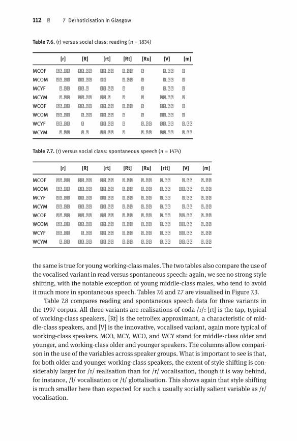
112 | 7 Derhoticisation in Glasgow
Table 7.6. (r) versus social class: reading (n = 1834)
[r] [R] [rt] [Rt] [Ru] [V] [m]
MCOF 13.42 58.87 21.64 0.87 0 5.19 0MCOM 11.25 44.15 29 7.36 0 8.22 0MCYF 6.64 64.6 23.45 0 0 5.31 0MCYM 5.17 41.38 30.6 0 0 22.84 0WCOF 13.85 20.78 44.59 4.76 0 16.02 0WCOM 12.61 0.43 60.87 0 0 26.09 0WCYF 12.66 0 29.69 0 0.44 56.33 0.87WCYM 7.92 2.2 37.44 0 0.44 51.54 0.44
Table 7.7. (r) versus social class: spontaneous speech (n = 1474)
[r] [R] [rt] [Rt] [Ru] [rtt] [V] [m]
MCOF 23.10 52.71 21.66 0.00 0.00 0.00 2.53 0.00MCOM 12.37 64.21 10.37 0.00 0.00 0.00 13.04 0.00MCYF 13.71 60.48 22.58 0.00 0.00 0.00 3.23 0.00MCYM 14.71 52.21 28.68 0.00 0.00 0.00 4.41 0.00WCOF 11.00 39.23 26.79 2.39 0.00 0.00 20.57 0.00WCOM 18.39 44.44 23.75 0.00 0.00 1.15 11.88 0.38WCYF 14.84 4.52 20.00 0.00 0.00 0.00 60.00 0.65WCYM 2.17 19.57 28.26 0.00 2.17 0.00 45.65 2.17
the same is true for youngworking-classmales. The two tables also compare the use ofthe vocalised variant in read versus spontaneous speech: again,we see no strong styleshifting, with the notable exception of young middle-class males, who tend to avoidit much more in spontaneous speech. Tables 7.6 and 7.7 are visualised in Figure 7.3.
Table 7.8 compares reading and spontaneous speech data for three variants inthe 1997 corpus. All three variants are realisations of coda /r/: [rt] is the tap, typicalof working-class speakers, [Rt] is the retroflex approximant, a characteristic of middle-class speakers, and [V] is the innovative, vocalised variant, again more typical ofworking-class speakers. MCO, MCY, WCO, and WCY stand for middle-class older andyounger, andworking-class older and younger speakers. The columns allow comparison in the use of the variables across speaker groups. What is important to see is that,for both older and younger working-class speakers, the extent of style shifting is considerably larger for /r/ realisation than for /r/ vocalisation, though it is way behind,for instance, /l/ vocalisation or /t/ glottalisation. This shows again that style shiftingis much smaller here than expected for such a usually socially salient variable as /r/vocalisation.

7.1 Background | 113
MCOF
MCOM
MCYF
MCYM
WCOF
WCOM
WCYF
WCYM
Percentages
0 20 40 60 80 100
[r]
[R]
[rt]
[Rt]
[Ru]
[V]
[m]
MCOF
MCOM
MCYF
MCYM
WCOF
WCOM
WCYF
WCYM
Percentages
0 20 40 60 80 100
[r]
[R]
[rt]
[Rt]
[Ru]
[V]
[m]
Fig. 7.3. (rV) versus social class: reading and spontaneous speech
Two strong patterns are observable in the /r/ realisation data. First, /r/ realisation,though in no simple way, is socially stratified, with middle-class speakers leaning towards the retroflex variant, and working-class ones towards the flap. This is accompanied by a fair amount of style-shifting, especially with older middle-class speakers,
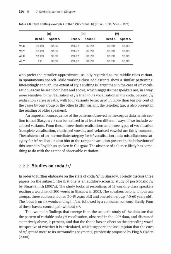
114 | 7 Derhoticisation in Glasgow
Table 7.8. Style shifting examples in the 1997 corpus: (r) (RS n = 1834, SS n = 1474)
[rt] [Rt] [V]Read S Spont S Read S Spont S Read S Spont S
MCO 51.51 58.46 25.32 16.02 88.21 93.17MCY 52.99 56.34 27.03 25.63 81.41 91.21WCO 21.21 41.84 52.73 25.27 62.91 72.23WCY 1.1 12.05 33.57 24.13 17.56 13.98
who prefer the retroflex approximant, usually regarded as the middle class variant,in spontaneous speech. Male working-class adolescents show a similar patterning.Interestingly enough, the extent of style shifting is larger than in the case of /r/ vocalisation, as canbe seen both here and above, which suggests that speakers are, in away,more sensitive to the realisation of /r/ than to its vocalisation in the coda. Second, /r/realisation varies greatly, with four variants being used in more than ten per cent ofthe cases by one group or the other (a fifth variant, the retroflex tap, is also present inthe reading of older speakers).
An important consequence of the patterns observed in the corpus data in this section is that Glasgow /r/ can be realised in at least ten different ways, if we include vocalised variants. From these, three rhotic realisations and three types of vocalisation(complete vocalisation, rhoticised vowels, and velarised vowels) are fairly common.The existence of an intermediate category for /r/ vocalisation and amiscellaneous category for /r/ realisation also hint at the rampant variation present in the behaviour ofthis sound in English as spoken in Glasgow. The absence of salience likely has something to do with the extent of observable variation.
7.1.4 Studies on coda /r/
In order to further elaborate on the state of coda /r/ in Glasgow, I briefly discuss threepapers on the subject. The first one is an auditory-acoustic study of postvocalic /r/by Stuart-Smith (2007a). The study looks at recordings of 12 working-class speakersreading a word list of 200 words in Glasgow in 2003. The speakers belong to four agegroups, three adolescent ones (10-15 years old) and one adult group (40-60 years old).The focus is on six words ending in /ar/, followed by a consonant or word-finally. Fourof these have a control pair without /r/.
The two main findings that emerge from the acoustic study of the data are thatthe pattern of variable coda /r/ vocalisation, observed in the 1997 data, and discussedextensively above, is present, and that the rhotic has an effect on the preceding vowelirrespective of whether it is articulated, which supports the assumption that the cuesof /r/ spreadmore to its surrounding segments, previously proposed by Plug & Ogden(2000).

7.1 Background | 115
Concerning variation, the data show that adolescents use vocalised variants extensively, while the adult age group much less so. Furthermore, the vocalised realisations themselves vary extensively between plain vowels, uvular/pharyngealised, andvelarised variants. It is remarkable that a large number of tokens are categorised as auditorily difficult, intermediate variants, and that the three transcribers of the study, allof them Scottish English native speakers, strongly differed in their judgements. Thisall hints at the gradience of derhoticisation in Glasgow: as above, in the 1997 corpus,we are confronted with a fine-grained phonetic change, which lacks a clear, near-categorical, bimodal distribution. Stuart-Smith notes that there is an increase in the useof vocalised variants as compared to the 1997 corpus, which is further evidence for achange in progress.
Coda /r/ has two notable effects on the preceding vowel. First, the vowel is significantly shorter when there is a following rhotic, irrespective of whether the rhoticis realised or not. That is, heart has a longer [a] than hat, even if it is realised with avocalised /r/ (the two words have the same vowel in Scottish Standard English). Stuart-Smith points out, however, that this pattern is strongest with the one consistentlyrhotic speaker in the study, and least pronounced with the almost non-rhotic adolescents. The situation is the same with the vowel quality that correlates with following/r/, the F2 of the vowel (always [a]). It is significantly lower in words with a coda /r/,but this difference is stronger for the rhotic speaker than for the non-rhotic ones.
Both the changes in vowel length and quality suggest that the tongue retractiongesture accompanying the alveolar/retroflex realisation of the rhotic is still there evenif the rhotic itself is no longer audible. Then again, the auditory nature of the studyallows for a fair extent of uncertainty, and generally emphasises the variability of coda/r/ realisation.
Lawson et al. (2011) look at the articulation of coda /r/ in Scottish English. Theirstudy is part of a larger project aimed at establishing the methodology of lookingat the physical articulation of speakers of various ends of the socio-economic spectrum (Scobbie et al., 2008). They argue that while previous studies confined themselves to the articulatory descriptions of a few subjects, the development of new techniques, most notably mobile ultra-sound devices, allows the recording of a wide arrayof speakers. What is more, extensive, sampled articulatory recording is required, asarticulation plays a relevant role in sound changes, and the only way to understandthis role is to create data samples representative of age, gender, and socio-economicbackground.
The authors themselves point out the issuewe touched above, namely, that acoustic analysis of coda /r/ inGlasgowand in Scottish English in general seems to hint at animportant roleplayedby thearticulation, and seems tobe, by itself, insufficient to gaina thorough understanding of the phenomenon. The corpus they use for their studyof derhoticisation was compiled in 2008, a collection of ultrasound tongue imagingrecordings in eastern central Scotland. A preliminary finding was that, in a numberof derhoticised tokens, the tongue-tip raising gesture (essentially, the articulation of
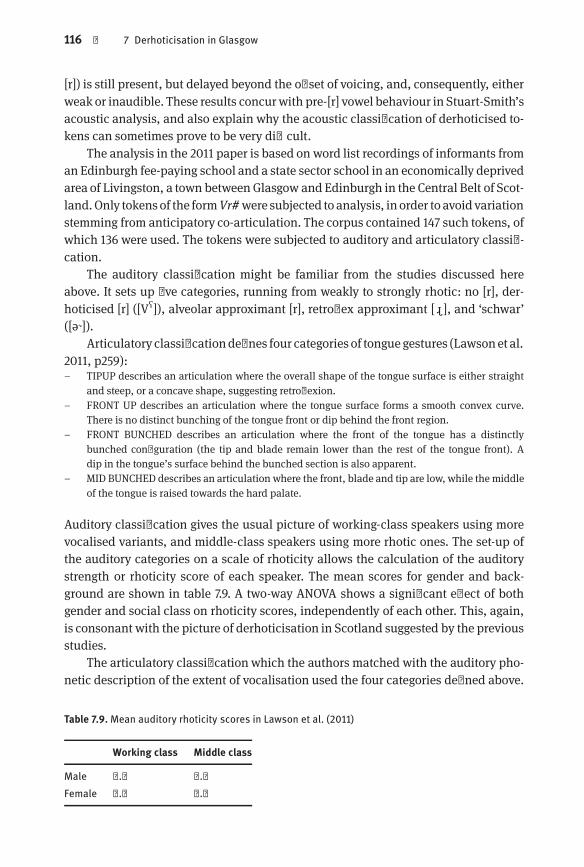
116 | 7 Derhoticisation in Glasgow
[r]) is still present, but delayed beyond the offset of voicing, and, consequently, eitherweak or inaudible. These results concurwith pre-[r] vowel behaviour in Stuart-Smith’sacoustic analysis, and also explain why the acoustic classification of derhoticised tokens can sometimes prove to be very difficult.
The analysis in the 2011 paper is based on word list recordings of informants froman Edinburgh fee-paying school and a state sector school in an economically deprivedarea of Livingston, a town between Glasgow and Edinburgh in the Central Belt of Scotland.Only tokensof the formVr# were subjected to analysis, in order to avoid variationstemming from anticipatory co-articulation. The corpus contained 147 such tokens, ofwhich 136 were used. The tokens were subjected to auditory and articulatory classification.
The auditory classification might be familiar from the studies discussed hereabove. It sets up five categories, running from weakly to strongly rhotic: no [r], derhoticised [r] ([Vʕ]), alveolar approximant [r], retroflex approximant [ ɻ ], and ‘schwar’([ə˞]).
Articulatory classificationdefines four categories of tonguegestures (Lawsonet al.2011, p259):– TIPUP describes an articulation where the overall shape of the tongue surface is either straight
and steep, or a concave shape, suggesting retroflexion.– FRONT UP describes an articulation where the tongue surface forms a smooth convex curve.
There is no distinct bunching of the tongue front or dip behind the front region.– FRONT BUNCHED describes an articulation where the front of the tongue has a distinctly
bunched configuration (the tip and blade remain lower than the rest of the tongue front). Adip in the tongue’s surface behind the bunched section is also apparent.
– MID BUNCHED describes an articulation where the front, blade and tip are low, while the middleof the tongue is raised towards the hard palate.
Auditory classification gives the usual picture of working-class speakers using morevocalised variants, and middle-class speakers using more rhotic ones. The set-up ofthe auditory categories on a scale of rhoticity allows the calculation of the auditorystrength or rhoticity score of each speaker. The mean scores for gender and background are shown in table 7.9. A two-way ANOVA shows a significant effect of bothgender and social class on rhoticity scores, independently of each other. This, again,is consonant with the picture of derhoticisation in Scotland suggested by the previousstudies.
The articulatory classification which the authors matched with the auditory phonetic description of the extent of vocalisation used the four categories defined above.
Table 7.9.Mean auditory rhoticity scores in Lawson et al. (2011)
Working class Middle class
Male 3.9 6.6Female 4.1 7.5
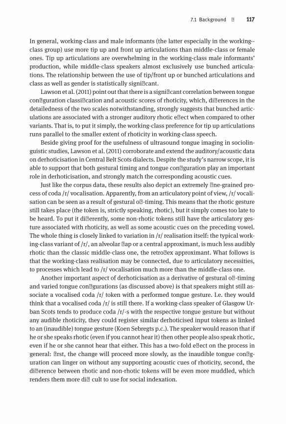
7.1 Background | 117
In general, working-class and male informants (the latter especially in the working-class group) use more tip up and front up articulations than middle-class or femaleones. Tip up articulations are overwhelming in the working-class male informants’production, while middle-class speakers almost exclusively use bunched articulations. The relationship between the use of tip/front up or bunched articulations andclass as well as gender is statistically significant.
Lawson et al. (2011) point out that there is a significant correlation between tongueconfiguration classification and acoustic scores of rhoticity, which, differences in thedetailedness of the two scales notwithstanding, strongly suggests that bunched articulations are associated with a stronger auditory rhotic effect when compared to othervariants. That is, to put it simply, the working-class preference for tip up articulationsruns parallel to the smaller extent of rhoticity in working-class speech.
Beside giving proof for the usefulness of ultrasound tongue imaging in sociolinguistic studies, Lawson et al. (2011) corroborate and extend the auditory/acoustic dataon derhoticisation in Central Belt Scots dialects. Despite the study’s narrow scope, it isable to support that both gestural timing and tongue configuration play an importantrole in derhoticisation, and strongly match the corresponding acoustic cues.
Just like the corpus data, these results also depict an extremely fine-grained process of coda /r/ vocalisation. Apparently, from an articulatory point of view, /r/ vocalisation can be seen as a result of gestural off-timing. Thismeans that the rhotic gesturestill takes place (the token is, strictly speaking, rhotic), but it simply comes too late tobe heard. To put it differently, some non-rhotic tokens still have the articulatory gesture associated with rhoticity, as well as some acoustic cues on the preceding vowel.The whole thing is closely linked to variation in /r/ realisation itself: the typical working-class variant of /r/, an alveolar flap or a central approximant, is much less audiblyrhotic than the classic middle-class one, the retroflex approximant. What follows isthat the working-class realisation may be connected, due to articulatory necessities,to processes which lead to /r/ vocalisation much more than the middle-class one.
Another important aspect of derhoticisation as a derivative of gestural off-timingand varied tongue configurations (as discussed above) is that speakers might still associate a vocalised coda /r/ token with a performed tongue gesture. I.e. they wouldthink that a vocalised coda /r/ is still there. If a working-class speaker of Glasgow Urban Scots tends to produce coda /r/-s with the respective tongue gesture but withoutany audible rhoticity, they could register similar derhoticised input tokens as linkedto an (inaudible) tongue gesture (Koen Sebregts p.c.). The speakerwould reason that ifhe or she speaks rhotic (even if you cannot hear it) then other people also speak rhotic,even if he or she cannot hear that either. This has a two-fold effect on the process ingeneral: first, the change will proceed more slowly, as the inaudible tongue configuration can linger on without any supporting acoustic cues of rhoticity, second, thedifference between rhotic and non-rhotic tokens will be even more muddled, whichrenders them more difficult to use for social indexation.

118 | 7 Derhoticisation in Glasgow
Social awareness to /r/ in Glasgow has been put to explicit test in a study by MacFarlane & Stuart-Smith (2012). The authors were generally interested in the questionwhether phonetic variation, amply shown to be sensitive to social class, age, and gender, is accessible to local listeners, as well as in the dimensions along which listenersmight classify available phonetic information. Their starting point was the ‘GlasgowUni’ accent, an emerging middle-class supra-local dialect often identified with students of the University of Glasgow and the Glasgow School of Art.
The study relied on a matched guise test (Lambert, 1967) using four phonological variables and two constructed social personae, one associated with working-classbrands, another one with middle-class ones (cf. the article for details). The three variables relevant here were (i) vowel quality before /r/ in words like ‘nerve, pearl, earth’,(ii) realisation of onset /r/ as a tap or a retroflex approximant, and (iii) syllable lengthin <-er> in disyllables, in words like ‘number, clever, cover’.
Variable (i) touches on the issue of the Square-Nurse merger, the merger of [ɛə]and [ɜː]. This is a regular feature of certain Northern English dialects, like LiverpoolEnglish, but did not happen to a large extent in Scotland (Wells, 1982). Therefore theinnovative variant would be the merged one, where words like ‘nerve’ or ‘pearl’ arerealised with [ɜː]. Clearly, the presence of the following /r/ has an influence on vowelquality, so a sensitivity to this difference hints at a general sensitivity to coda /r/. Variable (ii) directly relates to the studies discusses above: the alveolar tap is the dominantworking-class variant and the retroflex approximant is the middle-class variant bothin Lawson et al. (2011) and Stuart-Smith et al. (2007). In the data of the latter study,the 1997 corpus, /r/ realisation shows much more style shifting than /r/ vocalisation,though not as much as other characteristic variables, such as /l/ vocalisation or /t/glottalisation.
Variable (iii) is more complex. We can recall from Stuart-Smith (2007a) that thevocalic portion is longer in words with a coda /r/ irrespective of whether this /r/ isrealised or not. However, the systematic difference of vowel length between wordswith and without an orthographic coda /r/ is strongest with speakers who are mostlyrhotic in the first place. Lawson et al. (2011) get similar results, and point to gesturalre-timing as a factor in derhoticisation, which again suggests that realised coda /r/-sgo with a longer vocalic portion. However, in the MacFarlane & Stuart-Smith (2012)study, the compared variants are both rhotic, the only difference is in the length of thevocalic portion.
The stimuli consisted of word pairs recorded by the same person, a native speakerof Scottish English from Glasgow. One member of the pair was the first variant of thegiven variable, the other one the second. The listeners had to associate the heard variant to one of the two personae, one working-class and one middle-class young male(to put it simply). The experiment had 31 participants.
The results show that listeners judged the tokens belonging to one or the otherpersona, without strong preference for either. Furthermore, a significant majority ofthe tokens were judged as expected, that is, belonging to one persona or the other de
7.1 Background | 119
pending on their realisation, which supports the authors’ hypothesis on the existenceof a middle-class dialect, as defined by these variables (amongst others). If you speakin a certain way, you belong to a certain social stereotype, and the ways of speakingthat define this social stereotype are, at least partly, salient to the listener.
The results for the three variables were as follows: There was a statistically significant difference in variables (ii) and (iii), that is, attributing [ɜː] and the longer <-er>to the middle-class persona. Such a preference, however, was absent in the case ofvariable (i), as speakers did not associate taps and retroflex approximants with any ofthe personae in particular. That is, the middle-class persona would be the one whomerges Square with Nurse, and they would have a more pronounced vowel lengthdifference before a coda /r/, a property related to more rhotic accents. The tap versusapproximant distinction, however, was not associated strongly to either the working-class or the middle-class persona, contrary to expectations.
In the frame of the production data surveyed above, these results are not trivialto interpret. Sensitivity to vowel quality and quantity before /r/ strongly suggests thatthe perception of this segment is heavily linked to the previous vowel. This warns usagainst a clear segmental approach to rhoticity. Interestingly enough, whenwe look atthe 1997 corpus data, it seems that the listeners themselves failed with the segmentalapproach, inasmuch as sensitivity to coda /r/ is absent. That is to say, variation incoda /r/might only be perceived in a larger local context, that of the preceding vowel.This is further supported by the finding that listeners seem to ignore differences in/r/ realisation in the onset, where (at least in the experimental stimuli) there is nopreceding vowel.
7.1.5 Interim Summary
This chapter gave an exhaustive discussion of /r/ in Scotland. Before we go on to formulate and test a hypothesis on the speaker perception of coda /r/, it is useful to recapitulate the main points. The vocalisation of coda /r/ seems to show social stratification, and indexes speaker age, gender, and background in general. It is related tovariation in /r/ realisation, withworking-class speakers, who show a preference for analveolar tap realisation of /r/, vocalising more coda /r/-s in general. It is also relatedto vowel length and vowel quality, which correlate with the presence of orthographic/r/ and coda /r/ vocalisation: the preceding vowel is shorter in words with a writtenfinal /r/, and this length difference (and the quality difference) is more pronouncedin the use of speakers who are generally rhotic. Speakers are apparently aware of thevowel length difference according to one study in Glasgow, but do not show markedstyle shifting in coda /r/ vocalisation and are not aware of differences in variation in/r/ realisation either.
We can establish a link between these observations if we look at the source ofthe change, which is articulatory lenition, mainly the off-timing of the constriction

120 | 7 Derhoticisation in Glasgow
gesture, the main source of rhoticity. Speakers who delay this gesture sufficientlyhave no audible [r] in the coda at all, which is reinforced by the preference for tapsover retroflexes, since the former result in a weaker rhotic in the first place. Curiouslyenough, speakers can consistently produce tokens with very limited or no auditoryrhoticity but with the presence of the tongue gesture. This hints at the importanceof articulation in the spread and transmission of the change. This is even more so ifwe accept that listeners can link the non-rhotic tokens in the input to their producedtokens – which have no audible rhoticity, but a present rhotic articulatory gesture.Furthermore, the cues of [r] can spread to the preceding vowel, which complicatesmatters even more.
The situationhas twomaingrounds: thearticulatory baseof the change, aswell asthe property of /r/ to exhibit its cues less locally (i.e. more on the preceding vowel, forinstance) in the first place (Lodge, 2009; Hawkins, 2003; Simpson, 1998). This meansthat a strictly segmental approach to coda /r/ in Scottish English, or in Glasgow inparticular, is hopeless for two reasons, namely, the gradient nature of the change, andthe consequent rampant variation in /r/ realisation.
What certainly complicatesmattersmore is that derhoticisation is a loss of a property, which is obviously harder to perceive than a newproperty, such as a shift in vowelquality. Indeed, both Stuart-Smith (2007a) and Stuart-Smith et al. (2007) note thatrhotic, native speaker phoneticians found it very difficult to transcribe vocalised variants, as these are difficult to distinguish from each other and the rhotic variants. Nowonder phonetically untrained speakers do not notice them at all. And yet, derhoticisation exists in the sense that it has discernible (albeit with much difficulty) variantswhich bear a social indexing role, and therefore cannot be dismissed as a case of rampant free variation.
Such a state of affairs would no doubt lead some to question the validity of thesegment in phonological descriptions in the first place (Silverman, 2006), while others might argue that the segment is a useful heuristic tool, but not when dealing with/r/.Debates on the ontology of the segment, however, are by and large irrelevant to us,since we know that coda /r/ can be a salient marker, at least under different circumstances. In Labov’s Lower East Side study, the presence or absence of coda /r/ is thesingle most reliable marker of social status, as amply demonstrated by style shiftingin coda /r/ realisation, as well as speaker attitudes, and even overt commentary.
In the first section of this chapter I argued that the difference between Glasgowand New York City cannot be solely blamed on the first being a bottom-up, and thesecond being a top-down change, since we know of other bottom-up changes whichbecame salient for the listeners, /t/ glottalisation, extensively discussed in this book,being a prime example. The glottalisation of /t/ is a good example also in the sensethat it is also grounded in articulatory/acoustic lenition, and is salient to the listenersdespite all that.

7.2 Analysis | 121
7.2 Analysis
This section looks at data from theFredcorpus (Kortmannet al., 2005) andargues thatthe reason for the absence (or limited extent) of speaker awareness to derhoticisationis its extent of variation. This variation is certainly the artefact of the origin of thechange, but by no means should be confused with it. Glasgow (rV) evades speakerrecognition because, due to its history, it is highly variable, but that does not meanthat it cannot stabilise in the future, and hence become a social marker.
We start with the discussion of a study of coda /r/ realisation in Scotland basedon the Fred corpus. We then go on to establish transitional probabilities for coda /r/and /r/ in general, based on the corpus data. Finally, we will investigate how derhoticisation can affect these values, and, consequently, the salience of the variable.
7.2.1 The FRED study
The aim of the study was to establish the extent of derhoticisation, that is, coda /r/vocalisation, in a data set of Scottish English. The source ofmydata is the East Lothianpart of the Fred corpus (Kortmann et al., 2005). This part consists of fifteen interviewsrecorded in the late 1970s in a high school in the town of Tranent, in East Lothian inScotland, 18 km East of Edinburgh. The interviews, excluding the interviewer’s lines,consist of 33,700words. The interviewees are all then students of the high school, 15-18years old. There are fifteen interviewees, ten female and five male. Three appear in atleast three interviews, and five in two interviews. The interviewer is the same personin all interviews except for the last one. Recordings are available for ten interviews,however, two of these are of poor quality and therefore theywere not used inmy study.The remaining recordings cover 23,400 words of interviewee speech.
The target variable was word-final /r/. The reason word-medial pre-consonantal/r/-s were excluded is that both Stuart-Smith (2007a) and Stuart-Smith et al. (2007)note the difficulty in establishing whether a rhotic in this position is realised or not.This means the exclusion of 887 potential realisations in the text. Compared to the1687 word-final realisations, this is still a minority. The recordings were stereo wavfiles, sampled at 44100 Hz. Realisations were judged by the ear, using Praat (Boersma&Weenink, 2005) inmore dubious cases. I put word-final /r/-s in four categories: [R] isa rhotic realisation (a tap, an approximant, or any other possible realised variant, asin [kar] car), [V] is a vocalised realisation (where no audible rhotic is heard, as in [kaː]car), and [R/V] is an intermediate variant, e.g. with a slightly rhoticised or velarisedvowel, as in [ka˞] car. Finally, [?] is a realisation that is inaudible, either due to ambient noise or an r-initialword following it. From the 1687 tokens, 1621 were transcribed.
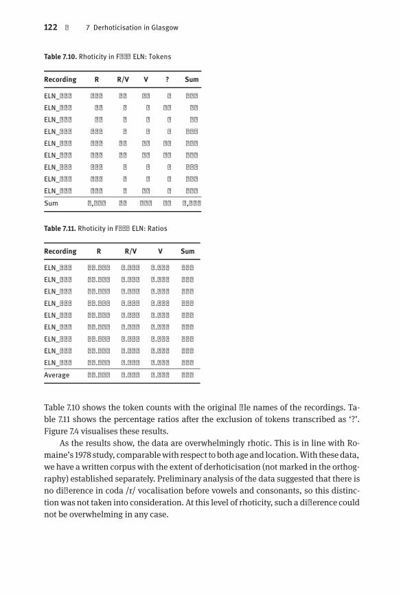
122 | 7 Derhoticisation in Glasgow
Table 7.10. Rhoticity in Fred ELN: Tokens
Recording R R/V V ? Sum
ELN_004 139 15 16 8 178ELN_005 47 5 5 11 68ELN_006 80 5 5 2 92ELN_007 103 6 7 5 121ELN_008 214 12 22 12 260ELN_009 386 14 26 10 436ELN_010 113 6 5 3 127ELN_011 123 6 5 1 135ELN_012 187 6 13 2 208Sum 1,392 75 104 54 1,625
Table 7.11. Rhoticity in Fred ELN: Ratios
Recording R R/V V Sum
ELN_004 81.765 8.824 9.412 100ELN_005 82.456 8.772 8.772 100ELN_006 88.889 5.556 5.556 100ELN_007 88.793 5.172 6.034 100ELN_008 86.290 4.839 8.871 100ELN_009 90.610 3.286 6.103 100ELN_010 91.129 4.839 4.032 100ELN_011 91.791 4.478 3.731 100ELN_012 90.777 2.913 6.311 100Average 88.056 5.409 6.536 100
Table 7.10 shows the token counts with the original file names of the recordings. Table 7.11 shows the percentage ratios after the exclusion of tokens transcribed as ‘?’.Figure 7.4 visualises these results.
As the results show, the data are overwhelmingly rhotic. This is in line with Romaine’s 1978 study, comparablewith respect tobothageand location.With thesedata,we have a written corpus with the extent of derhoticisation (not marked in the orthography) established separately. Preliminary analysis of the data suggested that there isno difference in coda /r/ vocalisation before vowels and consonants, so this distinctionwas not taken into consideration. At this level of rhoticity, such a difference couldnot be overwhelming in any case.

7.2 Analysis | 123
004
005
006
007
008
009
010
011
012
Percentages
Fred
ELN
reco
rdin
g
0 20 40 60 80 100
R
R/V
V
Fig. 7.4. Rhoticity in Fred ELN: Tokens
7.2.2 Transitional probabilities in coda /r/ realisation
The next step is to establish the transitional probabilities of a word-final /r/ in a rhoticdialect, based on these data (word-medial pre-consonantal realisations of /r/, are, dueto the difficulties they present, ignored). In order to have more robust results, I usedall the transcripts of the East Lothian interviews, even though useable recordings areonly available for eight of the fifteen in total. This procedure, however, is warranted bythe following: first, the same speakers feature in both the transcripts with andwithoutrecordings. Second, the extent of coda /r/ vocalisation is homogeneous in the recordedinterviews – a Chi Square test of independence confirms that there is no significantvariation between the recordings themselves (p=0.18). This permits the assumptionthat the extent of coda /r/ vocalisation is more or less the same within this speakercommunity, therefore the extents of vocalisation gauged from the existing interviewscan be applied to the other transcripts as well. Since the differences between stressedandunstressedpre-pausal /r/ vocalisationarenot thatpronounced in the 1997Corpus,I ignored this distinction and simply used the average – things would get complicatedlater on in any case.
Table 7.12 shows transitional probabilities based on the written part of the corpusand the derhoticisation study presented above. The first number is the probability ofa coda /r/ following a vowel: this is a general measure of derhoticisation, based onthe frequency of <Vr> final words. The second one is the probability of a word-final

124 | 7 Derhoticisation in Glasgow
Table 7.12. Coda [r] transitional probabilities in Fred East Lothian
V Cod /r/ V Ons /r/ V /r/ Cod /r/ V /r/ V Cod /r/ Ons C
Fred ELN 0.047 0.010 0.056 0.329 0.693 0.575
Table 7.13. Coda [r] transitional probabilities in Fred East Lothian and Glasgow working-class youthconversations data
V Cod /r/ V Ons /r/ V /r/ Cod /r/ V /r/ V Cod /r/ Ons C
Fred ELN 0.047 0.010 0.056 0.329 0.693 0.575Glasgow WCY 0.007 0.010 0.017 0.330 0.919 0.574
vowel followed by an [r]-initial word. This measure is based on the connected speechsequences and is independent of derhoticisation, which does not affect onset /r/ realisations. The third number follows from the previous two: it gives the general transitional probability of an [r] following a vowel, irrespective of whether there is a wordboundary in between. The fourth and fifth numbers give the probability of a coda [r]or any [r] followed by a vowel. In the former case, this is based on realised coda /r/-sfollowed by vowels, in the latter, on any realised /r/ followed by a vowel, includingonset [r]+vowel sequences. The last number is, again, a general measure of derhoticisation, as it gives the probability of a coda [r] being followed by a consonantal onset.
These numbers are, of course, not interpretable in isolation. In order to providea basis of comparison, I calculated the probabilities for the same environment basedon the same data (the written transcriptions of Fred ELN) but drawing on the resultson working-class youth behaviour in derhoticisation in the 1997 Glasgow Corpus. According to Stuart-Smith et al. (2007), young working-class speakers realise 15 per centof the rhotics in spontaneous speech, and, crucially, this is not heavily dependent onthe phonetic environment: that is, for instance, whether the coda /r/ is followed bya consonant or a vowel. This is a detail to which we will later return. If we assume,in a somewhat abstract manner, a 15 per cent general rhotic realisation, we get theset of contrasting numbers for the two dialects as seen in Table 7.13. The columns arethe same categories as above, and the lines are Fred ELN, the Fred-based data fromTable 7.12, and Glasgow WCY, the transitional probabilities based on the Fred corpusand the 1997 Glasgow study.
To recapitulate, what we see here is the difference, based on my Fred data anda study in Glasgow, between two dialects which have different extents of derhoticisation. There is, however, negligible context-dependent variation. (That is, the extentof coda /r/ vocalisation is identical before consonants and vowels.) The numbers areabstract in the sense that they do not come from actual speech patterns, but this isremedied by the fact that all sources are instances of spontaneous speech.
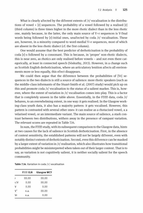
7.2 Analysis | 125
What is clearly affected by the different extents of /r/ vocalisation is the distributions of vowel + [r] sequences. The probability of a vowel followed by a realised [r](third column) is three times higher in the more rhotic dialect than in the less rhoticone, mainly because, in the latter, the only main source of V+r sequences is V-finalwords being followed by [r]-initial ones, unaffected by coda /r/ vocalisation. Theseare, however, in a minority compared to word-medial V+r sequences, most of whichare absent in the less rhotic dialect (cf. the first column).
One would assume that the best predictor of derhoticisation is the probability ofcoda [r]-s followed by a consonant. This is because, in ‘proper’ non-rhotic dialects,this is near zero, as rhotics are only realised before vowels – and not even there categorically, at least in connected speech (Sóskuthy, 2013). However, in a change suchas Scottish English derhoticisation, where an articulatory lenition affects all environments more or less equally, this effect disappears.
We could then argue that the difference between the probabilities of [Vr] sequences in the two dialects is still a source of salience: more rhotic speakers (such asthe middle-class informants of the Stuart-Smith et al. (2007) study) would pick up onthis and promote coda /r/ vocalisation to the status of a salient marker. This is, however, where the extent of variation in /r/ vocalisation comes into play. This is a factorthat is completely unseen in the table above. Essentially, in the Fred data, coda /r/behaves, to an overwhelming extent, in oneway: it gets realised. In the Glasgowworking-class youth data, it also has a majority pattern: it gets vocalised. However, thispattern is contrasted with several other ones: it can realise as a rhotacised vowel, a avelarised vowel, or an intermediate variant. The main source of salience, a stark contrast between two distributions, withers away in the presence of rampant variation.The relevant scores are repeated in Table 7.14.
In sum, theFredstudy,with its subsequent comparison to theGlasgowdata, hintsat two causes for the lack of salience in Scottish derhoticisation. First, in the absenceof context sensitivity, the established patterns will not be largely different, even withnotably distinct extents of derhoticisation. Second, even this difference canbemaskedby a larger extent of variation in /r/ realisation,which also illustrates how transitionalprobabilitiesmight bemisinterpreted when taken out of their larger context. That is tosay, as variation is not cognitively salient, it is neither socially salient for the speechcommunity.
Table 7.14. Variation in coda /r/ vocalisation
Fred ELN Glasgow WCY
r 88.05 25.04r/V 5.40 63.42V 6.53 1.86Vˆ n.a. 16.33Vr n.a. 4.43

126 | 7 Derhoticisation in Glasgow
7.3 Concluding remarks
This chapter looked at derhoticisation in Scottish English and the question of salience.I argued that derhoticisation, the vocalisation of coda /r/, an ongoing process in theCentral Belt dialects of Scots, shows very limited (if any) speaker awareness, as shownby the lack of a large extent of style shifting in data from both Glasgow (Stuart-Smithet al., 2007) and Edinburgh (Johnson, 1983), and by the apparent difficulty of middle-class Scottish transcribers to notice it. This should come as a surprise for the theoryadvocated in this work, namely, that the source of a dialectal variable’s salience is thedifference in distributions in related dialects that the variable’s behaviour entails. Ata first glance, /r/ vocalisation, which clearly relates to the distributions of /r/ realisations in the speech signal, should be a prime candidate for salience.
I went on to claim that the lack of salience in this case can be linked to thevariable’s large inherent variance – this has been shown by Timmins et al. (2004);Stuart-Smith et al. (2007). Coda /r/ can surface in many different ways, which meansthat speakers have a hard time in noticing the differences that follow from the use ofany of these variants. The reason for the variance is the source of the sound change,articulatory lenition. Articulatory and acoustic studies like Lawson et al. (2011) andStuart-Smith (2007a) strongly suggest that derhoticisation is best viewed as a gradual, phonetically fine-grained gestural reduction, which entails variation in coda /r/realisation, small differences between the individual variants, and the dispersion ofthe cues of the realised /r/, with the previous vowel playing an important role in itsidentification.
Gestural reduction as the source of the change can be linked to its bottom-up nature: it is not a norm enforced on the speaker community by the upper classes, butrather a gradient change slowly percolating through the entire community. (It has tobe stressed at this point that though real-time and apparent-time data suggests thespread of non-rhoticity, we have no solid evidence on the change sweeping throughall registers, leaving Scottish dialects without coda [r]-s.)
Based on a study on the East Lothian part of the Fred corpus (Kortmann et al.,2005), as well as the studies cited above, I investigated the transitional probabilitiestied to the different extents of derhoticisation observed in Scotland. The starting pointwas the study of derhoticisation in Fred, which, around 88 per cent, agrees with similar early studies of derhoticisation (Romaine, 1978; Macafee, 1983). I compared thislevel of rhoticity with working-class youth behaviour in the Glasgow corpus.
The first main finding was that though there is a difference in transitional probabilities, mainly in Vr sequences, that speakers can rely on, it is, in general, muchsmaller in extent, chiefly because derhoticisation, as a gradual phonetic change, iscontext-independent. Therefore, typical rhotic and non-rhotic patterns of [r] distributions before consonants and vowels are much less pronounced.
7.3 Concluding remarks | 127
The second main finding was that the extent of variation associated with largerderhoticisation effectively masks the probability difference itself. Since coda /r/ vocalisation takes place gradually, its large extent entails a large amount of variant realisations, which makes it more different to establish a comparison in distributions (forthe speakers of two dialects) and, based on the difference, use the variable as a socialmarker.
This effectively means that segmental distributions as criteria and indicators ofsalience have to be used with special care for two reasons: first, segments as abstractions have to be established especially cautiously when handling a gradient phoneticchange.
This need not mean that segments should be eschewed in general, particularlybecause a segmental approach allows the use of large corpora and leads to more robust findings. With proper heed, we can define abstract segments that give a good fiton the data. Second, it is not enough to compare the segmental distributions relatedto a particular variable in two dialects – it is also important to look at the competingvariants in a single dialect, as the more variants are possible, the less the differencein distributions for any two of them will be noticeable.
It is at this point that two comparisons are in order. Derhoticisation in Scotlandcan be readily compared to rhoticisation in New York City (Labov, 1966/2006). Thedifferences, though, are now fairly clear. The headway of coda [r] is a novel standardspreading top-down in New York City. This has two important consequences. First, /r/realisationwill bemuchmore categorical: coda /r/will not slowly come into being, butare, rather, adopted. This does notmean that language users categorically switch fromnon-rhotic to rhotic behaviour, but it reduces phonetic variation. Second, the basisfor the change is a different dialect, which compares better to the non-rhotic dialectsof the South of England than to derhoticised Scottish English, as it has linking-r, aconsistently larger extent of coda /r/ realisation before vowels thanbefore consonants.Both these effects are absent in Scots derhoticisation, and the concomitant variabilityis bothwide and large in extent enough tomask differences in segmental distributionsand hence salience in general.
This is a proper illustration of the relationship between salience and context-sensitivity, a property that follows from the model adopted in this book. If a languagechange affects segmental distributions evenly, it causes smaller transitional probability differences, and is therefore much less likely to be noticed – as shown in thischapter. Indeed, we have data (Llamas et al., 2009) that the rhoticity difference issalient between Scottish and English English dialects: speakers in towns near theScottish-English border are overtly sensitive to coda /r/ realisation,which is displayedboth in their attitudes and speech behaviour.
Crucially, lack of context-sensitivity (and the subsequent lack of salience) is notlinked to a change being top-down or bottom-up (contrary to Labov 1966/2006). True,a top-down change can proceed in such a way that different use in different contexts,and the following probability differences, will always be present. This is the New York
128 | 7 Derhoticisation in Glasgow
City example. A bottom-up change, which is often phonetically gradual, can proceedat an even pace in all environments, hence lacking pronounced probability differences. This is the Scottish example. However, a top-down change can affect a wholecategory, which might lead to absence of salience, as in the Philadelphia vowel shift(cf. Labov 1994). A bottom-up change might be sensitive to phonetic environment inthe first place, like glottalisation, where word-final pre-consonantal and pre-vocalicbehaviour split fairly early. It can also reach an equilibrium where variation turnsinto alternation triggered by the phonetic context, like Southern English non-rhoticity, where coda /r/ is realised before vowels but is absent before consonants with anear consistency.
Pertaining to the theory of salience presented in this work, a look at derhoticisation is useful in showing that a segmental approach, when handled with due care,can not only be applied to phonetically fine-grained changes, but it can also havelong-range predictions on the relationship of context-sensitivity, extent of variation,and sociolinguistic salience.
7.4 The operationalisation and relevance of salience
The previous four case studies offered practical examples to operationalising the cognitive salience of sociolinguistic variables, using a segmental approach. We saw thatthe two key features of this operationalisation were the use of corpora and attentionto context in modelling the cognitive salience of a variable.
The first three studies showed how, depending on the availability of resources, alinguist can employ the formulation of salience as put forward in this work to assesssociolinguistic variation. The fourth case study, this one, highlighted how cognitivesalience – if assumed to hinge on cognitive surprisal – is also sensitive to the extentof variation in the relevant segmental patterning.
After discussing the notion of salience as used in the sociolinguistic literature(and elsewhere) and proposing one way of defining it, the third part of this work considers the relevance of sociolinguistic salience to language theory. The following twochapters look at the consequences of differences in listener awareness, or the indicator-marker dimension, and its empirical formulations – like the present one – tomodels of linguistic competence and language change.

8 Salience and models of the lexicon
8.1 The relevance of salience
In the previous chapters, we saw examples of the link between salience and differences in segmental distributions for variables that carry social indexation and variables that do not. In this chapter, I go on to examine the role of social indexation(and, consequently, salience) in linguistic theory. Since studies onboth sociolinguisticsalience and the connection between social language use and language change generally concentrate on the phonological domain, and since all my case studies focuson phonological variables, the following two chapters remain on the sound level.
This work argues that certain sound patterns are salient. In Chapter 1 I cite evidence that humans are sensitive to differences in frequency distributions – measuredin transitional probabilities – and that this sensitivity is carriedover to sound patternsin natural language. In Chapter 3 I introduce amethod of modelling whether a certaindialectal pattern is different, ergo salient for the speaker of another dialect. The casestudies in chapters 4–7 provide examples.
A cognitively salient variable can be a potential carrier of social indexation, or,to borrow from Labovian terminology, a marker – this is contrasted with a dialectaldifference apparently neglected by the speakers, an indicator. Markers behave differently than indicators in various ways: Speakers try to manipulate them dependent onsituation and register, the most typical case being the switch to the relevant standardin a formal situation. Speakers also have implicit attitudes towards the use of markers, which can be empirically tested for, and, in extreme cases, they can point to themwhen describing a dialect.
Themarker-indicator distinction is just onewayof abstractingover listener awareness of a particular dialectal variant, which awareness is necessarily gradient in nature. Furthermore, listeners are usually alert to whole dialectal profiles (cf. the enduring geographical dialect stereotypes, such as Brummie, Scouse, Geordie, or Cockneyin England), rather than individual variation patterns (Labov, 1994). Still, the marker-indicator distinction is a useful way of thinking about research carried out on listenerawareness of sound variation and change, one that can be easily carried over to simulations of sound change as well.
So far, this work has surveyed the notion of salience in sociolinguistics. It proposed that, following the literature, we can formulate it as a property of sociolinguistic variation that affects speaker awareness to this variation. It then went on to putforward a distinction between cognitive salience, the cognitive surprisal of a variable,based on its distributions in the language use of the speech community – taking parallels with the notion of salience in visual perception as a starting point – and socialsalience, the property of a variable that triggers some extent of speaker awareness andcarries social indexation. It operationalised cognitive salience in terms of differences

130 | 8 Salience and models of the lexicon
in transitional probabilities and discussed a number of case studies which illustratea link between surprisal – cognitive salience – and social salience, the relevance ofvariation to the speech community.
Though the operationalisation advocated here has its limits, it is true thatwhethera variable is socially salient or not remains germane to linguistic theory. The third andlast part of the book considers the relevance of the distinction between socially salientandnon-salient variation for twoaspects of linguistics, themodellingof language storage and theories of sound change.
In this and the following chapter, wedistance ourselves from individual case studies and concentrate on salience and the bigger picture. The question is whether weshould assume a distinction between salient and non-salient variables outside sociolinguistics, that is, whether such a distinction leads to different predictions in anyparticular non-sociolinguisticmodel. If the answer to this first question is no, salience,irrespective of how we define it, remains a private interest of sociolinguists, centralperhaps when accounting for language attitudes, but peripheral to linguistics as awhole.
This question also leads to another one, namely, whether salience, as operationalised in this work, improves language models, whether the models gain with itin validity and descriptive adequacy.
The two questions are separate but closely linked. One can assume that salience(even loosely interpreted as the extent to which a variable carries social indexation)is relevant to linguistic theory without subscribing to the formulation put forward inthiswork. But, as I argued in Chapter 1, an empirically testable formulation of sociolinguistic salience has been hitherto missing, so a theory that wants to rely on salienceas a strict concept needs to lean on either this operationalisation or one that is similarin rigor, even if it assumes a different perspective. However we interpret salience, ourinterpretation has to be a well-defined one, otherwise we are unable to build on it anyfurther.
This chapter focusses on models of linguistic storage, or the lexicon, in order toargue that a model of the lexicon that is able to take into account the observed variation in its entirety needs to rely on the notion of cognitive salience, as put forward inChapter 1.What ismore, the types of richly detailedmemorymodels which are in needof a salience notion are precisely the ones which have such an architecture that theprinciples of this notion of salience freely follow from it. That is, a model that aspiresto envelope observed variation cannot dowithout the notion of cognitive salience, butthis notion can readily fit into a model that is indeed capable of enveloping observedvariation in the first place.
The next chapter givesmore attention to sound change and the relevance of socialindexation in the propagation of a linguistic innovation. There I will also argue that,according to available research, a testable basis of salience, however we formulate it,is necessary for an adequate description of sound change.

8.2 The duality of patterning | 131
The structure of this chapter is as follows: Section 8.2 discusses the duality ofpatterning, while Section 8.3 goes on to look at rich memory approaches to linguisticstorage. Section 8.4 provides brief conclusions.
8.2 The duality of patterning
In this chapter, I argue that the notion of cognitive salience has strong consequencesto models of linguistic competence, because it allows us to delineate salient and non-salient variation, and explainwhy the latter receives no attention from languageusers.Iwill show that amodel of language storage thatwants to account for all the structuredvariation in the speech community has to assume richly detailedmemory entries, andsuchamodelhas to rely on thenotionof salience to explaindifferent speaker reactionsto salient andnon-salient (or salient and less salient) linguistic variation.While Chapter 2 touches upon rich memory modelling, it does not go into the issues detailed inthis chapter. These issues of modelling variation will be illustrated through the problem of the duality of patterning.
The intrinsic and essential property of human language that its signs consist ofa finite set of units is called the duality of patterning (Hockett & Ascher, 1964). Phonologists, who dedicated their lives to the study of these units, approach the duality of patterning from two distinct angles. In the classic view, our observation of afinite set of phonological units presupposes the existence of an actual universal set ofphonological units, subset and phonetically implemented by different languages indifferent ways. This is the view held by, amongst others, classical generative phonology (Chomsky & Halle, 1968). A recent view has developed as a response partly todevelopments in neuro-psychology and partly to the weaknesses of the universalityargument. According to this view, the observed finite set of phonological units in anylanguage emerges from the self-organisation of a richmemory lexicon and the boundaries set by human articulation and perception (Wedel, 2007). According to this view,phonological contrast is not an inherent property of linguistic competence, rather, itemerges from the general properties of a richly detailed lexicon.
Certain sociolinguists, especially sociophoneticians, have met the notion of arichly detailed lexical storage with enthusiasm. Sociophonetics, a relatively newoffshoot of variationist sociolinguistics, is occupied with the description of smallphonetic differences, which correlate with context and social background (Foulkes& Docherty, 2006). The existence of socially bounded phonetic variation stronglyimplies that a lot more detail is available to the speaker than what has been assumedby the universalist school. Differences that have been previously regarded as a part oflow level phonetic implementation are able to index social background or region oforigin. This makes it necessary to suppose amore detailed linguistic competence, one

132 | 8 Salience and models of the lexicon
that is able to keep track of phonetic detail, which has previously been thought to beaccidental and, from the sociolinguist’s point of view, largely irrelevant.
Richmemory sociophoneticmodelling is confrontedwith a serious issue, one thatis inherited from general linguistics with the framework itself. If all phonetic detail isavailable to the speaker, if a large extent of phonetic variation is used to mark socialvariation (like the social background, age, or gender of the speaker), we expect listeners to react to all of it. As this work has already demonstrated in detail, speakerawareness to linguistic variation is uneven – certain variables are more salient thanothers.
This chapter argues that the notion of sociolinguistic salience, based on cognitive surprisal, is able to account for this issue. This formulation, of course, greatlyrelies on a rich memory lexicon and the notion of language use actively affecting language structure. Indeed, a richly detailed storage is a prerequisite for the concept towork. From a modelling point of view, the original problem of invisible versus salientvariation also follows from the assumption of a rich storage. Therefore, the cognitivesalience concept can provide an answer for this problem remainingwithin the boundsof the rich storage model, not making the model stronger in the process.
8.3 Modelling, phonetic variation and indexationModels of the phonological storage describe the way word forms are stored in the individual language user’s memory. These lexical entries are then accessed by a phonological architecture for purposes of production (in which case a lexical entry is implemented and sent off to articulation) or perception (in which case auditory input ismatched on the entry). The assumed shape of the lexical storage shares an intimateconnectionwith the shape of the phonological architecture relying on it – for instance,if the lexical entry of aword is free of redundantphonetic information, a separatemodule has to supply this information before theword is articulated. Or, if onlyword formsare stored, a separate module is responsible for concatenating these words forms intoan utterance, e.g. a whole sentence. If the word form is stored with phonetic detail,and/or if a longer utterance is stored in itself, the workload of the phonological architecture is smaller. This is, however, beyond the scope of our discussion.
Structuralist assumptions of word storage greatly rely on the classic, Aristotelianview on classification. In this view, entities have essential features, and these featuresestablish the basis of assigning category membership to them. They also have accidental features, but these do not add to their classification, rather, they follow fromthe category membership itself. This can be easily applied to phonology as well: ataxonomic phonological classification regards the contrastive sound segments of thelanguage, the phonemes, as the essential features of a word form, while everything

8.3 Modelling, phonetic variation and indexation | 133
else (phonetic variation in the form’s realisation, the form’s frequency, its typical context, and so on) is accidental.
Classical generative phonology, the successor of taxonomic phonemics as themain theory of phonology in the 20th century, does not stray from the minimal memory assumption inasmuch as it proposes an underlying representation, consisting of apre-supposed alphabet of distinctive features with feature specifications (Chomsky &Halle, 1968). What is relevant to us is that, in this view, we start out with stripped-offlexical representations, and phonetic detail is added only during the course of articulation. Consequently, no information is stored beyond the minimal, contrastivesegments. The minimal memory model does not reckon with word frequency, collocates, or phonetic variation.
Early variationist sociolinguistics builds on theminimalmemorymodel – and, indeed, the whole phonological architecture – of classical generative phonology (Cedergren&Sankoff, 1974). Observedphonetic variation ismodelledusinga rule-basedgenerative architecture – it is interpreted as the result of probabilistic rule application on afixed underlying representation. This approach can be seen as an attempt to compressphonetic variation into the structure of classical generative phonology. While the notion of variable rules is problematic in itself (Coleman, 2005), it alsomakes it impossible to find deterministic links between observed phonetic variation and extra-linguistic effects (extra-linguistic in the generative sense), like frequency, context, or style.This is because output (i.e. phonetic variation) remains probabilistic. True, we can assume that a speakerwith a different social backgroundhas ‘learned’ or adjusted different probabilities to his or her variable rules, but that still excludes context-dependentstyle-shifting or listener awareness to phonetic variation, since these are still probabilistic. (It is possible to shovel these into a variable-rulemodel aswell, but this modelwill be very hard to distinguish from one that assumes rich memory representations.)
A radically different conception of phonological storage emerged in the 1990s,partly as a response to the groundbreaking research of Eleanor Rosch and her successors on categorisation (Rosch, 1973; Lakoff, 1987). This research shows that people aresensitive to accidental properties during categorisation tasks. That is, the redundantdetails of an object or the frequency withwhich it is encountered has a strong effect onthe category label the object attains, and on category labels in general. In phonetics,this notion is implemented by Johnson (2005b). He argues that, during speech perception, we do not strip away redundant information to match an encountered formwith an entry in our lexicon (the process of speaker normalisation). Rather, we storea vast number of encountered tokens along with rich phonetic detail, and comparea new form to all pre-existent exemplars in our memory in order to identify it. Thestored exemplars are also tagged for the speaker (that is, the person who said them)and the context in which they occurred. According to Johnson, this approach is ableto account for both word and speaker recognition.
Rich memory models of phonological storage are championed, amongst others,by Wedel (2007), who shows how phonological consistency (such as the existence of

134 | 8 Salience and models of the lexicon
a finite set of contrastive segments, the cornerstone of the duality of patterning) canemerge from a richly detailed lexicon of encountered word tokens or exemplars.
In Chapter 1, we already discussed rich memory modelling in detail. Indeed, thecase studies are also examples of structured variation that requires richmemorymodelling. Sociophonetic literature marshals a large amount of further evidence on thecorrelation of phonetic variation with age, gender, social background, and context.Fabricius (2000) shows the sensitivity of upper-class speakers to glottalisation inSouthern English. Milroy et al. (1994b) go one step further and provide evidence onhow two separate glottalisation processes are present in the Tynemouth area in andaround Newcastle, and how listener sensitivity differs for these two processes. Thenewer, ‘imported’ pattern of word-medial glottalisation is noticed by the listeners toa much larger extent than the older, local process of pre-glottalisation. MacFarlane &Stuart-Smith (2012) illustrate how fine phonetic variation is associated with differentspeaker personae in Glasgow, and Campbell-Kibler (2011) has similar results from alarge-scale study on American English. Stuart-Smith (2007b) notes how small differences in the articulation of /s/ are socially stratified in Glasgow, while Lawson et al.(2011) has similar results on /r/ in Edinburgh and other parts of Southern Scotland.As Labov (2001) remarks, similar small differences in vowel articulations can be alsosocially stratified and subject to listener awareness. Hay et al. (2006) finds evidenceon preconceptions on speaker identity affecting the boundaries of phonetic categoriesin speech perception in New Zealand English, and Jannedy et al. (2011) have the samefinding in Berlin German. Hall-Lew et al. (2010) show how small-scale adjustmentsin phonetic realisation can be related to style and context in American English. Otherexamples are not hard to find.
To recapitulate, socially stratified and context-dependent phonetic variation cannot bemerely probabilistic. In order tomodel variation of this kind, one has to assumea richly detailed lexical storage. (Whether this storage is also used for phonologicalprocessing is a wholly different matter, though one could argue that, if we have to assume it anyway, it might as well serve this purpose as well.)
If people can have preconceptions on the phonetic characteristics of [s] depending on the part of the town the speaker comes from (Jannedy et al., 2011), we rightlyexpect them to show a great deal of sensitivity to all kinds of socially stratified variation. However, as shown in depth in this work, is not the case. The indicator/markerdimension (or the notion of sociolinguistic salience) is problematic for rich memorymodelling: if language users are able to store and re-produce socially stratified phonetic variation, we have to explain why they are only sensitive to a subset of it.
This is where the notion of salience – as advocated in this work – comes into play.As seen in Chapter 6, we can look at two patterns of phonetic variation and modeltheir cognitive salience in order to predict whether they will carry social indexation.We can then argue that while both variation patterns are stored in the individual’slinguistic storage (which is proven by their recurrence in production) only one of the

8.4 Summary | 135
patterns is surprising or distinct enough to be cognitively salient and, in turn, carrysocial indexation.
The beauty of the analysis is that it relies on richmemory storage in order to solveone of the major problems associated with rich memory storage in sociolinguistics.As we can recall from earlier in this chapter, this problem is that rich memory modelsover-generate. They lead us to expect all types of variation to be available to socialindexation, whereas this is clearly not the case. This analysis amends the rich memory model relying on the intuitive notion that only a subset of the totality of variationis stored, and, in turn, only a subset of the stored variation is salient enough to benoticed, even in an unconscious manner.
Cognitive (and social) salience and rich memory-modelling elegantly rely on eachother. We can only interpret cognitive salience as a consequence of differences in segmental distributions caused by the variable realisation of a linguistic variable if we assume that language users are able to keep track of these differences, and this requiresus to work with a rich memory model. Rich memory models do not trivially accountfor the observed difference in socially salient and non-salient linguistic variation, butthis can be rectified if we recur to the concept of cognitive salience.
8.4 SummaryIn this chapter, I argued that salience has consequences for theory building beyondsociolinguistics. The first example was the modelling of linguistic storage. I showedthat models which are able to take into account all observed structured variation arein need of an explanation as to why some types of this variation are invisible to thelanguage user. I went on to claim that one way of separating salient and non-salientvariation is the theory of salience as discussed in this book, especially since its principles readily follow from rich memory model architecture.

9 Salience and language changeThe previous chapter has shown that sociolinguistic salience explains the observeddiscrepancy between the production and perception of structured variation in richmemorymodels of linguistic storage. This chapter looks at the role of salience in soundchange. Unlike in the case of the previous chapter, one does not have to vouch for thetheory of salience put forward in this work in order to accept the conclusions of thischapter, that salience is relevant to sound change. However, as we will see, there arecaseswhere differences in distributions do seem to coincidewith patterns of variationassociated with salient versus non-salient sound changes. Evidence for the parallelbetween cognitive salience and sociolinguistic salience in the diachronic domain isanother argument for the theory presented in this work. The focus of the chapter islanguage change of the phonological kind.
The chapter consists of two main sections and a summary. In Section 9.1, I review the role of speaker indexation in sound change, surveying theoretical work andquantitative studies. We will see that the literature is more and more accommodatingto the relevance of social dynamics in sound change, from the clear-cut rejection ofthe Neogrammarians to gaining ground in contemporary models of language change,heavily influenced by social anthropology.
Thismain section focussesbothon the sociolinguisticworkon speaker indexation(Section 9.1.1) and the empirical studies and simulations for evidence on the connection between group indexation and sound change (Section 9.1.2). We will see that theavailable body of facts suggests a view of sound change where the language user’s attempt at indexing identity and interactions between individuals both play a relevantrole in shaping the course of sound change. The section concludes with the discussion of two computer simulations, both hinting at the importance of social indexationin the propagation of sound change. I will discuss a modelling set-up in which anexplicit distinction is made between variation with and without social indexing. Particular attention is given to the model of language change by Baxter et al. (2009), animplementation of the evolutionary theory of Croft (2000).
Section 9.2 connects Baxter et al.’s (2009) model to two further case studies inorder to further illustrate how variants that carry social indexation, and thereby varyin salience, behave differently from variants that do not do so in the course of soundchange. This section integrates the chapter into the structure of the book by showinghow these examples can be approached using the notion of cognitive salience, basedon differences in segmental distributions. Section 9.3 gives a summary.
As noted in Chapter 1, social indexing is interpreted rather generally as social information attached to structured variation in the language community. This readingsuffices to underline the main point of the chapter, namely, that social informationcounts – the preferences of the language community influence the propagation of socially salient variants and sound change is better understood if we assume that socialsalience can play a role in it.

138 | 9 Salience and language change
9.1 Speaker indexation in sound change
The fact that salient variableswhich carry social indexation (that is,markers) are useddifferently by speakers does not directly imply that these behave differently in soundchange. This latter assumption has two premises, (i) that salient variables do carrysocial indexation, and (ii) that social indexation shapes sound change.
I will brief on the first premise: On the one hand, cognitively salient, socially stratified variables are likely to become social markers. On the other hand, social markers,wherever the probability-based theory of salience is applicable to them (see the Scottish example in Chapter 7), should always have cognitive salience, i.e. entail a lowtransitional probability in the speech signal.
The second premise, that social indexation is connected to sound change – not tomention guides it – is less obvious.
9.1.1 Approaches to speaker indexation
The Neogrammarians see sound change as an unstoppable force working above thespeakers’ heads (Paul, 1886/1995), wholly resistant to influence by any language userand independent of language use as awhole. This tradition is upheld by the AmericanStructuralists (Sapir, 1921; Bloomfield, 1933), who regard sound change crucially notonly as untouchable but also as invisible to the speaker.
The Structuralist reluctance to acknowledge the speaker in anywaypartly followsfrom Saussure’s 1916/1995 Langue–Parole distinction, which draws a line between thelinguistic structure, which can be altered ‘globally’ by language change, and the people who actually use it to communicate. Disenfranchising language use is also partlya reaction to unfortunate earlier claims on the direct effect of the climate and socialdevelopment on linguistic structure (cf. comments in Trubetzkoy 1999).
Weinreich et al. (1968) and the variationist sociolinguist school established intheir wake, including works like Labov (1972b), challenge the notion of sound changeas a law of nature. This, in turn, allows them to consider the speaker as an actor andsocial indexation as a potential factor in sound change. They are, however, cautiouswith the subject – in their opinion, the social values associated with variables have anapparent influence on the course of the change, but mainly in a robust and deterministic manner. Sound change, when vulnerable to speaker influence, is steered by theprestige of certain speaker groups and the larger community’s adherence to the localnorm.
The classic variationist sociolinguistic tradition, to which this work owes much,associates particular linguistic variants with membership in broadly defined speakergroups, usually beingpart of a clear social hierarchy. The preference of a variant, then,can signal affiliation to speaker groups of various types. Examples include a rooted,
9.1 Speaker indexation in sound change | 139
geographically outlined speaker community, as in the case of the centralisation of thediphthongs [aɪ] and [aʊ] in Martha’s Vinyard (Labov, 1972b), a wide social class, as inthe case of the use of a stop variant for the standard dental fricative in New York City(Labov, 1972a), an age or a gender group, or most likely a combination of these, as inthe use of the high rising terminal intonation pattern with young female speakers inNew Zealand (Britain, 1992), or the youngmale working class speakers’ preference forthe vocalised variant of /r/ in Glasgow (Stuart-Smith, 2003).
The language use of certain social groups, typically those with a better socialstanding, has overt prestige – it is often regarded as the standard of the language variety, which results in the overt or covert stigmatisation and avoidance of the non-standard variants – as discussed at length in the present work. Non-standard, vernacularvariants, however, are attributed covert prestige (Trudgill, 1974), whichwould explainwhy they persist in spite of the pressure of the standard. One way to evaluate variantsis to interpret their social indexation as the amount of prestige they enjoy, with somevariants being less prestigious than others, which is to be mirrored by the languageuse of larger social groups, like lower middle-class speakers or educated women.
Themain contributions of variationist sociolinguistics is the nowwell-establishedfact that sound change is observable in progress, along with the valuable insights toits mediation (or propagation) in the speech community, guided by prestige. Althoughthere is a tacit understanding that overt prestige is associated with correctness, education, and high social standing, whereas covert prestige with solidarity, friendliness,and neighbourhood identity, Labov (2001) duly notes that evidence on the existenceof covert prestige is controversial. He quotes attitude studies from Philadelphia thatshow that variants allegedly enjoying covert prestige never have the upper hand inattitude tests, irrespective of what aspects subjects are given to score them. That is, inthese studies, a speaker voice using a vernacular variant with alleged covert prestigewould score low not only on educated but also on friendly or empathetic.
In comparison, the existence of overt prestige is copiously supported by empiricalevidence, including self-reports, popular stereotypes, and attitude tests (cf. e.g. Labov1966/2006). Indeed, as Labov notes, the only solid evidence for covert prestige is thestubborn refusal of urban vernacular dialects to die out (cf.Williams & Kerswill 1999).
In the classic variationist view, the speaker is notmuchmore than a vessel of sociolinguistic factors, and the personal influence over the choice of identity is, to a largeextent, underplayed. (Cf. the notion of the cultural dupeGiddens 1979.) Social practicein this case comes down largely to adherence to the norm.
Social structure and the role of the speaker are connected in classic variationist sociolinguistic research,which typically concentrates on urban centres (such as Trudgill(1974) on Norwich or Labov (1966/2006) on New York City). One way to put it is thatsociety is a big ladder that speakers try to climb. The use of the terms overt and covertprestige mirrors this, as does the typology of sound change proposed in these works.Change from above is a conscious change that is introduced by the leading group,whohold onto the overt prestige form. Change from below enters under cover, originating
140 | 9 Salience and language change
in a lower, non-prestigious social group. Change from above is, then, robustly categorical in structure, while change from below is gradient and phonetically fine-grained.This issue has been discussed in detail in Chapter 7.
Potential inherent weaknesses of the variationist tradition are highlighted by theworks like Milroy (1980) and Eckert (2000). These both develop on the classic modelbased on the primacy of social class-based speaker categorisation and put a largeremphasis on speaker organisation into social networks. According to both Milroy andEckert, language use is better seen as guided by identity formation in the field of communities of practice, social grouplets organised around a particular shared activity,hobby, profession, or habit, and not solely driven along the lines of broadly definedsocietal units specified by economical status, age, or gender. This is true even moreso since some of these categories, like economical status or, especially, gender, aredifficult to define in broad terms.
To take the example of gender, on the one hand, binary categorisation of gendermembership (female/male) is oversimplified and potentially masks finer patterns ofvariation present which depend on, for instance, the extent to which an individualassigns herself or himself to a gender group. On the other hand, even though genderis always investigated as a subordinate factor to social class, in cases it can account formore variation in sound change alone than in conjunction with class (cf. e.g. Cheshire2002).
A network-based approach is also supported by the fact that, contrary to whatthe classic variationist model of urban language use would lead us to believe, manycompeting norms can emerge in a community. This is apparent, for instance, in thestudy of Stuart-Smith et al. (2007) on language use in Glasgow. In this study we findcases where the vernacular variants are played up in formal interview settings, andthis can be seen as an open emphasis on the norm, but, in this case, the vernacularnorm.
Network-based studies take it for granted that the formation and maintaining ofidentity plays a role in the linguistic behaviour of any particular social network. Thisinvolves adherence to or rejection of a norm variable and the use of innovative vernacular variants to define the group with respect to other groups, and to express groupsolidarity.
In sum, speaker indexation is gaining significance in quantitative studies on thesocial context of sound change. The interaction between speaker indexation andchange is also apparent in simulations used to lay out and investigate the mechanicsof language variation and change.
9.1.2 Simulations on the role of indexation
This section details two simulations of language change. The reason I talk aboutthem at length is that the first one, by Roberts (2010), gives an elegant account of the

9.1 Speaker indexation in sound change | 141
emergence of markers in language use, while the second one, by Baxter et al. (2009),presents a framework in which the effect of speaker indexation – and, indirectly,salience – on sound change can be assessed directly.
Roberts (2008, 2010) sets out with an evolutionary approach to language change.He argues that, from an evolutionary point of view, co-operation – a typical humantrait – is beneficial, since groups are better at utilising available resources than separate individuals. Group behaviour, however, brings forward the free-rider problem:individuals could potentially travel from group to group, exploiting the groups’ altruistic, co-operative behaviour, and exploiting each, only to move to the next groupwhen the previous one recognised their selfish behaviour and excluded them.
The best way to battle free riders is to create group markers which identify groupmembers, and therefore also outsiders. This relates to the original assumption on themulti-facetedness of communicative utterances: an utterance can signal that an individual demands certain resources, but it also signals the individual’s membershipin the group, with the potential consequence that, as a group member, the individual is obliged to return the favour later. Roberts notes that language is one of the bestidentity markers: it is robust, reliable, takes a long time to develop, and is, therefore,resistant to changes.
Hismain research question iswhether linguistic groupmarkers developnaturally,during the course of group interactions, or whether identitymarking also has an effecton them. This is precisely the question, albeit formulated differently, that I talk aboutabove. In order to answer it, he develops an experimental paradigm of group interactions, based on an artificial language and a competitive situation in which resourceshave to be shared.
During the experiment, participants have to learn an artificial language first. Thisis required because what he is interested in is whether they would develop groupmarkers, so he has to exclude the participants’ native language, already rich in complex patterns of social indexation. After this first step, the experiment consists of anumber of rounds. Each round starts with interaction: participants command a poolof resources, and they are paired with another participant to discuss trading these resources. Giving someone resources multiplies their value, so participants are betteroff when they trade with each other rather than sit on resources and not share withanyone else. The discussion phase is followed by actual tradingwith the previous discussion partner, where participants can decide whether they oblige to their requestsor ignore them. Finally, participants get a summary of trade in that round.
The experiment has two independent variables. The first one is competitive versusco-operative: In the competitive condition, players are divided into two teams. Teamscores are calculated at the end of each round, and the teamwith a highest final scorewins. In the co-operative condition, all participants belong to the same team, and thesole aim is the accumulation of resources (for details, see Roberts 2010). The competitive condition, in which participants cannot tell if they are talking to a team memberor an ‘enemy’ in the discussion phrase, encourages the use of the artificial language
142 | 9 Salience and language change
to signal teammembership beside its basic purpose of communication. This pressureis absent in the co-operative condition. In the competitive condition, participants areasked after each round whether they were able to recognise their team mates.
The second independent variable is frequency: in the low-frequency condition,the participants have 15 rounds, in the high-frequency one, they have 30 rounds.
Roberts has two predictions for the competitive condition, (i) that players wouldbe able to identify their team-mates using only linguistic cues, and (ii) that the alienlanguage, identical for all players at the beginning of the game, would diverge intodialects.
The main results confirm these predictions, but only in the high frequency condition. In this condition, players do significantly better than chance at recognising theirteam mates when asked after each round, and this also shows in their habits of resource exchange. Dialect divergence, that is, the increase in the number of variantsused for each word, is clearly observable in the high frequency condition.
Roberts goes into detail about this dialect divergence, and the various communicative strategies used by the participants to recognise their team mates. What isrelevant to us is that, in his experimental setting, competitive behaviour results inthe rapid development of linguistic markers. This strongly suggests that individualrecognition/individual self-assertion plays a relevant role in the emergence of linguistic markers, and, consequently, in language change in general.
If we interpret social indexation as encompassing general labels such as groupmembership, Roberts’ findings will underline the importance of social salience in language change, supporting the view of sound change proposed in network-based sociolinguistic studies, such as Milroy (1980). Socially salient variants are precisely theones which are used to indicate group membership, and the paradigm discussed byRoberts clearly points at their relevance in social language use.
His findings also provide evidence on how speakers utilise variation that arisesfrom independent circumstances (such as the noise in transmission and learner errors) to create group identity markers, a process acknowledged by, amongst others,Foulkes & Docherty (2006). Speaker indexation and sound change are then inseparable. There is, however, another important question that Roberts does not address,namely, the way variants that carry social indexation behave differently from thosethat do not – the consequences of the marker/indicator distinction on sound change.
This is a core problem in the simulation discussed in Baxter et al. (2009), whichaims at modelling the emergence of New Zealand English. Before we are able to seehow their model works, we have to briefly look into both their theoretical foundationsand the particular example they set out to model.
The network-based model of language change that their simulation takes as apremise is proposed byCroft (2000). Croft takes parallels betweenbiological evolutionand language change as his starting point, positing interactions between individualsas the source of both the actuation (emergence) and propagation (spreading) of novelvariants.
9.1 Speaker indexation in sound change | 143
Starting on an evolutionary premise adopted partly fromDawkins (1976) and Hull(1988), Croft establishes two principal units of change. The replicator is a piece ofstructure replicating itself, while the interactor is the entity that interacts with its environment in such a way as to cause replication to be differential. In biological evolution, the replicator is the gene, and the interactor is the organism, which has a certainchance to produce offspring, partly affected by its adaptation to the environment, andpartly affected by pure chance.
In language, Croft argues, the replicator is the utterance, a multi-structured linguistic unit used to express a certain type of convention. The interactor is the speaker,and replicators, that is, utterances, are replicated during face-to-face interactions: onespeaker, based on his or her linguistic competence, formulates an utterance, which isthenprocessedand storedby the listener. Crucially, this is indirect replication, affectedby noise (in a very concrete sense, here) and the listener’s linguistic competence. Thisextensively reduces the chance of successful identical replication, explainingwhy language change proceeds much faster than biological evolution. (Another obvious reason is that utterances are replicated – in Croft’s sense – much quicker than genes.)
There are obvious differences between the behaviour of a gene and anorganismasreplicator and interactor vis-à-visutterance (or set of structure) and speaker. Assumingan exemplar-based cognitive framework, relying on spreading activation (e.g. Rumelhart &McClelland 1987), it is reasonable to take the imperfect replication of utterancesas the source of linguistic innovation – and actuation. The propagation of a linguistic variant is a different issue, because, though innovation, in its strict sense, is omnipresent (no utterance is repeated twice verbatim), this does not lead to uncheckedvariation in the language.
Croft talks indetail about theactuation, theorigin, of a new linguistic variant. Thiswork, however, largely ignores the actuation problem. This is true for this chapter aswell. It is intuitive to think that salience comes into play when a variant is transmitted, since this is precisely the point in time when the listener can notice or ignore it.Therefore, below, I concentrate on propagation in Croft’s model.
In thismodel, twomain factors affect propagation: On the onehand, the frequencyof an actuation will have an effect on the success and speed of its propagation. Thefrequency of listener exposure to a particular innovative variant depends on both itsprobability to emergeduring innovation, and the listener’s position in the speech community – the listener might be a member of a social network that uses this variantprevalently. Only taking frequency into account, the success of a new variant ismostlydue to chance. The same innovation can spread quickly if proposed in a well-connected speaker group and fade if proposed in a small one. Certain types of changes occurwith a higher chance and aremore likely to be transmitted successfully than others(cf. Keller 1994). This factor, however, is below thedetail of themodel discussedabove.
On the other hand, innovative variants might have social value attached to them,and this promotes (or hinders) their transfer by listeners. Simply put, an innovationcan propagate faster if it is frequent in the first place, and if it sounds cool.
144 | 9 Salience and language change
Baxter and colleagues build on this premise and note that the spread of a novelvariant canbemodelled in twoways. Since language is used ina community, a speakerismore likely to interactwith certain speakers thanothers, dependingon the speaker’ssocial network. This, in turn, candepend on geographical and social factors.What follows is that even if we do not order utterances based on social value, the frequency ofinteractions can give an advantage to certain utterances over others. This is what theycall neutral interactor selection. This stands in comparison with weighted interactorselection, where utterances can be preferred or avoided based on their social value. Inthe case of neutral interactor selection the only effect on the propagation of a variant isits frequency, in the case of weighted interactor selection, both frequency and prestige(social value) play a role. (Note that frequency here is a complex concept: if variantsA and B have the same token frequency in the beginning, variant A can spread whilevariant B can die out if, for example, variant A originates in the largest and best connected speaker group, while variant B is present in more, peripheral, smaller speakergroups simultaneously. For details on the mechanics of the model, cf. Baxter et al.2006, 2009.)
The reason they propose this distinction is that they want to test a claimmade byPeter Trudgill (cf. e.g. Trudgill 2008), that the emergence of New Zealand English, likeall other colonial English dialects, is purely deterministic, without any influence ofwhat people at the time of dialect formation regarded as preferable or prestige forms.Though Trudgill mostly uses prestige in the sense of the prestige carried by the Standard English variants of the time, his argument is clearly all-encompassing: simplyput, the emergence of a colonial English dialect, such as New Zealand English, is onlyattributable to the background, number and geographical distribution of its speakers – from a sociolinguistic point of view, purely to chance.
Baxter et al. (2009) take on this claim and model the emergence of New ZealandEnglish using Croft’s terminology. Translated to this terminology, Trudgill’s predictionwould be that this dialect emerged through neutral interactor selection only. They findthat neutral interactor selection alone is insufficient for the dialect to reach its presentstate in the allotted time frame.What follows is that, at least to some extent, weightedinteractor selection also has to play a role in its emergence.
To be precise, the actual results of this model – for a fairly specific situation, dialect emergence in isolation– ismuch less relevant toushere than themechanicsusedfor the simulation. Baxter and colleagues model the spread of indicator and markervariables in a speaker network, and this is an ideal basic set-up for a model of the roleof salience in sound change.
Themain consequence of their model is that variants that propagate via weightedinteractor selection, that is, markers, spread differently from indicators, variants thatspread through neutral interactor selection. The main difference is that, given propertailwind, the former spreadmuchquicker. In thismodel, the effect of prestige on propagation is taken for granted.
9.2 Salience in the propagation of a change | 145
The theory of salience presented in this work is able to input a network-basedmodel of sound change on which variants are salient, can possibly carry some formof prestige, and as a result spread differently. One prediction is that a prestige variantis adopted more readily by a larger number of speakers, spreading quickly out of thegroup inwhich it is actuated and reachingnewnetworks. Aneutral variant propagatesat a slower rate, and is more likely to remain in the group where it is actuated.
Salience, then, is crucial to our understanding of the propagation of a soundchange.
That there is such a difference between salient marker and non-salient indicatorbehaviour in real life can be seen in the two case studies presented here.
9.2 Salience in the propagation of a change
Milroy (2007) proposes a distinction between two typical ways of the propagation ofa sociolinguistic variant. Off the shelf changes are readily accessible to a large number of speakers, while under the counter changes spread in a socially and geographically more limited domain. Conflating her distinction with levels of social awarenessthrough the Croft model of language evolution is a tempting one. One could arguethat the propagation of markers is propelled (or hindered) by weighted interactor selection, so if it is propelled, it is more easily available to a larger number of speakersin a shorter time span. At the same time, an indicator is restricted to a smaller domainas its propagation is only propelled by frequency.
The concepts socially salient variant,marker, off-the-shelf variant andweighted interactor all describe the same thing, the distinction between types of structured variation that are invisible for language users and that are subject to social awareness. Inthis book, this distinction is one of social salience and I argue that, at least in certaincases, it has to be underlined by cognitive salience.
We expect that socially salient variation shows different patterns of use to non-salient variation. Languageusers attribute socialmeaning to it andadopt and transmitit more readily. (Or, indeed, that they reject it more readily.) This is the picture thatemerges if we compare glottalisation in the South of England with derhoticisation inScotland, two variation patterns discussed in detail in Chapters 5 and 7, respectively.
9.2.1 Glottalisation in England
Certain patterns of glottalisation, the replacement of a voiceless coronal stop witha glottal stop, show similarities with what Baxter and colleagues call propagationthrough weighted interactor selection. Glottalisation has been discussed in Chapter 5in detail. To recapitulate the main findings, Glottalisation is originally a Southern En

146 | 9 Salience and language change
glish English feature, typical of the working-class speech of London, that is rapidlyspreading in use, reaching bothmore formal registers and other cities in England, beingmostly associatedwith urban speech (see also Roach 1973;Wells 1982; Kortmann&Schneider 2004). (The birthplace of glottalisation in the British Isles is likely Scotland(Andrésen, 1968), but that is irrelevant here.)
It is interesting to note that the spread of glottalisation in London resembles achange from below in the sense that it originates in lower-class speech and that it isboth phonetically gradient (with realisations ranging from pre-glottalised variants toglottal stop variants) and, in itsmore prevalent forms, ignored by the speaker community. It is only word-final pre-vocalic glottal replacement (the focus of Chapter 5) andword-medial intervocalic glottal replacement that are salient for speakers. We havegood evidence that precisely these two patterns are the ones that behave differently inother UK cities – as far as glottalisation patterns go, these are the interesting ones.
Milroy et al. (1994a), in a paper on glottalisation in Newcastle upon Tyne, surveythe rapidity with which glottal replacement increased in in cities throughout the UK,such as Cardiff, Liverpool, or Belfast. They note that in Newcastle the glottal replacement pattern actually competes with a local pattern of glottal reinforcement, a kind ofphonetic variation that is similar but not entirely identical to it. Glottal reinforcement,the co-articulation of a glottal constriction with the oral constriction in the case of thelenis stops [p],[t],[k], is a local, entrenched variety, which also shows a large extent ofphonetic variation with a uni-modal distribution. It is a local prestige form usedmorepredominantly by men. Glottal replacement, the replacement of the oral constrictionwith a glottal one in the case of the lenis stop [t], is the new variety, which has a bi-modal distribution: to a large extent, coronal stops are either replaced by glottal stopsor not. It is more restricted than glottal reinforcement, only showing variationwith [t].It is more typically used by women.
Milroy and colleagues argue that, while the two showphonetic similarities, glottalreinforcement and glottal replacement are two distinct patterns of variation in Newcastle and the Tyneside. The latter is a supra-local norm that was imported to thisurban centre, supported by the fact the kind of gender bias shown by its use: womenfavour it more than men. In variationist studies of urban speech, women opt for thestandard variant,whichmakes it surprising that they would take the lead in the use ofglottalisation, an iconic English English sub-standard pattern. Milroy and colleaguesreach the conclusion that this apparent contradiction is explained if we see this pattern, glottal replacement, aspart of anemergingmiddle-classnorm in theBritish Isles,a norm to which female speakers in Newcastle converge.
The reader might observe that the supra-local glottalisation pattern, glottal replacement, behaves in a way that Baxter et al. (2009) would expect from a marker – avariant that propagates through weighted interactor selection. It spreads very rapidly,as echoed throughout the literature fromWells (1982) toKortmann&Schneider (2004),and speaker preferences play a role in its adoption. It is no wonder, then, that Milroy
9.2 Salience in the propagation of a change | 147
(2007) also mentions it as classic off the shelf variant, one that is easily available to alarge number of speakers.
Besides being a perfect off-the-shelf marker, glottal replacement also meets boththe perceptual and distributional criteria for sociolinguistic salience. It is noticed bylisteners and its use leads to clear distributional differences. This has been discussedin depth in Chapter 5. Thismeans that, in this case, it is the salient variant that behaveslike what we expect from a marker.
Glottal replacement is a (near-)categorical pattern that creates strong, perceptible segmental differences in the distributions of a type of variation already presentin most English dialects (including the Newcastle city vernacular), stop pre-glottalisation and stop glottalisation. Since these segmental differences are clear and perceptible, the variation is readily available to speakers to utilise: it is a salient, off theshelf pattern. If it is salient, we expect it – borrowing the Croftian term – to propagate through weighted interactor selection, and, accordingly, spread faster and acrossmore speaker groups. Pre-glottalisation is more variable, and this is related to the factthat it is not subject to the same attention in the language community. Its lack of socialsalience can be blamed on its lack of cognitive salience.
9.2.2 Derhoticisation in Scotland
The categorical, city-hopping, norm-shaping salient variant, the glottal stop, shouldbe contrasted with a non-salient variant that does everything differently: it remainslocal, shows slow spreading, is phonetically gradient, and speakers find it difficultto notice, not to mention having explicit attitudes toward it. Beside examples like thelocal patternof glottal reinforcement inNewcastle (or, indeed, inLondon), one patternexplored in thiswork is derhoticisation, the loss of coda /r/ in theSouthern,UrbanBeltof Scotland.
Chapter 7 saw an extensive discussion of this process. What we ought to recallhere is that this is more of a working-class pattern, typical of men, and it shows alarge extent of phonetic variation. This is both true for the realisation of /r/, ranging from tapped variants to approximants to fricative variants, and for the extent towhich coda /r/ is deleted – here, gradience in acoustic variation is closely connectedto the gradience in the articulatory gestures behind /r/ realisations . Unlike other recent working-class innovations in Scottish English, such as th-fronting, derhoticisation commands less attention, with no clear patterns of style shifting and no openstereotypes. In Chapter 7 I argued that this state of affairs is due to the vast, phonetically gradient variation of /r/,whichmakes itmore difficult for clearly distinguishablevariants to emerge, and for the speakers to pick up on them.
The behaviour of coda /r/ matches that of an indicator, that is, a variant whichpropagates through neutral interactor selection. It is mainly local, determined by frequency of interactions in the community, and, as it is entirely ignored by the speak

148 | 9 Salience and language change
ers, very little attention is given to it. Here, we observe the inverse of the patterning ofglottal replacement. In both cases, however, sociolinguistic salience (or lack thereof)matches a certain pattern of sound change. Coda /r/ deletion would be classified byMilroy as an under the counter change, hard to notice and local in nature.
9.3 Concluding remarks
This chapter talked about the link between speaker indexation, and, indirectly, sociolinguistic salience in sound change. We saw that a network-based model of change,where the sum of the interactions between the individuals plays a central role in thepropagation of a variant, attribute large importance to speaker/variant prestige insound change. A model similar to that of Baxter et al. (2009) is able to give an account of sound change in a way that incorporates the findings of Milroy (1980), Eckert(2000), and Milroy (2007), where different kinds of variants behave differently duringthe course of the change. The theory of salience advocated in this work lends additional support to such a model, by giving independent tools to ascertain the salienceof a variable.
The Croft/Baxter model is insensitive to cognitive salience. It only makes a crudedistinction between variants which spread through neutral versusweighted interactorselection by contrasting a general model of sound change only relying on neutral interactor selection with one that relies onweighted selection. Croft’s theoretical framework also remains silent about whether it is the variant that carries social indexationor the speaker who uses it. A full model of salience and sound change should probably contain both types of interactor selection (with various strengths of weights) andassociate prestige with both speaker and token. This is, however, beyond our presentdiscussion.
Available evidence supports the relevanceof social languageuse in soundchange.However we call it, the social salience of a variant plays an important role in the patterns of its propagation. Thedynamics of language change are better understoodwhenwe rely on the concept of social salience, the same way the latter is better understoodif we build upon cognitive salience.
10 ConclusionsThe previous chapters proposed an empirical approach to assessing the salience ofphonological variation, offered a methodology and a number of case studies for thisapproach, and highlighted its relevance for linguistic theory. This final chapter sumsup themain findings of thiswork and considerswhether salience in phonological variation is related to a general property of sound change.
10.1 The source of salienceIn this work I suggest that one source of the ability of a variable to carry indexation(and, arguably, themain linguistic source) is salience, a cognitive-perceptual propertythat follows from theway thevariable is realised in the language structure. Assumingaphonological segmental level of linguistic structure, certain variants change the distribution of segments in such a manner that is conspicuous for the listener. This applieswhen the listener has a different native dialect or a projection of a different dialect. Thelatter is the case in the experiment of MacFarlane & Stuart-Smith (2012), discussed inChapter 7. Their Glaswegian participants have a strong judgement on what a youngmiddle-class university student in Glasgow sounds like, down to the sub-phonemiclevel, even if the participants themselves belong to a different social group and do notspeak in this particular way. If conditions for salience are met, the speech communitycan utilise the variable to signal social indexation, which has its specific implicationsto language use and language change.
10.1.1 From cognitive properties to language use
The model of variable salience discussed in this work is built on cognitive linguisticand phonetic findings on perceptual salience. There is ample evidence from studieson visual cognition that a relevant source of salience in attention deployment is contrast with the surroundings, that is, surprisal (see references in Chapter 1). This can becarried over to linguistics: Saffran et al. (1996b), amongst others, demonstrate that listeners distinguish segmental transitions with a low probability from transitions witha high probability in listening tests. This evidence strongly suggests that transitionalprobabilities (TP-s) in the speech signal, first pointed out by Harris (1955), are at thedisposal of the naïve language user. A theory of variable salience based on distributions and surprisal implies an information-theoretic (Shannon, 1948) framework. Thesegmental realisation of a variable has a surprisal value depending on its distributions in a dialect. To refer back to Chapter 4.1, the reason why the ‘reduced’, glottalstop variant of the definite article is salient for the listener is that it entails a different
150 | 10 Conclusions
distribution of glottal stops in the dialect with definite article reduction. This meansthat it is not the glottal quality of the variant that is surprising to the listener, rather,the relative frequency with which this variant is distributed.
The case studies in this work demonstrate how a frequency-based theory ofsalience can be applied to linguistic phenomena (cf. Kerswill & Williams 2002). Inthese studies, social indexation (evidenced by studies on listener attitudes and dialect data) tallies with cognitive salience modelled as a notable relative differencein the target dialect. Salient variables are compared to the lack of salience in caseswhere the relative frequency difference is absent. The studies also show that the relative frequency difference in itself does not necessarily lead to sociolinguistic salience.For instance, if the realisation of a variable is unrestrained by environment and phonetically gradient, listeners have a hard time picking up on relative differences, evenif these differences are very strong. The example to support this point is the loss ofcoda /r/ in Glasgow (cf. Chapter 7).
If we look at the results of Timmins et al. (2004) on coda /r/ realisation in Glaswegian,we find strong differences depending on age and social class. Older middle-classspeakers aremuchmore rhotic, that is,more likely to realise coda /r/, than their youngworking-class counterparts. The loss of coda /r/, despite its clear social stratification,seems to fail to carry social indexation, as evidenced by the absence of large scalecode switching and strong listener reactions. The reason for this is likely that coda/r/, when realised in Glasgow, has a wide range of variants, which are phoneticallyclose and thus difficult to distinguish from each other. Not realising a coda /r/ doesnot starkly contrast with a realised /r/ in the coda, rather, it is an endpoint of a gradient phonetic continuum. Listeners find it difficult to tackle this continuum, whichexplains why variation in coda /r/ realisation does not carry the same social significance in Glasgow as elsewhere, like the East Coast of the United States.
The salience of sociolinguistic variables has consequences for linguistic modelling and language change. Since variables that carry social indexation behave differently in language change from variables that do not do so (as corroborated by amodel of Baxter et al. 2009), the source of this distinction, sociolinguistic salience,along with its fundamentals, becomes material to a theory of language change. Whatis more, the extent of structured variation – both diachronic and synchronic – andthe apparent differences in the detail present in production, as well as the extent ofcontrol in perception andproduction, canall be explained ifwe integrate the notion ofsociolinguistic salience into models of speech perception and linguistic storage. Thetheory of sociolinguistic salience advocated in this work is especially well fit for thispurpose, as its main principles directly follow from the architecture of rich memorymodels of speech perception and linguistic storage. Since these models are able toprovide adequate descriptions of the observed structured variation, they are preferredin sociolinguistic descriptions, exactly where salience has become a central issue.
Chapter 9 notes that this theory of salience attributes a strong effect on languagechange to relative frequency. This means that an incidental and complex state of af
10.1 The source of salience | 151
fairs – segmental distributions in a dialect – can influence the manner in which anentire language system changes.
The effects of frequency on language structure have been a recurring topic in linguistics (cf. Pierrehumbert 2003; Mendoza-Denton et al. 2003). This work is relevantto this line of study, because it highlights other ways in which frequency is relevant tolinguistics, that is, beyond the acknowledged effect of objective frequency on analogy,morphology, phonetic reduction phenomena, and so on (Köpcke, 1988; Plug&Ogden,2000).
Again, in the present case, the listener is assumed to compare relative frequencydifferences in various structural positions in order to apprehend a variable, and this ismore or less independent of raw token or type frequency. Nonetheless, it provides evidence to support the arguments advanced in other, general frequency-based studies,such as the importance of sub-phonemic detail (Myers & Li, 2009) or the prevalenceof rich memory language models in linguistic theory (Wedel, 2007).
10.1.2 Consequences for phonological modelling
The theory of salience discussed here sub-divides the multitude of variation with respect to which variants are at the disposal of the speech community to carry social indexation. This becomes a key aspectwhen approached from the perspective of phonological modelling.
Thanks to the duality of patterning, we can assume a finite set of minimal unitsavailable for manipulation above the phonological level. For example, if we look atvariation in word order, we can set up a typology of possible variation patterns bymanipulating the order of word-sized units or part of speech classes. As a matter of fact,even this typology will over-generalise, as not all possible word order combinationsare attested in dialects of the language. If we go below and look at morphology, wecan posit a typology of meaningful units and thereby establish the limits of the arrayof variation we are going to find.
Looking at German, the presence or absence of verb-final relative clauses afterthe complementiserweil (‘because’) is an example to word order variation. Having theparticlewo (‘where’) stand in place ofwer, was, wann (‘who’, ‘what’, ‘when’) in relativeclauses is an instance of morphological variation. This is a simplified example, butsimilar cases will easily come to mind.
Whenwe look at the phonological level,minimal units of representation aremuchharder to find. Phonological descriptions of a language canmake dowith the assumption of a minimal unit of representation, such as the phoneme (Bloomfield, 1933), theunderlying contrastive segment (Chomsky & Halle, 1968), or the phonological constraint (Prince & Smolensky, 1993). It is debated whether adequate phonological descriptions can cope at all with word-level representations built up from minimal absolute units (Silverman, 2006), but there is no room to go into that debate here.

152 | 10 Conclusions
Sociolinguistic descriptions of phonological variation need to go way belowphonemic detail. As Foulkes & Docherty (2006) note, it is only possible to completelycover the array of variation, both on the social side (the contexts and speaker groupsassociated with certain variants) and on the phonological side (the extent of detailthat is sensitive to social stratification and geographical setting). This is why theyadvocate the use of a modelling architecture like Exemplar Theory (Nosofsky, 1988),which is, in theory, able to register phonetic detail and context without any lowerboundary.
An Exemplar Theory representation is able to record all the variation of all theenvironments attested during field work. This main strength, however, is its mainweakness aswell, as such a frameworkwill heavily over-generate. As Bermudez-Otero(2006) notes, assuming an exemplar-theoretic framework predicts language changecreating a much larger array of variation than attested.
This problem is duplicated on the sociolinguistic side. If speakers are able tokeep track of minute phonetic variation along with the relevant contexts, we wouldnot expect to have the indicator/marker distinction. In theory, then, all phonological/phonetic variation should be subject to social awareness, because it is part of thespeakers’ competence.
The logical answer to this is, of course, that some variation is too minute to reliably index speaker differences. The theory of salience presented in this work is anattempt at giving an explanation on how and why variation becomes highlighted forthe language users – it is argued that variation does not become salient at random, butrather through meeting a set of cognitive-perceptual properties. This is an importantstep, both because it gives predictions on how variation is structured and because ittells us something about the way social evaluation affects the behaviour of linguisticvariants and, consequently, sound change.
If we accept that sound change is heavily affected by the social evaluation of linguistic variants – and the evidence compels us to do so – we have to also admit therelevance of frequency, and, in connection, the validity of a linguistic theory relyingon sub-phonemic detail and relative frequency counts.
10.2 The predictability of salience
So far we have seen that cognitive salience, this probabilistic, low level property, isable to effect large and complex processes, such as the way language use is present ortheway it changes in a society – the latter we can subsumeunder themoniker of socialsalience. It would be even better if we could accept that the cognitive pre-conditions ofsalience, transitional probability differences, do not arise in a haphazardmanner, but,rather, are connected to general internal properties of language change. (Internal, thatis, independent of the social factors talkedabout at length inChapter 9.) If thiswere the
10.2 The predictability of salience | 153
case, we would not have to look at variation on a case-by-case basis to know whetherit could be salient for listeners. We could say that the changewe are observing is likelyto be salient, because sociolinguistic salience is concomitant with this particular kindof change.
This, of course, only holds when variation follows from an ongoing change.Salient variation can be stable, with no change in progress, as in the case of the realisation of the suffix -ing in American English (Labov et al., 2006). Salient variationcan also result from dialect contact or a general koineization process (Trudgill, 1986).Having said that, since we talked about salience and language change extensively already, the topic certainlymerits somemore attention. If one wants to find the propertyor properties that correlate with salience in phonological change, it is useful to lookat some properties people have used to categorise types of change. The question is,what is a typical kind of change that gives us salient variation.
10.2.1 Types of phonological change
One classic distinction, touched upon in Chapter 9, is made by the Neogrammarians,between analogical and regular, phonetic change. The latter, regarded as genuine language change, would subsume almost all processes discussed in this work: reductionphenomena, assimilations, vowel mergers and shifts, and so on. This summary doesnot aim at a thorough critique of the Neogrammarianmethod. It is important to mention again, however, that the basic tenet that phonetic change is not directly observable, and is, at the very least, completely beyond the awareness of the language users,has been challenged by variationist sociolinguistics.
The distinction between a type of sound change that is gradient, deterministic,and independent of the word level (affecting all word forms matching its structuraldescription at once) and another type that is categorical and proceeds by lexical diffusion (affectingword forms one at a time, basically) survives into the Generative viewof diachronic variation (Bermudez-Otero, 2006). The recognised strict difference between phonetic change and lexical diffusion is partly due to the examined evidence,and partly due to the usual model architecture, which only allows either a gradientchange affecting all respective environments or a categorical change affecting individual lexical representations.
This view is consonant with Labov’s take on vowel change. Labov (1994) gives twoexamples of regular and diffusing change in Philadelphia. The raising of the variable(aeh) entails the raising of /æ/ in all environments, without respect to word-level differences. The tensing of the variable (ae) entails the tensing of /æ/ in a given lexicalset. It involves a higher order categorical shift (from lax to tense) and shows lexicaldiffusion. Labov notes that the regular low level phonetic change is subject to socialawareness and is easily learnable, whereas the high level case of lexical diffusion es
154 | 10 Conclusions
capes listener attention as is hardly ever learned by people moving into Philadelphiaand taking up a local accent.
It would then seem that, at least from the point of view of salience and socialindexation, Labov manages to turn the Neogrammarian view upside-down. Regularphonetic change is subject to speaker awareness, whereas lexically diffusing changeis not. This tallies with his observation (Labov, 2001) that vowel shifts are salient forthe listeners, whereas splits and mergers are not.
He argues that the main difference is between the level of the change. The lowlevel change, affecting vowel height, is salient for the speakers of the Philadelphiadialect, whereas the high level change, affecting the tense-lax distinction, and lexicalsubset, is not.
There are two problems with interpreting this distinction on a general level. First,it is orthogonal to social factors in sound change. A change from below would involvea gradient shift and remain below speaker awareness, whereas a change from abovewould involve the adoption of a categorical shift, with social significance.
10.2.2 Consonants and vowels
The state of affairs gets more complex if we have a look at consonantal changes, because, apparently, consonants work the other way around. A gradient consonantalchange, such as the pre-glottalisation of stops in Newcastle, would escape the attention of the speakers, while a categorical one, such as glottalisation also in Newcastle,would carry social indexation. This example has been discussed in Chapter 9. Otherexamples can be found. The fronting of the dental fricative in English dialects, a categorical shift from [θ] to [f], is salient, whereas the loss of coda /r/, a gradient change,is not.
The apparent contradiction in the social evaluation of gradient versus categorical changes in the case of consonants and vowels (again, ignoring the social dimension) has a lot to do with the role of consonants and vowels in transmitting information (Fant, 1970). Vowels involve subtle changes in the carrier signal, and inherentlycommunicate most of the extra-linguistic cues. Pitch and intonation, the main cuesof speaker age and gender, are all vocalic properties or properties that come acrossthrough vowel articulation. Consonants are sharper modulations of the carrier signal,and cue most of the information content. This is apparent when we consider that (i)a written text remains intelligible with the omission of vowels and that (ii) most sociolinguistic variables involve non-contrastive differences in vowel articulation – nowonder vowel differences have always been the main scope of variationist sociolinguistic studies.
At the same time, it has to be borne inmind that most of these concepts are not inherently categorical either. The existence of near-mergers blurs the boundary between
10.3 Concluding remarks | 155
gradient/categorical or non-neutralising andneutralising variation,while liquids andglides also fall in the middle of the consonant-vowel continuum.
10.2.3 Overview
In an ideal world, we would only have to tackle phonologically gradient, low level,non-neutralising changes versus categorical, high level, neutralising ones. We couldthen hopefully find out that either of these is typically salient for the listeners (again,the social aspect notwithstanding), while the other is not. This is, however, not thecase.
The brief and non-exhaustive overview of these concepts should only tell us thatthere is no easy correlate of sociolinguistic salience in language change. Mainly, it hastwo main affecting factors, internal (linguistic) and external (social) ones. If we putthe social aspects aside, and concentrate on the phonological/perceptual propertiesof the variation under scrutiny, we can make predictions on whether this variation isperceived as salient by the listeners or not. Indeed, this is what this book is about.
Finding one unmistakeable phonological property of change that renders the ensuing variation as perceptually salient is a whole other matter. At this point, it seemsthat none of the properties used to categorise sound change in one way or anothermatch upwith salience in a trivialmanner. Rather, the sociolinguistic salience of variation is always the result of a complex interaction of the type of change, the phonological properties of the units involved, and the social context. And all this, of course,only in sound change, the main subject of sociolinguists both in the study of salienceand elsewhere. What follows is thatwhenever the salience of a variable becomes an issue, one should refrain from sweeping generalisations and proceedwith the attentionand caution the subject deserves.
10.3 Concluding remarks
This bookput forwardausage-based functionalist approach to sociolinguistic salience.This approach starts out with the assumption that the types of information we relyon in visual attention deployment (Wolfe & Horowitz, 2004) are also available forspoken language processing. This chimes with other empirical work on the relevanceof different degrees of transition strength in word segmentation and parsing (Hay &Plag, 2004; Saffran et al., 1996b).
Salience as a concept grounded in differences of transitional probabilities can beempirically tested using language corpora. These corporawill necessarily vary both intheir robustness, their detail, and the extent to which they are relevant to the variableat hand. While an ideal scenario allows the researcher to rely on corpora that give a

156 | 10 Conclusions
good approximation of the dialect under scrutiny, it is more likely that the researcherhas to resort to less accurate or immediate tools to finish the job. However, as longas material is chosen with care and as long as the researcher is familiar with it, theend result will remain empirically sound and justified (cf. e.g. Gries to appear(a), toappear(b)).
A usage-based definition of sociolinguistic salience is relevant to theoretical linguistics in variousways – it can be seen as another example of how the recent surge ofresearch on frequency effects on language structure benefits the discipline as a whole(Behrens & Pfänder, 2013). Having said that, this book should rather be seen as anintroduction to a theory and methodology of sociolinguistic salience, one that wouldadvance and develop, steered by critique and further research.
BibliographyAllen, Will, Joan Beal, Karen Corrigan, Warren Maguire & Hermann Moisl. 2007. A linguistic time
capsule: the Newcastle Electronic Corpus of Tyneside English. In Joan Beal, Karen Corrigan &Hermann Moisl (eds.), Creating and Digitising Language Corpora, Vol. 2: Diachronic Databases,16–48. Houndmills: Palgrave Macmillan.
Altendorf, Ulrike. 2003. Estuary English. Levelling at the interface of RP and South-Eastern BritishEnglish. Tübingen: Günter Narr.
Andrésen, Bjorn Stalhane. 1968. Pre-glottalization in English Standard Pronunciation. Oslo: Norwegian University Press.
Arons, Barry. 1992. A review of the cocktail party effect. Journal of the American Voice I/O Society12(7). 35–50.
Auer, Peter, Brigit Barden&BeateGrosskopf. 1998. Subjective and objective parameters determining’salience’ in long-term dialect accommodation. Journal of Sociolinguistics 2. 163–188.
Baayen, Harald, Richard Piepenbrock & Hedderik van Rijn. 1993. The CELEX lexical database. University of Pennsylvania, Philadelphia, PA: Linguistic Data Consortium.
Bardovi-Harlig, Kathleen. 1987. Markedness and salience in second-language acquisition. LanguageLearning 37. 385–407.
Bates, Douglas, Martin Maechler & Ben Bolker. 2009. lme4: Linear mixed-effects models using S4classes R package version 0999375-31. CRANR-projectorg/package= lme4. Accessed on April 17.2009.
Baxter, Gareth J., Richard A. Blythe, William Croft & Allan J. McKane. 2006. Utterance selection modelof language change. Physical Review E 73(4). 046–118.
Baxter, Gareth J., Richard A. Blythe,WilliamCroft &Allan J.McKane. 2009.Modeling language change:An evaluation of Trudgill’s theory of the emergence of New Zealand English. Language Variationand Change 21(02). 257–296.
Becker, Kara. 2009. /r/ and the construction of place identity on New York City’s Lower East Side.Journal of Sociolinguistics 13(5). 634–658.
Behrens, Heike&Stefan Pfänder (eds.). 2013. Frequency effects in language:What counts in languageprocessing, acquisition and change. Berlin: De Gruyter Mouton.
Bermudez-Otero, Ricardo. 2006. Diachronic phonology. In Paul de Lacy (ed.), Cambridge handbookof phonology, 497–518. Cambridge University Press.
Blevins, Juliette. 2004. Evolutionary Phonology: The emergence of sound patterns. Cambridge University Press.
Bloomfield, Leonard. 1933. Language. New York: Holt, Rinehart and Winston.Boersma, Paul & David Weenink. 2005. Praat: doing phonetics by computer [computer program].
http://www.praat.org/.Britain, David. 1992. Linguistic change in intonation: The use of high rising terminals in New Zealand
English. Language Variation and Change 4(01). 77–104.Bybee, Joan & Rena Torres Cacoullos. 2009. The role of prefabs in grammaticization. In Roberta L. Cor
rigan, Edith A. Moravcsik, Hamid Ouali & KathleenWeathley (eds.), Formulaic language, volume1. distribution and historical change, 187–217. Amsterdam: John Benjamins.
Cairns, Paul, Richard Shillcock, Nick Chater & Joe Levy. 1997. Bootstrapping word boundaries: A bottom-up corpus-based approach to speech segmentation. Cognitive Psychology 33. 111–153.
Campbell-Kibler, Kathryn. 2011. Intersecting variables and perceived sexual orientation inmen.American Speech 86(1). 52–68.
Cedergren, Henrietta J. & David Sankoff. 1974. Variable rules: Performance as a statistical reflectionof competence. Language 50(2). 333–355.
158 | Bibliography
Chapman, Carol. 1994. A diachronic argument against the Split Morphology Hypothesis – Analogicalumlaut in German dialects. Transactions of the Philological Society 92(1). 25–39.
Chapman, Carol. 1995. Perceptual salience and analogical change: evidence from vowel lengtheningin modern Swiss German dialects. Journal of Linguistics 31(01). 1–13.
Cherry, E.C. 1953. Some experiments on the recognition of speech, with one andwith two ears. Journalof the Acoustical Society of America 25(5). 975–979.
Cheshire, Jenny. 2002. Sex and gender in variationist research. In John Kenneth Chambers, Peter Trudgill & Natalie Schilling-Estes (eds.), The handbook of language variation and change,423–443. Wiley Online Library.
Cheshire, Jenny, Sue Fox, Paul Kerswill & Eivind Torgersen. 2008. Ethnicity, friendship network andsocial practices as themotor of dialect change: linguistic innovation in London. Sociolinguistica22. Special issue on Dialect Sociology 1–23.
Chomsky, Noam & Morris Halle. 1968. The sound pattern of English. Cambridge: MIT Press.Coleman, John. 2005. Phonological representations – Their names, forms and powers. Cambridge
University Press.Crick, Francis. 1984. Function of the thalamic reticular complex: the searchlight hypothesis. Proceed
ings of the National Academy of Sciences of the United States of America 81(14). 4586–4590.Croft, William. 2000. Explaining language change: An evolutionary approach. London: Pearson Edu
cation.Dawkins, Richard. 1976. The selfish gene. Oxford University Press, USA.de Saussure, Ferdinand. 1916/1995. Cours de linguistique générale. Payot.Desimone, Robert & John Duncan. 1995. Neural mechanisms of selective visual attention. Annual
Review of Neuroscience 18(1). 193–222.Dilley, Laura C., Stephanie Shattuck-Hufnagel & Mari Ostendorf. 1996. Glottalization of word-initial
vowels as a function of prosodic structure. Journal of Phonetics 24. 423–444.Dixon, Robert M W. 1980. The languages of Australia. Cambridge University Press.Dressler, Wolfgang U. 1999. What is natural in Natural Morphology (NM)? Travaux Du Cercle Linguis
tique De Praque/Prague Linguistic Circle Papers 135–144.Eckert, Penelope. 2000. Linguistic variation as social practice: The linguistic construction of identity
in Belten High. Hoboken: Wiley-Blackwell.Fabricius, Anne H. 2000. T-Glottaling between stigma and prestige: A sociolinguistic study of modern
RP: Copenhagen Business School dissertation.Fant, Gunnar. 1970. Acoustic theory of speech production. Walter de Gruyter.Foulkes, Paul & Gerald Docherty. 2006. The social life of phonetics and phonology. Journal of Pho
netics 34(4). 409–438.Gerstman, Louis J. 1968. Classification of self-normalized vowels. IEEE Transactions Audio-Electroa
coustics AU-16. 78–80.Giddens, Anthony. 1979. Central problems in social theory: Action, structure, and contradiction in
social analysis. University of California Press.Giegerich, Heinz J. 1992. English phonology. Cambridge University Press.Giles, Howard, Donald M. Taylor & Richard Bourhis. 1973. Towards a theory of interpersonal accom
modation through language: Some Canadian data. Language in Society 2(02). 177–192.Glauser, Beat. 1984. A phonology of present-day speech in Grassington, North Yorkshire. Francke
Verlag.Goldinger, S.D. 1996. Words and voices: Episodic traces in spokenword identification and recognition
memory. Journal of Experimental Psychology-Learning Memory and Cognition 22(5). 1166–1182.Gries, Stefan Th. to appear(a). Frequency tables: tests, effect sizes, and explorations. In Polysemyand
synonymy: Corpusmethodsand applications in cognitive linguistics, Amsterdam&Philadelphia:John Benjamins.

Bibliography | 159
Gries, Stefan Th. to appear(b). Quantitative corpus approaches to linguistic analysis: seven or eightlevels of resolution and the lessons they teach us. In Irma Taavitsainen,Merja Kytö, Claudia Claridge & Jeremy Smith (eds.), Developments in English: Expanding electronic evidence, CambridgeUniversity Press.
Halácsy, Péter, András Kornai, László Németh, András Rung, István Szakadát& Viktor Trón. 2004. Creating open language resources for Hungarian. In Proceedings of the 4th International Conferenceon Language Resources and Evaluation (LREC2004), European Language Resources Association(ELRA). http://www.lrec-conf.org/proceedings/lrec2004/index.html.
Hall-Lew, Lauren, Elizabeth Coppock&Rebecca L. Starr. 2010. Indexing political persuasion: variationin the Iraq vowels. American Speech 85(1). 91–102.
Harris, John. 2005. The phonology of being understood: Further arguments against sonority. Lingua116. 1483–1494.
Harris, Zeilig S. 1955. Phoneme to morpheme. Language 31. 190–222.Hawkins, Sarah. 2003. Roles and representations of systematic fine phonetic detail in speech under
standing. Journal of Phonetics 31(3-4). 373–405.Hay, Jennifer. 2000. Causes and consequences of word structure: Northwestern University disserta
tion.Hay, Jennifer, Aaron Nolan & Katie Drager. 2006. From fush to feesh: Exemplar priming in speech
perception. The Linguistic Review 23(3). 351–379.Hay, Jennifer & Ingo Plag. 2004. What constrains possible suffix combinations? On the interaction of
grammatical and processing restrictions in derivational morphology. Natural Language & Linguistic Theory 22(3). 565–596.
Hay, Jennifer & Andrea Sudbury. 2005. How rhoticity became /r/-sandhi. Language 81(4). 799–823.Hockett, Charles F. & Robert Ascher. 1964. The human revolution. American Scientist 52(1). 70–92.Hudson, Richard A. &A. F. Holloway. 1977. Variation in London English. Tech. rep. Final report to SSRC.Hull, David L. 1988. Science as a process. University of Chicago.Itti, Laurent. 2005. Models of bottom-up attention and saliency. In John K. Tsotos Laurent Itti,
Geraint Rees (ed.), Neurobiology of attention, 576–582. Citeseer.Itti, Laurent & Pierre Baldi. 2009. Bayesian surprise attracts human attention. Vision Research49(10).
1295–1306.Itti, Laurent, Christof Koch & Ernst Niebur. 2002. A model of saliency-based visual attention for
rapid scene analysis. Pattern Analysis and Machine Intelligence, IEEE Transactions on 20(11).1254–1259.
Jannedy, Stefanie, Melanie Weirich & Jana Brunner. 2011. The effect of inferences on the perceptualcategorization of Berlin German fricatives. Proceedings of the International Congress of PhoneticSciences (ICPhS 2011) 962–965.
Johnson, Keith. 2005a. Resonance in an exemplar-based lexicon: The emergence of social identityand phonology. In UC Berkeley Phonology Lab Annual Report, University of California, Berkeley.
Johnson, Keith. 2005b. Speaker normalization in speech perception. In R. Remez D. B. Pisoni (ed.),The handbook of speech perception, 363–389. Oxford: Blackwell.
Johnson, Theodore C. 1983. Phonological free variation, word frequency and lexical diffusion: University of Washington, Seattle dissertation.
Johnston, Paul. 1983. Irregular style variation patterns in Edinburgh speech. Scottish Language 2.1–19.
Johnstone, Barbara, Jennifer Andrus & Andrew E. Danielson. 2006. Mobility, indexicality, and theenregisterment of ‘Pittsburghese’. Journal of English Linguistics 34(2). 77–104.
Jones, Daniel &Michael V Trofimov. 1923. The pronunciation of Russian. Cambridge University Press.Jones, Mark J. 1999. The phonology of definite article reduction. In Dialectal variation in English (Pro
ceedings of the Harold Orton Centenary Conference 1998) 30, 103–121. Leeds Studies in English.

160 | Bibliography
Jones,Mark J. 2002. The origin of definite article reduction in northern English dialects: evidence fromdialect allomorphy. English Language and Linguistics 6. 325–345.
Jones, Mark J. 2007. Glottals and grammar: definite article reduction and morpheme boundaries.Leeds Working Papers in Linguistics 12. 61–77.
Jusczyk, Peter W., Derek M. Houston & Mary Newsome. 1999. The beginnings of word segmentationin English-learning infants. Cognitive Psychology 39. 159–207.
Jusczyk, Peter W., Paul A. Luce & Janet Charles-Luce. 1994. Infants sensitivity to phonotactic patternsin the native language. Journal of Memory and Language 33. 630–645.
Kálmán, László & Péter Rebrus. 2010. Valóban megmagyarázhatatlanok a magyar infinitívusztoldalékai? [Are the Hungarian infinitive suffixes really inexplicable?]. In A mai magyar nyelvleírásának újabb módszerei, VII. SZTE, Szeged.
Keller, Rudi. 1994. On language change: The Invisible Hand in language. London and New York:Routledge.
Kerswill, Paul. 2002. Koineization and accommodation. In Jack K Chambers, Peter Trudgill & Natalie Schilling-Estes (eds.), The handbook of language variation and change, 669–702. Oxford:Blackwell.
Kerswill, Paul &AnnWilliams. 2002. ‘Salience’ as an explanatory factor in language change: evidencefrom dialect levelling in urban England. Contributions to the Sociology of Language 86. 81–110.
Kerswill, Paul E. 1985. A sociophonetic study of connected speech processes in Cambridge English: anoutline and some results. Cambridge Papers in Phonetics and Experimental Linguistics 4(1987).25–49.
Koch, Christof & Shimon Ullman. 1985. Shifts in selective visual attention: towards the underlyingneural circuitry. Human Neurobiology 4(4). 219–227.
Köpcke, Klaus-Michael. 1988. Schemas in German plural formation. Lingua 74. 303–335.Kortmann, Bernd, Tanja Herrmann, Lukas Pietsch & Susanne Wagner (eds.). 2005. A comparative
grammar of British English dialects. Berlin & New York: Mouton de Gruyter.Kortmann, Bernd&EdgarW. Schneider (eds.). 2004. Varieties of English. New York:Walter de Gruyter.Kristiansen, Tore,MarieMaegaard, JanusMøller&Nicolai Pharao. 2011. Exploring the socialmeanings
of Copenhagen Danish /s/. Talk given at 6th International Conference on Language Variation inEurope in Freiburg.
Labov, William. 1966/2006. The social stratification of English in NewYork City. Cambridge UniversityPress.
Labov, William. 1972a. Language in the Inner City. Philadelphia: University of Pennsylvania Press.Labov, William. 1972b. Sociolinguistic patterns. Philadelphia: University of Pennsylvania Press.Labov, William. 1994. Principles of linguistic change: Internal factors. Oxford: Blackwell.Labov, William. 2001. Principles of linguistic change: Social factors. Oxford: Blackwell.Labov, William, Sharon Ash, Maciej Baranowski, Naomi Nagy, Maya Ravindranath & Tracey Weldon.
2006. Listeners’ sensitivity to the frequency of sociolinguistic variables. Working Papers inLinguistics 12(2). 105–129.
Ladefoged, Peter & Ian Maddieson. 1996. The sounds of the world’s languages. Oxford: Blackwell.Lakoff, George. 1987. Women, fire, and dangerous things. University of Chicago Press.Lambert, Wallace E. 1967. A social psychology of bilingualism. Journal of Social Issues 23(2). 91–109.Lawson, Eleanor, James Scobbie & Jane Stuart-Smith. 2011. The social stratification of tongue shape
for post-vocalic /r/ in Scottish English. Journal of Sociolinguistics 15(2). 256–268.Lévi-Strauss, Claude. 1955. Tristes tropiques. Plon Paris.Levon, Erez. 2006. Hearing ‘gay’: Prosody, interpretation, and the affective judgments of men’s
speech. American speech 81(1). 56–78.Levon, Erez & Sue Fox. 2012. Social salience and the sociolinguistic monitor: A case study of (ING)
and (TH)-Fronting in Britain. Paper presented at the 19th Sociolinguistics Symposium, Berlin.

Bibliography | 161
Llamas, Carmen,DominicWatt & Daniel E. Johnson. 2009. Linguistic accommodation and the salienceof national identity markers in a border town. Journal of Language and Social Psychology 28(4).381–407.
Lodge, Ken. 2009. A critical introduction to phonetics. London & New York: Continuum.Lodge, Ken. 2010. Th’interpretation of t’definite article in t’North of England. English Language and
Linguistics 14(01). 111–127.Macafee, Caroline. 1983. Varieties of English around the world: Glasgow. Amsterdam: John Ben
jamins.MacFarlane, Andrew Euan & Jane Stuart-Smith. 2012. ‘One of them sounds sort of Glasgow Uni-ish’.
Social judgements and fine phonetic variation in Glasgow. Lingua 122(7). 764–778.Mendoza-Denton, Norma, Jennifer Hay & Stefanie Jannedy. 2003. Probabilistic sociolinguistics: Be
yond variable rules. In Rens Bod Jennifer Hay, Stefanie Jannedy (ed.), Probabilistic linguistics,97–138. Cambridge: MIT Press.
Milroy, James, LesleyMilroy, Sue Hartley & David Walshaw. 1994a. Glottal stops and Tyneside glottalization: competing patterns of variation and change in British English. Language Variation andChange 6. 327–357.
Milroy, James, Leslie Milroy & Sue Hartley. 1994b. Local and supra-local change in British English:The case of glottalisation. English World-Wide 15. 1–33.
Milroy, Lesley. 2007. Off the shelf or under the counter? On the social dynamics of sound changes.Studies in the History of the English Language 3. 149–172.
Milroy, Leslie. 1980. Language and social networks. Oxford University Press.Myers, James & Yingshing Li. 2009. Lexical frequency effects in Taiwan Southern Min syllable con
traction. Journal of Phonetics 37(2). 212–230.Nielsen, Daniel & Jennifer Hay. 2006. Perceptions of regional dialects in New Zealand. Te reo 48.
95–110.Nosofsky, Robert M. 1988. Similarity, frequency, and category representations. Journal of Experimen
tal Psychology: Learning, Memory, and Cognition 14(1). 54–65.Ohala, J.J. 1971. The role of physiological and acoustic models in explaining the direction of sound
change. Project on Linguistic Analysis Reports 15. 25–40.Paradis, Carol & Jane Prunet (eds.). 1991. The special status of coronals. San Diego: Academic Press.Parkhurst, Derrick, Klinton Law & Ernst Niebur. 2002. Modeling the role of salience in the allocation
of overt visual attention. Vision Research 42(1). 107–123.Paul, Hermann. 1886/1995. Principien der Sprachgeschichte. London and New York: Rout
ledge/Thoemmes Press.Pierrehumbert, Janet. 2001. Why phonological constraints are so coarse-grained. Language and
Cognitive Processes 16 (5/6). 691–698.Pierrehumbert, Janet. 2003. Probabilistic phonology: Discrimination and robustness. In Rens Bod
Jennifer Hay, Stefanie Jannedy (ed.), Probabilistic linguistics, 177–228. Cambridge: MIT Press.Plug, Leendert & Richard Ogden. 2000. A parametric approach to the phonetics of postvocalic /r/ in
Dutch. Phonetica 60(3). 159–186.Pollack, Irwin& J.M. Pickett. 1957. Cocktail party effect. The Journal of the Acoustical Society of America
29. 1262.Preston, Dennis R. 1996. Whaddayaknow?: Themodes of folk linguistic awareness. Language Aware
ness 5(1). 40–74.Preston, Dennis R. 2001. Variation in language regard. In Peter Gilles, JoachimScharloth & Evelyn Zei
gler (eds.), Empirische Evidenzen und theoretische Passungen sprachlicher Variation, vol. 7-27,Frankfurt amMain: Peter Lang.
Preston, Dennis R. 2011. The power of language regard: Discrimination, classification, comprehensionand production. Dialectologia: Special issue II. 9–33.

162 | Bibliography
Prince, Alan & Paul Smolensky. 1993. Optimality Theory: Constraint interaction in Generative Grammar. Tech. rep. Rutgers University.
R Development Core Team. 2009. R: A language and environment for statistical computing. R Foundation for Statistical Computing Vienna, Austria. http://www.R-project.org. ISBN 3-900051-07-0.
Rácz, Péter & Péter Rebrus. 2012. Complexity and distinctiveness in Hungarian possessive allomorphy. In FerencKiefer,Mária Lad’anyi&PéterSiptár (eds.),Current issues inmorphological theory:(Ir)Regularity, analogy and frequency. Selected papers from the 14th International MorphologyMeeting, Budapest, 51–64. Budapest: Akadémiai Kiadó.
Roach, Peter. 1973. English phonetics and phonology. Cambridge University Press.Roberts, Gareth. 2008. Language and the free-rider problem: An experimental paradigm. Biological
Theory 3(2). 174–183.Roberts, Gareth. 2010. An experimental study of social selection and frequency of interaction in lin
guistic diversity. Interaction Studies 11(1). 138–159.Romaine, Suzanne. 1978. Post-vocalic /r/ in Scottish English: Sound change in progress? In Peter
Trudgill (ed.), Sociolinguistic patterns in British English, 144–158. London: Edward Arnold.Rosch, Eleanor H. 1973. Natural categories. Cognitive Psychology 4(3). 328–350.Rosewarne, David. 1984. Estuary English: David Rosewarne describes a newly observed variety of
English pronunciation. The Times Educational Supplement 19 October 1984. 29.Rubin, Nava. 2001. Figure and ground in the brain. Nature Neuroscience 4. 857–858.Rumelhart, David E. & James L. McClelland. 1987. Parallel Distributed Processing - Vol. 1 Foundations.
Cambridge: MIT Press.Rupp, Laura. 2007. The (socio-)linguistic cycle of definite article reduction. Folia Linguistica Historica
28. 215–250.Rupp, Laura & Hanne Page-Verhoeff. 2005. Pragmatic and historical aspects of definite article reduc
tion in northern English dialects. English World-Wide 26. 325–346.Saffran, Jenny R., Richard N. Aslin & Elissa L. Newport. 1996a. Statistical learning by 8-month-old
infants. Science 274. 1926–1928.Saffran, Jenny R., Elissa L. Newport & Richard N. Aslin. 1996b. Word segmentation: the role of distri
butional cues. Journal of Memory and Language 35. 606–621.Sapir, Edward. 1921. Language: An introduction to the study of speech. San Diego: Harcourt, Brace
and company.Schirmunski, Viktor. 1930. Sprachgeschichte und Siedlungsmundarten. Winter.Scobbie, James, Eleanor Lawson & Jane Stuart-Smith. 2008. Looking variation and change in the
mouth: developing the sociolinguistic potential of ultrasound tongue imaging. Queen MargaretUniversity. eresearch.qmu.ac.uk.
Shannon, Claude. 1948. The mathematical theory of communication. Bell Systems TechnologicalJournal 27. 623–656.
Siewerska, Anna & Willem Hollmann. 2011. Definite article reduction in Lancashire dialect: on constructions, frequency, and (perhaps) identity. Cognitive Linguistics 22(1). 25–54.
Silverman, Daniel. 2006. A critical introduction to phonology. London & New York: Continuum.Silverstein, Michael. 1998. Contemporary transformations of local linguistic communities. Annual
Review of Anthropology 27. 401–426.Silverstein, Michael. 2001/2009. The limits of awareness. In Alessandro Duranti (ed.), Linguistic
Anthropology: A reader, vol. 1, 382–401. Oxford: Blackwell.Silverstein, Michael. 2003. Indexical order and the dialectics of sociolinguistic life. Language &
Communication 23(3-4). 193–229.Simpson, Adrian P. 1998. Accounting for the phonetics of German /r/ without processes. ZAS Papers
in Linguistics 11. 91–104.Siptár, Péter. 2003. Hungarian yod. Acta Linguistica Hungarica 50. 457–473.
Bibliography | 163
Siptár, Péter & Miklós Törkenczy. 2007. The phonology of Hungarian. Oxford University Press.Sóskuthy, Márton. 2013. Analogy in the emergence of intrusive-r in English. English Language and
Linguistics 17(01). 55–84.Standing, Lionel, Jerry Conezio & Ralph N. Haber. 1970. Perception and memory for pictures: Single-
trial learning of 2500 visual stimuli. Psychonomic Science 19(2). 73–74.Stuart-Smith, J. 2007a. A sociophonetic investigation of postvocalic /r/ in Glaswegian adolescents.
Proceedings of the International Congress of Phonetic Sciences (ICPhS 2007), Saarbrücken. http://www.icphs2007.de.
Stuart-Smith, Jane. 2003. The phonology of modern urban Scots. In John Corbett, Derrick McClure& Jane Stuart-Smith (eds.), The Edinburgh companion to Scots, 110–137. Edinburgh UniversityPress.
Stuart-Smith, Jane. 2007b. Empirical evidence for gendered speech production: /s/ in Glaswegian.Laboratory Phonology 9. 65–86.
Stuart-Smith, Jane, Claire Timmins & Fiona Tweedie. 2007. ‘Talkin’ Jockney’? Variation and change inGlaswegian accent. Journal of Sociolinguistics 11(2). 221–260.
Svartvik, Jan. 1990. The London-Lund Corpus of Spoken English: Description and research. LundUniversity Press.
Tagliamonte, Sali A. & Rebecca V. Roeder. 2009. Variation in the English definite article: Socio-historical linguistics in t’speech community. Journal of Sociolinguistics 13. 435–471.
Timmins, Claire, Fiona Tweedie & Jane Stuart-Smith. 2004. Accent change in Glaswegian (1997 corpus): Results for consonant variables. M.s. Glasgow, UK: TheGlasgow SpeechProject, Universityof Glasgow.
Tollfree, Laura. 1999. South East London English: discrete versus continuousmodelling of consonantal reduction. In Paul Foulkes&Gerald Docherty (eds.),Urban voices. Accent studies in the BritishIsles, 163–184. London: Edward Arnold.
Treisman, Anne M. & Garry Gelade. 1980. A feature-integration theory of attention. Cognitive Psychology 12(1). 97–136.
Trubetzkoy, Nikolai S. 1939. Grundzüge der Phonologie. Göttingen: Vandenhoeck & Ruprecht.Trubetzkoy, Nikolai S. 1999. Studies in general linguistics and language structure. Durham: Duke
University Press.Trudgill, Peter. 1974. The social differentiation of English in Norwich. Cambridge University Press.Trudgill, Peter. 1986. Dialects in contact. Oxford: Blackwell.Trudgill, Peter. 2008. Colonial dialect contact in the history of European languages: On the irrelevance
of identity to new-dialect formation. Language in Society 37(2). 241–254.Upton, Clive, David Parry, John David & Allison Widdowson. 1994. Survey of English dialects: The
dictionary and grammar. London and New York: Routledge.Vihman, Marilyn M. & William Croft. 2007. Phonological development: Toward a radical templatic
phonology. Linguistics 45. 683–725.Wedel, Andrew B. 2004. Self-organization and categorical behavior in Phonology: UC Santa Cruz
dissertation.Wedel, Andrew B. 2007. Feedback and regularity in the lexicon. Phonology 24. 147–185.Weichselgartner, Erich & George Sperling. 1987. Dynamics of automatic and controlled visual atten
tion. Science 238(4828). 778–780.Weinreich, Uriel, William Labov & Marvin I. Herzog. 1968. Empirical foundations for a theory of lan
guage change. University of Texas Press.Wells, John C. 1982. Accents of English. Cambridge University Press.Williams, Ann&PaulKerswill. 1999. Dialect levelling: changeand continuity inMiltonKeynes, Reading
and Hull. In Paul Foulkes & Gerard Docherty (eds.), Urban voices. Accent studies in the BritishIsles, 141–162. London: Edward Arnold.

164 | Bibliography
Wolfe, JeremyM. & Todd S. Horowitz. 2004. What attributes guide the deployment of visual attentionand how do they do it? Nature Reviews Neuroscience 5(6). 495–501.
Wright, Joseph. 1905. The English dialect grammar. Oxford University Press.Yang, Charles D. 2004. Universal grammar, statistics or both? Trends in Cognitive Sciences 8(10).
451–456.Zséder, Attila, Gábor Recski, Dániel Varga & András Kornai. 2012. Rapid creation of large-scale cor
pora and frequency dictionaries. In N Calzolari (ed.), Proceedings LREC 2012 Istanbul, European Language Resources Association (ELRA). http://www.lrec-conf.org/proceedings/lrec2012/index.html.

IndexAAAVE 5age 5, 40, 41, 72, 105, 112, 139, 154Altendorf 18, 85American English 4, 45, 63, 153articulation 14, 115, 116, 132, 146, 154auditive cognition 15, 35, 149Auer 28
Bbackground 46Baxter 142, 150Becker 21Berlin 134Birmingham 129Bloomfield 151boundary marking 39, 40, 55, 63
CCampbell 27Carins 40case studies 15, 49, 54, 128, 130, 150categorisation 23, 131, 133, 140, 155Celex corpus 51, 60, 80Chapman 24chess 32cognitive linguistics 9, 31, 132, 149, 150cognitive salience 11, 37, 45consonants 17, 19, 51, 64, 154corpus 12, 46, 47, 55, 89, 98covert prestige 139Croft 143cultural dupe 139
DDanish 27Dawkins 143Definite Article Reduction 9, 17, 55dialect 25, 45, 89, 103, 129, 151Disc alphabet 51
Djirbal 3Docherty 19, 42, 142duality of patterning 131
EEckert 140Edinburgh 105exemplar theory 23, 41, 151
FFabricius 61, 74, 134Foulkes 19, 42, 142Fred corpus 47, 48, 57, 60, 102, 121free-rider problem 141frequency 14, 17, 29, 42, 60, 68, 98,
142, 151
Ggender 5, 41, 74, 92, 105, 106, 139, 154German 3, 29, 105, 134Glasgow 21, 101, 105, 127Glauser 57, 67glottalisation 18, 71, 103, 146
HHarris 39, 55Hay 21, 134, 151hiatus 20, 89Horowitz 31Hull 143Hungarian 20, 89, 105Hungarian Webcorpus 89, 98hypercorrection 8
Iindexicality 5, 26, 145indicator 4, 25, 129, 144, 150Itti 9, 32
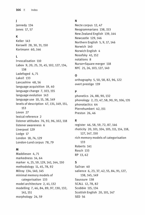
166 | Index
JJannedy 134Jones 17, 57
KKeller 143Kerswill 28, 30, 31, 150Kortmann 60, 146
Ll=vocalisation 110Labov 9, 20, 25, 31, 45, 102, 127, 134,
138Ladefoged 4, 71Lakoff 133Lancashire 48, 56language acquisition 19, 40language change 7, 103, 155language evolution 143language use 10, 15, 38, 149levels of description 47, 131, 149, 151,
153Levon 27lexical reference 2listener attitudes 76, 92, 96, 102, 118listener awareness 6Liverpool 129Lodge 17London 18, 74, 129London-Lund corpus 78, 79
MMaddieson 4, 71markedness 14, 64marker 4, 25, 59, 129, 141, 144, 150methodology 11, 45, 78, 92Milroy 134, 140, 145minimal memory models of
categorisation 133model architecture 2, 41, 132modelling 7, 46, 84, 89, 97, 130, 132,
141, 151morphology 24, 59
NNecte corpus 12, 47Neogrammarians 138, 153New Zealand English 139, 144Newcastle 129, 146Northern English 5, 9, 17, 146Norwich 140Norwich English 4Nosofsky 41, 152notations 8Nurse=Square merger 118NYC 21, 26, 103, 127, 140
Oorthography 5, 50, 58, 82, 96, 122overt prestige 139
Pphonetics 24, 88, 90, 132phonology 2, 23, 47, 58, 90, 91, 106, 135phonotactics 64Pierrehumbert 42, 151Preston 26, 46
Rregister 46, 58, 59, 72, 87, 146rhoticity 20, 101, 104, 105, 111, 114, 118,
127, 147, 150rich memory models of categorisation
133Roberts 141Rosch 133RP 13, 62
SSaffran 40salience 6, 23, 37, 42, 55, 84, 91, 127,
138, 145, 149Saussure 138SCALL 12, 78, 82Scobbie 115, 134Scottish English 20, 101, 147SED 56
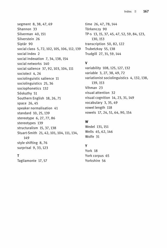
Index | 167
segment 8, 38, 47, 69Shannon 33Silverman 40, 151Silverstein 26Siptár 90social class 5, 72, 102, 105, 106, 112, 139social index 2social indexation 7, 34, 138, 154social networks 140social salience 37, 92, 103, 104, 111sociolect 4, 26sociolinguistic salience 11sociolinguistics 25, 36sociophonetics 132Sóskuthy 51Southern English 18, 26, 71space 26, 45speaker normalisation 41standard 10, 25, 139stereotype 6, 27, 77, 86stereotypes 139structuralism 15, 37, 138Stuart-Smith 21, 42, 101, 104, 111, 134,
149style shifting 8, 76surprisal 9, 33, 123
TTagliamonte 17, 57
time 26, 47, 78, 144Törkenczy 90TP-s 13, 15, 37, 45, 47, 52, 59, 84, 123,
130, 153transcription 50, 82, 122Trubetzkoy 55, 138Trudgill 27, 31, 59, 144
Vvariability 108, 125, 127, 132variable 3, 27, 38, 49, 72variationist sociolinguistics 4, 132, 138,
139, 153Vihman 23visual attention 32visual cognition 14, 23, 31, 149vocabulary 3, 35, 49vowel length 118vowels 17, 24, 51, 64, 90, 154
WWedel 131, 151Wells 45, 62, 146Wolfe 31
YYork 18York corpus 65Yorkshire 56