Topics in AI (CPSC 532S)
72
Lecture 8: Word2Vec, Language Models and RNNs Topics in AI (CPSC 532S): Multimodal Learning with Vision, Language and Sound
Transcript of Topics in AI (CPSC 532S)
Lecture 8: Word2Vec, Language Models and RNNs
Topics in AI (CPSC 532S): Multimodal Learning with Vision, Language and Sound

Course Logistics
— Assignment 3 — Final project group Goolge form will be out tomorrow

Representing a Word: One Hot Encoding
dog cat person holding tree computer using
1 2 3 4 5 6 7
one-hot encodings
[ 1, 0, 0, 0, 0, 0, 0, 0, 0, 0 ] [ 0, 1, 0, 0, 0, 0, 0, 0, 0, 0 ] [ 0, 0, 1, 0, 0, 0, 0, 0, 0, 0 ] [ 0, 0, 0, 1, 0, 0, 0, 0, 0, 0 ] [ 0, 0, 0, 0, 1, 0, 0, 0, 0, 0 ] [ 0, 0, 0, 0, 0, 1, 0, 0, 0, 0 ] [ 0, 0, 0, 0, 0, 0, 1, 0, 0, 0 ]
Vocabulary
*slide from V. Ordonex
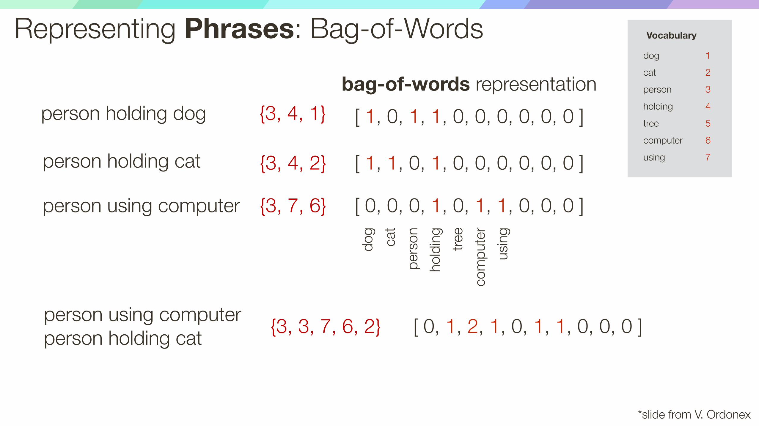
Representing Phrases: Bag-of-Wordsdog cat person holding tree computer using
1 2 3 4 5 6 7
Vocabulary
bag-of-words representation
dog
ca
t pe
rson
ho
lding
tre
e co
mpu
ter
using
person holding dog {3, 4, 1} [ 1, 0, 1, 1, 0, 0, 0, 0, 0, 0 ]
person holding cat {3, 4, 2} [ 1, 1, 0, 1, 0, 0, 0, 0, 0, 0 ]
person using computer {3, 7, 6} [ 0, 0, 0, 1, 0, 1, 1, 0, 0, 0 ]
person using computer person holding cat {3, 3, 7, 6, 2} [ 0, 1, 2, 1, 0, 1, 1, 0, 0, 0 ]
*slide from V. Ordonex

Distributional Hypothesis
— At least certain aspects of the meaning of lexical expressions depend on their distributional properties in the linguistic contexts — The degree of semantic similarity between two linguistic expressions is a function of the similarity of the two linguistic contexts in which they can appear
* Adopted from slides by Louis-Philippe Morency
[ Lenci, 2008 ]

What is the meaning of “bardiwac”?
— He handed her glass of bardiwac. — Beef dishes are made to complement the bardiwacs. — Nigel staggered to his feet, face flushed from too much bardiwac. — Malbec, one of the lesser-known bardiwac grapes, responds well to Australia’s sunshine. — I dined off bread and cheese and this excellent bardiwac. —The drinks were delicious: blood-red bardiwac as well as light, sweet Rhenish.
* Adopted from slides by Louis-Philippe Morency
bardic is an alcoholic beverage made from grapes
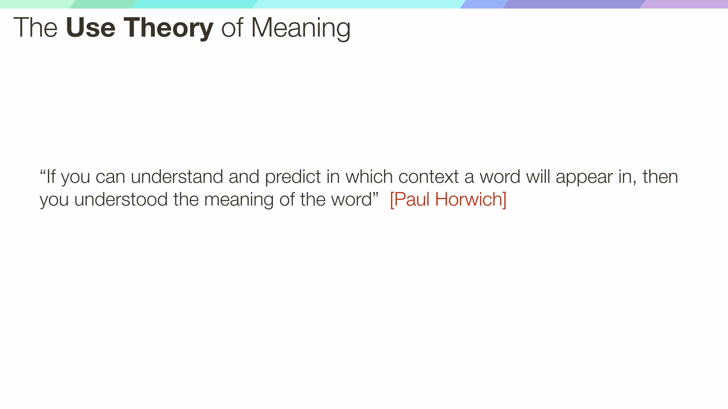
The Use Theory of Meaning
“If you can understand and predict in which context a word will appear in, then you understood the meaning of the word” [Paul Horwich]

Geometric Interpretation: Co-occurrence as feature
— Row vector describes usage of word in a corpus of text
— Can be seen as coordinates o the point in an n-dimensional Euclidian space
Co-occurrence Matrix
* Slides from Louis-Philippe Morency

Distance and Similarity
— Illustrated in two dimensions
— Similarity = spatial proximity (Euclidian distance)
— Location depends on frequency of noun (dog is 27 times as frequent as ca)
* Slides from Louis-Philippe Morency

Angle and Similarity
— direction is more important than location
— normalize length of vectors
— or use angle as a distance measure
* Slides from Louis-Philippe Morency

Geometric Interpretation: Co-occurrence as feature
— Row vector describes usage of word in a corpus of text
— Can be seen as coordinates of the point in an n-dimensional Euclidian space
Co-occurrence Matrix
* Slides from Louis-Philippe Morency
Way too high dimensional!

SVD for Dimensionality Reduction
*slide from Vagelis Hristidis

Learned Word Vector Visualization We can also use other methods, like LLE here:
[ Roweis and Saul, 2000 ]

Issues with SVD
Computational cost for a matrix is , where — Makes it not possible for large number of word vocabularies or documents
It is hard to incorporate out of sample (new) words or documents
d⇥ n O(dn2) d < n
*slide from Vagelis Hristidis

word2vec: Representing the Meaning of WordsKey idea: Predict surrounding words of every word
Benefits: Faster and easier to incorporate new document, words, etc.
*slide from Vagelis Hristidis
[ Mikolov et al., 2013 ]

word2vec: Representing the Meaning of WordsKey idea: Predict surrounding words of every word
Benefits: Faster and easier to incorporate new document, words, etc.
Continuous Bag of Words (CBOW): use context words in a window to predict middle word
Skip-gram: use the middle word to predict surrounding ones in a window*slide from Vagelis Hristidis
[ Mikolov et al., 2013 ]

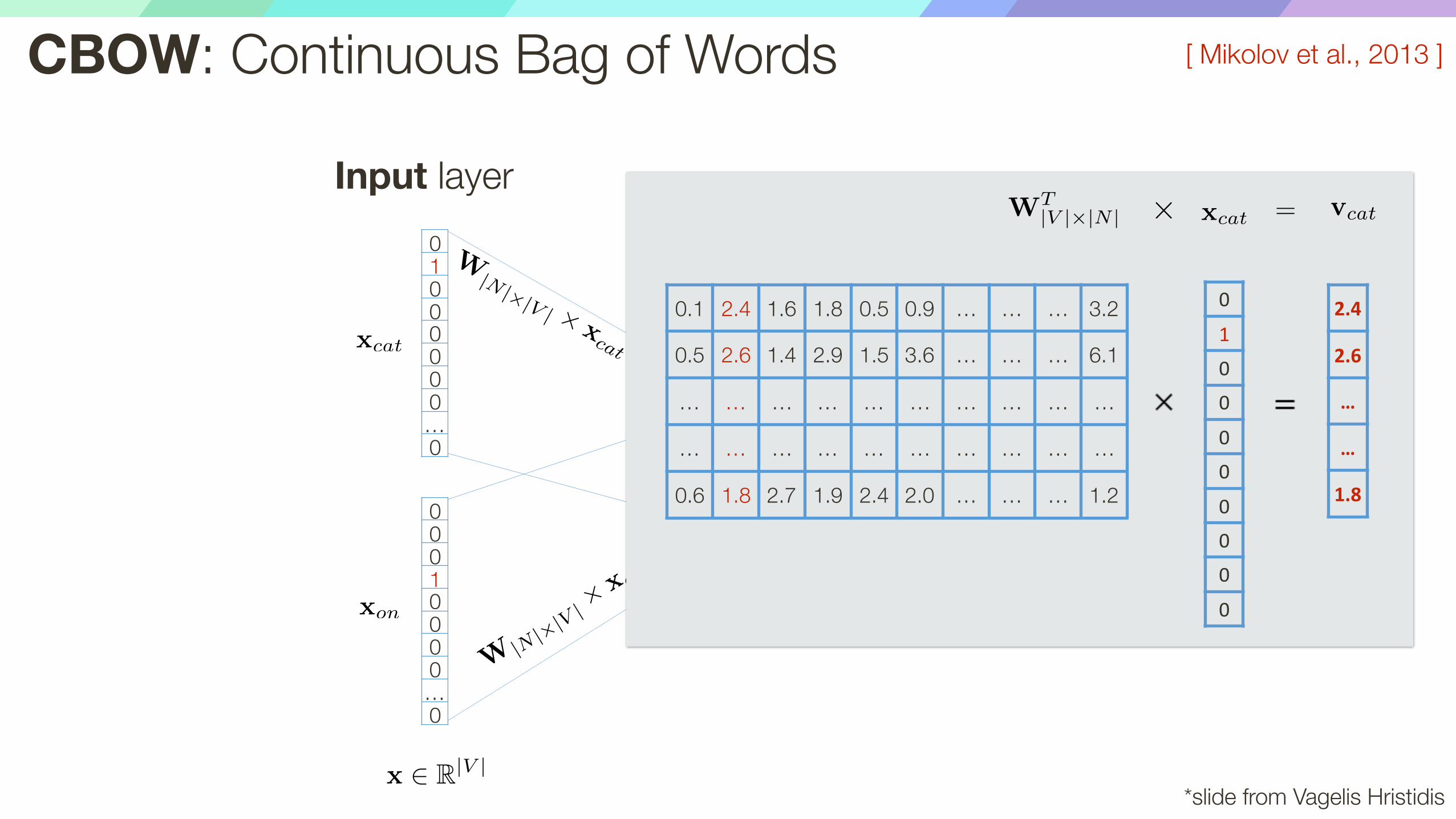
CBOW: Continuous Bag of Words
Example: “The cat sat on floor” (window size 2)
the
cat
on
floor
sat
*slide from Vagelis Hristidis
[ Mikolov et al., 2013 ]

cat
on
Input layer
Hidden layer
sat
Output layer
(one-hot vector)
01000000…0
00010000…0
00000001…0
(one-hot vector)
CBOW: Continuous Bag of Words
*slide from Vagelis Hristidis
[ Mikolov et al., 2013 ]

cat
on
Input layer
Hidden layer
sat
Output layer
01000000…0
00010000…0
00000001…0
CBOW: Continuous Bag of Words
x 2 R|V |
W|V |⇥|N |
W|V |⇥|N |
W0|N |⇥|V |
y 2 R|V |v 2 R|N |
*slide from Vagelis Hristidis
[ Mikolov et al., 2013 ]

cat
on
Input layer
Hidden layer
sat
Output layer
01000000…0
00010000…0
00000001…0
CBOW: Continuous Bag of Words
x 2 R|V |
W|V |⇥|N |
W|V |⇥|N |
W0|N |⇥|V |
y 2 R|V |v 2 R|N |
Parameters to be learned
*slide from Vagelis Hristidis
[ Mikolov et al., 2013 ]

cat
on
Input layer
Hidden layer
sat
Output layer
01000000…0
00010000…0
00000001…0
CBOW: Continuous Bag of Words
x 2 R|V |
W|V |⇥|N |
W|V |⇥|N |
W0|N |⇥|V |
y 2 R|V |v 2 R|N |
Parameters to be learned
Size of the word vector (e.g., 300)*slide from Vagelis Hristidis
[ Mikolov et al., 2013 ]

Input layer
Hidden layer
sat
Output layer
01000000…0
00010000…0
00000001…0
CBOW: Continuous Bag of Words
x 2 R|V |
y 2 R|V |v 2 R|N |
W
|N |⇥|V | ⇥x
cat =v
cat
W
|N|⇥|V |⇥
x
o
n
=v
o
n
x
on
xcat
*slide from Vagelis Hristidis
[ Mikolov et al., 2013 ]
W
|N |⇥|V | ⇥x
cat =v
cat
W
|N|⇥|V |⇥
x
o
n
=v
o
n
x
on
xcat
Input layer
Hidden layer
sat
Output layer
01000000…0
00010000…0
00000001…0
CBOW: Continuous Bag of Words
x 2 R|V |
W0|N |⇥|V |
y 2 R|V |v 2 R|N |
0.1 2.4 1.6 1.8 0.5 0.9 … … … 3.2
0.5 2.6 1.4 2.9 1.5 3.6 … … … 6.1
… … … … … … … … … …
… … … … … … … … … …
0.6 1.8 2.7 1.9 2.4 2.0 … … … 1.2
2.4
2.6
…
…
1.8
0
1
0
0
0
0
0
0
0
0
WT|V |⇥|N | xcat vcat=⇥
*slide from Vagelis Hristidis
[ Mikolov et al., 2013 ]

W
|N |⇥|V | ⇥x
cat =v
cat
W
|N|⇥|V |⇥
x
o
n
=v
o
n
x
on
xcat
Input layer
Hidden layer
sat
Output layer
01000000…0
00010000…0
00000001…0
CBOW: Continuous Bag of Words
x 2 R|V |
W0|N |⇥|V |
y 2 R|V |v 2 R|N |
0.1 2.4 1.6 1.8 0.5 0.9 … … … 3.2
0.5 2.6 1.4 2.9 1.5 3.6 … … … 6.1
… … … … … … … … … …
… … … … … … … … … …
0.6 1.8 2.7 1.9 2.4 2.0 … … … 1.2
1.8
2.9
…
…
1.9
0
0
0
1
0
0
0
0
0
0
WT|V |⇥|N | =⇥ v
on
x
on
*slide from Vagelis Hristidis
[ Mikolov et al., 2013 ]

W
|N |⇥|V | ⇥x
cat =v
cat
W
|N|⇥|V |⇥
x
o
n
=v
o
n
x
on
xcat
Input layer
Hidden layer
sat
Output layer
01000000…0
00010000…0
00000001…0
CBOW: Continuous Bag of Words
x 2 R|V |
y 2 R|V |v 2 R|N |
v =vcat
+ von
2
*slide from Vagelis Hristidis
[ Mikolov et al., 2013 ]

W
|N |⇥|V | ⇥x
cat =v
cat
W
|N|⇥|V |⇥
x
o
n
=v
o
n
x
on
xcat
Input layer
Hidden layer Output layer
01000000…0
00010000…0
00000001…0
CBOW: Continuous Bag of Words
x 2 R|V |
y 2 R|V |v 2 R|N |
W
0|V |⇥|N | ⇥ v = z
y = softmax(z)
W
0|V |⇥|N | ⇥ v = z
y = softmax(z)
ysat
0.010.020.000.020.010.020.010.7…0.00
Optimize to get close to 1-hot encoding *slide from Vagelis Hristidis
[ Mikolov et al., 2013 ]

W
|N |⇥|V | ⇥x
cat =v
cat
W
|N|⇥|V |⇥
x
o
n
=v
o
n
x
on
xcat
Input layer
Hidden layer Output layer
01000000…0
00010000…0
00000001…0
CBOW: Continuous Bag of Words
x 2 R|V |
y 2 R|V |v 2 R|N |
W
0|V |⇥|N | ⇥ v = z
y = softmax(z)
W
0|V |⇥|N | ⇥ v = z
y = softmax(z)
ysat
0.1 2.4 1.6 1.8 0.5 0.9 … … … 3.2
0.5 2.6 1.4 2.9 1.5 3.6 … … … 6.1
… … … … … … … … … …
… … … … … … … … … …
0.6 1.8 2.7 1.9 2.4 2.0 … … … 1.2
WT|V |⇥|N |
Word vectors
*slide from Vagelis Hristidis
[ Mikolov et al., 2013 ]
W
|N |⇥|V | ⇥x
cat =v
cat
W
|N|⇥|V |⇥
x
o
n
=v
o
n
x
on
xcat
Input layer
Hidden layer Output layer
01000000…0
00010000…0
00000001…0
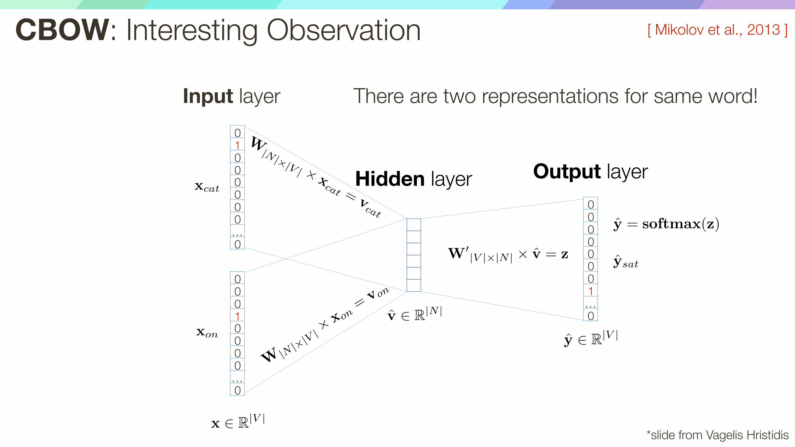
CBOW: Interesting Observation
x 2 R|V |
y 2 R|V |v 2 R|N |
W
0|V |⇥|N | ⇥ v = z
y = softmax(z)
W
0|V |⇥|N | ⇥ v = z
y = softmax(z)
ysat
*slide from Vagelis Hristidis
[ Mikolov et al., 2013 ]
There are two representations for same word!

p(w|c) =exp
h(
Pc Wxc)
T(Wxw)
i
P|V |i exp
h(Wxi)
T(Wxw)
i
CBOW: Interesting Observation [ Mikolov et al., 2013 ]
Another way to look at it: Maximize similarity between context word representation and the word representation itself

J(W) = � 1
T
TX
t=1
X
�mjm;j 6=0
log p(wt+j |wt)
p(wt+j |wt) =exp(wT
t+jwt)
P|V |i=1 exp(w
Ti wt)
CBOW: Interesting Observation
Another way to look at it: Maximize similarity between context word representation and the word representation itself
[ Mikolov et al., 2013 ]

Skip-Gram Model [ Mikolov et al., 2013 ]

Comparison
— CBOW is not great for rare words and typically needs less data to train — Skip-gram better for rate words and needs more data to train the model
[ Mikolov et al., 2013 ]
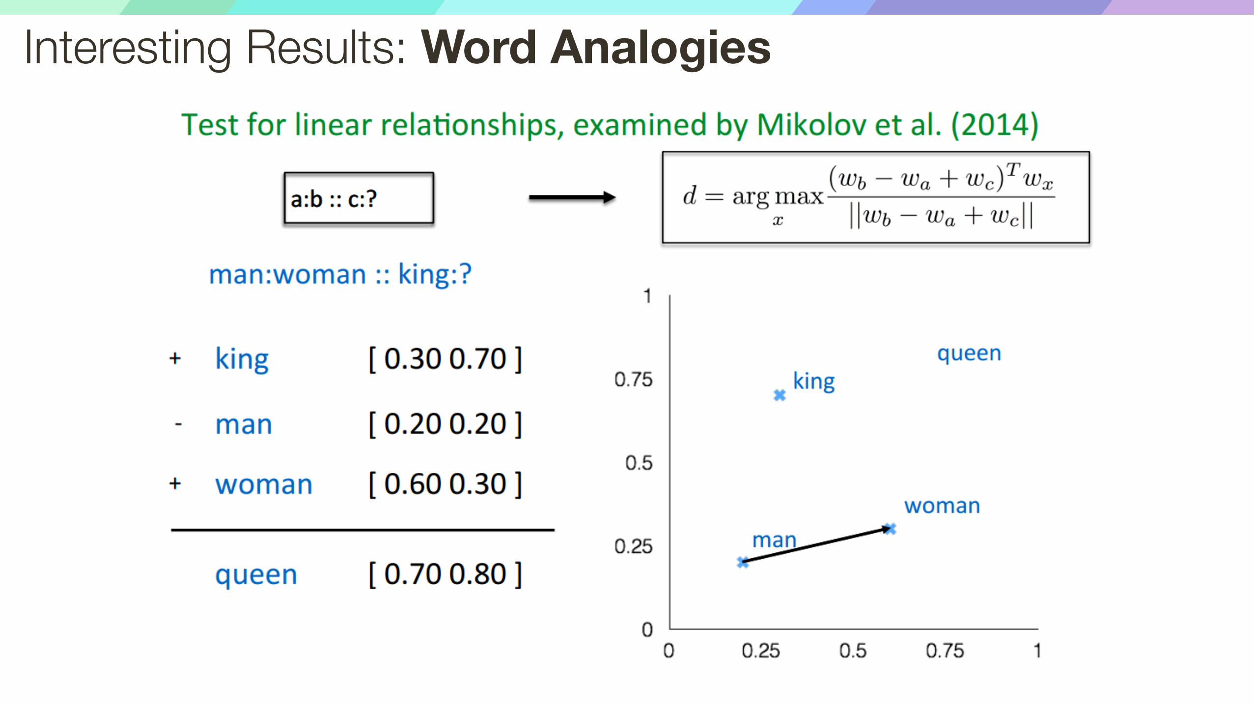
Interesting Results: Word Analogies

Interesting Results: Word Analogies [ Mikolov et al., 2013 ]
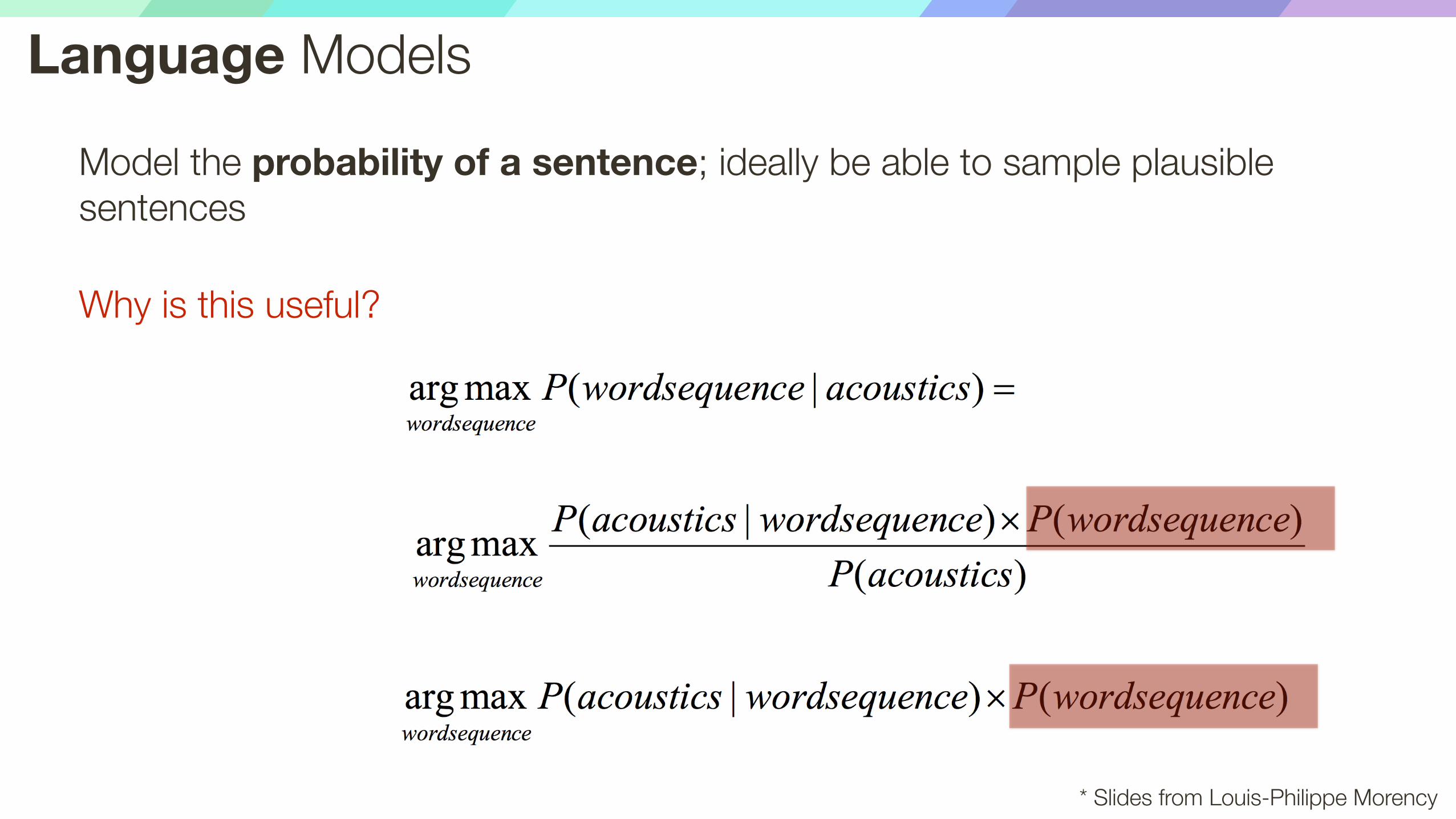
Language Models
Model the probability of a sentence; ideally be able to sample plausible sentences
Why is this useful?
* Slides from Louis-Philippe Morency

Simple Language Models: N-Gramsw1:n = [w1, w2, ..., wn]
p(w1:n) = p(w1)p(w2|w1)p(w3|w1, w2) · · · p(wn|w1:n�1)
Given a word sequence:
We want to estimate
p(w1:n) = p(w1)p(w2|w1)p(w3|w1, w2) · · · p(wn|w1:n�1)
Using Chain Rule of probabilities:
p(w1:n) =nY
k=1
p(wk|wk�1) p(w1:n) =nY
k=1
p(wk|wk�N+1:k�1)
Bi-gram Approximation: N-gram Approximation:
* Slides from Louis-Philippe Morency

Estimating Probabilities
p(wn|wn�1) =C(wn�1wn)
C(wn�1)
p(wn|wn�N�1:n�1) =C(wn�N�1:n�1wn)
C(wn�N�1:n�1)
N-gram conditional probabilities can be estimated based on raw concurrence counts in the observed sequences
Bi-gram:
N-gram:
* Slides from Louis-Philippe Morency

Neural-based Unigram Language Mode
* Slides from Louis-Philippe Morency
Problem: Does not model sequential information (too local)
We need sequence modeling!

Sequence Modeling

Why Model Sequences?
* slide from Dhruv BatraImage Credit: Alex Graves and Kevin Gimpel

Multi-modal tasks
Cap$onGenera$on:Vinyalsetal.2015
[ Vinyals et al., 2015 ]

Sequences where you don’t expect them …
Classify images by taking a series of “glimpses”
[ Gregor et al., ICML 2015 ][ Mnih et al., ICLR 2015 ]
* slide from Fei-Dei Li, Justin Johnson, Serena Yeung, cs231n Stanford

Sequences in Inputs or Outputs?
Input: No sequence Output: No seq.
Example: “standard”
classification / regression problems
* slide from Fei-Dei Li, Justin Johnson, Serena Yeung, cs231n Stanford

Sequences in Inputs or Outputs?
Input: No sequence Output: No seq.
Example: “standard”
classification / regression problems
Input: No sequence Output:
Sequence Example:
Im2Caption
* slide from Fei-Dei Li, Justin Johnson, Serena Yeung, cs231n Stanford

Sequences in Inputs or Outputs?
Input: No sequence Output: No seq.
Example: “standard”
classification / regression problems
Input: No sequence Output:
Sequence Example:
Im2Caption
Input: Sequence Output: No seq.
Example: sentence classification,
multiple-choice question answering
Input: Sequence Output: Sequence
Example: machine translation, video captioning, open-ended question answering, video question
answering
* slide from Fei-Dei Li, Justin Johnson, Serena Yeung, cs231n Stanford

Key Conceptual Ideas
Parameter Sharing
— in computational graphs = adding gradients
“Unrolling” — in computational graphs with parameter sharing
Parameter Sharing + “Unrolling” — Allows modeling arbitrary length sequences! — Keeps number of parameters in check
* slide from Dhruv Batra
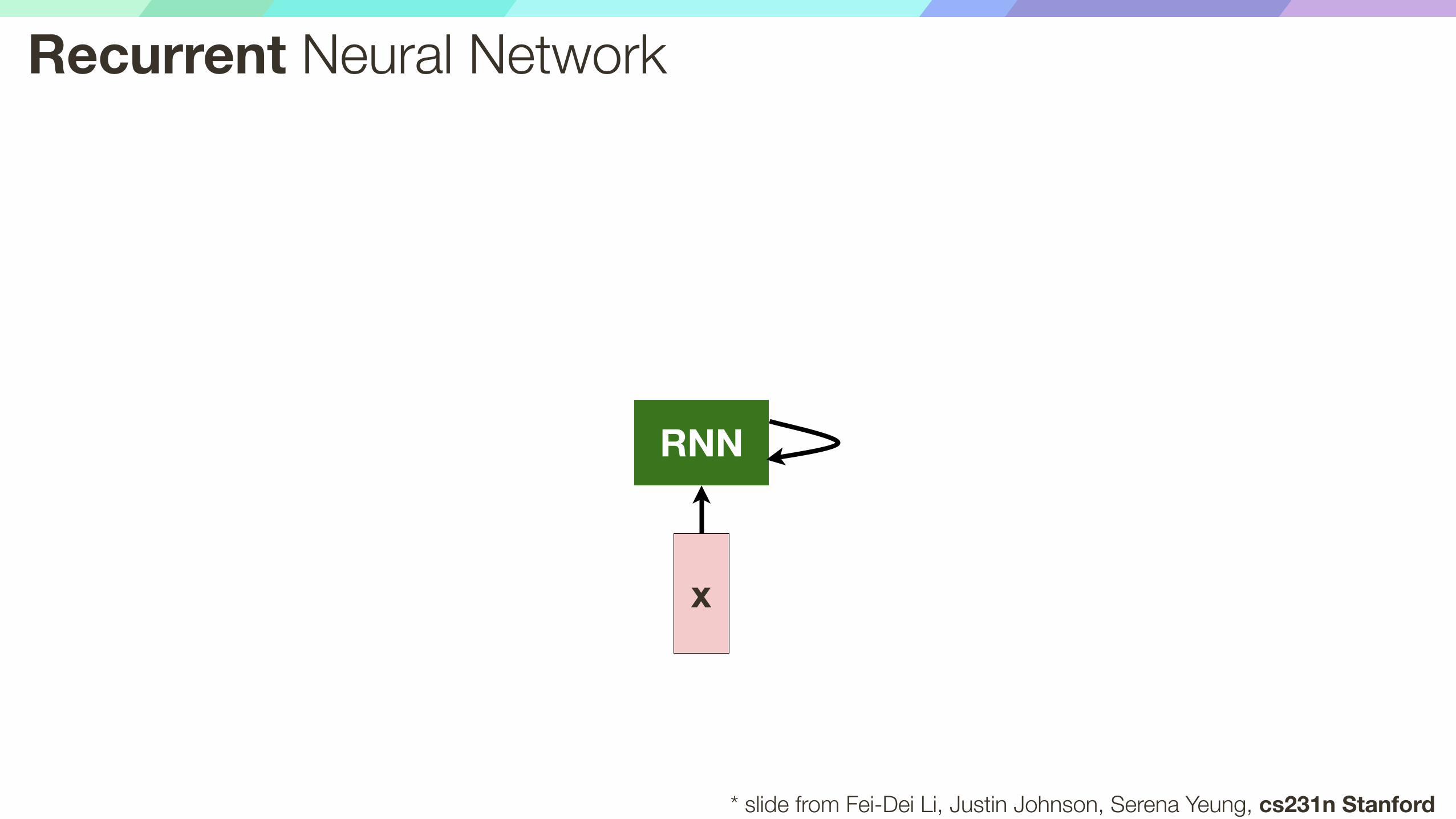
x
RNN
Recurrent Neural Network
* slide from Fei-Dei Li, Justin Johnson, Serena Yeung, cs231n Stanford
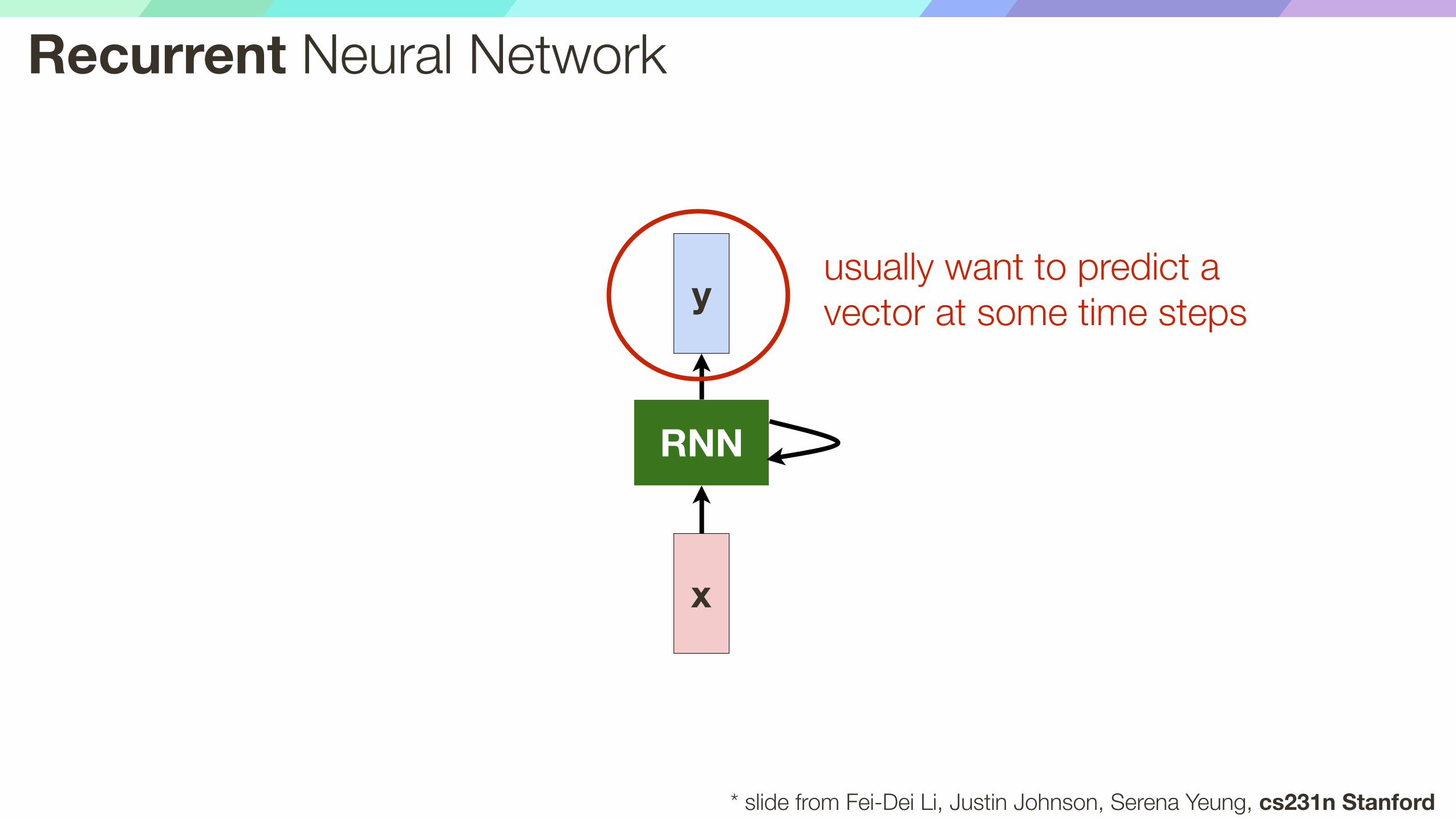
x
RNN
yusually want to predict a vector at some time steps
Recurrent Neural Network
* slide from Fei-Dei Li, Justin Johnson, Serena Yeung, cs231n Stanford
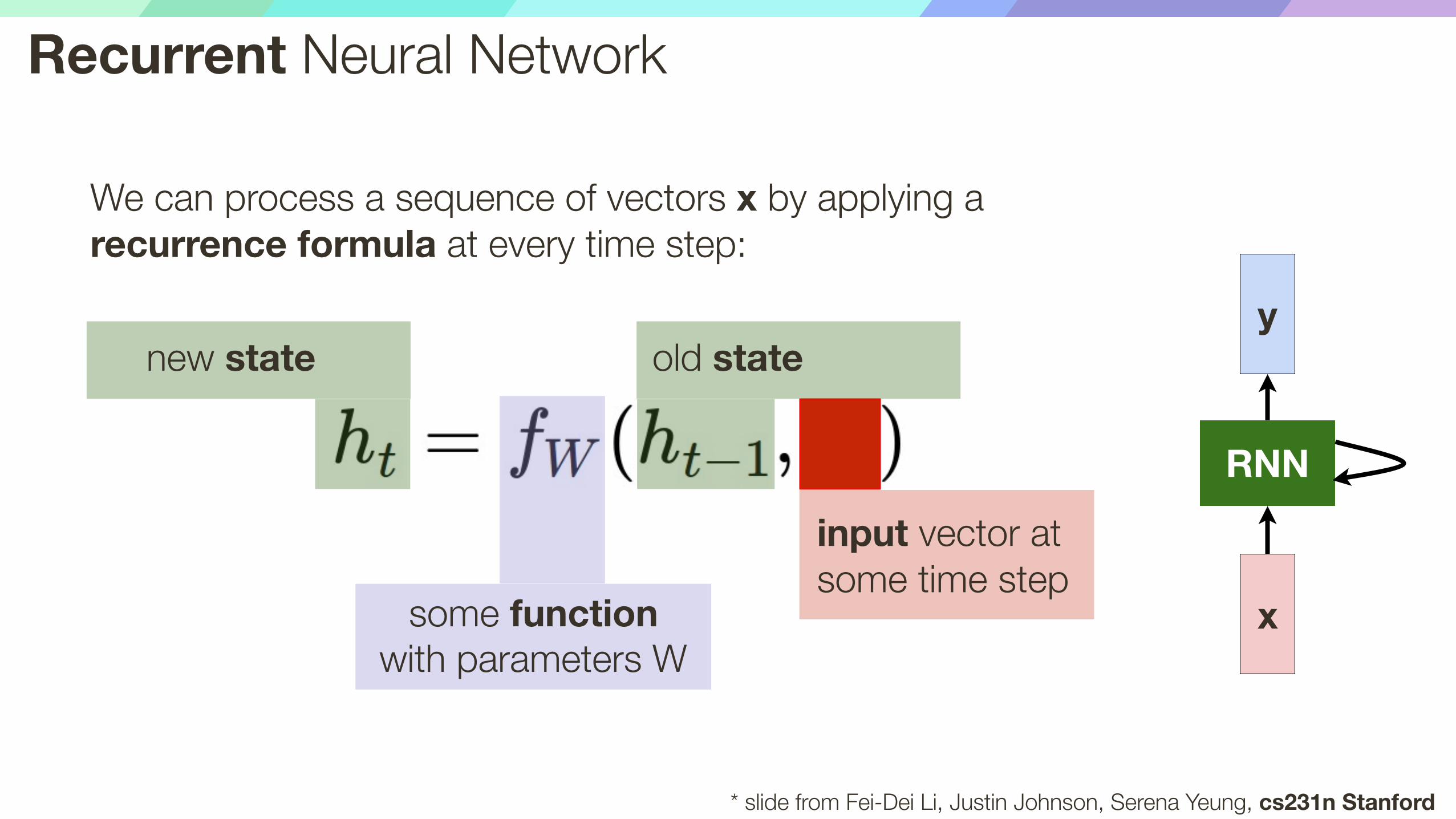
Recurrent Neural Network
We can process a sequence of vectors x by applying a recurrence formula at every time step:
some function with parameters W
x
RNN
y
input vector at some time step
old statenew state
* slide from Fei-Dei Li, Justin Johnson, Serena Yeung, cs231n Stanford

Recurrent Neural Network
We can process a sequence of vectors x by applying a recurrence formula at every time step:
x
RNN
y
Note: the same function and the same set of parameters are used at every time step
* slide from Fei-Dei Li, Justin Johnson, Serena Yeung, cs231n Stanford

(Vanilla) Recurrent Neural Network
x
RNN
y
* slide from Fei-Dei Li, Justin Johnson, Serena Yeung, cs231n Stanford

RNN Computational Graph
h0 fW h1
x1
* slide from Fei-Dei Li, Justin Johnson, Serena Yeung, cs231n Stanford

RNN Computational Graph
h0 fW h1 fW h2
x2x1
* slide from Fei-Dei Li, Justin Johnson, Serena Yeung, cs231n Stanford

RNN Computational Graph
h0 fW h1 fW h2 fW h3
x3
…
x2x1
hT
* slide from Fei-Dei Li, Justin Johnson, Serena Yeung, cs231n Stanford

RNN Computational Graph
h0 fW h1 fW h2 fW h3
x3
…
x2x1W
hT
Re-use the same weight matrix at every time-step
* slide from Fei-Dei Li, Justin Johnson, Serena Yeung, cs231n Stanford

RNN Computational Graph: Many to Many
h0 fW h1 fW h2 fW h3
x3
yT
…
x2x1W
hT
y3y2y1
* slide from Fei-Dei Li, Justin Johnson, Serena Yeung, cs231n Stanford

RNN Computational Graph: Many to Many
h0 fW h1 fW h2 fW h3
x3
yT
…
x2x1W
hT
y3y2y1 L1 L2 L3 LT
* slide from Fei-Dei Li, Justin Johnson, Serena Yeung, cs231n Stanford

RNN Computational Graph: Many to Many
h0 fW h1 fW h2 fW h3
x3
yT
…
x2x1W
hT
y3y2y1 L1 L2 L3 LT
L
* slide from Fei-Dei Li, Justin Johnson, Serena Yeung, cs231n Stanford

RNN Computational Graph: Many to One
h0 fW h1 fW h2 fW h3
x3
y
…
x2x1W
hT
* slide from Fei-Dei Li, Justin Johnson, Serena Yeung, cs231n Stanford

RNN Computational Graph: One to Many
h0 fW h1 fW h2 fW h3
yT
…
xW
hT
y3y2y1
* slide from Fei-Dei Li, Justin Johnson, Serena Yeung, cs231n Stanford

Sequence to Sequence: Many to One + One to Many
h0 fW h1 fW h2 fW h3
x3
…
x2x1W1
hT
Many to one: Encode input sequence in a single vector
y1 y2
fW h1 fW h2 fW
W2
One to many: Produce output sequence from single input vector
* slide from Fei-Dei Li, Justin Johnson, Serena Yeung, cs231n Stanford

Example: Character-level Language Model
Vocabulary: [‘h’, ‘e’, ‘l’, ‘o’]
Example training sequence: “hello”
* slide from Fei-Dei Li, Justin Johnson, Serena Yeung, cs231n Stanford

Example: Character-level Language Model
Vocabulary: [‘h’, ‘e’, ‘l’, ‘o’]
Example training sequence: “hello”
* slide from Fei-Dei Li, Justin Johnson, Serena Yeung, cs231n Stanford

Example: Character-level Language Model
Vocabulary: [‘h’, ‘e’, ‘l’, ‘o’]
Example training sequence: “hello”
* slide from Fei-Dei Li, Justin Johnson, Serena Yeung, cs231n Stanford

Example: Character-level Language Model (Sampling)
Vocabulary: [‘h’, ‘e’, ‘l’, ‘o’]
At test time sample one character at a time and feed back to the model
.03
.13
.00
.84
.25
.20
.05
.50
.11
.17
.68
.03
.11
.02.08
.79Softmax
“e” “l” “l” “o”Sample
* slide from Fei-Dei Li, Justin Johnson, Serena Yeung, cs231n Stanford
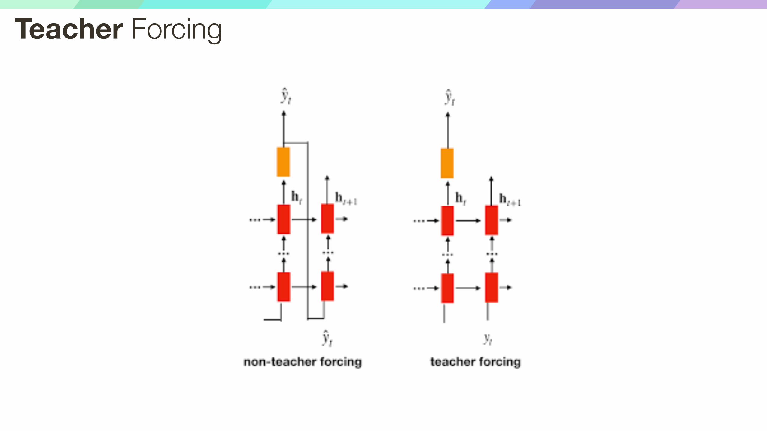
Teacher Forcing

Sampling vs. ArgMax
.03
.13
.00
.84
.25
.20
.05
.50
.11
.17
.68
.03
.11
.02.08
.79Softmax
“e” “l” “l” “o”Sample
Sampling: allows to generate diverse outputs
ArgMax: could be more stable in practice