TopicModel4J: A Java Package for Topic Models
52
TopicModel4J: A Java Package for Topic Models Yang Qian Hefei University of Technology Yuanchun Jiang * Hefei University of Technology Yidong Chai Hefei University of Technology Yezheng Liu Hefei University of Technology Jianshan Sun Hefei University of Technology Abstract Topic models provide a flexible and principled framework for exploring hidden struc- ture in high-dimensional co-occurrence data and are commonly used natural language processing (NLP) of text. In this paper, we design and implement a Java package, Top- icModel4J, which contains 13 kinds of representative algorithms for fitting topic models. The TopicModel4J in the Java programming environment provides an easy-to-use inter- face for data analysts to run the algorithms, and allow to easily input and output data. In addition, this package provides a few unstructured text preprocessing techniques, such as splitting textual data into words, lowercasing the words, preforming lemmatization and removing the useless characters, URLs and stop words. Keywords : natural language processing, topic model, Gibbs sampling, variational inference, Java. 1. Introduction Topic models are a type of probabilistic generative models which are widely used to discover latent semantics (e.g., topics) from a large collection of documents. Based upon the intuition that one document can be represented as an admixture of abstract topics and one topic is a set of similar vocabulary words, topic models can find word patterns, abstract topics and topics that best characterize each document in an unsupervised manner. Therefore, topic models can provide insights for us to understand collections of documents, or any other data types as long as they can be treated as documents (e.g., images, networks, and genetic information). * Corresponding author. E-mail address: [email protected] arXiv:2010.14707v1 [cs.CL] 28 Oct 2020
Transcript of TopicModel4J: A Java Package for Topic Models

TopicModel4J: A Java Package for Topic Models
Yang QianHefei University of Technology
Yuanchun Jiang∗Hefei University of Technology
Yidong ChaiHefei University of Technology
Yezheng LiuHefei University of Technology
Jianshan SunHefei University of Technology
Abstract
Topic models provide a flexible and principled framework for exploring hidden struc-ture in high-dimensional co-occurrence data and are commonly used natural languageprocessing (NLP) of text. In this paper, we design and implement a Java package, Top-icModel4J, which contains 13 kinds of representative algorithms for fitting topic models.The TopicModel4J in the Java programming environment provides an easy-to-use inter-face for data analysts to run the algorithms, and allow to easily input and output data. Inaddition, this package provides a few unstructured text preprocessing techniques, such assplitting textual data into words, lowercasing the words, preforming lemmatization andremoving the useless characters, URLs and stop words.
Keywords: natural language processing, topic model, Gibbs sampling, variational inference,Java.
1. IntroductionTopic models are a type of probabilistic generative models which are widely used to discoverlatent semantics (e.g., topics) from a large collection of documents. Based upon the intuitionthat one document can be represented as an admixture of abstract topics and one topic is a setof similar vocabulary words, topic models can find word patterns, abstract topics and topicsthat best characterize each document in an unsupervised manner. Therefore, topic modelscan provide insights for us to understand collections of documents, or any other data types aslong as they can be treated as documents (e.g., images, networks, and genetic information).
∗Corresponding author. E-mail address: [email protected]
arX
iv:2
010.
1470
7v1
[cs
.CL
] 2
8 O
ct 2
020
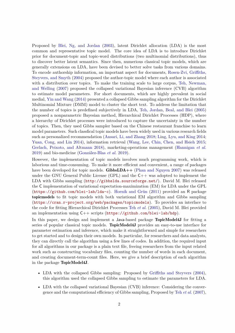
Proposed by Blei, Ng, and Jordan (2003), latent Dirichlet allocation (LDA) is the mostcommon and representative topic model. The core idea of LDA is to introduce Dirichletprior for document-topic and topic-word distributions (two multinomial distributions), thusto discover better latent semantics. Since then, numerious classical topic models, which aregenerally extensions on LDA, have been devised to better solve tasks from various domains.To encode authorship information, an important aspect for documents, Rosen-Zvi, Griffiths,Steyvers, and Smyth (2004) proposed the author-topic model where each author is associatedwith a distribution over topics. To make the training scale to large corpus, Teh, Newman,and Welling (2007) proposed the collapsed variational Bayesian inference (CVB) algorithmto estimate model parameters. For short documents, which are highly prevalent in socialmedial, Yin and Wang (2014) presented a collapsed Gibbs sampling algorithm for the DirichletMultinomial Mixture (DMM) model to cluster the short text. To address the limitation thatthe number of topics is predefined subjectively in LDA, Teh, Jordan, Beal, and Blei (2005)proposed a nonparametric Bayesian method, Hierarchical Dirichlet Processes (HDP), wherea hierarchy of Dirichlet processes were introduced to capture the uncertainty in the numberof topics. Then, they used Gibbs sampler based on the Chinese restaurant franchise to learnmodel parameters. Such classfical topic models have been widely used in various research fieldssuch as personalized recommendation (Ansari, Li, and Zhang 2018; Ling, Lyu, and King 2014;Yuan, Cong, and Lin 2014), information retrieval (Wang, Lee, Chin, Chen, and Hsieh 2015;Gerlach, Peixoto, and Altmann 2018), marketing-operations management (Hannigan et al.2019) and bio-medicine (González-Blas et al. 2019).However, the implementation of topic models involves much programming work, which islaborious and time-consuming. To make it more efficient and convenient, a range of packageshave been developed for topic models. GibbsLDA++ (Phan and Nguyen 2007) was releasedunder the GNU General Public License (GPL) and the C++ was adopted to implement theLDA with Gibbs sampling (http://gibbslda.sourceforge.net/). David M. Blei releasedthe C implementation of variational expectation-maximization (EM) for LDA under the GPL(https://github.com/blei-lab/lda-c). Hornik and Grün (2011) provided an R packagetopicmodels to fit topic models with both variational EM algorithm and Gibbs sampling(https://cran.r-project.org/web/packages/topicmodels). To provides an interface tothe code for fitting Hierarchical Dirichlet Processes Teh et al. (2005), David M. Blei providedan implementation using C++ scripts (https://github.com/blei-lab/hdp).In this paper, we design and implement a Java-based package TopicModel4J for fitting aseries of popular classical topic models. TopicModel4J provides an easy-to-use interface forparameter estimation and inference, which make it straightforward and simple for researchersto get started and to design their own models. In particular, for researchers and data analysts,they can directly call the algorithm using a few lines of codes. In addition, the required inputfor all algorithms in our package is a plain text file, freeing researchers from the input relatedwork such as constructing vocabulary files, counting the number of words in each document,and creating document-term-count files. Here, we give a brief description of each algorithmin the package TopicModel4J.
• LDA with the collapsed Gibbs sampling: Proposed by Griffiths and Steyvers (2004),this algorithm used the collapsed Gibbs sampling to estimate the parameters for LDA.
• LDA with the collapsed variational Bayesian (CVB) inference: Considering the conver-gence and the computational efficiency of Gibbs sampling, Proposed by Teh et al. (2007),
2

this algorithm combined the key insights of Gibbs sampling and standard variationalinference algorithm, and then propose the CVB algorithm for inferring LDA.
• Sentence-LDA: Sentence-LDA is proposed by Jo and Oh (2011). Unlike LDA, Sentence-LDA assumes that the words in one sentences of the document is drawn from the sametopic. This algorithm is often used to analyze the unstructured online reviews (Büschkenand Allenby 2016). In the package TopicModel4J, we use collapsed Gibbs sampling forinferring the Sentence-LDA.
• HDP with Chinese restaurant franchise: HDP (Teh et al. 2005) is nonparametric ap-proach which extends the Dirichlet processes (DP) to model the uncertainty concerningthe number of topics. HDP can be inferred by Gibbs sampling based on Chinese restau-rant franchise metaphor.
• Dirichlet Multinomial Mixture (DMM) Model: DMM model (Nigam et al. 2000) as-sumes that each document is only assigned to one cluster or topic. Recently, this modelis widely used for short text clustering (Li et al. 2016; Liang et al. 2016; Yin and Wang2014). In the package TopicModel4J, we use collapsed Gibbs sampling algorithm forinferring the DMM model (Yin and Wang 2014).
• Dirichlet Process Multinomial Mixture (DPMM) model: DPMM model (Yu et al. 2010;Zhang, Ghahramani, and Yang 2005) is an extension of DMMmodel. This model is oftenused to handle the short text clustering problem. Compared with DMM, the characterof the DPMM model is that the number of clusters can be determined automatically.In our package, we use collapsed Gibbs sampling algorithm for inferring the parametersof DPMM (Yin and Wang 2016).
• Pseudo-document-based Topic Model (PTM): PTM (Zuo et al. 2016) is a short texttopic modeling, which leads into the thought of pseudo document to indirectly aggregateshort texts against the sparsity in terms of word co-occurrences. In our package, we usecollapsed Gibbs sampling algorithm for approximate inference of PTM.
• Biterm topic model (BTM): BTM (Cheng, Yan, Lan, and Guo 2014; Yan, Guo, Lan,and Cheng 2013) is a popular short text topic modeling, which introduce the word pairco-occurring in a short document to overcome the sparsity of word co-occurrence. Theword pair that is generated by the short document, is noted as ’biterm’. In our package,we conduct an approximate inference for BTM using the collapsed Gibbs samplingalgorithm.
• Author-topic model (ATM): ATM (Rosen-Zvi et al. 2004) is an extension of LDA, thatmodels the interests of authors and the documents at the same time. In our package,we use the collapsed Gibbs sampling algorithm to estimate the parameters of ATM.
• Link LDA: Link LDA (Erosheva, Fienberg, and Lafferty 2004) is originally proposedto model the documents containing abstracts and references. The references of eachdocument can be viewed as a set of links. Recently, different variants of Link LDA havebeen recently proposed to mining the topic-specific influencers [26-28]. In our package,we use collapsed Gibbs sampling algorithm to estimate the parameters of Link LDA(Su, Wang, Zhang, Chang, and Zia 2018; Bi, Tian, Sismanis, Balmin, and Cho 2014;Yang, Jin, Chi, and Zhu 2009).
3

• Labeled LDA: Labeled LDA is a supervised topic model that proposed by Ramage,Hall, Nallapati, and Manning (2009). This model is applicable for multi-labeled cor-pora. Unlike LDA, Labeled LDA defines a consistent one-to-one match between theLDA’s latent topics and the labels. Hence, this model enhances the results that can beinterpretative. In our package, we use collapsed Gibbs sampling algorithm to estimatethe parameters of Labeled LDA.
• Partially Labeled Dirichlet Allocation (PLDA): PLDA is also a supervised topic modelthat is proposed by Ramage, Manning, and Dumais (2011). This model is applicablefor multi-labeled corpora. Unlike Labeled LDA, PLDA introduce one class (containingmultiple topics) for each label in the label set. In our package, we use collapsed Gibbssampling algorithm to estimate the parameters of PLDA.
• Dual-Sparse Topic Model: This model is a sparsity-enhanced topic model, proposed byLin, Tian, Mei, and Cheng (2014). Unlike LDA, this model assumes that each documentoften concentrates on several salient topics and each topic often focus on a narrow rangeof words. In our package, we use CVB inference to estimate the parameters of the dual-sparse topic model.
The remainder of this paper is structured as follows: Section 2 reviews the related methods inTopicModel4J. In Section 3, we introduce the formula interface of each model in TopicModel4Jand give the applications on real dataset. We finally present conclusions in Section 4.
2. Models
2.1. LDA
LDA (Blei et al. 2003) is a generative statistical model that depicts how a corpus of documentsis generated by a set of latent topics. Let M denote the number of documents in a collection;V denotes the number of words in the vocabulary; K denotes the number of topics. Further,we define wm,n as the n-th word (token) in the m-th document, zm.n ∈ {1, , 2, · · · ,K} asthe topic assignment for wm,n, and Nm as number of word tokens in document m. Letθm,k denote the probability of topic k occurring in the m-th document and φk,v denote theprobability of word v occurring in topic k, then the model parameters θm = {θm,k}Kk=1 ,∀mand φk = {φk,v}Vv=1 ,∀k are defined as K-dimensional topic mixing vector and V -dimensionaltopic-word vector respectively. The generative process of LDA is described as follows:
1) For each topic k ∈ [1,K]
(a) Draw φk ∼ Dirichlet (β)
2) For each document m ∈ [1,M ]
(a) Draw θm ∼ Dirichlet (α)(b) For each word wm,n in document m, n ∈ [1, Nm]
i. Draw a topic zm,n ∼Multinomial (θm)ii. Draw a word wm,n ∼Multinomial
(φzm,n
)4
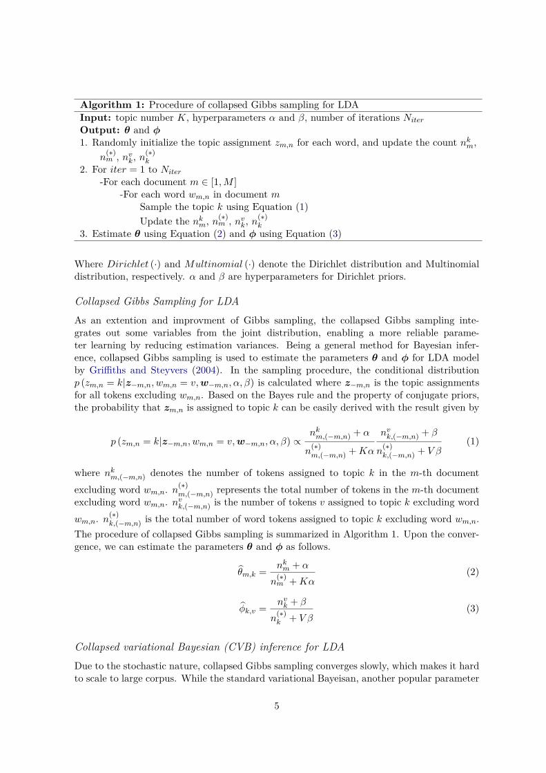
Algorithm 1: Procedure of collapsed Gibbs sampling for LDAInput: topic number K, hyperparameters α and β, number of iterations Niter
Output: θ and φ1. Randomly initialize the topic assignment zm,n for each word, and update the count nkm,
n(∗)m , nvk, n
(∗)k
2. For iter = 1 to Niter
-For each document m ∈ [1,M ]-For each word wm,n in document m
Sample the topic k using Equation (1)Update the nkm, n
(∗)m , nvk, n
(∗)k
3. Estimate θ using Equation (2) and φ using Equation (3)
Where Dirichlet (·) and Multinomial (·) denote the Dirichlet distribution and Multinomialdistribution, respectively. α and β are hyperparameters for Dirichlet priors.
Collapsed Gibbs Sampling for LDAAs an extention and improvment of Gibbs sampling, the collapsed Gibbs sampling inte-grates out some variables from the joint distribution, enabling a more reliable parame-ter learning by reducing estimation variances. Being a general method for Bayesian infer-ence, collapsed Gibbs sampling is used to estimate the parameters θ and φ for LDA modelby Griffiths and Steyvers (2004). In the sampling procedure, the conditional distributionp (zm,n = k|z−m,n, wm,n = v,w−m,n, α, β) is calculated where z−m,n is the topic assignmentsfor all tokens excluding wm,n. Based on the Bayes rule and the property of conjugate priors,the probability that zm,n is assigned to topic k can be easily derived with the result given by
p (zm,n = k|z−m,n, wm,n = v,w−m,n, α, β) ∝nkm,(−m,n) + α
n(∗)m,(−m,n) +Kα
nvk,(−m,n) + β
n(∗)k,(−m,n) + V β
(1)
where nkm,(−m,n) denotes the number of tokens assigned to topic k in the m-th documentexcluding word wm,n. n(∗)
m,(−m,n) represents the total number of tokens in the m-th documentexcluding word wm,n. nvk,(−m,n) is the number of tokens v assigned to topic k excluding wordwm,n. n(∗)
k,(−m,n) is the total number of word tokens assigned to topic k excluding word wm,n.The procedure of collapsed Gibbs sampling is summarized in Algorithm 1. Upon the conver-gence, we can estimate the parameters θ and φ as follows.
θm,k = nkm + α
n(∗)m +Kα
(2)
φk,v = nvk + β
n(∗)k + V β
(3)
Collapsed variational Bayesian (CVB) inference for LDADue to the stochastic nature, collapsed Gibbs sampling converges slowly, which makes it hardto scale to large corpus. While the standard variational Bayeisan, another popular parameter
5
learning method, can overcome this limitation, it is efficient for large scale applications.However, the standard variational Bayeisan may lead to inaccurate estimates of the posteriorcomparing with collapsed Gibbs sampling (Teh et al. (2007)). Collapsed variational Bayesian(CVB) inference for LDA combines the strengths of collapsed Gibbs sampling and standardvariational Bayesian, thus offering a more effective and efficient approach to learn modelparameters. The core idea is to simplify the evidence lower bound (ELBO) on logp (w|α, β)by marginalizing out the parameters θ and φ. Based on Teh et al. (2007), we can rewriteELBO as follows.
ELBO (q (z)) = Eq(z) [logp (w, z|α, β)]− Eq(z) [logq (z)] (4)
where p (w, z|α, β) is the marginal distribution over w and z. q (z) is the variational dis-tribution, which is approximation to true distribution p(z). According to mean-field theory,q (z) is assumed to factorize over latent variables and thus expressed as:
q (z) =M∏m=1
Nm∏n=1
q (zm,n|γm,n) (5)
where q (zm,n|γm,n) is restricted to be the Multinomial distribution parameterized by γm,n.The optimization goal is to maximize the ELBO, which is equivalent to minimize the differencebetween true posterior p(z) and the variational distribution q(z). The optimal variationalparameters γm,n,k = q (zm,n = k|γm,n) can computed by
γm,n,k =exp
(Eq(z−m,n)logp (z−m,n, zm,n = k,w|α, β)
)∑Kk′=1 exp
(Eq(z−m,n)logp (z−m,n, zm,n = k′ , w|α, β)
) (6)
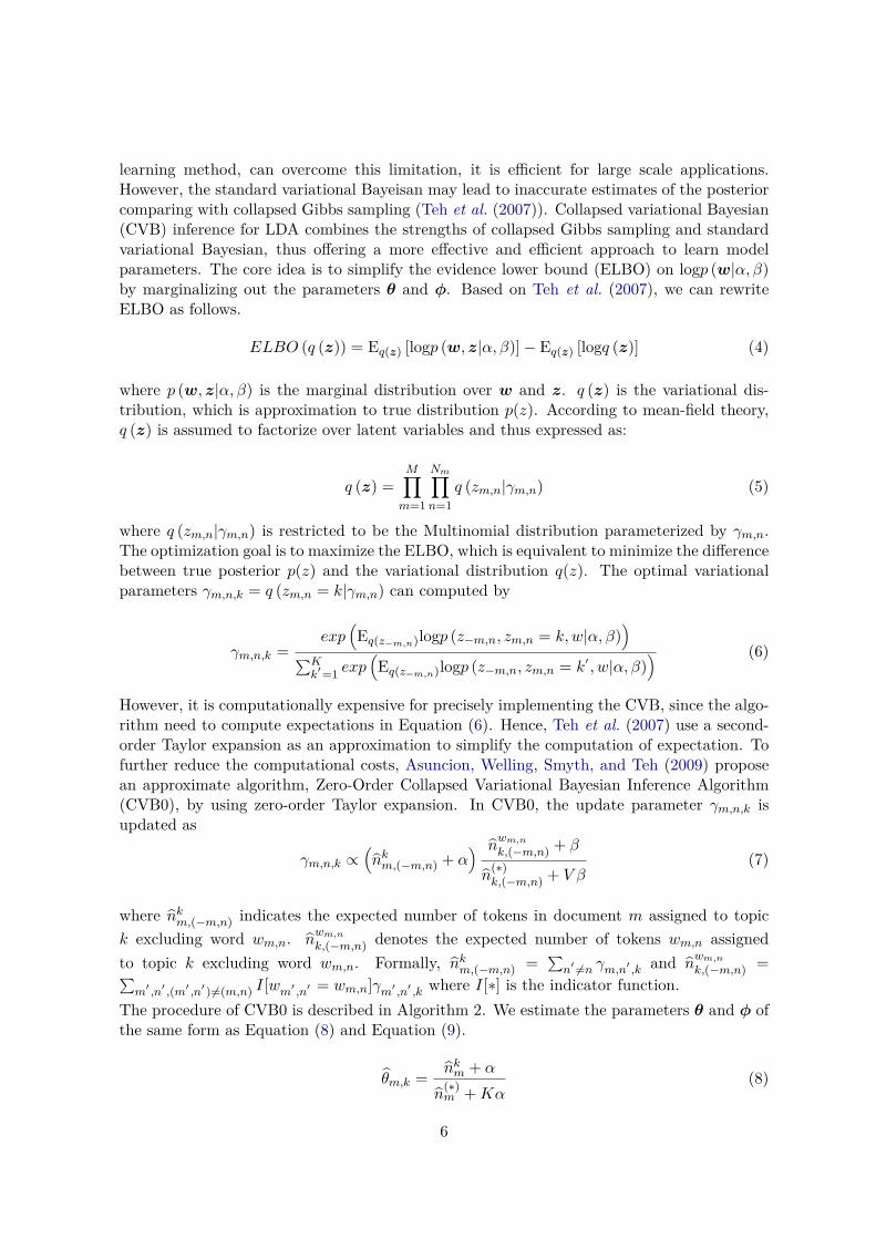
However, it is computationally expensive for precisely implementing the CVB, since the algo-rithm need to compute expectations in Equation (6). Hence, Teh et al. (2007) use a second-order Taylor expansion as an approximation to simplify the computation of expectation. Tofurther reduce the computational costs, Asuncion, Welling, Smyth, and Teh (2009) proposean approximate algorithm, Zero-Order Collapsed Variational Bayesian Inference Algorithm(CVB0), by using zero-order Taylor expansion. In CVB0, the update parameter γm,n,k isupdated as
γm,n,k ∝(nkm,(−m,n) + α
) nwm,n
k,(−m,n) + β
n(∗)k,(−m,n) + V β
(7)
where nkm,(−m,n) indicates the expected number of tokens in document m assigned to topick excluding word wm,n. n
wm,n
k,(−m,n) denotes the expected number of tokens wm,n assignedto topic k excluding word wm,n. Formally, nkm,(−m,n) =
∑n′ 6=n γm,n′ ,k and n
wm,n
k,(−m,n) =∑m′ ,n′ ,(m′ ,n′ )6=(m,n) I[wm′ ,n′ = wm,n]γm′ ,n′ ,k where I[∗] is the indicator function.
The procedure of CVB0 is described in Algorithm 2. We estimate the parameters θ and φ ofthe same form as Equation (8) and Equation (9).
θm,k = nkm + α
n(∗)m +Kα
(8)
6
Algorithm 2: Procedure of CVB0 for LDAInput: topic number K, hyperparameters α and β, number of iterations Niter
Output: θ and φ1. Randomly initialize the variational parameter γm,n,k, and update the value of nkm,
n(∗)m , nvk, n
(∗)k
2. For iter = 1 to Niter
-For each document m ∈ [1,M ]-For each word wm,n in document m
-For each topic k ∈ [1,K]Update γm,n,k using Equation (7)Update the nkm, n
(∗)m , nvk, n
(∗)k
3. Estimate θ using Equation (8) and φ using Equation (9)
φk,v = nvk + β
n(∗)k + V β
(9)
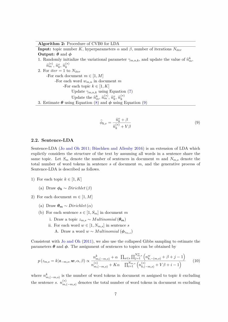
2.2. Sentence-LDA
Sentence-LDA (Jo and Oh 2011; Büschken and Allenby 2016) is an extension of LDA whichexplictly considers the structure of the text by assuming all words in a sentence share thesame topic. Let Sm denote the number of sentences in document m and Nm,s denote thetotal number of word tokens in sentence s of document m, and the generative process ofSentence-LDA is described as follows.
1) For each topic k ∈ [1,K]
(a) Draw φk ∼ Dirichlet (β)
2) For each document m ∈ [1,M ]
(a) Draw θm ∼ Dirichlet (α)(b) For each sentence s ∈ [1, Sm] in document m
i. Draw a topic zm,s ∼Multinomial (θm)ii. For each word w ∈ [1, Nm,s] in sentence s
A. Draw a word w ∼Multinomial(φzm,s
)Consistent with Jo and Oh (2011), we also use the collapsed Gibbs sampling to estimate theparameters θ and φ. The assignment of sentences to topics can be obtained by
p (zm,s = k|z−m,s,w, α, β) ∝nkm,(−m,s) + α
n(∗)m,(−m,s) +Kα
∏w∈s
∏Nwm,s
j=1
(nwk,−(m,s) + β + j − 1
)∏Nm,s
i=1
(n
(∗)k,(−m,s) + V β + i− 1
) (10)
where nkm,(−m,s) is the number of word tokens in document m assigned to topic k excludingthe sentence s. n(∗)
m,(−m,s) denotes the total number of word tokens in document m excluding
7

Algorithm 3: Procedure of collapsed Gibbs sampling for Sentence-LDAInput: topic number K, hyperparameters α and β, number of iterations Niter
Output: θ and φ1. Randomly initialize the topic assignment zm,s for each sentence, and update the count nkm,
n(∗)m , nvk, n
(∗)k
2. For iter = 1 to Niter
-For each document m ∈ [1,M ]-For each sentence s ∈ [1, Sm] in document m
Sample the topic k using Equation (10)Update the nkm, n
(∗)m , nvk, n
(∗)k
3. Estimate θ using Equation (11) and φ using Equation (12)
the sentence s. Nwm,s denotes the number of occurrences of word w in the sentence s. nwk,−(m,s)
is the number of tokens of word w assigned to topic k excluding the sentence s. n(∗)k,(−m,s)
denotes the total number of word tokens assigned to topic k excluding the sentence s.We present the procedure of collapsed Gibbs sampling for Sentence-LDA in Algorithm 3.Specifically, the parameters θ and φ are given by Equation (11) and Equation (12).
θm,k = nkm + α
n(∗)m +Kα
(11)
φk,v = nvk + β
n(∗)k + V β
(12)
2.3. HDPHDP (hierarchical Dirichlet process) (Teh et al. 2005) is a nonparametric Bayesian model onthe basis of the Dirichlet process. LDA uses Dirichlet distribution to characterize the shadesof membership to different topics, and assumes that the number of topics is fixed and finite.However, HDP assumes that there is an infinite number of topics, and allows the model todetermine an optimal number of topics automatically.The Dirichlet process DP (γ,H) is in essence a measure on measures. It can be describedby two parameters: a scaling (or concentration) parameter γ > 0 and a base measure H.To provide an explicit way to construct a Dirichlet process, Sethuraman (1994) proposes thestick-breaking process. Specifically, a sample G0 drawn from DP (γ,H) can be defined as:
G0 =∞∑k=1
πkδφk(13)
where δφkis a probability measure concentrated at φk which are independent and identically
distributed draws from the base measure H. Parameters π = {πk}∞k=1 denote a set of weightsand satisfy
∑∞k=1 πk = 1. Each πk is defined on the basis of independent and identically
distributed draws from Beta(1, γ):
πk = πk′k−1∏l=1
(1− πl′
)πk′|γ ∼ Beta (1, γ)
(14)
8

For convenience and clarity, the above two steps in Equation (14) are commonly written asπ ∼ GEM(γ) where GEM refers to Griffiths, Engen and McCloskey (Teh et al. 2005).According to Teh et al. (2005), HDP can be constructed via two-level stick-breaking repre-sentations. Particularly, in corpus level, the global measure G0 follows the standard Dirichletprocess, which is expressed as:
G0 =∞∑k=1
πkδφk
φk|H ∼ Hπ|γ = {πk}∞k=1 ∼ GEM (γ)
(15)
In document level, the random measure Gm also follows standard Dirichlet process where thebase measure is G0. The details is given by:
Gm =∞∑k=1
θm,kδφk
θm,k = θ′m,k
k−1∏l=1
(1− θ′m,l
)
θ′m,k|α0,π ∼ Beta
(α0πk, α0
(1−
k∑l=1
πl
)) (16)
HDP contains two additional steps for modeling the documents. First, it chooses a topic zm,nrelated to the word wm,n, and then generates the word from φzm,n . The details are shown inEquation (17).
zm,n|θm ∼Multinomial (θm)wm,n|zm,n, {φk}∞k=1 ∼Multinomial
(φzm,n
) (17)
For HDP, Teh et al. (2005) use Gibbs sampling on the basis of Chinese restaurant franchiseto infer the topic assignment zm,n. We first calculate the conditional density f−m,nk of wm,nunder topic k given all data items except wm,n:
f−m,nk (wm,n = v) =
∫p (wm,n|φk)
∏m′ ,n′ 6=m,n;z
m′,n′=k p
(wm′ ,n′ |φk
)p (φk|β) dφk∫ ∏
m′ ,n′ 6=m,n;zm′,n′=k p
(wm′ ,n′ |φk
)p (φk|β) dφk
=
nv
k+βn
(∗)k
+V β, if k exists
1V if k is new
(18)
Based on the idea Chinese restaurant franchise, we next calculate the probability of assigninga table t to word wm,n:
p (tm,n = t|t−m,n,k) ∝
n−m,nm,t,∗ f−m,nkm,t
(wm,n) if t previously used
α0p (wm,n|t−m,n, tm,n = tnew,k) if t = tnew(19)
9

Algorithm 4: Procedure of HDP learningInput: initial topic number K, hyperparameters α0, β and γ, number of iterations Niter
Output: θ and φ1. Randomly initialize the table assignments tm,n for each word, topic assignment kmtnew for
each new table, and update the count nm,t,∗, nvk, n(∗)k , m∗k and m∗∗
2. For iter = 1 to Niter
-For each document m ∈ [1,M ]-For each word wm,n in document m
-Ensure the capacity so that new table and new topic can be chosen-Sample the table t using Equation (19)-If t = tnew
Sample the topic for this table using Equation (21)-Update the count nm,t,∗, nvk, n
(∗)k , m∗k and m∗∗
- Remove the empty topic and table, and then re-arrange topic and table indices3. Estimate θ using Equation (22) and φ using Equation (23)
where n−m,nm,t,∗ denotes the number of words in document m that assign to table t, leaving outword wm,n. Let p (wm,n|t−m,n, tm,n = tnew,k) denote the likelihood for tm,n = tnew, which iscalculated as
p (wm,n|t−m,n, tm,n = tnew,k) =K∑k=1
m∗km∗∗ + γ
f−m,nk (wm,n) + γ
m∗∗ + γf−m,nk=knew (wm,n) (20)
where m∗k is the number of tables that belong to topic k. m∗∗ is the total number of tables.If tm,n equals tnew, we sample a new topic kmtnew for the new table tnew:
p(kmtnew = k|t,k−mtnew
)∝{m∗kf
−m,nk (ww,n) if k exists
γf−m,nknew (wm,n) if k = knew(21)
We present the procedure of HDP learning in Algorithm 4. According to the topic assignmentsfor each table, we compute nkm by counting tokens in document m assigned to topic k andn
(∗)m by counting tokens in document m. Then, we estimate θ and φ by Equation (22) and
(23)
θm,k = nkm + α0
n(∗)m +Kα0
(22)
φk,v = nvk + β
n(∗)k + V β
(23)
2.4. DMM
Short text clustering is an important task for NLP. Dirichlet Multinomial Mixture (DMM)model used in Nigam et al. (2000) is a popular generative model for short text clustering. Thisapproach contains two assumptions: (1) each short document is generated from a cluster, and(2) each cluster is a multinomial distribution over words. The generative process of DMM isdescribed as follows.
10
1) For each cluster k ∈ [1,K]
(a) Draw φk ∼ Dirichlet (β)
2) Draw the global cluster distribution θ ∼ Dirichlet (α)
3) For each document m ∈ [1,M ]
(a) Draw the cluster zm ∼Multinomial (θ)(b) For each word wm,n in document m
i. Draw wm,n ∼Multinomial (φzm)
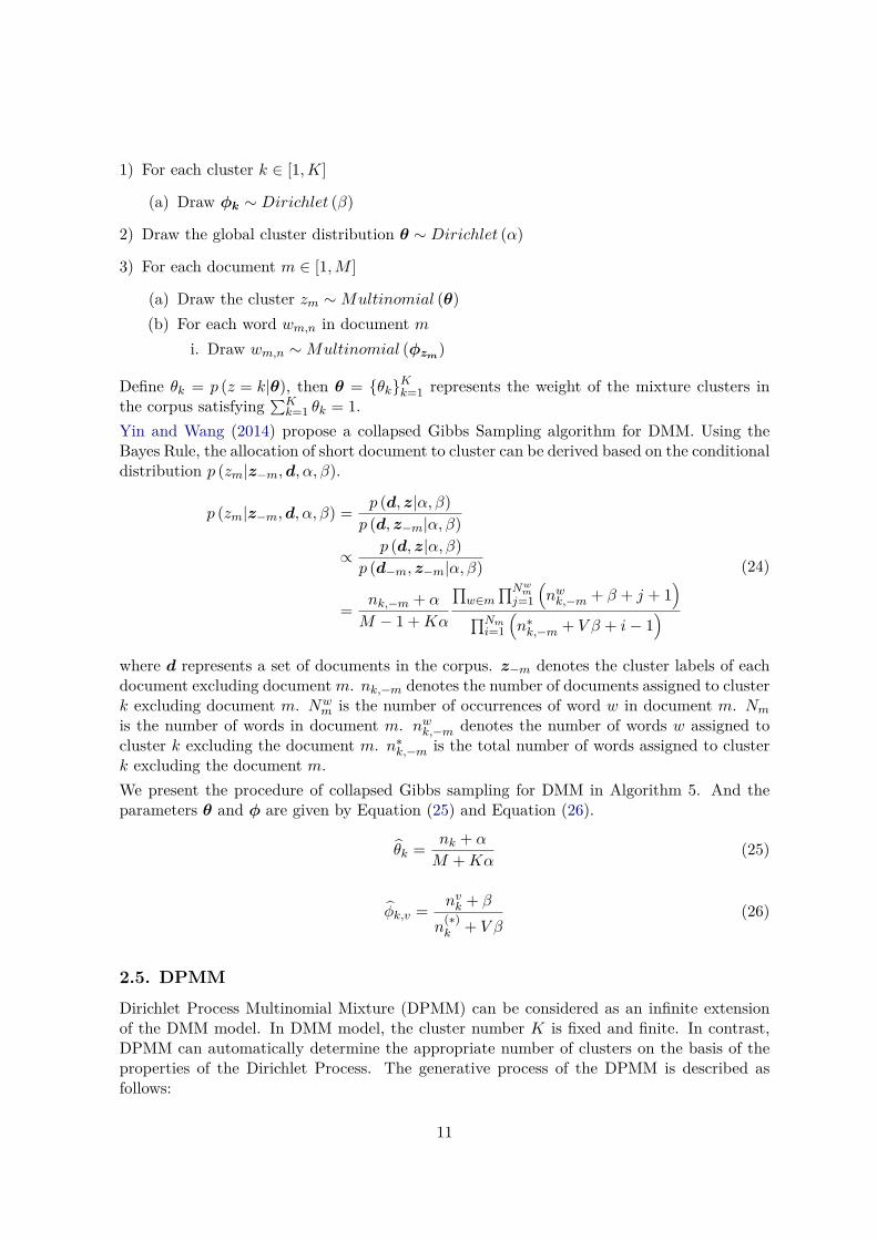
Define θk = p (z = k|θ), then θ = {θk}Kk=1 represents the weight of the mixture clusters inthe corpus satisfying
∑Kk=1 θk = 1.
Yin and Wang (2014) propose a collapsed Gibbs Sampling algorithm for DMM. Using theBayes Rule, the allocation of short document to cluster can be derived based on the conditionaldistribution p (zm|z−m,d, α, β).
p (zm|z−m,d, α, β) = p (d, z|α, β)p (d, z−m|α, β)
∝ p (d, z|α, β)p (d−m, z−m|α, β)
= nk,−m + α
M − 1 +Kα
∏w∈m
∏Nwm
j=1
(nwk,−m + β + j + 1
)∏Nmi=1
(n∗k,−m + V β + i− 1
)(24)
where d represents a set of documents in the corpus. z−m denotes the cluster labels of eachdocument excluding documentm. nk,−m denotes the number of documents assigned to clusterk excluding document m. Nw
m is the number of occurrences of word w in document m. Nm
is the number of words in document m. nwk,−m denotes the number of words w assigned tocluster k excluding the document m. n∗k,−m is the total number of words assigned to clusterk excluding the document m.We present the procedure of collapsed Gibbs sampling for DMM in Algorithm 5. And theparameters θ and φ are given by Equation (25) and Equation (26).
θk = nk + α
M +Kα(25)
φk,v = nvk + β
n(∗)k + V β
(26)
2.5. DPMM
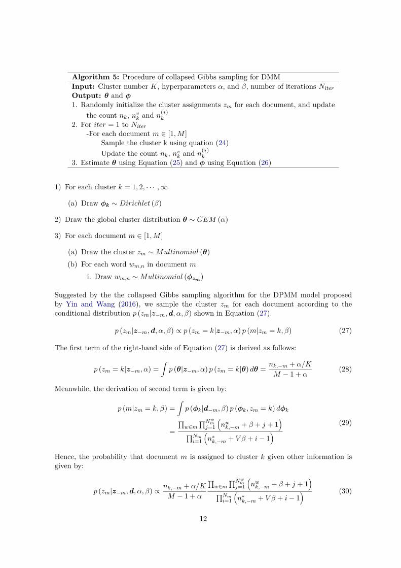
Dirichlet Process Multinomial Mixture (DPMM) can be considered as an infinite extensionof the DMM model. In DMM model, the cluster number K is fixed and finite. In contrast,DPMM can automatically determine the appropriate number of clusters on the basis of theproperties of the Dirichlet Process. The generative process of the DPMM is described asfollows:
11
Algorithm 5: Procedure of collapsed Gibbs sampling for DMMInput: Cluster number K, hyperparameters α, and β, number of iterations Niter
Output: θ and φ1. Randomly initialize the cluster assignments zm for each document, and update
the count nk, nvk and n(∗)k
2. For iter = 1 to Niter
-For each document m ∈ [1,M ]Sample the cluster k using quation (24)Update the count nk, nvk and n(∗)
k
3. Estimate θ using Equation (25) and φ using Equation (26)
1) For each cluster k = 1, 2, · · · ,∞
(a) Draw φk ∼ Dirichlet (β)
2) Draw the global cluster distribution θ ∼ GEM (α)
3) For each document m ∈ [1,M ]
(a) Draw the cluster zm ∼Multinomial (θ)(b) For each word wm,n in document m
i. Draw wm,n ∼Multinomial (φzm)
Suggested by the the collapsed Gibbs sampling algorithm for the DPMM model proposedby Yin and Wang (2016), we sample the cluster zm for each document according to theconditional distribution p (zm|z−m,d, α, β) shown in Equation (27).
p (zm|z−m,d, α, β) ∝ p (zm = k|z−m, α) p (m|zm = k, β) (27)
The first term of the right-hand side of Equation (27) is derived as follows:
p (zm = k|z−m, α) =∫p (θ|z−m, α) p (zm = k|θ) dθ = nk,−m + α/K
M − 1 + α(28)
Meanwhile, the derivation of second term is given by:
p (m|zm = k, β) =∫p (φk|d−m, β) p (φk, zm = k) dφk
=∏w∈m
∏Nwm
j=1
(nwk,−m + β + j + 1
)∏Nmi=1
(n∗k,−m + V β + i− 1
) (29)
Hence, the probability that document m is assigned to cluster k given other information isgiven by:
p (zm|z−m,d, α, β) ∝ nk,−m + α/K
M − 1 + α
∏w∈m
∏Nwm
j=1
(nwk,−m + β + j + 1
)∏Nmi=1
(n∗k,−m + V β + i− 1
) (30)
12

Let K go to infinity (∞), we can obtain the probability of document m assigned to an existingcluster k as follows:
p (zm|z−m,d, α, β) ∝ nk,−mM − 1 + α
∏w∈m
∏Nwm
j=1
(nwk,−m + β + j + 1
)∏Nmi=1
(n∗k,−m + V β + i− 1
) (31)
Denoting a new cluster as knew, we obtain the probability of document m being assigned tocluster knew as:
p (zm|z−m,d, α, β) ∝ α
M − 1 + α
∏w∈m
∏Nwm
j=1 (β + j + 1)∏Nmi=1 (V β + i− 1)
(32)
Finally, we combine Equation (31) and Equation (32), and obtain:
p (zm|z−m,d, α, β) ∝
nk,−mM − 1 + α
∏w∈m
∏Nwm
j=1
(nwk,−m + β + j + 1
)∏Nmi=1
(n∗k,−m + V β + i− 1
) if k exists
α
M − 1 + α
∏w∈m
∏Nwm
j=1 (β + j + 1)∏Nmi=1 (V β + i− 1)
if k = knew
(33)
We present the procedure of collapsed Gibbs sampling for DPMM in Algorithm 6. Similar toDMM, we can estimate the parameters θ and φ by Equation (34) and Equation (35).
θk = nk + α
M +Kα(34)
φk,v = nvk + β
n(∗)k + V β
(35)
2.6. PTM
Due to the sparsity of word co-occurrences in short documents, LDA struggles to obtain sat-isfactory performances. To solve this problem, Pseudo-document-based Topic Model (PTM)is proposed by Zuo et al. (2016) where pseudo documents are introduced for indirect aggre-gation of short texts. In PTM, a large of short documents is transformed into relatively fewpseudo documents (long text) to avoid data sparsity, which could improve the topic learning.We assume that there are P pseudo documents and each one is denoted as l ∈ [1, P ]. Letψ denote a multinomial distribution which models the distribution of short documents overpseudo documents. In PTM, each short document is assigned to one pseudo document. Forgenerating each word in a short document, PTM first sample a topic z from topic distributionθ over pseudo document, and then sample a word from the topic-word distribution φz. Thegenerative process of the PTM is described as follows:
1) Draw ϕ ∼ Dirichlet (λ)
2) For each topic k ∈ [1,K]
(a) Draw φk ∼ Dirichlet (β)
13

Algorithm 6: Procedure of collapsed Gibbs sampling for DPMMInput: initial cluster number K, hyperparameters α, and β, number of iterations Niter
Output: θ and φ1. Randomly initialize the cluster assignments zm for each document, and update
the count nk, nvk and n(∗)k
2. For iter = 1 to Niter
-For each document m ∈ [1,M ]-Record the current cluster of m as k, and update the count nk,−m, nwk,−m and n(∗)
k,−m-If nk = 0
//Remove the inactive clusterK = K − 1Re-arrange cluster indices
-Sample the cluster k using Equation (33)-If k = knew
//A new clusterK = K + 1Initialize the count nk, nvk and n(∗)
k as zero-Update the count nk, nvk and n(∗)
k
3. Estimate θ using Equation (34) and φ using Equation (35)
3) For each pseudo document l ∈ [1, P ]
(a) Draw θl ∼ Dirichlet (α)
4) For each short document m ∈ [1,M ]
(a) Draw a pseudo document lm ∼Multinomial (ϕ)(b) For each word wm,n in document m
i. Draw the topic zm,n ∼Multinomial (θlm)ii. Draw wm,n ∼Multinomial
(φzm,n
)Same as Zuo et al. (2016), we use the collapsed Gibbs sampling algorithm for model estima-tion. In PTM, there are two latent variables needed to iterate by the sampling algorithm:pseudo document assignment l and topic assignment z. Conditioned on all the other doc-uments, the probability of a short document lm being assigned to a pseudo document l iswritten as:
p (lm = l|rest) ∝ nl,−m + λ
M − 1 + Pλ
∏k∈m
∏Nkm
j=1
(Nkl,−m + α+ j − 1
)∏Nmi=1
(N
(∗)l,−m +Kα+ i− 1
) (36)
where nl,−m is the number of short documents assigned to the pseudo document l excludingdocument m. Nk
m is the number of words assigned to topic k in document m. Nkl,−m denotes
the number of words assigned to topic k in pseudo document l excluding document m. N (∗)l,−m
denotes is the total number of words in pseudo document l excluding document m. Nm isthe number of words in document m.
14

Algorithm 7: Procedure of collapsed Gibbs sampling for PTMInput: topic number K, number of pseudo document P , hyperparameters α, β and γ,
number of iterations Niter
Output: θ and φ1. Randomly initialize the pseudo document assignment lm for each document;
randomly initialize the topic assignments z(m,n) for each word;update the count nl, Nk
l , N(∗)l ,nvk and n(
k(∗))2. For iter = 1 to Niter
-For each document m ∈ [1,M ]Sample the pseudo document assignment l using Equation (36)Update the count nl, Nk
l and N (∗)l
-For each document m ∈ [1,M ]-For each word wm,n in document m
Sample the topic k using Equation (37)Update the count Nk
l , N(∗)l , nvk and n(∗)
k
3. Estimate θ using Equation (38) and φ using Equation (39)
We can sample the topic zm,n for each word according to the conditional probability ofzm,n = k, which is given by:
p (zm,n = k|wm,n = v, rest) ∝Nkl,(−m,n) + α
N∗l,(−m,n) +Kα
nvk,(−m,n) + β
n(∗)k,(−m,n) + V β
(37)
Algorithm 7 shows the procedure of collapsed Gibbs sampling for PTM. Note that PTM learnthe topic distribution θl for each pseudo document l. However, we can count nkm and n
(∗)m
according to topic assignment zm,n. Then we obtain topic distribution θm for each shortdocument as follows:
θm,k = nkm + α
n(∗)m +Kα
(38)
From Equation (39), we can estimate the parameter φ.
φk,v = nvk + β
n(∗)k + V β
(39)
2.7. BTM
To cope with the sparsity of word co-occurrence patterns in short text, BTM is proposed byCheng et al. (2014); Yan et al. (2013). Unlike LDA and DMM, BTM assumes that a bitermis an unordered word-pair generated from a short text, and the two words in the biterm sharethe same topic. In addition, each topic for the biterm is drawn from a global topic distributionover the corpus.In BTM, the first step is to construct biterms on the basis of short texts and a fixed-sizewindow. For example, we can construct three biterms from a document with three distinctwords:
(w1, w2, w2)→ (w1, w2), (w2, w3), (w1, w3) (40)
15
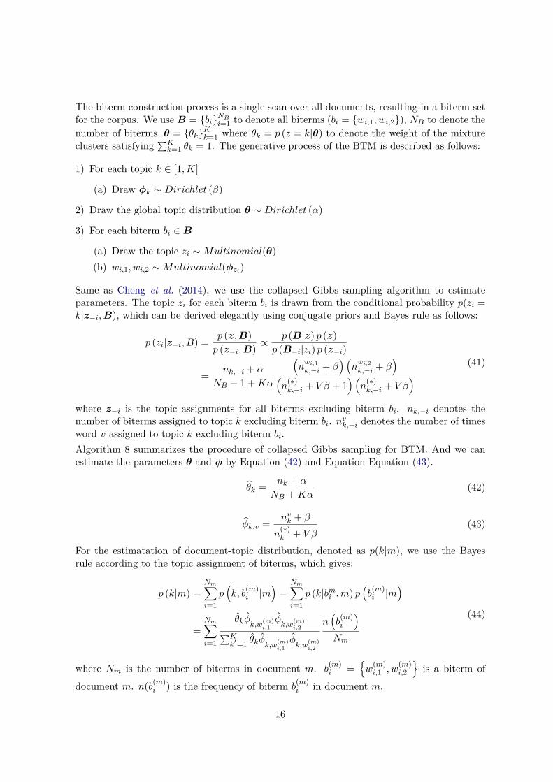
The biterm construction process is a single scan over all documents, resulting in a biterm setfor the corpus. We use B = {bi}NB
i=1 to denote all biterms (bi = {wi,1, wi,2}), NB to denote thenumber of biterms, θ = {θk}Kk=1 where θk = p (z = k|θ) to denote the weight of the mixtureclusters satisfying
∑Kk=1 θk = 1. The generative process of the BTM is described as follows:
1) For each topic k ∈ [1,K]
(a) Draw φk ∼ Dirichlet (β)
2) Draw the global topic distribution θ ∼ Dirichlet (α)
3) For each biterm bi ∈ B
(a) Draw the topic zi ∼Multinomial(θ)(b) wi,1, wi,2 ∼Multinomial(φzi)
Same as Cheng et al. (2014), we use the collapsed Gibbs sampling algorithm to estimateparameters. The topic zi for each biterm bi is drawn from the conditional probability p(zi =k|z−i,B), which can be derived elegantly using conjugate priors and Bayes rule as follows:
p (zi|z−i, B) = p (z,B)p (z−i,B) ∝
p (B|z) p (z)p (B−i|zi) p (z−i)
= nk,−i + α
NB − 1 +Kα
(nwi,1k,−i + β
) (nwi,2k,−i + β
)(n
(∗)k,−i + V β + 1
) (n
(∗)k,−i + V β
) (41)
where z−i is the topic assignments for all biterms excluding biterm bi. nk,−i denotes thenumber of biterms assigned to topic k excluding biterm bi. nvk,−i denotes the number of timesword v assigned to topic k excluding biterm bi.Algorithm 8 summarizes the procedure of collapsed Gibbs sampling for BTM. And we canestimate the parameters θ and φ by Equation (42) and Equation Equation (43).
θk = nk + α
NB +Kα(42)
φk,v = nvk + β
n(∗)k + V β
(43)
For the estimatation of document-topic distribution, denoted as p(k|m), we use the Bayesrule according to the topic assignment of biterms, which gives:
p (k|m) =Nm∑i=1
p(k, b
(m)i |m
)=
Nm∑i=1
p (k|bmi ,m) p(b
(m)i |m
)
=Nm∑i=1
θkφk,w(m)i,1φk,w
(m)i,2∑K
k′=1 θkφk,w(m)i,1φk,w
(m)i,2
n(b
(m)i
)Nm
(44)
where Nm is the number of biterms in document m. b(m)i =
{w
(m)i,1 , w
(m)i,2
}is a biterm of
document m. n(b(m)i ) is the frequency of biterm b
(m)i in document m.
16

Algorithm 8: Procedure of collapsed Gibbs sampling for BTMInput: topic number K, hyperparameters α and β, number of iterations Niter
Output: θ, φ and p(k|m)1. Construct biterms on the basis of short texts and a fixed-size window2. Randomly initialize the topic assignment zi for each biterm, and update the count nk, nvk , n(∗)
k
3. For iter = 1 to Niter
-For each biterm bi ∈ BSample the topic k using Equation (41)Update the count nk, nvk , n(∗)
k
4. Estimate θ using Equation (42) and φ using Equation (43)5. Estimate p(k|m) using Equation (44)
2.8. ATM
To capture authorship information, a critical aspect for documents such as academic publi-cations, Author-topic model (ATM) (Rosen-Zvi et al. 2004) is proposed with the underlyingassuption that each author is related to a multinomial distribution over topics while eachtopic is characterised by a multinomial distribution over words. For documents with multipleauthors, the distribution over topics is an admixture of the distributions corresponding to theauthors. In this way, ATM can discover salient latent topics as well as interesting patternsfor each author.In ATM, a document is generated via the following process. First, an author is randomly se-lected for each word. Second, a topic is chosen from the author-topic multinomial distributionassociated with the selected author. Finally, a word is drawn from the topic-word multinomialdistribution conditioned on the chosen topic. Let am denote the authors of document m andxm,n denote the author assignment for the word wm,n. The generative process is detailed asfollows:
1) For each author a ∈ [1, A]
(a) Draw θa ∼ Dirichlet (α)
2) For each topic k ∈ [1,K]
(a) Draw φk ∼ Dirichlet (β)
3) For each document m ∈ [1,M ]
(a) Given the authors am of document m(b) For each word wm,n in document m
i. Draw an author xm,n ∼ Uniform(am)ii. Draw the topic zm,n ∼Multinomial(θxm,n)iii. Draw the word wm,n ∼Multinomial(φzm,n)
Same as Rosen-Zvi et al. (2004), we apply the collapsed Gibbs sampling algorithm to es-timate the parameters. For each word wm,n, the associated author and topic are sampled
17
Algorithm 9: Procedure of collapsed Gibbs sampling for ATMInput: topic number K, hyperparameters α and β, number of iterations Niter
Output: θ, φ1. Randomly initialize the topic assignment zm,n and the author assignment a for each word;
update the count nka, n(∗)a , nvk, n
(∗)k
2. For iter = 1 to Niter
-For each document m ∈ [1,M ]-For each word wm,n in document m
Sample the topic k and the author a using Equation (45)Update the count nka, n
(∗)a , nvk, n
(∗)k
3. Estimate θ using Equation (46) and φ using Equation (47)
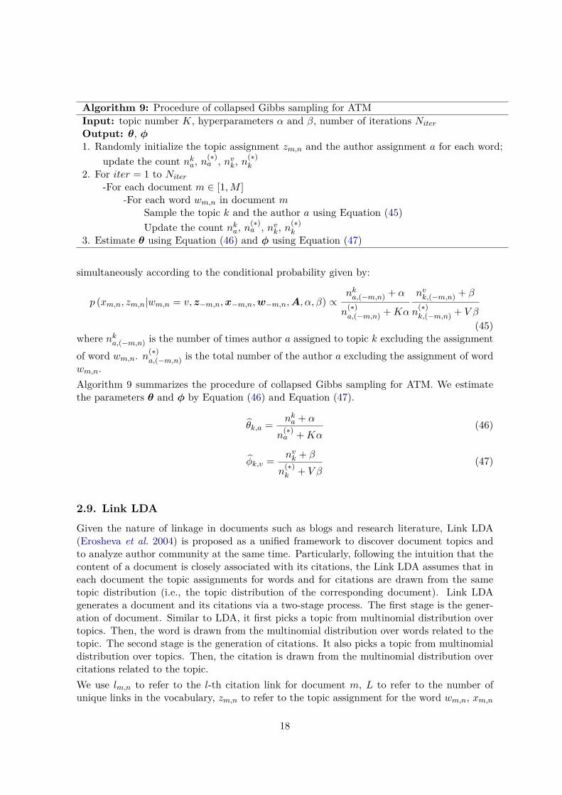
simultaneously according to the conditional probability given by:
p (xm,n, zm,n|wm,n = v, z−m,n,x−m,n,w−m,n,A, α, β) ∝nka,(−m,n) + α
n(∗)a,(−m,n) +Kα
nvk,(−m,n) + β
n(∗)k,(−m,n) + V β
(45)where nka,(−m,n) is the number of times author a assigned to topic k excluding the assignmentof word wm,n. n(∗)
a,(−m,n) is the total number of the author a excluding the assignment of wordwm,n.Algorithm 9 summarizes the procedure of collapsed Gibbs sampling for ATM. We estimatethe parameters θ and φ by Equation (46) and Equation (47).
θk,a = nka + α
n(∗)a +Kα
(46)
φk,v = nvk + β
n(∗)k + V β
(47)
2.9. Link LDA
Given the nature of linkage in documents such as blogs and research literature, Link LDA(Erosheva et al. 2004) is proposed as a unified framework to discover document topics andto analyze author community at the same time. Particularly, following the intuition that thecontent of a document is closely associated with its citations, the Link LDA assumes that ineach document the topic assignments for words and for citations are drawn from the sametopic distribution (i.e., the topic distribution of the corresponding document). Link LDAgenerates a document and its citations via a two-stage process. The first stage is the gener-ation of document. Similar to LDA, it first picks a topic from multinomial distribution overtopics. Then, the word is drawn from the multinomial distribution over words related to thetopic. The second stage is the generation of citations. It also picks a topic from multinomialdistribution over topics. Then, the citation is drawn from the multinomial distribution overcitations related to the topic.We use lm,n to refer to the l-th citation link for document m, L to refer to the number ofunique links in the vocabulary, zm,n to refer to the topic assignment for the word wm,n, xm,n
18

to refer to the topic assignment for the link lm,n, and ϕ to refer to per-topic link distribution.The generative process of the Link LDA is described as follows:
1) For each topic k ∈ [1,K]
(a) Draw topic-word distribution φk ∼ Dirichlet (β)(b) Draw topic-link distribution ϕk ∼ Dirichlet (γ)
2) For each document m ∈ [1,M ]
(a) Draw θm ∼ Dirichlet (α)(b) For each word wm,n in document m
i. Draw the topic zm,n ∼Multinomial(θm)ii. Draw the word wm,n ∼Multinomial(φzm,n)
(c) For each link lm,n for document mi. Draw the topic xm,n ∼Multinomial(θm)ii. Draw the link lm,n ∼Multinomial(ϕxm,n)
Same as the orginal paper (Erosheva et al. 2004), in estimation, we utilize the collapsed Gibbssampling where latent variables z and x are sampled iteratively. Specifically, we first samplethe topic assignments zm,n for the word wm,n according to the posterior distribution:
p(zm,n = k|wm,n = v, z−m,n,w−m,n,x, α, β) ∝nvk,(−m,n) + β
n(∗)k,(−m,n) + V β
(nkm,(−m,n) + ckm + α
)(48)
Next, we sample the topic assignments xm,e for the link on the basis of posterior distribution:p(xm,e = k|lm,e = l,x−m,e, l−m,e, z, α, γ):
p(xm,e = k|lm,e = l,x−m,e, l−m,e, z, α, γ) ∝clk,(−m,e) + γ
c(∗)k,(−m,e) + Lγ
(ckm,(−m,e) + nkm + α
)(49)
where nvk is the number of times word v assigned to topic k. n(∗)k denotes the total number of
words assigned to topic k. nkm is the number of words in document m assigned to topic k. ckmis the number of links for document m assigned to topic k. clk is the number of times link lassigned to topic k. c(∗)
k is the total number of links assigned to topic k. The notation −m,nrefers to the corresponding count excluding the current assignment of the word wm,n. Thenotation −m, e refers to the corresponding count excluding the current assignment of the linklm,e.Algorithm 10 summarizes the procedure of collapsed Gibbs sampling for Link LDA. After thesampling algorithm has achieved convergece with appropriate iterations, we can estimate theparameters θ, φ and ϕ via the following equations:
θm,k = nkm + ckm + α∑Kk′=1
(nk′m + ck
′m
)+Kα
(50)
φk,v = nvk + β
n(∗)k + V β
(51)
19

Algorithm 10: Procedure of collapsed Gibbs sampling for link LDAInput: topic number K, hyperparameters α, β and γ, number of iterations Niter
Output: θ, φ and ϕ1. Randomly initialize the topic assignment zm,n for each word and the topic assignment xm,e
for each link; update the count nkm, ckm, nvk, n(∗)k , clk, c
(∗)k
2. For iter = 1 to Niter
-For each document m ∈ [1,M ]-For each word wm,n in document m
Sample the topic k using Equation (48)Update the count nkm, nvk, n
(∗)k
-For each link lm,e for document mSample the topic k using Equation (49)Update the count ckm, clk, c
(∗)k
3. Estimate θ using Equation (50), φ using Equation (51) and ϕ using Equation (52)
ϕk,l = clk + γ
c(∗)k + Lγ
(52)
2.10. Labeled LDA
To incorporate supervision information, Labeled LDA (Ramage et al. 2009) is proposed as su-pervised topic model for documents with multiple labels. It learns word-label correspondencesdirectly by introducing a one-to-one correspondence between latent topics and document la-bels. Besides, the topics of each document are restricted to be defined only over the documentlabel sets. The extension allows the Labeled LDA gain advantages over standard LDA suchas the ability to assign a document’s words to its labels as well as enhanced interpretabilityof topics.For Labeled LDA, let Λm = {l1, l2, · · · , lK} denote a list of binary topic absence indicatorsfor document m, where each lk ∈ {0, 1}. The number of topics is equal to the number ofunique labels K in the corpus. Ψk is the label prior for topic k. λm =
{k|Λkm = 1
}denotes
the vector of labels of document m, where Λkm ∈ Λm. L(m) represents a document-specificlabel projection matrix with the size of Pm×K, where Pm =
∣∣∣λ(m)∣∣∣. For each row i ∈ [1, Pm]
and column k ∈ [1,K], L(m) can be defined as follows:
L(m)ik =
{1 if λ
(m)i = k
0 otherwise(53)
To restrict the topic of document m to its own labels, Labeled LDA introduces a lowerdimensional vector α(m) = L(m) ×α where α = (α1, α2, · · · , αK) is the Dirichlet topic prior.The generative process of the Labeled LDA is described as follows:
1) For each topic k ∈ [1,K]
(a) Draw topic-word distribution φk ∼ Dirichlet (β)
20
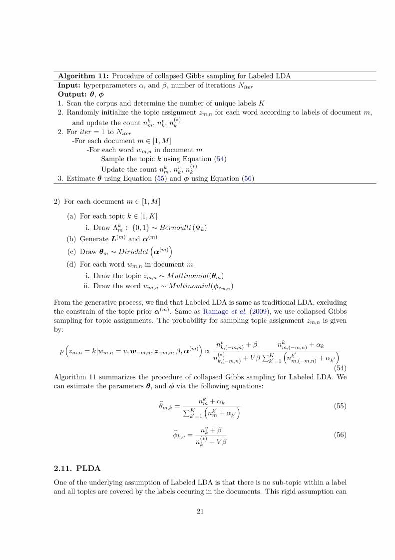
Algorithm 11: Procedure of collapsed Gibbs sampling for Labeled LDAInput: hyperparameters α, and β, number of iterations Niter
Output: θ, φ1. Scan the corpus and determine the number of unique labels K2. Randomly initialize the topic assignment zm,n for each word according to labels of document m,
and update the count nkm, nvk, n(∗)k
2. For iter = 1 to Niter
-For each document m ∈ [1,M ]-For each word wm,n in document m
Sample the topic k using Equation (54)Update the count nkm, nvk, n
(∗)k
3. Estimate θ using Equation (55) and φ using Equation (56)
2) For each document m ∈ [1,M ]
(a) For each topic k ∈ [1,K]i. Draw Λkm ∈ {0, 1} ∼ Bernoulli (Ψk)
(b) Generate L(m) and α(m)
(c) Draw θm ∼ Dirichlet(α(m)
)(d) For each word wm,n in document m
i. Draw the topic zm,n ∼Multinomial(θm)ii. Draw the word wm,n ∼Multinomial(φzm,n)
From the generative process, we find that Labeled LDA is same as traditional LDA, excludingthe constrain of the topic prior α(m). Same as Ramage et al. (2009), we use collapsed Gibbssampling for topic assignments. The probability for sampling topic assignment zm,n is givenby:
p(zm,n = k|wm,n = v,w−m,n, z−m,n, β,α
(m))∝
nvk,(−m,n) + β
n(∗)k,(−m,n) + V β
nkm,(−m,n) + αk∑Kk′=1
(nk′
m,(−m,n) + αk′)(54)
Algorithm 11 summarizes the procedure of collapsed Gibbs sampling for Labeled LDA. Wecan estimate the parameters θ, and φ via the following equations:
θm,k = nkm + αk∑Kk′=1
(nk′m + αk′
) (55)
φk,v = nvk + β
n(∗)k + V β
(56)
2.11. PLDA
One of the underlying assumption of Labeled LDA is that there is no sub-topic within a labeland all topics are covered by the labels occuring in the documents. This rigid assumption can
21
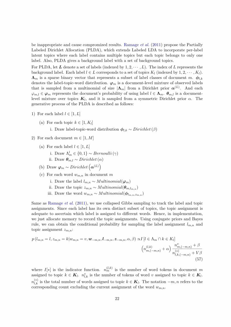
be inappropriate and cause compromized results. Ramage et al. (2011) propose the PartiallyLabeled Dirichlet Allocation (PLDA), which extends Labeled LDA to incorporate per-labellatent topics where each label contains multiple topics but each topic belongs to only onelabel. Also, PLDA gives a background label with a set of background topics.For PLDA, let L denote a set of labels (indexed by 1, 2, · · · , L). The index of L represents thebackground label. Each label l ∈ L corresponds to a set of topics Kl (indexed by 1, 2, · · · ,Kl).Λm is a sparse binary vector that represents a subset of label classes of document m. φl,kdenotes the label-topic-word distribution. ϕm is a document-level mixture of observed labelsthat is sampled from a multinomial of size |Λm| from a Dirichlet prior α(L). And eachϕm,l ∈ ϕm represents the document’s probability of using label l ∈ Λm. θm,l is a document-level mixture over topics Kl, and it is sampled from a symmetric Dirichlet prior α. Thegenerative process of the PLDA is described as follows:
1) For each label l ∈ [1, L]
(a) For each topic k ∈ [1,Kl]i. Draw label-topic-word distribution φl,k ∼ Dirichlet (β)
2) For each document m ∈ [1,M ]
(a) For each label l ∈ [1, L]i. Draw Λlm ∈ {0, 1} ∼ Bernoulli (γ)ii. Draw θm,l ∼ Dirichlet (α)
(b) Draw ϕm ∼ Dirichlet(α(L)
)(c) For each word wm,n in document m
i. Draw the label lm,n ∼Multinomial(ϕm)ii. Draw the topic zm,n ∼Multinomial(θm,lm,n)iii. Draw the word wm,n ∼Multinomial(φlm,n,zm,n)
Same as Ramage et al. (2011), we use collapsed Gibbs sampling to track the label and topicassignments. Since each label has its own distinct subset of topics, the topic assignment isadequate to ascertain which label is assigned to different words. Hence, in implementation,we just allocate memory to record the topic assignments. Using conjugate priors and Bayesrule, we can obtain the conditional probability for sampling the label assignment lm,n andtopic assignment zm,n:
p (lm,n = l, zm,n = k|wm,n = v,w−m,n, l−m,n, z−m,n, α, β) ∝I [l ∈ Λm ∩ k ∈ Kl](n
(l,k)m,(−m,n) + α
) nvm,(−m,n) + β
n(∗)l,k,(−m,n) + V β
(57)
where I[∗] is the indicator function. n(l,k)m is the number of word tokens in document m
assigned to topic k ∈ Kl. nvl,k is the number of tokens of word v assigned to topic k ∈ Kl.n
(∗)l,k is the total number of words assigned to topic k ∈Kl. The notation −m,n refers to the
corresponding count excluding the current assignment of the word wm,n.
22

Algorithm 12: Procedure of collapsed Gibbs sampling for PLDAInput: hyperparameters α and β,the topic number of Kl each label, number of iterations Niter
Output: θ, φ1. Scan the corpus and determine the number of unique labels L2. Allocate memory to represent each label l and its topics Kl
3. Randomly initialize the topic assignment zm,n for each word according to labels of document m,and update the count n(l,k,)
m , nvl,k, n(∗)l,k
4. For iter = 1 to Niter
-For each document m ∈ [1,M ]-For each word wm,n in document m
Sample the topic k using Equation (57)Update the count n(l,k,)
m , nvl,k, n(∗)l,k
5. Estimate θ using Equation (58) and φ using Equation (59)
Since each topic is related to only a single label, we can use empirical estimation to obtaindocument-topic proportion θm,k and topic-word proportion φk,v.
θm,k = nkm + αk∑Kk′=1
(nk′m + αk′
) (58)
φk,v = nvk + β
n(∗)k + V β
(59)
where K =∑Ll=1Kl is the total number of topics associated with labels. Algorithm 12
presents the procedure of collapsed Gibbs sampling for PLDA.
2.12. Dual-Sparse Topic ModelThe Dual-Sparse Topic Model is an effective approach for short documents modeling, whichis proposed by Lin et al. (2014). Classical topic models such as LDA usually utilize Dirichletprior to smooth the document-topic distributions and the topic-word distributions, thus failto control the posterior sparsity of the topic mixtures and the word distributions. In reality,a short document generally focuses on a small number of topics, and a topic is often charac-terized by a narrow range of words in the vocabulary. Thus, the topic mixtures and the worddistributions should have the feature of skewness or sparsity. In order to induce this sparsity,Dual-Sparse Topic Model introduces a "Spike and Slab" prior to decouple the sparsity andsmoothness of the document-topic distributions and topic-word distributions. This model iseasy enough to learn both a few focused topics for a document and focused words for a topic.For Dual-Sparse Topic Model, let αmk denote a topic selector that uses a binary variable toindicate whether a topic k is associated with document m. αmk is drawn from a Bernoullidistribution with a Bernoulli parameter am. βkv is a word selector that indicates whether theword v is involved in topic k. βkv is drawn from a Bernoulli distribution with a Bernoulliparameter bk. π and π are the topic smoothing prior and the weak topic smoothing prior,respectively. γ and γ are the word smoothing prior and the weak word smoothing prior,respectively. Since π << π and γ << γ, the model can easily induce the sparsity whilealso avoiding the ill-definition of the distributions. We describe the generative process of theDual-Sparse Topic Model as follows:
23
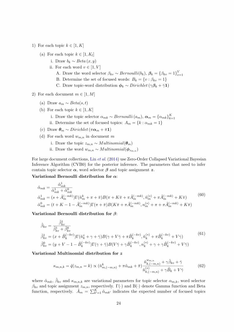
1) For each topic k ∈ [1,K]
(a) For each topic k ∈ [1,Kl]i. Draw bk ∼ Beta (x, y)ii. For each word v ∈ [1, V ]
A. Draw the word selector βkv ∼ Bernoulli(bk), βk = {βkv = 1}Vv=1B. Determine the set of focused words: Bk = {v : βkv = 1}C. Draw topic-word distribution φk ∼ Dirichlet (γβk + γ1)
2) For each document m ∈ [1,M ]
(a) Draw am ∼ Beta(s, t)(b) For each topic k ∈ [1,K]
i. Draw the topic selector αmk ∼ Bernoulli (am), αm = {αmk}Kk=1ii. Determine the set of focused topics: Am = {k : αmk = 1}
(c) Draw θm ∼ Dirichlet (παm + π1)(d) For each word wm,n in document m
i. Draw the topic zm,n ∼Multinomial(θm)ii. Draw the word wm,n ∼Multinomial(φzm,n)
For large document collections, Lin et al. (2014) use Zero-Order Collapsed Variational BayesianInference Algorithm (CVB0) for the posterior inference. The parameters that need to infercontain topic selector α, word selector β and topic assignment z.Variational Bernoulli distribution for α:
αmk = α1mk
α1mk + α0
mk
α1mk = (s+ A(−mk)
m )Γ(nkm + π + π)B(π +Kπ + πA(−mk)m , n(∗)
m + πA(−mk)m +Kπ)
α0mk = (t+K − 1− A(−mk)
m )Γ(π + π)B(Kπ + πA(−mk)m , n(∗)
m + π + πA(−mk)m +Kπ)
(60)
Variational Bernoulli distribution for β:
βkv = β1kv
β1kv + β0
kv
β1kv = (x+ B
(−kv)k )Γ(nvk + γ + γ)B(γ + V γ + πB
(−kv)k , n
(∗)k + πB
(−kv)k + V γ)
β0kv = (y + V − 1− B(−kv)
k )Γ(γ + γ)B(V γ + γB(−kv)k , n
(∗)k + γ + γB
(−kv)k + V γ)
(61)
Variational Multinomial distribution for z
κm,n,k = q(zm,n = k) ∝ (nkm,(−m,n) + παmk + π)nwm,n
k,(−m,n) + γβkv + γ
n(∗)k,(−m,n) + γBk + V γ
(62)
where αmk, βkv and κm,n,k are variational parameters for topic selector αm,k, word selectorβkv and topic assignment zm,n, respectively. Γ(·) and B(·) denote Gamma function and Betafunction, respectively. Am =
∑Kk′=1 αmk′ indicates the expected number of focused topics
24

for document m. nkm =∑n′ κm,n′,k denotes the expected number of word tokens assigned to
topic k in document m. n(∗)m =
∑n′,k′ κm,n′,k′ denotes the expected number of word tokens
in document m. Bm =∑Vv′=1 βkv indicates the expected number of focused words for topic
k. nvk =∑m′,n′ I
[wm′,n′ = v
]κm′,n′,k is the expected number of tokens of word v assigned
to topic k. n(∗)k =
∑m′,n′ κm′,n′,k is the expected number of words assigned to topic k. V
denotes the vocabulary size. The notation −mk, −kv, and −m,n mean αmk, βkv and wm,nare excluded, respectively.When the algorithm has reached convergence after an appropriate number of iterations, wecan estimate the parameters θ and φ via the following equations:
θm,k = nkm + παmk + π
n(∗)m + πAm +Kπ
(63)
φk,v = nvk + γβkv + γ
n(∗)k + πγBk + V γ
(64)
According to the estimated parameters α and β, we can measure the sparsity ratio of adocument-topic distribution and a topic-word distribution as follows:
sparsityD(m) = 1− AmK
(65)
sparsityT (k) = 1− BkV
(66)
The average sparsity ratio of all documents can be calculated as follows:
Asparsity − document = 1M
M∑m=1
sparsity(m) (67)
Asparsity − topic = 1K
K∑k=1
sparsity(k) (68)
Algorithm 13 shows the procedure of CVB0 for Dual-Sparse Topic Model.
3. The Use of TopicModel4J
3.1. Download Package
The TopicModel4J is implemented by the Java language. And it has been released under theGNU General Public License (GPL). All the source code for this package can be downloadedfrom https://github.com/soberqian/TopicModel4J. The researchers can run this packageon any platforms (e.g. Linux and Windows) that support Java 1.8. The dependencies for thispackage contain commons-math3 and Stanford CoreNLP(Manning, Surdeanu, Bauer, Finkel,Bethard, and McClosky 2014).
3.2. Data Pre-processing
25

Algorithm 13: Procedure of CVB0 for Dual-Sparse Topic ModelInput: hyperparameters x, y, γ, γ, s, t, π and π, K, number of iterations Niter
Output: θ, φ, sparsity(m), sparsity(k), Asparsity − document, Asparsity − topic1. Randomly initialize the variational parameter κm,n,k,
and update the value of nkm, n(∗)m , nvk and n(∗)
k
2. Randomly initialize αmk, βkv and update the value Am and Bk3. For iter = 1 to Niter
-For each document m ∈ [1,M ]- For each topic k ∈ [1,K]
Update αmk using Equation (60)Update Am
-For each topic k ∈ [1,K]-For each word v in vocabulary
Update βkv using Equation (61)-For each document m ∈ [1,M ]
-For each word wm,n in document m-For each topic k ∈ [1,K]
Update αmk, βkv using Equation Equation (62)4. Estimate θ using Equation (63), φ using Equation (64), sparsity(m) using Equation (65),
sparsity(k) using Equation (66), Asparsity − document using Equation (67), andAsparsity − topic using Equation (68)
For the tasks of NLP and text mining applications, the data pre-preprocessing is an importantprocedure before applying various machine learning models. It make the input data moreamenable for analysis and reliable discoveries. In TopicModel4J, we provide an easy-to-use interface for common text preprocessing techniques such as lowercasing, lemmatizationand stopword removal and noise removal. Next, we give two examples for the use of datapreprocessing in TopicModel4J. In the first example, we deal with a single document by thefollowing code:
String line = "http://t.cn/RAPgR4n Artificial intelligence is a known phenomenons "+ "in the world today. Its root started to build years";
//get all words for this documentArrayList<String> words = new ArrayList<String>();//lemmatizationFileUtil.getlema(line, words);//remove noise words using the default stop wordsString text = FileUtil.RemoveNoiseWord(words);//remove noise words using the customized stop wordsString text_c = FileUtil.RemoveNoiseWord(words,"data/stopwords");//print resultsSystem.out.println(text);System.out.println(text_c);
By the above code, we can remove uninformative words from the original document us-ing the default stop words defined by TopicModel4J. The default stop words contain 524
26

Figure 1: The content of the file "rawdataprocess"
common words (e.g., "a" and "the") that are given by BOW library (http://www.cs.cmu.edu/~mccallum/bow/). In order to meet the particular needs of researchers, TopicModel4Jalso provides an option to define a customized set of stop word list. For example, the"data/stopwords" in the above code is a file that includes many user-defined stop words(e.g. "year" and "today" ). Results after data preprocessing are shown below:
artificial intelligence phenomenon world today root start build yearartificial intelligence phenomenon world root start build
The second example is to show how mutiple documents are processed. In TopicModel4J,documents are merged in a single file where each line represent one document accordingly.For example, the file "rawdata" consists of the following 4 documents:
Your review helps others learn about great local businesses.I am a new ""member"" and let me tell youI like the store in general. But the people who attend the Dim Sum Section are horrible.they have a tough competition compared to all the other restaurants in the valley.
Here we give the code to deal with this file.
//read raw data from a fileArrayList<String> docLines = new ArrayList<String>();FileUtil.readLines("data/rawdata", docLines, "gbk");ArrayList<String> doclinesAfter = new ArrayList<String>();for(String line : docLines){
//get all word for a documentArrayList<String> words = new ArrayList<String>();//lemmatizationFileUtil.getlema(line, words);//remove noise wordsString text = FileUtil.RemoveNoiseWord(words);doclinesAfter.add(text);
}// write the processed data to a new fileFileUtil.writeLines("data/rawdataprocess", doclinesAfter, "gbk");
Running this code, the processed data is saved to a new file "rawdataprocess". And Figure 1displays the results.
27

3.3. Usage Examples
Data Set
We provide 3 kind of data to construct the input data of these models in TopicModel4J.
• Citation data. It consists of academic papers obtained from the ACM Digital Library(https://dl.acm.org/). Each paper has title, authors, abstracts, journal, year, andcitation relations. This data is publicly available and can be downloaded from AMiner(https://www.aminer.cn/citation).
• Amazon review data. This dataset is a series of consumer reviews from Amazon ((http://www.amazon.com)). It is a public data set and can be downloaded from https://nijianmo.github.io/amazon/index.html. In TopicModel4J, we collect the reviewsin four categories: "Amazon Fashion", "Beauty", "Gift Cards" and "Software".
• ProgrammableWeb data. This dataset is crawled from the website ProgrammableWeb(https://www.programmableweb.com/). It contains the news of APIs (ApplicationProgramming Interfaces) and labels for each news.
Application of LDA
In TopicModel4J, we implement a constructor method GibbsSamplingLDA() for collapsedGibbs sampling:
public GibbsSamplingLDA(String inputFile, String inputFileCode, int topicNumber,double inputAlpha, double inputBeta, int inputIterations,
int inTopWords, String outputFileDir)
where inputFile refers to the input composed of documents that have been processed. TheinputFileCode specifies the encoding format (e.g., utf-8 and gbk) of the input file. ThetopicNumber, inputAlpha, inputBeta and inputIterations are the input parameters K,α , β and Niter of this algorithm (See Algorithm 1). The inTopWords determines the numberof top words that are shown for each topic. The outputFileDir is the output directory.Using this constructor, we can construct an instance and call the LDA algorithm for processingtext. The following code shows how to use GibbsSamplingLDA() to discover topics from theabstracts of the citation data.
GibbsSamplingLDA lda = new GibbsSamplingLDA("data/rawdataProcessAbstracts","gbk", 30, 0.1, 0.01, 1000, 5, "data/ldagibbsoutput/");lda.MCMCSampling();
The input file rawdataProcessAbstracts includes 2,718 document abstracts. We give theformat of the input file as follows:
paper present indoor navigation range strategy monocular ...globalisation education increasingly topic discussion university ...professional software development team base recognise sociotechnical ...
28
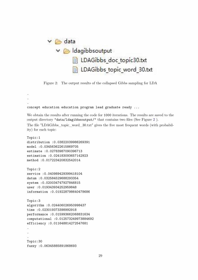
Figure 2: The output results of the collapsed Gibbs sampling for LDA
.
.
.concept education education program lead graduate ready ...
We obtain the results after running the code for 1000 iterations. The results are saved to theoutput directory "data/ldagibbsoutput/" that contains two files (See Figure 2 ).The file "LDAGibbs_topic_word_30.txt" gives the five most frequent words (with probabil-ity) for each topic:
Topic:1distribution :0.03822039986269391model :0.034563622615869705estimate :0.02783987090396713estimation :0.024183093657142923method :0.017223420832542014
Topic:2service :0.040989429399418104datum :0.032584529688293354system :0.020034747927846815user :0.019343934252959848information :0.019228798640478686
Topic:3algorithm :0.024406026950998437time :0.023019373398992918performance :0.015993662068831634computational :0.012573249973884692efficiency :0.011648814272547681...Topic:30fuzzy :0.06345885891868693
29

Figure 3: The output results of the CVB for LDA
method :0.029147466429561415set :0.023490390965404524decision :0.022014632148667942criterion :0.020907813036115507
The file "LDAGibbs_doc_topic30.txt" represents the topic distribution for each document:
Topic1 Topic2 Topic3 ... Topic300.0593 0.129 0.00116 ... 0.001160.00161 0.00161 0.291 ... 0.0177...0.002 0.142 0.0220 ... 0.00125
TopicModel4J also provides a constructor method CVBLDA() for the CVB inference:
public CVBLDA(String inputFile, String inputFileCode, int topicNumber,double inputAlpha, double inputBeta, int inputIterations,
int inTopWords,String outputFileDir)
The meaning of parameters (i.e., inputFile, inputFileCode, etc.) in CVBLDA() is the sameas that in GibbsSamplingLDA(). The following code is to call the CVB inference for LDA:
CVBLDA cvblda = new CVBLDA("data/rawdataProcessAbstracts", "gbk", 30, 0.1,0.01, 1000, 5, "data/ldacvboutput/");
cvblda.CVBInference();
We will obtain the results after 1000 iterations. The results are saved to the output directory"data/ldacvboutput/" that contains two files (See Figure 3 ). Contents for the two files aresimilar to the output results of the collapsed Gibbs sampling for LDA.
Application of Sentence-LDASentence-LDA has been widely used in mining topics from online reviews (Jo and Oh 2011;Büschken and Allenby 2016). Therefore, we select Amazon review data to perform the exper-iment. We first split each review sentence by ".", "!" and "?", and then do the pre-processing
30

for each sentence mentioned in Section 3.2. Finally, the data contains 17,216 reviews. Wegive the input file format of Sentence-LDA as follows:
love lotion--light clean smellsmell wonderful--feel great hand armgood shoe...love comfy shoe--fit glove
where the separator between two sentence in each review is "- -".TopicModel4J offers a constructor method SentenceLDA():
public SentenceLDA(String inputFile, String inputFileCode, int topicNumber,double inputAlpha, double inputBeta, int inputIterations,
int inTopWords, String outputFileDir)
The parameters (e.g., inputFile and inputFileCode) of this constructor method SentenceLDA()is the same as that of the constructor method GibbsSamplingLDA().The following code shows an example that extract topics from Amazon review data.
SentenceLDA sentenceLda = new SentenceLDA("data/amR_process", "gbk", 10, 0.1,0.01, 1000, 5, "data/senLDAoutput/");
sentenceLda.MCMCSampling();
The output files (i.e., "SentenceLDA_topic_word10.txt" and "SentenceLDA_doc_topic_10.txt")are saved to the output directory "data/senLDAoutput/". "SentenceLDA_topic_word10.txt"includes top 5 words and associated probabilities for each topic:
Topic:1game :0.01275375756428569vista :0.010205957681264213xp :0.009926947895803648windows :0.00936158596210724user :0.008854962930613056
Topic:2gift :0.012733120175753194card :0.009475213711876724love :0.00825349878792305product :0.007371149120623172great :0.007099656915300133
Topic:3shoe :0.018754967742061632comfortable :0.015284269721141634
31

wear :0.014974676939932808foot :0.014909499512309897size :0.013312652535548582...Topic:10version :0.009524044352755055program :0.008121748279908579windows :0.007373857041057125run :0.0068012528113114805computer :0.006754509608883265
"SentenceLDA_doc_topic_10.txt" contains the topic distribution for each review, as shownbelow:
Topic1 Topic2 Topic3 ... Topic100.05 0.05 0.55 ... 0.050.05 0.55 0.05 ... 0.05...0.70 0.033 0.033 ... 0.033
Application of HDPIn TopicModel4J, the constructor method HDP() is given as follows:
public HDP(String inputFile, String inputFileCode, int initTopicNumber,double inputAlpha, double inputBeta, double inputGamma,
int inputIterations, int inTopWords, String outputFileDir)
where inputFile denotes the input data that its format is the same as that of GibbsSamplingLDA().The initTopicNumber is the initial topic number. The inputAlpha, inputBeta and inputGammaare the input parameters α0, β and γ of HDP algorithm (See Algorithm 4).In this case, we also use the citation data to illustrate the application of HDP(). The followingcode is to call the HDP algorithm for this data:
HDP hdp = new HDP("data/rawdataProcessAbstracts", "gbk", 3, 0.1, 0.01,0.1, 1000, 5, "data/hdpoutput/");
hdp.MCMCSampling();
We get outputs after running the code for 1000 iterations. In this experiment, we finallyachieve the number of topics withK = 21. The output directory "data/hdpoutput/" includestwo files ("HDP_topic_word_21.txt" and "HDP_doc_topic21.txt"). The contents of thesetwo files are similar to the results of LDA.
Application of DMMThe constructor method DMM() is given as follows:
32
public DMM(String inputFile, String inputFileCode, int clusterNumber,double inputAlpha, double inputBeta, int inputIterations,
int inTopWords,String outputFileDir)
The format of the inputFile is the same as that of GibbsSamplingLDA(). In the following,we perform the experiment using the Amazon review data. The code is given by:
DMM dmm = new DMM("data/amReviews", "gbk", 20, 0.1,0.01, 1000, 5, "data/dmmoutput/");
dmm.MCMCSampling();
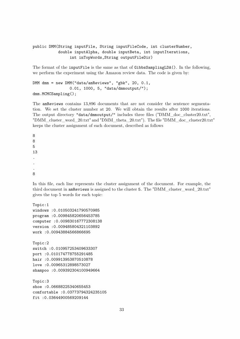
The amReviews contains 13,896 documents that are not consider the sentence segmenta-tion. We set the cluster number at 20. We will obtain the results after 1000 iterations.The output directory "data/dmmoutput/" includes three files ("DMM_doc_cluster20.txt","DMM_cluster_word_20.txt" and "DMM_theta_20.txt"). The file "DMM_doc_cluster20.txt"keeps the cluster assignment of each document, described as follows
88513...8
In this file, each line represents the cluster assignment of the document. For example, thethird document in amReviews is assigned to the cluster 5. The "DMM_cluster_word_20.txt"gives the top 5 words for each topic:
Topic:1windows :0.010503241790570985program :0.009845820656453785computer :0.009830167772308138version :0.009485804321103892work :0.00943884566866695
Topic:2switch :0.010957253409633307port :0.010174778755291485hair :0.009913953870510878love :0.00965312898573027shampoo :0.009392304100949664
Topic:3shoe :0.06688225340655453comfortable :0.03773794324235105fit :0.03644900569209144
33
size :0.03387113059157221great :0.029359849165663563...Topic:20gift :0.06384594555383939card :0.05195676528401261love :0.034568184448847454great :0.031059043135726775product :0.022574253692061848
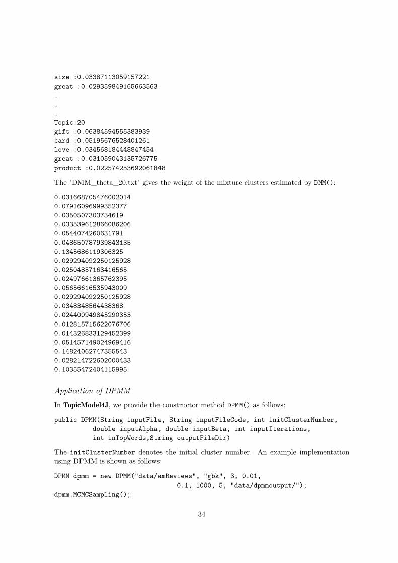
The "DMM_theta_20.txt" gives the weight of the mixture clusters estimated by DMM():
0.0316687054760020140.079160969993523770.03505073037346190.0335396128660862060.05440742606317910.0486507879398431350.13456861193063250.0292940922501259280.025048571634165650.024976613657623950.056566165359430090.0292940922501259280.03483485644383680.0244009498452903530.0128157156220767060.0143268331294523990.0514571490249694160.148240627473555430.0282147226020004330.10355472404115995
Application of DPMMIn TopicModel4J, we provide the constructor method DPMM() as follows:
public DPMM(String inputFile, String inputFileCode, int initClusterNumber,double inputAlpha, double inputBeta, int inputIterations,int inTopWords,String outputFileDir)
The initClusterNumber denotes the initial cluster number. An example implementationusing DPMM is shown as follows:
DPMM dpmm = new DPMM("data/amReviews", "gbk", 3, 0.01,0.1, 1000, 5, "data/dpmmoutput/");
dpmm.MCMCSampling();
34
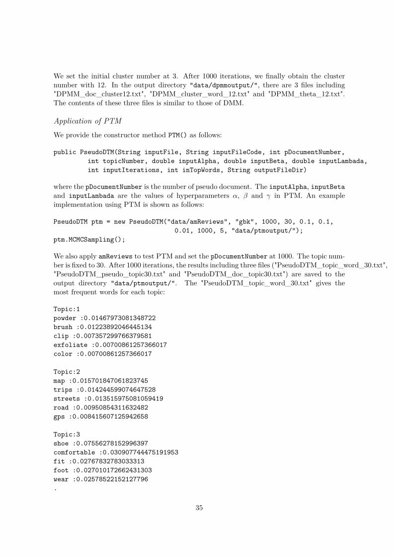
We set the initial cluster number at 3. After 1000 iterations, we finally obtain the clusternumber with 12. In the output directory "data/dpmmoutput/", there are 3 files including"DPMM_doc_cluster12.txt", "DPMM_cluster_word_12.txt" and "DPMM_theta_12.txt".The contents of these three files is similar to those of DMM.
Application of PTM
We provide the constructor method PTM() as follows:
public PseudoDTM(String inputFile, String inputFileCode, int pDocumentNumber,int topicNumber, double inputAlpha, double inputBeta, double inputLambada,int inputIterations, int inTopWords, String outputFileDir)
where the pDocumentNumber is the number of pseudo document. The inputAlpha, inputBetaand inputLambada are the values of hyperparameters α, β and γ in PTM. An exampleimplementation using PTM is shown as follows:
PseudoDTM ptm = new PseudoDTM("data/amReviews", "gbk", 1000, 30, 0.1, 0.1,0.01, 1000, 5, "data/ptmoutput/");
ptm.MCMCSampling();
We also apply amReviews to test PTM and set the pDocumentNumber at 1000. The topic num-ber is fixed to 30. After 1000 iterations, the results including three files ("PseudoDTM_topic_word_30.txt","PseudoDTM_pseudo_topic30.txt" and "PseudoDTM_doc_topic30.txt") are saved to theoutput directory "data/ptmoutput/". The "PseudoDTM_topic_word_30.txt" gives themost frequent words for each topic:
Topic:1powder :0.01467973081348722brush :0.01223892046445134clip :0.007357299766379581exfoliate :0.00700861257366017color :0.00700861257366017
Topic:2map :0.015701847061823745trips :0.014244599074647528streets :0.013515975081059419road :0.00950854311632482gps :0.008415607125942658
Topic:3shoe :0.07556278152996397comfortable :0.030907744475191953fit :0.02767832783033313foot :0.027010172662431303wear :0.02578522152127796.
35
.
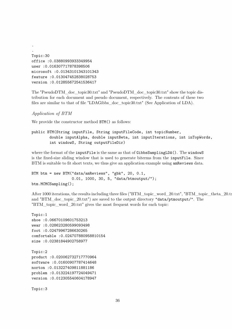
.Topic:30office :0.03880993933349954user :0.016307717878398506microsoft :0.01343101343101343feature :0.013047452838028753version :0.012855672541536417
The "PseudoDTM_doc_topic30.txt" and "PseudoDTM_doc_topic30.txt" show the topic dis-tribution for each document and pseudo document, respectively. The contents of these twofiles are similar to that of file "LDAGibbs_doc_topic30.txt" (See Application of LDA).
Application of BTM
We provide the constructor method BTM() as follows:
public BTM(String inputFile, String inputFileCode, int topicNumber,double inputAlpha, double inputBeta, int inputIterations, int inTopWords,int windowS, String outputFileDir)
where the format of the inputFile is the same as that of GibbsSamplingLDA(). The windowSis the fixed-size sliding window that is used to generate biterms from the inputFile. SinceBTM is suitable to fit short texts, we thus give an application example using amReviews data.
BTM btm = new BTM("data/amReviews", "gbk", 20, 0.1,0.01, 1000, 30, 5, "data/btmoutput/");
btm.MCMCSampling();
After 1000 iterations, the results including three files ("BTM_topic_word_20.txt", "BTM_topic_theta_20.txt"and "BTM_doc_topic_20.txt") are saved to the output directory "data/ptmoutput/". The"BTM_topic_word_20.txt" gives the most frequent words for each topic:
Topic:1shoe :0.06670109601753213wear :0.028623280599093498foot :0.02479967286630265comfortable :0.024707880958810154size :0.02381844902758977
Topic:2product :0.020062732717770964software :0.01600907787414648norton :0.013227409811881186problem :0.013224197724049471version :0.012305540604178947
Topic:3
36

soap :0.04160400014712544scent :0.030190151053877717smell :0.02769318031390717skin :0.023470362150721687bar :0.017099414748002716...Topic:20file :0.019151633443044193drive :0.018554723870893dvd :0.013367495617128413hard :0.01272855015961446video :0.011702874556763115
The "BTM_topic_theta_20.txt" gives the result of the global topic distribution θ.
0.103038970022056050.10153550500502460.07470348328830770.039445140493063440.053271276248645970.0286344178640878070.068050781097059630.0211392793286611060.0261227699254792940.037916226198399960.043573796379677120.0307382248150033270.0239915560601908040.0173421165968442870.034568014825835580.0508562050559231630.067742127037573580.081831238662020550.0567310729154431450.038767798180702924
The "BTM_doc_topic_20.txt" presents the topic proportion for each document.
Topic1 Topic2 Topic3 ... Topic204.572E-4 1.275E-4 0.281 ... 0.007330.0390 0.00469 1.713E-4 ... 1.890E-4...0.139 6.181E-4 3.262E-4 ... 2.697E-5
37

Application of ATM
For ATM, we give an application example using citation data. From the citation data, wefirst extract the author list and abstracts for each paper. For the abstracts, we then use thepre-processing method for the data cleaning. Finally, the input data for ATM contains 1,270documents and its format is described as follows:
Christopher Kruegel, Engin Kirda, ... number application download ...Armando Barreto, Malek Adjouadi paper present statistical result ...Carlos T. Calafate, Juan-Carlos Cano, ... multi-path route technique ......Min Zhang, Shaoping Ma, ... understand kind web page ...
where any two authors in the author list of each paper are separated by a comma (,). Theauthor list and abstracts are separated by Tab spaces (using "\t" to create in Java).We provide the constructor method AuthorTM() as follows:
public AuthorTM(String inputFile, String inputFileCode, String separator,int topicNumber, double inputAlpha, double inputBeta, int inputIterations,int inTopWords, String outputFileDir)
where separator is the separator character of any two authors in the author list. An exampleimplementation using ATM is shown as follows:
AuthorTM atm = new AuthorTM("data/citationAu_process", "gbk", ",", 30, 0.1,0.01, 1000, 5, "data/authorTMoutput/");
atm.MCMCSampling();
Based on this implementation, we finally obtain the results including three files ("authorTM_topic_word30.txt","authorTM_author_topic_30.txt" and "authorTM_topic_author_30.txt") that are saved tothe output directory "data/authorTMoutput/". The "authorTM_topic_word30.txt" presentsthe top 5 words for each topic:
Topic:1graph :0.07544521097384886rule :0.04775083465120365network :0.041638972290344016component :0.03686407982092243edge :0.03361715294171575
Topic: 2image :0.13050785410010649generate :0.05111107941579187multimedia :0.039938479385364364training :0.03304474745169633filter :0.022823006998326487
38
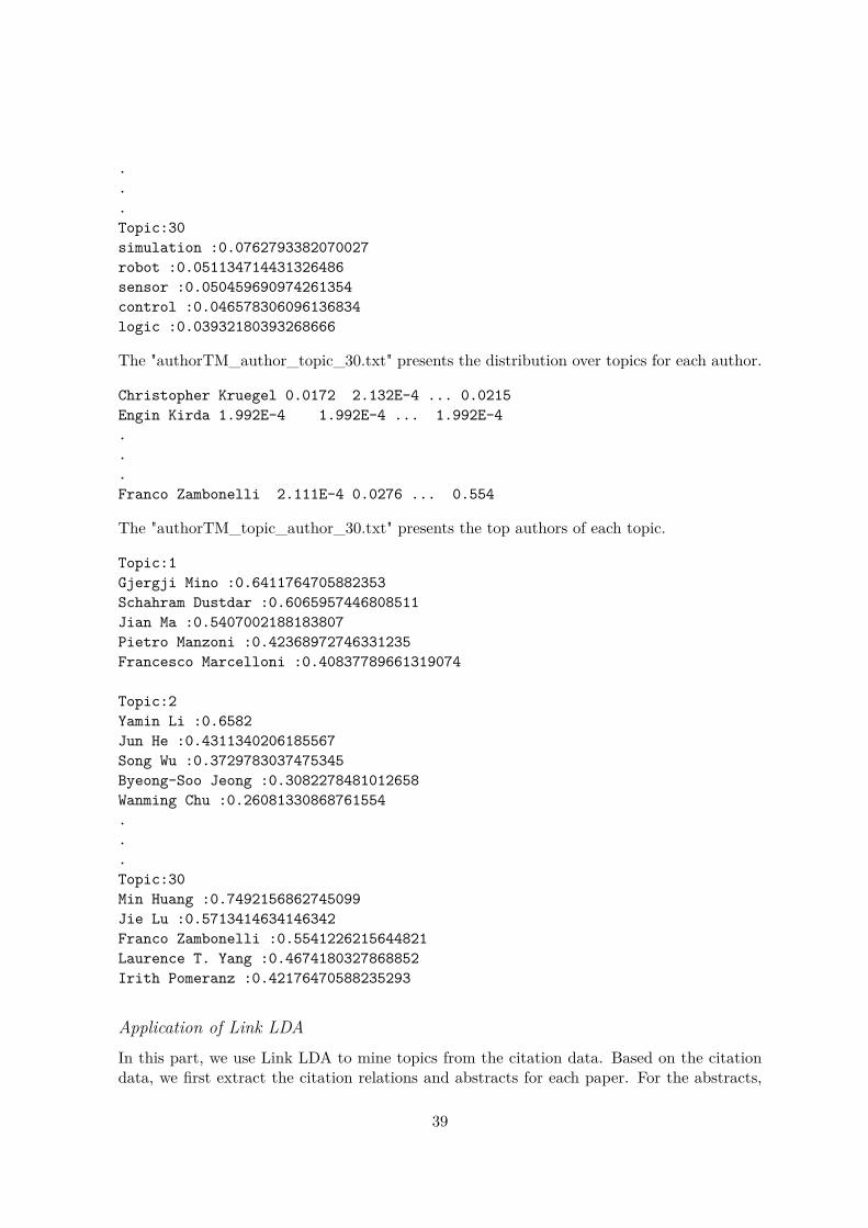
.
.
.Topic:30simulation :0.0762793382070027robot :0.051134714431326486sensor :0.050459690974261354control :0.046578306096136834logic :0.03932180393268666
The "authorTM_author_topic_30.txt" presents the distribution over topics for each author.
Christopher Kruegel 0.0172 2.132E-4 ... 0.0215Engin Kirda 1.992E-4 1.992E-4 ... 1.992E-4...Franco Zambonelli 2.111E-4 0.0276 ... 0.554
The "authorTM_topic_author_30.txt" presents the top authors of each topic.
Topic:1Gjergji Mino :0.6411764705882353Schahram Dustdar :0.6065957446808511Jian Ma :0.5407002188183807Pietro Manzoni :0.42368972746331235Francesco Marcelloni :0.40837789661319074
Topic:2Yamin Li :0.6582Jun He :0.4311340206185567Song Wu :0.3729783037475345Byeong-Soo Jeong :0.3082278481012658Wanming Chu :0.26081330868761554...Topic:30Min Huang :0.7492156862745099Jie Lu :0.5713414634146342Franco Zambonelli :0.5541226215644821Laurence T. Yang :0.4674180327868852Irith Pomeranz :0.42176470588235293
Application of Link LDAIn this part, we use Link LDA to mine topics from the citation data. Based on the citationdata, we first extract the citation relations and abstracts for each paper. For the abstracts,
39

we also use the pre-processing method for the data cleaning. Finally, the input data for LinkLDA contains 18,299 documents and its format is described as follows:
457720--578743--6436976-- ... paper present indoor navigation range ...273266--1065537--11205936-- ... globalisation education topic ...210775--264701--272246-- ... professional software development team base ......
where any two citation indexes cited by each paper are separated by "- -". The citationindexes and abstracts are separated by Tab spaces. In TopicModel4J, the constructor methodLinkLDA() is given as follows:
public LinkLDA(String inputFile, String inputFileCode, String separator,int topicNumber, double inputAlpha, double inputBeta,double inputGamma,int inputIterations, int inTopWords, String outputFileDir)
where separator is the separator character of any two citation indexes. The topicNumber,inputAlpha, inputBeta, inputGamma and inputIterations are the input parameters α, β,γ, and Niter of Link LDA (See Algorithm 10). We give an example to show how to use LinkLDA in our package.
LinkLDA linklda = new LinkLDA("data/citationLink_process", "gbk", "--", 50, 0.1,0.01,0.01, 1000, 5, "data/linkldaoutput/");
linklda.MCMCSampling();
where we set the topic number at 50. According to this code, we will obtain the results in-cluding three files ("LinkLDA_topic_word_50.txt", "LinkLDA_topic_link_50.txt" and "Lin-kLDA_doc_topic_50.txt") that are saved to the output directory "data/linkldaoutput/".The "LinkLDA_topic_word_50.txt" gives the the most frequent words for each topic learnedby Link LDA:
Topic:1model :0.04919313426495349distribution :0.031032042220064535estimate :0.021740932811592357parameter :0.019003608793232284probability :0.018661443290937274
Topic:2program :0.0361938918889249language :0.023070572530579984analysis :0.015965590712367767code :0.01518543584605427tool :0.014015203546584023Topic:3
40
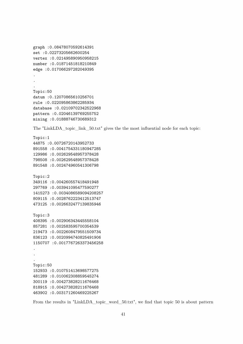
graph :0.08478070592614391set :0.02273205662600254vertex :0.021495890950958215number :0.01871451818210849edge :0.017066297282049395...Topic:50datum :0.12070865610256701rule :0.022095863862285934database :0.02109702342522968pattern :0.02046139769255752mining :0.01888746730689312
The "LinkLDA_topic_link_50.txt" gives the the most influential node for each topic:
Topic:144875 :0.00726720143952733891558 :0.0041754331180947285129986 :0.002629548957378428798508 :0.002629548957378428891548 :0.002474960541306798
Topic:2349116 :0.004260557418491948297769 :0.0039410954775902771415273 :0.0034086589094208257809115 :0.0028762223412513747473125 :0.0026632477139835946
Topic:3408395 :0.002906343445558104857281 :0.002583595700354539219473 :0.0022608479551509734836123 :0.00209947408254919061150707 :0.0017767263373456258...Topic:50152933 :0.010751413698577275481289 :0.010062308859545274300119 :0.004273828211676468818915 :0.004273828211676468463902 :0.003171260469225267
From the results in "LinkLDA_topic_word_50.txt", we find that topic 50 is about pattern
41
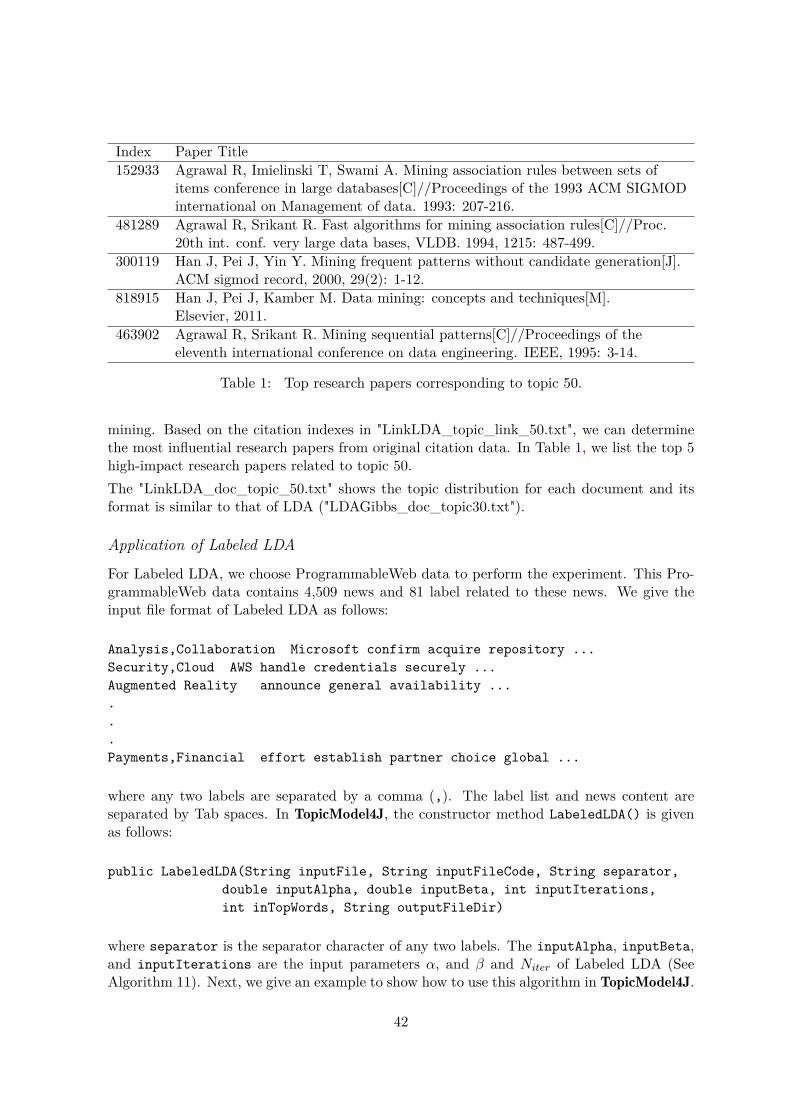
Index Paper Title152933 Agrawal R, Imielinski T, Swami A. Mining association rules between sets of
items conference in large databases[C]//Proceedings of the 1993 ACM SIGMODinternational on Management of data. 1993: 207-216.
481289 Agrawal R, Srikant R. Fast algorithms for mining association rules[C]//Proc.20th int. conf. very large data bases, VLDB. 1994, 1215: 487-499.
300119 Han J, Pei J, Yin Y. Mining frequent patterns without candidate generation[J].ACM sigmod record, 2000, 29(2): 1-12.
818915 Han J, Pei J, Kamber M. Data mining: concepts and techniques[M].Elsevier, 2011.
463902 Agrawal R, Srikant R. Mining sequential patterns[C]//Proceedings of theeleventh international conference on data engineering. IEEE, 1995: 3-14.
Table 1: Top research papers corresponding to topic 50.
mining. Based on the citation indexes in "LinkLDA_topic_link_50.txt", we can determinethe most influential research papers from original citation data. In Table 1, we list the top 5high-impact research papers related to topic 50.The "LinkLDA_doc_topic_50.txt" shows the topic distribution for each document and itsformat is similar to that of LDA ("LDAGibbs_doc_topic30.txt").
Application of Labeled LDA
For Labeled LDA, we choose ProgrammableWeb data to perform the experiment. This Pro-grammableWeb data contains 4,509 news and 81 label related to these news. We give theinput file format of Labeled LDA as follows:
Analysis,Collaboration Microsoft confirm acquire repository ...Security,Cloud AWS handle credentials securely ...Augmented Reality announce general availability ......Payments,Financial effort establish partner choice global ...
where any two labels are separated by a comma (,). The label list and news content areseparated by Tab spaces. In TopicModel4J, the constructor method LabeledLDA() is givenas follows:
public LabeledLDA(String inputFile, String inputFileCode, String separator,double inputAlpha, double inputBeta, int inputIterations,int inTopWords, String outputFileDir)
where separator is the separator character of any two labels. The inputAlpha, inputBeta,and inputIterations are the input parameters α, and β and Niter of Labeled LDA (SeeAlgorithm 11). Next, we give an example to show how to use this algorithm in TopicModel4J.
42
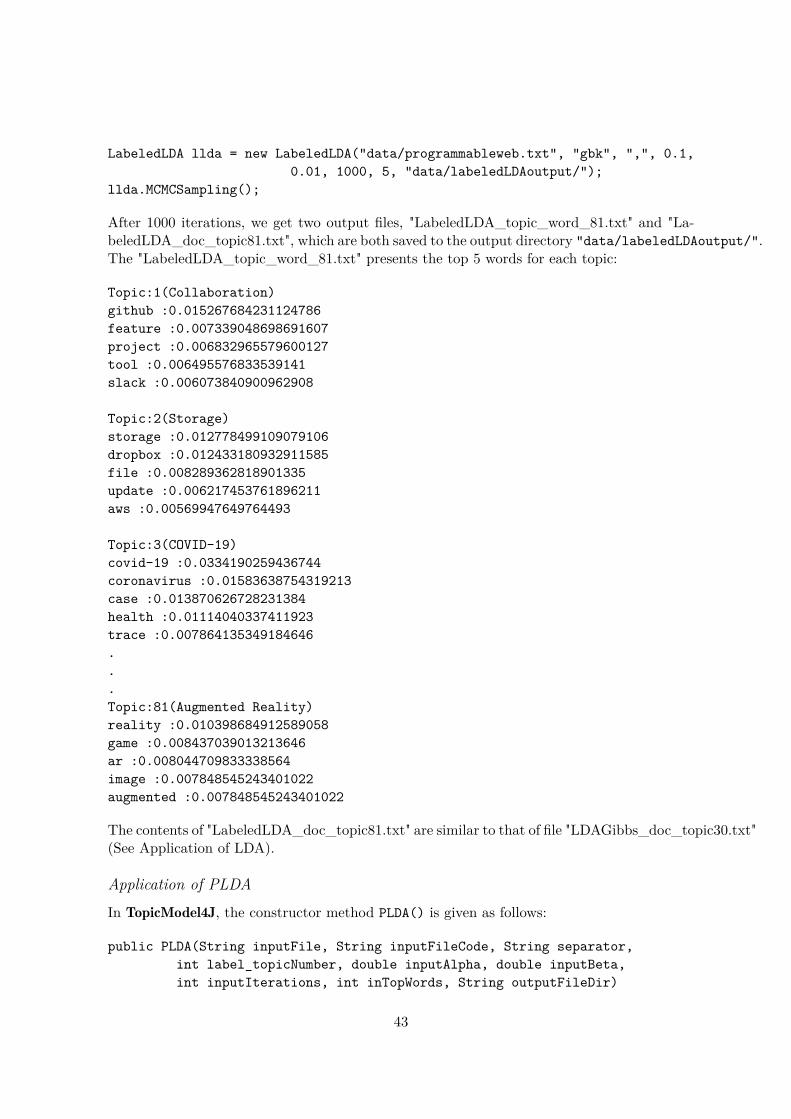
LabeledLDA llda = new LabeledLDA("data/programmableweb.txt", "gbk", ",", 0.1,0.01, 1000, 5, "data/labeledLDAoutput/");
llda.MCMCSampling();
After 1000 iterations, we get two output files, "LabeledLDA_topic_word_81.txt" and "La-beledLDA_doc_topic81.txt", which are both saved to the output directory "data/labeledLDAoutput/".The "LabeledLDA_topic_word_81.txt" presents the top 5 words for each topic:
Topic:1(Collaboration)github :0.015267684231124786feature :0.007339048698691607project :0.006832965579600127tool :0.006495576833539141slack :0.006073840900962908
Topic:2(Storage)storage :0.012778499109079106dropbox :0.012433180932911585file :0.008289362818901335update :0.006217453761896211aws :0.00569947649764493
Topic:3(COVID-19)covid-19 :0.0334190259436744coronavirus :0.01583638754319213case :0.013870626728231384health :0.01114040337411923trace :0.007864135349184646...Topic:81(Augmented Reality)reality :0.010398684912589058game :0.008437039013213646ar :0.008044709833338564image :0.007848545243401022augmented :0.007848545243401022
The contents of "LabeledLDA_doc_topic81.txt" are similar to that of file "LDAGibbs_doc_topic30.txt"(See Application of LDA).
Application of PLDA
In TopicModel4J, the constructor method PLDA() is given as follows:
public PLDA(String inputFile, String inputFileCode, String separator,int label_topicNumber, double inputAlpha, double inputBeta,int inputIterations, int inTopWords, String outputFileDir)
43
where label_topicNumber is the topic number of each label. And the inputAlpha, inputBeta,and inputIterations are other input parameters α, β and Niter of PLDA (See Algorithm12). In the following, we perform the experiment using the ProgrammableWeb data:
PLDA plda = new PLDA("data/programmableweb.txt", "gbk", ",", 2, 0.1, 0.01,1000, 20, "data/pLDAoutput/");
plda.MCMCSampling();
We run the model with 2 global latent background topics and 2 latent topics per label. Theresults including two files ("PLDA_topic_word_82.txt" and "PLDA_doc_topic82.txt") aresaved to the output directory "data/pLDAoutput/". The "PLDA_topic_word_82.txt" showsthe most frequent words for 164 (82*2) topics:
Topic:1 Related label:Collaborationgithub :0.06933694647356305feature :0.025834254744512314slack :0.019036959161848138collaboration :0.01813065308415958project :0.017677500045315302
Topic:2 Related label:Collaborationslack :0.022956225539933324collaboration :0.020540416485480988docusign :0.01933251195825482evernote :0.018728559694641735github :0.0163127506401894...Topic:163 Related label:global labeloffer :0.0064778984884837feature :0.005851266451286184tool :0.0056916149768409564enable :0.005116869668838139system :0.0044982202053628845
Topic:164 Related label:global labelcategory :0.006814344167937558offer :0.006224982169600439tool :0.00542450542559032feature :0.005016936680471616client :0.004967090143298825
The contents of "PLDA_doc_topic82.txt" are similar to that of file "LDAGibbs_doc_topic30.txt"(See Application of LDA).
Application of Dual-Sparse Topic ModelThe Dual-Sparse Topic Model is a method for short documents modeling. In TopicModel4J,
44
we create a constructor method DualSparseLDA() to implement this algorithm:
public DualSparseLDA(String inputFile, String inputFileCode, int topicNumber,double inputS, double inputT, double inputX, double inputY,double inputGamma,double inputGamma_bar,double inputPi,double inputPi_bar,int inputIterations, int inTopWords,String outputFileDir)
where the topicNumber, inputS, inputT, inputX, inputY, inputGamma, inputGamma_bar,inputPi, inputPi_bar and inputIterations are the parameters of Dual-Sparse Topic Model(See Algorithm 13). We give an application example using Amazon review data of "Gift Cards"category. The data about this category contains 1,035 documents.
DualSparseLDA dualSLDA = new DualSparseLDA("data/amReviewsGift", "gbk", 10,1.0, 1.0, 1.0, 1.0, 0.1, 1E-12, 0.1, 1E-12, 1000, 5,"data/dstmoutput/");
dualSLDA.CVBInference();
By this code, we obtain four output files "dualSLDA_topic_word_10.txt", "dualSLDA_doc_topic_10.txt","dualSLDA_sparseRatio_TV10.txt", and "dualSLDA_sparseRatio_DT10.txt". They are savedto the output directory "data/linkldaoutput/". The "dualSLDA_topic_word_10.txt" presentthe top 5 words for each topic:
Topic:1love :0.05572016790679046year :0.04240719351423932daughter :0.031993038967226564gift :0.03189584015804868christmas :0.030028774929986162
Topic:2gift :0.07582170588837109card :0.06280373461792894amazon :0.0408348675386099balance :0.025295763275352393box :0.025185954162112986
Topic:3pizza :0.03393077466446514restaurant :0.02224903253461759food :0.02192767815153133money :0.02086309815322604save :0.020460047932054994...Topic:10gift :0.120324455042531
45
card :0.08482478355137302purchase :0.0643595870624188family :0.023398387843003944idea :0.02277221988826173
The "dualSLDA_doc_topic_10.txt" gives the topic distribution for each document and its for-mat is similar to that of LDA ("LDAGibbs_doc_topic30.txt"). The "dualSLDA_sparseRatio_TV10.txt"shows the sparsity ratio of topic-word distributions and the average sparsity ratio of all topics.
0.95896820171293470.94086336335058310.9445258770011140.95870981711299210.95162854067061640.95463147443490660.96080033444844270.94851436257334350.95626670917938430.9488602951277318average saprse ratio of topic_word:0.9523768975612039
The "dualSLDA_sparseRatio_DT10.txt" shows the sparsity ratio of document-topic distri-butions and the average sparsity ratio of all documents.
0.99999999999190680.56703081086420660.9999999999912975...0.9999999999827707average saprse ratio of doc_topic:0.8804768437274924
3.4. Model Evaluation on Coherence Score
For the probabilistic topic models, there are some metrics to evaluate model fit such asperplexity and coherence score (Lin et al. 2014). Perplexity is calculated by the inverse of thegeometric mean per-word likelihood. The weakness of perplexity is that it disconnects withhuman comprehension of topic quality (Chang, Gerrish, Wang, Boyd-Graber, and Blei 2009).Instead, Mimno, Wallach, Talley, Leenders, and McCallum (2011) propose an automaticmetric, coherence score, to evaluate semantic coherence of the learned topics. Previous studieshave indicated that this metric is correlated well with human judgments of topic quality(Mimno et al. 2011; Newman, Lau, Grieser, and Baldwin 2010). Following Mimno et al.(2011), the coherence score for a topic k is defined as:
C(k;V (k)
)=
N∑n=2
n−1∑l=1
logD(v
(k)n , v
(k)l
)+ 1
D(v
(k)l
) (69)
46

where V (k) =(v
(k)1 , v
(k)2 , · · · , v(k)
N
)represents the top N words in topic k. D
(v
(k)l
)denotes
the number of documents that occur v(k)l . D
(v
(k)n , v
(k)l
)denotes the number of documents in
which words v(k)n and v(k)
l co-occurred.In order to evaluate the overall quality, we use the average coherence score over all the topics:
C = 1K
K∑k=1
C(k;V (k)
)(70)
The average coherence score has been widely used in evaluating the effectiveness of differenttopic models (e.g., LDA and BTM) or determining the number of topics for a specific model(e.g., LDA) (Roberts, Stewart, and Airoldi 2016; Xun, Li, Gao, and Zhang 2017). A highercoherence score indicates better model performance. In TopicModel4J, we provide a Javamethod average_coherence() to implement the metric of coherence score:
public static double average_coherence(int[][] docs, double[][] phi,int topN_word)
where docs denotes the encoding style (two dimensional array) of the input data. phi denotestopic-word distribution learned by a topic model. topN_word denotes the number of top wordsin topics. We give an example to show the use of average_coherence():
GibbsSamplingLDA lda = new GibbsSamplingLDA("data/rawdataProcessAbstracts","gbk", 30, 0.1, 0.01, 500, 5, "data/ldagibbsoutput/");
lda.MCMCSampling();double Ac5 = EstimationUtil.average_coherence(lda.docword, lda.estimatePhi(), 5);double Ac10 = EstimationUtil.average_coherence(lda.docword, lda.estimatePhi(), 10);double Ac20 = EstimationUtil.average_coherence(lda.docword, lda.estimatePhi(), 20);System.out.println("average_coherence_5:\t" + Ac5);System.out.println("average_coherence_10:\t" + Ac10);System.out.println("average_coherence_20:\t" + Ac20);
Running this code in a main method of Java, we can obtain the coherence score for thenumber of topic words N = {5, 10, 20}. The results is presented as follows.
average_coherence_5: -17.377065821012504average_coherence_10: -88.70182574985039average_coherence_20: -392.8932343332532
4. Conclusion and Future WorkTopic models play an prominent role for modeling unstructured text data. This paper in-troduces a Java package, named TopicModel4J, which implements multiple types of topicmodels. For each topic model in TopicModel4J, we provide an easy-to-use interface to esti-mate the latent parameters of the model. For the sake of convenient use for researchers, wegive the detail description on the usage of TopicModel4J package, including data preparationand preprocessing, model estimation and model evaluation. From usage examples, we find
47

that each topic model in TopicModel4J can be easily implemented with a few line of Javacode, and the results can be saved to user specified file directory.Package TopicModel4J is still undergoing active development. For the future work, we wouldlike to add the visualization techniques to this package for visualizing the results, e.g., gen-eration of word clouds using topic-word distributions. In recent years, there are some othervariants of topic models developed by researchers. For example, Blei and Lafferty (2006a)propose a correlated topic model for capturing rich topical correlations. Blei and Lafferty(2006b) propose a dynamic topic model for tracking the time evolution of topics in text data.Wang and Blei (2011) propose a collaborative topic modeling for recommendation tasks. Weplan to add these variants of topic models to TopicModel4J.
AcknowledgmentsThis work is supported by the Major Program of the National Natural Science Foundation ofChina (91846201), the Foundation for Innovative Research Groups of the National NaturalScience Foundation of China (71521001), the National Natural Science Foundation of China(71722010, 91746302, 71872060).
References
Ansari A, Li Y, Zhang JZ (2018). “Probabilistic Topic Model for Hybrid RecommenderSystems: A Stochastic Variational Bayesian Approach.” Marketing Science, 37(6), 987–1008.
Asuncion A, Welling M, Smyth P, Teh YW (2009). “On smoothing and inference for topicmodels.” In Proceedings of the twenty-fifth conference on uncertainty in artificial intelli-gence, pp. 27–34. AUAI Press.
Bi B, Tian Y, Sismanis Y, Balmin A, Cho J (2014). “Scalable topic-specific influence analysison microblogs.” In Proceedings of the 7th ACM international conference on Web search anddata mining, pp. 513–522. ACM.
Blei D, Lafferty J (2006a). “Correlated topic models.” Advances in neural information pro-cessing systems, 18, 147.
Blei DM, Lafferty JD (2006b). “Dynamic topic models.” In Proceedings of the 23rd interna-tional conference on Machine learning, pp. 113–120.
Blei DM, Ng AY, Jordan MI (2003). “Latent dirichlet allocation.” Journal of machine Learningresearch, 3(Jan), 993–1022.
Büschken J, Allenby GM (2016). “Sentence-based text analysis for customer reviews.” Mar-keting Science, 35(6), 953–975.
Chang J, Gerrish S, Wang C, Boyd-Graber JL, Blei DM (2009). “Reading tea leaves: Howhumans interpret topic models.” In Advances in neural information processing systems, pp.288–296.
48
Cheng X, Yan X, Lan Y, Guo J (2014). “Btm: Topic modeling over short texts.” IEEETransactions on Knowledge and Data Engineering, 26(12), 2928–2941.
Erosheva E, Fienberg S, Lafferty J (2004). “Mixed-membership models of scientific publica-tions.” Proceedings of the National Academy of Sciences, 101(suppl 1), 5220–5227.
Gerlach M, Peixoto TP, Altmann EG (2018). “A network approach to topic models.” Scienceadvances, 4(7), eaaq1360.
González-Blas CB, et al. (2019). “cisTopic: cis-regulatory topic modeling on single-cell ATAC-seq data.” Nature methods, 16(5), 397–400.
Griffiths TL, Steyvers M (2004). “Finding scientific topics.” Proceedings of the Nationalacademy of Sciences, 101(suppl 1), 5228–5235.
Hannigan T, et al. (2019). “Topic modeling in management research: Rendering new theoryfrom textual data.” Academy of Management Annals, (ja).
Hornik K, Grün B (2011). “topicmodels: An R package for fitting topic models.” Journal ofStatistical Software, 40(13), 1–30. URL https://cran.r-project.org/web/packages/topicmodels.
Jo Y, Oh AH (2011). “Aspect and sentiment unification model for online review analysis.” InProceedings of the fourth ACM international conference on Web search and data mining,pp. 815–824. ACM.
Li C, et al. (2016). “Topic modeling for short texts with auxiliary word embeddings.” InProceedings of the 39th International ACM SIGIR conference on Research and Developmentin Information Retrieval, pp. 165–174. ACM.
Liang S, et al. (2016). “Dynamic clustering of streaming short documents.” In Proceedings ofthe 22nd ACM SIGKDD international conference on knowledge discovery and data mining,pp. 995–1004. ACM.
Lin T, Tian W, Mei Q, Cheng H (2014). “The dual-sparse topic model: mining focused topicsand focused terms in short text.” In Proceedings of the 23rd international conference onWorld wide web, pp. 539–550. ACM.
Ling G, Lyu MR, King I (2014). “Ratings meet reviews, a combined approach to recommend.”In Proceedings of the 8th ACM Conference on Recommender systems, pp. 105–112. ACM.
Manning CD, Surdeanu M, Bauer J, Finkel JR, Bethard S, McClosky D (2014). “The StanfordCoreNLP natural language processing toolkit.” In Proceedings of 52nd annual meeting ofthe association for computational linguistics: system demonstrations, pp. 55–60.
Mimno D, Wallach H, Talley E, Leenders M, McCallum A (2011). “Optimizing semanticcoherence in topic models.” In Proceedings of the 2011 Conference on Empirical Methodsin Natural Language Processing, pp. 262–272.
Newman D, Lau JH, Grieser K, Baldwin T (2010). “Automatic evaluation of topic coher-ence.” In Human language technologies: The 2010 annual conference of the North Americanchapter of the association for computational linguistics, pp. 100–108.
49
Nigam K, et al. (2000). “Text classification from labeled and unlabeled documents using EM.”Machine learning, 39(2-3), 103–134.
Phan XH, Nguyen CT (2007). “GibbsLDA++: AC/C++ implementation of latent Dirichletallocation (LDA).” Tech. rep. URL http://gibbslda.sourceforge.net/.
Ramage D, Hall D, Nallapati R, Manning CD (2009). “Labeled LDA: A supervised topicmodel for credit attribution in multi-labeled corpora.” In Proceedings of the 2009 Conferenceon Empirical Methods in Natural Language Processing: Volume 1-Volume 1, pp. 248–256.Association for Computational Linguistics.
Ramage D, Manning CD, Dumais S (2011). “Partially labeled topic models for interpretabletext mining.” In Proceedings of the 17th ACM SIGKDD international conference on Knowl-edge discovery and data mining, pp. 457–465. ACM.
Roberts ME, Stewart BM, Airoldi EM (2016). “A model of text for experimentation in thesocial sciences.” Journal of the American Statistical Association, 111(515), 988–1003.
Rosen-Zvi M, Griffiths T, Steyvers M, Smyth P (2004). “The author-topic model for au-thors and documents.” In Proceedings of the 20th conference on Uncertainty in artificialintelligence, pp. 487–494. AUAI Press.
Sethuraman J (1994). “A constructive definition of Dirichlet priors.” Statistica sinica, pp.639–650.
Su S, Wang Y, Zhang Z, Chang C, Zia MA (2018). “Identifying and tracking topic-levelinfluencers in the microblog streams.” Machine Learning, 107(3), 551–578.
Teh YW, Jordan MI, Beal MJ, Blei DM (2005). “Sharing clusters among related groups:Hierarchical Dirichlet processes.” In Advances in neural information processing systems,pp. 1385–1392.
Teh YW, Newman D, Welling M (2007). “A collapsed variational Bayesian inference algorithmfor latent Dirichlet allocation.” In Advances in neural information processing systems, pp.1353–1360.
Wang C, Blei DM (2011). “Collaborative topic modeling for recommending scientific articles.”In Proceedings of the 17th ACM SIGKDD international conference on Knowledge discoveryand data mining, pp. 448–456.
Wang JC, Lee YS, Chin YH, Chen YR, Hsieh WC (2015). “Hierarchical Dirichlet processmixture model for music emotion recognition.” IEEE Transactions on Affective Computing,6(3), 261–271.
Xun G, Li Y, Gao J, Zhang A (2017). “Collaboratively improving topic discovery and wordembeddings by coordinating global and local contexts.” In Proceedings of the 23rd ACMSIGKDD International Conference on Knowledge Discovery and Data Mining, pp. 535–543.
Yan X, Guo J, Lan Y, Cheng X (2013). “A biterm topic model for short texts.” In Proceedingsof the 22nd international conference on World Wide Web, pp. 1445–1456. ACM.
50
Yang T, Jin R, Chi Y, Zhu S (2009). “Combining link and content for community detec-tion: a discriminative approach.” In Proceedings of the 15th ACM SIGKDD internationalconference on Knowledge discovery and data mining, pp. 927–936. ACM.
Yin J, Wang J (2014). “A dirichlet multinomial mixture model-based approach for shorttext clustering.” In Proceedings of the 20th ACM SIGKDD international conference onKnowledge discovery and data mining, pp. 233–242. ACM.
Yin J, Wang J (2016). “A model-based approach for text clustering with outlier detection.”In 2016 IEEE 32nd International Conference on Data Engineering (ICDE), pp. 625–636.IEEE.
Yu G, et al. (2010). “Document clustering via dirichlet process mixture model with featureselection.” In Proceedings of the 16th ACM SIGKDD international conference on Knowledgediscovery and data mining, pp. 763–772. ACM.
Yuan Q, Cong G, Lin CY (2014). “COM: a generative model for group recommendation.”In Proceedings of the 20th ACM SIGKDD international conference on Knowledge discoveryand data mining, pp. 163–172. ACM.
Zhang J, Ghahramani Z, Yang Y (2005). “A probabilistic model for online document clus-tering with application to novelty detection.” In Advances in neural information processingsystems, pp. 1617–1624.
Zuo Y, et al. (2016). “Topic modeling of short texts: A pseudo-document view.” In Proceed-ings of the 22nd ACM SIGKDD international conference on knowledge discovery and datamining, pp. 2105–2114. ACM.
51
Author:Yang QianSchool of ManagementHefei University of TechnologyHefei, Anhui 230009, ChinaE-mail: [email protected]
Yuanchun Jiang (corresponding author)School of ManagementHefei University of TechnologyHefei, Anhui 230009, ChinaE-mail: [email protected]
52